Photometric study of selected cataclysmic variables II ... · PDF file2009: The Journal of...

2009: The Journal of Astronomical Data 15, 1. c© C. Papadaki et al.

Photometric study of selected cataclysmic variables II.

Time-series photometry of nine systems.

C. Papadaki1,2, H.M.J. Boffin3, V. Stanishev4, P. Boumis5,

S. Akras5,6 and C. Sterken1

(1) Vrije Universiteit Brussel, Pleinlaan 2, 1050 Brussels, Belgium

(2) ESO, Casilla 19001, Santiago 19, Chile

(3) ESO, Karl-Schwarzschild-Str. 2, 85748 Garching, Germany

(4) Department of Physics, Stockholm University, 106 91 Stockholm, Sweden

(5) Institute of Astronomy and Astrophysics, National Observatory of Athens,

15236 Athens, Greece

(6) University of Crete, Physics Department, 71003 Heraklion, Crete, Greece

Received June 4, 2008, accepted May 5, 2009

Abstract

We present time-series photometry of nine cataclysmic variables: EI UMa, V844Her, V751 Cyg, V516 Cyg, GZ Cnc, TY Psc, V1315 Aql, ASAS J002511+1217.2,

V1315 Aql and LN UMa. The observations were conducted at various observatories,covering 170 hours and comprising 7,850 data points in total.

For the majority of targets we confirm previously reported periodicities and for someof them we give, for the first time through photometry, their underlying spectro-

scopic orbital period. For those dwarf-nova systems which we observed during bothquiescence and outburst, the increase in brightness was accompanied by a decrease

in the level of flickering. For the eclipsing system V1315 Aql we have covered 9eclipses, and obtained a refined orbital ephemeris. We find that, during this long

baseline of observations, no change in the orbital period of this system has occurred.V1315 Aql also shows eclipses of variable depth.

1

2 C. Papadaki et al.

1 Introduction

Cataclysmic variables (CVs) consist of a low-mass star filling its Roche lobe andtransferring mass to its white-dwarf (WD) companion, a procedure resulting in the

formation of an accretion disc. Due to their unpredictability and diversity leading tovarious types of CVs, these stars have since long been the subject of many studies.

Our aim is to better understand the properties of these systems by detecting

periodicities and by analysing the various physical processes that occur, such asoutbursts, superhumps, eclipses, flickering, etc. Our data will be useful for studying

these CVs in the future, when a system possibly is in a different brightness state. Inthis study we present time-resolved photometric data of nine poorly-studied CVs,

dwarf novae (DN) and nova-likes (NLs) in particular. A deeper study of five moreCVs was published by Papadaki et al. (2006).

2 Observations

During the period 2002–2005 we conducted observations of several targets at fivedifferent observatories: the South African Astronomical Observatory (SAAO), the

Observatorium Hoher List in Germany (OHL), Uccle Observatory (UC) in Belgiumand two observatories in Greece: Kryoneri (KR) and Skinakas (SK). At the SAAOwe used the 1-m telescope equipped with a back-illuminated 1024× 1024, 24-µm

pixel STE4 CCD camera with a field of view (FOV) of 5.′3× 5.

′3. At the OHL,

we used the 1-m Cassegrain-Nasmyth telescope with the 2048×2048, 15-µm pixel

HoLiCam CCD camera with a 2-sided read-out. We used the focal reducer and aneffective FOV of 14.

′1×14.

′1. At UC we used the 0.85-m Schmidt telescope with a

2048×2048, 9-µm pixel Princeton Instruments TE CDD camera with a 30.′1×30.

′1

FOV restricted to an effective FOV of 6.′1 × 6.

′1 on average. At KR, the 1.2-m

Cassegrain telescope with a 512× 512 24-µm pixel CCD camera and a 2.′5× 2.

′5

FOV. Finally, we performed observations with the 1.3-m Ritchey-Chretien telescope

at SK, giving a FOV of 8.′5×8.

′5 and used the 1024x1024 pixel SITe CCD camera.

While most of the observations were obtained without filter, the Johnson-R filterwas occasionally used at SK. Table 1 gives the complete observing log for our 9

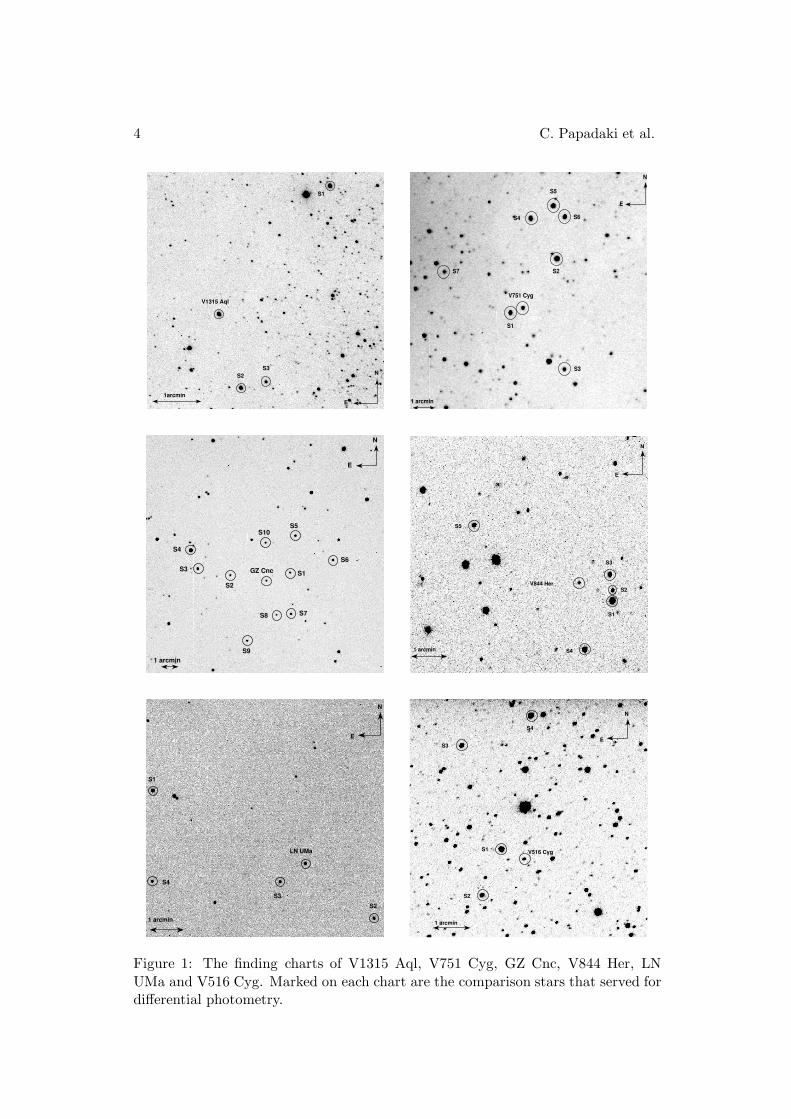
targets. The heliocentric Julian date (HJD) at the beginning of each observingnight, as well as the total duration in hours, are also given. Fig. 1 gives the finding

charts showing the selected comparison stars.

3 Data reduction

The CCD frames were processed for bias removal and flat-field correction. Small

sets of bias frames were taken at regular time intervals during the night, and werethen combined into one median nightly bias frame, which was then subtracted from

all images. In case of significant changes in the CCD temperature, new bias frameswere obtained at that point and neighbouring images were processed with the new

Photometric study of selected cataclysmic variables II. 3

Table 1: Log of observations.UT date Site HJDstart Dur. UT date Site HJDstart Dur.EI UMa GZ Cnc09dec02? OHL 2618.424 2.6 09mar03? OHL 2708.394 2.810dec02 OHL 2619.417 7.7 16mar03? UC 2715.451 0.731jan03? OHL 2671.466 4.7 22mar03 UC 2721.369 0.731jan03? UC 2671.459 5.0 25mar03 UC 2724.430 1.714feb03? UC 2685.461 4.816feb03 UC 2687.315 6.3 TY Psc17feb03 UC 2688.320 8.6 21jul03? SK 2842.526 0.3

22jul03 SK 2843.523 1.2V844 Her 23jul03 SK 2844.491 1.904jul01? UC 2095.423 3.2 10jan05? OHL 3381.255 1.915may02? UC 2410.497 2.016may02 UC 2411.379 5.4 ASAS J0025+1217.212jun02? SK 2438.282 2.0 07oct04? OHL 3286.333 1.714jun02 SK 2440.282 2.5 10oct04 OHL 3289.498 2.015jun02 SK 2441.282 2.5 11oct04 OHL 3290.423 1.8

V751 Cyg V1315 Aql14may04? OHL 3140.446 3.7 14aug03? SAAO 2866.259 2.015may04 OHL 3141.448 0.7 15aug03 SAAO 2867.260 3.516may04 OHL 3142.444 3.5 16aug03 SAAO 2868.275 1.524may04? OHL 3150.529 1.5 17aug03 SAAO 2869.224 4.226may04 OHL 3152.411 4.0 22aug04? KR 3240.287 3.727may04 OHL 3153.411 4.0 31aug04? SK 3249.242 5.428may04 OHL 3154.407 4.3 01sep04 SK 3250.254 5.229may04 OHL 3155.410 2.5 02sep04 SK 3251.267 4.507may05? KR 3498.458 3.308may05 KR 3499.455 3.5 LN UMa09may05 KR 3500.504 2.3 18feb03? UC 2689.452 1.713may05 KR 3504.465 3.5 25feb03 UC 2696.288 9.2

01jun04? SK 3158.330 2.0V516 Cyg 02jun04 SK 3159.375 1.408oct02? UC 2556.319 3.5 06jun04 SK 3163.281 3.009oct02 UC 2557.331 2.819oct02? UC 2567.323 2.023oct02 UC 2571.297 1.405nov02 UC 2584.271 3.2

Notes: HJDstart = HJD−2450000; Dur. is the duration of each observing night in hours; all

observations were obtained without filter, except for the SK measurements of V1315 Aql and LN

UMa, which were made in Johnson-R; ? at the UT date denotes the onset of each observing run.


S3

S2

S1

V1315 Aql

N

E

1arcmin

S7

S6

S5

S4

S3

S2

S1

V751 Cyg

E

N

1 arcmin

E

N

S10

S9

S8 S7

S6

S5

S4

S3

S2

S1GZ Cnc

1 arcmin

S4

S3

S2

S1

LN UMa

E

N

1 arcmin

S5

S4

S3

S2

S1

V844 Her

E

N

1 arcmin

1 arcmin

E

N

S4

S3

S2

S1V516 Cyg

Figure 1: The finding charts of V1315 Aql, V751 Cyg, GZ Cnc, V844 Her, LN

UMa and V516 Cyg. Marked on each chart are the comparison stars that served fordifferential photometry.


S3

E

N

1arcmin

EI UMa

S4

S2

S1

1 arcminE

N

S2

S1

TY Psc

ASAS J002511+1217.12 N

E

1 arcsec

S4

S3

S2

S1

Figure 1: (continued) The finding charts of EI UMa, TY Psc and ASAS

J002511+1217.2. Marked on each chart are the comparison stars that served fordifferential photometry.

combined bias frame. For each night we obtained a median flat-frame. In case ofbad weather during both evening and morning twilight, the flat frame of the closest

observing night was used.

Aperture photometry was performed using the IRAF package apphot. The cir-cular aperture radius used for the computation of the instrumental magnitudes was

equal to 2×FWHM. When the nights were photometric and stable, a mean FWHM

was calculated, resulting in a fixed nightly aperture. In case of unstable sky qual-

ity with strongly variable seeing (as measured by FWHM), the night was dividedinto parts and each part was treated independently by calculating the correspond-

ing aperture. After extracting the instrumental magnitudes of the CV and theselected comparison stars, the following procedure was applied in order to check

the constancy of the comparison stars. The behaviour of the instrumental differ-ential magnitudes of the comparison stars throughout the campaign was checked

and compared to the difference of the instrumental magnitudes between the CV andone comparison star. This was done by plotting the differential magnitudes againsttime. Only when the series of differential magnitudes of a set of comparison stars

did not reveal any night to night trend, and when the standard deviation σ of thecomparison stars’ differential magnitudes was at least 3 times smaller than that of

the CV were the corresponding comparison stars retained for further use. Differ-ential photometry was then applied according to the following procedure. We first

calculated the average instrumental magnitude of each comparison star along withits σ and then determined the weighted average of the instrumental magnitudes of

all comparison stars. The weights for each comparison star were set equal to theinverse of their σ , and the differential magnitudes of each CV were then obtained by


subtracting the weighted average magnitude from the corresponding instrumental

magnitude of the CV.

Given the fact that no filters were used, or if used had to be compared to data

obtained without filters, it was not possible to obtain proper transformations to aphotometric system. However, the following procedure, that yields the most reliablemagnitudes in our case and provides the possibility of comparing to future or past

data, was applied. From the comparison stars we chose those for which Henden &Honeycutt (1995) give V magnitudes. If their catalogue did not contain the required

stars, the respective magnitudes were taken from the online USNO-A2.0 (UnitedStates Naval Observatory) catalogue at ESO (European Southern Observatory) sci-

ence archive facility. For each observing night the catalogued magnitude of eachcomparison star was plotted against the differential magnitude (resulting from the

mean of its differential magnitudes throughout the night) and a linear form wasfitted by least squares. If all nights belonged to the same observing run (defined as

the continuous period of allocated nights at a specific observing site) then a meanequation was calculated and therefore the differential magnitudes of our CV weretransformed to magnitudes that are approximately on the magnitude scale of the

catalogue. When observing runs at different sites were involved, the behaviour ofthe magnitude difference between two comparison stars (common in the FOV of all

observing runs) was checked and the appropriate magnitude shift was applied. Inthis way we were able to compare all light curves obtained at different observatories.

The same reduction technique and light curve generation was applied to all CVsexamined in this study. Table 2 gives the designations of the comparison stars usedfor each target, as seen in Fig. 1, along with their magnitudes and source from the

literature. Whenever any offset occurs it will be stated in the corresponding section.

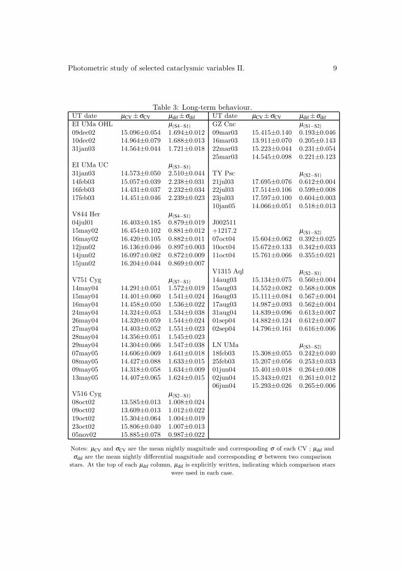
For comparison reasons and in order to have an impression of the range of each

system’s nightly mean-brightness variations, Table 3 gives µCV, which is each sys-tem’s mean nightly magnitude, and µdif, the mean nightly differential magnitudebetween two comparison stars common in the FOV of all observing runs. The com-

parison stars, from which µdif is calculated for each case, are also given.

In addition, when plotting the light curves of all objects in the next sections, an

error bar is shown in the box of each night’s light curve. This serves as an estimationof the error on a single measurement of the magnitude of the CV and is represented

by the standard deviation around the mean of the differential magnitudes betweentwo comparison stars, or else, the scatter in magnitude differences of two comparisonstars. Concerning the choice of the comparison stars, we gave no preference over

stars of smaller scatter for a given magnitude. As long as they fitted the criteriato be chosen (as mentioned earlier in this section), then they were equally treated

for the rest of the procedure. The two stars should ideally be of similar magnitudeas that of the CV. Otherwise, the use of comparison stars that are much fainter

(brighter) would lead to overestimation (underestimation) of the error. However,there are cases where the magnitudes of the available comparison stars differ by

0.5–2mag from that of the CV. In such cases, it was necessary to adopt the followingprocedure, in order to provide a realistic error estimate. Two pairs of comparisons


stars, one pair with magnitudes similar to that of the CV, the other pair with

magnitudes similar to the comparisons we have in the night of interest were lookedfor in another observing night, taking Table 2 into account. Let σ1 and σ2 be the

scatter in magnitude differences for the two pairs, respectively, and σ be the scatterin magnitude differences of the comparisons in the night of interest. Then, the

error on a single measurement is well represented by the quantity σ′= σ1

σ2σ , and is

demonstrated by the error bar in each light curve. Also, it should be pointed out

that due to the change of the FOV between different observing runs of the sameCV, the selected pairs of comparison stars are not necessarily the same between all

observing runs of the same target.

As will be easily noticed from the error bars of the light curves in the upcoming

sections, in most of the cases there are small variations between the nights. Thesevariations are expected due to variations of the weather and therefore atmospheric

conditions. Furthermore, if one CV appears in quiescence during one observingrun and in outburst during another, the error is expected to decrease supposingthere are not any great differences in the atmospheric conditions. However, the

observing site of UC is always subjected to greater errors than the other sites becauseUC is located in a suburb of Brussels and therefore operates under much poorer

atmospheric conditions compared to the rest of the observing sites we used. Inaddition, its low altitude makes it even more vulnerable to the variations of the

lower atmosphere. These are the reasons of the large variance in the errors shownfor some CVs. For V844 Her and LN UMa, the error estimation at UC is 10 and

4 times, respectively, greater than that at SK. For EI UMa, which we observedsimultaneously and under good weather conditions at UC and HL, we found that

the error at UC is 3.5 times greater than that at HL. V516 Cyg, observed only atUC, also shows an increase in the error but this is attributed not only to pooreratmospheric conditions but most predominantly to its decrease in brightness by

2mag.

4 EI UMa

EI UMa (PG 0834+488) was discovered in the Palomar-Green survey (Green et al.,

1982) and was classified as a CV on the basis of its optical spectrum which showedBalmer and high-excitation emission lines. Emission from high-excitation lines ischaracteristic of magnetic CVs. Cook (1985), in the first X-ray study of this target,

found that EI UMa is a hard X-ray source with a low column-density and a ratio ofX-ray to optical density resembling that of DN CVs. This, combined with the facts

that the value of the column density matched that of non-magnetic CVs and, mostimportantly, that there was no X-ray modulation, drew him to the conclusion that

EI UMa better matches a DN. One year later, Thorstensen (1986) performed thefirst radial-velocity study and detected a 6.4-h orbital period (Porb), the spectrum

resembling that of a DN. On the other hand, he was of the opinion that the ratherstrong HeII λ4686 emission, the X-ray characteristics and the system magnitude,


Table 2: Designation of comparison stars.EI UMa GZ CncS1: [HH95] EI UMa-10 V=13.406 S1: U0975 06195484 R=15.7

S2: [HH95] EI UMa-4 V=13.403 S2: U0975 06196461 R=15.5S3: [HH95] EI UMa-23 V=15.922 S3: U0975 06197019 R=14.0

S4: [HH95] EI UMa-32 V=15.168 S4: U0975 06197135 R=13.0S5: U0975 06195399 R=14.7

V844 Her S6: U0975 06194753 R=15.1S1: U1275 08930994 R=13.5 S7: U0975 06195450 R=14.9

S2: U1275 08930976 R=15.7 S8: U0975 06195694 R=15.9S3: U1275 08931020 R=15.4 S9: U0975 06196184 R=15.4

S4: U1275 08931359 R=14.4 S10: U0975 06195886 R=15.3S5: U1275 08932829 R=14.7

TY Psc

V751 Cyg S1: [HH95] TYPsc-24 V=15.240S1: [HH95] V751Cyg-7 V=13.552 S2: [HH95] TYPsc-23 V=15.925

S2: [HH95] V751Cyg-3 V=12.284S3: U1275 14247362 R=14.3 ASAS J002511+1217.2

S4: U1275 14251141 R=12.2 S1: U0975 00086988 R=15.9S5: U1275 14248730 R=12.3 S2: U0975 00086066 R=15.4

S6: U1275 14247527 R=13.7 S3: U0975 00087221 R=16.0S7: U1275 14260111 R=16.3 S4: U0975 00088736 R=16.1

V516 Cyg V1315 AqlS1: U1275 14143883 R=13.9 S1: [HH95] V1315Aql-23 V=14.895

S2: U1275 14144823 R=14.7 S2: [HH95] V1315Aql-38 V=15.992S3: U1275 14145851 R=14.8 S3: U0975 14381457 R=16.3

S4: U1275 14142515 R=13.6LN UMa

S1: [HH95] PG1000+667-13 V=14.307S2: [HH95] PG1000+667-22 V=15.527

S3: [HH95] PG1000+667-21 V=15.859S4: [HH95] PG1000+667-19 V=16.209

Notes: Designations starting with HH95 refer to stars as taken from Henden & Honeycutt (1995).

The rest are adopted from the USNO-A2 catalogue.

implied a possible DQ Her type. One night of photoelectric photometry (Wilsonet al., 1986) showed small amplitude flickering but no larger-amplitude long-term

modulations.

Our dataset consists of observations obtained at OHL (3 nights) and at UC (3

nights). All observations were obtained without filter, and the exposure time variedfrom 45 to 90 sec. Because of the absence of a common couple of comparison stars


Table 3: Long-term behaviour.UT date µCV ±σCV µdif ±σdif UT date µCV ±σCV µdif ±σdif

EI UMa OHL µ(S4−S1) GZ Cnc µ(S1−S2)

09dec02 15.096±0.054 1.694±0.012 09mar03 15.415±0.140 0.193±0.04610dec02 14.964±0.079 1.688±0.013 16mar03 13.911±0.070 0.205±0.14331jan03 14.564±0.044 1.721±0.018 22mar03 15.223±0.044 0.231±0.054

25mar03 14.545±0.098 0.221±0.123EI UMa UC µ(S3−S1)

31jan03 14.573±0.050 2.510±0.044 TY Psc µ(S2−S1)

14feb03 15.057±0.039 2.238±0.031 21jul03 17.695±0.076 0.612±0.00416feb03 14.431±0.037 2.232±0.034 22jul03 17.514±0.106 0.599±0.00817feb03 14.451±0.046 2.239±0.023 23jul03 17.597±0.100 0.604±0.003

10jan05 14.066±0.051 0.518±0.013V844 Her µ(S4−S1)

04jul01 16.403±0.185 0.879±0.019 J00251115may02 16.454±0.102 0.881±0.012 +1217.2 µ(S1−S2)

16may02 16.420±0.105 0.882±0.011 07oct04 15.604±0.062 0.392±0.02512jun02 16.136±0.046 0.897±0.003 10oct04 15.672±0.133 0.342±0.03314jun02 16.097±0.082 0.872±0.009 11oct04 15.761±0.066 0.355±0.02115jun02 16.204±0.044 0.869±0.007

V1315 Aql µ(S2−S1)

V751 Cyg µ(S7−S1) 14aug03 15.134±0.075 0.560±0.00414may04 14.291±0.051 1.572±0.019 15aug03 14.552±0.082 0.568±0.00815may04 14.401±0.060 1.541±0.024 16aug03 15.111±0.084 0.567±0.00416may04 14.458±0.050 1.536±0.022 17aug03 14.987±0.093 0.562±0.00424may04 14.324±0.053 1.534±0.038 31aug04 14.839±0.096 0.613±0.00726may04 14.320±0.059 1.544±0.024 01sep04 14.882±0.124 0.612±0.00727may04 14.403±0.052 1.551±0.023 02sep04 14.796±0.161 0.616±0.00628may04 14.356±0.051 1.545±0.02329may04 14.304±0.066 1.547±0.038 LN UMa µ(S3−S2)

07may05 14.606±0.069 1.641±0.018 18feb03 15.308±0.055 0.242±0.04008may05 14.427±0.088 1.633±0.015 25feb03 15.207±0.056 0.253±0.03309may05 14.318±0.058 1.634±0.009 01jun04 15.401±0.018 0.264±0.00813may05 14.407±0.065 1.624±0.015 02jun04 15.343±0.021 0.261±0.012

06jun04 15.293±0.026 0.265±0.006V516 Cyg µ(S2−S1)

08oct02 13.585±0.013 1.008±0.02409oct02 13.609±0.013 1.012±0.02219oct02 15.304±0.064 1.004±0.01923oct02 15.806±0.040 1.007±0.01305nov02 15.885±0.078 0.987±0.022

Notes: µCV and σCV are the mean nightly magnitude and corresponding σ of each CV ; µdif and

σdif are the mean nightly differential magnitude and corresponding σ between two comparison

stars. At the top of each µdif column, µdif is explicitly written, indicating which comparison stars

were used in each case.


at the two sites, the overlapping observing night of 31 January 2003 was used for

the comparison between the OHL and UC light curves. This was done by equatingthe mean magnitude of our system in the overlapping period of time in the common

observing night. The light curves are shown in Fig. 2. The OHL and UC observingnights in Table 3 are separated since µdif does not correspond to the same couple of

comparison stars.

Figure 2: EI UMa light curves. In the upper left part of each light curve the

error on a single measurement is indicated. The sine curve with P = 3.598 cd−1 is

superimposed on the UC light curves.

In Fig. 2 it is evident that the system’s brightness, if we define two subsets, onefor each observing site, showed an increase by ≈0.6mag in both subsets. Table 3

illustrates the significancy of this increase since the variation of the mean differentialmagnitude between the comparison stars is of a much smaller scale. However, we also

notice that between the two subsets, a great change in the system’s variability occurs.For the subsequent analysis we have therefore treated the two subsets independently.

For EI UMa, as well as the remaining CVs that are presented in this study,frequency analysis was carried out by using the period04 package (Lenz & Breger,2005), based on the Discrete Fourier Transform method. The calculation of the

uncertainties of the corresponding parameters was performed by means of MonteCarlo simulations from the same package. Before performing the frequency analysis,

the trend in the light curves was removed by bringing them around their nightlymean. For the OHL subset we find a frequency of 2.7911±0.0002cd

−1 with a semi-

amplitude of 0.076±0.002mag, along with the second highest peak, its 3.79 cd−1

alias, which corresponds to the frequency of the spectroscopic Porb. This suggests

that even though our data are better fitted by a frequency of 2.7911±0.0002cd−1, the

3.79 cd−1 alias (corresponding to the spectroscopic period) is more likely the right


one. When running frequency analysis on the residuals, a frequency of 9.57 cd−1 or

2.5 h shows up. However, this signal does not occur on a stable time-scale and itsfolding is not promising. If we also consider that the duration of each OHL observing

night is more or less a multiple of 2.5 h, then it is quite possible that 9.57 cd−1 is an

alias frequency caused by the observing strategy.

The UC subset has more to reveal. We have detected a modulation at 3.640±

0.011cd−1 (Fig. 3a) or 6.59h which agrees with the spectroscopic Porb of 6.43h andsemi-amplitude of 0.021±0.002mag. Moreover, it is true that had the periodicitynot been detected spectroscopically, it would have been difficult to trust it. The

sinusoidal representation of the periodicity has been superimposed on the UC lightcurves of Fig. 2. Fig. 3b shows the data folded on the 6.6-h periodicity, while Fig. 3c

shows the folded data after applying 0.005 phase binning.

Figure 3: a) Resulting power spectra of the UC subset with the dominant frequencyindicated b) Data folded on the 6.67-h periodicity c) Folded data, after 0.005 phasebinning.

The standard deviation σ of the measurements in each light curve was also

calculated. Then the average of all σ and its σ as uncertainty, were computed forboth subsets. For the OHL subset it was found equal to 0.059±0.018 and for the

UC subset 0.043±0.006. This implies a decrease in the level of flickering with theincreasing brightness between the two subsets, a behaviour also noticed between

the individual nights. Since the decrease in the level of flickering was followed byan increase on the errors of a single measurement, as indicated in the upper left

corners of the light curves, this makes us more confident that it is indeed the levelof flickering that has changed.

5 V844 Her

V844 Her is a DN discovered by Antipin (1996) on photographic plates. The bestobserved outburst lasted between 12 and 18 days. Since then, various variable

star organisations followed this object. During its first outburst, clear superhumpswere visible (Scovil, 1996; Vanmunster, 1996) and during a superoutburst a period of


0.056±0.001d was found. More precise measurements of the superhump period (Psh)

are given by Kato & Uemura (2000) and Thorstensen et al. (2002) during the 1999and 1997 outbursts, respectively. As Thorstensen et al. (2002) noted, the eruption

timescale, a maximum brightness plateau of more than 10 d with a following rapiddecrease in 1–2 d, as well as the superhumps establish the star’s membership in the

SU UMa class of DN. Quiescent spectra, part of the same study, appeared typicalof those of DN and had double-peaked emission lines. The Porb, measured from the

Hα emission-line velocities, was found to be 0.054643±7·10−6 d.

Figure 4: V844 Her light curves. In the upper left (or right) corner of each lightcurve the error on a single measurement is indicated.

V844 Her was observed during 3 nights at UC and during 3 nights at SK, alldata obtained without filter. The exposure time varied between 120 and 240 sec.

The light curves are shown in Fig. 4. The error bars on the upper left (or right)corners of each light curve indicate the error on a single measurement.

We performed frequency analysis, but no significant periodicity was detected.The σ of the measurements is 0.131±0.047mag for the UC subset and 0.057±

0.022mag for the SK one. However, the error on a single measurement, as indi-cated in the upper left part of each light curve in Fig. 4, is larger in the UC subset

by a similar factor as the difference in σ between the two subsets. Thus we do notthink that the flickering level between the two subsets has significantly changed.

An inspection of the AAVSO long-term light curves1 revealed that we have justmissed a superoutburst in the meantime between the second and third observingrun. The nights of 15 and 16 May 2002 are placed just before the start or at the

1The AAVSO light curve generator tool is at www.aavso.org/data/lcg/. Using as input JD245 2400–2450 and using only the visual-validated data, the superoutburst light curve is generated.Another superoutburst light curve with a more complete coverage is found for JD 245 2150–2181.


rising part of the superoutburst. During the nights of 12–15 June 2002 the system

had returned to quiescence.

6 V751 Cyg

V751 Cyg (EM* LkHα) lies near the “eye” of the Pelican nebula (IC 5070). Itsvariability was discovered by Martynov (1958) and the star was initially believed to

be an R Coronae Borealis star. Later spectra (Herbig, 1958; Herbig & KameswaraRao, 1972) revealed its CV nature. This system had already shown drops up to2.5mag, but it was only after high-speed photometry was obtained, that it was first

suggested to be a NL of the VY Scl subtype (Robinson et al., 1974). This suggestionwas later confirmed by Downes et al. (1995) and Munari et al. (1997), on the basis

of spectra showing Balmer and He emission (or emission cores in some cases), albeitnot of great strength except Hα . V751 Cyg was also identified, during a low state, as

a transient supersoft X-ray source (Greiner et al., 1999). X-ray observations duringthe high state showed that this was not the case. An anti-correlation of X-ray

and optical intensity was also observed. Optical spectra during the same low-staterevealed a very blue continuum and strong emission lines (Balmer, HeI and HeII

λ4686).

The first detailed spectrophotometric study was published by Patterson et al.

(2001). They reported photometric cycles at 3.348 h or f1 = 7.170±0.003cd−1 and

3.9 d or f2 = 0.254± 0.005cd−1 as well as a modulation of the radial velocities at

3.468h. These signals were identified as a negative superhump period P−sh

, the wob-bling period of a tilted accretion disc Pwob and Porb, respectively. Occasionally the

system showed P Cygni absorption profiles in the Balmer and HeI lines, correlatedwith the binary phase.

Our dataset consists of 8 nights of observing at OHL and 4 nights at KR. Allobserving nights were done without filter, and the exposure time varied between 20

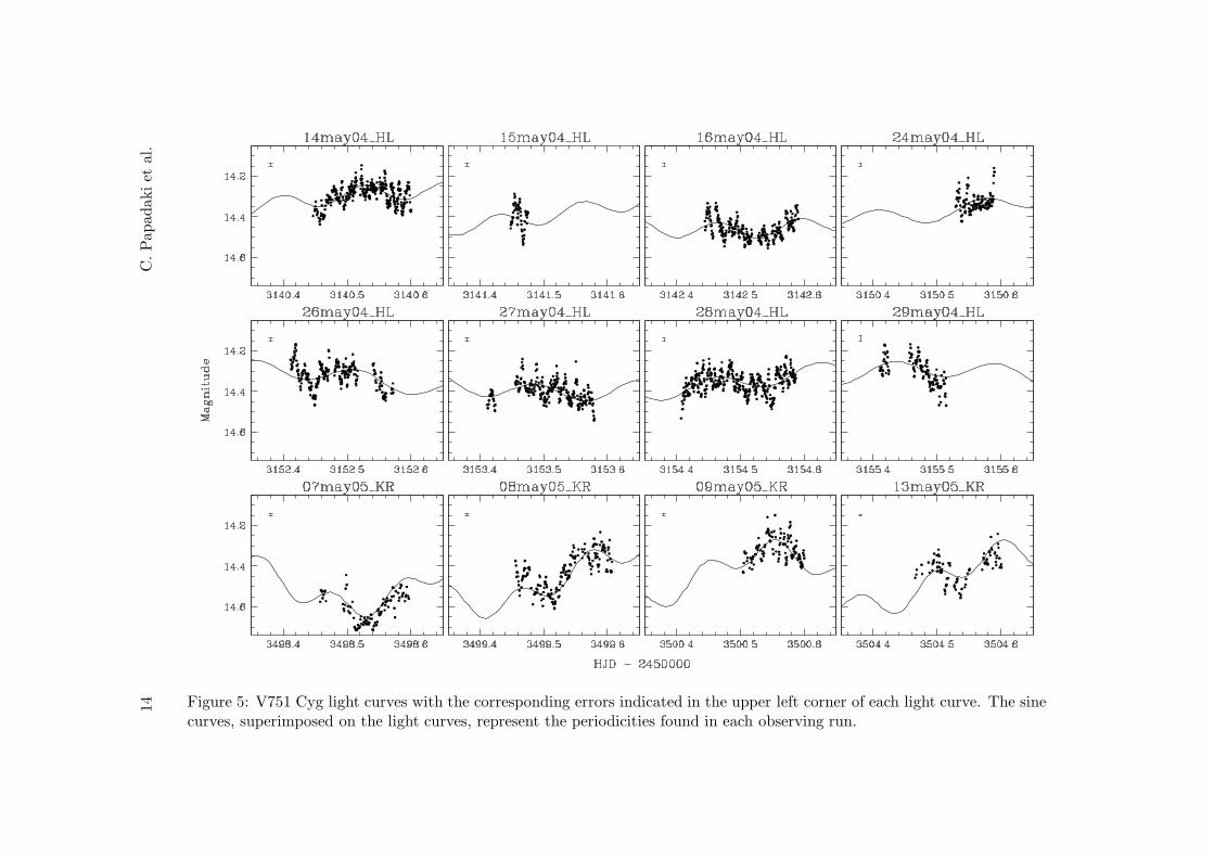
and 80 sec, depending on the telescope and atmospheric conditions. The light curvesare shown in Fig. 5.

The photometric frequencies, found by Patterson et al. (2001), are also detectedin our data, albeit as their aliases or harmonics in some cases. Before applying

frequency analysis, our dataset was divided into 3 subsets, one for each observingrun. In all cases we cannot directly detect the low frequency f2. In the first sub-set we find its 3

rd harmonic, in the second its 1.27 cd−1 alias and in the third its

2.21cd−1 alias. In contrast to Patterson et al. (2001), the number of each subset’s

consecutive observing nights is not larger than 4. This makes the direct detection of

the ≈4-d Pwob more difficult. Performing period analysis on the residuals revealedthe existence of P−

sh. The corresponding frequencies for the first, second and third

subset are 7.739±0.005, 6.171±0.002 and 9.144±0.004cd−1, respectively. The first

signal reflects the combination of frequencies f1 + 2 f2 (or an harmonic of the first

frequency found in the same subset), and the other two aliases of f1. The powerspectra of the original and residual data are shown in the top and bottom row of

14

C.Papadakiet

al.

Figure 5: V751 Cyg light curves with the corresponding errors indicated in the upper left corner of each light curve. The sinecurves, superimposed on the light curves, represent the periodicities found in each observing run.


Fig. 6. Each column from left to right corresponds to the first, second and third

subset, respectively. Both periodicities found in each subset are superimposed onthe lights curves of Fig. 5. The aliases of both periodicities as well as the harmonics

of P−sh

are evident. As seen in Fig. 6a–6c, the aliases are strong, and they dominatethe periodogram in the vicinity of P−

shand bias its estimate. We therefore first fitted

the 4-d period, then subtracted it and finally ran periodogram analysis again. Oncemore the aliases appeared stronger. We also applied the same procedure in the whole

of the OHL observing nights (i.e. subset 1 and 2) but again we could not detect f1

but its 6.17 cd−1 alias. Treating all light curves as a whole, once more reveals the

1.27 cd−1 alias of f2 and the 6.17 cd

−1 alias of P−sh

when period analysis is carried outon the residuals. After subtracting all periodic signals the σ of the measurementswas found to be 0.048±0.007mag.

Figure 6: V751 Cyg power spectra with the dominant frequencies indicated. a, b and

c correspond to the power spectra of the first, second and third subset, respectively.d, e and f are the power spectra of the residuals of the first, second and third subset,

respectively.

The power spectra of CVs show so called “red noise”, thought to originate fromthe flickering through a shot noise-like process. This is demonstrated by the power-

law decrease of the power with the frequency which is represented by a line in log-logscale. In this way, the power-law index γ is used for the characterisation of flickering

activity. According to theoretical studies, γ = 2 corresponds to shots of infinite rise-time and exponential decay, shots of totally random duration and shape. Lower


values correspond to shots with different duration and distribution, that are neither

random nor stable. For more information on “red noise” and γ interpretation, werefer to Papadaki et al. (2006) and references therein. “Red noise” is also present

in our case and therefore the linear part, from 100 cd−1 on, was fitted by a least

squares fit. We found γ = 1.41±0.03 for the OHL observing runs, γ = 1.17±0.03

for the KR observing run and γ = 1.29±0.02 for all runs. However, due to the noisycharacter of the power spectra, small changes in the fitting interval cause changes

in the value of γ up to 0.1, 0.15 and 0.13 for the OHL, KR and all observing runs,respectively. These more realistic γ errors should be adopted instead. It has to be

mentioned that when Patterson et al. (2001) applied the same procedure for theirpower spectra they found γ = 2. In our case the lower γ suggests a different shotdistribution.

7 V516 Cyg

Despite its early discovery as a variable star (Hoffmeister, 1949) V516 Cyg wasonly noticed to be a DN by Meinunger (1966). It was decades later, that the first

optical spectrum was obtained and V516 Cyg was confirmed to be a DN (Bruch &Schimpke, 1992). The spectrum showed a strong blue continuum with Balmer andHe I lines in emission. The Balmer emission lines were superimposed on absorption

troughs, characteristic of DN declining from (or rising to) an outburst. The firstBVRI photometric study during the decline from outburst was conducted by Spogli

et al. (1998), who favoured an outside-in outburst. Spogli et al. (2000) covereda complete outburst cycle. The long-term light curves can be found in the two

aforementioned studies. The light curve of V516 Cyg during the whole outburstcycle pointed to the SS Cyg subclass of CVs.

V516 Cyg was observed at UC during 5 nights. No filter was used and theexposure time varied between 30 and 60 sec. The light curves are shown in Fig. 7.

During the first observing run the system was at the peak of an outburst, confirmedby AAVSO long-term light curves. During the second observing run the system wasreturning to quiescence, having reached it the last night. The magnitude difference

between the two states was ≈2.5mag.

Frequency analysis was applied to the whole dataset, as well as to the two observ-

ing runs independently, but no dominant periodicity was revealed. The system’s de-crease in brightness was followed by an increase in σ , found to be 0.0129±0.0004mag

in outburst. Although still greater, the σ of the measurements during quiescence,in reality, is not much different than that of outburst since the errors on a single

measurement have increased almost proportionally to σ . This implies that there isprobably no change in the level of flickering.


Figure 7: V516 Cyg light curves. In the upper left corner of each light curve theerror on a single measurement is shown.

8 GZ Cnc

GZ Cnc (Tmz V034, RX J0915.8+0900) was discovered by Takamizawa (1998) andidentified as a ROSAT source by Bade et al. (1998). Jiang et al. (2000) obtained

the first optical spectrum which confirmed it as a CV. Some noticeable brightenings(Kato et al., 2001) stimulated interest in monitoring it, and the detection of several

outbursts confirmed it as a DN (Kato et al., 2001, 2002). Photometry during thedecline from outburst (Kato et al., 2001) suggested that GZ Cnc should be a long-period DN, probably of the SS Cyg subtype. This was based on the facts that GZ

Cnc showed no superhumps, had a low outburst amplitude and a slow rising at arate similar to CVs of the SS Cyg subtype. Their dataset consists of 3 nights, the

longest one spanning ≈3.3 h. The long-term light curve of GZ Cnc was studied byKato et al. (2002): GZ Cnc showed anomalous clusterings of outbursts in 2002 –

in contrast to earlier years – and these authors associated this with the behaviourseen in some intermediate polars (IPs). This would result in a period greater than

3h. However, radial velocities of the Hα emission line revealed the system’s Porb

of 2.118±0.007h (Tappert & Bianchini, 2003). The same study also favoured the


IP model due to the strength of the HeII line and the appearance of an absorption

component during the rise to outburst. They summed up that even though therewere strong indications that GZ Cnc could be an IP, these indications could by no

means be conclusive. Both high-speed photometry and time-resolved spectroscopycould clarify its classification.

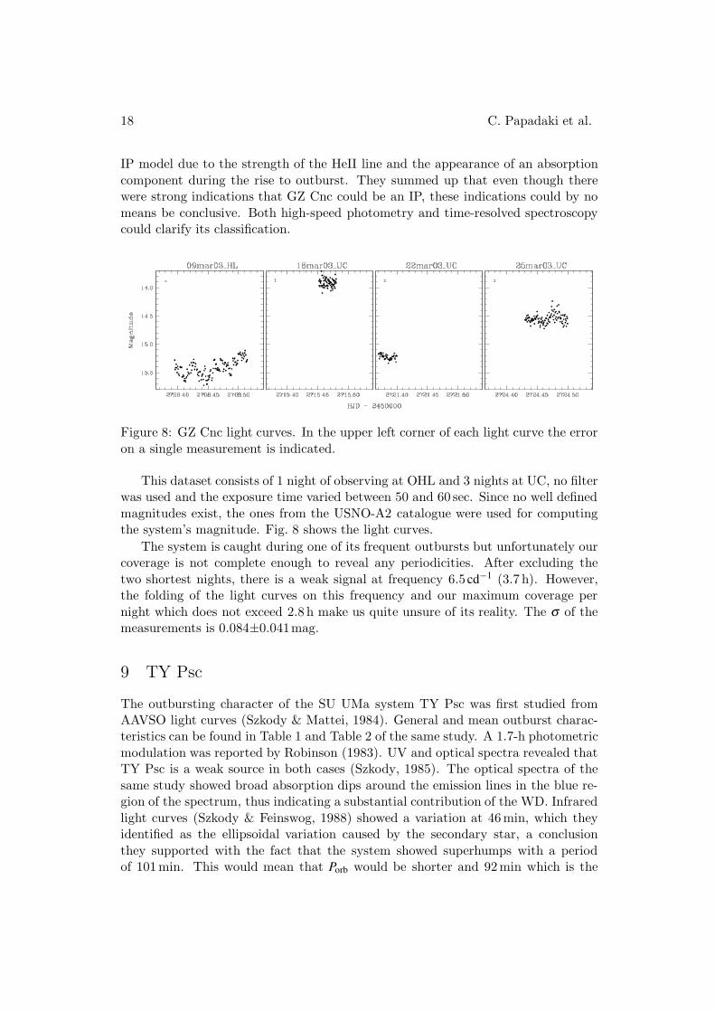
Figure 8: GZ Cnc light curves. In the upper left corner of each light curve the error

on a single measurement is indicated.

This dataset consists of 1 night of observing at OHL and 3 nights at UC, no filterwas used and the exposure time varied between 50 and 60 sec. Since no well defined

magnitudes exist, the ones from the USNO-A2 catalogue were used for computingthe system’s magnitude. Fig. 8 shows the light curves.

The system is caught during one of its frequent outbursts but unfortunately ourcoverage is not complete enough to reveal any periodicities. After excluding the

two shortest nights, there is a weak signal at frequency 6.5 cd−1 (3.7 h). However,

the folding of the light curves on this frequency and our maximum coverage per

night which does not exceed 2.8 h make us quite unsure of its reality. The σ of themeasurements is 0.084±0.041mag.

9 TY Psc

The outbursting character of the SU UMa system TY Psc was first studied fromAAVSO light curves (Szkody & Mattei, 1984). General and mean outburst charac-teristics can be found in Table 1 and Table 2 of the same study. A 1.7-h photometric

modulation was reported by Robinson (1983). UV and optical spectra revealed thatTY Psc is a weak source in both cases (Szkody, 1985). The optical spectra of the

same study showed broad absorption dips around the emission lines in the blue re-gion of the spectrum, thus indicating a substantial contribution of the WD. Infrared

light curves (Szkody & Feinswog, 1988) showed a variation at 46min, which theyidentified as the ellipsoidal variation caused by the secondary star, a conclusion

they supported with the fact that the system showed superhumps with a periodof 101min. This would mean that Porb would be shorter and 92min which is the


double of the ellipsoidal variation would be a good fit. Also their J−H values sup-

ported a large contribution of the secondary star. The same authors gave a roughestimate of the inclination at 55◦. Spectrophotometry by Thorstensen et al. (1996)

confirmed the strong WD contribution as noted before by Szkody (1985), as wellas a Porb of 98.4min, from both radial velocities and photometry. Both the orbital

modulation and double-peaked emission lines pointed to a rather high inclination,while the hot spot was also identified in the light curve. Ciardi et al. (1998) per-

formed time-resolved near-infrared broadband photometry and concluded that thesecondary star contributed less than 20% of the infrared flux, therefore opposing the

idea of the ellipsoidal variation (Szkody & Feinswog, 1988). Their light curve wasquite similar to the optical one (Thorstensen et al., 1996). This resemblance wasinterpreted as a result of the hot spot in the accretion disc dominating the emission

and not as the secondary star contribution, which they found insufficient. Last, thesuperhump period of 101.9min was confirmed through observations during the 2000

superoutburst (Kunjaya et al., 2001).

Figure 9: TY Psc light curves. In the upper left corner of each light curve the

error on a single measurement is indicated. The light curves on top and bottom leftcorrespond to quiescence, while the light curve on bottom right to outburst.


TY Psc was observed at both SK and OHL for 3 and 1 nights, respectively. The

exposure time was 40–120 sec and no filters were used. Fig. 9 shows the light curveduring the SK observing run with TY Psc in quiescence (top row and bottom row

on the left), and during the OHL observing run with TY Psc in outburst (bottomrow on the right).

Frequency analysis was performed during quiescence (SK light curves) and afrequency of 11.60±0.02 cd

−1 with a semi-amplitude of 0.14±0.01mag was found.

This frequency corresponds to 14.63 cd−1, an alias of the orbital frequency, and the

power spectrum reveals the large number of aliases around this frequency, including

the orbital one. Our periodicity of 2.01h is overplotted on the light curves of Fig. 9.For a check we also tried to fold the light curves on Porb, something that gave subtle

differences. Concerning the single night in outburst, we did not use it in the analysis.The corresponding light curve in Fig. 9 also indicates that Porb would not fit. The

system, as confirmed by AAVSO light curves, had just started its decline from theoutburst peak. Such a fast decline (≈3 d for this system) seems to temporarily alterthe morphology of the light curve.

After removing the periodicity from the SK light curves and the trend from

the OHL one, we obtained σ = 0.042± 0.003mag and 0.012± 0.004mag for thequiescence and outburst, respectively. This implies a decrease in the level of flickeringsince the errors of the measurements have not changed significantly.

10 ASAS J002511+1217.2

ASAS J002511+1217.2 (1RXS J002510.8+121725) was discovered by Pojmanski

(2002) and the All-Sky Automated Survey (ASAS). It was also detected by ROSAT(Voges et al., 1999). Upon an alert of a dramatic increase in brightness, astronomers

started following the object for a 2-month period. The long-term light curve, firstpresented by Golovin et al. (2005), revealed that ASAS J002511+1217.2 was an

excellent WZ Sge candidate. The same light curves, accompanied by spectroscopicobservations, were extensively studied by Templeton et al. (2006) who classified itas a new WZ Sge star. WZ Sge stars have infrequent large-amplitude outbursts, or-

bital periods around 2h, show superhumps, and a slow decline from maximum lightto quiescence during which echo outbursts are occasionally formed. Echo outbursts

resemble DN outbursts and appear directly after the main outburst. They are ofabout similar amplitude and recurrence time while after their complete cessation the

system slowly returns to quiescence (Patterson et al., 2002). ASAS J002511+1217.2does not lack any of these characteristics and the results of Templeton et al. (2006)

will now be briefly presented.

The system’s light curve spans three months (mid-September 2004 – mid-December

2004) and during that period the system declined by ≈7mag. The early abrupt de-cline was followed by one echo outburst and the decay time to quiescence lasted

≈90 days. Time-series CCD photometry during the early outburst showed clearsuperhumps at 81.9min shifting around this value as the system faded. During the


quiescent state, just prior to the echo outburst, variations at 81.6min were detected.

During the echo outburst there appeared to be weak variations of the same periodas the original superhumps. A few nights of photometry during the late outburst

(after the echo outburst) showed signals at periods nearly the same as the super-humps, however, it was not as easy to distinguish due to the increased photometric

noise. Time-series spectroscopic observations, well into the object’s decline, yieldeda Porb of 82±5min, albeit not too precise. Narrow and broad components in the

emission-line spectra indicated the presence of multiple emission regions.

ASAS J002511+1217.2 was observed during 3 nights at OHL, right after the 2004

echo outburst. The exposure varied between 15 and 60 sec, and the light curves areshown in Fig. 10.

Our observations lying after the end of the echo outburst show similar results

with Templeton et al. (2006). We find a frequency of 13.42±0.12cd−1 with a semi-

amplitude of 0.08±0.01mag and an alias of the superhump modulation. However,

the folding is not satisfactory. The residual σ of the measurements is 0.070±0.017.

Figure 10: ASAS J002511+1217.2 light curves. In the upper left corner of each light

curve the error on a single measurement is indicated.

11 V1315Aql

V1315 Aql (KPD 1911+1212, SVS 8130) was discovered and suspected as a variablestar by Metik (1961). Later on, based on a spectrophotometric study, Downes et al.(1986) classified this object as an eclipsing CV, with an eclipse depth up to 1.8mag

in V . Porb was found to be 3.35h. Apart from Balmer and HeI emission lines thespectra showed strong high-excitation lines. Even though the HeII λ4686 was totally

eclipsed, the Balmer lines were not. A prominent absorption component was visibleat phase 0.5.

These spectral characteristics, combined with the occurrence of single-peakedemission lines despite the system’s high inclination (Szkody & Piche, 1990), uncom-

mon at that time, provided the impetus for the system’s follow up and the emergenceof a new sub-class of NL CVs, the SW Sex stars. A detailed spectroscopic study


by Dhillon et al. (1991) showed that the spectra of V1315 Aql have: (1) narrow

single-peaked Balmer and HeI lines exhibiting a double-peaked structure near phase0.5 and (2) high-excitation lines, remaining single-peaked throughout the orbit and

being totally eclipsed in contrast to Balmer and HeI lines. They presented the firstDoppler maps which showed a contaminating emission around phase 0.75 and no disc

emission. They connected this to the large phase shifts seen in the radial-velocitymeasurements of all emission lines. Even though the subsequent Doppler maps pre-

sented by Kaitchuck et al. (1994) appeared quite similar, there was disagreementconcerning the origin of the HeII peak emission. Although Dhillon et al. (1991) did

not find it to coincide with the expected location of the WD, Kaitchuck et al. (1994)did. In this way they drew the conclusion that HeII is mostly emitted from a regionvery close to the WD and is therefore a good indicator of the WD orbital motion.

Further spectroscopy (Friend et al., 1988; Smith et al., 1993) showed a strongabsorption feature at the OI triplet λ7773. A detailed study by Smith et al. (1993)

concluded that this feature must arise from some absorbing material that is dis-tributed in a non-axisymmetric manner. This asymmetry seemed to be confined

only to OI. Infrared spectroscopy showed no evidence for the secondary star (Dhillonet al., 2000). For an analytic presentation of a model that could describe the char-

acteristics and peculiarities of V1315 Aql, as well as previous attempts on the samesubject, see Hellier (1996) and references therein. In short, the model combines the

occurrence of both disc overflow and a strong wind, which might result from highmass-transfer rate.

V1315 Aql was observed at SAAO (4 nights), at SK (3 nights) and at KR (1night). At SK observing run the Johnson-R filter was used, while the rest of the

observing runs were done without filter. The exposure time was 40-60 sec. The lightcurves are shown in Fig. 11.

V1315 Aql was observed during two periods, August 2003 and August–September

2004. In total, the system was caught during nine eclipses but, only six of them werefully covered and are therefore used for further analysis. The timings of mid-eclipse,

determined by fitting a Gaussian to the lower half of the eclipses, are given in Table 4.The same table also includes all previously reported minima and their corresponding

cycle number E. The refined ephemeris resulting from all available eclipse timingsis:

Tmid−ecl[HJD] = 2445902.7007 + 0d.139689959E

±0.0001 ±0.000000005

Fig. 12 shows the O −C diagram of all available minima. O represents the

observed times of minima and C the calculated ones according to the ephemeris. Inagreement to all previous studies, no evidence of any kind of curvature or trend is

found in the O−C diagram. This means that in the now even longer baseline of 20years there is no indication of a change in the system’s period.

A look at Fig. 12 shows that there is a large scatter of data points at the first andlast block of data. However, concerning the last block belonging to our observations,


Figure 11: V1315 Aql light curves. In the upper left corner of each light curve the

error on a single measurement is indicated.

the variations we are looking at are of the order of 40–50 sec, i.e. of the size of the

exposure times and therefore they should not be of any significance. Unfortunately,no errors are given on any of the previous studies and so we can not reach any

conclusion about the even larger scatter of the first block.

E

Figure 12: O−C diagram for the timings of mid-eclipse of all available data (seeTable 4).

The application of frequency analysis, after removal of the eclipse data, gives a

frequency of 5.14627±3 ·10−5

cd−1 an alias of the orbital frequency. We also searched

for long-term periodicities, but none was evident. The σ of the measurements is


Table 4: Eclipse timings of V1315 AqlTmid−ecl E Source

(HJD-2445000)

902.84065 1 Downes et al. (1986)906.75180 29 Downes et al. (1986)928.82167 187 Annis (1986)

944.74793 301 Downes et al. (1986)944.88716 302 Downes et al. (1986)

945.72697 308 Annis (1986)945.86459 309 Downes et al. (1986)

971.70748 494 Downes et al. (1986)1295.78815 2814 Annis (1986)

1324.70424 3021 Annis (1986)1344.67928 3164 Annis (1986)

2279.62471 9857 Dhillon et al. (1991)2686.54156 12770 Dhillon et al. (1991)2686.68121 12771 Dhillon et al. (1991)

2788.37501 13499 Dhillon et al. (1991)2790.47069 13514 Dhillon et al. (1991)




2800.38867 13585 Dhillon et al. (1991)2801.36637 13592 Dhillon et al. (1991)4579.6195 26322 Hellier (1996)

7867.36291 49858 This study7869.31812 49872 This study



0.117±0.034mag.

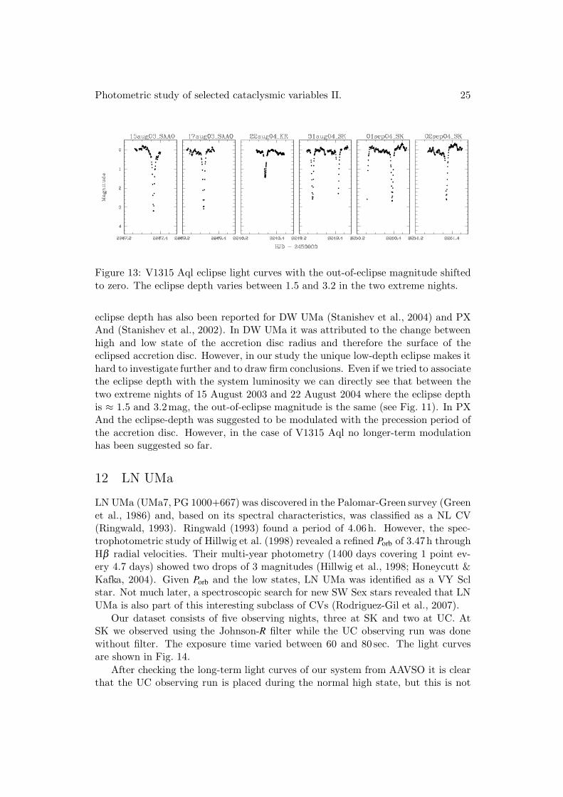
As previously mentioned, V1315 Aql undergoes eclipses of around 1.8mag in

V . In our case the eclipse depth is found around 3.2 and 2.6mag in the 2003(data obtained without filter) and R-band 2004 observing run, respectively. The

only exception is the eclipse depth of the night of 22nd August 2004 (data obtained

without filter), with an eclipse depth that is remarkably smaller at 1.5mag, half or

less than half of the rest of the nights. In Fig. 13 the out-of-eclipse magnitude hasbeen shifted to zero and the variable eclipse depth is readily estimated. Variable


Figure 13: V1315 Aql eclipse light curves with the out-of-eclipse magnitude shifted

to zero. The eclipse depth varies between 1.5 and 3.2 in the two extreme nights.

eclipse depth has also been reported for DW UMa (Stanishev et al., 2004) and PXAnd (Stanishev et al., 2002). In DW UMa it was attributed to the change between

high and low state of the accretion disc radius and therefore the surface of theeclipsed accretion disc. However, in our study the unique low-depth eclipse makes it

hard to investigate further and to draw firm conclusions. Even if we tried to associatethe eclipse depth with the system luminosity we can directly see that between the

two extreme nights of 15 August 2003 and 22 August 2004 where the eclipse depthis ≈ 1.5 and 3.2mag, the out-of-eclipse magnitude is the same (see Fig. 11). In PXAnd the eclipse-depth was suggested to be modulated with the precession period of

the accretion disc. However, in the case of V1315 Aql no longer-term modulationhas been suggested so far.

12 LN UMa

LN UMa (UMa7, PG 1000+667) was discovered in the Palomar-Green survey (Green

et al., 1986) and, based on its spectral characteristics, was classified as a NL CV(Ringwald, 1993). Ringwald (1993) found a period of 4.06h. However, the spec-trophotometric study of Hillwig et al. (1998) revealed a refined Porb of 3.47h through

Hβ radial velocities. Their multi-year photometry (1400 days covering 1 point ev-ery 4.7 days) showed two drops of 3 magnitudes (Hillwig et al., 1998; Honeycutt &

Kafka, 2004). Given Porb and the low states, LN UMa was identified as a VY Sclstar. Not much later, a spectroscopic search for new SW Sex stars revealed that LN

UMa is also part of this interesting subclass of CVs (Rodriguez-Gil et al., 2007).

Our dataset consists of five observing nights, three at SK and two at UC. AtSK we observed using the Johnson-R filter while the UC observing run was done

without filter. The exposure time varied between 60 and 80 sec. The light curvesare shown in Fig. 14.

After checking the long-term light curves of our system from AAVSO it is clearthat the UC observing run is placed during the normal high state, but this is not


Figure 14: LN UMa light curves. In the upper left corner of each light curve the

error on as single measurement is shown.

evident for the SK observing run. However, the trend of the AAVSO light curvespoints to the normal high state for the SK run as well. As seen in Fig. 14, theatmospheric conditions for the SK observing run are much better than the UC one,

with the error being greater in the UC run. The σ of the measurements of LN UMais found 0.055±0.001mag for the UC and 0.022±mag for the SK observing run. The

last value is the one that should be trusted.Period analysis of all of our datasets as well as the two individual observing runs

did not reveal the spectroscopic Porb or any other modulations. The high amplitudeflickering of the longest observing night, covering more than two orbits, could easily

mask any underlying periodicity.

13 Summary

The results of this study can be summarised as follows:

EI UMa For the first time we confirm through photometry the spectroscopic Porb of6.4h. Its rather low semi-amplitude of 0.0212mag made its direct detection

in 2002 more difficult and was probably the reason for its non-detection sofar. Moreover, in 2002 the system exhibits a gradual increase in brightness

reaching a maximum of 0.6mag and a high amplitude unstable modulation.The increase in brightness is followed by a decrease in the standard deviation

σ of the measurements, and probably of the level of flickering.

V844 Her The spectroscopically defined Porb could not be detected. The same ap-plies for P+

shbut this was expected since the system was in quiescence. AAVSO


long-term light curves confirm that our second observing run lies just before

the onset of an outburst and our third one lies just after the end of the samesuperoutburst.

V751 Cyg We have detected the two previously reported photometric signals P−sh

and Pwob, albeit only their aliases and harmonics in some cases. In contrastto Patterson et al. (2001) who found γ = 2, we obtained 1.29 which impliesthat the flickering activity has changed and in our case the shot-noise follows

a different distribution.

V516 Cyg The system was observed at the peak of an outburst and during its de-cline, until it reached its quiescent state. Between the two extreme states a

magnitude difference of 2.5mag was observed. No dominant periodicity couldbe detected. The decrease in brightness was followed by an increase in flicker-

ing activity, expected since the accretion disc returns to its normal smaller sizeand the relative contribution of the BS, major cause of the flickering activity,increases.

GZ Cnc No periodicity could be detected during one of the system’s frequent out-

bursts.

TY Psc This system was observed during quiescence and during the initiation ofdecline from the peak of an outburst. We detected Porb during quiescence butnot in outburst. The amount of flickering decreased with increasing brightness.

ASAS J002511+1217.2 Our results resemble those of Templeton et al. (2006) which

were also obtained after the echo outburst. The light curves exhibit highamplitude flickering and show two possible signals: at 13.42 cd

−1 and at an

alias of the superhump modulation.

V1315 Aql Our observations covered nine more eclipses which combined with the

previously reported mid-eclipse timings, provide a refined orbital ephemeris.The O−C shows that during the 20-year baseline there is no trend or curva-

ture and therefore no change in the system’s period. The eclipse depth variesbetween 2.6 and 3.2mag with the exception of one night where it has a re-

markably smaller value of 1.5mag. For the moment no association betweenthe brightness level and the eclipse depth can be made because the two nights

with the extreme values of the eclipse depth (1.5 and 3.2mag) share the sameout-of-eclipse magnitude.

LN UMa Our observing set is probably placed during the system’s normal high stateand does not reveal the spectroscopic Porb or any other modulation.


14 The data

14.1 Tables

The files table1.dat–table4.dat are ASCII files of the same tables as presented

in this manuscript.

14.2 Light curve data

The files fig2.dat–fig14.dat (the same numbering as in the manuscript is fol-

lowed) are ASCII files with the light curves of EI UMa, V844 Her, V751 Cyg, V516Cyg, GZ Cnc, TY Psc, ASAS J002511+1217.2, V1315 Aql and LN UMa, respec-

tively. They give the HJD and differential magnitude of each CV.

Moreover, the instrumental magnitudes (i.e. those before the application of

differential photometry) of each CV and its comparison stars are given in ASCIIfiles with HJD, magnitude and magnitude error. Those files are table5.dat–

table13.dat for EI UMa, V844 Her, V751 Cyg, V516 Cyg, GZ Cnc, TY Psc, ASASJ002511+1217.2, V1315 Aql and LN UMa, respectively. The first column gives the

HJD, the second and third give the instrumental magnitude and corresponding errorof the CV, the fourth and fifth give the instrumental magnitude and correspond-ing error of the first comparison star, the sixth and seventh give the instrumental

magnitude and corresponding error of the second comparison star and so on.

14.3 Calibrated frames

The directories EIUMa frames, V844Her frames, GZCnc frames, V1315Aql fra-

mes, V516 Cyg frames, LNUMa frames, V751Cyg frames, TYPsc frames and AS-

AS frames contain the calibrated frames of each target as compressed FITS files. Thenaming convention in each CV directory is {UTdate} {sequence number}.fits.bz2 .

UT date represents the beginning of each observing night.

Acknowledgments

The first author carried out the bulk of the observations.

We are grateful to the following persons for the generous allocations of time: Prof.

Klaus Reif and Prof. Wilhelm Seggewiss at the Observatorium Hoher List, Dr. IosifPapadakis, and Dr. Pablo Reig at Skinakas Observatory.

Skinakas Observatory is a collaborative project of the University of Crete, theFoundation for Research and Technology-Hellas, and the Max–Planck–Institut fur

extraterrestrische Physik. This paper uses observations made at the South AfricanAstronomical Observatory (SAAO).

We wish to thank Dr. H.W. Duerbeck for comments that greatly improved thequality of the manuscript.


This work has been partly supported by grant FWO-G.0332.06 of the Belgian

Fund for Scientific Research. C.P. gratefully acknowledges a doctoral research grantby the Belgian Federal Science Policy Office (Belspo).

References

Annis, J. T. 1986, IBVS, 2858, 1

Antipin, S. V. 1996, IBVS, 4360, 1

Bade, N., Engels, D., Voges, W., et al. 1998, A&AS, 127, 145

Bruch, A. & Schimpke, T. 1992, A&AS, 93, 419

Ciardi, D. R., Howell, S. B., Hauschildt, P. H., & Allard, F. 1998, ApJ, 504, 450

Cook, M. C. 1985, MNRAS, 215, 81P

Dhillon, V. S., Littlefair, S. P., Howell, S. B., et al. 2000, MNRAS, 314, 826

Dhillon, V. S., Marsh, T. R., & Jones, D. H. P. 1991, MNRAS, 252, 342

Downes, R., Hoard, D. W., Szkody, P., & Wachter, S. 1995, AJ, 110, 1824

Downes, R. A., Mateo, M., Szkody, P., Jenner, D. C., & Margon, B. 1986, ApJ, 301, 240

Friend, M. T., Smith, R. C., Martin, J. S., & Jones, D. H. P. 1988, MNRAS, 233, 451

Golovin, A., Price, A., Templeton, M., et al. 2005, IBVS, 5611, 1

Green, R. F., Ferguson, D. H., Liebert, J., & Schmidt, M. 1982, PASP, 94, 560

Green, R. F., Schmidt, M., & Liebert, J. 1986, ApJS, 61, 305

Greiner, J., Tovmassian, G. H., Di Stefano, R., et al. 1999, A&A, 343, 183

Hellier, C. 1996, ApJ, 471, 949

Henden, A. A. & Honeycutt, R. K. 1995, PASP, 107, 324

Herbig, G. H. 1958, ApJ, 128, 259

Herbig, G. H. & Kameswara Rao, N. 1972, ApJ, 174, 401

Hillwig, T. C., Robertson, J. W., & Honeycutt, R. K. 1998, AJ, 115, 2044

Hoffmeister, C. 1949, Astron. Nachr. Erg., 12, 1

Honeycutt, R. K. & Kafka, S. 2004, AJ, 128, 1279

Jiang, X. J., Engels, D., Wei, J. Y., Tesch, F., & Hu, J. Y. 2000, A&A, 362, 263

Kaitchuck, R. H., Schlegel, E. M., Honeycutt, R. K., et al. 1994, ApJS, 93, 519

Kato, T., Dubovsky, P. A., Stubbings, R., et al. 2002, A&A, 396, 929

Kato, T. & Uemura, M. 2000, IBVS, 4902, 1

Kato, T., Uemura, M., Buczynski, D., & Schmeer, P. 2001, IBVS, 5123, 1

Kunjaya, C., Kinugasa, K., Ishioka, R., et al. 2001, IBVS, 5128, 1

Lenz, P. & Breger, M. 2005, Communications in Asteroseismology, 146, 53

Martynov, D. 1958, Perem. Zvezdy, 11, 170

Meinunger, L. 1966, Mitt. Veranderl. Sterne, 3, 137

Metik, L. P. 1961, Peremennye Zvezdy, 13, 364

Munari, U., Zwitter, T., & Bragaglia, A. 1997, A&AS, 122, 495

Papadaki, C. 2008, PhD thesis, Vrije Universiteit Brussel, Brussels, Belgium.


Papadaki, C., Boffin, H. M. J., Sterken, C., et al. 2006, A&A, 456, 599

Patterson, J., Masi, G., Richmond, M. W., et al. 2002, PASP, 114, 721

Patterson, J., Thorstensen, J. R., Fried, R., et al. 2001, PASP, 113, 72

Pojmanski, G. 2002, Acta Astronomica, 52, 397

Ringwald, F. A. 1993, PhD thesis, AA(Dartmouth Coll., Hanover, NH.)

Robinson, E. L. 1983, in Astrophysics and Space Science Library, Vol. 101, IAU Colloq. 72:Cataclysmic Variables and Related Objects, ed. M. Livio & G. Shaviv, 1–14

Robinson, E. L., Nather, R. E., & Kiplinger, A. 1974, PASP, 86, 401

Rodriguez-Gil, P., Schmidtobreick, L., & Gansicke, B. T. 2007, MNRAS, 374, 1359

Scovil, C. 1996, vsnet-obs circulation, No. 4061

Smith, R. C., Fiddik, R. J., Hawkins, N. A., & Catalan, M. S. 1993, MNRAS, 264, 619

Spogli, C., Fiorucci, M., & Raimondo, G. 2000, IBVS, 4977, 1

Spogli, C., Fiorucci, M., & Tosti, G. 1998, A&AS, 130, 485

Stanishev, V., Kraicheva, Z., Boffin, H. M. J., & Genkov, V. 2002, A&A, 394, 625

Stanishev, V., Kraicheva, Z., Boffin, H. M. J., et al. 2004, A&A, 416, 1057

Szkody, P. 1985, AJ, 90, 1837

Szkody, P. & Feinswog, L. 1988, ApJ, 334, 422

Szkody, P. & Mattei, J. A. 1984, PASP, 96, 988

Szkody, P. & Piche, F. 1990, ApJ, 361, 235

Takamizawa, K. 1998, vsnet-obs circulation, No. 10504

Tappert, C. & Bianchini, A. 2003, A&A, 401, 1101

Templeton, M. R., Leaman, R., Szkody, P., et al. 2006, PASP, 118, 236

Thorstensen, J. R. 1986, AJ, 91, 940

Thorstensen, J. R., Patterson, J., Kemp, J., & Vennes, S. 2002, PASP, 114, 1108

Thorstensen, J. R., Patterson, J. O., Shambrook, A., & Thomas, G. 1996, PASP, 108, 73

Vanmunster, T. 1996, vsnet-obs circulation, No. 4075

Voges, W., Aschenbach, B., Boller, T., et al. 1999, A&A, 349, 389

Wilson, J. W., Miller, H. R., Africano, J. L., et al. 1986, A&AS, 66, 323

Photometric study of selected cataclysmic variables II ... · PDF file2009: The Journal of...

Documents

Transcript of Photometric study of selected cataclysmic variables II ... · PDF file2009: The Journal of...