arX

iv:a

stro

-ph/

0408

357v

1 1

9 A

ug 2

004

Mon. Not. R. Astron. Soc. 000, 000–000 (0000) Printed 1 January 2018 (MN LATEX style file v2.2)

Cataclysmic variables from the Calan-Tololo-Survey – I.

Photometric periods

C. Tappert,1⋆ T. Augusteijn,2 and J. Maza31Departamento de Astronomıa y Astrofısica, Pontificia Universidad Catolica, Casilla 306, Santiago 22, Chile2Nordic Optical Telescope, Apartado 474, E-38700 Santa Cruz de La Palma, Spain3Departamento de Astronomıa, Universidad de Chile, Casilla 36-D, Santiago, Chile

1 January 2018

ABSTRACT

In a search for cataclysmic variables in the Calan-Tololo Survey we have detected21 systems, 16 of them previously unknown. In this paper we present detailed time-series photometry for those six confirmed cataclysmic variables that show periodicvariability in their light curves. Four of them turned out to be eclipsing systems, whilethe remaining two show a modulation consisting of two humps. All derived periodsare below, or, in one case, just at the lower edge of the period gap.

Key words: surveys – binaries: close – binaries: eclipsing – novae, cataclysmic vari-ables – dwarf novae

1 INTRODUCTION

Cataclysmic variables (CVs) are close interacting binarieswhere a white dwarf primary accretes matter from a late-type main-sequence star. In absence of strong magnetic fieldson the primary star, an accretion disc is formed, where thematter transferred from the secondary star spirals inwardsuntil it is accreted by the white dwarf. For a comprehensiveoverview on CVs see Warner (1995).

The general evolution from the detached binary to thesemi-detached state of a CV, and the subsequent long-termevolution to shorter orbital periods is thought to be drivenby orbital angular momentum losses due to gravitationalradiation and magnetic braking. Theoretical models basedon this scenario imply that a CV should evolve down toan orbital period of ∼2 h in less than 109 yr. The evolu-tionary lifetime of CVs near the shortest period (∼80 min)should become drastically longer, as the thermal timescaleof the secondary star becomes longer than the timescale ofangular momentum loss by gravitational radiation. This be-haviour should cause a “spike” in the orbital period distri-bution at the minimum period, as systems “pile up” at thispoint (Kolb 1993; Stehle, Kolb & Ritter 1997; Patterson1998). The theoretical predictions for this minimum pe-riod range up to ∼70 min (Kolb & Baraffe 1999). Popula-tion synthesis calculations predict a space density ∼10−4

pc−3, with 99% of the CVs having periods shorter than 2h, and 70% even having passed the turning point at theminimum period, with the now degenerate secondaries forc-ing an evolution towards longer orbital periods (Kolb 1993;

⋆ email: ctappert@astro.puc.cl

Stehle, Kolb & Ritter 1997; Howell, Rappaport & Politano1997).

However, there exists a strong mismatch between thesepredictions and the actually observed sample. Observationalestimates from large-area surveys derive a space densityroughly a factor 10 lower than the predicted one (Patterson1998, and references therein). The observed period distribu-tion of CVs shows only about half of the sources to have anorbital period below the period gap (Ritter & Kolb 2003).The minimum of the observed period distribution is at ∼78min, and there is no evidence of an enhancement in thenumber of sources close to this period (e.g., Barker & Kolb2003).

Alternative evolutionary models have been proposed(e.g., King & Schenker 2002; Spruit & Taam 2001). Moresignificantly, the strength of the magnetic breaking, whichis one of the fundamental ingredients in the stan-dard model, appears to be much weaker than assumed(Andronov, Pinsonneault & Sills 2003). However, the dis-crepancies described above can (at least partly) be the resultof the observational biases affecting the sample of CVs, andthis should be explored before discarding the standard (andin other respects quite successful) model.

In the standard model, the “missing” part of the pop-ulation is thought to be dominated by low mass-transferrate, short period dwarf novae, which are intrinsically veryfaint and show only very infrequent outbursts. Especiallythe relatively bright magnitude cut-off of large-scale sur-veys conducted hitherto (Palomar-Green, Edinburgh-CapeBlue Object Survey: Green et al. 1986; Stobie et al. 1997,respectively) make them strongly biased against these sys-tems (Patterson 1984; Shara et al. 1986).

c© 0000 RAS

2 C. Tappert et al.

The low mass-transfer rate dwarf novae we are look-ing for are expected to have a fairly blue continuum andstrong hydrogen emission lines (see, e.g., Fig. 6 in Patterson1984). This emphasises the importance of using deep spec-troscopic and photometric surveys for a systematic searchfor CVs. First results from such surveys have become avail-able recently (e.g., the Hamburg Quasar Survey and theSloan Digital Sky Survey; Gansicke, Hagen & Engels 2002;Szkody et al. 2002, 2003, respectively).

Starting in 1996, we have conducted a survey of can-didate CVs selected from the Calan-Tololo Survey (CTS;see Maza et al. 1989, and references therein). The CTS hasbeen designed to search for emission-line galaxies, quasarsand galaxies with strong UV excess using objective prismplates. The spectra cover the wavelength range from ∼5300A down to the atmospheric cut-off. The survey includes 5150deg2, i.e. 1

8of the whole sky, in the southern hemisphere

with |b| > 20◦. The typical limiting magnitude of the platesis BJ ∼18.5. About half of the CTS plates (∼2100 deg2)had been examined in 1996, and those sources showing ablue continuum and hydrogen emission lines were selectedas candidate CVs, yielding a sample of 59 objects. Follow-upobservations identified 21 targets as definite CVs, including16 previously unknown systems of which 4 CVs have beenindependently discovered by other surveys in the meantime(Tappert, Augusteijn & Maza 2002).

In this paper we present detailed data for those CVsthat show photometric modulations we believe to reflectthe orbital periods. In future papers we will present time-resolved spectroscopy for the remaining CVs without previ-ously known periods, and discuss the complete sample.

2 OBSERVATIONS AND REDUCTIONS

Follow-up observations for all objects in the original sam-ple were conducted at ESO telescopes in the form of opti-cal spectroscopy, calibrated and time-series photometry. Thedates and instruments used for the observations presentedhere are summarised in Tables 1 and 2.

The photometric data were obtained, with one excep-tion, at the 0.9 m Dutch telescope, which was equippedwith a 512×512 pixel CCD. One observing run for CTCVJ0549−4921 was conducted on the ESO/MPI 2.2 m using atest camera equipped with a Gunn r filter. Reduction wasperformed using IRAF routines for BIAS and flatfield cor-rection. Aperture photometry was obtained with IRAF’sdaophot package (Stetson 1992), and the differential lightcurves were computed with respect to one or more suitablecomparison stars that were checked for constancy.

Calibrated magnitudes for the systems were determinedby single B, V, R exposures and subsequent comparisonwith suitable (i.e., non-variable) stars within the target’sCCD frame, which in return were calibrated with respect toLandolt (1992) standards. The colour information derivedfrom the calibrated photometry will be analysed in the con-cluding paper.

The spectroscopic data were taken at the Danish 1.54 mand the ESO/MPI 2.2 m telescopes. After bias and flatfieldcorrection the spectra were calibrated in wavelength usingHelium-Neon (1.54 m telescope) and Helium-Argon (2.2 mtelescope) lamps. Flux calibration was performed with re-

spect to standard stars observed in the same night. Theflux calibrated spectra were folded with Bessell (1990) filtercurves to obtain photometric magnitudes. By comparisonwith the values derived from the acquisition frames (typi-cally an exposure in the V or R filter) we determined theslit losses. Extreme values ranged from 0.2 mag (CTCVJ1300−3052) to 1.1 mag (CTCV J0549−4921) with mostvalues around 0.4 mag. Folding the spectra with more thanone filter furthermore yielded photometric colours. Compar-ison with BVR photometry taken of the target in a simi-lar brightness state showed an agreement in colour within0.05 mag. For CTCV J2354−4700, no acquisition frame wasavailable, hence the accuracy of the flux calibration couldnot be tested in this case.

3 RESULTS

For the majority of the systems we have measured the arrivaltimes of humps or eclipses by fitting a polynomic function ofsecond order to the periodic features. Since the uncertain-ties of the arrival times resulting from the parabolic fit areusually smaller than the real variation (e.g., due to changesin the profile of the feature caused by flickering), we have as-sumed identical uncertainties for all arrival times for a givensource and scaled them to give a reduced χ2 = 1.0 for the fitto the arrival times to determine the ephemeris. For thesesources with a well defined feature in their light curve, thecycle count between the times of arrival of the feature wereunambiguous and the period could be derived directly.

In the two cases where this approach was not possi-ble, we have computed periodograms based on the analysis-of-variance (AOV) algorithm (Schwarzenberg-Czerny 1989)as implemented in MIDAS. A Monte Carlo simulationwas applied in order to test the significance of aliaspeaks and to obtain an error estimation for the periods(Tappert & Bianchini 2003; Mennickent & Tappert 2001).

3.1 CTCV J0549−4921

The spectroscopic appearance of CTCV J0549−4921 is thatof a typical dwarf nova, with moderately strong H and He Iemission (Table 3). No signatures of the secondary star aredetected (Fig. 1).

Time-series photometry of the system was taken ontwo occasions. During the first run in 1996, it proved tobe in outburst, without showing any obvious periodic fea-tures (Fig. 2). The second run, in 1998, caught the CV ina ∼2.2 mag fainter state (we have no information on thecolour V − R, but typical values for CVs are 0.1–0.5 mag;Echevarrıa 1984). The light curves (Fig. 3) over 5 nightsshow little variation of the average value, and we thereforeassume that the system was in, or close to, quiescence. Themost prominent feature in these light curves is a periodichump with an amplitude of ∼0.5 mag. A second, smallerand more distorted, hump is also present.

We have measured the arrival times of the maximumof the primary hump by fitting a second order polynomialfunction to the hump. The results are given in Table 4. Thelinear regression yields the ephemeris

T0 = HJD 2 451 118.8019(22) + 0.080 218(70) E, (1)

c© 0000 RAS, MNRAS 000, 000–000

Cataclysmic variables from the Calan-Tololo Survey. I. 3

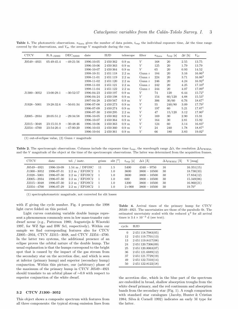
Table 1. The photometric observations. ndata gives the number of data points, texp the individual exposure time, ∆t the time rangecovered by the observations, and Vav the average V magnitude during the run.

CTCV R.A.J2000 DECJ2000 date HJD telescope filter ndata texp [s] ∆t [h] Vav

J0549−4921 05:49:45.4 −49:21:56 1996-10-05 2 450 362 0.9 m V 168 20 2.55 13.751996-10-06 2 450 363 0.9 m V 125 20 1.79 13.791996-10-07 2 450 364 0.9 m V 65 20 0.93 14.521998-10-31 2 451 118 2.2 m Gunn r 184 20 3.16 16.862

1998-11-01 2 451 119 2.2 m Gunn r 224 20 3.71 16.862

1998-11-02 2 451 120 2.2 m Gunn r 246 20 4.24 16.922

1998-11-03 2 451 121 2.2 m Gunn r 242 20 4.25 17.102

1998-11-04 2 451 122 2.2 m Gunn r 244 20 4.07 17.092

J1300−3052 13:00:29.1 −30:52:57 1996-04-23 2 450 197 0.9 m V 74 120 6.44 15.721

1996-04-24 2 450 198 0.9 m V 154 60/120 4.88 15.531

1997-04-28 2 450 567 0.9 m V 306 30/60 6.76 18.671

J1928−5001 19:28:32.6 −50:01:34 1996-07-08 2 450 273 0.9 m V 55 240/80 3.09 17.791

1996-07-09 2 450 274 0.9 m V 197 60 5.21 17.871

1996-07-30 2 450 295 2.2 m V 47 15/120 3.12 17.801

J2005−2934 20:05:51.2 −29:34:58 1996-10-05 2 450 362 0.9 m V 169 30 2.90 15.911996-10-07 2 450 364 0.9 m V 164 30 2.81 15.92

J2315−3048 23:15:31.9 −30:48:46 1996-10-06 2 450 363 0.9 m V 124 60 3.14 16.831

J2354−4700 23:54:20.4 −47:00:20 1996-10-03 2 450 360 0.9 m V 24 240 1.78 18.871

1996-10-04 2 450 361 0.9 m V 66 180 3.83 19.021

(1) out-of-eclipse value, (2) Gunn r magnitude

Table 2. The spectroscopic observations. Columns include the exposure time texp, the wavelength range ∆λ, the resolution ∆λFWHM,and the V magnitude of the object at the time of the spectroscopic observations. The latter was determined from the acquisition frames.

CTCV date tel. / instr. grism slit [′′] texp [s] ∆λ [A] ∆λFWHM [A] V [mag]

J0549−4921 1996-10-09 1.54 m / DFOSC 11 1.5 5400 4340 – 9750 16 16.351(15)J1300−3052 1996-07-31 2.2 m / EFOSC2 1 1.0 3600 3800 – 10500 30 18.730(33)J1928−5001 1996-07-30 2.2 m / EFOSC2 1 1.0 3600 3800 – 10500 30 17.834(12)J2005−2934 1996-07-30 2.2 m / EFOSC2 1 1.0 600 3800 – 10500 30 15.349(06)J2315−3048 1996-07-30 2.2 m / EFOSC2 1 1.0 1200 3800 – 10500 30 16.960(21)J2354−4700 1996-07-29 2.2 m / EFOSC2 1 1.0 2×900 3800 – 10500 30 19.701

(1) spectrophotometric magnitude, not corrected for slit losses

with E giving the cycle number. Fig. 4 presents the 1998light curve folded on this period.

Light curves containing variable double humps repre-sent a phenomenon commonly seen in low mass-transfer ratedwarf novae (e.g., Patterson 1980; Augusteijn & Wisotzki1997, for WZ Sge and BW Scl, respectively). Within oursample we find corresponding features also for CTCVJ2005−2934, CTCV J2315−3048, and CTCV J2354−4700.In the latter two systems, the additional presence of aneclipse proves the orbital nature of the double hump. Theusual explanation is that the humps correspond to the brightspot that is caused by the impact of the gas stream fromthe secondary star on the accretion disc, and which is seenat inferior (primary hump) and superior (secondary hump)conjunction. Within this picture, our (arbitrary) phase ofthe maximum of the primary hump in CTCV J0549−4921should translate to an orbital phase of ∼0.8 with respect tosuperior conjunction of the white dwarf.

3.2 CTCV J1300−3052

This object shows a composite spectrum with features fromall three components: the typical strong emission lines from

Table 4. Arrival times of the primary hump for CTCVJ0549−4921. The uncertainties are those of the parabolic fit. Theestimated uncertainty scaled with the reduced χ2 for all arrivaltimes is 3.4× 10−3 d (see text).

cycle HJD

0 2 451 118.7983(05)12 2 451 119.7701(13)13 2 451 119.8417(08)24 2 451 120.7306(09)25 2 451 120.8063(07)36 2 451 121.6889(12)37 2 451 121.7729(19)49 2 451 122.7310(14)50 2 451 122.8122(18)

the accretion disc, which in the blue part of the spectrumare embedded in broad, shallow absorption troughs from thewhite dwarf primary, and the red continuum and absorptionbands from the secondary star (Fig. 1). A rough comparisonwith standard star catalogues (Jacoby, Hunter & Cristian1984; Silva & Cornell 1992) indicates an early M type forthe latter.

c© 0000 RAS, MNRAS 000, 000–000

4 C. Tappert et al.

Figure 1. Spectra of the 6 CTCV sources as indicated. The absorption feature at λ7440 for CTCV J2354−4700 is an artifact.

We have observed the system photometrically in twodifferent years, which proved it to be in a state of increasedbrightness during the first observing run in 1996. The lightcurves of both runs are given in Fig. 5. It shows the systemwith a ∼3 mag deep eclipse in quiescence. In the system’shigh state the eclipse depth is diminished to ∼1.1 mag.

We have fitted second order polynomial functions tothe eclipse data in order to determine the times of mid-eclipse. The results are given in Table 5. Unfortunately, a

period analysis could not be performed on the combineddata set, since the time span between the two observing runsproved too large for an unambiguous cycle count. Linear fitsto the mid-eclipse timings for the individual runs yielded theephemerises

T0 = HJD 2 450 197.565 33(26) + 0.088 981(32) E, (2)

for the 1996 data, and

c© 0000 RAS, MNRAS 000, 000–000

Cataclysmic variables from the Calan-Tololo Survey. I. 5

Table 3. Equivalent widths (in A) of the most prominent emission lines. A blank field indicates that this part of the spectrum was notcovered with our observations, a ‘−’ that the corresponding line was not detected.

CTCV Balmer He I He II Fe II4102 4340 4861 6563 4471 5016 5876 6678 7065 4686 5173

J0549−4921 35 52 6 4 11 5 – 8 6J1300−3052 15 24 47 110 – – 12 – – – –J1928−5001 – – 13 11 – – – – – – –J2005−2934 25 33 66 219 6 8 18 5 9 – 8J2315−3048 31 44 45 102 14 11 32 11 11 9 6J2354−4700 13 41 58 104 22 21 40 21 18 – –

Figure 2. Light curves for the 1996 data of CTCV J0549−4921.Note that the relative magnitude range is the same for all plots.

T0 = HJD 2 450 567.559 19(29) + 0.088 85(24) E, (3)

for the 1997 data, with E giving the cycle number. Withinthe errors, both periods are consistent with each other. Thisperiod places the system close to the lower edge of the CVperiod gap (e.g. Fig. 13 in Tappert & Bianchini 2003).

The quiescence data folded on its ephemeris shows a‘classical’ shape of a broad hump prior to eclipse (Fig. 6),very similar e.g. to that of U Gem (Krzeminski 1965). Theoutburst light curve shows large, apparently irregular, vari-ations from cycle to cycle (Fig. 7). A noteworthy feature ofthese data is the smaller depth and the larger width of theeclipse with respect to the quiescence data (∼ 1 mag and30 min for the full eclipse width compared to ∼ 3 mag and

Figure 3. Light curves for the 1998 data of CTCV J0549−4921.

19 min), as a consequence of increased disc luminosity andradius.

A more detailed study of the eclipse light curve andadditional follow-up spectroscopic observations will be pub-lished elsewhere (Augusteijn et al., in preparation).

3.3 CTCV J1928−5001

The spectrum of this object (Fig. 1) also shows contributionsfrom multiple components. In the red part we see the signa-tures of the secondary star whose spectral type appears to beslightly later than M5V (Jacoby et al. 1984). The blue partis dominated by the Balmer absorption lines from the whitedwarf primary. The source was identified as a Polar (or AM

c© 0000 RAS, MNRAS 000, 000–000

6 C. Tappert et al.

Figure 4. Light curve for CTCV J0549−4921 folded on P =0.080 239 d. The zero point of the phase has been set to the firstdata point. The symbols in the upper plot refer to the individualdata sets from 1998-10-31 (◦), 11-01 (✷), 11-02 (△), 11-03 (×),and 11-04 (✸). The error bars from phase 0 to 1 correspond to thephotometric error as in Fig. 3. The lower plot shows the averagelight curve. The bin size is 0.05 phases.

Figure 5. Light curves for CTCV J1300−3052 from 1996-04-23(top), 1996-04-24 (middle), and 1997-04-28 (bottom). Note thatthe y-axis of the bottom plot has a different scale.

Table 5. Eclipse timings for CTCV J1300−3052. Due to the cycleambiguity between both data sets, each refers to its individualzero point. The estimated error scaled by the reduced χ2 for the1996 data amounts to 3.4× 10−4 d. For the 1997 data, the errorsresulting from the parabolic fit already gave reasonable residuals.

cycle HJD

1996:0 2 450 197.565 12(05)2 2 450 197.743 57(06)

11 2 450 198.543 86(08)12 2 450 198.633 29(08)

1997:0 2 450 567.559 19(35)1 2 450 567.648 05(22)2 2 450 567.736 90(34)

Figure 6. The 1997 light curve for CTCV J1300−3052 folded onthe ephemeris given in Eq. 3.

Figure 7. Phase folded outburst data CTCV J1300−3052 withrespect to the ephemeris given in Eq. 2. Different symbols indicatedifferent orbital cycles: ◦, ✷, △, ⋄, for cycles −1, 0, 1, 2 (1996-04-23), and dot, +, ×, for cycles 10, 11, 12 (1996-04-24), respectively.

c© 0000 RAS, MNRAS 000, 000–000

Cataclysmic variables from the Calan-Tololo Survey. I. 7

Figure 8. Out-of-eclipse (left) and mid-eclipse (right) V imageof CTCV J1928−5001 from 1996-07-30.

Figure 9. Light curve of CTCV J1928−5001 from 1996-07-09.The magnitudes represent the combined data from the CV andits close visual companion (V = 18.5)

Her) type CV by follow-up spectroscopic and polarimetricobservations which will be published elsewhere (Potter etal., in preparation).

The object is a close visual binary with a separation ≈2.′′4. Additionally, the CV is a deeply eclipsing system (Figs.8, 9). Mid-eclipse photometry of the companion gave V =18.52(1) mag, yielding out-of-eclipse values for the CV of V= 17.7–18.0 mag. In order to estimate the mid-eclipse mag-nitude of the target, we subtracted the average PSF fromthe companion on an eclipse frame. Aperture photometryon the residual yielded V = 21.05(30). Note, however, thatthe error is a purely photometric one, and does not take intoaccount uncertainties in the PSF fitting or in the time devi-ation from true mid-eclipse, especially since the exact shape

Table 6. Eclipse timings for CTCV J1928−5001 as measuredwith a polynomial fit of second order. The estimated uncertaintyscaled by the reduced χ2 is 1.8× 10−4 d.

cycle HJD

−15 2 450 273.728 37(14)−14 2 450 273.798 92(08)−1 2 450 274.711 02(15)0 2 450 274.781 39(08)1 2 450 274.851 29(16)

297 2 450 295.624 47(09)298 2 450 295.694 26(06)

Figure 10. All three light curves of CTCV J1928−5001 foldedon the ephemeris given in Eq. 4. The upper plots shows the dif-ferential magnitudes (the CV plus companion) to give an idea ofthe brightness variations of the system in its low state. The lowerplot represents a close-up of the out-of-eclipse data.The latterlight curves have been normalised individually by subtracting thecorresponding out-of-eclipse average magnitude. In both plots thesymbols × and △ from phases 1 to 2 refer to the 1996-07-08 and1996-07-30 data, respectively, while the dots represent the 1996-07-09 data. The error bars from phases 0 to 1 correspond to theindividual photometric errors.

of the eclipse light curve is unknown. Therefore, deep mid-eclipse photometry will be needed to accurately determinethe eclipse depth.

A linear fit to the timings of mid-eclipse (Table 6)yielded an ephemeris

T0 = HJD 2 450 274.781 24(08) + 0.070 179(01) E, (4)

with the error of the zero cycle referring to the error ofthe linear regression. Fig. 10 shows the corresponding lightcurve.

3.4 CTCV J2005−2934

Although the spectrum of this system displays all basic in-gredients of a typical dwarf nova, it is peculiar in that itsHα line is unusually strong, especially in comparison to theother Balmer lines (Fig. 1, Table 3).

The photometric data was taken in two nights, witheach data set spanning a very similar time range. Thelight curves are presented in Fig. 11. Other than in the

c© 0000 RAS, MNRAS 000, 000–000

8 C. Tappert et al.

Figure 11. Light curves for CTCV J2005−2934 from 1996-10-05(top) and 1996-10-07 (bottom).

Table 7. Frequencies f , corresponding periods P , and the dis-criminatory power pd from the Monte Carlo simulation on theCTCV J2005−2934 data.

f [cyc d−1] P [d] pd ID

14.901(15) 0.067 111(69) 0.000 P1

15.398(05) 0.064 943(21) 0.091 P2

15.902(09) 0.062 887(37) 0.637 P3

16.401(04) 0.060 972(14) 0.272 P4

16.892(07) 0.059 200(25) 0.000 P5

CTCV J0549−4921 data, the time range and the numberof covered humps are insufficient to use the arrival timesof the principal hump to derive the period. Additionallythe hump appears less constant in shape than the one ofCTCV J0549−4921. After subtracting the nightly averages,we therefore applied the AOV algorithm to the combineddata set. The corresponding periodogram shows a numberof sharp peaks centred on f ∼16 cyc d−1. For our MonteCarlo simulation we compared the five highest peaks. Thecorresponding frequencies and the resulting discriminatorypower for a specific frequency over the other four are listed

Figure 12. AOV periodogram for the CTCV J2005−2934 data.The inlet shows a close-up of the main peaks.

Figure 13. Normalised light curve for CTCV J2005−2934 foldedon P = 0.062 887 d. The zero point of the phase has been set tothe first data point. The symbols in the upper plot refer to theindividual data sets from 1996-10-05 (×) and 1996-10-07 (✷). Theerror bars from phase 0 to 1 correspond to the photometric erroras in Fig. 11. The lower plot shows the average light curve. Thebin size is 0.05 phases.

in Table 7. Thus, P3 emerges as the most probable period,while we can certainly discard P1 and P5. However, espe-cially P4 still represents an important alias, and additionalobservations will be necessary to properly assign the orbitalperiod.

In Fig. 13 we present individual light curves and theaverage one folded on the most probable period P3. Phase-folding on P2 or P4 yields very similar scatter and basicallyidentical phasing of the main features. The light curve is inprinciple similar to that of CTCV J0549−4921 in that it con-sists of two humps of different size. Their amplitudes, how-ever, are only half as strong as those in CTCV J0549−4921,which could mean that CTCV J2005−2934 is seen at a some-what lower inclination. Using the same interpretation for thenature of these humps, orbital phase ∼0.8 should correspondto our arbitrary phase 0.03 for the maximum of the primaryhump.

3.5 CTCV J2315−3048

This object shows a very typical spectrum of a dwarf nova inquiescence with strong emission lines of the H and He series(Fig. 1, Table 3). It has been independently discovered asthe ROSAT source 1RXS J231532.3−304855 (Schwope et al.2000) and in the Edinburgh-Cape Blue Object Survey asEC 23128−3105 (Chen et al. 2001). The latter authors de-rive an orbital period P = 0.0584(2) d from time-resolvedspectroscopy. They furthermore find a strong orbital modu-lation in a photometric light curve from 1991, and report apossibly transient feature resembling a shallow eclipse.

We have observed the system in one night 5 yearslater, with the data set covering roughly 2.25 orbital cy-cles. The light curve is presented in Fig. 14. The AOV pe-riodogram yields two broad peaks corresponding to P andP/2. Since with our data set we cannot obtain the accuracyof Chen et al. (2001) in the period determination, we haveused their value to compute a phase-folded light curve (Fig.15).

c© 0000 RAS, MNRAS 000, 000–000

Cataclysmic variables from the Calan-Tololo Survey. I. 9

Figure 14. Light curve for CTCV J2315−3048 from 1996-10-06.

Figure 15. Light curve for CTCV J2315−3048 folded on theephemeris given in Eq. 5. The data have been normalised by sub-tracting a polynomial of second order. For the fit the eclipse dataand the first hump were excluded. The data set in the upper plothas been divided into three parts, each corresponding to a dif-ferent orbital cycle (−2 = ×, −1 = ✷, 0 = △). The error barsfrom phase 0 to 1 correspond to the photometric error as in Fig.14. The lower plot shows the average light curve with a bin sizeof 0.05 phases. The y-scale has been set in such a way to enabledirect comparison to Fig. 3 of Chen et al. (2001).

The presence of strong flickering has a distorting effectwithin an individual orbital cycle. However, in our averagelight curve we find the same principal features as in Chenet al.’s data (their Fig. 3). Of special interest is that wealso detect an eclipse-like dip just after the primary maxi-mum. Chen et al. report that this feature is not found in alltheir light curves. Also in our data the first eclipse featureis much less evident than the second one. By simply takingthe average in time for the two data points that define thesecond eclipse, and which have the same magnitude withinthe errors, we obtain an ephemeris

T0 = HJD 2 450 363.711 90(53) + 0.058 4(2) E, (5)

with the periodic term taken from (Chen et al. 2001). Theerror for the zero cycle corresponds to half of the separationof the two data points, and is therefore likely to be somewhatoverestimated.

Figure 16. Light curves for CTCV J2354−4700 from 1996-10-03(top) and 1996-10-04 (bottom).

Table 8. Times of mid-eclipse for the CTCV J2354−4700 data.

cycle HJD

0 2 450 360.661 45(56)16 2 450 361.709 80(47)17 2 450 361.775 80(46)

3.6 CTCV J2354−4700

The spectrum of this object is very similar to the one ofCTCV J2315−3048, i.e. of a dwarf nova in quiescence (Fig.1).

CTCV J2354−4700 was observed on two subsequentnights. Fig. 16 presents the resulting light curves, and Ta-ble 8 lists the times of mid-eclipse which were obtained byfitting a second order polynomial to the eclipse data.

A linear fit to these times yielded the ephemeris

T0 = HJD 2 450 360.661 43(56) + 0.065 538(39) E. (6)

Figure 17. The 1996-10-04 light curve of CTCV J2354−4700folded on the ephemeris given in Eq. 6. The symbols in the plotrefer to different orbital cycles (15 = ×, 16 = ✷, 17 = △). Thedata have been normalised by subtracting a linear fit to the data(excluding humps and eclipses) with a slope of 2.59 mag d−1.

c© 0000 RAS, MNRAS 000, 000–000

10 C. Tappert et al.

Table 9. Summary of the orbital periods for the six CVs.

object P [d] P [h] notes

CTCV J0549−4921 0.080 218(70) 1.9252(17)CTCV J1300−3052 0.088 981(32) 2.135 54(77) [1]CTCV J1928−5001 0.070 179(01) 1.684 296(24) [1]CTCV J2005−2934 0.062 887(37) 1.5093(09) [2]CTCV J2315−3048 0.058 4(2) 1.402(05) [1], [3]CTCV J2354−4700 0.065 538(39) 1.5729(09) [1]

[1] eclipsing, [2] most probable alias, [3] period fromChen et al. (2001)

Both data sets for CTCV J2354−4700 show steadilydeclining light curves. Linear fits, excluding the humps andeclipses, yielded slopes of 1.05(49) mag d−1 and 2.59(24)mag d−1 for the 1996-10-03 and the 1996-10-04 data, respec-tively. Since on both dates the average magnitudes are verysimilar, it is clear that at least the value for the first nightdoes not reflect the system’s behaviour over a longer periodof time. Therefore, either the CV has undergone some slow,non-orbital, variations between the two nights, or the decline(perhaps in both nights) is artificial. For the 1996-10-04 datathe airmass has been continuously increasing (from 1.05 to1.58), and 3 of the 5 stars in the average comparison lightcurves are very red with B − V > 0.9, raising the suspicionthat the decline may be due to differential extinction. How-ever, light curves for the target computed with respect to thebluest (B−V = 0.4) and the reddest (B−V = 1.5) compar-ison star yield nearly identical decline rates. Computing thedifference light curve of the two comparison stars with themost extreme colour coefficient we do find the signature ofdifferential extinction in the form of a decline of ∼0.1 magd−1 for both nights (in the first night, the standard devia-tion of the slope even still includes a constant light curve).In the average light curve, this effect can be assumed to beeven less pronounced. We therefore do not find any indica-tion for an artificial origin of the observed decline, but dueto the rather limited amount of data we have to leave thequestion on the cause of this apparent long-term variationto be answered by future studies.

In order to fold the data on the above ephemeris,we have subtracted the linear decline from the 1996-10-04data. Fig. 17 presents the such normalised, phase-folded,light curve. Its shape is very similar to that of CTCVJ1300−3052, although in the latter both the amplitudeof the hump and the depth of the eclipse are roughlytwice as strong, suggesting a lower inclination for CTCVJ2354−4700.

4 SUMMARY

We have presented the results of time-series photometry forsix CVs that were detected in the Calan-Tololo Survey, andwhere we find photometric variations that we believe to bemodulated with the orbital period. For five of the systems wederived this previously unknown period, and in the case ofCTCV J2315−3048 we have confirmed the existence of aneclipse, which has been previously discussed as a possiblytransient feature Chen et al. (2001). The resulting periodsfor all systems are summarised in Table 9.

ACKNOWLEDGEMENTS

This research is based on observations made at ESO, pro-posal numbers 57.D-0704, 58.D-0551, 58.D-0549, 59.D-0368.It has made use of the SIMBAD database, operated at CDS,Strasbourg, France. The Digitized Sky Surveys were pro-duced at the Space Telescope Science Institute under U.S.Government grant NAG W-2166, based on photographicdata obtained using the Oschin Schmidt Telescope on Palo-mar Mountain and the UK Schmidt Telescope. IRAF is dis-tributed by the National Optical Astronomy Observatories.We thank the anonymous referee for helpful comments.

REFERENCES

Andronov N., Pinsonneault M., Sills A., 2003, ApJ, 582,358

Augusteijn T., Wisotzki L., 1997, A&A 324, L57Barker J., Kolb U., 2003, MNRAS, 340, 623Bessell M. S., 1990, PASP, 102, 1181Chen A., O’Donoghue D., Stobie R. S., Kilkenny D.,Warner B., 2001, MNRAS, 325, 89

Echevarrıa J., 1984, Rev. Mex. Astron. Astrof., 9, 99Gansicke B.T., Hagen H.-J., Engels D. 2002, in GansickeB. T., Beuermann K., Reinsch K., eds, The Physics ofCataclysmic Variables and Related Objects, ASP Conf.Ser., 261, p. 190

Green R. F., Schmidt M., Liebert J., 1986, ApJS, 61, 305Howell S. B., Rappaport S., Politano M., 1997, MNRAS,287, 929

Jacoby G. H., Hunter D. A., Cristian C. A., 1984, ApJS,56, 257

King A. R., Schenker K., 2002, in Gansicke B. T., Beuer-mann K., Reinsch K., eds, The Physics of CataclysmicVariables and Related Objects, ASP Conf. Ser., 261, p.233

Kolb U., 1993, A&A, 271, 149Kolb U., Baraffe I., 1999, MNRAS, 309, 1034Krzeminski W., 1965, ApJ, 142, 1051Landolt A. U., 1992, AJ, 104, 340Marsh T. R., 2000, New Astron. Rev., 44, 119Maza J., Ruiz M. T., Gonzalez L. E., Wischnjewsky M.,1989, ApJS, 69, 349

Mennickent R.E., Tappert C., 2001, A&A 372, 563Patterson J., 1980, ApJ, 241, 235Patterson J., 1984, ApJS, 54, 443Patterson J., 1998, PASP, 110, 1132Ritter H., Kolb U., 2003, A&A, 404, 301Schwarzenberg-Czerny A., 1989, MNRAS, 241, 153Schwope A., Hasinger G., Lehmann I., et al., 2000, Astron.Nachr., 321, 1

Shara M.M., Livio M., Moffat A. F. J., Orio M., 1986, ApJ,311, 163

Silva D. R., Cornell M. E., 1992, ApJS, 81, 865Spruit H. C., Taam R. E., 2001, ApJ, 548, 900Stehle R., Kolb U., Ritter H., 1997, A&A, 320, 136Stetson P. B., 1992, in Worrall D. M., Biemesderfer C.,Barnes J., eds, Astronomical Data Analysis Software andSystems I, ASP Conf. Ser., 25, p.291

Stobie R. S., Kilkenny D., O’Donoghue D., et al., 1997,MNRAS, 287, 848

c© 0000 RAS, MNRAS 000, 000–000

Cataclysmic variables from the Calan-Tololo Survey. I. 11

Szkody P., Anderson S. F., Agueros M., et al., 2002, AJ,123, 430

Szkody P., Fraser O., Silvestri N., et al., 2003, AJ, 126,1499

Tappert C., Bianchini A. 2003, A&A, 401, 1101Tappert C., Augusteijn T., Maza J., 2002, in Gansicke B.T., Beuermann K., Reinsch K., eds, The Physics of Cat-aclysmic Variables and Related Objects, ASP Conf. Ser.,261, p.299

Warner B., 1995, Cataclysmic Variable Stars, CambridgeUniversity Press

APPENDIX A: FINDING CHARTS

We here present 5′×5′ finding charts for the 6 CVs.

c© 0000 RAS, MNRAS 000, 000–000

12 C. Tappert et al.

Figure A1. Finding charts from the Digitized Sky Survey.

c© 0000 RAS, MNRAS 000, 000–000