1

Photo-Consistent Reconstruction ofSemi-Transparent Scenes by Density Sheet

DecompositionSamuel W. Hasinoff, Student Member, IEEE, and Kiriakos N. Kutulakos, Member, IEEE

Abstract— This article considers the problem of reconstructingvisually realistic 3D models of dynamic semi-transparent scenes,such as fire, from a very small set of simultaneous views (eventwo). We show that this problem is equivalent to a severelyunder-constrained computerized tomography problem, for whichtraditional methods break down. Our approach is based on theobservation that every pair of photographs of a semi-transparentscene defines a unique density field, called a Density Sheet,that (1) concentrates all its density on one connected, semi-transparent surface, (2) reproduces the two photos exactly, and(3) is the most spatially compact density field that does so.From this observation, we reduce reconstruction to the convexcombination of sheet-like density fields, each of which is derivedfrom the Density Sheet of two input views. We have applied thismethod specifically to the problem of reconstructing 3D modelsof fire. Experimental results suggest that this method enableshigh-quality view synthesis without over-fitting artifacts.

Index Terms— Semi-transparent scenes, fire, volumetric re-construction, 3D reconstruction, computerized tomography, viewsynthesis, image-based modeling, image-based rendering.

I. INTRODUCTION

THE computational modeling of physical phenomena such

as fire and smoke has received significant attention

in computer graphics [1]–[8] as well as in other fields of

experimental science [9]–[16]. While photographs provide a

great deal of information about such phenomena, very little is

known about how 3D models can be extracted from images.

Extracting such information could open up new opportunities

for creating better visual models [1], [2], [4], [6]; developing

image-based representations of such phenomena [17]; per-

mitting the manipulation of scene appearance in photographs

that contain such phenomena; and developing new, dynamic

simulation systems that use real-world data as input.

Toward this end, this article considers the problem of recon-

structing semi-transparent scenes from a set of simultaneously-

captured images or videos. We take fire as our central example,

and show that by using optical models developed in the

combustion literature [10], [11], [18], we can model fire as a

semi-transparent density field whose appearance at a projected

The authors are with the Department of Computer Science, University ofToronto, Canada, M5S 3G4. Email: {hasinoff,kyros}@cs.toronto.edu.

Manuscript received May 31, 2005; revised January 27, 2006; acceptedJuly 11, 2006.

The authors gratefully acknowledge the support of the National ScienceFoundation under Grant No. IRI-9875628, of the Natural Sciences andEngineering Research Council of Canada under the RGPIN, PGS-A, and CGS-D programs, and of the Alfred P. Sloan Foundation.

pixel is a linear function of the transparencies along the

corresponding ray.

We believe that any practical method for modeling dynamic

semi-transparent scenes from multiple viewpoints must satisfy

three criteria:

• Small viewpoint coverage: Dynamic phenomena require

simultaneous image capture. While multi-view systems

with tens of video cameras do exist [11], [19], the method

should not break down for small datasets.

• Photo-consistency: To preserve visual realism, recon-

structed density fields must reproduce the input images.

• Good view synthesis: All views should be rendered with

high quality, without “over-fitting” the limited number of

input views.

Even though these criteria have received much attention in

the case of opaque objects [19], satisfying them for semi-

transparent scenes is not well understood.

At the heart of our approach lies the observation that every

pair of photos of a semi-transparent scene uniquely determines

two special density fields, called Density Sheets, each of

which reproduces the photographs exactly and concentrates

all its density along a single connected surface. Using this

observation as a starting point, we show the following: (1)

Density Sheets can be decomposed into a family of solutions

involving further sheet-like structures, (2) this family is a basis

of the space of density fields that are photo-consistent with two

or more views, and (3) the space of photo-consistent density

fields is linear and convex. These results lead to a simple and

efficient algorithm, called Density-Sheet Decomposition, that

computes the density field as a convex combination of sheet-

like density fields derived from pairs of input views.

Unlike existing methods for reconstructing semi-transparent

scenes, Density-Sheet Decomposition is specifically designed

to capture models that are both photo-consistent and have

good view synthesis capabilities. Intuitively, Density Sheets

represent the most spatially-compact interpretation of the input

views. Moreover, Density Sheets are unique and lead to a re-

construction method that is well-posed and easy to implement.

This allows us to reconstruct semi-transparent scenes from as

few as two input views, while also being able to incorporate

more views if they are available.

Our approach offers five contributions over the existing

state of the art. First, unlike methods where photo-consistency

and spatial smoothness are the only objectives [20]–[23], our

0000–0000/00$00.00 c© 2006 IEEE

2

approach establishes spatial compactness as another objective

for visual reconstruction. Second, it leads to a well-posed

reconstruction algorithm that can handle any number of input

views. Third, it introduces Density Sheets as a complete

basis for the space of photo-consistent density fields, enabling

their potential use for reconstructing and rendering any semi-

transparent scene where the linear image formation model is

valid. Fourth, the sheet-like structure of the Density-Sheet

Decomposition algorithm enables use of simple warp-based

methods [24] to create photo-realistic views of the recon-

structed scene. Fifth, our results on fire datasets show that the

algorithm is able to render detailed reconstructions of complex

flames without over-fitting artifacts.

We begin this article by discussing the relation of this

work to current approaches for reconstructing semi-transparent

scenes in general and fire in particular. In Section III we

present a simplified imaging model for fire, which establishes

an equivalence between fire reconstruction and computerized

tomography. Because of this equivalence, the rest of our

analysis applies to the general case of semi-transparent scenes

(Section IV). In Section V we present an analysis of the

space of density fields photo-consistent with two views, and

introduce the Density Sheet solution. We then generalize the

analysis to multiple views, and describe several properties that

allow us to reduce the problem to the two-view case (Sec-

tion VI). In Section VII we describe a new family of photo-

consistent density fields built from sheet-like structures, and

show that this family can be used to represent arbitrary density

fields. This leads to an algorithm for M -view photo-consistent

reconstruction that models density fields as superpositions of

sheets. In Section VIII we present experimental results using

real images of fire. We conclude with a discussion of our

approach and some proposed directions for future work.

II. RELATED WORK

The 3D modeling of fire and other semi-transparent scenes

has received significant attention in computer graphics. Both

physics-based [1]–[3], [5] and procedural [6]–[8] models have

been used to produce visually realistic simulations of torches,

gaseous jets of flame, and smoke. For scenes consisting of

strongly-scattering particles such as smoke, high-fidelity 3D

capture of real scenes has been shown using laser illumination

and high-speed photography [4]. But the question of how

we can capture models of general semi-transparent scenes,

particularly from standard images, remains largely open.

In addressing this question we touch upon four distinct lines

of work: computerized tomography, volumetric reconstruction

in computer vision, combustion measurement, and 2D image-

based modeling for dynamic scenes.

A. Reconstructing Semi-Transparent Scenes

1) Computerized Tomography: The problem of reconstruct-

ing semi-transparent scenes has received the most attention

in the context of computerized tomography. Our interest is

in using very few views (two or more), which is closest

to the “sparse-view tomography” problem. Some sparse-view

methods produce a binary segmentation rather than a full

reconstruction [25]–[27] and, in the context of tomography,

“sparse” can actually mean eight or more views [21], [23],

[25]. On the other hand, classic methods such as filtered back-

projection and algebraic techniques (e.g., [20], [28]) require

tens or hundreds of input views for accurate results.

Tomography methods that are specialized to the ill-posed

nature of the sparse-view case use various techniques to regu-

larize the problem. This includes favoring local smoothness

in a statistical framework [21], [27], assuming prior shape

models [25]–[27], and coarsely discretizing the density levels

[21]. Unfortunately, these methods still break down when the

number of views is extremely limited and fail to generate 3D

reconstructions adequate for photo-realistic view synthesis.

2) Volumetric Reconstruction in Computer Vision: In the

stereo vision literature, several volumetric methods have at-

tempted to recover transparencies along with voxel color

information [22], [29], [30]. While some of these methods are

more directed at modeling occlusion uncertainty [30] or mixed

pixels at object boundaries [22], several of these methods

have addressed the full tomography problem [22], [29]. For

example, the Roxel method [29] is related to algebraic methods

from computerized tomography [20] but its imaging model

has an unclear physical basis since it confounds transparency

and uncertainty. These methods do not guarantee photo-

consistency, nor do they produce results suitable for view

synthesis, particularly when the number of views is limited.

Along similar lines, algebraic methods from tomography

have also been applied to image-based rendering for trees with

dense foliage, from tens of views [31]. Because a significant

fraction of pixels in this context are opaque, this approach is

closer to view-dependent texture mapping using the visual hull

and is less suitable for complex semi-transparent scenes that

consist of multiple layers.

Although methods for reconstructing semi-transparent

scenes from a sparse number of views have attempted to

address the ill-posed nature of the problem, none of the above

methods explicitly characterize the fundamental ambiguities

in the space of photo-consistent solutions. For this reason,

they are ill-equipped for handling the extreme cases (i.e., two

views). To our knowledge, the only previous work addressing

tomographic reconstruction with two views involves binary

density fields for segmentation [27].

B. Reconstructing Fire

1) Combustion Measurement: In the combustion literature,

methods for the 3D measurement of fire have mainly been di-

rected toward the measurement of specific physical properties

(e.g., temperature) and the qualitative recovery of 3D shape

[9]–[16]. Most methods do not restrict themselves to visible

light images from cameras, but rather employ a wide variety

of sensors. Common approaches involve lasers [11], [16],

special optical systems to exaggerate refraction [11]–[15],

and thermography devices [9], [10]. None of these methods

provide instantaneous 3D reconstruction at resolutions high

enough for image-based rendering. In fact, many previous

methods capture images with multiple-second exposures [9],

[10], [12], [15] or assume a “stationary” fire [11] to reconstruct

3

rough approximations to the density field. As a result, these

methods are not appropriate for view synthesis and cannot be

used to model complex flickering flames (e.g., Fig. 11), whose

structures can change dramatically from instant to instant.Because the straightforward application of classic tomogra-

phy methods [20], [28] to fire reconstruction would require

an impractical number of synchronized cameras, results in

this vein have been severely limited in both resolution and

accuracy [9], [13], [32]. One exception is a twenty-camera

apparatus designed to reconstruct quasi-static or non-visible

flame [11]. More recently, methods from sparse-view tomog-

raphy have been applied to fire reconstruction as well using

eight synchronized cameras [23]. While this approach yields

a plausible density distribution at a scale coarser than a pixel,

the high-frequency detail present in the original images is

not reconstructed. For an extremely limited number of views

(e.g., 2–5), even such sparse-view tomography methods fail

to produce results appropriate for view synthesis [21], [23],

[25]–[27].2) Image-Based Modeling for Dynamic Scenes: An alterna-

tive approach is to avoid almost all reconstruction and model

fire in strictly image-based terms. Image-based methods such

as video textures [17], [33] and linear dynamical systems [34],

[35], have already been applied to fit simple 2D dynamic

models of fire to video sequences. Although these methods

can generate realistic continuations of flickering flames, and

even allow basic attributes such as speed [35] and direction

of flow [36] to be manipulated, they do not allow us to vary

viewpoint nor to model non-stationary effects such as materials

consumed by fire.

III. LINEAR OPTICAL MODEL OF FIRE

Fire is typically defined as an oxygen-fueled chemical

decomposition that releases heat to the environment [18]. In

this work we are strictly concerned with flames, i.e., the

visible luminous reaction products of fire.1 We rely on a first-

order model of flame appearance, proposed in the combustion

measurement literature, called the soot volume model [18].

Under this model, the appearance of flame is generated by a

continuum of luminous carbonaceous soot particles, where in

a given infinitesimal volume, both intensity and absorption are

proportional to soot particle density. Following the approach

of Stam [2], we ignore refraction2 and derive this model as a

specialization of a more general model for radiative transfer

[37].At a given image point, the image irradiance, I , can be

expressed as the sum of two terms—a term that integrates

radiance from luminous fire material along the ray through

that pixel and a term that incorporates background radiance

(Fig. 1):

I =

∫ L

0

D(t) τ(t)J(t) dt + Ibgτ(L), (1)

1In general, not all fire burns with visible flames. Some gases that burncleanly are visually detectable only by their secondary effects, for examplethe refractive distortion of the atmosphere [11]. We do not deal with this typeof fire here.

2The combustion literature supports this assumption, as the refraction invisible flame is generally small, with deflections less than 0.1◦ [11], [14].

cbgI D t( )

t• • • •

L

fire density fieldplaneimage

I

Fig. 1. Optical model of fire. The image irradiance, I , at a pixel dependson the integral of luminous fire density along a ray through the center ofprojection, c. The density field, D(t), along the ray is parameterized by the

distance, t ∈ [0, L], from the image plane. The background intensity, Ibg ,

also contributes to the intensity, I .

where D(t) is the fire’s density field along that ray; J models

the total effect of emission and in-scatter less any out-scatter

per unit mass; L defines the interval [0, L] along the ray where

the field is non-zero; Ibg is the radiance of the background;

and τ models transparency. The transparency can be thought

of as the degree by which the fire products between the pixel

and a position x along the ray permit the radiance from further

away to reach that pixel,

τ(x) = exp

(

−σ

∫ x

0

D(t) dt

)

, (2)

where σ is a positive medium-dependent constant known as

the extinction cross-section [18], and is assumed to be constant

throughout the fire.

To simplify this model, we rely on two further assumptions

used in the combustion literature:

• Negligible scattering: This is a good approximation

for fire not substantially obscured by smoke because

emission from luminous soot particles dominates radiance

[2], [10], [11], [14]. In this case, the function J(t) in

Eq. (1) becomes a pure self-emission term.

• Constant self-emission: This assumption models fires

whose brightness depends only on the density of lumi-

nous soot particles [18], allowing us to assume that self-

emission is constant per unit mass, i.e., that J(t) is a

constant, J0.

Together with Eqs. (1–2), these assumptions lead to an expres-

sion for I that depends only on the fire’s transparency along

the ray:

I = J0 (1 − τ(L)) + Ibgτ(L). (3)

In practice, the short image exposure times we use to prevent

pixel saturation leads to an effectively invisible background,

i.e., Ibg = 0. This obviates the need to measure the background

radiance in the absence of fire and also permits measurement

in the presence of dynamic backgrounds.

A key feature of Eq. (3) is that it allows us, through a simple

transformation, to establish a linear relation between the image

irradiance and the density field along the corresponding ray.

To see this, note that the image irradiance, I , is bounded from

above by J0, since taking the limit of infinite fire density

causes the transparency to approach zero, limD→∞ τ(L) = 0.

Therefore, when the camera’s settings do not allow pixel satu-

ration, so that J0 is mapped to the maximum intensity, we can

4

^

I ( , )r z^

I ( , )c z

^^

image 1

image 2

z

r

c

^I ( ,c2 z )

^I ( ,r1 z )

zzslice

epipolar

D( )r,c,z^

(a) (b)

Fig. 2. Viewing geometry. (a) Two orthographic images corresponding to a90◦ rotation about the vertical z-axis, along with an epipolar plane. (b) Twosimultaneous images of a flame, with white horizontal lines indicating thecorresponding epipolar lines at height z0.

linearize Eq. (3) using the following invertible transformation,

I = −1

σlog

(

I − J0

Ibg − J0

)

, (4)

to obtain

I =

∫ L

0

D(t) dt . (5)

We further assume a linear camera response so that the

image irradiance I is proportional to the image intensity.

The final unspecified aspect of our imaging model is the

unknown constant σ, which is conflated with density by the

transformation in Eq. (4). Since our goal is to model the

appearance of fire, we only need to model the density up to

scale, so both of these proportionality constants can be safely

ignored.

IV. PROBLEM STATEMENT

Consider a 3D semi-transparent density field, D(r, c, z),viewed under orthographic projection by a set of viewing

directions perpendicular to the vertical z-axis (Fig. 2). Our

goal is to obtain a photo-consistent reconstruction of the 3D

density field. We assume the linear imaging model of Eq. (5),

where a pixel’s intensity is the integral of the density along

its associated ray.

The reconstruction of the 3D density field can be reduced

to a sequence of 2D problems whose goal is to reconstruct

a single epipolar slice, D(r, c, z0), of the 3D field from

corresponding epipolar lines in the input views. In practice,

the pixels along corresponding epipolar lines are discrete and

can be thought of as 1D column vectors. This leads to the

following general problem:

Definition 1 (Photo-Consistent Density Reconstruction):

Given the N -dimensional column vectors I1, . . . , IM

corresponding to M orthographic views of a 2D density field

represented by a non-negative N ×N matrix D, compute a

matrix D such that the following photo-consistency equation

is satisfied for all pixels p (Fig. 3):

Im(p) =∑

(r,c)∈F (p) w(r, c, p)D(r, c) , (6)

Ic

r

p

D

Fig. 3. Finding a photo-consistent density D entails satisfying the discreteline integrals represented by Eq. (6) for all pixels. For a given view, thedensity element D(r, c) contributes to pixel I(p) according to the weightw(r, c, p). We define this weight, represented by the lightly-shaded region,as the fractional area of D(r, c) overlapping the cone corresponding to I(p).

where F (p) collects the elements of D that contribute to pixel

p and w(r, c, p) is a non-negative weight that describes the

contribution of element D(r, c) to the intensity of pixel p.

In the following, we assume without loss of generality that

the density field is normalized, i.e.,∑

r,c D(r, c) = 1. As in

computerized tomography [20], this reconstruction problem is

a linear system in the N2 unknown density elements. This sys-

tem is also subject to the non-negativity of the density elements

to ensure that the density field is physically meaningful. For

M input images, the system has MN equations and is clearly

under-determined for the sparse-view case, when M ≪ N .

In general D 6= D, therefore photo-consistent density recon-

struction is “weaker” than the well-posed problem examined

by computerized tomography methods where O(N2) views

are available.

While any density field D satisfying the linear system can

reproduce the input images, not all of them are equally good

in generating novel views that are “similar” to the input views.

We explore this issue further in the next section.

V. THE DENSITY SHEET

The photo-consistent reconstruction problem has many so-

lutions when only two views of a density field are available

(Fig. 4). In fact, given images I1 and I2 corresponding to row

and column sums of the density field respectively, it is trivial

to show that the matrix

D = I1IT2 (7)

is a solution, i.e., satisfies Eq. (6) for all pixels. We call this

solution the multiplication solution. Note that any two images

can be reduced to this orthogonal-view case by a known and

invertible 2D warp [24] of the epipolar plane.

While the multiplication solution is photo-consistent, it

does not generalize to more than two views and it leads to

significant artifacts during view synthesis. For example, Fig. 4c

shows that double images are created in intermediate views,

resulting in a blurred appearance. Intuitively, the multiplication

solution represents the most spread-out, spatially-incoherent

solution to the two-view tomographic reconstruction problem.3

3It is possible to show that the multiplication solution is the maximumentropy solution: since I1 and I2 are normalized and non-negative, they canbe viewed as marginals of a joint distribution, p(I1, I2). Their joint entropyis maximized when I1 and I2 are independent, namely when p(I1, I2) =p(I1)p(I2), corresponding directly to the case D = I1I

T2

.

5

3 3 3

(a) (b) (c)

Fig. 4. Ambiguities in two-view fire reconstruction. Dark gray squaresrepresent twice the density of light gray ones. All three density fields arephoto-consistent with the two orthogonal views, I1, I2, but their imagesdiffer along the third. We call the right-most density field the “multiplicationsolution”. Note that view I′′

3has double the number of non-zero pixels

compared to I3

and I′3

.

(a) (b) (c)

Fig. 5. Creating Density Sheets. (a) Moving from top to bottom in image I1,the density of each pixel in I1 is “pushed” in the direction of the arrows toensure the field’s photo-consistency with the second image. (b) A second sheetis defined by switching the roles of the input images. (c) The correspondingmultiplication solution.

The key idea of our approach is to identify an alternative

pair of photo-consistent solutions, called Density Sheets, which

represent the conceptual opposite of the multiplication solu-

tion: rather than spread the density as much as possible, Den-

sity Sheets concentrate it along a monotonic curve, resulting

in density fields that have maximal spatial coherence.

Theorem 1 (Density Sheet Theorem): Every pair of non-

negative vectors, I1 and I2, with equal sum define two unique

non-negative matrices, D,D′, which have the following prop-

erties:

• For each matrix, the row and column sums are equal to

I1 and I2, respectively.

• D is non-zero only along a discrete monotonic curve

connecting D(1, 1) to D(N,N).• D

′ is non-zero only along a discrete monotonic curve

connecting D′(1, N) to D

′(N, 1).

We prove Theorem 1 constructively, by giving an algorithm

that constructs Density Sheets from pairs of input views and

then proving that it is correct.4 To gain some intuition, imagine

“pushing” the intensities in image I1 rightward along the

rows of the density field, concentrating them on a monotonic

curve, until the field becomes photo-consistent with image I2

(Fig. 5a). This “pushing” and “spreading” procedure will al-

ways be possible because both images sum to one. In general,

there are two such curves of opposite diagonal orientation,

corresponding to the graphs of a monotonically-decreasing

(Fig. 5a) and monotonically-increasing (Fig. 5b) function.

4See Appendix A for the full proof of the algorithm’s correctness.

1

1

Fig. 6. Visualizing a step in the Density Sheet Construction Algorithm. Pixelintensities in the light gray regions of I1, I2 are fully explained by a field thatconcentrates its non-zero density along a “partial” Density Sheet (dark grayelements) and has zero density elsewhere (light gray region of D). Dependingon the amount of unexplained intensity at the projections of element (r, c),the partial Density Sheet is expanded in one of the two directions indicated bythe arrows. A sequence of six such expansions was used to create the DensitySheet in Fig. 5b.

More concretely, we use the following iterative algorithm

to construct Density Sheet D of Theorem 1 (Fig. 6); the

second Density Sheet D′ can be constructed analogously. The

algorithm has an O(N) time complexity.

Algorithm 1. Density Sheet Construction Algorithm

1) Set D = 0.

2) (Current element). Set (r, c) = (1, 1) and set

D(r, c) = min{ I1(1), I2(1) }.

3) (Monotonic expansion). Expand the curve in one of

two directions:

(Rightward) If∑

c D(r, c) < I1(r) or r= N ,

– set D(r, c + 1) =min{ I2(c + 1), I1(r) −

∑

c D(r, c) }.

– set c = c + 1.

(Downward) Otherwise,

– set D(r + 1, c) =min{ I1(r + 1), I2(c) −

∑

r D(r, c) }.

– set r = r + 1.

4) Repeat Step (3) until (r, c) = (N,N).

The Density Sheet Construction Algorithm is similar in

spirit to stereo matching algorithms that use the cumulative

magnitude of the intensity gradient [38]. Those algorithms

match pixels via a monotonic correspondence curve, with

invariance to global changes in contrast. Unlike the case

of stereo, where the correspondence curve is unique and

models both occlusion and corresponding pixels in images of

an opaque surface, there are two such curves in the semi-

transparent case, both of which are consistent with our more

general imaging model.

VI. SPACE OF PHOTO-CONSISTENT DENSITY FIELDS

While two-view Density Sheets may be adequate for mod-

eling simple scenes, they cannot model complex density

fields with large appearance variations across viewpoint. For

example, a Density Sheet cannot generate the “parallax”

which characterizes the appearance of density distributed over

multiple layers. Particularly for more complex flames, the

structure of a Density Sheet may actually be perceived as a

simple semi-transparent surface (see Fig. 11, third row).

6

To overcome these limitations, we generalize our analysis

to multiple views and complex density fields. To achieve this,

we use the following three properties of the space of photo-

consistent density fields. These properties give us a way to

combine multiple two-view solutions without working directly

in the prohibitively high-dimensional space of N×N density

fields:

Property 1 (Nesting Property): The space of density fields

that are photo-consistent with M input images is a subset of

the space of density fields photo-consistent with M − 1 of

those images.

Proof: Follows directly from the definition of photo-

consistency (Def. 1).

The Nesting Property suggests that every density field

photo-consistent with M views must lie in the intersection

of all 2-view solution spaces, for all pairs of input views.

Property 2 (Convexity Property): Every convex combina-

tion of photo-consistent density fields is photo-consistent.

Proof: By definition, the discrete line integral for a par-

ticular pixel in an input image, given by Eq. (6), has the same

value for all photo-consistent density fields. Hence, by the

linearity of discrete integration, every convex combination of

these integrals has the same value. Thus, convex combinations

of density fields are themselves photo-consistent (and non-

negative).

A key consequence of the Convexity Property is that the

space of photo-consistent density fields is a convex polytope

(Fig. 7). This follows because the only constraints we impose

on the space of density fields, i.e., non-negativity and photo-

consistency, are finite in number and linear in the density

elements, implying a piecewise-linear boundary. Although

only the photo-consistent density fields on the extreme corners

of the polytope span the space of M -view solutions with their

convex combination, a sparser sampling on the boundary may

still permit a good approximation.

Property 3 (Image Linearity Property): The image of a lin-

ear combination of photo-consistent density fields is the linear

combination of their respective images.

Proof: Follows directly from the linearity of image

formation given by Eq. (6).

The Image Linearity Property implies that if we represent

the space of photo-consistent fields as the convex combination

of “basis density fields”, we can represent photo-consistency

constraints as linear functions of the images of these fields,

rather than the fields themselves. This is especially important

from a computational standpoint, since it allows us to operate

exclusively on images of dimension N , rather than density

fields of dimension N2.

VII. DENSITY-SHEET DECOMPOSITION

The analysis of Section VI tells us that if we have, for

every pair of input views, a set of “basis density fields”

spanning the associated 2-view solution space, we can express

every density field that is photo-consistent with M views as

a convex combination of all these basis fields. Moreover, we

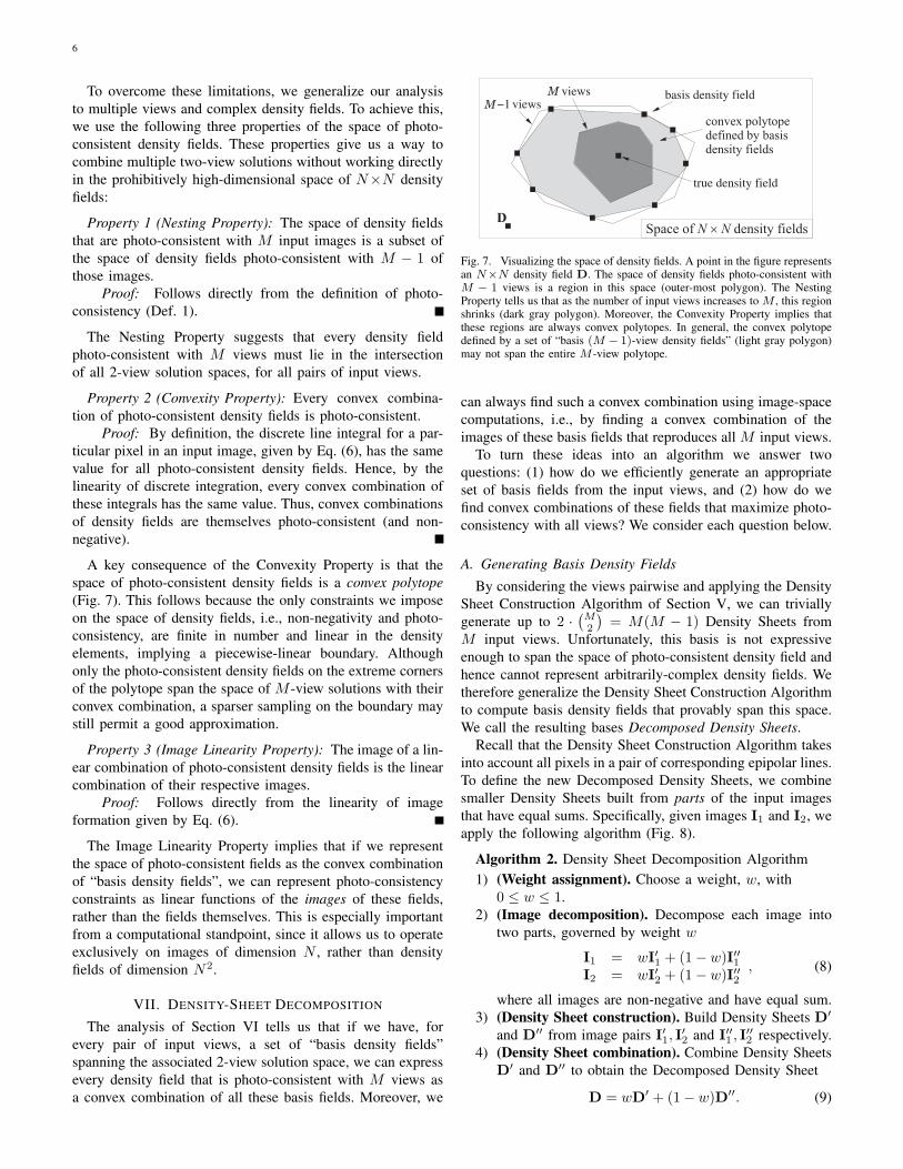
DSpace of density fieldsN N´

convex polytopedefined by basisdensity fields

M

M

Fig. 7. Visualizing the space of density fields. A point in the figure representsan N×N density field D. The space of density fields photo-consistent withM − 1 views is a region in this space (outer-most polygon). The NestingProperty tells us that as the number of input views increases to M , this regionshrinks (dark gray polygon). Moreover, the Convexity Property implies thatthese regions are always convex polytopes. In general, the convex polytopedefined by a set of “basis (M − 1)-view density fields” (light gray polygon)may not span the entire M -view polytope.

can always find such a convex combination using image-space

computations, i.e., by finding a convex combination of the

images of these basis fields that reproduces all M input views.

To turn these ideas into an algorithm we answer two

questions: (1) how do we efficiently generate an appropriate

set of basis fields from the input views, and (2) how do we

find convex combinations of these fields that maximize photo-

consistency with all views? We consider each question below.

A. Generating Basis Density Fields

By considering the views pairwise and applying the Density

Sheet Construction Algorithm of Section V, we can trivially

generate up to 2 ·(

M

2

)

= M(M − 1) Density Sheets from

M input views. Unfortunately, this basis is not expressive

enough to span the space of photo-consistent density field and

hence cannot represent arbitrarily-complex density fields. We

therefore generalize the Density Sheet Construction Algorithm

to compute basis density fields that provably span this space.

We call the resulting bases Decomposed Density Sheets.

Recall that the Density Sheet Construction Algorithm takes

into account all pixels in a pair of corresponding epipolar lines.

To define the new Decomposed Density Sheets, we combine

smaller Density Sheets built from parts of the input images

that have equal sums. Specifically, given images I1 and I2, we

apply the following algorithm (Fig. 8).

Algorithm 2. Density Sheet Decomposition Algorithm

1) (Weight assignment). Choose a weight, w, with

0 ≤ w ≤ 1.

2) (Image decomposition). Decompose each image into

two parts, governed by weight w

I1 = wI′1 + (1 − w)I′′1

I2 = wI′2 + (1 − w)I′′2

, (8)

where all images are non-negative and have equal sum.

3) (Density Sheet construction). Build Density Sheets D′

and D′′ from image pairs I

′1, I

′2 and I

′′1 , I′′2 respectively.

4) (Density Sheet combination). Combine Density Sheets

D′ and D

′′ to obtain the Decomposed Density Sheet

D = wD′ + (1 − w)D′′. (9)

7

D

= +

D

t

t

D

t t

t t

Fig. 8. Decomposing I1 and I2 into component parts according to w. I1 is decomposed into a central interval of pixels, wI′1

, whose fraction of the totalsum is w, and the remainder, (1 − w)I′′

1, whose fraction of the sum is 1 − w. I2 is decomposed analogously, according to w as well. The central intervals

of I1, I2 are offset from the first pixel in the images by t1 and t2 respectively. Also shown are the two Density Sheets with opposite diagonal orientations,D′ and D′′, computed from corresponding pairs of parts (Sec. V).

Note that the resulting Decomposed Density Sheet, D, will

always be photo-consistent with the input images I1, I2. This

is a direct consequence of the Convexity and Image Linearity

Properties of Section VI.To fully specify the algorithm we must describe how to

decompose the images in Step 2, given some choice of the

weight w. To do this, we split I1 and I2 into a central

interval of pixels, whose fraction of the total sum is w, and

the remainder (Fig. 8). The resulting density field therefore

retains the sheet-like structure of the basic Density Sheet in a

piecewise fashion. Note that we construct D′ and D

′′ with

opposite diagonal orientation, otherwise their combination

would simply be one of the Density Sheets for the input

images.The family of Decomposed Density Sheets can thus be

parameterized by the diagonal orientation of D′; the weight of

the central interval w; and the offsets of the central intervals I′1

and I′2 from the first pixel in the images. Therefore, given W

distinct weights and T distinct offsets, we can create 2WT 2

Decomposed Density Sheets using this method.Intuitively, when we are restricted to a limited number of

these bases, we would like to choose them so that central

Density Sheet “covers” all areas of the density field. As we

change the offset parameters, the rectangular region containing

wD′ will translate over the N×N field, motivating a simple

scheme where the T offsets for a central interval of weight

w ≥ 1/T are distributed linearly over the whole range.

Specifically, we define the set of offsets for each input image

as t1, t2 ∈ { iT−1 (1 − w)}T−1

i=0 . By varying the diagonal

orientation of the central Density Sheet and selecting the offset

for each input image, we thus obtain 2T 2 bases for each

choice of the weight. Likewise, we adopt a simple method

to distribute the W different weights linearly, according to

w ∈ { 1T

+ T−1T

kW}W−1

k=0 .

B. Completeness Theorem

A fundamental property of Decomposed Density Sheets

is that even though they are easy to generate, the subspace

they span contains all density fields that are photo-consistent

with the input views. We derive this result by analyzing the

space of photo-consistent density fields and showing that we

can generate enough Decomposed Density Sheets to span this

space. Specifically we know from Section VI that the space

of photo-consistent density fields is a convex polytope. First

we show that this polytope lies in an (N − 1)2-dimensional

hyperplane:

Theorem 2: The space of N ×N density fields that are

photo-consistent with two views is an (N − 1)2-dimensional

convex polytope in the space of N×N matrices.

Proof: See Appendix B for a constructive proof.

Next we show that the Decomposed Density Sheets form a

complete basis for the space of photo-consistent density fields,

by constructing a family of Decomposed Density Sheets that

spans the (N − 1)2-dimensional hyperplane. In other words,

the parameters of the Decomposed Density Sheets (diagonal

orientation, weight, and offsets in the input images) give us

enough degrees of freedom to generate bases that span the

space:

Theorem 3 (Density Sheet Completeness): The family of

Decomposed Density Sheets forms a complete basis for the

space of M -view photo-consistent density fields.

Proof: (Sketch). We first show how to construct a linearly

independent basis of Decomposed Density Sheets for the

special case of density fields that are photo-consistent with

two constant input images, I1 = I2 = α[1 . . . 1]T . We then

derive transformations that let us reduce the general problem

to this case. See Appendix C for a full proof.

C. Decomposed Density Sheet Reconstruction

With the procedure for generating Decomposed Density

Sheets (Sec. VII-A) as a starting point, we rely on the

following algorithm to compute an epipolar slice of the density

field that maximizes photo-consistency with M views:

Algorithm 3. Decomposed Density Sheet Reconstruction

Algorithm

1) (Basis construction). For each of P = M(M − 1)/2pairs of views, generate a family of B Decomposed Den-

sity Sheets, {Dp 1,Dp 2, . . . ,Dp B} using Algorithm 2.

Warp these into a common global coordinate system.

2) (Basis projection). Project the Decomposed Density

Sheets to all input viewpoints, and stack their images

8

into MP blocks, each of size N × B:

Fm p =[

Im(Dp 1) Im(Dp 2) · · · Im(Dp B)]

,

where the notation Im(D) refers to the projection of

density field D to image Im using discrete integration

(Eq. (6)).

3) (QP formation). Stack the blocks from Step 2 and the

input images together,

F =

F1 1 F1 2 · · · F1 P

F2 1 F2 2 · · · F2 P

...

FM 1 FM 2 · · · FM P

, I =

I1

I2

...

IM

,

to form the following quadratic programming problem:

minimize ||Fx − I||2

subject to∑

x = 1,x ≥ 0 .

4) (QP solution). Solve this quadratic optimization prob-

lem by any standard method (e.g., [39]). The resulting

optimal x gives the weights needed to express the den-

sity field as a convex combination of the Decomposed

Density Sheets computed in Step 1.

Because the quadratic programming problem is convex, the

solver will find a global minimum of the objective function.

This solution is not necessarily unique because the minimum

||Fx − I||2 = 0 will be attained by all density fields of this

form that are photo-consistent.

D. Discussion

The result of this algorithm is a reconstruction of the density

field as a superposition of piecewise Density Sheets defined by

pairs of views. These sheets are convex combinations of the

various Decomposed Density Sheet bases. As with the basic

Density Sheet solution, the sheet-like structures are well-suited

to view synthesis because they allow us to effectively warp

pieces of the original images in order to render them.

If the P ·B Decomposed Density Sheets computed by a

run of Algorithm 3 are such that a convex combination is

photo-consistent with all views, the algorithm will attain the

optimal lower bound, ||Fx−I||2 = 0. Otherwise, it will return

the convex combination of bases that minimizes inconsistency

with the input images in a least-squared sense.

Note that Step 3 of the algorithm is suboptimal because

a combination of Decomposed Density Sheets constrained

to be convex may not in general span all M -view photo-

consistent solutions (Fig. 7). While optimizing over linear,

rather than convex, combinations of sufficiently many sheets

would avoid this problem, this would incur a significant

computational cost. This is because explicit enforcement of

non-negativity constraints for arbitrary linear combinations

requires working directly in the N2-dimensional space of

density fields. In practice, we enforce the convex combination

constraint exclusively.

As described in Section IV, this algorithm is applied in-

dependently to a collection of epipolar planes slicing through

the 3D volume. The coherence between adjacent epipolar lines

in the input images, however, implies that adjacent slices of

the volume will have similar decompositions. In practice this

tends to generate a superposition of coherent 2D surfaces in

the 3D volume5.

VIII. EXPERIMENTAL RESULTS

We performed experiments on a variety of scenes of fire,

some simulated and some real. Here we show results from

three scenes containing real fire that try to convey a range of

different flame structures.6 We show that the basic Density

Sheet produces excellent results for simple to moderately

complex flames, and that the Density-Sheet Decomposition

Algorithm is useful for reconstructing more complex scenes

of fire.

A. “Torch” dataset

The first scene (“torch”) was a citronella patio torch, burning

with a flickering flame about 10cm tall. Two synchronized

progressive-scan Sony DXC-9000 cameras, roughly 90◦ apart,

were used to acquire videos of the flame at 640×480 resolution

(Fig. 2). While ground truth for this scene was not available,

the structure of the flame is simple, and it appears that epipolar

slices actually contain a single elongated blob of density.

The cameras were calibrated using Bouguet’s Camera Cal-

ibration Toolbox for Matlab [40] to an accuracy of about 0.5

pixels. The input views were then rectified so that correspond-

ing horizontal scanlines define the epipolar slices. For each of

the 25 frames in the video sequence, each epipolar slice was

reconstructed independently.

We compared three different reconstruction methods with

respect to the quality of synthesized views interpolating be-

tween the two cameras (Fig. 9). First, the multiplication solu-

tion shows typical blurring and doubling artifacts. Interpolated

views of this solution do not contain the same high frequency

content as the input images and suggest that the viewpoints

were “accidentally” aligned so as to hide significant structures

in the scene. Second, an algebraic method based on fitting

Gaussian blobs to the density field [41] over-fits the two

input images and produces a badly mottled appearance for

synthesized views. This confirms that sparse-view tomography

methods are not suitable when the number of viewpoints is

extremely limited. Third, the Density Sheet reconstruction

produces very realistic views that appear indistinguishable in

quality from the input views.

If the viewpoint is varied while time is fixed, the true nature

of the Density Sheet reconstruction as a transparent surface can

be perceived. The addition of temporal dynamics, however,

enhances photo-realism. For simple flames like the “torch”

scene, a two-view reconstruction consisting of a single Density

Sheet serves as a good impostor for the true scene.

To render the Density Sheet solution, we first compute the

geometry of the Density Sheet and then use this sheet to

5Formally, it is easy to show that the function that maps input images toDensity Sheets is smooth. This is why Density Sheets from adjacent scanlineshave similar shape when the intensity variation across these scanlines is small(e.g., Fig. 9, rows 3–4).

6See http://www.cs.toronto.edu/∼hasinoff/fire for color images and videoclips, as well as more results.

9

0◦ (input) 23◦ 45◦ 68◦ 90◦ (input) density field (scanline 275)

mu

ltip

lica

tio

nso

luti

on

blo

b-b

ased

met

ho

d[4

1]

Den

sity

Sh

eet

solu

tio

n

0◦ (input) 23◦ 45◦ 68◦ 90◦ (input)

Den

sity

Sh

eet

geo

met

ry

Fig. 9. Three different reconstructions of the “torch” dataset (frame 8) from two input images. Labels on the left indicate the method used. On the right weshow a top view of a reconstructed epipolar slice, corresponding to the white horizontal line in the 0◦ images (dark regions denote areas with concentratedfire density). Note that the multiplication and Density Sheet solutions reproduce the input images exactly. The bottom row illustrates the 3D geometry of theDensity Sheet solution, rendered as a specular surface.

10

warp the input images to the interpolated view by backward

mapping [24]. We then blend the warped input images accord-

ing to a simple view-dependent linear interpolation. To render

the other solutions, we use standard volume rendering which

applies discrete integration to the reconstructed 3D density

field.

B. “Burner” dataset

The second scene (“burner”), courtesy Ihrke and Magnor

[23], [42], consists of a colorful turbulent flame emanating

from a gas burner. This scene was captured for 348 frames

using eight synchronized video cameras with 320 × 240resolution. The cameras are roughly equidistant from the flame

and distributed over the viewing hemisphere. Ground truth is

not available for this scene either, but an algebraic tomography

method restricted by the visual hull produces a reasonable

approximation to the true density field [23].

For the “burner” dataset we applied our algorithms to

just two of the input cameras, spaced about 60◦ apart. We

used the calibration provided to rectify the images from this

pair of cameras and then computed the Density Sheet from

corresponding scanlines. Finally, as in view morphing [43],

we used a homography to warp the images synthesized in the

rectified space back to the interpolated camera (Fig. 10).

Although the “burner” scene is significantly more complex

than the previous scene, two-view reconstruction using a single

Density Sheet can still produce realistic intermediate views

(Fig. 10, rows 1–2). As with the “torch” dataset, the view

interpolation appears even more plausible when the dynamics

of the flame are added.

As shown in the third row of Fig. 10, a significant artifact

occurs when the true flame consists of multiple structures and

when our imaging model (Sec. III) is not satisfied exactly. In

this example, the true scene and both input images consist

of two major flame structures, but the images disagree on

the total intensity (i.e., the total density) of each structure.

For the Density Sheet solution, this discrepancy leads to a

“tearing” effect where a spurious thin vertical structure is

used to account for the lack of correspondence. Note that this

problem applies more generally to any technique assuming a

linear image formation model for this particular dataset.

We also compare interpolated views generated using the

Density Sheet reconstruction and the algebraic tomography

method of Ihrke and Magnor [23]. While the tomography

method uses all 8 cameras to reconstruct a coarse 963 voxel

grid, the Density Sheet reconstruction explains the density field

locally using a single transparent surface defined by the closest

2 cameras. Despite this imbalance, the simple Density Sheet

reconstruction (Fig. 10, bottom) may still be preferable for

view synthesis. The volume renderings produced by algebraic

tomography are relatively noisier, lower resolution, and less

“similar” to the sharp and smooth input images.

C. “Jet” dataset

The third scene (“jet”) consists of a complex flame emerging

from a gaseous jet (Fig. 11, first row). The dataset consists

of 47 synchronized views, roughly corresponding to inward-

facing views arranged around a quarter-circle, captured from a

promotional video for a commercial 3D freeze-frame system

[44]. Since no explicit calibration was available for this

sequence, we assumed that the views were evenly spaced.

To test the view synthesis capabilities of our approach, we

used a subset of the 47 frames as input and used the rest

to evaluate agreement with the synthesized views (Fig. 11).

Rendering results from the multiplication solution and the

Density Sheet solution (Algorithm 1) suggest that these so-

lutions cannot accurately capture the flame’s appearance and

structure, and are not well suited to more complex flames with

large appearance variation across viewpoint. To incorporate

more views, we applied the blob-based algebraic tomography

method in [41] and the Density Sheet Decomposition Algo-

rithm (Algorithm 3) with the 45◦ view as a third image. In the

latter algorithm, we generated B = 150 Decomposed Density

Sheets for each of the P = 3 pairs of input views in Step 1,

giving rise to a total of 450 basis density fields.

To further explore the benefit of using multiple views, we

optimized the convex combination of these fields in Steps 2-4

in two ways: (1) by maximizing photo-consistency with the

three input images and (2) by maximizing photo-consistency

with four additional images from the sequence, but using the

same three-view basis7. The results in Fig. 11 and Table I

suggest that the Density Sheet Decomposition Algorithm pro-

duces rendered images that are superior to the other methods.

They also show that increasing the number of images has a

clear benefit.

Three observations can be made from these experiments.

First, the convex combination of Decomposed Density Sheets

can capture the structure of complex flames because the sheets

sweep out regions of the density field, explaining fire density

at multiple depths. Second, the resulting algorithm can render

complex flames from a small number of input views, without

the doubling artifacts of the multiplication solution or the

over-fitting artifacts of the blob-based method. This is because

the family of Decomposed Density Sheets is expressive and

induces a bias toward compact solutions. Third, the sheets’

surface-like structure enables photo-realistic rendering of com-

plex semi-transparent scenes by simply warping and blending

partial input images (Eq. (8)). Thus, the density models we

extract may be suitable for interactive graphics applications.

IX. DISCUSSION

One feature of semi-transparency is that no part of the scene

will be occluded as long as the camera exposure is set to

prevent saturation. This benefit, however, comes at the cost that

the space of photo-consistent density fields is fundamentally

ambiguous when the number of input views is small. In this

work, we have assumed spatial coherence in the density field

in order to achieve good view synthesis.

7The reason for using M ′ > M views for photo-consistency and M forbasis computation is that this leaves unchanged the number of unknownsin the quadratic programming problem. With a constant number of bases perview-pair (Sec. VII-A), the number of unknowns grows according to O(M2),not O(M ′2), which makes the problem less computationally intensive.

11

input (camera 3) —————————— reconstructed views —————————— input (camera 4)

fram

e3

17

fram

e2

71

fram

e1

39

Density Sheet algebraic tomography Density Sheet algebraic tomography(cameras 3 and 4) (cameras 1–8) (cameras 3 and 4) (cameras 1–8)

fram

e1

87

fram

e1

91

Fig. 10. Density Sheet reconstruction of the “burner” dataset [23], [42], interpolating between two cameras about 60◦ apart. At top, the first and lastcolumns are input views; the middle columns are interpolated. Each row represents a different frame from the turbulent flame sequence. The highlightedregion draws attention to a spurious thin structure present in interpolated views of the third row. This artifact is due to inexact correspondence between majorflame structures because our imaging model is violated. At bottom, we compare views interpolated using the Density Sheet, midway between the two cameras,alongside nearby views generated by an algebraic tomography method using all 8 cameras [23].

12

45◦ (input) 68◦ inset 0◦ (input) 90◦ (input)

gro

un

dtr

uth

45◦ 68◦ inset 135◦ density field

mu

ltip

lica

tio

n(2

)d

ensi

tysh

eet

(2)

blo

bs

(3)

dec

om

po

siti

on

(3)

dec

om

po

siti

on

(3+

4)

Fig. 11. Reconstruction of the “jet” dataset. Ground truth images of the fire are shown in the top row; the remaining rows correspond to different reconstructionmethods. Labels on the left indicate the method used, with the number of input views in brackets. From left to right: 45◦ view, which is synthesized for themultiplication and Density Sheet solutions and is an input view for the other methods; 68◦ view, synthesized for all methods; zoomed-in view of the regionmarked in the 68◦ image; 135◦ view, which is a distant extrapolation; and top view of a reconstructed epipolar slice, corresponding to the white horizontalline in the 135◦ image (dark regions denote areas with concentrated fire density).

13

TABLE I

PER-PIXEL RMS RECONSTRUCTION ERROR FOR THE “JET” DATASET.

reconstruction method (views)RMS error

input all

density sheet solution (2)a 0 26.6multiplication solution (2) 0 21.5blob-based method [41] (3) 13.3 19.0density sheet decomposition (3) 10.1 18.4

density sheet decomposition (3+4)b 11.5 15.8

aThe first two reconstructions reproduce the input views exactly.bThree input views were used to generate the basis, and four additional

views were used to evaluate photo-consistency only.

It would be useful to understand how photo-consistency

constraints from three or more views restrict the space of two-

view and M -view solutions. In particular, a third view would

be expected to eliminate much of the ambiguity that causes

the doubling of sharp features found in the multiplication

solution (Fig. 4). Such a view is less likely to be helpful

for disambiguating smooth and diffuse regions because, as

in standard stereo, the lack of high-frequency detail makes

unambiguous reconstruction in these regions more difficult.

So far we have assumed that the cameras are restricted to

lie on the same plane, but most previous methods for semi-

transparent reconstruction extend readily to general viewing

configurations (at least in theory). Unfortunately, in such

configurations the basis coefficients from different 2D slices

of the 3D density field become linked, leading to much larger

quadratic programming problems. In the worst case, with three

orthogonal views, the coefficients of all Decomposed Density

Sheet bases from all slices are needed to evaluate photo-

consistency for a single pixel. To enhance computational effi-

ciency, it might be possible to consider Decomposed Density

Sheet bases defined in 3D and construct from bands of epipolar

lines in the input views.

From the point of view of fire reconstruction, simultaneous

recovery of the 3D temperature, density, and pressure fields,

commonly used in combustion engineering and computer

graphics [1], [11] appears to be a daunting task. Consequently,

simpler models of fire, like the one we describe in Section III,

dominate current reconstruction techniques. This suits our

purpose, since we are more interested in modeling appearance

variation than extracting particular physical properties of fire.

In fact, the advantage of any image-based technique is that any

flames we can observe can be reconstructed directly, without

modeling or simulating their interaction with the environment

[1], [6].

X. CONCLUDING REMARKS

In this article we introduced Density Sheets as a basic

primitive for representing, reconstructing, and rendering semi-

transparent scenes from a small number of input views. This

primitive was derived through a detailed analysis of the space

of densities that are photo-consistent with two or more views

and was designed with four key properties in mind—photo-

consistency, uniqueness, spatial compactness, and representa-

tional completeness. We showed that these properties lead to

simple reconstruction algorithms that produce stable solutions

even for very limited numbers of input views (even two),

despite the ill-posed nature of the volumetric reconstruction

problem. Importantly, we showed that the behavior and solu-

tion space of these algorithms can be characterized and that

the resulting reconstructions have good view interpolation and

extrapolation capabilities.

The question of how best to capture the global 3D struc-

ture and dynamics of fire and other physical phenomena

remains open. Toward this goal, we are investigating new

spatio-temporal coherence constraints and ways to integrate

our approach with traditional simulation methods. In theory,

image-based reconstructions could be used to train or validate

physical simulators, and these simulators could be used to

evaluate reconstructions in terms of their physical plausibility.

While our experiments suggest that Density Sheets and the

Density-Sheet Decomposition Algorithm are useful for fire

reconstruction, these tools may also prove useful in more

general contexts. This includes the reconstruction of other

volumetric phenomena such as smoke [4], sparse-view tomog-

raphy problems in medical diagnostics [20], and accelerated

image-based methods for volume rendering.

APPENDIX A

PROOF OF THEOREM 1

Proof: (By induction) We show that Algorithm 1 gen-

erates a density field D with the desired properties. The

downward and rightward expansions in Step 3 guarantee that

the elements of D traced by the pair (r, c) define a monotonic

four-connected curve. Therefore it is sufficient to show that

D is non-negative and photo-consistent. For ease of notation,

we denote the row and column sums of D by s1 = D1 and

s2 = DT1 respectively, where 1 = [1 . . . 1]T .

We show that properties H1–H4, corresponding to our

induction hypothesis, hold throughout the course of the algo-

rithm, as the element (r, c) traces a path from (1, 1) to (N,N):

H1: D is photo-consistent with the sub-vectors

I1(1, . . . , r − 1) and I2(1, . . . , c − 1);H2: D is photo-consistent with I1(r) or I2(c);H3: D satisfies s1 ≤ I1 and s2 ≤ I2; andH4: D ≥ 0.

For the base case (r, c) = (1, 1), H1–H4 are trivially satisfied

after Step 2 of the algorithm.

Part I: The algorithm terminates with D photo-consistent

with I1, I2. First we show that if D is photo-consistent with

one of the vectors I1, I2 then H1–H4 imply that D must be

photo-consistent with both of them. In particular, assume wlog

that (r, c) = (N, j) and s1 = I1. From H3 we know that

s2(j) ≤ I2(j), and because∑

I1 =∑

I2, all density must be

distributed within the first j columns. Thus I2(j+1, . . . , N) =0 and s2(j) = I2(j), implying that I2 is photo-consistent as

well. Second, we note that the expansions prescribed by Step 3

of the algorithm are valid even at the boundary cases: if r = Nthen the expansion will be rightward; if c = N , the expansion

will be downward unless s1(r) < I1(r). But this inequality is

never satisfied: if s1(r) < I1(r), H2–H3 imply that s2 = I2

and therefore s1 = I1, leading to a contradiction. Thus, the

algorithm always terminates with (r, c) = (N,N).

14

+1

i

j

Sij =

+1 -1

-1N

N

0

Fig. 12. The matrices {Sij}i,j<N , form a basis for the space of N×Nphoto-consistent matrices. Each matrix contains only four non-zero elementsarranged in a rectangle whose bottom-right corner is fixed at element (N, N).Sij is zero in the gray-shaded regions. Clearly, Sij 1 = 0 and ST

ij 1 = 0.

Part II: Every application of Step 3 preserves the induction

hypothesis. If the expansion is rightward then either s1(r) <I1(r) or s1 = I1. In the first case, H2–H3 imply that s2(c) =I2(c). Then, by construction, D(r, c + 1) will be set to some

non-negative value so that either the new column is photo-

consistent (i.e., s2(c + 1) = I2(c + 1)), or the current row

becomes photo-consistent (i.e., s1(r) = I1(r)). Both outcomes

preserve H1–H4 for (r, c + 1). If s1 = I1, it must also be the

case that s2 = I2 and setting D(r, c) = 0 as prescribed by

Step 3 of the algorithm preserves H1–H4. Analogously, every

downward expansion also preserves the inductive hypothesis.

Therefore the algorithm terminates with (r, c) = (N,N)and H1–H4 intact. Hence, D ≥ 0 and D is photo-consistent

with both vectors. The proof for D′ is analogous.

APPENDIX B

PROOF OF THEOREM 2

Proof: From Section VI, we know that the space of

photo-consistent density fields is a convex polytope. We show

that it is (N − 1)2-dimensional in the two-view case.

Given two non-negative, N -dimensional column vectors I1

and I2, consider an N×N matrix D whose row and column

sums, respectively, are equal to these vectors, i.e., D1 = I1

and DT1 = I2. Every such matrix can be expressed as

D = D0 + S, where D0 is any photo-consistent density (e.g.,

the multiplication solution), and S preserves row and column

sums, i.e., S1 = 0 and ST1 = 0. Note that fixing the

(N − 1)× (N − 1) upper-left block of S uniquely defines the

remaining elements, giving us an upper bound of (N −1)2 on

the dimensionality of the polytope.

We now show that the (N − 1)2 upper bound is tight by

explicitly constructing a basis for the polytope’s hyperplane

that consists of (N − 1)2 linearly-independent matrices. In

particular, consider the family of N×N matrices {Sij}i,j<N

defined in Fig. 12, where each matrix consists of four non-zero

elements arranged in a rectangle. Adding a matrix Sij to D0

has the effect of shifting mass from two diagonal corners of the

rectangle to the other two corners.8 The matrices {Sij}i,j<N

are linearly independent since Sij(i, j) = 1 and Si′j′(i, j) = 0for all other i′, j′ < N . Therefore they span the (N − 1)2-

dimensional hyperplane.

8The matrices Sij can be thought of a generalization to continuous-valueddensity fields of the “switching matrices” described in [27].

The hyperplane can be expressed as a linear combination

of the resulting two-view photo-consistent matrices, D0 and

{D0 + Sij}i,j<N .

APPENDIX C

PROOF OF THEOREM 3

Lemma 1: Let Σc be the set of non-negative N×N matrices

whose row and column sums are constant vectors, i.e., Σc ={D |D1 = α1 and D

T1 = α1} for some α ∈ R. The

Decomposed Density Sheets form a basis spanning Σc.

Proof: Assume wlog that α = 1. Theorem 2 tells us

that the set Σc is an (N − 1)2-dimensional polytope. We use

a constructive proof, specifying Decomposed Density Sheet

matrices that span this polytope’s hyperplane.

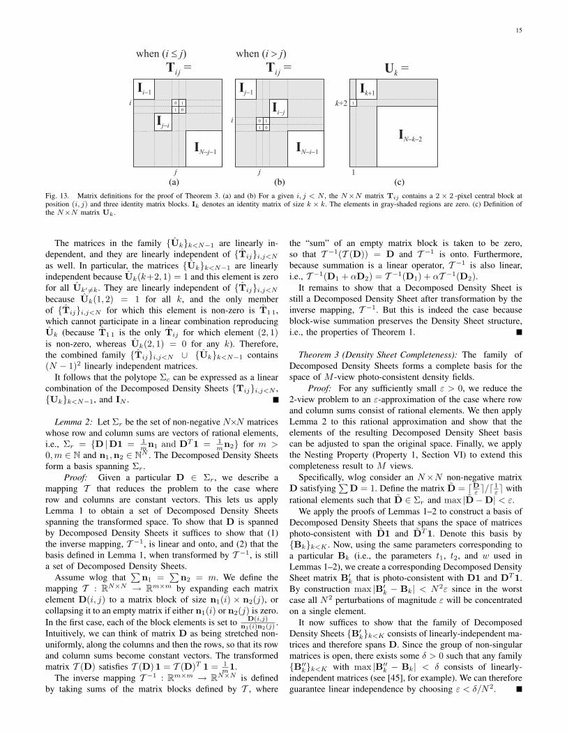
First consider the family of N × N binary matrices

{Tij}i,j<N defined in Fig. 13a,b. These matrices are zero

except for three identity-matrix blocks and a 2 × 2 block

at position (i, j). Each matrix Tij satisfies Tij 1 = 1 and

TTij 1 = 1 and therefore belongs to Σc. Moreover, Tij is

a Decomposed Density Sheet corresponding to the output of

Algorithm 2 with I1 = I2 = 1 and specified by the parameters

t1 = i−1N

, t2 = j−1N

, and w = 2N

(see Sec. VII-A).

We now define matrix Tij = Tij − IN and show that the

family {Tij}i,j<N is linearly independent for i 6= j + 1. This

provides us with a basis of dimension (N−1)2−(N−2), each

of whose members, Tij , is the difference of two Decomposed

Density Sheets (IN and Tij). Note that each Tij will have

elements with values 1, 0 or -1. Furthermore, note the recursive

structure of {Tij}, where the upper-leftmost (N−1)×(N−1)block of a given Tij with i, j < N − 1 corresponds directly

to matrix Tij for a problem of size N − 1.

We use induction on N to obtain our linear independence

result, where the induction hypothesis for N − 1 implies that

{Tij}i,j<N−1 are linearly independent for i 6= j+1. The base

cases for N ≤ 2 are trivial. Given the induction hypothesis,

it remains to show that the addition of the 2N − 4 matrices,

{TN−1, j}j<N−2 and {Ti, N−1}i<N , preserves linear inde-

pendence. This is simple to show, since TN−1, j(N, j) = 1for j < N−2, but the element (N, j) is zero for all other Tij .

Similarly, Ti, N−1(i,N) = 1 for i < N , but apart from the

case i = N − 2, the element (i,N) is zero for all other Tij .

This leaves just TN−2, N−1, for which element (N − 2, N)is non-zero in {TN−1, j}j<N−2 as well. However, none of

these other matrices can participate in a linear combination

reproducing TN−2, N−1, since they comprise the only Tij for

which any of the elements {(N, k)}N−3k=1 are non-zero.

The family {Tij}i,j<N gives us (N − 1)2 − (N − 2)linearly independent matrices. So to obtain a basis for the

(N−1)2 dimensions of Σc we need N−2 additional linearly-

independent matrices. To construct them, we consider a second

family of N × N matrices {Uk}k<N−1, shown in Fig. 13c.

This family contains a total of N −2 members, each of which

belongs to Σc. Moreover, Uk is a Decomposed Density Sheet

by construction, corresponding to the output of Algorithm 2

with I1 = I2 = 1 and parameters t1 = k+1N

, t2 = 0, and

w = 12N

. Similarly, define Uk = Uk − IN .

15

1

1

Ij 1-

IN i 1- -

Ii j-

i

j

0

0

when ( )i j>

1

1

Ii 1-

IN j 1- -

Ij i-

i

j

0

0

Ti j =when ( )i j£

1

Ik+1

IN k- 2-

k+2

1

Uk =Ti j =

(a) (b) (c)

Fig. 13. Matrix definitions for the proof of Theorem 3. (a) and (b) For a given i, j < N , the N×N matrix Tij contains a 2 × 2 -pixel central block atposition (i, j) and three identity matrix blocks. Ik denotes an identity matrix of size k × k. The elements in gray-shaded regions are zero. (c) Definition ofthe N×N matrix Uk .

The matrices in the family {Uk}k<N−1 are linearly in-

dependent, and they are linearly independent of {Tij}i,j<N

as well. In particular, the matrices {Uk}k<N−1 are linearly

independent because Uk(k+2, 1) = 1 and this element is zero

for all Uk′ 6=k. They are linearly independent of {Tij}i,j<N

because Uk(1, 2) = 1 for all k, and the only member

of {Tij}i,j<N for which this element is non-zero is T1 1,

which cannot participate in a linear combination reproducing

Uk (because T1 1 is the only Tij for which element (2, 1)is non-zero, whereas Uk(2, 1) = 0 for any k). Therefore,

the combined family {Tij}i,j<N ∪ {Uk}k<N−1 contains

(N − 1)2 linearly independent matrices.

It follows that the polytope Σc can be expressed as a linear

combination of the Decomposed Density Sheets {Tij}i,j<N ,

{Uk}k<N−1, and IN .

Lemma 2: Let Σr be the set of non-negative N×N matrices

whose row and column sums are vectors of rational elements,

i.e., Σr = {D |D1 = 1m

n1 and DT1 = 1

mn2} for m >

0,m ∈ N and n1,n2 ∈ NN . The Decomposed Density Sheets

form a basis spanning Σr.

Proof: Given a particular D ∈ Σr, we describe a

mapping T that reduces the problem to the case where

row and columns are constant vectors. This lets us apply

Lemma 1 to obtain a set of Decomposed Density Sheets

spanning the transformed space. To show that D is spanned

by Decomposed Density Sheets it suffices to show that (1)

the inverse mapping, T −1, is linear and onto, and (2) that the

basis defined in Lemma 1, when transformed by T −1, is still

a set of Decomposed Density Sheets.

Assume wlog that∑

n1 =∑

n2 = m. We define the

mapping T : RN×N → R

m×m by expanding each matrix

element D(i, j) to a matrix block of size n1(i) × n2(j), or

collapsing it to an empty matrix if either n1(i) or n2(j) is zero.

In the first case, each of the block elements is set toD(i,j)

n1(i)n2(j).

Intuitively, we can think of matrix D as being stretched non-

uniformly, along the columns and then the rows, so that its row

and column sums become constant vectors. The transformed

matrix T (D) satisfies T (D)1 = T (D)T1 = 1

m1.

The inverse mapping T −1 : Rm×m → R

N×N is defined

by taking sums of the matrix blocks defined by T , where

the “sum” of an empty matrix block is taken to be zero,

so that T −1(T (D)) = D and T −1 is onto. Furthermore,

because summation is a linear operator, T −1 is also linear,

i.e., T −1(D1 + αD2) = T −1(D1) + αT −1(D2).It remains to show that a Decomposed Density Sheet is

still a Decomposed Density Sheet after transformation by the

inverse mapping, T −1. But this is indeed the case because

block-wise summation preserves the Density Sheet structure,

i.e., the properties of Theorem 1.

Theorem 3 (Density Sheet Completeness): The family of

Decomposed Density Sheets forms a complete basis for the

space of M -view photo-consistent density fields.

Proof: For any sufficiently small ε > 0, we reduce the

2-view problem to an ε-approximation of the case where row

and column sums consist of rational elements. We then apply

Lemma 2 to this rational approximation and show that the

elements of the resulting Decomposed Density Sheet basis

can be adjusted to span the original space. Finally, we apply

the Nesting Property (Property 1, Section VI) to extend this

completeness result to M views.

Specifically, wlog consider an N×N non-negative matrix

D satisfying∑

D = 1. Define the matrix D = ⌈D

ε⌉/⌈ 1

ε⌉ with

rational elements such that D ∈ Σr and max |D − D| < ε.

We apply the proofs of Lemmas 1–2 to construct a basis of

Decomposed Density Sheets that spans the space of matrices

photo-consistent with D1 and DT1. Denote this basis by

{Bk}k<K . Now, using the same parameters corresponding to

a particular Bk (i.e., the parameters t1, t2, and w used in

Lemmas 1–2), we create a corresponding Decomposed Density

Sheet matrix B′k that is photo-consistent with D1 and D

T1.

By construction max |B′k − Bk| < N2ε since in the worst

case all N2 perturbations of magnitude ε will be concentrated

on a single element.

It now suffices to show that the family of Decomposed

Density Sheets {B′k}k<K consists of linearly-independent ma-

trices and therefore spans D. Since the group of non-singular

matrices is open, there exists some δ > 0 such that any family

{B′′k}k<K with max |B′′

k − Bk| < δ consists of linearly-

independent matrices (see [45], for example). We can therefore

guarantee linear independence by choosing ε < δ/N2.

16

REFERENCES

[1] D. Nguyen, R. Fedkiw, and H. Jensen, “Physically based modeling andanimation of fire,” in Proc. ACM SIGGRAPH, 2002, pp. 721–728.

[2] J. Stam and E. Fiume, “Depicting fire and other gaseous phenomenausing diffusion processes,” in Proc. ACM SIGGRAPH, 1995, pp. 129–136.

[3] R. Fedkiw, J. Stam, and H. W. Jensen, “Visual simulation of smoke,” inProc. ACM SIGGRAPH, 2001, pp. 15–22.

[4] T. Hawkins, P. Einarsson, and P. Debevec, “Acquisition of time-varyingparticipating media,” in Proc. ACM SIGGRAPH, 2005, pp. 812–815.

[5] N. Foster and D. N. Metaxas, “Modeling the motion of a hot, turbulentgas,” in Proc. ACM SIGGRAPH, 1997, pp. 181–188.

[6] A. Lamorlette and N. Foster, “Structural modeling of flames for aproduction environment,” in Proc. ACM SIGGRAPH, 2002, pp. 729–735.

[7] N. Chiba, K. Muraoka, H. Takahashi, and M. Miura, “Two-dimensionalvisual simulation of flames, smoke and the spread of fire,” J. Visualiz.

and Comp. Anim., vol. 5, no. 1, pp. 37–54, Jan.–Mar. 1994.[8] Y. Takai, K. Ecchu, and N. K. Takai, “A cellular automaton model of

particle motions and its applications,” The Visual Computer, vol. 11,no. 5, pp. 240–252, 1995.

[9] R. T. Baum, K. B. McGrattan, and M. Nyden, “An examination ofthe applicability of computed tomography for the measurement ofcomponent concentrations in fire-generated plumes,” Combustion and

Flame, vol. 113, pp. 358–372, 1998.[10] D. P. Correia, P. Ferrao, and A. Caldeira-Pires, “Advanced 3D emis-

sion tomography flame temperature sensor,” Combustion Science and

Technology, vol. 163, pp. 1–24, 2001.[11] A. Schwarz, “Multi-tomographic flame analysis with a schlieren appa-

ratus,” Measurement Science & Tech., vol. 7, pp. 406–413, 1996.[12] W. Xue, W. Donglou, and P. Gongpei, “Use of Moire tomography

to measure the temperature field of the flame of a pyrotechnicalcomposition from its infrared radiation,” Combustion, Explosion, and

Shock Waves, vol. 37, no. 4, pp. 440–442, 2001.[13] G. W. Faris and R. L. Byer, “Beam-deflection optical tomography,”

Optics Letters, vol. 12, no. 3, pp. 72–74, 1987.[14] A. K. Agrawal, N. Butuk, S. R. Gollahalli, and D. Griffin, “Three-

dimensional rainbow schlieren tomography of a temperature field in gasflows,” Applied Optics, vol. 37, no. 3, pp. 479–485, 1998.

[15] B. W. Albers and A. K. Agrawal, “Schlieren analysis of an oscillatinggas-jet diffusion flame,” Combustion and Flame, vol. 199, pp. 84–94,1999.

[16] T. Otsuka and P. Wolanski, “Particle image velocimetry (PIV) analysisof flame structure,” Journal of Loss Prevention in the Process Industries,vol. 14, no. 6, pp. 503–507, 2001.

[17] A. Schodl, R. Szeliski, D. H. Salesin, and I. Essa, “Video textures,” inProc. ACM SIGGRAPH, 2000, pp. 489–498.

[18] D. Drysdale, An Introduction to Fire Dynamics, 2nd ed. Chichester:John Wiley and Sons, 1998.

[19] P. J. Narayanan, P. W. Rander, and T. Kanade, “Constructing virtualworlds using dense stereo,” in Proc. Int’l Conf. on Computer Vision,1998, pp. 3–10.

[20] A. C. Kak and M. Slaney, Principles of Computerized Tomographic

Imaging. New York: IEEE Press, 1988.[21] T. Frese, C. A. Bouman, and K. Sauer, “Adaptive wavelet graph model

for Bayesian tomographic reconstruction,” IEEE Transactions on Image

Processing, vol. 11, no. 7, pp. 756–770, July 2002.[22] R. Szeliski and P. Golland, “Stereo matching with transparency and

matting,” in Proc. Int’l Conf. on Computer Vision, 1998, pp. 517–524.[23] I. Ihrke and M. Magnor, “Image-based tomographic reconstruction

of flames,” in Proc. ACM SIGGRAPH/Eurographics Symposium on

Computer Animation, 2004, pp. 367–375.[24] G. Wolberg, Digital Image Warping. Los Alamitos, CA: IEEE

Computer Society Press, 1990.[25] A. Mohammad-Djafari, “Image reconstruction of a compact object from

a few number of projections,” in Proc. International Conference on

Signal and Image Processing, 1996, pp. 325–329.[26] V. Elangovan and R. T. Whittaker, “From sinograms to surfaces: A direct

approach to the segmentation of tomographic data,” in Proc. Int. Conf.

on Med. Image Computing and Computer-Assisted Intervention, 2001,pp. 213–223.

[27] G. T. Herman and A. Kuba, Eds., Discrete Tomography: Foundations,

Algorithms, and Applications. Boston: Birkhauser, 1999.[28] F. Dachille IX, K. Mueller, and A. Kaufman, “Volumetric backprojec-

tion,” in Proc. IEEE Symp. on Volume Visualization, 2000, pp. 109–117.

[29] J. D. Bonet and P. Viola, “Roxels: Responsibility weighted 3D volumereconstruction,” in Proc. Int’l Conf. on Computer Vision, 1999, pp. 418–425.

[30] R. Bhotika, D. J. Fleet, and K. N. Kutulakos, “A probabilistic theoryof occupancy and emptiness,” in Proc. European Conf. on Computer

Vision, vol. 3, 2002, pp. 112–132.[31] A. Reche, I. Martin, and G. Drettakis, “Volumetric reconstruction

and interactive rendering of trees from photographs,” in Proc. ACM

SIGGRAPH, 2004, pp. 720–727.[32] G. W. Faris and R. L. Byer, “Beam-deflection optical tomography of a

flame,” Optics Letters, vol. 12, no. 3, pp. 155–157, 1987.[33] V. Kwatra, A. Schodl, I. Essa, G. Turk, and A. Bobick, “Graphcut

textures: image and video synthesis using graph cuts,” in Proc. ACM

SIGGRAPH, 2003, pp. 277–286.[34] S. Soatto, G. Doretto, and Y. Wu, “Dynamic textures,” in Proc. Int’l

Conf. on Computer Vision, 2001, pp. 439–446.[35] G. Doretto and S. Soatto, “Editable dynamic textures,” in Proc. Com-

puter Vision and Pattern Recognition, vol. 2, 2003, pp. 137–142.[36] K. Bhat, S. Seitz, J. Hodgins, and P. Khosala, “Flow-based video

synthesis and editing,” in Proc. ACM SIGGRAPH, 2004, pp. 360–363.[37] J. Duderstadt and W. Martin, Transport Theory. New York, NY: John

Wiley and Sons, 1979.[38] C. Silva and J. Santos-Victor, “Intrinsic images for dense stereo matching

with occlusions,” in Proc. European Conf. on Computer Vision, vol. 1,2000, pp. 100–114.

[39] J. Nocedal and S. J. Wright, Numerical Optimization. Springer, 1999.[40] J.-Y. Bouguet, Camera Calibration Toolbox for Matlab (06-Sep-2002).

http://www.vision.caltech.edu/bouguetj/calib doc/.[41] S. Hasinoff, “Three-dimensional reconstruction of fire from images,”

Master’s thesis, University of Toronto, Dept. of Computer Science, 2002.[42] I. Ihrke and M. Magnor, GrOVis-Fire: A multi-video sequence for

volumetric reconstruction and rendering research. http://www.mpi-sb.mpg.de/∼ihrke/Projects/Fire/GrOVis Fire/.

[43] S. Seitz and C. Dyer, “View morphing,” in Proc. ACM SIGGRAPH,1996, pp. 21–30.

[44] Digital Air Incorporated, http://www.virtualcamera.com.[45] G. W. Stewart, Introduction to Matrix Computations. New York:

Academic Press, 1973.

Samuel W. Hasinoff received the BS degree incomputer science from the University of BritishColumbia in 2000, and the MS degree in computerscience from the University of Toronto in 2002.He is currently a PhD candidate at the Universityof Toronto. His research interests include computervision and computer graphics, with a focus on three-dimensional reconstruction, image-based rendering,and computational photography. In 2006, he receivedan honorable mention for the Longuet-Higgins BestPaper Award at the European Conference on Com-

puter Vision. He is a student member of the IEEE.

Kiriakos N. Kutulakos received the BA degree incomputer science at the University of Crete, Greecein 1988, and the MS and PhD degrees in computerscience from the University of Wisconsin, Madisonin 1990 and 1994, respectively. Following his disser-tation work, he joined the University of Rochesterwhere he was an NSF Postdoctoral Fellow and lateran assistant professor until 2001. He is currentlyan associate professor of computer science at theUniversity of Toronto. He won the Best StudentPaper Award at CVPR’94, the Marr Prize in 1999,

a Marr Prize Honorable Mention in 2005 and a Best Paper HonorableMention at ECCV’06. He is the recipient of a CAREER award from the USNational Science Foundation, a Premier’s Research Excellence Award fromthe government of Ontario, and an Alfred P. Sloan Research Fellowship. Heserved as program co-chair of CVPR 2003 and is currently an associate editorof the IEEE Transactions on Pattern Analysis and Machine Intelligence. Heis a member of the IEEE.