PhD Thesis ”Flatness-based Constrained Control

and Model-Free Control Applications to

Quadrotors and Cloud Computing”

Chapter 2: Constraints on Nonlinear Finite

Dimensional Flat Systems

Author: Maria Bekcheva

July 2019

PhD directors: Hugues Mounier and Luca GrecoUniversite Paris-Saclay

This is the second chapter in my thesis ”Flatness-based Constrained Controland Model-Free Control Applications to Quadrotors and Cloud Computing”.Comments and suggestions are most welcome 1.

1maria.bekcheva@l2s.centralesupelec.fr or maria.bekcheva@gmail.com.

1

arX

iv:2

011.

0577

5v1

[ee

ss.S

Y]

11

Nov

202

0

Contents

1 Chapter overview 41.1 Motivation . . . . . . . . . . . . . . . . . . . . . . . . . . . . . . 41.2 Research objective and contribution . . . . . . . . . . . . . . . . 51.3 Existing Methods . . . . . . . . . . . . . . . . . . . . . . . . . . . 71.4 Outline . . . . . . . . . . . . . . . . . . . . . . . . . . . . . . . . 7

2 Differential flatness overview 8

3 Problem statement: Trajectory constraints fulfilment 93.1 General problem formulation . . . . . . . . . . . . . . . . . . . . 93.2 Constraints in the flat output space . . . . . . . . . . . . . . . . 103.3 Problem specialisation . . . . . . . . . . . . . . . . . . . . . . . . 113.4 Closed-loop trajectory tracking . . . . . . . . . . . . . . . . . . . 13

4 Preliminaries on Symbolic Bezier trajectory 144.1 Definition of the Bezier curve . . . . . . . . . . . . . . . . . . . . 154.2 Bezier properties . . . . . . . . . . . . . . . . . . . . . . . . . . . 154.3 Quantitative envelopes for the Bezier curve . . . . . . . . . . . . 174.4 Symbolic Bezier operations . . . . . . . . . . . . . . . . . . . . . 184.5 Bezier time derivatives . . . . . . . . . . . . . . . . . . . . . . . . 19

5 Constrained feedforward trajectory procedure 23

6 Feasible control points regions 246.1 Cylindrical Algebraic Decomposition . . . . . . . . . . . . . . . . 266.2 Approximations of Semialgebraic Sets . . . . . . . . . . . . . . . 27

7 Applications 297.1 Longitudinal dynamics of a vehicle . . . . . . . . . . . . . . . . . 29

7.1.1 Symbolic input constraints . . . . . . . . . . . . . . . . . 307.1.2 Simulation results . . . . . . . . . . . . . . . . . . . . . . 32

7.2 Quadrotor dynamics . . . . . . . . . . . . . . . . . . . . . . . . . 337.2.1 Motivation . . . . . . . . . . . . . . . . . . . . . . . . . . 337.2.2 Simplified model of quadrotor . . . . . . . . . . . . . . . . 357.2.3 Differential flatness of the quadrotor . . . . . . . . . . . . 357.2.4 Constraints . . . . . . . . . . . . . . . . . . . . . . . . . . 367.2.5 Constrained open-loop trajectory u1r . . . . . . . . . . . . 377.2.6 Constrained open-loop trajectories θr et φr . . . . . . . . 387.2.7 Constrained open-loop trajectories xr and yr . . . . . . . 427.2.8 Constrained open-loop trajectories u2 and u3 . . . . . . . 437.2.9 Constrained open-loop control for u4r . . . . . . . . . . . 43

8 Closing remarks 44

A Geometrical signification of the Bezier operations 46

2

B Trajectory Continuity 46

3

Abstract: This chapter presents an approach to embed the input/state/outputconstraints in a unified manner into the trajectory design for differentially flatsystems. To that purpose, we specialize the flat outputs (or the reference trajec-tories) as Bezier curves. Using the flatness property, the system’s inputs/statescan be expressed as a combination of Bezier curved flat outputs and their deriva-tives. Consequently, we explicitly obtain the expressions of the control points ofthe inputs/states Bezier curves as a combination of the control points of the flatoutputs. By applying desired constraints to the latter control points, we find thefeasible regions for the output Bezier control points i.e. a set of feasible referencetrajectories.

1 Chapter overview

1.1 Motivation

The control of nonlinear systems subject to state and input constraints is one ofthe major challenges in control theory. Traditionally, in the control theory lit-erature, the reference trajectory to be tracked is specified in advance. Moreoverfor some applications, for instance, the quadrotor trajectory tracking, selectingthe right trajectory in order to avoid obstacles while not damaging the actuatorsis of crucial importance.

In the last few decades, Model Predictive Control (MPC) [7, 37] has achieveda big success in dealing with constrained control systems. Model predictive con-trol is a form of control in which the current control law is obtained by solving,at each sampling instant, a finite horizon open-loop optimal control problem,using the current state of the system as the initial state; the optimization yieldsan optimal control sequence and the first control in this sequence is applied tothe system. It has been widely applied in petro-chemical and related industrieswhere satisfaction of constraints is particularly important because efficiency de-mands operating points on or close to the boundary of the set of admissiblestates and controls.

The optimal control or MPC maximize or minimize a defined performancecriterion chosen by the user. The optimal control techniques, even in the casewithout constraints are usually discontinuous, which makes them less robust andmore dependent of the initial conditions. In practice, this means that the delayformulation renders the numerical computation of the optimal solutions difficult.

A large part of the literature working on constrained control problems isfocused on optimal trajectory generation [16, 31]. These studies are trying tofind feasible trajectories that optimize the performance following a specifiedcriterion. Defining the right criterion to optimize may be a difficult problem inpractice. Usually, in such cases, the feasible and the optimal trajectory are nottoo much different. For example, in the case of autonomous vehicles [29], due tothe dynamics, limited curvature, and under-actuation, a vehicle often has fewoptions for how it changes lines on highways or how it travels over the space

4

y

yr

Stabilized System Two degree of freedom control scheme

Flat System

Stabilizing Feedback

Feedforwarding Control

yd

ud u

The chosen trajectory

Online Update of the Regions

Symbolic Constrained Reference Management

System Specification: - Flat Model - Input/State Constraints - Singularities

Environment Changes (Example: new obstacles)

Conditions (Feasible regions) on the reference trajectory

Stage B

Stage A

A1

A2

B1 B2

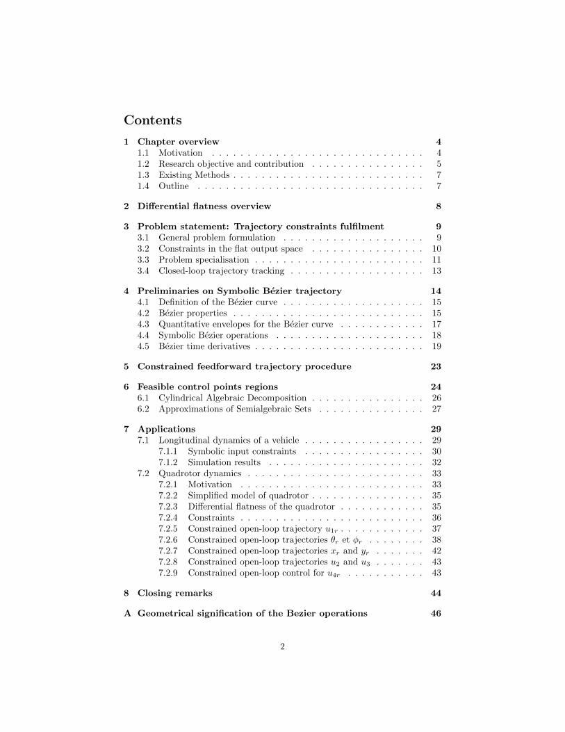
Figure 1: Two degrees of freedom control scheme overview

immediately in front of it. Regarding the complexity of the problem, searchingfor a feasible trajectory is easier, especially in the case where we need real-timere-planning [26, 27]. Considering that the evolution of transistor technologies isreaching its limits, low-complexity controllers that can take the constraints intoaccount are of considerable interest. The same remark is valid when the systemhas sensors with limited performance.

1.2 Research objective and contribution

In this chapter, we propose a novel trajectory-based framework to deal withsystem constraints. We are answering the following question:

Question 1 How to design a set of the reference trajectories (or the feed-forwarding trajectories) of a nonlinear system such that the input, state and/oroutput constraints are fulfilled?

For that purpose, we divide the control problem in two stages (see Figure 1).Our objective will be to elaborate a constrained reference trajectory management(Stage A) which is meant to be applied to already pre-stabilized systems (StageB).

5

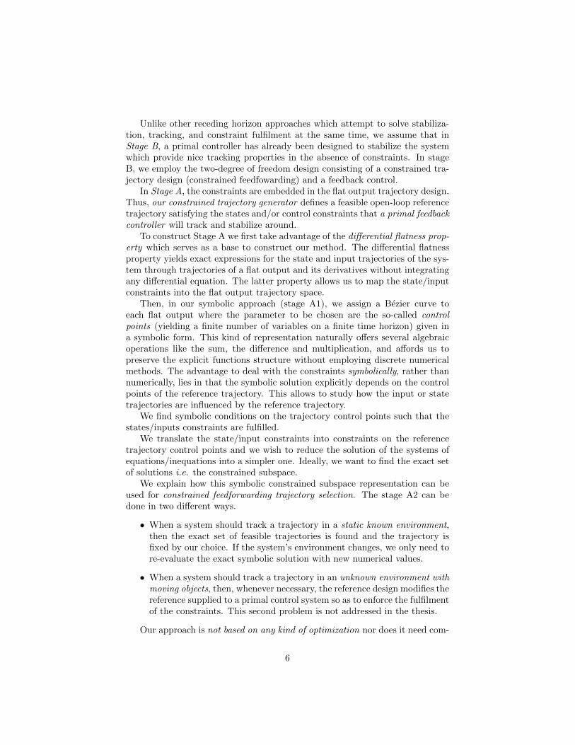
Unlike other receding horizon approaches which attempt to solve stabiliza-tion, tracking, and constraint fulfilment at the same time, we assume that inStage B, a primal controller has already been designed to stabilize the systemwhich provide nice tracking properties in the absence of constraints. In stageB, we employ the two-degree of freedom design consisting of a constrained tra-jectory design (constrained feedfowarding) and a feedback control.

In Stage A, the constraints are embedded in the flat output trajectory design.Thus, our constrained trajectory generator defines a feasible open-loop referencetrajectory satisfying the states and/or control constraints that a primal feedbackcontroller will track and stabilize around.

To construct Stage A we first take advantage of the differential flatness prop-erty which serves as a base to construct our method. The differential flatnessproperty yields exact expressions for the state and input trajectories of the sys-tem through trajectories of a flat output and its derivatives without integratingany differential equation. The latter property allows us to map the state/inputconstraints into the flat output trajectory space.

Then, in our symbolic approach (stage A1), we assign a Bezier curve toeach flat output where the parameter to be chosen are the so-called controlpoints (yielding a finite number of variables on a finite time horizon) given ina symbolic form. This kind of representation naturally offers several algebraicoperations like the sum, the difference and multiplication, and affords us topreserve the explicit functions structure without employing discrete numericalmethods. The advantage to deal with the constraints symbolically, rather thannumerically, lies in that the symbolic solution explicitly depends on the controlpoints of the reference trajectory. This allows to study how the input or statetrajectories are influenced by the reference trajectory.

We find symbolic conditions on the trajectory control points such that thestates/inputs constraints are fulfilled.

We translate the state/input constraints into constraints on the referencetrajectory control points and we wish to reduce the solution of the systems ofequations/inequations into a simpler one. Ideally, we want to find the exact setof solutions i.e. the constrained subspace.

We explain how this symbolic constrained subspace representation can beused for constrained feedforwarding trajectory selection. The stage A2 can bedone in two different ways.

• When a system should track a trajectory in a static known environment,then the exact set of feasible trajectories is found and the trajectory isfixed by our choice. If the system’s environment changes, we only need tore-evaluate the exact symbolic solution with new numerical values.

• When a system should track a trajectory in an unknown environment withmoving objects, then, whenever necessary, the reference design modifies thereference supplied to a primal control system so as to enforce the fulfilmentof the constraints. This second problem is not addressed in the thesis.

Our approach is not based on any kind of optimization nor does it need com-

6

putations for a given numerical value at each sampling step. We determine a setof feasible trajectories through the system constrained environment that enablea controller to make quick real-time decisions. For systems with singularities,we can isolate the singularities of the system by considering them as additionalconstraints.

1.3 Existing Methods

• Considering actuator constraints based on the derivatives of the flat output(for instance, the jerk [22, 53], snap [38]) can be too conservative for somesystems. The fact that a feasible reference trajectory is designed followingthe system model structure allows to choose a quite aggressive referencetrajectory.

• In contrast to [51], we characterize the whose set of viable reference tra-jectories which take the constraints into account.

• In [47], the problem of constrained trajectory planning of differentiallyflat systems is cast into a simple quadratic programming problem ensuingcomputational advantages by using the flatness property and the B-splinescurve’s properties. They simplify the computation complexity by takingadvantage of the B-spline minimal (resp. maximal) control point. Thesimplicity comes at the price of having only minimal (resp. maximal)constant constraints that eliminate the possible feasible trajectories andrenders this approach conservative.

• In [23], an inversion-based design is presented, in which the transition taskbetween two stationary set-points is solved as a two-point boundary valueproblem. In this approach, the trajectory is defined as polynomial whereonly the initial and final states can be fixed.

• The thesis of Bak [2] compared existing methods to constrained controllerdesign (anti-windup, predictive control, nonlinear methods), and intro-duced a nonlinear gain scheduling approach to handle actuator constraints.

1.4 Outline

This chapter is organized as follows:

• In section 2, we recall the notions of differential flatness for finite dimen-sional systems.

• In section 3, we present our problem statement for the constraints fulfil-ment through the reference trajectory.

• In section 4, we detail the flat output parameterization given by the Beziercurve, and its properties.

7

• In section 5, we give the whole procedure in establishing reference tra-jectories for constrained open-loop control. We illustrate the procedurethrough two applications in section 7.

• In section 6, we present the two methods that we have used to computethe constrained set of feasible trajectories.

2 Differential flatness overview

The concept of differential flatness was introduced in [20, 19] for non-linear finitedimensional systems. By the means of differential flatness, a non-linear systemcan be seen as a controllable linear system through a dynamical feedback.

A model shall be described by a differential system as:

x = f(x,u) (1)

where x ∈ Rn denote the state variables and u ∈ Rm the input vector. Sucha system is said to be flat if there exists a set of flat outputs (or linearizingoutputs) (equal in number to the number of inputs) given by

y = h(x,u, u, ...,u(r)) (2)

with r ∈ N such that the components of y ∈ Rm and all their derivatives arefunctionally independent and such that we can parametrize every solution (x,u)of (1) in some dense open set by means of the flat output y and its derivativesup to a finite order q:

x = ψ(y, y, ...,y(q−1)), (3a)

u = ζ(y, y, ...,y(q)) (3b)

where (ψ, ζ) are smooth functions that give the trajectories of x and u as func-tions of the flat outputs and their time derivatives. The preceding expressions in(3), will be used to obtain the so called open-loop controls. The differential flat-ness found numerous applications, non-holonomic systems, among others (see[45] and the references therein).

In the context of feedforwarding trajectories, the “degree of continuity” orthe smoothness of the reference trajectory (or curve) is one of the most im-portant factors. The smoothness of a trajectory is measured by the number ofits continuous derivatives. We give the definitions on the trajectory continuitywhen it is represented by a parametric curve in the Appendix B.

8

3 Problem statement: Trajectory constraints ful-filment

Notation

Given the scalar function z ∈ Cκ(R,R) and the number α ∈ N, we denote byz〈α〉 the tuple of derivatives of z up to the order α 6 κ: z〈α〉 = z, z, z, . . . , z(α).Given the vector function v = (v1, . . . , vq), vi ∈ Cκ(R,R) and the tuple α =(α1, . . . , αq), αi ∈ N, we denote by v〈α〉 the tuple of derivatives of each compo-

nent vi of v up to its respective order αi 6 κ: v〈α〉 = v1, . . . , v(α1)1 , v2, . . . , v

(α2)2 , . . . , vq, . . . , v

(αq)q .

3.1 General problem formulation

Consider the nonlinear system

x(t) = f(x(t),u(t)) (4)

with state vector x = (x1, . . . , xn) and control input u = (u1, . . . , um), xi, uj ∈Cκ([0,+∞),R) for a suitable κ ∈ N. We assume the state, the input and theirderivatives to be subject to both inequality and equality constraints of the form

Ci(x〈αxi 〉(t),u〈α

ui 〉(t)) 6 0 ∀t ∈ [0, T ], ∀i ∈ {1, . . . , νin} (5a)

Dj(x〈βxj 〉(t),u〈β

uj 〉(t)) = 0 ∀t ∈ Ij , ∀j ∈ {1, . . . , νeq} (5b)

with each Ij being either [0, T ] (continuous equality constraint) or a discrete set{t1, . . . , tγ}, 0 ≤ t1 6 · · · 6 tγ 6 T < +∞ (discrete equality constraint), andαxi , β

xj ∈ Nn, αui , β

uj ∈ Nm. We stress that the relations (5) specify objectives

(and constraints) on the finite interval [0, T ]. Objectives can be also formulatedas a concatenation of sub-objectives on a union of sub-intervals, provided thatsome continuity and/or regularity constraints are imposed on the boundaries ofeach sub-interval. Here we focus on just one of such intervals.

Our aim is to characterise the set of input and state trajectories (x,u)satisfying the system’s equations (4) and the constraints (5). More formally westate the following problem.

Problem 1 (Constrained trajectory set) Let C be a subspace of Cκ([0,+∞),R).Constructively characterise the set C cons ⊆ C n+m of all extended trajectories(x,u) satisfying the system (4) and the constraints (5).

Problem 1 can be considered as a generalisation of a constrained reachabilityproblem (see for instance [17]). In such a reachability problem the stress isusually made on initial and final set-points and the goal is to find a suitableinput to steer the state from the initial to the final point while possibly fulfillingthe constraints. Here, we wish to give a functional characterisation of the overallset of extended trajectories (x,u) satisfying some given differential constraints.A classical constrained reachability problem can be cast in the present formalism

9

by limiting the constraints Ci and Dj to x and u (and not their derivatives)and by forcing two of the equality constraints to coincide with the initial andfinal set-points.

Problem 1 is difficult to be addressed in its general setting. To simplifythe problem, in the following we make some restrictions to the class of systemsand to the functional space C . As a first assumption we limit the analysis todifferentially flat systems [20].

3.2 Constraints in the flat output space

Let us assume that system (4) is differentially flat with flat output2

y = (y1, . . . , ym) = h(x,u〈ρu〉) , (6)

with ρu ∈ Nm. Following Equation (3), the parameterisation or the feedfor-warding trajectories associated to the reference trajectory yr is

xr = ψ(yr〈ηx〉) (7a)

ur = ζ(yr〈ηu〉) , (7b)

with ηx ∈ Nn and ηu ∈ Nm.Through the first step of the dynamical extension algorithm [18], we get the

flat output dynamics y

(k1)1 = φ1(y〈µ

y1〉,u〈µ

u1 〉)

...

y(km)m = φm(y〈µ

ym〉,u〈µ

um〉) ,

(8)

with µyi = (µyi1, . . . , µyim) ∈ Nm, µui = (µui1, . . . , µ

uim) ∈ Nm and ki > maxj µ

yji.

The original n-dimensional dynamics (4) and the K-dimensional flat outputdynamics (8) (K =

∑i ki) are in one-to-one correspondence through (6) and

(7). Therefore, the constraints (5) can be re-written as

Γi(yr〈ωini 〉) 6 0 ∀t ∈ [0, T ], ∀i ∈ {1, . . . , νin} (9a)

∆j(yr〈ωeqj 〉) = 0 ∀t ∈ Ij , ∀j ∈ {1, . . . , νeq} (9b)

withΓi(yr

〈ωini 〉) = Ci((ψ(yr

〈ηx 〉))〈αxi 〉, ζ(yr

〈ηu〉)〈αui 〉),

∆j(yr〈ωeqj 〉) = Dj((ψ(yr

〈ηx〉)〈βxj 〉, ζ(yr

〈ηu〉)〈βuj 〉)

and ωini , ω

eqj ∈ Nm.

2We recall that the flat output y has the same dimension m as the input vector u.

10

Remark 1 We may use the same result to embed an input rate constraint ur.

Thus, Problem 1 can be transformed in terms of the flat output dynamics(8) and the constraints (9) as follows.

Problem 2 (Constrained flat output set) 3 Let Cy be a subspace of Cp([0,+∞),R)with p = max((k1, . . . , km), ωin

1 , . . . , ωinνin , ω

eq1 , . . . , ω

eqνeq). Constructively charac-

terise the set C consy ⊆ Cm

y of all flat outputs satisfying the dynamics (8) and theconstraints (9).

Working with differentially flat systems allows us to translate, in a unified fash-ion, all the state and input constraints as constraints in the flat outputs and theirderivatives (See (9)). We remark that ψ and ζ in (7) are such that ψ(y〈ηx〉) andζ(y〈ηu〉) satisfy the dynamics of system (4) by construction. In other words,the extended trajectories (x,u) of (4) are in one-to-one correspondence withy ∈ Cm

y given by (6). Hence, choosing y solution of Problem 2 ensures that xand u given by (7) are solutions of Problem 1.

3.3 Problem specialisation

For any practical purpose, one has to choose the functional space Cy to whichall components of the flat output belong. Instead of making reference to thespace C gen := Cp([0,+∞),R), mentioned in the statement of Problem 1, wefocus on the space C gen

T := Cp([0, T ],R). Indeed, the constraints (9) specifyfinite-time objectives (and constraints) on the interval [0, T ]. Still, the problemexhibits an infinite dimensional complexity, whose reduction leads to choose anapproximation space C app that is dense in C gen

T . A possible choice is to workwith parametric functions expressed in terms of basis functions like, for instance,Bernstein-Bezier, Chebychev or Spline polynomials.

A scalar Bezier curve of degree N ∈ N in the Euclidean space R is definedas

P (s) =

N∑j=0

αjBjN (s), s ∈ [0, 1]

where the αj ∈ R are the control points and BjN (s) =(Nj

)(1 − s)N−jsj are

Bernstein polynomials [13]. For sake of simplicity, we set here T = 1 and wechoose as functional space

C app =

{N∑0

αjBjN |N ∈ N, (αj)N0 ∈ RN+1, Bj ∈ C0([0, 1],R)

}(10)

The set of Bezier functions of generic degree has the very useful property ofbeing closed with respect to addition, multiplication, degree elevation, deriva-tion and integration operations (see section 4). As a consequence, any poly-nomial integro-differential operator applied to a Bezier curve, still produces a

3Here the max operator is applied elementwise on each vector.

11

Bezier curve (in general of different degree). Therefore, if the flat outputs y arechosen in C app and the operators Γi(·) and ∆j(·) in (9) are integro-differentialpolynomials, then such constraints can still be expressed in terms of Beziercurves in C app. We stress that, if some constraints do not admit such a descrip-tion, we can still approximate them up to a prefixed precision ε as function inC app by virtue of the denseness of C app in C gen

1 . Hence we assume the following.

Assumption 1 Considering each flat output yr ∈ C app defined as

yr =

N∑j=0

αjBjN (s),

the constraints (9) can be written as

Γi(yr〈ωini 〉) =

N ini∑

k=0

λikBkN (s), (11)

∆j(yr〈ωeqj 〉) =

Neqi∑

k=0

δjkBkN (s) (12)

where

λik = rinik(α0, . . . , αN )

δjk = reqjk(α0, . . . , αN )

rinik, r

eqjk ∈ R[α0, . . . , αN ]

i.e. the λik and δjk are polynomials in the α0, . . . , αN .�

Set the following expressions asνin

rin = (rin1,0, . . . , r

inνin,Nin

νin),

req = (req1,0, . . . , r

eqνeq,Neq

νeq),

r = (rin, req),

the control point vector α = (α1, . . . , αN ), and the basis function vector B =(B1N , . . . , BNN ). Therefore, we obtain a semi-algebraic set defined as:

I (r,A) ={α ∈ A | rin(α) 6 0, req(α) = 0

}for any parallelotope

A = [α0, α0]× · · · × [αN , αN ], αi, αi ∈ R ∪ {−∞,∞}, αi < αi (13)

Thus I (r,A) is a semi-algebraic set associated to the constraints (9). Theparallelotope A represents the trajectory sheaf of available trajectories, amongwhich the user is allowed to choose a reference. The semi-algebraic set I (r,A)

12

represents how the set A is transformed in such a way that the trajectoriesfulfill the constraints (9). Then, picking an α in I (r,A) ensures that yr = αBautomatically satisfies the constraints (9).The Problem 2 is then reformulated as :

Problem 3 For any fixed parallelotope A, constructively characterise the semi-algebraic set I (r,A).

This may be done through exact, symbolic techniques (such as, e.g. the Cylidri-cal Algebraic Decomposition) or through approximation techniques yieldingouter approximations I out

l (r,A) ⊇ I (r,A) and inner approximations I innl (r,A) ⊆

I (r,A) with liml→∞

I outl = lim

l→∞I innl = I . �

This characterisation shall be useful to extract inner approximations of a specialtype yielding trajectory sheaves included in I (r,A). A specific example of thistype of approximations will consist in disjoint unions of parallelotopes:

I innl (r,A) =

⋃j∈Il

Bl,j , ∀i, j ∈ Il,Bl,i ∩ Bl,j = ∅ (14)

This class of inner approximation is of practical importance for end users,as the applications in Section 7 illustrate.

3.4 Closed-loop trajectory tracking

So far this chapter has focused on the design of open-loop trajectories whileassuming that the system model is perfectly known and that the initial con-ditions are exactly known. When the reference open-loop trajectories (xr,ur)are well-designed i.e. respecting the constraints and avoiding the singularities,as discussed above, the system is close to the reference trajectory. However, tocope with the environmental disturbances and/or small model uncertainties, thetracking of the constrained open-loop trajectories should be made robust usingfeedback control. The feedback control guarantees the stability and a certainrobustness of the approach, and is called the second degree of freedom of theprimal controller (Stage B2 in figure 1).

We recall that some flat systems can be transformed via endogenous feedbackand coordinate change to a linear dynamics [20, 45]. To make this chapter self-contained, we briefly discuss the closed-loop trajectory tracking as presented in[36].

Consider a differentially flat system with flat output y = (y1, . . . , ym) (mbeing the number of independent inputs of the system). Let yr(t) ∈ Cη(R)be a reference trajectory for y. Suppose the desired open-loop state/ inputtrajectories (xr(t), ur(t)) are generated offline. We need now a feedback controlto track them.

Since the nominal open-loop control (or the feedforward input) linearizes thesystem, we can take a simple linear feedback, yielding the following closed-loop

13

error dynamics:

e(η) + λη−1e(η−1) + · · ·+ λ1e+ λ0e = 0 (15)

where e = y − yr is the tracking error and the coefficients Λ = [λ0, . . . , λη−1]are chosen to ensure an asymptotically stable behaviour (see e.g. [19]).

Remark 2 Note that this is not true for all flat systems, in [24] can be foundan example of flat system with nonlinear error dynamics.

Now let (x,u) be the closed-loop trajectories of the system. These variablescan be expressed in terms of the flat output y as:

x = ψ(y〈η−1〉), u = ζ(y〈η〉) (16)

Then, the associated reference open-loop trajectories (xr,ur) are given by

xr = ψ(yr〈η−1〉), ur = ζ(yr

〈η〉)

Therefore,

x = ψ(y〈η−1〉) = ψ(yr〈η−1〉 + e〈η−1〉)

and

u = ζ(y〈η〉) = ζ(yr〈η〉 + e〈η〉,−Λe〈η〉).

As further demonstrated in [36][See Section 3.3], since the tracking errore→ 0 as t→∞ that means x→ xr and u→ ur.

Besides the linear controller (Equation (15)), many different linear and non-linear feedback controls can be used to ensure convergence to zero of the track-ing error. For instance, sliding mode control, high-gain control, passivity basedcontrol, model-free control, among others.

Remark 3 An alternative method to the feedback linearization, is the exactfeedforward linearization presented in [25] where the problem of type ”divisionby zero” in the control design is easily avoided. This control method removes theneed for asymptotic observers since in its design the system states informationis replaced by their corresponding reference trajectories. The robustness of theexact feedforwarding linearization was analyzed in [27].

4 Preliminaries on Symbolic Bezier trajectory

To create a trajectory that passes through several points, we can use approx-imating or interpolating approaches. The interpolating trajectory that passesthrough the points is prone to oscillatory effects (more unstable), while theapproximating trajectory like the Bezier curve or B-Spline curve is more con-venient since it only approaches defined so-called control points [13] and have

14

simple geometric interpretations. The Bezier/B-spline curve can be handled byconveniently handling the curve’s control points.The main reason in choosing the Bezier curves over the B-Splines curves, is thesimplicity of their arithmetic operators presented further in this Section. Despitethe nice local properties of the B-spline curve, the direct symbolic multiplica-tion4 of B-splines lacks clarity and has partly known practical implementation[39].

In the following Section, we start by presenting the Bezier curve and its prop-erties. Bezier curves are chosen to construct the reference trajectories because oftheir nice properties (smoothness, strong convex hull property, derivative prop-erty, arithmetic operations). They have their own type basis function, known asthe Bernstein basis, which establishes a relationship with the so-called controlpolygon. A complete discussion about Bezier curves can be found in [41]. Here,some basic and key properties are recalled as a preliminary knowledge.

4.1 Definition of the Bezier curve

A Bezier curve is a parametric one that uses the Bernstein polynomials as abasis. An nth degree Bezier curve is defined by

f(t) =

N∑j=0

cjBj,N (t), 0 6 t 6 1 (17)

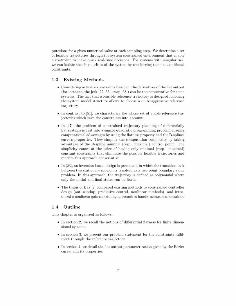
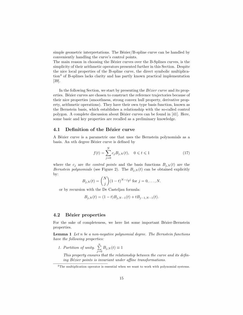
where the cj are the control points and the basis functions Bj,N (t) are theBernstein polynomials (see Figure 2). The Bj,N (t) can be obtained explicitlyby:

Bj,N (t) =

(N

j

)(1− t)N−jtj for j = 0, . . . , N.

or by recursion with the De Casteljau formula:

Bj,N (t) = (1− t)Bj,N−1(t) + tBj−1,N−1(t).

4.2 Bezier properties

For the sake of completeness, we here list some important Bezier-Bernsteinproperties.

Lemma 1 Let n be a non-negative polynomial degree. The Bernstein functionshave the following properties:

1. Partition of unity.n∑j=0

Bj,N (t) ≡ 1

This property ensures that the relationship between the curve and its defin-ing Bezier points is invariant under affine transformations.

4The multiplication operator is essential when we want to work with polynomial systems.

15

j = 2j = 3

j = 4j = 0

j = 1

0.0 0.2 0.4 0.6 0.8 1.0

0.0

0.2

0.4

0.6

0.8

1.0

Figure 2: Bernstein Basis for degree N = 4.

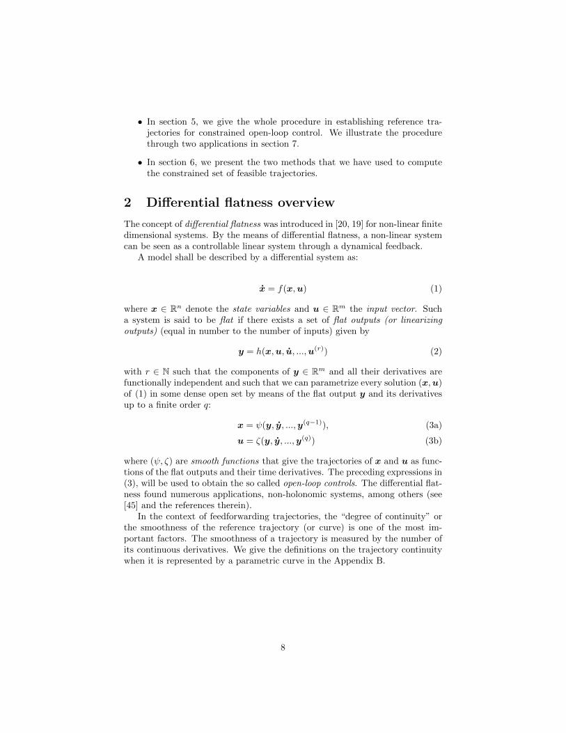
C4

C2

C0

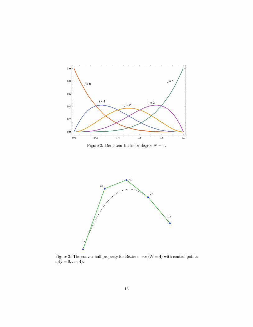
Figure 3: The convex hull property for Bezier curve (N = 4) with control pointscj(j = 0, . . . , 4).

16

2. Positivity. If t ∈ [0, 1] then Bj,N (t) > 0.It guarantees that the curve segment lies completely within the convex hullof the control points (see Figure 3).

3. Tangent property. For the start and end point, this guarantees f(0) = c0and f(1) = cN but the curve never passes through the intermediate controlpoints.

4. Smoothness. Bj,N (t) is N − 1 times continuously differentiable. Hence,increasing degree increases regularity.

4.3 Quantitative envelopes for the Bezier curve

Working with the Bezier curve control points in place of the curve itself allowsa simpler explicit representation. However, since our framework is not based onthe Bezier curve itself, we are interested in the localisation of the Bezier curvewith respect to its control points, i.e. the control polygon. In this part, wereview a result on sharp quantitative bounds between the Bezier curve and itscontrol polygon [40, 32]. For instance, in the case of a quadrotor (discussed inSection 7.2), once we have selected the control points for the reference trajectory,these envelopes describe the exact localisation of the quadrotor trajectory and itsdistance from the obstacles. These quantitative envelopes may be of particularinterest when avoiding corners of obstacles which traditionally in the literature[42] are modelled as additional constraints or introducing safety margin aroundthe obstacle.

We start by giving the definition for the control polygon.

Definition 1 (Control polygon for Bezier curves (see [40])). Let f =∑Nj=0 cjBj,N (t)

be a scalar-valued Bezier curve. The control polygon Γf =∑Nj=0 cjHj(t) of f

is a piecewise linear function connecting the points with coordinates (t∗j , cj) for

j = 0, . . . , N where the first components t∗j = jN are the Greville abscissae. The

hat functions Hj are piecewise linear functions defined as:

Hj(t) =

t−t∗j−1

t∗j−t∗j−1t ∈ [t∗j−1, t

∗j ]

t∗j+1−tt∗j+1−t∗j

t ∈ [t∗j , t∗j+1]

0 otherwise.

An important detail is the maximal distance between a Bezier segment andits control polygon. For that purpose, we recall a result from [40], where sharpquantitative bounds of control polygon distance to the Bezier curve are given.

Theorem 1 (See [40], Theorem 3.1) Let f =∑Nj=0 cjBj,N be a scalar Bezier

curve and let Γf be its control polygon. Then the maximal distance from f toits control polygon is bounded as:

‖f − Γf‖∞,[0,1] 6 µ∞(N) ‖∆2c‖∞ = Dmax (18)

17

where the constant µ∞(N) =bN/2cdN/2e

2N5 only depends on the degree N and

the second difference of the control points ‖∆2c‖∞ := max0<j<N |∆2cj |.

The jth

second difference of the control point sequence cj for j = 0, . . . , N isgiven by:

∆2cj = cj−1 − 2cj + cj+1.

Based on this maximal distance, Bezier curve’s envelopes are defined as twopiecewise linear functions:

• the lower envelope Γf =∑Nj=0 ejHj =

∑Nj=0(cj −Dmax)Hj and,

• the upper envelope Γf =∑Nj=0 ejHj =

∑Nj=0(cj +Dmax)Hj

such that Γf 6 f 6 Γf .The envelopes are improved by taking e0 = e0 = c0 and eN = eN = cN andthen clipped with the standard Min-Max bounds 6. The Min-Max bounds yieldrectangular envelopes that are defined as

Definition 2 (Min-Max Bounding box (see [41])). Let f =∑Nj=0 cjBj,N be a

Bezier curve. As a consequence of the convex-hull property, a min-max boundingbox is defined for the Bezier curve f as:

min0<j<N

cj 6N∑j=0

cjBj,N 6 max0<j<N

cj .

Remark 4 As we notice, the maximal distance between a Bezier segment andits control polygon is bounded in terms of the second difference of the controlpoint sequence and a constant that depends only on the degree of the polynomial.Thus, by elevating the degree of the Bezier control polygon, i.e. the subdivision(without modifying the Bezier curve), we can arbitrary reduce the distance be-tween the curve and its control polygon.

4.4 Symbolic Bezier operations

In this section, we present the Bezier operators needed to find the Bezier controlpoints of the states and the inputs. Let the two polynomials f(t) (of degree m)and g(t) (of degree n) with control points fj and gj be defined as follows:

f(t) =

m∑j=0

fjBj,m(t), 0 6 t 6 1

g(t) =

n∑j=0

gjBj,n(t), 0 6 t 6 1

5Note that the notationdxe means the ceiling of x, i.e. the smallest integer greater thanor equal to x, and the notationbxc means the floor of x, i.e. the largest integer less than orequal to x.

6Unfortunately the simple Min-Max bounds define very large envelopes when applied solely.

18

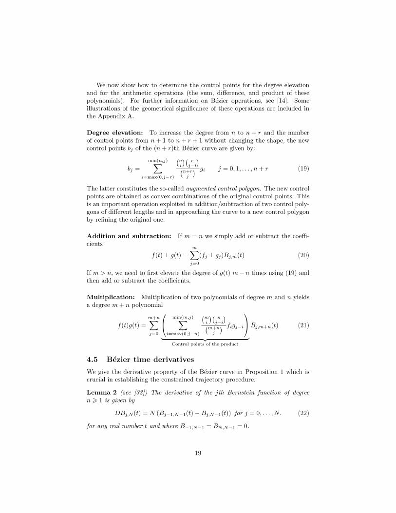
We now show how to determine the control points for the degree elevationand for the arithmetic operations (the sum, difference, and product of thesepolynomials). For further information on Bezier operations, see [14]. Someillustrations of the geometrical significance of these operations are included inthe Appendix A.

Degree elevation: To increase the degree from n to n + r and the numberof control points from n+ 1 to n+ r + 1 without changing the shape, the newcontrol points bj of the (n+ r)th Bezier curve are given by:

bj =

min(n,j)∑i=max(0,j−r)

(ni

)(rj−i)(

n+rj

) gi j = 0, 1, . . . , n+ r (19)

The latter constitutes the so-called augmented control polygon. The new controlpoints are obtained as convex combinations of the original control points. Thisis an important operation exploited in addition/subtraction of two control poly-gons of different lengths and in approaching the curve to a new control polygonby refining the original one.

Addition and subtraction: If m = n we simply add or subtract the coeffi-cients

f(t)± g(t) =

m∑j=0

(fj ± gj)Bj,m(t) (20)

If m > n, we need to first elevate the degree of g(t) m− n times using (19) andthen add or subtract the coefficients.

Multiplication: Multiplication of two polynomials of degree m and n yieldsa degree m+ n polynomial

f(t)g(t) =

m+n∑j=0

min(m,j)∑i=max(0,j−n)

(mi

)(nj−i)(

m+nj

) figj−i

︸ ︷︷ ︸

Control points of the product

Bj,m+n(t) (21)

4.5 Bezier time derivatives

We give the derivative property of the Bezier curve in Proposition 1 which iscrucial in establishing the constrained trajectory procedure.

Lemma 2 (see [33]) The derivative of the jth Bernstein function of degreen > 1 is given by

DBj,N (t) = N (Bj−1,N−1(t)−Bj,N−1(t)) for j = 0, . . . , N. (22)

for any real number t and where B−1,N−1 = BN,N−1 = 0.

19

Proposition 1 If the flat output or the reference trajectory y is a Bezier curve,its derivative is still a Bezier curve and we have an explicit expression for itscontrol points.

Proof 1 Let y(q)(t) denote the qth derivative of the flat output y(t). We usethe fixed time interval T = tf − t0 to define the time as t = Tτ, 0 6 τ 6 1. Wecan obtain y(q)(τ) by computing the qth derivatives of the Bernstein functions.

y(q)(τ) =1

T q

N∑j=0

cjB(q)j,N (τ) (23)

Letting c(0)j = cj, we write

y(τ) = y(0)(τ) =

N∑j=0

c(0)j Bj,N (τ) (24)

Then,

y(q)(τ) =

N−q∑j=0

c(q)j Bj,N−q(τ) (25)

with derivative control points such that

c(q)j =

cj , q = 0

(N − q + 1)

T q

(c(q−1)j+1 − c(q−1)

j

), q > 0.

(26)

We can deduce the explicit expressions for all lower order derivatives up toorder N − 1. This means that if the reference trajectory yr(t) is a Bezier curveof degree N > q (q is the derivation order of the flat output y), by differentiatingit, all states and inputs are given in straightforward Bezier form.

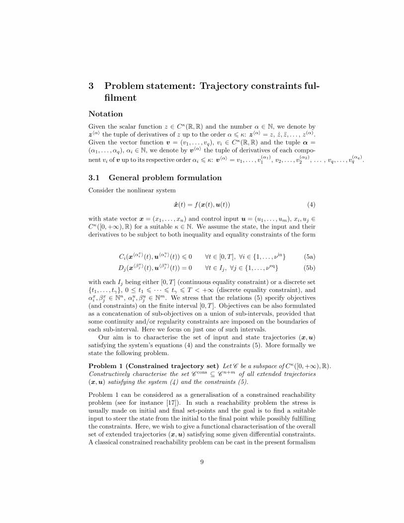
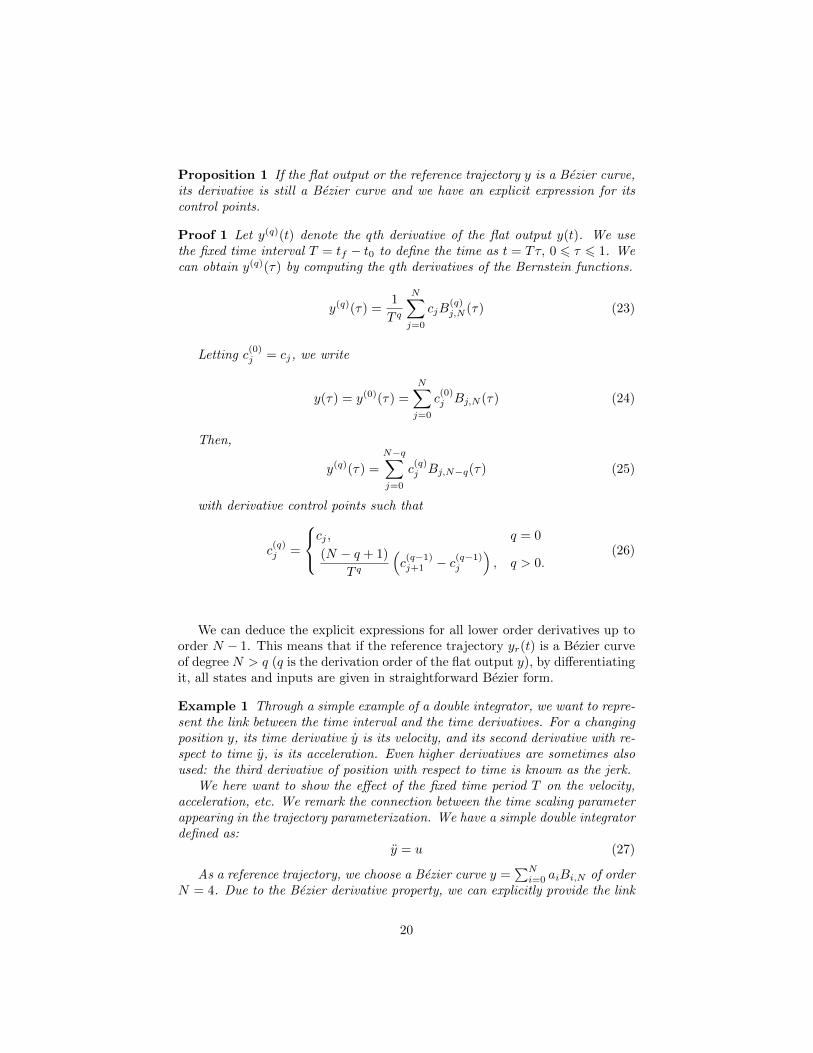
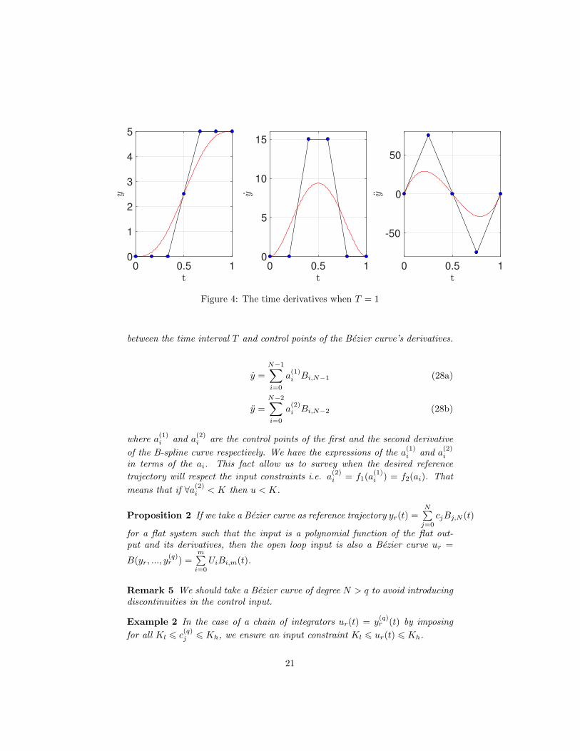
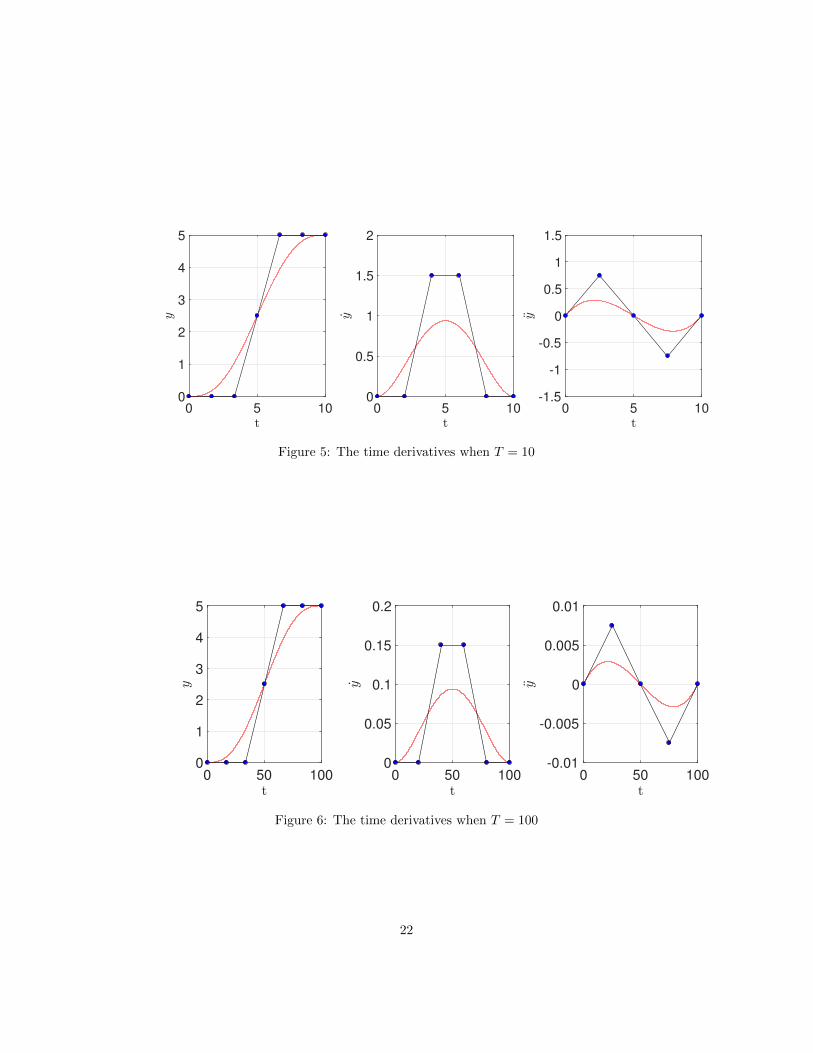
Example 1 Through a simple example of a double integrator, we want to repre-sent the link between the time interval and the time derivatives. For a changingposition y, its time derivative y is its velocity, and its second derivative with re-spect to time y, is its acceleration. Even higher derivatives are sometimes alsoused: the third derivative of position with respect to time is known as the jerk.

We here want to show the effect of the fixed time period T on the velocity,acceleration, etc. We remark the connection between the time scaling parameterappearing in the trajectory parameterization. We have a simple double integratordefined as:

y = u (27)

As a reference trajectory, we choose a Bezier curve y =∑Ni=0 aiBi,N of order

N = 4. Due to the Bezier derivative property, we can explicitly provide the link

20

0 0.5 10

1

2

3

4

5

0 0.5 10

5

10

15

0 0.5 1

-50

0

50

Figure 4: The time derivatives when T = 1

between the time interval T and control points of the Bezier curve’s derivatives.

y =

N−1∑i=0

a(1)i Bi,N−1 (28a)

y =

N−2∑i=0

a(2)i Bi,N−2 (28b)

where a(1)i and a

(2)i are the control points of the first and the second derivative

of the B-spline curve respectively. We have the expressions of the a(1)i and a

(2)i

in terms of the ai. This fact allow us to survey when the desired reference

trajectory will respect the input constraints i.e. a(2)i = f1(a

(1)i ) = f2(ai). That

means that if ∀a(2)i < K then u < K.

Proposition 2 If we take a Bezier curve as reference trajectory yr(t) =N∑j=0

cjBj,N (t)

for a flat system such that the input is a polynomial function of the flat out-put and its derivatives, then the open loop input is also a Bezier curve ur =

B(yr, ..., y(q)r ) =

m∑i=0

UiBi,m(t).

Remark 5 We should take a Bezier curve of degree N > q to avoid introducingdiscontinuities in the control input.

Example 2 In the case of a chain of integrators ur(t) = y(q)r (t) by imposing

for all Kl 6 c(q)j 6 Kh, we ensure an input constraint Kl 6 ur(t) 6 Kh.

21

0 5 100

1

2

3

4

5

0 5 100

0.5

1

1.5

2

0 5 10-1.5

-1

-0.5

0

0.5

1

1.5

Figure 5: The time derivatives when T = 10

0 50 1000

1

2

3

4

5

0 50 1000

0.05

0.1

0.15

0.2

0 50 100-0.01

-0.005

0

0.005

0.01

Figure 6: The time derivatives when T = 100

22

5 Constrained feedforward trajectory procedure

We aim to find a feasible Bezier trajectory (or a set of feasible trajectories, andthen make a suitable choice) yr(t) between the initial conditions yr(t0) = yinitial

and the final conditions yr(tf ) = yfinal. We here show the procedure to obtainthe Bezier control points for the constrained nominal trajectories (yr,xr,ur).

Given a differentially flat system x = f(x,u), the reference design procedurecan be summarized as:

1. Assign to each flat output (trajectory) yi a symbolic Bezier curve yr(t) =N∑j=0

αjBj,N (t) of a suitable degree N > q (q is the time derivatives of the

flat output) and where α = (α0, . . . , αN ) ∈ RN+1 are its control points.

2. Compute the needed derivatives of the flat outputs using Equation (25).

3. Use the Bezier operations to produce the system model relationships (11)-

(12), and to find the state reference Bezier curve xr(t) =m∑i=0

XiBi,m(t)

and input reference Bezier curve ur(t) =m∑j=0

UjBj,m(t) respectively, such

that (Xi, Uj) = rk(α0, . . . , αN ), k = 0, . . . ,m+ n+ 2) are functions of theoutput control points.

4. If needed, calculate the corresponding augmented control polygons by ele-vating the degree of the original control polygons in order to be closer tothe Bezier trajectory.

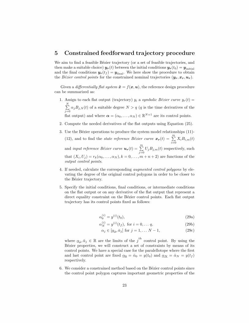
5. Specify the initial conditions, final conditions, or intermediate conditionson the flat output or on any derivative of the flat output that represent adirect equality constraint on the Bezier control points. Each flat outputtrajectory has its control points fixed as follows:

α(i)0 = y(i)(t0), (29a)

α(i)N = y(i)(tf ), for i = 0, . . . q, (29b)

αj ∈ [αj , αj ] for j = 1, . . . N − 1, (29c)

where αj , αj ∈ R are the limits of the jth

control point. By using theBezier properties, we will construct a set of constraints by means of itscontrol points. We have a special case for the paralellotope where the firstand last control point are fixed α0 = α0 = y(t0) and αN = αN = y(tf )respectively.

6. We consider a constrained method based on the Bezier control points sincethe control point polygon captures important geometric properties of the

23

Bezier curve shape. The conditions on the output Bezier control pointsαj , the state Bezier control points Xi and the the input control pointsUj result in a semi-algebraic set (system of polynomial equations and/orinequalities) defined as:

I (r,A) = {α ∈ A | rk(α) ∗k 0, k ∈ {1, . . . , l} , ∗k ∈ {<,6, >,>,=, 6=}}(30)

Depending on the studied system, the output constraints can be definedas in equation (13), or remain as A = RN+1.

7. Find the regions of the control points αj , j = 1, . . . N − 1, solving thesystem of equality/inequalities (30) by using an appropriate method. Wepresent two kind of possible methods in Section 6.

6 Feasible control points regions

Once we transform all the system trajectories through the symbolic Bezier flatoutput, the problem is formulated as a system of functions (equations and in-equalities) with Bezier control points as parameters (see equation (30)). Con-sequently the following question raises:

Question 2 How to find the regions in the space of the parameters (Beziercontrol points) where the system of functions remains valid i.e. the constrainedset of feasible feed-forwarding trajectories?

This section has the purpose to answer the latter question by reviewing twomethods from semialgebraic geometry 7 :

In the first method, we formulate the regions for the reference trajectorycontrol points search as a Quantifier Elimination (QE) problem. The QE is apowerful procedure to compute an equivalent quantifier-free formula for a givenfirst-order formula over the reals [48, 11]. Here we briefly introduce the QEmethod.Let fi(X,U) ∈ Q[X,U ], i = 1, . . . , l be polynomials with rational coefficientswhere:

• X = (x1, . . . , xn) ∈ Rn is a vector of quantified variables

• U = (u1, . . . , um) ∈ Rm is a vector of unquantified (free) variables.

The quantifier-free Boolean formula ϕ(X,U) is a combined expression of poly-nomial equations (fi(X,U) = 0) , inequalities (fi(X,U) ≤ 0), inequations(fi(X,U) 6= 0) and strict inequalities (fi(X,U) > 0) that employs the logic

7The theory that studies the real-number solutions to algebraic inequalities with-real num-ber coefficients, and mappings between them, is called semialgebraic geometry.

24

operators ∧ (and), ∨ (or), ⇒ (implies) or ⇔ (equivalence).A prenex or first-order formula is defined as follows:

G(X,U) = (Q1x1) . . . (Qnxn)[ϕ(X,U)]

where Qi is one of the quantifiers ∀(for all) and ∃ (there exists). Following theTarski Seidenberg theorem (see [11]), for every prenex formula G(X,U) thereexists an equivalent quantifier-free formula ψ(U) defined by the free variables.

The goal of the QE procedure is to compute an equivalent quantifier freeformula ψ(U) for a given first-order formula. It finds the feasible regions of freevariables U represented as semialgebraic set where G(X,U) is true. If the set Uis non-empty, there exists a point u ∈ Rm which simultaneously satisfies all ofthe equations/inequalities. Such a point is called a feasible point and the set Uis then called feasible. If the set U is empty, it is called unfeasible. In the casewhen m = 0, i.e. when all variables are quantified, the QE procedure decideswhether the given formula is true or false (decision problem). For instance,

• given a first order formula ∀x [x2 + bx + c > 0], the QE algorithm givesthe equivalent quantifier free formula b− 4c < 0;

• given a first order formula ∃x [ax2 + bx + c = 0], the QE algorithm givesthe equivalent quantifier free formula (a 6= 0∧ b2− 4ac ≥ 0)∨ (a = 0∧ b 6=0) ∨ (a = 0 ∧ b = 0 ∧ c = 0).

As we can notice, the quantifier free formulas represent the semi-algebraicsets (the conditions) for the unquantified free variables verifying the first orderformula is true. Moreover, given an input formula without quantifiers, the QEalgorithm produces a simplified formula. For instance (for more examples, see[5]),

• given an input formula (ab 6 0)∧ (a+ b = 0)∧ (b2 + a2 > 0)∨ (a2 = −b2),the QE algorithm gives the equivalent simplified formula a+ b = 0.

On the other hand, given an input formula without unquantified free variables(usually called closed formula) is either true or false.

The symbolic computation of the Cylindrical Algebraic Decomposition (CAD)introduced by Collins [10] is the best currently known QE algorithm for solvingreal algebraic constraints (in particular parametric and non-convex case) (see[46]). This method gives us an exact solution, a simplified formula describingthe semi-algebraic set.

The QE methods, particularly the CAD, have already been used in variousaspects of control theory (see [43, 1] and the references therein): robust con-trol design, finding the feasible regions of a PID controller, the Hurwitz andSchur stability regions, reachability analysis of nonlinear systems, trajectorygeneration [30].

25

Remark 6 (On the complexity) Unfortunately the above method rapidly be-comes slow due to its double exponential complexity [34]. Its efficiency stronglydepends on the number and on the complexity of the variables (control points)used for a given problem. The computational complexity of the CAD is doubleexponential i.e. bounded by (sd)2O(n) for a finite set of s polynomials in n vari-ables, of degree d. There are more computationally efficient QE methods thanthe CAD, like the Critical Point Method [4] (it has single exponential complexityin n the number of variables) and the cylindrical algebraic sub-decompositions[52] but to the author knowledge there are no available implementations.

For more complex systems, the exact or symbolic methods are too compu-tationally expensive. There exist methods that are numerical rather than exact.

As a second alternative method, we review one such method based on ap-proximation of the exact set with more reasonable computational cost. Thesecond method known as the Polynomial Superlevel Set (PSS) method, basedon the paper [12] instead of giving us exact solutions tries to approximate theset of solutions by minimizing the L1 norm of the polynomial. It can deal withmore complex problems.

6.1 Cylindrical Algebraic Decomposition

In this section, we give a simple introduction to the Cylindrical Algebraic De-composition.

Input of CAD: As an input of the CAD algorithm, we define a set of poly-nomial equations and/or inequations in n unknown symbolic variables (in ourcase, the control points) defined over real interval domains.

Definition of the CAD: The idea is to develop a sequence of projections thatdrops the dimension of the semi-algebraic set by one each time. Given a set Sof polynomials in Rn, a cylindrical algebraic decomposition is a decompositionof Rn into finitely many connected semialgebraic sets called cells, on whicheach polynomial has constant sign, either +, − or 0. To be cylindrical, thisdecomposition must satisfy the following condition: If 1 6 k < n and π is theprojection from Rn onto Rn−k consisting in removing the k last coordinates,then for every pair of cells c and d, one has either π(c) = π(d) or π(c)∩π(d) = ∅.This implies that the images by π of the cells define a cylindrical decompositionof Rn−k.

Output of CAD: As an output of this symbolic method, we obtain the totalalgebraic expressions that represent an equivalent simpler form of our system.Ideally, we would like to obtain a parametrization of all the control points re-gions as a closed form solution. Finally, in the case where closed forms are com-putable for the solution of a problem, one advantage is to be able to overcome

26

any optimization algorithm to solve the problem for a set of given parameters(numerical values), since only an evaluation of the closed form is then necessary.

The execution runtime and memory requirements of this method dependof the dimension of the problem to be solved because of the computationalcomplexity. For the implementation part, we will use its Mathematica imple-mentation8 (developed by Adam Strzebonski). Other implementations of CADare QEPCAD, Redlog, SyNRAC, Maple.

Example 3 From [28], we present an example in which we want to find theregions of the parameters (a, b) ∈ R2 where the following formula is true, notonly answering if the formula is true or not.Having as input

F ={

(a, b) ∈ R2 : f1(a, b) =√a2 − b2 +

√ab− b2 − a > 0, f2(a, b) = 0 < b < a

}the corresponding CAD output is given by{

a > 0 ∧ b < 4

5a

}As we notice, given a system of equations and inequalities formed by the

control points relationship as an input, the CAD returns a simpler system thatis equivalent over the reals.

6.2 Approximations of Semialgebraic Sets

Here we present a method based on the paper [12] that tries to approximate theset of solutions. Given a set

K = {x ∈ Rn : gi(x) > 0, i = 1, 2, . . . ,m}

which is compact, with non-empty interior and described by given real multi-variable polynomials gi(x) and a compact set B ⊃ K, we aim at determining aso-called polynomial superlevel set (PSS)

U(p) = {x ∈ B : p(x) > 1}

The set B is assumed to be an n-dimensional hyperrectangle. The PSS cancapture the main characteristics of K (it can be non convex and non connected)while having at the same time a simpler description than the original set. It con-sists in finding a polynomial p of degree d whose 1-superlevel set {x | p(x) > 1}contains a semialgebraic set B and has minimum volume. Assuming that one isgiven a simple set B containing K and over which the integrals of polynomialscan be efficiently computed, this method involves searching for a polynomial p

8see https://reference.wolfram.com/language/ref/CylindricalDecomposition.html

27

of degree d which minimizes∫B p(x)dx while respecting the constraints p(x) > 1

on K and p(x) > 0 on B. Note that the objective is linear in the coefficients ofp and that these last two nonnegativity conditions can be made computation-ally tractable by using the sum of squares relaxation. The complexity of theapproximation depends on the degree d. The advantage of such a formulationlies in the fact that when the degree of the polynomial p increases, the objectivevalue of the problem converges to the true volume of the set K.

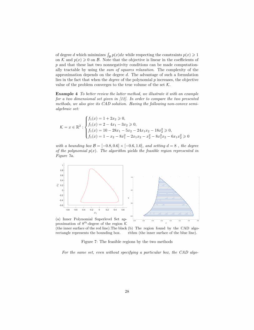
Example 4 To better review the latter method, we illustrate it with an examplefor a two dimensional set given in [12]. In order to compare the two presentedmethods, we also give its CAD solution. Having the following non-convex semi-algebraic set:

K = x ∈ R2 :

f1(x) = 1 + 2x2 > 0,

f1(x) = 2− 4x1 − 3x2 > 0,

f1(x) = 10− 28x1 − 5x2 − 24x1x2 − 18x22 > 0,

f1(x) = 1− x2 − 8x21 − 2x1x2 − x2

2 − 8x21x2 − 6x1x

22 > 0

with a bounding box B = [−0.8, 0.6]× [−0.6, 1.0], and setting d = 8 , the degreeof the polynomial p(x). The algorithm yields the feasible region represented inFigure 7a.

-0.8 -0.6 -0.4 -0.2 0 0.2 0.4 0.6

-0.6

-0.4

-0.2

0

0.2

0.4

0.6

0.8

1

(a) Inner Polynomial Superlevel Set ap-proximation of 8th-degree of the region K(the inner surface of the red line).The blackrectangle represents the bounding box.

-0.8 -0.6 -0.4 -0.2 0.0 0.2 0.4 0.6

-0.5

0.0

0.5

1.0

x1

x2

(b) The region found by the CAD algo-rithm (the inner surface of the blue line).

Figure 7: The feasible regions by the two methods

For the same set, even without specifying a particular box, the CAD algo-

28

ririthm finds the following explicit solution:(x1 = −5

8∧ x2 = −1

2

)∨

(−5

8< x1 < −

1

6∧ −1

26 x2 6

−8x21 − 2x1 − 1

2(6x1 + 1)− 1

2

√64x4

1 − 160x31 − 12x2

1 + 28x1 + 5

(6x1 + 1)2

)

∨(x1 = −1

6∧ −1

26 x2 6

7

8

)∨

(−1

6< x1 <

1

2∧ −1

26 x2 6

−8x21 − 2x1 − 1

2(6x1 + 1)+

1

2

√64x4

1 − 160x31 − 12x2

1 + 28x1 + 5

(6x1 + 1)2

)

∨(x1 =

1

2∧ x2 = −1

2

)As we can observe, the PSS method (Figure 7a) gives us a good approxi-

mation of the feasible region, almost the same as the exact one obtained by theCAD algorithm (Figure 7b). However, in some cases, we observed that the PSSmethod may have some sensibilities when its bounding box is not well defined.

7 Applications

7.1 Longitudinal dynamics of a vehicle

The constraints are essentials in the design of vehicle longitudinal control whichaims to ensure the passenger comfort, safety and fuel/energy reduction. Thelongitudinal control can be designed for a highway scenario or a city scenario.In the first scenario, the vehicle velocity keeps a constant form where the mainobjective is the vehicle inter-distance while the second one, deals with frequentstops and accelerations, the so-called Stop-and-Go scenario [50]. The inter-distance dynamics can be represented as an single integrator driven by the dif-ference between the leader vehicle velocity Vl and the follower vehicle velocityVx , i.e., d = Vl − Vx.In this example, suppose we want to follow the leader vehicle, and stay withina fixed distance from it (measuring the distance through a camera/radar sys-tem). Additionally, suppose we enter a desired destination through a GPSsystem, and suppose our GPS map contains all the speed information lim-its. Our goal is the follower longitudinal speed Vx to follow a reference speedVxr(t) ∈ [0,min(Vl, Vmax)], Vmax ∈ R > 0 given by the minimum between theleader vehicle speed and the speed limit.

The longitudinal dynamics of a follower vehicle is given by the followingmodel:

MVx(t) =u(t)

r− CaV 2

x (t) (31)

where Vx is the longitudinal speed of the vehicle, u is the motor torque, takenas control input and the physical constants: M the vehicle’s mass, r the mean

29

wheel radius, and Ca the aerodynamic coefficient.The model is differentially flat, with Vx as a flat output. An open loop controlyielding the tracking of the reference trajectory Vxr by Vx, assuming the modelto be perfect, is

ur(t) = r(MVxr(t) + CaV

2xr(t)

)(32)

If we desire an open-loop trajectory ur ∈ C0, then for the flat output, we shouldassign a Bezier curve of degree d > 1. We take Vxr as reference trajectory, aBezier curve of degree 4 i.e. C4-function.

Vxr(t) =

4∑i=0

aiBi,4(t),

Vxr(t0) = Vi, Vxr(tf ) = Vf

where the ai’s are the control points and the Bi,4 the Bernstein polynomials.Using the Bezier curve properties, we can find the control points of the open-loopcontrol ur in terms of the ai’s by the following steps:

1. First, we find the control points a(1)i for Vxr by using the Equation (26):

Vxr =

3∑i=0

a(1)i Bi,3(t)

2. We obtain the term V 2xr by

V 2xr =

4∑i=0

aiBi,4(t)

4∑i=0

aiBi,4(t) =

8∑i=0

piBi,8(t)

which is a Bezier curve of degree 8 and where the control points pi arecomputed by the multiplication operation (see Equation (21)).

3. We elevate the degree of the first term up to 8 by using the Equation (19)and then, we find the sum of the latter with the Bezier curve for V 2

xr. Weend up with ur as a Bezier curve of degree 8 with nine control points Ui:

ur(t) = rMVxr+rCaV2xr = rM

3∑i=0

aiBi,3(t)+rCa(

4∑i=0

aiBi,4)2 =

8∑i=0

UiBi,8(t)

with Ui = rk(a0, . . . , a4).

7.1.1 Symbolic input constraints

We want the input control points Ui to be

Umin < Ui < Umax i = 0, . . . , 8 (33)

30

where Umin = 0 is the lower input constraint and Umax = 10 is the high in-put constraint. By limiting the control input, we indirectly constraint thefuel consumption. The initial and final trajectory control points are definedas Vx(t0) = a0 = 0 and Vx(t1) = a4 = 1 respectively.

The constraint (33) directly corresponds to the semi-algebraic set: The con-straint (33) corresponds to the semi-algebraic set i.e. the following system ofnonlinear inequalities:

0 < U0 = 4 a1 < 10

0 < U1 = a1 + 3 a22 < 10

0 < U2 =4 a21

7 −5 a1

7 + 12 a27 + 3 a3

7 < 10

0 < U3 = 15 a214 −

10 a17 + a3 + 6 a1 a2

7 + 114 < 10

0 < U4 =18 a22

35 −10 a1

7 + 10 a37 + 16 a1 a3

35 + 27 < 10

0 < U5 = 10 a37 − 15 a2

14 −6 a1

7 + 6 a2 a37 + 5

7 < 10

0 < U6 =4 a23

7 + 5 a37 −

3 a17 −

9 a27 + 10

7 < 10

0 < U7 = 52 −

3 a22 < 10

0 < U8 = 5− 4 a3 < 10

(34)

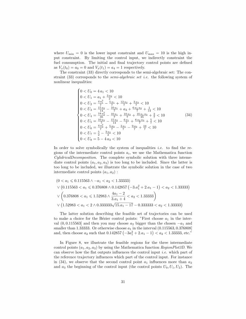
In order to solve symbolically the system of inequalities i.e. to find the re-gions of the intermediate control points ai, we use the Mathematica functionCylidricalDecomposition. The complete symbolic solution with three inteme-diate control points (a1, a2, a3) is too long to be included. Since the latter istoo long to be included, we illustrate the symbolic solution in the case of twointermediate control points (a1, a2) :

(0 < a1 6 0.115563 ∧ −a1 < a2 < 1.33333)

∨(0.115563 < a1 6 0.376808 ∧ 0.142857

(−3.a2

1 + 2.a1 − 1)< a2 < 1.33333

)∨(

0.376808 < a1 6 1.52983 ∧ 4a1 − 2

3.a1 + 4< a2 < 1.33333

)∨(1.52983 < a1 < 2 ∧ 0.333333

√15.a1 − 17− 0.333333 < a2 < 1.33333

)The latter solution describing the feasible set of trajectories can be used

to make a choice for the Bezier control points: ”First choose a1 in the inter-val (0, 0.115563] and then you may choose a2 bigger than the chosen −a1 andsmaller than 1.33333. Or otherwise choose a1 in the interval (0.115563, 0.376808]and, then choose a2 such that 0.142857

(−3a2

1 + 2.a1 − 1)< a2 < 1.33333, etc.”

In Figure 8, we illustrate the feasible regions for the three intermediatecontrol points (a1, a2, a3) by using the Mathematica function RegionPlot3D. Wecan observe how the flat outputs influences the control input i.e. which part ofthe reference trajectory influences which part of the control input. For instancein (34), we observe that the second control point a1 influences more than a2

and a3 the beginning of the control input (the control points U0, U1, U2). The

31

Figure 8: Feasible region for the control points of Vxr when Umin = 0 andUmax = 10.

previous inequalities can be used as a prior study to the sensibility of the controlinputs with respect to the flat outputs.

It should be stressed that the goal here is quite different than the traditionalone in optimisation problems. We do not search for the best trajectory accordingto a certain criterion under the some constraints, but we wish to obtain the setof all trajectories fulfilling the constraints; this for an end user to be able topick one or another trajectory in the set and to switch from one to another inthe same set. The picking and switching operations aim to be really fast.

7.1.2 Simulation results

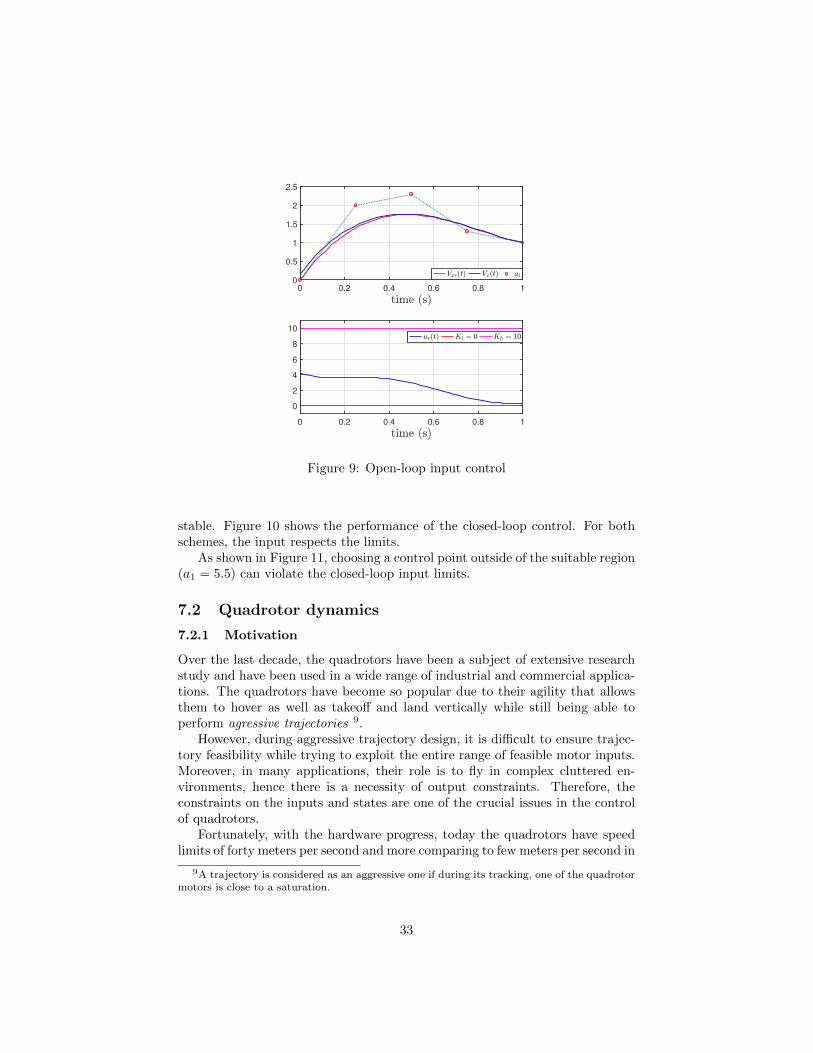
The proposed control approach has been successfully tested in simulation. Forthe physical parameters of the vehicle, academic values are chosen to test theconstraint fulfilment. For the design of the Bezier reference trajectory, we pickvalues for a1, a2 and a3 in the constrained region. As trajectory control pointsfor Vxr, we take the possible feasible choice a0 = 0, a1 = 2, a2 = 2.3, a3 =1.3, a4 = 1. Simulation results for the constrained open-loop input are shownin Figure 9.

The form of the closed-loop input is

u = Mr(Vxr − λ(Vx − Vxr)

)+ rCaV

2x (35)

where λ = 9 is the proportional feedback gain chosen to make the error dynamics

32

0 0.2 0.4 0.6 0.8 1

0

0.5

1

1.5

2

2.5

0 0.2 0.4 0.6 0.8 1

0

2

4

6

8

10

Figure 9: Open-loop input control

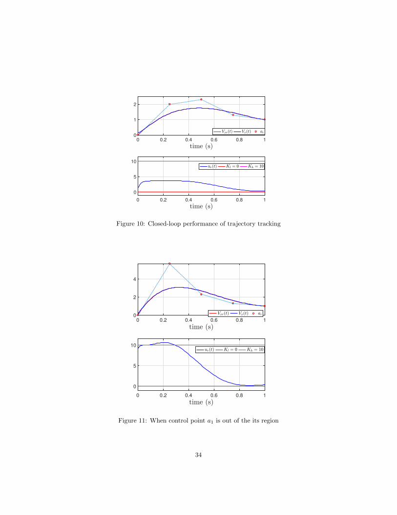
stable. Figure 10 shows the performance of the closed-loop control. For bothschemes, the input respects the limits.

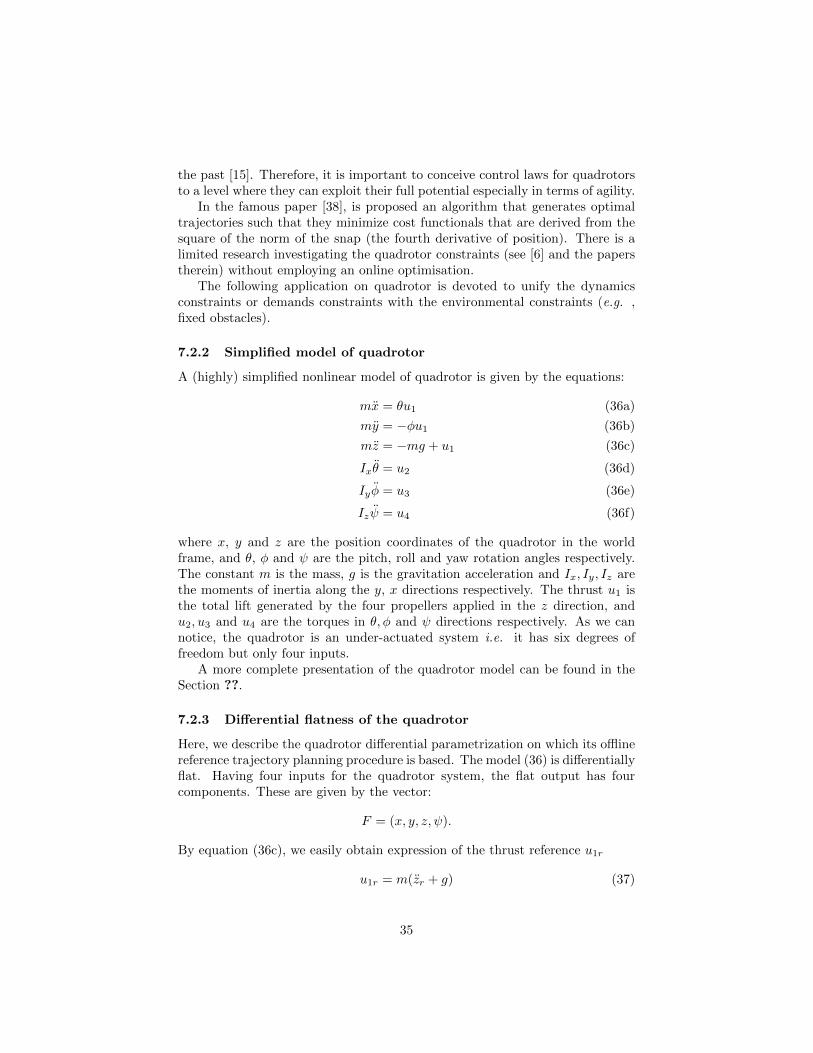
As shown in Figure 11, choosing a control point outside of the suitable region(a1 = 5.5) can violate the closed-loop input limits.

7.2 Quadrotor dynamics

7.2.1 Motivation

Over the last decade, the quadrotors have been a subject of extensive researchstudy and have been used in a wide range of industrial and commercial applica-tions. The quadrotors have become so popular due to their agility that allowsthem to hover as well as takeoff and land vertically while still being able toperform agressive trajectories 9.

However, during aggressive trajectory design, it is difficult to ensure trajec-tory feasibility while trying to exploit the entire range of feasible motor inputs.Moreover, in many applications, their role is to fly in complex cluttered en-vironments, hence there is a necessity of output constraints. Therefore, theconstraints on the inputs and states are one of the crucial issues in the controlof quadrotors.

Fortunately, with the hardware progress, today the quadrotors have speedlimits of forty meters per second and more comparing to few meters per second in

9A trajectory is considered as an aggressive one if during its tracking, one of the quadrotormotors is close to a saturation.

33

0 0.2 0.4 0.6 0.8 1

0

1

2

0 0.2 0.4 0.6 0.8 1

0

5

10

Figure 10: Closed-loop performance of trajectory tracking

0 0.2 0.4 0.6 0.8 1

0

2

4

0 0.2 0.4 0.6 0.8 1

0

5

10

Figure 11: When control point a1 is out of the its region

34

the past [15]. Therefore, it is important to conceive control laws for quadrotorsto a level where they can exploit their full potential especially in terms of agility.

In the famous paper [38], is proposed an algorithm that generates optimaltrajectories such that they minimize cost functionals that are derived from thesquare of the norm of the snap (the fourth derivative of position). There is alimited research investigating the quadrotor constraints (see [6] and the paperstherein) without employing an online optimisation.

The following application on quadrotor is devoted to unify the dynamicsconstraints or demands constraints with the environmental constraints (e.g. ,fixed obstacles).

7.2.2 Simplified model of quadrotor

A (highly) simplified nonlinear model of quadrotor is given by the equations:

mx = θu1 (36a)

my = −φu1 (36b)

mz = −mg + u1 (36c)

Ixθ = u2 (36d)

Iyφ = u3 (36e)

Izψ = u4 (36f)

where x, y and z are the position coordinates of the quadrotor in the worldframe, and θ, φ and ψ are the pitch, roll and yaw rotation angles respectively.The constant m is the mass, g is the gravitation acceleration and Ix, Iy, Iz arethe moments of inertia along the y, x directions respectively. The thrust u1 isthe total lift generated by the four propellers applied in the z direction, andu2, u3 and u4 are the torques in θ, φ and ψ directions respectively. As we cannotice, the quadrotor is an under-actuated system i.e. it has six degrees offreedom but only four inputs.

A more complete presentation of the quadrotor model can be found in theSection ??.

7.2.3 Differential flatness of the quadrotor

Here, we describe the quadrotor differential parametrization on which its offlinereference trajectory planning procedure is based. The model (36) is differentiallyflat. Having four inputs for the quadrotor system, the flat output has fourcomponents. These are given by the vector:

F = (x, y, z, ψ).

By equation (36c), we easily obtain expression of the thrust reference u1r

u1r = m(zr + g) (37)

35

Then, by replacing the thrust expression in (36a)–(36b), we obtain the anglesθr and φr given by

θr =mxru1r

=xr

zr + g(38a)

φr =−myru1r

=−yrzr + g

(38b)

We then differentiate (38a), (38b) and ψr twice to obtain (36d)–(36f) respec-tively. This operation gives us u2 , u3 and u4.

u2r = Ixθr =Ix

(g + zr)

(x(4)r − 2

x(3)r (zr + g)− xrz(3)

r )

(zr + g)2z(3)r −

xrz(4)r

zr + g

), (39)

u3r = Iyφr =Iy

(g + zr)

(−y(4)

r + 2y

(3)r (zr + g)− yrz(3)

r )

(zr + g)2z(3)r +

yrz(4)r

zr + g

), (40)

andu4r = Izψr. (41)

A more complete model of a quadrotor and its flatness parametrization can befound in [44] and [21].

7.2.4 Constraints

Given an initial position and yaw angle and a goal position and yaw angle of thequadrotor, we want to find a set of smooth reference trajectories while respect-ing the dynamics constraints and the environmental constraints. Quadrotorshave electric DC rotors that have limits in their rotational speeds, so input con-straints are vital to avoid rotor damage. Besides the state and input constraints,to enable them to operate in constrained spaces, it is of great importance toimpose output constraints.

We consider the following constraints:

1. The thrust u1

We set a maximum ascent or descending acceleration of 4g (g=9.8 m/s2),and hence the thrust constraint is defined as:

0 < u1 6 Umax1 = 4m·g = 20.79 N, (42)

where m is the quadrotor mass which is set as 0.53 kg in the simulation.By the latter constraint, we also avoid the singularity for a zero thrust.

2. The pitch and roll angleIn applications, the tilt angle is usually inferior to 14 degrees (0.25rad).We set

|φ| 6 Φmax = 0.25rad (43)

|θ| 6 Θmax = 0.25rad (44)

36

3. The torques u2, u3 et u4

With a maximum tilt acceleration of 48 rad/s2, the limits of the controlinputs are:

|u2|, |u3| 6 48Ixx = 0.3 N·m (45)

|u4| 6 48Izz = 0.5 N·m (46)

where Ixx, Iyy, Izz are the parameters of the moment of inertia, Ixx =Iyy=6.22×10−3kg ·m2, Izz = 1.12×10−2kg ·m2.

4. Collision-free constraintTo avoid obstacles, constraints on the output trajectory x, y, z should bereconsidered.

Scenario 1: In this scenario, we want to impose constraints on the thrust,and on the roll and pitch angles.

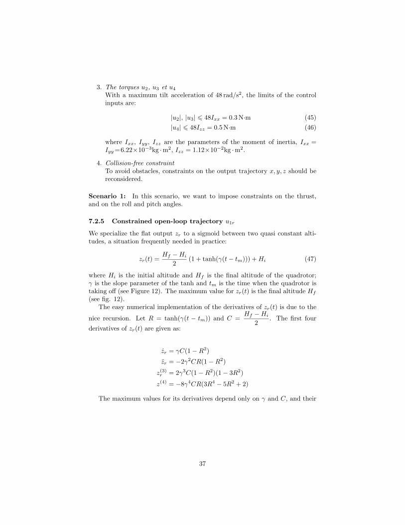
7.2.5 Constrained open-loop trajectory u1r

We specialize the flat output zr to a sigmoid between two quasi constant alti-tudes, a situation frequently needed in practice:

zr(t) =Hf −Hi

2(1 + tanh(γ(t− tm))) +Hi (47)

where Hi is the initial altitude and Hf is the final altitude of the quadrotor;γ is the slope parameter of the tanh and tm is the time when the quadrotor istaking off (see Figure 12). The maximum value for zr(t) is the final altitude Hf

(see fig. 12).The easy numerical implementation of the derivatives of zr(t) is due to the

nice recursion. Let R = tanh(γ(t − tm)) and C =Hf −Hi

2. The first four

derivatives of zr(t) are given as:

zr = γC(1−R2)

zr = −2γ2CR(1−R2)

z(3)r = 2γ3C(1−R2)(1− 3R2)

z(4) = −8γ4CR(3R4 − 5R2 + 2)

The maximum values for its derivatives depend only on γ and C, and their

37

0 2 4 6 8 100

0.5

1

1.5

2

0 2 4 6 8 10

-50

0

50

Figure 12: The reference trajectory for zr(t) (left) and its derivatives (right)with Hi = 0m and Hf = 2m, tm = 5s and parameter γ = 2.

values can be determined. We obtain their bounds as:

Hi 6 zr 6 Hf ,

0 6 zr 6 b1γC, b1 = 1;

−b2γ2C 6zr 6 b2γ2C, b2 =

4√

3

9;

−b3γ3C 6 z(3)r 6 b3γ

3C, b3 =2

3, b3 = 2;

−b4γ4C 6 z(4) 6 b4γ4C, b4 ≈ 4.0849.

Consequently, from the thrust limits (42), we have the following inequality

0 < m(−b2γ2 + g) 6 u1r = m(zr + g) 6 m(b2γ2 + g) < Umax

1 .

The input constraint of u1r will be respected by choosing a suitable value of γand C such that

γ2C < min

{1

b2

(Umax

1

m− g),g

b2

}. (48)

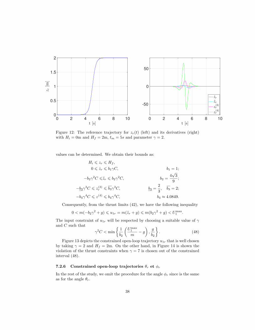
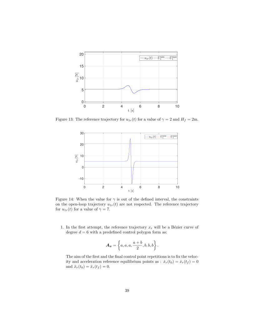
Figure 13 depicts the constrained open-loop trajectory u1r that is well chosenby taking γ = 2 and Hf = 2m. On the other hand, in Figure 14 is shown theviolation of the thrust constraints when γ = 7 is chosen out of the constrainedinterval (48).

7.2.6 Constrained open-loop trajectories θr et φr

In the rest of the study, we omit the procedure for the angle φr since is the sameas for the angle θr.

38

0 2 4 6 8 10

0

5

10

15

20

Figure 13: The reference trajectory for u1r(t) for a value of γ = 2 and Hf = 2m.

0 2 4 6 8 10

-10

0

10

20

30

Figure 14: When the value for γ is out of the defined interval, the constraintson the open-loop trajectory u1r(t) are not respected. The reference trajectoryfor u1r(t) for a value of γ = 7.

1. In the first attempt, the reference trajectory xr will be a Bezier curve ofdegree d = 6 with a predefined control polygon form as:

Ax =

{a, a, a,

a+ b

2, b, b, b

}.

The aim of the first and the final control point repetitions is to fix the veloc-ity and acceleration reference equilibrium points as : xr(t0) = xr(tf ) = 0and xr(t0) = xr(tf ) = 0.

39

The control polygon of the velocity reference trajectory x is :

Ax =

{0, 0,

d

T

b− a2

,d

T

b− a2

, 0, 0

}.

The control polygon of the acceleration reference trajectory x is :

Ax =

{0,d(d− 1)

T 2

a+ b

2, 0,−d(d− 1)

T 2

a+ b

2, 0

}.

The proposed form of Bezier curve provide us the explicit bounds of itssecond derivative xr when a = 0 such that xmin

r = − 14425

bT 2 and xmax

r =14425

bT 2 .

From the Equations (43) and (38a), we get

− 14425

bT 2

b2γ2C + g6 θr =

xrzr + g

614425

bT 2

−b2γ2C + g(49)

0 5 100

5

10

15

20

25

0 5 100

2

4

6

8

0 5 10-4

-2

0

2

4

Figure 15: The Sigmoid Bezier trajectory xr, the velocity trajectory xr and theacceleration trajectory xr with their respective control polygons when a = 0and b = 25.

2. In a second case, the reference trajectory xr can be any Bezier curve.However, we need to impose the first and last controls points in order tofix the initial and final equilibrium states. For the example, we take aBezier trajectory of degree d = 8 with control polygon defined as:

Ax = {a, a, a, α1, α2, α3, b, b, b} .

40

0 2 4 6 8 10

-0.3

-0.2

-0.1

0

0.1

0.2

0.3

Figure 16: The open-loop trajectory θr(t) for Sigmoid Bezier trajectory

When γ = 2 and Hi = 0m, Hf = 2m are fixed, the minimum and maximumvalues for zr are also fixed. Therefore, to impose constraints on θr, it remainsto determine xr, i.e. the control points of xr

xr 6 (−b2γ2C + g)Θmax = Xmax ≈ 1.682m/s2, (50)

xr > −(b2γ2C + g)Θmax = Xmin ≈ −3.222m/s2. (51)

The initial and final trajectory control points are defined as xr(t0) = a = 0and xr(tf ) = b = 2 respectively. Therefore, for xr where T = tf − t0 = 10, weobtain the following control polygon Ax = (axi)

6i=0 :

Ax =

{0,

14α1

25,

14α2 − 28α1

25,

14α1 − 28α2 + 14α3

25,

14α2 − 28α3 + 28

25,

14α3 − 28

25, 0

}.

As explained in the previous section, to reduce the distance between thecontrol polygon and the Bezier curve, we need to elevate the degree of thecontrol polygon Ax. We elevate the degree of Ax up to 16 and we obtain anew augmented control polygon AA

x by using the operation (19) (see Figure 17(right)).

The equation (50) translates into a system of linear inequalities i.e. semi-algebraic set defined as :

Xmin < aAxi = f(α1, α2, α3) < Xmax i = 0, . . . , 16. (52)

We illustrate the feasible regions for the control points by using the Mathe-matica function RegionPlot3D (see Figure 18).

41

0 5 100

2

4

6

8

10

12

14

0 5 10-6

-4

-2

0

2

4

6

8

0 5 10-5

0

5

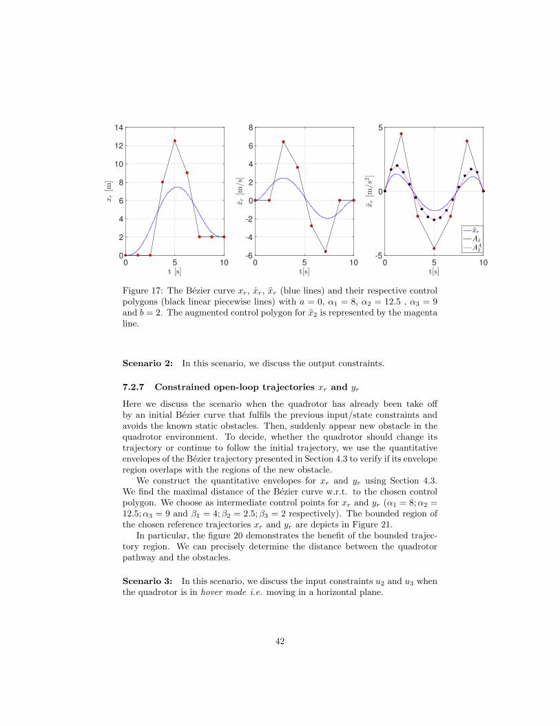
Figure 17: The Bezier curve xr, xr, xr (blue lines) and their respective controlpolygons (black linear piecewise lines) with a = 0, α1 = 8, α2 = 12.5 , α3 = 9and b = 2. The augmented control polygon for x2 is represented by the magentaline.

Scenario 2: In this scenario, we discuss the output constraints.

7.2.7 Constrained open-loop trajectories xr and yr

Here we discuss the scenario when the quadrotor has already been take offby an initial Bezier curve that fulfils the previous input/state constraints andavoids the known static obstacles. Then, suddenly appear new obstacle in thequadrotor environment. To decide, whether the quadrotor should change itstrajectory or continue to follow the initial trajectory, we use the quantitativeenvelopes of the Bezier trajectory presented in Section 4.3 to verify if its enveloperegion overlaps with the regions of the new obstacle.

We construct the quantitative envelopes for xr and yr using Section 4.3.We find the maximal distance of the Bezier curve w.r.t. to the chosen controlpolygon. We choose as intermediate control points for xr and yr (α1 = 8;α2 =12.5;α3 = 9 and β1 = 4;β2 = 2.5;β3 = 2 respectively). The bounded region ofthe chosen reference trajectories xr and yr are depicts in Figure 21.

In particular, the figure 20 demonstrates the benefit of the bounded trajec-tory region. We can precisely determine the distance between the quadrotorpathway and the obstacles.

Scenario 3: In this scenario, we discuss the input constraints u2 and u3 whenthe quadrotor is in hover mode i.e. moving in a horizontal plane.

42

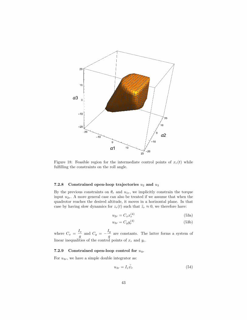
Figure 18: Feasible region for the intermediate control points of xr(t) whilefulfilling the constraints on the roll angle.

7.2.8 Constrained open-loop trajectories u2 and u3

By the previous constraints on θr and u1r, we implicitly constrain the torqueinput u2r. A more general case can also be treated if we assume that when thequadrotor reaches the desired altitude, it moves in a horizontal plane. In thatcase by having slow dynamics for zr(t) such that zr ≈ 0, we therefore have:

u2r = Cxx(4)r (53a)

u3r = Cyy(4)r (53b)

where Cx =Ixg

and Cy = −Iyg

are constants. The latter forms a system of

linear inequalities of the control points of xr and yr.

7.2.9 Constrained open-loop control for u4r

For u4r, we have a simple double integrator as:

u4r = Izψr (54)

43

0 2 4 6 8 10

-0.3

-0.2

-0.1

0

0.1

0.2

0.3

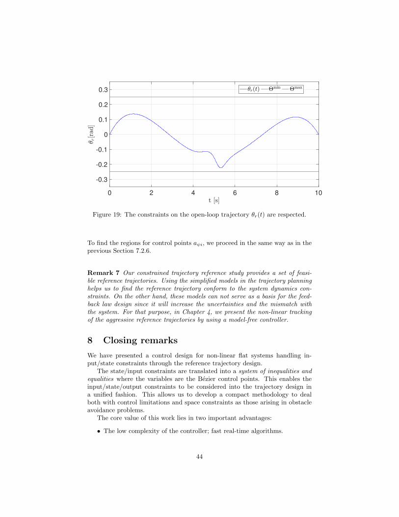
Figure 19: The constraints on the open-loop trajectory θr(t) are respected.

To find the regions for control points aψi, we proceed in the same way as in theprevious Section 7.2.6.

Remark 7 Our constrained trajectory reference study provides a set of feasi-ble reference trajectories. Using the simplified models in the trajectory planninghelps us to find the reference trajectory conform to the system dynamics con-straints. On the other hand, these models can not serve as a basis for the feed-back law design since it will increase the uncertainties and the mismatch withthe system. For that purpose, in Chapter 4, we present the non-linear trackingof the aggressive reference trajectories by using a model-free controller.

8 Closing remarks

We have presented a control design for non-linear flat systems handling in-put/state constraints through the reference trajectory design.

The state/input constraints are translated into a system of inequalities andequalities where the variables are the Bezier control points. This enables theinput/state/output constraints to be considered into the trajectory design ina unified fashion. This allows us to develop a compact methodology to dealboth with control limitations and space constraints as those arising in obstacleavoidance problems.

The core value of this work lies in two important advantages:

• The low complexity of the controller; fast real-time algorithms.

44

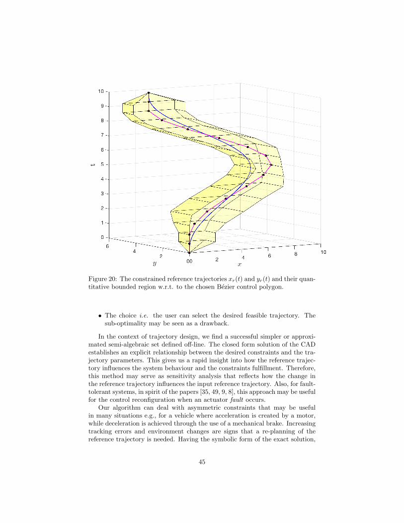
Figure 20: The constrained reference trajectories xr(t) and yr(t) and their quan-titative bounded region w.r.t. to the chosen Bezier control polygon.

• The choice i.e. the user can select the desired feasible trajectory. Thesub-optimality may be seen as a drawback.

In the context of trajectory design, we find a successful simpler or approxi-mated semi-algebraic set defined off-line. The closed form solution of the CADestablishes an explicit relationship between the desired constraints and the tra-jectory parameters. This gives us a rapid insight into how the reference trajec-tory influences the system behaviour and the constraints fulfillment. Therefore,this method may serve as sensitivity analysis that reflects how the change inthe reference trajectory influences the input reference trajectory. Also, for fault-tolerant systems, in spirit of the papers [35, 49, 9, 8], this approach may be usefulfor the control reconfiguration when an actuator fault occurs.

Our algorithm can deal with asymmetric constraints that may be usefulin many situations e.g., for a vehicle where acceleration is created by a motor,while deceleration is achieved through the use of a mechanical brake. Increasingtracking errors and environment changes are signs that a re-planning of thereference trajectory is needed. Having the symbolic form of the exact solution,

45

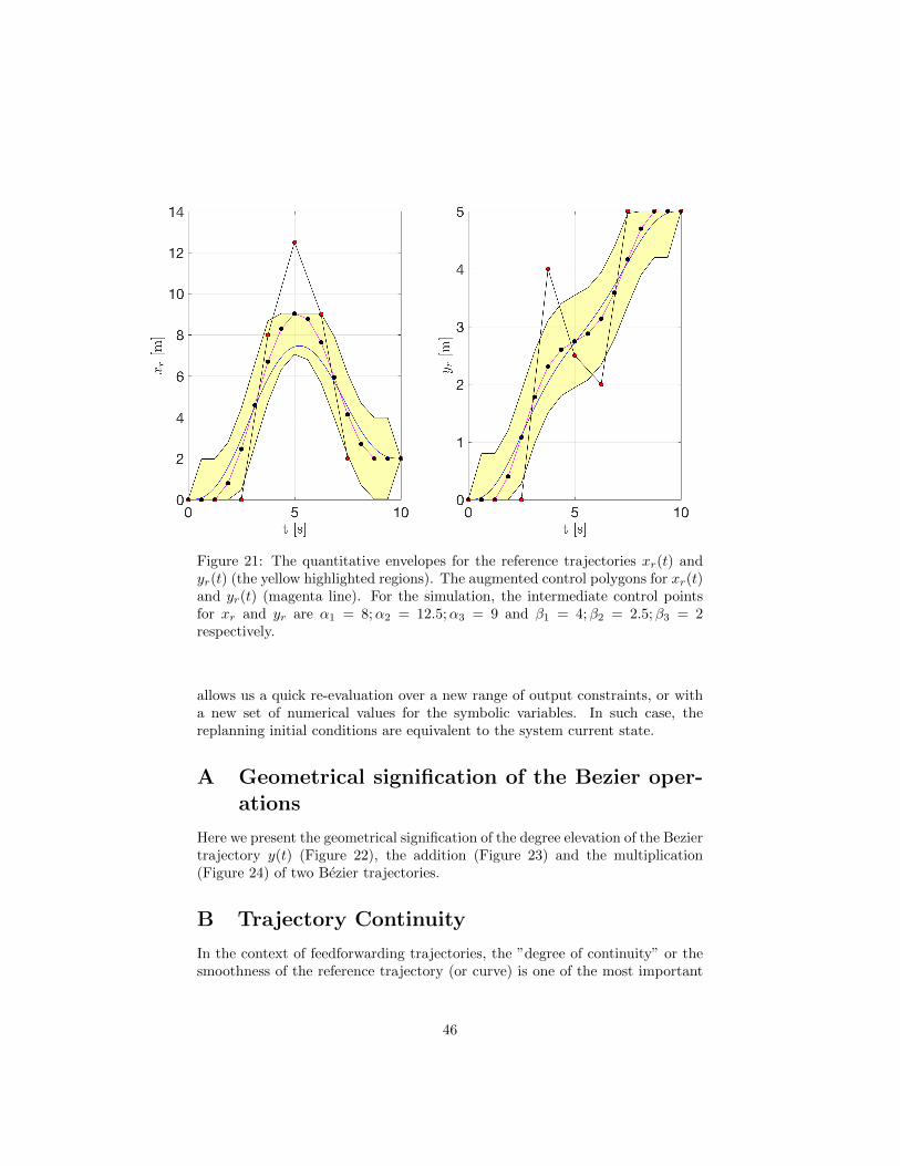
Figure 21: The quantitative envelopes for the reference trajectories xr(t) andyr(t) (the yellow highlighted regions). The augmented control polygons for xr(t)and yr(t) (magenta line). For the simulation, the intermediate control pointsfor xr and yr are α1 = 8;α2 = 12.5;α3 = 9 and β1 = 4;β2 = 2.5;β3 = 2respectively.

allows us a quick re-evaluation over a new range of output constraints, or witha new set of numerical values for the symbolic variables. In such case, thereplanning initial conditions are equivalent to the system current state.

A Geometrical signification of the Bezier oper-ations

Here we present the geometrical signification of the degree elevation of the Beziertrajectory y(t) (Figure 22), the addition (Figure 23) and the multiplication(Figure 24) of two Bezier trajectories.

B Trajectory Continuity

In the context of feedforwarding trajectories, the ”degree of continuity” or thesmoothness of the reference trajectory (or curve) is one of the most important

46

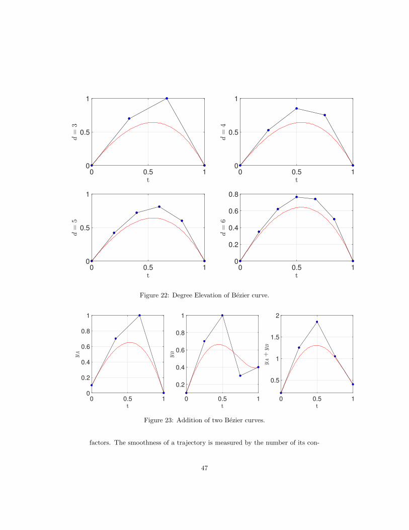
0 0.5 10

0.5

1

0 0.5 10

0.5

1

0 0.5 10

0.5

1

0 0.5 10

0.2

0.4

0.6

0.8

Figure 22: Degree Elevation of Bezier curve.

0 0.5 10

0.2

0.4

0.6

0.8

1

0 0.5 1

0.2

0.4

0.6

0.8

1

0 0.5 1

0.5

1

1.5

2

Figure 23: Addition of two Bezier curves.

factors. The smoothness of a trajectory is measured by the number of its con-

47

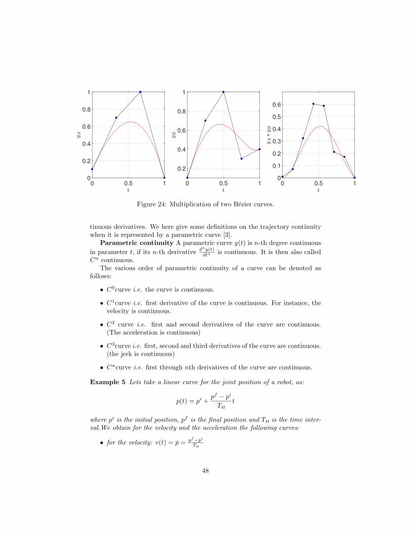
0 0.5 10

0.2

0.4

0.6

0.8

1

0 0.5 1

0.2

0.4

0.6

0.8

1

0 0.5 10

0.1

0.2

0.3

0.4

0.5

0.6

Figure 24: Multiplication of two Bezier curves.

tinuous derivatives. We here give some definitions on the trajectory continuitywhen it is represented by a parametric curve [3].

Parametric continuity A parametric curve y(t) is n-th degree continuous

in parameter t, if its n-th derivative dny(t)dtn is continuous. It is then also called

Cn continuous.The various order of parametric continuity of a curve can be denoted as

follows:

• C0curve i.e. the curve is continuous.

• C1curve i.e. first derivative of the curve is continuous. For instance, thevelocity is continuous.

• C2 curve i.e. first and second derivatives of the curve are continuous.(The acceleration is continuous)

• C3curve i.e. first, second and third derivatives of the curve are continuous.(the jerk is continuous)

• Cncurve i.e. first through nth derivatives of the curve are continuous.

Example 5 Lets take a linear curve for the joint position of a robot, as:

p(t) = pi +pf − pi

Tttt

where pi is the initial position, pf is the final position and Ttt is the time inter-val.We obtain for the velocity and the acceleration the following curves:

• for the velocity: v(t) = p = pf−piTtt

48

• for the acceleration a(t) = p =

{∞, t = 0, Ttt

0, 0 < t < Ttt

In this example, we can observe infinite accelerations at endpoints and discon-tinuous velocity when two trajectory segments are connected.

References

[1] Hirokazu Anai. Effective quantifier elimination for industrial applications.In ISSAC, pages 18–19, 2014.

[2] Martin Bak. Control of Systems with Constraints. PhD thesis, 2000.

[3] Brian A. Barsky and Tony D. DeRose. Geometric Continuity of Para-metric Curves: Constructions of Geometrically Continuous Splines. IEEEComputer Graphics and Applications, 10(1):60–68, 1990.

[4] Saugata Basu. Algorithms in real algebraic geometry: a survey. arXivpreprint arXiv:1409.1534, 2014.

[5] Christopher W Brown. An overview of QEPCAD B: a tool for real quan-tifier elimination and formula simplification. Journal of Japan Society forSymbolic and Algebraic Computation, 10(1):13–22, 2003.

[6] Ning Cao and Alan F. Lynch. Inner-Outer Loop Control for QuadrotorUAVs with Input and State Constraints. IEEE Transactions on ControlSystems Technology, 24(5):1797–1804, 2016.

[7] Garcia Carlos E., Prett David M., and Morari Manfred. Model PredictiveControl : Theory and Practice a Survey. Automatica, 25(3):335–338, 1989.

[8] Abbas Chamseddine, Youmin Zhang, Camille Alain Rabbath, Cedric Join,and Didier Theilliol. Flatness-based trajectory planning/replanning for aquadrotor unmanned aerial vehicle. IEEE Transactions on Aerospace andElectronic Systems, 48(4):2832–2847, 2012.

[9] Abbas Chamseddine, Youmin Zhang, Camille Alain Rabbath, and DidierTheilliol. Trajectory Planning and Replanning Strategies Applied to aQuadrotor Unmanned Aerial Vehicle. Journal of Guidance, Control, andDynamics, 35(5):1667–1671, 2012.

[10] George E Collins. Quantifier elimination for real closed fields by cylindricalalgebraic decompostion. In Automata Theory and Formal Languages 2ndGI Conference Kaiserslautern, May 20–23, 1975, pages 134–183. Springer,1975.

[11] Michel Coste. An introduction to semialgebraic geometry. Universite deRennes, 2002.

49

[12] Fabrizio Dabbene, Didier Henrion, and Constantino M. Lagoa. Simpleapproximations of semialgebraic sets and their applications to control. Au-tomatica, 78:110–118, 2017.

[13] Carl de Boor. A Practical Guide to Splines, volume 27. Springer, NewYork, 2001.

[14] Rida T Farouki and V. T. Rajan. Algorithms for polynomials in Bernsteinform. Computer Aided Geometric Design, 5(1):1–26, 1988.

[15] Matthias Fassler. Quadrotor Control for Accurate Agile Flight. PhD thesis,University of Zurich, 2018.

[16] Timm Faulwasser, Veit Hagenmeyer, and Rolf Findeisen. Optimal exactpath-following for constrained differentially flat systems. IFAC ProceedingsVolumes (IFAC-PapersOnline), 18(PART 1):9875–9880, 2011.

[17] Timm Faulwasser, Veit Hagenmeyer, and Rolf Findeisen. Constrainedreachability and trajectory generation for flat systems. Automatica,50(4):1151–1159, 2014.

[18] Michel Fliess. Generalized controller canonical form for linear and nonlineardynamics. IEEE Transactions on Automatic Control, 35(9):994–1001, 1990.

[19] Michel Fliess, Jean Levine, Philippe Martin, and Pierre Rouchon. A lie-backlund approach to equivalence and flatness of nonlinear systems. IEEETransactions on Automatic Control, 44(5):922–937, 1999.

[20] Michel Fliess, Jean Levine, Phillipe Martin, and Pierre Rouchon. Flat-ness and defect of non-linear systems: introductory theory and examples.International Journal of Control, 61(6):1327–1361, 1995.

[21] Melvin E. Flores and Mark B. Milam. Trajectory generation for differ-entially flat systems via NURBS basis functions with obstacle avoidance.Proceedings of the American Control Conference, 2006:5769–5775, 2006.

[22] Alessandro Gasparetto and Vanni Zanotto. A technique for time-jerk op-timal planning of robot trajectories. Robotics and Computer-IntegratedManufacturing, 24(3):415–426, 2008.

[23] Knut Graichen and Michael Zeitz. Feedforward Control Design for Finite-Time Transition Problems of Nonlinear Systems With Input and OutputConstraints. IEEE Transactions on Automatic Control, 53(5):485–488,2008.

[24] Veit Hagenmeyer. Robust nonlinear tracking control based on differen-tial flatness. at-Automatisierungstechnik Methoden und Anwendungen derSteuerungs-, Regelungs-und Informationstechnik, 50(12/2002):615, 2002.

50

[25] Veit Hagenmeyer and Emmanuel Delaleau. Exact feedforward linearizationbased on differential flatness. International Journal of Control, 76(6):537–556, 2003.

[26] Veit Hagenmeyer and Emmanuel Delaleau. Continuous-time non-linearflatness-based predictive control: an exact feedforward linearisation set-ting with an induction drive example. International Journal of Control,81(10):1645–1663, 2008.

[27] Veit Hagenmeyer and Emmanuel Delaleau. Robustness analysis with re-spect to exogenous pertubations for flatness-based exact feedforward lin-earization. IEEE Transactions on Automatic Control, 55(3):727–731, 2010.

[28] Manuel Kauers. How to use cylindrical algebraic decomposition. SeminaireLothraringien, 65(2011):1–16, 2011.

[29] Steven M LaValle. Planning algorithms. Cambridge university press, 2006.

[30] Stephen R Lindemann and Steven M Lavalle. Computing Smooth FeedbackPlans Over Cylindrical Algebraic Decompositions. In Robotics:Science andSystems, Philadelphia, USA, 2006.

[31] W. Van Loock, Goele Pipeleers, and Jan Swevers. B-spline parameterizedoptimal motion trajectories for robotic systems with guaranteed constraintsatisfaction. Mechanical Sciences, 6(2):163–171, 2015.

[32] David Lutterkort. Envelopes of Nonlinear Geometry. PhD thesis, PurdueUniversity, 1999.

[33] Tom Lyche and Knut Morken. Spline Methods. 2002.

[34] Victor Magron, Didier Henrion, and Jean-Bernard Lasserre. Semidefiniteapproximations of projections and polynomial images of semialgebraic sets.SIAM Journal on Optimization, 25(4):2143–2164, 2015.

[35] Philipp Mai, Cedric Join, and Johan Reger. Flatness-based fault tolerantcontrol of a nonlinear MIMO system using algebraic derivative estimationTo cite this version :. In 3rd IFAC Symposium on System, Structure andControl, 2007.

[36] Philippe Martin, Pierre Rouchon, and Richard M. Murray. Flat systems,equivalence and trajectory generation. 3rd cycle. edition, 2006.

[37] David Q. Mayne, J. B. Rawlings, C. V. Rao, and P. O.M. Scokaert. Con-strained model predictive control: Stability and optimality. Automatica,36(6):789–814, 2000.

[38] Daniel Mellinger and Vijay Kumar. Minimum snap trajectory generationand control for quadrotors. Proceedings - IEEE International Conferenceon Robotics and Automation, pages 2520–2525, 2011.

51

[39] Knut Mørken. Some identities for products and degree raising of splines.Constructive Approximation, 7(1):195–208, 1991.

[40] David Nairn, Jorg Peters, and David Lutterkort. Sharp , quantitativebounds on the distance between a polynomial piece and its Bezier controlpolygon. Computer Aided Geometric Design, 16:613–631, 1999.

[41] Hartmut Prautzsch, Wolfgang Boehm, and Marco Paluszny. Bezier andB-spline techniques. Springer Science & Business Media, 2002.

[42] Mohammadreza Radmanesh and Manish Kumar. Flight formation of UAVsin presence of moving obstacles using fast-dynamic mixed integer linearprogramming. Aerospace Science and Technology, 50(December):149–160,2016.

[43] Stefan Ratschan. Applications of Quantified Constraint Solving over theReals Bibliography. ArXiv, pages 1–13, 2012.

[44] Hebertt Sira-Ramirez. On the linear control of the quad-rotor system. InProceedings of the 2011 American Control Conference, pages 3178–3183,2011.

[45] Hebertt Sira-Ramirez and Sunil K Agrawal. Differentially flat systems.CRC Press, 2004.

[46] Adam W. Strzebonski. Cylindrical Algebraic Decomposition using vali-dated numerics. Journal of Symbolic Computation, 41(9):1021–1038, 2006.

[47] Fajar Suryawan, Jose De Dona, and Maria Seron. Splines and polynomialtools for flatness-based constrained motion planning. International Journalof Systems Science, 43(8):1396–1411, 2012.

[48] Alfred Tarski. A decision method for elementary algebra and geometry. InQuantifier elimination and cylindrical algebraic decomposition, pages 24–84. Springer, 1998.

[49] Didier Theilliol, Cedric Join, Youmin Zhang, Didier Theilliol, Cedric Join,and Youmin Zhang. Actuator fault-tolerant control design based on recon-figurable reference input. International Journal of Applied Mathematicsand Computer Science, De Gruyter, 18(4):553–560, 2008.

[50] Jorge Villagra, Brigitte D Andrea-novel, Michel Fliess, Hugues Mounier,Jorge Villagra, Brigitte D Andrea-novel, Michel Fliess, Hugues MounierRobust, Jorge Villagra, Brigitte Andr, Michel Fliess, and Hugues Mounier.Robust grey-box closed-loop stop-and-go control To cite this version : HALId : inria-00319591 Robust grey-box closed-loop stop-and-go control. 2008.

[51] Johannes von Lowis and Joachim Rudolph. Real-time trajectory generationfor flat systems with constraints. In Nonlinear and Adaptive Control, pages385–394. 2002.

52

[52] David J. Wilson, Russell J. Bradford, James H. Davenport, and MatthewEngland. Cylindrical Algebraic Sub-Decompositions. Mathematics in Com-puter Science, 8(2):263–288, 2014.

[53] Jing Yu, Zhihao Cai, and Yingxun Wang. Minimum jerk trajectory gen-eration of a quadrotor based on the differential flatness. In Proceedings of2014 IEEE Chinese Guidance, Navigation and Control Conference, pages832–837. IEEE, 2014.

53