Ph.d. coursein“Advancedstatistical ...publicifsv.sund.ku.dk/~pka/avepi18/day2-18.pdf · 2 ˘˜2 1...
66
Ph.d. course in “Advanced statistical analysis of epidemiological studies” Interaction Dose-response models www.biostat.ku.dk/~pka/avepi18 Clayton & Hills, Ch. 24-26 2 November 2018 Per Kragh Andersen 1
Transcript of Ph.d. coursein“Advancedstatistical ...publicifsv.sund.ku.dk/~pka/avepi18/day2-18.pdf · 2 ˘˜2 1...
Ph.d. course in “Advanced statisticalanalysis of epidemiological studies”
Interaction
Dose-response models
www.biostat.ku.dk/~pka/avepi18
Clayton & Hills, Ch. 24-26
2 November 2018
Per Kragh Andersen
1

Hypothesis tests, ch. 24Wald test for a single parameter:
W =
(M − 0
S
)2
∼ χ21 (chi-square)
directly based on computer output:
Table 24.1. Program output for the diet data.
Parameter Estimate, M SD, S W
Corner -5.4180 0.4420
Exposure (1) 0.8697 0.3080 7.97
Age (1) 0.1290 0.4753 0.07
Age (2) 0.6920 0.4614 2.25
2

Likelihood ratio test: compare max. log likelihoods “under” and“outside” the hypothesis.
Test statistic = -2 × difference between max. log likelihoods
Model Max. log likelihood # parameters
Corner + Age + Exposure -247.03 4
Corner + Exposure -249.04 2
Corner + Age -251.18 3
# parameters removed = # d.f. in χ2
Exposure: 8.30, 1 d.f.
Age: 4.02, 2 d.f.
Models have to be ”nested” - we cannot compare the last two modelsin the table.
3

Max. log likelihood: measure of goodness of fit of a model:
larger log likelihood =⇒ better fit
Interpretation of –247.03 ? No!
Some times, the deviance is introduced as a supplement to the max.log likelihood.
4

Interaction, sect. 24.3We have assumed that the effect of exposure is constant over agebands (and vice versa).
Is that reasonable?
Or is there interaction between age and exposure?
log(Rate)=Corner + Exposure + Age + Exposure·Age
Introducing interaction terms into the regression model, we:
• get a quantification of heterogeneity
• are able to adjust for other explanatory variables when examininginteraction
5
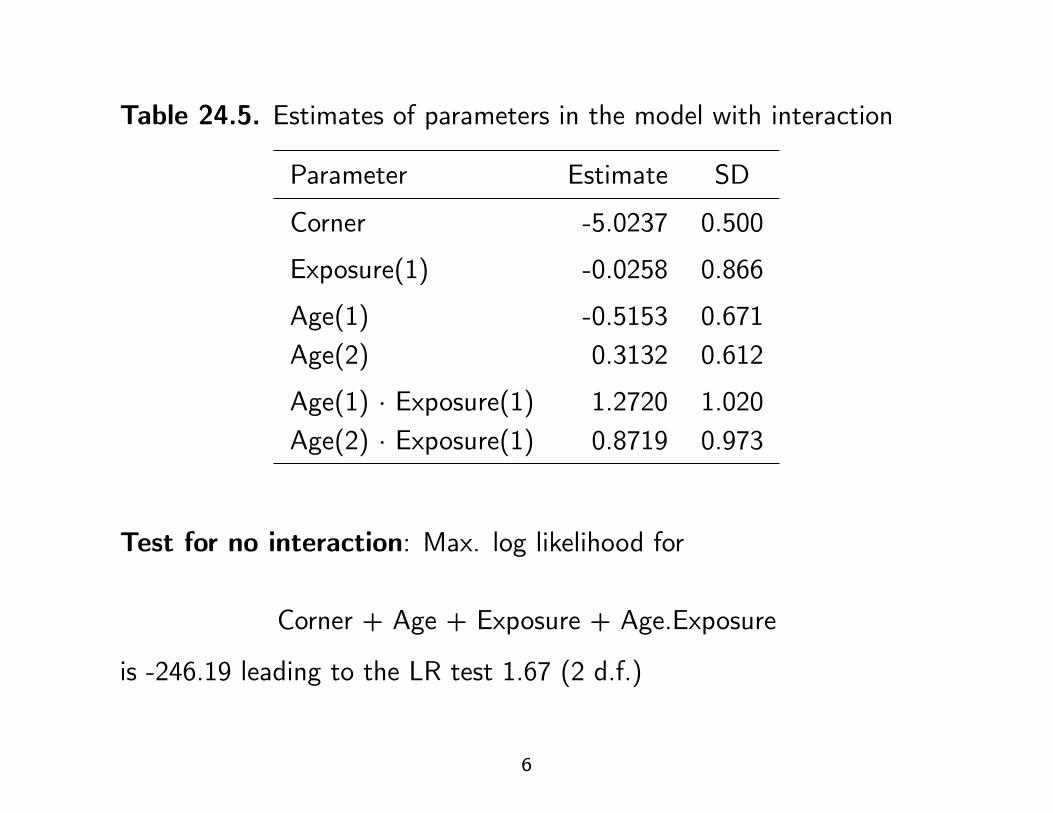
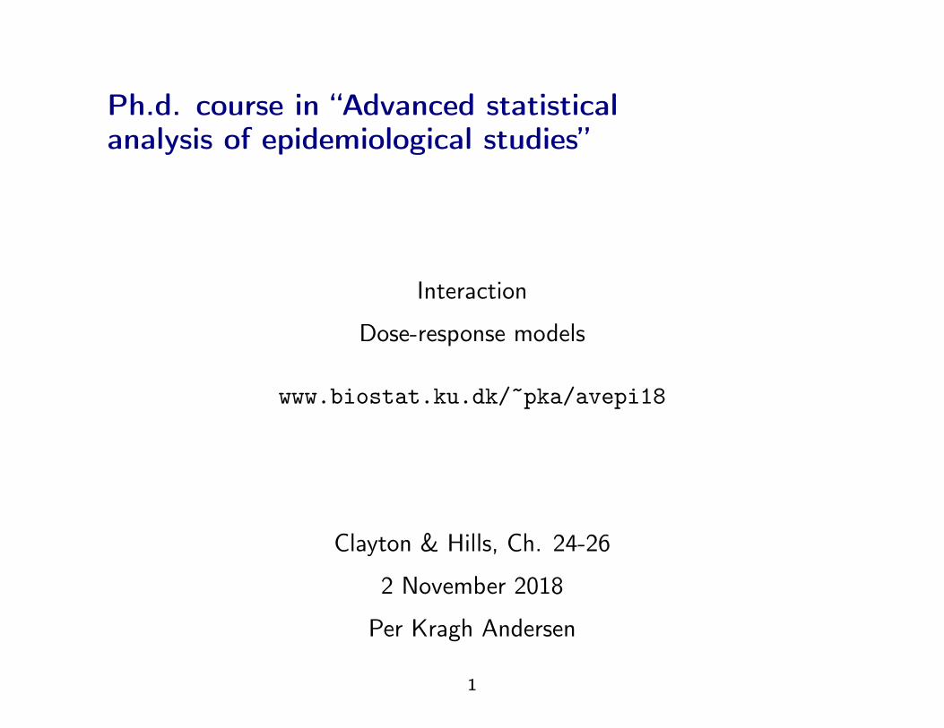
Table 24.5. Estimates of parameters in the model with interaction
Parameter Estimate SD
Corner -5.0237 0.500
Exposure(1) -0.0258 0.866
Age(1) -0.5153 0.671Age(2) 0.3132 0.612
Age(1) · Exposure(1) 1.2720 1.020Age(2) · Exposure(1) 0.8719 0.973
Test for no interaction: Max. log likelihood for
Corner + Age + Exposure + Age.Exposure
is -246.19 leading to the LR test 1.67 (2 d.f.)
6

Illustrative example without interaction Table 22.4
Exposure
Age 0 10 5.0 15.01 12.0 36.02 30.0 90.0
0 5.0 5.0 × 3.01 12.0 12.0 × 3.02 30.0 30.0 × 3.0
0 5.0 5.0 × 3.01 5.0 × 2.4 5.0 × 2.4 × 3.02 5.0 × 6.0 5.0 × 6.0 × 3.0
Corner = 5.0 Age(1) = 2.4
Exposure (1) = 3.0 Age(2) = 6.0
7

Example: Illustrative values of rates with interactionTable 24.2. Definition of interactions in terms of exposure
Exposure
Age 0 10 5.0 15.01 12.0 42.02 30.0 135.0
0 5.0 5.0 × 3.01 12.0 12.0 × 3.52 30.0 30.0 × 4.5
0 5.0 5.0 × 3.01 12.0 12.0 × 3.0 × 1.1672 30.0 30.0 × 3.0 × 1.5
interactionparameters
8

Example: Illustrative values of rates with interactionTable 24.3. Definition of interactions in terms of age
Exposure
Age 0 10 5.0 15.01 12.0 42.02 30.0 135.0
0 5.0 15.01 5.0 × 2.4 15.0 × 2.82 5.0 × 6.0 15.0 × 9.0
0 5.0 15.01 5.0 × 2.4 15.0 × 2.4 × 1.1672 5.0 × 6.0 15.0 × 6.0 × 1.5
interactionparameters
9

Table 24.4. Definition of interactions in terms of exposure and age
Exposure
Age 0 10 5.0 5.0 × 3.01 5.0 × 2.4 5.0 × 3.0 × 2.4 × 1.1672 5.0 × 6.0 5.0 × 3.0 × 6.0 × 1.5
Exercise 24.4.
10

Exercise 24.4: solution
Parameter Estimate SD
Corner -5.0237 0.500
Exposure(1) -0.0258 0.866
Age(1) -0.5153 0.671Age(2) 0.3132 0.612
Age(1) · Exposure(1) 1.2720 1.020Age(2) · Exposure(1) 0.8719 0.973
log4
607.9= −5.0237, log
2311.9
4607.9
= −0.0258
(except for rounding errors)
11

SAS programdata ihd;
input eksp alder pyrs cases;
lpyrs=log(pyrs);
datalines; /* or, alternatively, read from www */
0 2 311.9 2
0 1 878.1 12
0 0 667.5 14
1 2 607.9 4
1 1 1272.1 5
1 0 888.9 8
;
run;
proc genmod data=ihd;
class eksp alder;
model cases=eksp alder eksp*alder/dist=poi offset=lpyrs type3;
run;
12

The GENMOD Procedure
Model Information
Data Set WORK.IHD
Distribution Poisson
Link Function Log
Dependent Variable cases
Offset Variable lpyrs
Observations Used 6
Class Level Information
Class Levels Values
eksp 2 0 1
alder 3 0 1 2
13

Criteria For Assessing Goodness Of Fit
Criterion DF Value Value/DF
Deviance 0 0.0000 .
Scaled Deviance 0 0.0000 .
Pearson Chi-Square 0 0.0000 .
Scaled Pearson X2 0 0.0000 .
Log Likelihood 53.3799
14

Analysis Of Parameter Estimates
Standard Wald 95% Chi-
Parameter DF Estimate Error Confidence Limits Square
Intercept 1 -5.0237 0.5000 -6.0037 -4.0437 100.95
eksp 0 1 -0.0258 0.8660 -1.7232 1.6716 0.00
eksp 1 0 0.0000 0.0000 0.0000 0.0000 .
alder 0 1 0.3132 0.6124 -0.8871 1.5134 0.26
alder 1 1 -0.5153 0.6708 -1.8301 0.7995 0.59
alder 2 0 0.0000 0.0000 0.0000 0.0000 .
eksp*alder 0 0 1 0.8719 0.9728 -1.0349 2.7786 0.80
eksp*alder 0 1 1 1.2720 1.0165 -0.7204 3.2643 1.57
15

Analysis Of Parameter
Estimates
Parameter Pr > ChiSq
Intercept <.0001
eksp 0 0.9762
eksp 1 .
alder 0 0.6091
alder 1 0.4424
alder 2 .
eksp*alder 0 0 0.3701
eksp*alder 0 1 0.2108
16

LR Statistics For Type 3 Analysis
Chi-
Source DF Square Pr > ChiSq
eksp 1 3.09 0.0790
alder 2 4.37 0.1125
eksp*alder 2 1.67 0.4333
17

Table 24.5. Reporting estimates from the model with interaction:
Reparametrize into separate effects of Exposure within each Age band.
Parameter Estimate SD RR
Corner -5.0237 0.500
Exposure(1)·Age(0) -0.0258 0.866 0.97
Exposure(1)·Age(1) 1.2461 0.532 3.48
Exposure(1)·Age(2) 0.8461 0.443 2.33
Age(1) -0.5153 0.671 0.60Age(2) 0.3132 0.612 1.37
18
Interactions: which to study?When the model contains p covariates there are p(p− 1)/2 possibletwo-factor interactions (e.g., 45 for p = 10).
It is out of the question to study them all, so a generalrecommendation is to restrict attention to those that werepre-specified in the research protocol:
“Don’t ask a question if you are not interested in the reply!”
There will also be a type I error problem: “if you ask too manyquestions you will get too many wrong answers”.
19

Interaction is scale dependent.Table of disease rates:
Factor A Factor B
Absent Present
Absent 0.1 0.2
Present 0.3 λ
If λ = 0.6 then the rate ratio associated with the presence of factor Ais 3 both when factor B is absent or present; and the rate ratioassociated with the presence of factor B is 2 both when factor A isabsent or present.
However, the rate difference associated with the presence of factor Ais 0.2 when factor B is absent and 0.4 if it is present and the ratedifference associated with the presence of factor B is 0.1 when factorA is absent and 0.3 if it is present
20

Factor A Factor B
Absent Present
Absent 0.1 0.2
Present 0.3 λ
If λ = 0.4 then the rate difference associated with the presence offactor A is 0.2 both when factor B is absent or present; the ratedifference associated with the presence of factor B is 0.1 both whenfactor A is absent or present.
However, the rate ratio associated with the presence of factor A is 3when factor B is absent and 2 if it is present and the rate ratioassociated with the presence of factor B is 2 when factor A is absentand 1.33 if it is present
More on additive models for rates later.
21

Example: case-control study of oral cancer
Table 24.6. Cases (controls) for oral cancer study.
Alcohol (oz/day, 1 drink ∼ 0.3 oz/day).
Tobacco 0 1 2 3
(cigs/day) 0 0.1-0.3 0.4-1.5 1.6+
0 (0) 10 (38) 7 (27) 4 (12) 5 (8)
1 (1-19) 11 (26) 16 (35) 18 (16) 21 (20)
2 (20-39) 13 (36) 50 (60) 60 (49) 125 (52)
3 (40+) 9 (8) 16 (19) 27 (14) 91 (27)
Table 24.7. Case/control ratios for the oral cancer data.
Alcohol
Tobacco 0 1 2 3
0 0.26 0.26 0.33 0.63
1 0.42 0.46 1.13 1.05
2 0.36 0.83 1.22 2.40
3 1.12 0.84 1.93 3.37
22

Is the effect of tobacco the same for all levels of alcohol consumption?
= INTERACTION
(∼ SYNERGY?)
But CORRELATION is something completely different
23

Fig. 24.2. Nesting of models.
5. Corner+Alcohol+Tobacco+Alcohol.Tobacco
4. Corner+Alcohol+Tobacco
2. Corner+Alcohol 3. Corner+Tobacco
1. Corner
HHHHHj
HHHHHj
������
������
?
Exercise 24.6
24

Exercise 24.6: Log-likelihoods
5. -577.65
4. -580.99
2. -596.62 3. -608.59
1. -643.93
HHHHHj
HHHHHj
������
������
?
25
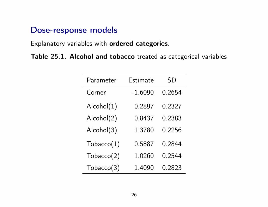
Dose-response modelsExplanatory variables with ordered categories.
Table 25.1. Alcohol and tobacco treated as categorical variables
Parameter Estimate SD
Corner -1.6090 0.2654
Alcohol(1) 0.2897 0.2327
Alcohol(2) 0.8437 0.2383
Alcohol(3) 1.3780 0.2256
Tobacco(1) 0.5887 0.2844
Tobacco(2) 1.0260 0.2544
Tobacco(3) 1.4090 0.2823
26

Alternative: monotone effect of tobaccoFig. 20.1. Log-linear trend
-
6Log(odds)
q q q q0 1 2 3 Dose, z
rr
r
###########
β
β
27

Look at successive differences between effects:
Tobacco(1), Tobacco(2)-Tobacco(1), Tobacco(3)-Tobacco(2)
Exercise 25.1
Introduce a variable
taking values 0, 1, 2 or 3 and denote its effect by
[Tobacco]
Model: log(Odds) = Corner + Alcohol + [Tobacco]
28

Exercise 25.1: solution.Table 25.1. Alcohol and tobacco treated as categorical variables
Parameter Estimate SD Succ. diff.
Corner -1.6090 0.2654
Alcohol(1) 0.2897 0.2327 0.2897
Alcohol(2) 0.8437 0.2383 0.5540
Alcohol(3) 1.3780 0.2256 0.5543
Tobacco(1) 0.5887 0.2844 0.5887
Tobacco(2) 1.0260 0.2544 0.4373
Tobacco(3) 1.4090 0.2823 0.3830
29

Model: log(Odds) = Corner + Alcohol + [Tobacco]Table 25.2. The linear effect of tobacco consumption
Alcohol Tobacco log(Odds)=Corner + ...
0 0 -
0 1 1×[Tobacco]
0 2 2×[Tobacco]
0 3 3×[Tobacco]
1 0 Alcohol(1)
1 1 Alcohol(1)+1×[Tobacco]
1 2 Alcohol(1)+2×[Tobacco]
1 3 Alcohol(1)+3×[Tobacco]
2 0 Alcohol(2)
2 1 Alcohol(2)+1×[Tobacco]
2 2 Alcohol(2)+2×[Tobacco]
2 3 Alcohol(2)+3×[Tobacco]
3 0 Alcohol(3)
3 1 Alcohol(3)+1×[Tobacco]
3 2 Alcohol(3)+2×[Tobacco]
3 3 Alcohol(3)+3×[Tobacco]
30

Table 25.3. Linear effect of tobacco per level
Parameter Estimate SD
Corner –1.5250 0.219
Alcohol(1) 0.3020 0.232
Alcohol(2) 0.8579 0.237
Alcohol(3) 1.3880 0.225
[Tobacco] 0.4541 0.083
31

Similarly with alcohol consumption:introduce variable with values=0, 1, 2 or 3and denote its effect [Alcohol]
Table 25.4. Linear effects of alcohol and tobacco per level
Parameter Estimate SD
Corner –1.6290 0.1860
[Alcohol] 0.4901 0.0676
[Tobacco] 0.4517 0.0833
Exercise 25.3
32

Exercise 25.3: solution.Tobacco(3)+Alcohol(3)=2.7870
3× [Tobacco] + 3× [Alcohol] = 2.8254
33

Alternative ways of scoringTobacco: cigarettes/day (0 : 0, 1-19 : 10, 20-39 : 30, 40+ : 50)
Alcohol: ounces/day (0.0 : 0, 0.1-0.3 : 0.2, 0.4-1.5 : 1.0, 1.6+ : 2.0)
Table 25.5. Alcohol in ounces/day and tobacco in cigarettes/day
Parameter Estimate SD
Corner –1.2657 0.1539
[Alcohol] 0.6484 0.0881
[Tobacco] 0.0253 0.0046
34

Testing
– Test for linearity:
1) Comparing the “nested” models:log(Odds) = Corner + Alcohol + Tobacco
andlog(Odds) = Corner + Alcohol + [Tobacco],
here: LR test=0.38, 2. d.f.,
or
2) eliminating [Tobsq] (=0, 1, 4, 9) fromlog(Odds) = Corner + Alcohol + [Tobacco] + [Tobsq],
here LR test=0.02.
35

– Trend test: (1. d.f.) Eliminating [Tobacco] from the model:log(Odds) = Corner + Alcohol + [Tobacco],
here LR test=30.88.
Why not use individual levels, that is, a truly quantitative covariateand no categorization at all?
Pros and cons
• Information is lost by categorization
• Categories may be more robust (e.g., smoking)
• Few outliers may have large influence (“Casanova effect”!)
• Model with a linear effect is no longer “nested” in categoricalmodel ⇒ alternative alternatives are needed when testing linearity
36

Indicator (‘dummy’) variablesThe way in which the categorical covariates are entered into theregression model.
Table 25.8. Indicator variables for the three alcohol parameters
A1 A2 A3 Level log(Odds) = Corner + · · ·
0 0 0 0 –
1 0 0 1 Alcohol(1)
0 1 0 2 Alcohol(2)
0 0 1 3 Alcohol(3)
37

The use of indicator variables enables the programmer to choosehis/her preferred reference level.
Interaction terms are simple products of indicator variabels.
Table 25.10. Indicator variables for interaction parameters
A1 A2 A3 T A1 · T A2 · T A3 · T
0 0 0 0 0 0 00 0 0 1 0 0 01 0 0 0 0 0 01 0 0 1 1 0 00 1 0 0 0 0 00 1 0 1 0 1 00 0 1 0 0 0 00 0 1 1 0 0 1
NB: Tobacco is here on 2 levels only
38

Treating the zero level differentlyFig. 25.1. Separating zero exposure from the dose-response.
-
6Log(odds)
q q q q0 1 2 3 Dose, z
rr r r
CornerCorner+Non-smoker
Non-smoker
""""""""
%%%%"""
39

Corresponds to adding a new variable [Non-smoker]
Table 25.11. Separating zero exposure from the dose-response
Tobacco Non-smoker log(Odds) = Corner + · · ·
0 1 [Non-smoker]
1 0 1 × [Tobacco]
2 0 2 × [Tobacco]
3 0 3 × [Tobacco]
(Alternative: include [Smoker] = 1 - [Non-smoker])
40

Indicator variables may be chosen in several ways.
E.g., to model successive differences
Table 25.12. Indicators to compare each level with the one before
Tobacco D1 D2 D3
0 0 0 01 1 0 02 1 1 03 1 1 1
Here, D1 = indicator for Tobacco ≥ 1
D2 = indicator for Tobacco ≥ 2
D3 = indicator for Tobacco ≥ 3
41

data oral;
filename oraldata
url ’http://publicifsv.sund.ku.dk/~pka/epidata/oral.txt’;
infile oraldata firstobs=2;
input cases controls alc tob;
total=cases+controls;
run;
proc genmod data=oral;
class tob (ref=’0’) alc (ref=’0’);
model cases/total=tob alc/dist=binomial type3;
run;
42

/* ***** NEW DATA STEP IN SAME SAS PROGRAM ***** */
data oral; set oral;
tob0=(tob=0); tob1=(tob=1);
tob2=(tob=2); tob3=(tob=3);
alc0=(alc=0); alc1=(alc=1);
alc2=(alc=2); alc3=(alc=3);
run;
/* ***** FURTHER PROCedure STEPS ***** */
proc genmod data=oral;
model cases/total=tob alc1 alc2 alc3/dist=binomial type3;
run;
proc genmod data=oral;
model cases/total=tob alc0 alc1 alc2/dist=binomial type3;
run;
proc genmod data=oral;
model cases/total=tob tob0 alc0 alc1 alc2/dist=binomial type3;
run;
43
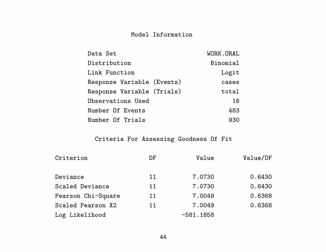
Model Information
Data Set WORK.ORAL
Distribution Binomial
Link Function Logit
Response Variable (Events) cases
Response Variable (Trials) total
Observations Used 16
Number Of Events 483
Number Of Trials 930
Criteria For Assessing Goodness Of Fit
Criterion DF Value Value/DF
Deviance 11 7.0730 0.6430
Scaled Deviance 11 7.0730 0.6430
Pearson Chi-Square 11 7.0049 0.6368
Scaled Pearson X2 11 7.0049 0.6368
Log Likelihood -581.1858
44

Analysis Of Parameter Estimates
Standard Wald 95% Confidence Chi-
Parameter DF Estimate Error Limits Square
Intercept 1 -1.5252 0.2193 -1.9551 -1.0954 48.37
tob 1 0.4541 0.0834 0.2907 0.6175 29.67
alc1 1 0.3020 0.2316 -0.1519 0.7558 1.70
alc2 1 0.8579 0.2369 0.3935 1.3223 13.11
alc3 1 1.3880 0.2249 0.9472 1.8288 38.09
Scale 0 1.0000 0.0000 1.0000 1.0000
Parameter Pr > ChiSq
Intercept <.0001
tob <.0001
alc1 0.1922
alc2 0.0003
alc3 <.0001
45
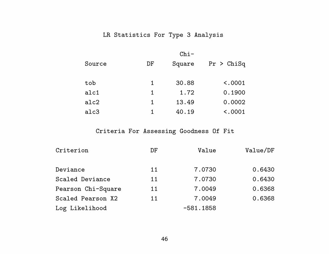
LR Statistics For Type 3 Analysis
Chi-
Source DF Square Pr > ChiSq
tob 1 30.88 <.0001
alc1 1 1.72 0.1900
alc2 1 13.49 0.0002
alc3 1 40.19 <.0001
Criteria For Assessing Goodness Of Fit
Criterion DF Value Value/DF
Deviance 11 7.0730 0.6430
Scaled Deviance 11 7.0730 0.6430
Pearson Chi-Square 11 7.0049 0.6368
Scaled Pearson X2 11 7.0049 0.6368
Log Likelihood -581.1858
46

Analysis Of Parameter Estimates
Standard Wald 95% Confidence Chi-
Parameter DF Estimate Error Limits Square
Intercept 1 -0.1373 0.2081 -0.5452 0.2706 0.44
tob 1 0.4541 0.0834 0.2907 0.6175 29.67
alc0 1 -1.3880 0.2249 -1.8288 -0.9472 38.09
alc1 1 -1.0860 0.1834 -1.4455 -0.7265 35.06
alc2 1 -0.5301 0.1870 -0.8965 -0.1636 8.04
Scale 0 1.0000 0.0000 1.0000 1.0000
Parameter Pr > ChiSq
Intercept 0.5094
tob <.0001
alc0 <.0001
alc1 <.0001
alc2 0.0046
47

LR Statistics For Type 3 Analysis
Chi-
Source DF Square Pr > ChiSq
tob 1 30.88 <.0001
alc0 1 40.19 <.0001
alc1 1 35.95 <.0001
alc2 1 8.03 0.0046
Criteria For Assessing Goodness Of Fit
Criterion DF Value Value/DF
Deviance 10 6.7227 0.6723
Scaled Deviance 10 6.7227 0.6723
Pearson Chi-Square 10 6.6852 0.6685
Scaled Pearson X2 10 6.6852 0.6685
Log Likelihood -581.0106
48
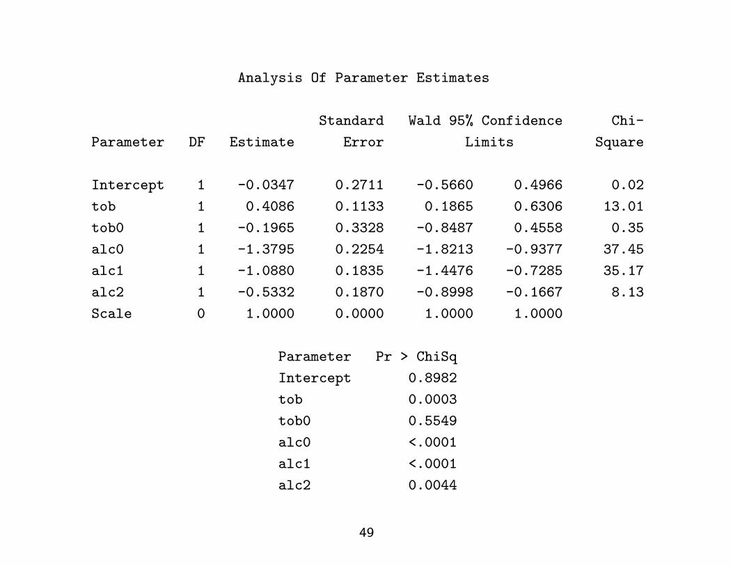
Analysis Of Parameter Estimates
Standard Wald 95% Confidence Chi-
Parameter DF Estimate Error Limits Square
Intercept 1 -0.0347 0.2711 -0.5660 0.4966 0.02
tob 1 0.4086 0.1133 0.1865 0.6306 13.01
tob0 1 -0.1965 0.3328 -0.8487 0.4558 0.35
alc0 1 -1.3795 0.2254 -1.8213 -0.9377 37.45
alc1 1 -1.0880 0.1835 -1.4476 -0.7285 35.17
alc2 1 -0.5332 0.1870 -0.8998 -0.1667 8.13
Scale 0 1.0000 0.0000 1.0000 1.0000
Parameter Pr > ChiSq
Intercept 0.8982
tob 0.0003
tob0 0.5549
alc0 <.0001
alc1 <.0001
alc2 0.0044
49

The GENMOD Procedure
LR Statistics For Type 3 Analysis
Chi-
Source DF Square Pr > ChiSq
tob 1 13.22 0.0003
tob0 1 0.35 0.5539
alc0 1 39.41 <.0001
alc1 1 36.07 <.0001
alc2 1 8.12 0.0044
50

More on quantitative covariatesIn a model like
log(Rate)=Corner + Exposure + [x]
the effect of x is assumed to be linear, i.e. [x] expresses the change inlog(Rate) per 1 unit change of x.
To test for linearity, one may add [xsq] to the model where xsq= x2.
An alternative alternative is a linear spline.
51

Linear splinesAn alternative to a straight line is a broken line.
Introduce break points for x, e.g., a1, a2, a3 and add the three linearsplines
I1 × [x− a1], I2 × [x− a2], I3 × [x− a3]
to [x]:
Here, I1 = indicator for x ≥ a1I2 = indicator for x ≥ a2I3 = indicator for x ≥ a3
The parameter for the spline I1 × [x− a1] = x+1 , say gives the changein slope at the break point a1. Similarly at a2, a3.
Splines are easy to program and parameters are easier to interpret thanfor quadratic terms.
52

SAS code for linear splines
data new; set old;
if x<a1 then spline1=0; if x>=a1 then spline1=x-a1;
if x<a2 then spline2=0; if x>=a2 then spline1=x-a2;
/* Alternatively - use dummy variables:
spline1=(x-a1)*(x>=a1); spline2=(x-a2)*(x>=a2); */
run;
53

2 4 6 8 10
−2.0
−1.5
−1.0
−0.5
0.00.5
x
Linea
r Pred
ictor
2 4 6 8 10
−2.0
−1.5
−1.0
−0.5
0.00.5
x
Linea
r Pred
ictor
2 4 6 8 10
−2.0
−1.5
−1.0
−0.5
0.00.5
x
Linea
r pred
ictor
2 4 6 8 10
−2.0
−1.5
−1.0
−0.5
0.00.5
x
Linea
r Pred
ictor
54

Quadratic and restricted splinesThe linear spline function is continuous but not smooth. The ‘linearpredictor’ is:
a+ b1xi + b1,1x+i1 + ...+ b1,3x
+i3.
Linear predictor with quadratic splines:
a+ b1xi + b2x2i + b1,1(x
+i1)
2 + ...+ b1,3(x+i3)
2.
No simple interpretation of coefficients, but a smooth curve isobtained. LR test for linearity b2 = b1,1 = ... = b1,3 = 0.
The quadratic effect b2x2i may be quite dramatic for large (bothpositive and negative) values of xi (‘Casanova’ again!).
This may be avoided using restricted splines. The idea is that for large(positive or negative) x’s, the curve is linear instead of quadratic.
Also cubic splines may be defined: (x+ij)3.
55

Additive models for ratesAdditive Poisson model for diet data:
Rate = Corner + Age + Exposure,
CasesPyrs
= Corner + Age + Exposure,
Cases = Pyrs × (Corner + Age + Exposure).
That is:
• ‘identity link’ instead of log link
• Corner replaced by Pyrs times Corner
• explanatory variables also multiplied by Pyrs
• no ‘offset’ needed
56

SAS program using indicator variablesdata ihd;
input eksp alder pyrs cases;
pyrs=pyrs/1000;
age0=pyrs*(alder=2); age1=pyrs*(alder=1); age2=pyrs*(alder=0);
eksp0=pyrs*(eksp=1); eksp1=pyrs*(eksp=0);
datalines;
0 2 311.9 2
0 1 878.1 12
0 0 667.5 14
1 2 607.9 4
1 1 1272.1 5
1 0 888.9 8
;
run;
proc genmod data=ihd;
model cases=pyrs age1 age2 eksp1/dist=poi link=id noint;
run;
57

SAS output (edited)The GENMOD Procedure
Model Information
Data Set WORK.IHD
Distribution Poisson
Link Function Identity
Dependent Variable cases
Number of Observations Read 6
Number of Observations Used 6
Criteria For Assessing Goodness Of Fit
Criterion DF Value Value/DF
Deviance 2 2.1024 1.0512
Scaled Deviance 2 2.1024 1.0512
Pearson Chi-Square 2 1.8369 0.9185
Scaled Pearson X2 2 1.8369 0.9185
Log Likelihood 52.3287
58

Analysis Of Parameter Estimates
Standard Wald 95% Confidence Chi-
Parameter DF Estimate Error Limits Square
Intercept 0 0.0000 0.0000 0.0000 0.0000 .
pyrs 1 5.1758 2.5085 0.2593 10.0924 4.26
age1 1 -1.0028 3.0344 -6.9501 4.9445 0.11
age2 1 4.8503 3.9117 -2.8164 12.5171 1.54
eksp1 1 8.4316 3.2113 2.1376 14.7255 6.89
Scale 0 1.0000 0.0000 1.0000 1.0000
Analysis Of Parameter Estimates
Parameter Pr > ChiSq
Intercept .
pyrs 0.0391
age1 0.7410
age2 0.2150
eksp1 0.0086
59

Observed and predicted ratesTable 22.6. Energy intake and IHD incidence per 1000 person-years(D = Cases, Y = P-yrs.)
Exposed Unexposed
Current (< 2750 kcal) (≥ 2750 kcal)
age D Y Rate D Y Rate RD
40–49 2 311.9 6.41 (13.61) 4 607.9 6.58 (5.18) -0.17
50–59 12 878.1 13.67 (12.61) 5 1271.1 3.93 (4.18) 9.74
60–69 14 667.5 20.97 (18.46) 8 888.9 9.00 (10.03) 11.97
60

SAS program using indicator variables: interactiondata ihd;
input eksp alder pyrs cases;
pyrs=pyrs/1000;
age0=pyrs*(alder=2); age1=pyrs*(alder=1); age2=pyrs*(alder=0);
eksp0=pyrs*(eksp=1); eksp1=pyrs*(eksp=0);
age1exp1=(alder=1)*(eksp=0)*pyrs; age2exp1=(alder=0)*(eksp=0)*pyrs;
datalines;
0 2 311.9 2
0 1 878.1 12
0 0 667.5 14
1 2 607.9 4
1 1 1272.1 5
1 0 888.9 8
;
run;
proc genmod data=ihd;
model cases=pyrs age1 age2 eksp1 age1exp1 age2exp1/dist=poi link=id noint;
run;
61

SAS output (edited)The GENMOD Procedure
Model Information
Data Set WORK.IHD
Distribution Poisson
Link Function Identity
Dependent Variable cases
Number of Observations Read 6
Number of Observations Used 6
Criteria For Assessing Goodness Of Fit
Criterion DF Value Value/DF
Deviance 0 0.0000 .
Scaled Deviance 0 0.0000 .
Pearson Chi-Square 0 0.0000 .
Scaled Pearson X2 0 0.0000 .
Log Likelihood 53.3799
62

Analysis Of Parameter Estimates
Standard Wald 95% Confidence Chi-
Parameter DF Estimate Error Limits Square
Intercept 0 0.0000 0.0000 0.0000 0.0000 .
pyrs 1 6.5800 3.2900 0.1317 13.0283 4.00
age1 1 -2.6495 3.7301 -9.9605 4.6614 0.50
age2 1 2.4199 4.5770 -6.5509 11.3906 0.28
eksp1 1 -0.1677 5.6021 -11.1476 10.8121 0.00
age1exp1 1 9.9031 7.0736 -3.9609 23.7671 1.96
age2exp1 1 12.1416 8.5399 -4.5962 28.8794 2.02
Scale 0 1.0000 0.0000 1.0000 1.0000
Parameter Pr > ChiSq
Intercept .
pyrs 0.0455
age1 0.4775
age2 0.5970
eksp1 0.9761
age1exp1 0.1615
age2exp1 0.1551
63

Exercise 1Consider the data from last time from Doll & Hill’s famous study ofsmoking and cardiovascular mortality among British doctors (see thefile doctors.txt).
1. Examine if there is an interaction between age and smoking by addingthe term smoke*agegrp to the model including smoke and agegrp.
2. In the model with interaction, drop the ‘main effect’ (smoke) andinterpret the resulting parameter estimates.
3. Examine if the effect of agegrp can be assumed to be linear.
4. Fit a model where the effect of agegrp is a linear spline. Do the test forlinearity.
5. Return to treating age and smoking as categorical variables. Fit anadditive rate model and study whether there is an interaction betweenage and smoking on the additive scale.
64

Exercise 2This exercise continues the analysis of the oral cancer example inClayton & Hills’ Table 24.6 (see the file oral.txt).
1. Fit all the models in Clayton & Hills Fig. 24.2 (slide 24) and reconstructthe likelihood ratio tests from Clayton & Hills Exercise 24.6 (slide 25).
2. Try to test for linearity for tob by defining a new variable(tobsq=tob*tob) and add it to the model where both tob and alc
enter linearly. What is the conclusion concerning linearity of tob?
3. Test for linearity when tobacco is instead coded as in C & H’s Table25.5 (slide 34). For which of the two ways of coding the variable doesthe linear model give the better fit?
4. Fit the model where tob enters linearly and alc is categorical. Whathappens if an interaction term is added? Interpret the results.
5. Fit the model where both tob and alc enter linearly. What happens ifan interaction term is added? Interpret the results.
65

Description of data set oral.txtThe data set is available from
publicifsv.sund.ku.dk/~pka/epidata
• There are 1 + 16 lines: line no. 1 contains names of variables,and there is one line for each of the cells in the four-by-four table.
• cases: number of cases
• controls: number of controls
• alc: 0, 1, 2 or 3 giving the level of alcohol consumption
• tob: 0, 1, 2 or 3 giving the level of tobacco consumption
66