I  

Master Thesis

Phase-field Modeling of

Crystal Growth

during Deformation  

 

 

 

 

 

Tan Xu

Department of Ferrous Technology

(Computational Metallurgy)

Graduate Institute of Ferrous Technology

Pohang University of Science and Technology

2010  

 

II  

Phase-field Modeling of Crystal Growth during Deformation

 

III  

Phase-field Modeling of

Crystal Growth during Deformation

 

 

by Tan Xu

Department of Ferrous Technology (Computational Metallurgy)

Graduate Institute of Ferrous Technology Pohang University of Science and Technology

  

A thesis submitted to the faculty of Pohang University of Science and Technology in partial fulfillments of the requirements for the degree of Master of Science in the Graduate Institute of Ferrous Technology Pohang, Korea 21. June. 2010 Approved by

Prof. Rongshan, Qin ___________ Prof. Bhadeshia. H.K.D.H__________

Major Advisor

IV  

Phase-filed Modeling of

Crystal Growth during Deformation

Tan Xu This dissertation is submitted for the degree of Master of

Science at the Graduate Institute of Ferrous Technology of

Pohang University of Science and Technology. The research

reported herein was approved by the committee of Thesis

Appraisal 21. June. 2010  

 

 

 

Thesis Review Committee Chairman: Barlat, Frederic _____________ Member: Kim, In Gee _____________

Member: Suh, Dong-Woo _____________  

 

V  

MFT

20081013

 

 

ABSTRACT 

 

 

 

A method to compute crystal growth during materi

als deformation has been developed. This is done b

y firstly extension of the numerical solution of the

recent developed phase-field model from regular l

attice to the irregular lattice. Accurate mathematic

s and discrete algorithms are derived for solving p

hase-field governing equation in generic spatial co

nfigurations. The homogeneous deformation is mod

eled as vector operator on each lattice. The metho

d enables the simulation of warm rolling, a thermo

mechanical processing method possessing huge po

Tan Xu

Phase-field Modeling of Crystal Growth

during Deformation

Department of Ferrous Technology

(Computational Metallurgy) 2010

Advisor: Professor Rongshan, Qin and

Professor H.K.D.H.Bhadeshia

Text in English

VI  

tential for making high quality steels but far behind

the scientific understanding due to the complex n

ature of that the phase transition and deformation t

ake place simultaneously. Numerical simulation of t

hree-dimensional crystal growth in deformation de

monstrates interesting morphological evolution, an

d is understood by combining crystal anisotropy an

d free energy minimization.

VII  

Contents

Abstract-------------------------------------------------------------------------V Contents-------------------------------------------------------------------VI-VII Nomenclature-----------------------------------------------------------VIII-IX I. Introduction

1.1 Overview---------------------------------------------------------- 1-3

1.2 Phase-field model---------------------------------------------- 4-14 1.2.1 Overview------------------------------------------------------ 4 1.2.2 Interface------------------------------------------------------ 4-5 1.2.3 Governing equation----------------------------------- 5-8 1.2.4 Interfacial anisotropy-------------------------------- 9-11 1.2.5 Parameters specification-------------------------- 11-14

1.3 Homogeneous deformation-------------------------------- 14-24 1.3.3 Types of homogeneous deformation-------------- 14-16 1.3.4 Effects of homogeneous deformation------------- 16-21 1.3.5 Simple shear deformation------------------------------ 21 1.3.6 Governing equation--------------------------------- 22-24

1.4 Aim of the work---------------------------------------------- 24-25

II. Numerical methodology 2.1 Overview-------------------------------------------------------- 26-27

2.2 Numerical

procedure------------------------------------------------------- 27-31 2.2.1 Lattice properties----------------------------------------- 27 2.2.2 Nucleation------------------------------------------------ 28 2.2.3 Time step---------------------------------------------- 28-29 2.2.4 Non-dimensionalization----------------------------- 29-30 2.2.5 Discretization----------------------------------------- 30-31

VIII  

2.3 Finite-difference method 2.3.1 Overview---------------------------------------------- 31-32 2.3.2 General finite-difference method------------------ 32-34 2.3.3 Application------------------------------------------- 35-40

2.4 Coordinate transformation 2.4.1 General coordinate transformation---------------- 41-44 2.4.2 Application------------------------------------------- 44-45

2.5 Conclusion------------------------------------------------------ 45-46

III. Simulation and discussion 3.1 Overview------------------------------------------------------------ 47

3.2 Simulation------------------------------------------------------ 47-58

3.2.1 System diagram-------------------------------------- 47-49 3.2.2 Parameters of simulation---------------------------- 49-51 3.2.3 Results------------------------------------------------- 52-58

3.3 Discussion------------------------------------------------------- 59-67

3.4 Conclusion------------------------------------------------------ 68-69

IV. Conclusion----------------------------------------------------------- 60-71 Reference ----------------------------------------------------------------- 72-74 Appendix A---------------------------------------------------------------- 75-81 Acknowledgements---------------------------------------------------------- 82

IX  

Nomenclature  

 

 

 

φ   Phase-field parameter

T   Temperature

c   Composition

ε   Gradient energy coefficient

ε   Mean value of gradient energy coefficient

G   Free energy

0g   Free energy per unit volume of a

homogeneous phase of composition c at

temperature T

bg   Chemical free energy of bulk phase

ω   Coefficient reflecting the excess free energy

n   Normal direction to the interface

( 1,2,3)ik i =   Coefficients reflecting anisotropy

X  

Mφ   Phase-field mobility

t   time

2λ   Interface thickness

σ   Interface energy

ν   Interface propagation rate

xΔ   Lattice distance

γ   Radius of spherical seed

L   Characteristic length

cD   Carbon diffusivity in steel

R   Gas constant

mV   Molar volume of the material

hu   Grid function

Ω   Grid cell

l   Contour of the cell

cT   Martensitic transition temperature

 

 

1  

Chapter 1 

Introduction

1.1 Overview Rolling services the purposes of breaking down materials dimension as well as improving their mechanical properties. Figure 1.1 illustrates schematically one of the simplest rolling processes. There are many different kinds of rolling in terms of the strain and stress relationships. Sometimes those different types of rolling can be combined together to achieve designed geometry or properties. Even in the simple case as illustrated in Fig. 1.1 where there is only one type of deformation, several passes may be made to achieve the desired decrease in thickness.

Figure 1.1: schematics of rolling process.

ROLLERS 

ROLLING WORK 

PIECE 

DIRECTION 

OF 

MOVEMENT 

2  

Rolling can be categorized into hot, cold and warm works. The

former two deformations take place in single-phase area, i.e. no

considerable phase transition is going on during materials

deformation. Most of the engineering applications in the current

stage are felled into those two categories and are called hot rolling

and cold rolling, separately.

The present work focuses on the third category - warm rolling. The

rolling temperature is at the austenite-ferrite two-phase region in

Fe-C phase diagram instead of just one phase existence, and the

fraction of each phase can change via phase transition [1]. In

comparing with hot rolling, warm working can make material closer

to its final shape and with better mechanical properties. In

comparison with cold rolling, it saves energy and avoids some heat

treatments such as baken hardening and annealing and removing

residual stress. It is also found the warm rolling in the upper ferritic

region produce profitable microstructure. The comprehensive

microstructure evolution in warm rolling provides an economical

and technically viable operation.

Whilst the metallurgy of the hot and cold rolling of steel has been

extensively studied, that of warm rolling has not received anywhere

near the same amount of attention. This is probably because there

has been much less industrial interest in this process. However, in

3  

recent years there is an increasing need to understand the metallurgy

of warm rolling, which particular attention being paid to factors

influencing the properties of the final product. A number of

investigations have been done to consider the micro and macro

behavior of material during warm rolling and phase transition [2-3].

The effect of rolling speed on strain aging phenomena in warm

rolling of the carbon steel has been investigated [4]. The deformation

microstructure of various warm rolled steels was characterized and

its influence upon the subsequent annealing behavior was conducted

[5-6]. However, warm rolling is still far from a common process in

the context of the huge quantities of steel manufactured in the world,

because the full mechanisms involved in warm rolling process to

generate the final microstructure and crystallographic structures are

not understood. Thus, understanding of material behavior is of

importance for designing a proper rolling process and more studies

are required to understand the phenomenon of this process.

During warm rolling process, homogeneous deformation occurs in

phase transition affecting grain geometry. It brings out not only the

direct distortion of grain morphology in a manner to comply with

strain, but also changes the area of grain size and length of the grain

edges. As a consequence, it affects the final microstructure and

properties of the product through in the two-phase transition region.

4  

It is essential for controlling the mechanical properties of steels to

predict the transformation kinetics and the morphology of

microstructure by using the numerical simulation. In previous work,

some mathematical models integrated with numerical technique were

used to predict material behavior during warm rolling. The numerical

model provides a systematic way of predicting the mechanical

properties of steel depending on the microstructure.

The mechanical properties of steels, such as strength, toughness and

ductility are characterized not only by the composition and volume

fraction of the constituent phase, but also the microscopic

configuration of the microstructure that is produced during

thermomechanical process. Therefore, it is necessary, to for the

development of new steels, to construct a numerical model that will

enable the systematic investigation between the microstructure and

mechanical properties of steels with a high accuracy. Recently, as

powerful tools predicting for the microstructure evolution during

solidification, phase transformation and recrystallization in the

micro- and mesoscale regions, the time-dependent Ginzburg-Landau

theory and phase-field method has been widely applied [7]. In order

to predict the mechanical properties of steels and develop the new

desired steels, it is essential to conduct a coupled numerical

simulation using the phase-field model. Here a coupled simulation

by the phase-field method combined with the finite-difference

5  

method on the generic grids is developed to model the

microstructure formation for steel, which are undergoing

deformation during the phase transition.

1.2 Phase-field model

1.2.1 Overview

Phase-field models are widely used for the simulation of grain

growth in various phase transformations. It is used as a theory and

computational tool for the prediction of the growth of modeled

morphologies and complicated microstructure in materials. It was

first introduced by Fix [8] and Langer [9] and now has been applied

successfully in solidification and other metallurgical problems.

In the model, the phase-field order parameterφ is introduced to

represent the phase, taking on constant values indicative of each of

the bulk phase and making a transition between values over the

transition layer corresponds to the interface region which is a finite

6  

width. For example, 1φ = , 0φ = and 0 1φ< < represent the

precipitate, matrix and interface respectively.

1.2.2 Interface

Phase field model is based on a diffuse-interface description. The

interfaces between domains are identified by a continuous variation

of the properties in a narrow region (Fig. 1a). In conventional

modeling techniques for phase transformations and microstructure

evolution, the interfaces between different domains are considered to

be infinitely sharp (Fig. 1b), and a multi-domain structure is

described by the position of the interfacial boundaries [7].

Distance 

Interface 

Phase‐fie

ld  

parameter 

7  

Figure 1.1: (a) Diffuse interface; (b) Sharp interface.

1.2.3 Governing equation

The total free energy G of the volume is then described in terms of

the phase-field parameter φ and its gradients, and the rate at which

the structure evolves with time is set in context of irreversible

thermodynamics, and depends on how G varies with φ . Cahn and

Distance 

Interface 

Phase‐fie

ld  

parameter 

8  

Hilliard got the expression of g as free energy per unit volume of a

heterogeneous system by considering a multivariate Taylor

expansion [10-11]. Writing { }0 , ,g c Tφ as the free energy per unit

volume of a homogeneous phase of composition c at

temperatureT , the expansion of g is [30]:

0g g=

2 22 2 2 20 0 0 0

2 2 2 2

1 1( ) ( )2 ( ) 2 ( )

g g g gφ φ φ φφ φ φ φ

∂ ∂ ∂ ∂+ ∇ + ∂ ∇ + + ∂∇ + ∇ +∂∇ ∂ ∇ ∂∇ ∂ ∇

2 22 2 2 20 0 0 0

2 2 2 2

1 1( ) ( )2 ( ) 2 ( )

g g g gc c c cc c c c

∂ ∂ ∂ ∂+ ∇ + ∂ ∇ + + ∂∇ + ∇ +∂∇ ∂ ∇ ∂∇ ∂ ∇

2 22 2 2 20 0 0 0

2 2 2 2

1 1( ) ( )2 ( ) 2 ( )

g g g gT T T TT T T T

∂ ∂ ∂ ∂+ ∇ + ∂ ∇ + + ∂∇ + ∇ +∂∇ ∂ ∇ ∂∇ ∂ ∇

2 2 20 0 01

2g g gc T c T

c T c Tφ φ

φ φ⎡ ⎤∂ ∂ ∂

+ ∇ ∇ + ∇ ∇ + ∇ ∇ + +⎢ ⎥∂∇ ∂∇ ∂∇ ∂∇ ∂∇ ∂∇⎣ ⎦(1.1)

Using mathematical method and limiting the Taylor expansion to

first and second order terms, g is given by integrating over the

volumeV :

{ }2

20 , , ( )

2VG g c T dVεφ φ

⎡ ⎤= + ∇⎢ ⎥

⎣ ⎦∫ (1.2)

where ( )22 2 20 0/ 2 ( / ) /g gε φ φ φ= ∂ ∂ ∇ − ∂ ∂ ∂∇ ∂ is the gradient

energy coefficient which will be discussed later. In actual

9  

computations ε gives an accurate description of interface

properties such as the energy per unit area and anisotropy of

interfacial energy.

In austenite and ferrite two-phase region, consider a phase β

where 1φ = growing in α where 0φ = and with 0 1φ< <

defining the interface. Thus, assuming 0g as double-well potential

shape, which can cover the entire domain of phase-field parameter,

the expression conducted in previous work is [12]:

{ } { } { } { } { } 2 20 0 0

1, , , 1 , (1 )4

g c T h g c T h g c Tα α β βφ φ φ φ φω

= + − + −⎡ ⎤⎣ ⎦ (1.3)

where 3 2(6 15 10)h φ φ φ= − + [13]; 0gα and 0g β are the free

energy densities of respective phase; 0cα and 0cβ are the solute

contents of these phase. ω is a coefficient which can be adjusted to

fit the desired interfacial energy but has to be positive to be

consistent with a double-well potential as opposed to one with two

peaks.

According to the second law of thermodynamics, the driving force

for microstructure evolution is the possibility to reduce the free

energy of the system. Thus, the governing equation for phase

10  

transition is derived from thermodynamic function of state by means

of irreversible law of thermodynamics. Free energy is used to derive

the kinetic equation by requiring that total free energy decreases

monotonically in time. It can be expressed by:

( , , ) 0G c Tt

δ φδ

≤ (1.4)

and an expansion of this equation gives:

, , , , ,,

0c T T T c cc T

G G c G Tt c t T tφ φ φ φ

δ φ δ δδφ δ δ

⎛ ⎞ ∂ ∂ ∂⎛ ⎞ ⎛ ⎞ ⎛ ⎞ ⎛ ⎞ ⎛ ⎞+ + ≤⎜ ⎟ ⎜ ⎟ ⎜ ⎟ ⎜ ⎟ ⎜ ⎟⎜ ⎟ ∂ ∂ ∂⎝ ⎠ ⎝ ⎠ ⎝ ⎠ ⎝ ⎠ ⎝ ⎠⎝ ⎠ (1.5)

In this research, we assume constant composition and isothermal

conditions so equation (1.5) reduces to following format:

,,

0c Tc T

Gt

δ φδφ

⎛ ⎞ ∂⎛ ⎞ ≤⎜ ⎟⎜ ⎟ ∂⎝ ⎠⎝ ⎠ (1.6)

According to the theory of irreversible thermodynamics that the

‘flux’ is proportional to the ‘force’ then

, ,c T c T

flux force

GMt φφ δ

δφ⎛ ⎞∂⎛ ⎞ = −⎜ ⎟ ⎜ ⎟∂⎝ ⎠ ⎝ ⎠

(1.7)

Combining equation (1.6) and (1.7)

11  

2

,

0c T

GMφδδφ

⎡ ⎤⎛ ⎞− ≤⎢ ⎥⎜ ⎟

⎝ ⎠⎢ ⎥⎣ ⎦ (1.8) where 0Mφ ≥ .

Taking all the factors above, we can get

2 2G gφ

δ ε φδφ φ

∂= − ∇∂

(1.9)

So that

2 2 { }gMt φ φφ φε φ

φ⎡ ⎤∂ ∂

= ∇ −⎢ ⎥∂ ∂⎣ ⎦ (1.10)

Inserting equations (1.2) and (1.3) into (1.10) leads to

Mt φφ∂=

∂{ ( ) ( )

( ) ( ) ( )( )

2 2n nn n

x x y yε ε

φ ε φ ε⎡ ⎤ ⎡ ⎤∂ ∂∂ ∂∇ + ∇⎢ ⎥ ⎢ ⎥∂ ∂ ∂ ∂ ∂ ∂⎣ ⎦ ⎣ ⎦

( ) ( )( ) ( )2 2 01 (1 )(1 2 )

2n gn n

z zε

φ ε ε φ φ φ φω φ

⎡ ⎤∂ ∂∂ ⎡ ⎤+ ∇ +∇ ∇ + − − −⎢ ⎥ ⎣ ⎦∂ ∂ ∂ ∂⎣ ⎦}

(1.11)

1.2.4 Interfacial anisotropy

Classical grain growth theories assume isotropic interface energies

12  

and that all interfaces move by the same mechanism. However, it has

been recognized for many decades that the mechanisms by which

interfaces move depend to some extent on the interface anisotropy.

The so-called interface anisotropy came into the phase-field model

by assuming that φ is orientation-dependent which relative to the

crystal lattice [14].

Many theories have been developed to describe the interface

anisotropy [15]. In this three dimensional simulation, a generic

expression for interface anisotropy energy of crystals with cubic

symmetry can be represented in simple format as [16]:

2 2 2 2 2 2 2 2 2 2 2 2 2 2 2 20 1 2 3( ) [ ( ) ( ) ]x y y z z x x y z x y y z z xn k k n n n n n n k n n n k n n n n n nε ε= + + + + + + +

(1.12)

n̂ φφ

∇≡∇

(1.13)

where n is the normal direction to the interface. ε is the mean

value of gradient energy coefficient. 0k , 1k , 2k and 3k are

coefficients.

Using Miller indices, it gives:

13  

2 2 2xhn

h k l=

+ + (1.14)

2 2 2ykn

h k l=

+ + (1.15)

2 2 2zln

h k l=

+ + (1.16)

where the normal vector to plane with Miller indices ( )hkl plane is

the direction [ ]hkl . The unit normal vector n has its Cartesian

coordinates ,x yn n and zn . So equation (1.12) can be represented as:

2 2 2 2 2 2 2 2 2 2 2 2 2 2 2 2

1 2 32 2 2 2 2 2 2 3 2 2 2 4

( )( ) [1 ( ) ]( ) ( ) ( )

h k k l l h h k l h k k l l hn k k kh k l h k l h k l

ε ε + + + += + + +

+ + + + + +

(1.17)

1k , 2k and 3k proved by experimental measurement of anisotropy

surface energy or from microscopic numerical calculation such as

embedded atom method [16]. For example, there are three sets of

parameters as listed in Table 1.1.

Case A Case B Case C

1k -0.863 0.395 0.0

2k 0.402 0.00144 0.0

3k 1.8655 0.2555 0.0

Table 1.1: Different sets of anisotropic coefficients

14  

Using phase-field model, with these three sets of anisotropic

coefficients grain morphology were demonstrated in Fig. 1.2.

Fig. 1.2: Grain morphology at 5000 time steps under different

interface anisotropy: (a) Case A, (b) Case B and (c) Case C. [16]

1.2.5 Parameter specification

In order to simulate the phase field governing equation, first thing

should specify the parameters in the equation like mobility M ,

gradient energy coefficient ε and the interfacial fitting parameter

ω . The general method for determination of phase-field model

parameter is to manipulate the phase transition to the simplest case

so that the unknown parameters show their macroscopic meaning.

15  

Since in equilibrium state / 0tφ∂ ∂ = , equation (1.10) in

one-dimensional system where the interface is constant is reduced to:

22

2

1 (1 )(1 2 ) 02

ddxφε φ φ φ

ω− − − = (1.18)

The boundary condition:

10

xx

φφ= = −∞⎧

⎨ = = +∞⎩ (1.19)

The solution of equation (1.18) is:

1( ) 1 tan2 2 2

xxφωε

⎡ ⎤= −⎢ ⎥⎣ ⎦ (1.20)

Then we assume that

2 2λ ωε= (1.21)

This gives a good approximation of interface thickness because form

equation (1.20) we can get ( ) 0.90025φ λ = and ( ) 0.0975φ λ− = .

λ is called the half-interface thickness because the interface starts

16  

from λ and ends at λ− .

Multiplying equation (1.18) with /d dxφ and integrating leads to

22 2 21 1 (1 )

2 4ddxφε φ φ

ω⎛ ⎞ = −⎜ ⎟⎝ ⎠

(1.22)

The interface energy is all the excess energy at the interfacial region,

which is

2 22 2 2 21 1 (1 )

2 4d d dxdx dxφ φσ ε φ φ ε

ω+∞ +∞

−∞ −∞

⎡ ⎤⎛ ⎞ ⎛ ⎞= + − =⎢ ⎥⎜ ⎟ ⎜ ⎟⎝ ⎠ ⎝ ⎠⎢ ⎥⎣ ⎦

∫ ∫ (1.23)

Using equation (1.20) and equation (1.23) leads to:

212

εσω

= (1.24)

Equations (1.21) and (1.24) give:

21.13

σ ελ

= (1.25)

Suppose the gradient energy coefficient has the following format:

2 2 2 2 2 2 2 2 2 2 2 2 2 2 2 20 1 2 3( ) ( ) ( )x y y z z x x y z x y y z z xn n n n n n n n n n n n n n n nε ε ε ε ε= + + + + + + +

(1.26)

17  

Bringing equation (1.26) into equation (1.25) and comparing the

results with equation (1.12), it gives

0ε ε= (1.27)

0 11

02kk

λε = (1.28)

0 22

02kk

λε = (1.29)

20 3 0 1

30 0 02 8

k kk k k

λ λε = − (1.30)

where 0 3 /1.1λ λ= . These equations fully determine the

coefficients of gradient energy coefficient function in terms of the

coefficients in the anisotropic interface energy function.

So the parameters ε , ω and Mφ in the phase-field governing

equations need to be matched with the interface energyσ , interface

thickness 2λ and interface propagation rate ν [17-18].

The width of the interface, 2λ , is treated as a parameter which is

adjusted to minimize computational expense or using some other

criterion such as the resolution of detail in the interface; values of the

18  

interfacial energy per unit area, σ , may be available from

experimental measurements. The mobility Mφ is determined

experimentally.

Actually, the use of the phase-field model as an accurate

computation tool for the computation of two or three-dimensional

solid shapes will require more sophisticated numerical algorithms,

possibly employing adaptive finite difference techniques.

1.3 Homogeneous deformation

1.3.1 Types of homogeneous deformation

The rolling process can be modelled as a continuous process of

deformation for long parts of constant cross section, in which a

reduction of the cross-sectional area is achieved by compression

between two or more rotation rolls.

Deformation in the rolling process leads to a change in the shape of

material due to an applied stress such as tensile, compressive, shear,

torsion, and etc. Figure 3 shows these four principal ways in which a

19  

load may be applied.

Figure 1.4: (a) Schematic illustration of how a tensile load produces

an elongation and positive linear strain. Dashed lines represent the

shape before deformation; solid lines, after deformation. (b)

Schematic illustration of how a compressive load produces

F  

F  

(a) 

F

F

(b) 

F

F

Fθ  

(c)  (d) 

T

T  

φ

20  

contraction and a negative linear strain. (c) Schematic representation

of shear strainγ , where tanγ θ= . (d) Schematic representation of

torsional deformation (i.e., angle of twistφ ) produced by an applied

torqueT .

As showed in Figure 4, tension is the magnitude of the pulling force

exerted by a string, cable, chain or similar object on another object.

Compress deformation is the result of the subjection of a material to

compressive stress, resulting in reduction of volume. Shear

deformation is continuum mechanics refers to a mechanical process

that causes a deformation of a material substance in which parallel

internal surfaces slide past one another. It is induced by a shear stress

in the material. Torsion is the twisting of an object due to an applied

torque.

1.3.2 Effects of homogeneous deformation

In previous work [19], the effect of four principal deformations on

the grain boundary surface area per unit volume and edge length per

unit volume is examined. Figs. 1.5, 1.6 and 1.7 show the results of

different types of deformation.

21  

Figure 1.5: Calculation for axisymmetric tension. (a) Area ratio

versus equivalent strain. (b) Edge ratio versus equivalent strain. [19]

22  

Figure 1.6: Calculation for axisymmetric compression. (a) Area ratio

versus equivalent strain. (b) Edge ratio versus equivalent strain. [19]

23  

Figure 1.7: Calculation for simple shear. (a) Area ratio versus

equivalent strain. (b) Edge ratio versus equivalent strain [19].

24  

Depending on the type of material, size and geometry of the object,

and the forces applied, various types of deformation may result, like

elastic deformation and plastic deformation. Elastic deformation is

reversible. Once the forces are no longer applied, the object returns

to its original shape. Plastic deformation describes the deformation

of a material undergoing non-reversible changes of shape in response

to applied forces. It mainly causes two kinds of microstructure

evolution. One is change of dislocation density which related to

driving force for nucleation and growth of recrystallised grains

formed either dynamically or statically. Another one is the direct

grain distortion which causes the change of grain interface

orientation showed in Figure. 1.8. Furthermore, it will change the

subsequent interface migration pattern and eventually lead to the

change of grain morphology.

25  

Figure 1.8: Schematic diagram shows the interface orientation

evolution during deformation. The point P and n are the position

and its orientation at the origination grain. P′ and in are those at

deformed grain.

According to the phase-field model, it is well known that the

interface anisotropy plays important role in grain microstructure

evolution. The anisotropy has been considered since the early stage

development of phase-field models. In equation (1.13), n is the

normal direction to the interface which is strongly related to the

grain morphology.

1.3.3 Simple shear deformation

When a force of any magnitude is applied to a solid body the body

becomes distorted; that is, some part of the body moves with respect

26  

to some neighboring portion as showed in Figure 1.9. As a result of

this displacement the atomic attractive forces in the body set up

restoring forces that resist the alteration and tend to restore the body

to its original shape. The restoring force in a deformed body is

termed stress. The dimensional change produced by an applied force

is called strain.

Figure 1.9: Two-dimensional geometric shear deformation of a

finitesimal material element

The formula for the shear stress is:

FA

τ = (1.31)

where τ is the shear stress, F is the force applied and A is the

cross sectional area. The shear strain is defined as the change in

angle α showed in Figure 1.9. In simple shear deformation, one

direction remains constant and everything else rotates relative to it

[20].

l

lΔ

A

τ

α

27  

1.3.4 Governing equation

The grain morphology evolution under homogeneous deformation

has been studied comprehensively [19, 21]. Once the grain structure

is defined, it is possible to elastically deform it by applying an

appropriate mathematical deformation matrix to each vertex.

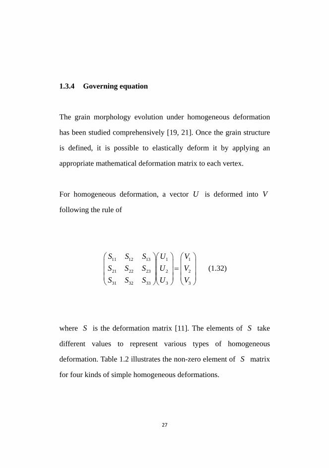
For homogeneous deformation, a vector U is deformed into V

following the rule of

11 12 13 1 1

21 22 23 2 2

31 32 33 3 3

S S S U VS S S U VS S S U V

⎛ ⎞⎛ ⎞ ⎛ ⎞⎜ ⎟⎜ ⎟ ⎜ ⎟=⎜ ⎟⎜ ⎟ ⎜ ⎟⎜ ⎟⎜ ⎟ ⎜ ⎟⎝ ⎠⎝ ⎠ ⎝ ⎠

(1.32)

where S is the deformation matrix [11]. The elements of S take

different values to represent various types of homogeneous

deformation. Table 1.2 illustrates the non-zero element of S matrix

for four kinds of simple homogeneous deformations.

28  

Table 1.2: Volume preserving deformation. The convention used is

that 11 22 33S S S> >

The grain shape evolution in homogeneous deformation can be

calculated by application of equation (1.32) to every pixel of the

grain body. For polyhedron grains, the morphological progressing is

computable by just considering the conversion of grain vertexes

during deformation [19]. Figure 1.10 demonstrated the changes of

shape of two neighbored grains before and after simple deformation

by vertexes transformation.

Type 11S 1S

13S 2S

22S 23S

31S

32S

33S

Plane strain compression

1≥ 0 0 0 1 0 0 0 11

1S

Axisymmetric compression 33

1S

0 0 033

1S

0 0 0 1≤

Axisymmetric tension

1≥ 0 0 011

1S

0 0 0 11

1S

Simple shear 1 0 +ve 0 1 0 0 0 1

29  

(a)

(b)

(c)

(d)

(e) Figure 1.10: Grain shapes at (a) No-deformed grains; (b) Plain

strain deformation; (c) Axisymmetric tension; (d) Axisymmetric

compression; (e) Simple shear.

30  

Furthermore, in terms of geometric concerns, equation (1.32) can be

applied to transform the lattices using finite difference method to

cope with the phase-field governing equation, which would change

the grain interface orientation. This enables the integration of phase

transition simulation with deformation simulation.

1.4 Aim of the work

The phase transformation during homogeneous deformation in steel

is the fundamental important phenomenon for understanding warm

rolling because the morphology of grain in steel plays important role

on mechanical properties of the steel.

The microstructure changes during deformation process, with an

increase in the grain geometry and grain distortion. The grain

distortion induced by the elastic deformation also causes the change

of grain interface orientation, which is relative to the ( )nε value in

phase-field model. This will result in completely different grain

morphology and change the microstructure development during

deformation while phase transition process in comparison of

deformation after phase transition process.

31  

In the previous studies, the formation and morphology of grain

growth for phase transition from austenite has been simulated.

However, to the author’s knowledge, no phase-field model, which

can treat the phase transformation under deformation, has been

proposed. In order to predict the microstructure evolution during

warm rolling, including the consequences on elementary mechanical

properties, a new phase-field model, which is able to describe the

phase transformation accompanying with the elastic deformation

should be developed. Due to the complex inter-connection between

deformation parameters and grain growth, more studies are still

required in order to understand material behavior during warm

rolling processes.

The main purpose of this study is to enable us to perform an

integrated numerical simulation for the microstructure design of

phase transition while rolling by coupling the phase-field model with

homogeneous deformation method. Grain growth in phase transition

is computed by phase-field model while the grain shape deformation

is calculated by transforming grid coordinates according to

homogeneous deformation matrix.

In the following section, we will reformulate the governing equation

of the phase-field model to simulate the grain growth with

32  

homogeneous deformation, including effects of grain geometry, and

corresponding anisotropy parameters. We then provide detailed

derivation of numerical methods. Finally, computed results for

microstructure evolution of grain growth at different times and the

effect of homogeneous deformation on the grain morphology are

conducted concerning accuracy of the numerical method.

33  

Chapter 2 Numerical methodology

2.1 Overview

In the past, the phase-field simulations showed that it is a general

and powerful technique for simulating the evolution of relatively

complex morphologies. Simulation could give important insights

into the role of specific material or process parameters on the

microstructure evolution in solidification and the shape and spatial

distribution of precipitates in phase transformation process.

In the phase-field model, the temporal evolution of the phase-field

variables, which represent the morphological evolution of the grains

or domains in the system, is given by a set of coupled partial

differential equations, one equation for each variable. In phase-field

simulation, the results were rather qualitative and for real alloys the

complicate quantitative simulation is difficult. The governing

34  

equations in the model contain many phenomenological parameters

and they are difficult to determine for real alloys. Moreover, massive

computer resources are required to resolve the evolution of the

phase-field variable at the interfaces appropriately and, at the same

time, cover a system with realistic dimensions.

In this section, we give the steps in phase-field model and provide

some of the numerical results with particular consideration when

solving partial derivate equations of the second order factor for

phase-field parameter ( , )x tφ by the generalized finite difference

method.

2.2 Numerical procedure 2.2.1 Lattices properties

Firstly, we initialize the lattices properties. We define suitable lattices

to represent the space that occupied by material. At the initial

condition, the lattice distance xΔ is uniform and it must be fine

enough to make sure there are a few grid points within the interfacial

region to resolve the interfacial profile of the phase-field variables.

Therefore, in this simulation the lattice distance is chosen as the one

quarter of the interface thickness so that four lattices can cover the

35  

interface. [22-23]

For the lattice depicted in Figure 2.1, the set of algebraic equation in

the simulation contains 1 2 3N N N× × equations and the same

number of unknowns for each phase-field variable.

Figure 2.1 Lattices depiction at initial condition. 2.2.2 Nucleation

The formation of a crystal involves nucleation. Basically, if the

nucleation occurs on a surface, such as a boundary of the system, or

on other body, such as a dust particle, it is heterogeneous nucleation.

If the structure and interatomic spacing of the surface on which

nucleation takes place approximate those of the crystal, growth on

1N

2N

3N

36  

the surface can resemble growth on a normal seed. This is called

epitaxial growth. If the nucleation occurs in the absence of a surface,

that is, in the bulk of unit cell, it is homogeneous.

The model of this work focus on growth of single crystal, which

occurs in the centre of the unit cell. Therefore, the second step is to

put the nuclei manually to the lattice space according to the classical

nucleation theory. The initial condition is to put a spherical seed with

a radius of r at the centre of the logistic frame with phase-field

order parameter configures to [16]

( , 0) 12( , 0) 4

1 exp( 1)( , 0) 0 4

r t for r x

r t for x r xr

r t for r x

φ

φ

φ

⎧ = = ≤ Δ⎪⎪ = = Δ < < Δ⎨ + −⎪⎪ = = ≥ Δ⎩

(2.1)

Then all the lattices should be specified with the initial value of its

phase-field order parameterφ , solute composition c and temperature

T . In the processing, the lattice with 0.1 0.9φ< < is interface,

0.1φ < is α and 0.9φ > is β phase.

2.2.3 Time step

The third step is to define the proper time step, which affects the

37  

stability of the finite-difference scheme which used for discreting the

governing equation of phase-field model. At each time step, the

value of the phase-field variables must be computed for all the grid

points. In this simulation, for the stability of computation, we can

directly use the necessary2

2xt Δ

Δ ≤ , where xΔ is the length of the

lattice. Moreover, smaller lattice spacing involves a smaller time step

in order to maintain numerical stability. Because of this, large

computer memory is also required to treat the huge algebraic

systems of equations with many unknown.

2.2.4 Non-dimensionalization

The fourth step is to non-dimensionalize the governing equations for

phase-field model. For the sake of computational stability, it is

normal to use dimensional variables in the governing equations so

that the occurrence of very small or very large numbers is avoided.

The parameters that used in equation (1.11) are non-dimensionalized

by using [24]:

/x x LΔ = , 20.3 / ct x DΔ = Δ , 2 /c c mM L RT D Vφ = ,

0 0 / /m cV RT Lε ε= , /c mRT Vω ω= and

38  

0 1 1 0( ) / ( )m cg g g g V RT− = − . 10nmL = is defined the

characteristic length. 6 310 m /molcD −= is the carbon diffusivity in

steel [27]. -1 -18.31J K molR = ⋅ is the gas constant.

6 37.18 10 m /molmV −= × is the molar volume of the material.

o369.8 CcT = is actually the martensitic transition temperature of

Fe_0.4wt%C steel.

After non-dimensionalizing the variables, they range roughly

between 0 and 1 and they are unnormailsed when interpreting the

outputs of the model.

Furthermore, to make sure that all the parameters are chosen with

practical ground rather than from pure fiction, the martenstic

transition of Fe_0.4wt%C steel at o250 C is referenced, MTDATA

thermodynamics database gives 9 20 1.73 10 J/mg = − × and

9 21 2.09 10 J/mg = − × . 2

0 800erg/cmk = is the experimental value

of interface energy in steel [26].

2.2.5 Discretization

The fifth step which is one of the most important steps is to discrete

39  

the governing equation of phase-field model. In the present work

finite difference formula is given for partial derivative equations of

the first and second order factors. In the past, the classic finite

difference method has been widely used due to the rapid

development of computer technology and big possibilities that this

offers when solving large series of equations. This classic method,

however, continued to be restricted by the enforced use of regular

meshes. A finite difference discretization technique using uniform

lattice spacing, and with a central second-order stepping in space and

forward stepping in time, is most widely used because of its

simplicity. However, as shown in Figure 2.2, after deformation, the

rectangular lattices will become non-rectangular, which is not

available for the classic finite difference method. Thus, we will use

another finite difference method which will be discussed later.

40  

Figure 2.2: (a) Square lattices before deformation. (b) Irregular

lattices during deformation. (c) Planes distortion during deformation

in three-dimension.

X 

Y

Z

.a .b

α

α

.c

41  

2.3 Finite-Difference Method

2.3.1 Overview

A significant number of physical and engineering problems lead to

differential equations with partial derivatives. Implicit solutions to

equations of mathematical physics are obtainable only in special

cases. Therefore these problems are generally solved approximately

by using some numerical method. In previous work, some

mathematically models integrated with the finite-element method to

predict the material behaviour during deformation [28-29].

Meanwhile, another method which is one of the most universal and

an effective method in wide use today for approximately solving

equations is the method of finite differences.

In classical numerical techniques there are some obstacles. It may be

difficult to find a simple function over the entire domain and if such

functions are found they could lead to large and complicated systems

of equations. However, through finite difference method, the

continuous domain is replaced by a discrete set of nodes and instead

of a function of continuous argument, a function of discrete

arguments is considered. The value of this function is defined at the

nodes of the grid or at other elements of the grid. The derivatives

42  

entering into the differential equations and the boundary conditions

are approximated by the difference expression, thus the differential

problem is transformed into a system of linear or non-linear

algebraic equations. Such system is often called the finite-difference

scheme.

In the simulation process, the finite difference method for differential

equation is carried out in the following stages. First is the writing of

the finite-difference scheme which means the difference

approximation to the differential equation on a grid. Second is the

computer solution for difference equations, which is written in the

form of a high-order system of linear or non-linear algebraic

equations.

2.3.2 General finite-difference method

In finite difference method, there are two main types of scalar

function of a discrete argument. In the first case, the values of the

function correspond to the nodes. This is nodal discretisation. In this

case, grid function hu is a set of M N× numbers:

{ }, 1, , ; 1, ,h hiju u i M j N= = = . The second possibility is

cell-valued discretisation. To denote the values of a cell-valued

43  

function, we will use the same procedure as for the mesh of a grid;

that is hiju as it is related to cell ijΩ . For the cell-centred

discretisation, index i varies in limits from 1 to 1M −

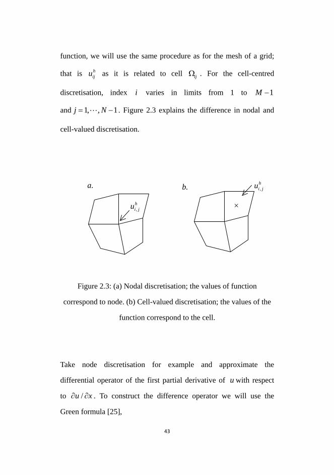
and 1, , 1j N= − . Figure 2.3 explains the difference in nodal and

cell-valued discretisation.

Figure 2.3: (a) Nodal discretisation; the values of function

correspond to node. (b) Cell-valued discretisation; the values of the

function correspond to the cell.

Take node discretisation for example and approximate the

differential operator of the first partial derivative of u with respect

to /u x∂ ∂ . To construct the difference operator we will use the

Green formula [25],

×

,hi ju  .b.a

,hi ju  

44  

0lim l

s

udyux S→

∂=

∂

∫ (2.2)

where S is the area bounded by contour l . In the discrete case, the

role S is played by the grid cell ijΩ . Therefore l is the union of

sides 1, , 1 ,, , ,ij i j i j i jl l l lξ η ξ η+ + as showed in Figure 2.4. For

approximation of the contour integral in the right-hand side of

equation (2.2), we divide the contour integral into four integral each

over the corresponding side of quadrangle ijΩ and for the

approximate evaluation of each integral, we use the trapezium rule.

As a result, we obtain the following expression for the difference

analog of derivative /u x∂ ∂ :

1, 1 , , 1 1, , 1 1, 1, 1 ,( )( ) ( )( )( )

2i j i j i j i j i j i j i j i jh

x ijij

u u y y u u y yD u + + + + + + + +− − − − −

=Ω

(2.3)

45  

Figure 2.4: Stencil for operator xD

In the example of xD we can demonstrate the notion stencil of

difference operators in 2-D. The stencil is a set of nodes that

participate in the formula for discrete operators. Therefore, the

stencil of operator xD in cell ( , )i j contains

nodes ( , ), ( 1, ), ( 1, 1), ( , 1)i j i j i j i j+ + + + .

2.3.3 Application of finite-difference method

The finite difference method is a technique used principally for

,( )hx i jD u

ijΩ

, 1i jlξ +  

1,i jlη +  

,i jlη  

,i jlξ  

×

, 1hi ju +

1, 1hi ju + +  

1,hi ju +  

,hi ju  

46  

solving partial differential equation approximately. The method is

not synonymous with any physical theory, although its heaviest use

probably has been in solid and structural mechanics. While there are

a few features common to all finite difference formulation, there is

no single universal formulation. Rather, there is considerable variety

in the implementations of the method, usually motivated by aspects

of the system of equations being solved.

In the simulation, the direction of each plane in the classical

phase-field model will be changed because of the homogeneous

deformation. Figure 2.2 schematically shows how meshes are

changed during deformation process. Figure 2.5 shows directions of

each plane from one random point in three dimension and Figure 2.6,

Figure 2.7 and Figure 2.8 show the lattices evolution in the three

directions during deformation.

47  

Figure 2.5: Direction of each plane from one random point in the

lattices.

α

β

γxz

y

xz

y

γ

α

xz

yβ

x

z

y

48  

Figure 2.5: The irregular lattices in α plane during deformation.

Nevertheless, considering α plane in three dimensions, based on

irregular lattices as showed in Figure 2.5 and finite difference

method, we can get the formula

In α plane:

, ,, 1, , 1, 1, , 1, , 1, , 1, , , 1, , 1,

1 ( )( ) ( )( )2

i j ki j k i j k i j k i j k i j k i j k i j k i j k

α

φφ φ β β φ φ β β

α + − − + − + + −

∂⎡ ⎤= − − − − −⎣ ⎦∂ Ω

(2.4)

(i+1,j‐1,k) 

x  

y

z

αβ

n

α

(i,j,k)

(i,j+1,k) 

(i,j‐1,k) 

(i+1,j,k) 

(i+1,j,k)

(i+1,j+1,k) 

(i‐1,j‐1,k) 

(i‐1,j+1,k) 

49  

2, , ( 1, 1, ) ( 1, 1, )

( 1, 1, ) ( 1, 1, )2

1 [( )( )2

i j k i j k i j ki j k i j k

α

φ φ φβ β

α α α+ + − −

− + + −

∂ ∂ ∂= − −

′∂ Ω ∂ ∂

( 1, 1, ) ( 1, 1, )( 1, 1, ) ( 1, 1, )( )( )]i j k i j ki j k i j k

φ φβ β

α α− + + −

+ + − −

∂ ∂− − −

∂ ∂

(2.5)

2, , ( 1, 1, ) ( 1, 1, )

( 1, 1, ) ( 1, 1, )1 [( )( )

2i j k i j k i j k

i j k i j kα

φ φ φβ β

α β β β+ + − −

− + + −

∂ ∂ ∂= − −

′∂ ∂ Ω ∂ ∂

( 1, 1, ) ( 1, 1, )( 1, 1, ) ( 1, 1, )( )( )]i j k i j ki j k i j k

φ φβ β

β β− + + −

+ + − −

∂ ∂− − −

∂ ∂

(2.6)

where αΩ is the area of quadrangle which connect points

( , 1, ), ( , 1, ), ( 1, , )i j k i j k i j k+ − + and ( 1, , )i j k− . α′Ω is the area

of quadrangle which connect points

( 1, 1, ), ( 1, 1, ), ( 1, 1, )i j k i j k i j k+ + − + + − and ( 1, 1, )i j k− − in

Figure 2.5.

50  

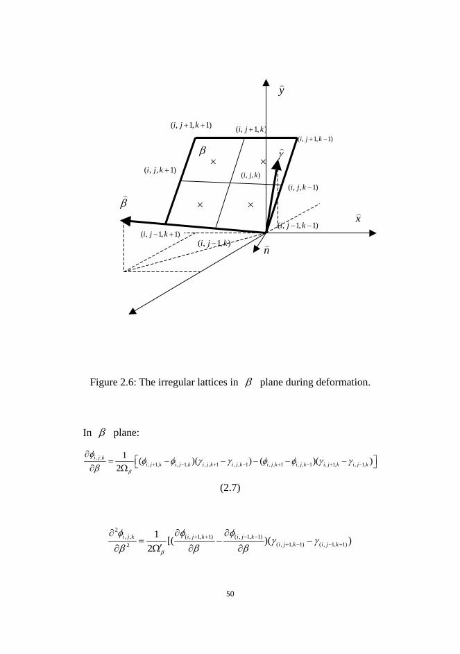
Figure 2.6: The irregular lattices in β plane during deformation.

In β plane:

, ,, 1, , 1, , , 1 , , 1 , , 1 , , 1 , 1, , 1,

1 ( )( ) ( )( )2

i j ki j k i j k i j k i j k i j k i j k i j k i j k

β

φφ φ γ γ φ φ γ γ

β + − + − + − + −

∂⎡ ⎤= − − − − −⎣ ⎦∂ Ω

(2.7)

2, , ( , 1, 1) ( , 1, 1)

( , 1, 1) ( , 1, 1)2

1 [( )( )2

i j k i j k i j ki j k i j k

β

φ φ φγ γ

β β β+ + − −

+ − − +

∂ ∂ ∂= − −

′∂ Ω ∂ ∂

× ×

× ×x

y

β

γ

n

( , 1, 1)i j k+ +

( , , 1)i j k +

( , 1, 1)i j k− +( , 1, )i j k−

( , 1, 1)i j k− −

( , , 1)i j k −

( , 1, 1)i j k+ −( , 1, )i j k+

( , , )i j k

β

51  

( , 1, 1) ( , 1, 1)( , 1, 1) ( , 1, 1)( )( )]i j k i j ki j k i j k

φ φα α

β β+ − − +

+ + − −

∂ ∂+ − −

∂ ∂

(2.8)

2, , ( , 1, 1) ( , 1, 1)

( , 1, 1) ( , 1, 1)1 [( )( )

2i j k i j k i j k

i j k i j kβ

φ φ φβ β

β γ β β+ + − −

+ − − +

∂ ∂ ∂= − −

′∂ ∂ Ω ∂ ∂

( , 1, 1) ( , 1, 1)( , 1, 1) ( , 1, 1)( )( )]i j k i j ki j k i j k

φ φβ β

β β+ − − +

+ + − −

∂ ∂− − −

∂ ∂

(2.9)

where βΩ is the area of quadrangle which connect points

( , 1, ), ( , 1, ), ( , , 1)i j k i j k i j k+ − + and ( , , 1)i j k − . β′Ω is the area

of quadrangle which connect points

( , 1, 1), ( , 1, 1), ( , 1, 1)i j k i j k i j k+ + − − + − and ( , 1, 1)i j k− + in

Figure 2.6

Figure 2.7: The irregular lattices in γ plane during deformation.

52  

In γ plane:

, ,, , 1 , , 1 1, , 1, , 1, , 1, , , , 1 , , 1

1 ( )( ) ( )( )2

i j ki j k i j k i j k i j k i j k i j k i j k i j k

γ

φφ φ α α φ φ α α

γ + − − + − + + −

∂⎡ ⎤= − − + − −⎣ ⎦∂ Ω

(2.10)

2, , ( 1, , 1) ( 1, , 1)

( 1, , 1) ( 1, , 1)2

1 [( )( )2

i j k i j k i j ki j k i j k

γ

φ φ φα α

γ γ γ+ + − −

− + + −

∂ ∂ ∂= − −

′∂ Ω ∂ ∂

( 1, , 1) ( 1, , 1)( 1, , 1) ( 1, , 1)( )( )]i j k i j ki j k i j k

φ φα α

γ γ− + + −

+ + − −

∂ ∂+ − −

∂ ∂

(2.11)

2, , ( 1, , 1) ( 1, , 1)

( 1, , 1) ( 1, , 1)1 [( )( )

2i j k i j k i j k

i j k i j kγ

φ φ φγ γ

α γ γ γ+ + − −

− + + −

∂ ∂ ∂= − −

′∂ ∂ Ω ∂ ∂

( 1, , 1) ( 1, , 1)( 1, , 1) ( 1, , 1)( )( )]i j k i j ki j k i j k

φ φγ γ

γ γ− + + −

+ + − −

∂ ∂− − −

∂ ∂

(2.12)

where γΩ is the area of quadrangle which connect points

( , , 1), ( , , 1), ( 1, , )i j k i j k i j k+ − − and ( 1, , )i j k+ . γ′Ω is the area

of quadrangle which connect points

( 1, , 1), ( 1, , 1), ( 1, , 1)i j k i j k i j k+ + + − − − and ( 1, , 1)i j k− + in

53  

Figure 2.6

These formulas are for cell-centred discretisation and they refer to a

group of established nodes related to one, which is denoted as central

node. For calculating the value of one point, we have to use 21

neighbouring points. Actually, there is no best method way for

obtaining approximating difference formulae, and as many different

methods as possible will be tested. The only requirement is that the

formula, having been obtained, must pass certain test of accuracy,

consistency, stability and convergence.

During deformation, each quadrangle will probably have different

shape. For the purpose of the program we define a set of parameters

for viewing arbitrary planes through deformation, which is easy to

visualize for the user. Therefore, we have to use coordinate

transformation to make all the phase-field governing equation of

each point can be explained in one coordinate.

2.4 Coordinate transformation

2.4.1 General coordinate transformation

54  

The need for the use of more than one coordinate system comes from

the fact that many different physical phenomena are easier calculated

or understood in a system that is appropriate for the phenomenon.

Frequently, it is quite necessary to transform from one coordinate

system to another.

For the definition of a coordinate system in three-dimensional space,

one has only to specify the direction of one of the axes, and the

orientation of one of the other axes in the plane perpendicular to this

direction. The third axis follows automatically in order to complete a

right-handed orthogonal set. As showed in Figure 2.5, α means the

direction along the irregular lattices. β is perpendicular to α and

n is the normal direction of α plane which means a random plane

in the model. The coordinate systems and transformations used in

this simulation are Cartesian coordinates system.

In Cartesian coordinate system, a position vector M in a

three-dimensional space can be represented in vector form as

m m m m m m m mr O M x i y j z k= = + + (2.13)

where ( , , )m m mi j k are the unit vectors of coordinate axes, and by the

55  

column matrix it can written as:

m

m m

m

xr y

z

⎡ ⎤⎢ ⎥= ⎢ ⎥⎢ ⎥⎣ ⎦

(2.14)

The subscript m indicates that the position vector is represented in

coordinate system ( , , )m m m mS x y z . There are many ways to define an

arbitrary rotation, scaling and translation of one coordinate frame

into another. Consider two coordinate systems ( , , )m m m mS x y z and

( , , )n n n nS x y z as an example. Point M is represented in coordinate

system mS by the position vector as:

[ ]1 Tm m m mr x y z= (2.15)

In coordinate system nS the same point can be determined by the

position vector as:

[ ]1 Tn n n nr x y z= (2.16)

56  

with the matrix equation:

n nm mr M r= (2.17)

Matrix nmM is represented by:

11 12 13 14

21 22 23 24

31 32 33 34

0 0 0 1

nm

a a a aa a a a

Ma a a a

⎡ ⎤⎢ ⎥⎢ ⎥=⎢ ⎥⎢ ⎥⎣ ⎦

( ) ( ) ( ) ( )

( ) ( ) ( ) ( )

( ) ( ) ( ) ( )0 0 0 1

n m n m n m n m n

n m n m n m n m n

n m n m n m n m n

i i i j i k O O i

j i j j j k O O j

k i k j k k O O k

⎡ ⎤⋅ ⋅ ⋅ ⋅⎢ ⎥

⋅ ⋅ ⋅ ⋅⎢ ⎥= ⎢ ⎥⋅ ⋅ ⋅ ⋅⎢ ⎥⎢ ⎥⎣ ⎦

( )

( )

( )

cos( , ) cos( , ) cos( , )

cos( , ) cos( , ) cos( , )

cos( , ) cos( , ) cos( , )0 0 0 1

m

m

m

On m n m n m n

On m n m n m n

On m n m n m n

x x x y x z x

y x y y y z y

z x z y z z z

⎡ ⎤⎢ ⎥⎢ ⎥

= ⎢ ⎥⎢ ⎥⎢ ⎥⎣ ⎦

(2.18)

Here, ( , , )n n ni j k are the unit vectors of the axes of the new

coordinate system; ( , , )m m mi j k are the unit vectors of the axes of

the original coordinate system; nO and mO are the origins of the

57  

new and original coordinate systems; subscript nm in the

designation nmM indicates that the coordinate transformation is

performed from mS to nS . The determination of elements

( 1, 2,3,4; 1,2,3)lka k l= = of matrix nmM is based on the

following rules. Firstly elements of the 3 3× submatrix

11 12 13

21 22 23

31 32 33

nm

a a aL a a a

a a a

⎡ ⎤⎢ ⎥= ⎢ ⎥⎢ ⎥⎣ ⎦

(2.19)

represents the direction cosines of the original unit vectors

( , , )m m mi j k in the new coordinate system nS . The number l

indicates the original coordinate axis and the number k indicates the

new coordinate axis. Axes , ,x y z are given number 1, 2 and 3,

respectively. Elements 14 14,a a and 34a represent the new

coordinates ( ) ( ) ( ), ,m m mO O On n nx y z of the original mO .

2.4.2 Application of coordinate transformation

Using the coordinate transformation rule discussed above and taking

58  

α plane as an example, we can get:

1, , , , 1, , , , 1, , , ,2

1, , , ,

( ) ( ) ( )i j k i j k i j k i j k i j k i j k

i j k i j k

x x x y x y z z zα

α α+ + +

+

− + − + −=

− (2.20)

2

1, , , ,i j k i j k

nαββ β+

×=

− (2.21)

According the equations (2.17) and (2.18), the relationships between

these transformations are found by directly comparison of the

transformation matrix elements:

x y z

x y z

x n y n z n

i i i j i k xj i j j j k y

n k i k j k k z

α α α

β β β

αβ

⎛ ⎞∂ ⋅ ⋅ ⋅ ∂⎛ ⎞ ⎛ ⎞⎜ ⎟⎜ ⎟ ⎜ ⎟∂ = ⋅ ⋅ ⋅ ∂⎜ ⎟⎜ ⎟ ⎜ ⎟

⎜ ⎟ ⎜ ⎟⎜ ⎟∂ ⋅ ⋅ ⋅ ∂⎝ ⎠ ⎝ ⎠⎝ ⎠

(2.22)

where ,x yi i and zi are the unit vectors of the XYZ system, and

,i iα β and ni are the unit vectors of the nαβ system.

Furthermore, in XYZ system, the first order partial derivatives

were discretized by using

59  

nx x x x

ny y y y

nnz z z z

φ α β φα

φ α β φβφφ α β

⎛ ⎞ ⎛ ⎞⎛ ⎞∂ ∂ ∂ ∂ ∂⎜ ⎟ ⎜ ⎟⎜ ⎟∂ ∂ ∂ ∂ ∂⎜ ⎟ ⎜ ⎟⎜ ⎟∂ ∂ ∂ ∂ ∂⎜ ⎟ ⎜ ⎟⎜ ⎟=⎜ ⎟ ⎜ ⎟⎜ ⎟∂ ∂ ∂ ∂ ∂

⎜ ⎟ ⎜ ⎟⎜ ⎟∂∂ ∂ ∂ ∂⎜ ⎟ ⎜ ⎟⎜ ⎟

⎜ ⎟⎜ ⎟ ⎜ ⎟ ∂∂ ∂ ∂ ∂ ⎝ ⎠⎝ ⎠ ⎝ ⎠

(2.23)

0nφ∂=

∂ (2.24)

According to the nodes in the cell we want to get discretation value

and the lattices geometry, using equations discussed above, we can

derive the formula for operator , ,i j k

xφ∂∂

, , ,i j k

yφ∂∂

, , ,i j k

zφ∂∂

, 2

, ,2

i j k

xφ∂∂

,

2, ,2

i j k

yφ∂∂

, 2

, ,2

i j k

zφ∂∂

, 2

, ,i j k

xyφ∂∂

, 2

, ,i j k

yzφ∂∂

and 2

, ,i j k

xzφ∂∂

in the similar

way by using the 21-neighbor points and geometry of the cell in

three dimensions.

2.5 Conclusion

All spatial derivatives in phase-field governing equation were

discretized using finite difference formulas that we generalized

above. ( , , )i j k denotes the position of the node along the ,x y

and z axes, respectively. The second order partial derivatives were

60  

discretized using the nine-point formula. Time stepping was done

using a first-order Euler scheme.

From the above discussion, it may be seen that using finite difference

method and coordinate transformation method on phase-field model

depends on the following factors:

a. The position of nodes. This underlines the great importance of

the selection of nodes of the lattices. The selection or placement

of the nodes has a great influence on the results. Normally, when

selecting the nodes surrounding the central node, we selected

those closest to the central one in the Cartesian coordinates.

b. The relative coordinate of the lattice spacing. This is more

important in heterogeneous deformation because the neighbour

lattice maybe undergo deformation in different directions.

61  

Chapter 3 Simulation and discussion

3.1 Overview

Ideally, in an attempt to reduce experimental costs improve the

understanding of the mechanism, one would like to make a

prediction of a new material’s behaviour by numerical simulation,

with the primary goal being to accelerate trial and error experimental

testing. Simulation raises the possibility that modern numerical

methods can play a significant role in analysis of microstructure

evolution.

3.2 Simulation

62  

3.2.1 System diagram

According to the numerical procedures, which were discussed in

chapter 2, we can get the results of the simulation. As described in

chapter 1, there are four main types of homogeneous deformations.

And in this numerical simulation, we combined phase-field model

with simple shear deformation together. According to Table 1.2

which shows different value of S matrix, during simple shear

deformation, 11 22 33 1S S S= = = , 13S is the shear value, and all the

other elements of S are zero. Furthermore, for simplicity and to

ensure mechanical equilibrium, we assume uniform density and

temperature throughout the system and that there is no mass and

temperature diffusion in the phase.

As discussed in chapter 2, Figure 3.1 is the system diagram.

63  

Figure 3.1: System diagram of whole simulation

Bulk 

thermodynamics 

 

Interfacial energies 

Structural parameters 

Response functions 

Atomic  and

interface 

mobility 

New model 

‐Phase‐field parameter  φ  

‐Deformation type 

‐Deformation matrix  S

Spatial  and

temporal 

microstructures

Responses  of

microstructure 

Microstructure 

information 

databases

Information databases 

‐Initial grain shape 

‐Initial lattice properties 

‐Dimension 

‐Nucleus 

‐Boundary conditions 

64  

3.2.2 Parameters of simulation

The simulations were performed on a cubic grid of size

1 2 3 160 160 120N N N× × = × × with initial constant grid spacing.

Simulations were started with a small spherical seed in the corner of

the cubic. After deformation, lattices geometry such as grid spacing

is not constant anymore.

The phase-field governing equation contains many

phenomenological parameters, which are difficult to determine for

real alloys. In this simulation, the thermodynamic data for the

martenstic transition of Fe_0.4wt%C steel at o250 C is used. In

metallic materials the thickness of interface is about 3 to 5 atomic

distances which is about 1 nm but in this model the half thickness of

the interface is chosen as 14.3nm to accelerate the simulation

without losing much details of the grain morphology. The lattice

distance was chosen as 7.15nmxΔ = so that there are four grids

across the interfaces. According to the MTDATA thermodynamic

database, bulk free energy 9 20 1.73 10 J/mg = − × and

9 21 2.09 10 J/mg = − × . The interface energy is 2800erg/cm [26].

Three sets of anisotropy coefficients are applied in the simulation, as

list in Table 3.1. Figure 3.1 demonstrates the three different grain

65  

morphology without deformation using different interface anisotropy

in Table 3.1.

Case A Case B Case C

1k −0.863 0.402 0.0

2k 0.395 0.00144 0.0

3k 0.0238 0.00066 0.0

Table 3.1: Different sets of anisotropic coefficients

66  

Figure 3.1 Grain morphology at 5000 time steps under different

interface anisotropy list in Table 3.1. (a) Case A, (b) Case B and (c)

Case C.

.a

.b .c

67  

3.2.3 Results

Figure 3.2, 3.4 and 3.6 show the microstructure evolution in three

different sets of anisotropy parameters. Three types of different grain

growth under each anisotropic parameter are simulated. One is

normal grain growth without deformation. The second is simple

shear deformation along the y -axis after grain growth. The third is

the grain growth while undergoing homogeneous deformation along

the y -axis.

Figure 3.3, 3.5 and 3.7 show microstructure evolution in different

time steps while undergoing simple shear deformation using three

different anisotropy parameters.

68  

Case A (Dendrite)

Without deformation; time steps=12000

Deformation after grain growth; time steps=12000

Deformation during grain growth; time steps=12000

Figure 3.2: Grain morphology at 100Mφ = computation using

anisotropy coefficient in Case A: (a) No simple shear deformation; (b)

With simple shear deformation after grain growth for 12000 time

.a

.b

.c

69  

steps; (c) After 12000 time steps with simple shear deformation in

every 6000 time steps while grain growth.

Case A (Dendrite)

Time steps=6000 Time steps=8000

Time steps=10000 Time steps=12000

z  x

y

70  

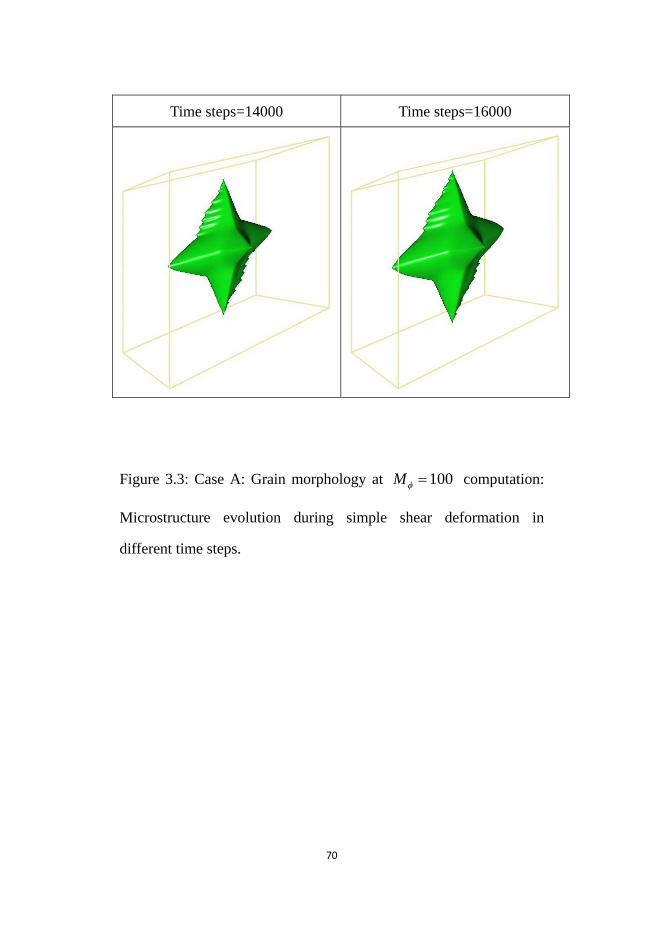
Time steps=14000 Time steps=16000

Figure 3.3: Case A: Grain morphology at 100Mφ = computation:

Microstructure evolution during simple shear deformation in

different time steps.

71  

Case B (Cubic)

Without deformation

Deformation after grain

growth;

time steps=18000

Deformation during grain

growth;

time steps=18000

Figure 3.4: Grain morphology at 100Mφ = computation using

72  

anisotropy coefficient in Case B: (a) No simple shear deformation; (b)

With simple shear deformation after grain growth for 18000 time

steps; (c) After 18000 time steps with simple shear deformation in

every 6000 time steps while grain growth.

Case B (Cubic)

Time steps=4000 Time steps=6000

73  

Time steps=10000 Time steps=12000

Time steps=16000 Time steps=18000

Figure 3.5: Case B: Grain morphology at 100Mφ = computation:

Microstructure evolution during simple shear deformation in

different time steps.

74  

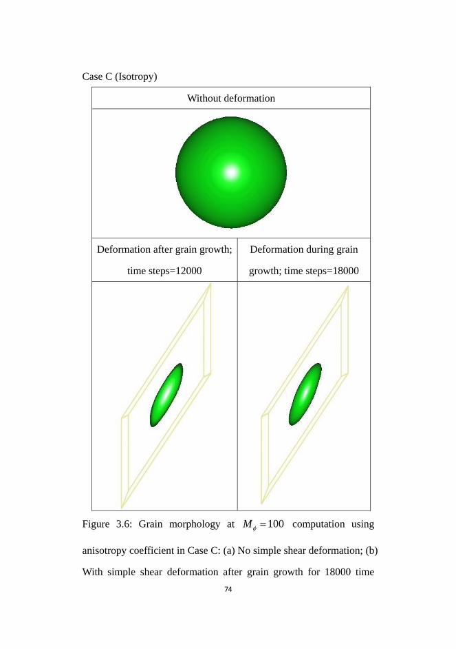
Case C (Isotropy)

Without deformation

Deformation after grain growth;

time steps=12000

Deformation during grain

growth; time steps=18000

Figure 3.6: Grain morphology at 100Mφ = computation using

anisotropy coefficient in Case C: (a) No simple shear deformation; (b)

With simple shear deformation after grain growth for 18000 time

75  

steps; (c) After 18000 time steps with simple shear deformation in

every 6000 time steps while grain growth.

Case C (Isotropy)

Time steps=4000 Time steps=6000

Time steps=10000 Time steps=12000

76  

Time steps=16000 Time steps=18000

Figure 3.7: Case C: Grain morphology at 100Mφ = computation:

Microstructure evolution during simple shear deformation in

different time steps.

3.3 Discussion

As demonstrated earlier, three different processing bring out three

different microstructure evolutions and the morphology of the

growing grain presents here to minimize the free energy of the whole

system. In addition, after a particular time step, the new

77  

microstructure disappears step by step which because of the effect of

grain growth rate is more effective than the effect of the change in

normal interface vector.

In solid state, the interactions between atoms in crystal are stronger.

Thus the atoms are able to move only in vibrations of extremely low

amplitude about fixed positions relative to one another. As a result,

solids have rigidity, fixed shape, and mechanical strength.

Furthermore, when a force of any magnitude is applied to a solid

body the body becomes distorted; that is, some part of the body

moves with respect to some neighbouring portion. As a result of this

displacement the atomic attractive forces in the body set up restoring

forces that resist the alteration and tend to restore the body to its

original shape. The restoring force in a deformed body is termed

stress and has the units of force per area. The dimensional change

produced by an applied force is called strain.

One effect of simple shear deformation on microstructure evolution

is the direct grain distortion which will change the grain size and

grain size distribution in phase transformation. Subsequently, this

will change the grain interface orientation and normal vector n as

showed in Figure 3.8.

78  

Figure 3.8: schematic diagram of interface orientation evolution

during deformation.

The normal direction of grain interface n is related with the

anisotropy surface energy in equation (1.12). Furthermore, it will

change the grain interface migration pattern and eventually lead to

the change of grain morphology compared with deformation after

phase transformation.

To more specifically explain this phenomenon, we assuming an

operator G to represent the grain growth in Cartesian coordinates:

( ) ( ) ( ) ( )x y zG n G n G n G n⎡ ⎤= ⎣ ⎦ (3.1)

Grain growth in phase transition while undergoing deformation can

be described:

( )t

total ij it o

G S G n=

= ⋅∑ (3.2)

n n

79  

where iG means grain growth matrix after i th deformation.

Meanwhile, grain growth in phase transition before deformation:

[ ( ) ]t

total ijt o

G G n S=

′ = ∑ (3.3)

Because the normal unit vector of interface n is related to the

deformation operator ijS , so

total totalG G′≠ (3.4)

when the anisotropic effect of interface is ignored, total totalG G′= .

Therefore, from the equations discussed above, it is reasonable that

the microstructure obtain by phase transition during deformation can

been completely different from that deformation after phase

transiton.

Figure 3.9 describes the whole change of lattices in three different

situations. One is normal grain growth without deformation. Second

one is simple shear deformation along the y -axis after grain growth.

The last one is grain growth while undergoing homogeneous

deformation along the y -axis. Figure 3.10, 3.11 and 3.12 show the

cross-section of grain growth in phase transition during deformation

and after deformation along three axes.

80  

b

c

Figure 3.9: Distortion of the whole unit cell. (a) No deformation. (b)

Deformation during grain growth. (c) Deformation after grain

growth.

x

y

z

x

y

z   x

y

z

81  

a .

b .

c .

Figure 3.10: Cross-section in z-direction of grain: (a) no deformation;

(b) Simple shear deformation while grain growth; (c) simple shear

deformation after grain growth

x

y

82  

a .

b .

c .

Figure 3.11: Cross-section in y-direction of grain: (a) simple shear

deformation while grain growth; (b) simple shear deformation after

grain growth.

x

z

83  

Figure 3.12: Cross-section in x-direction of grain: (a) No

deformation; (b) Simple shear deformation while grain growth; (c)

Simple shear deformation after grain growth.

y

z

84  

In simple shear deformation, the shearing force is applied to a body

the amount of slide or shear between two layers unit distance apart is

shear strain. Hook’s law states that stress is proportional to strain

within the elastic limit, that is, within the range of forces where the

body will recover its original shape when the forces are removed.

Furthermore, if a material is strained in a particular direction the

crystallites will usually be elongated in the same direction. In Figure

3.9, the simple shear deformation is in y axis which changes the

position of each points in y direction. From the lattice sections of

each direction in Figure 3.10, 3.11 and 3.12, lattices distorted in xy

plane and elongated in xz plane.

In xy plane, meshed are distorted because of the simple shear

deformation along y axis. The normal vector of the interface is

changed which result the grain growth to different direction. From

Figure 3.13, after simple shear deformation, grain growth according

to the new vector n′ which result the new microstructure.

85  

a.

b.

Figure 3.13: Normal vector of interface. (a) No deformation. (b)

During deformation. n means normal vector of the interface before

deformation. n′ represents the new normal vector after

deformation.

In xz plane, there is no as big difference of microstructure as in

yz plane. The distances of the lattice elongate in x direction and

shorten in z direction. This results diffusion of phase-field

parameter φ in z direction a little bit faster than it in deformation

after grain growth. Therefore, the grain growth is faster in z

direction which also showed in Figure 3.12.

n

n′

86  

In yz plane, there is no lattice change which result the same

microstructure evolution.

In conclusion, the strain will usually tend to partially orient the

distorted crystallites. The glide planes and glide directions in

crystallites tend to become parallel to the deformation direction. In

material, such preferential orientation is called texture. Texture will

often persist through subsequent recrystallization. In this simulation,

after once deformation, the grain growth direction changes and

persists in new direction before second deformation.

In cubic and isotropic situation, there are no big differences in

microstructure evolution because their anisotropy of interface energy

is small.

Actually, in most of the solid materials, the individual crystals are

rather small and materials contain many of these crystallites. Each of

these crystallites is misoriented with respect to its neighbours to a

greater or lesser degree. Often these crystallites are called grains, and

the regions between crystallites are called grain boundary, where

nucleation has more chances to happen than inside the grains. Figure

3.14 illustrates how nucleation happens in the grain boundary [20].

From the simulation results, deformation happens during phase

transition makes different area of grain boundary and this changes

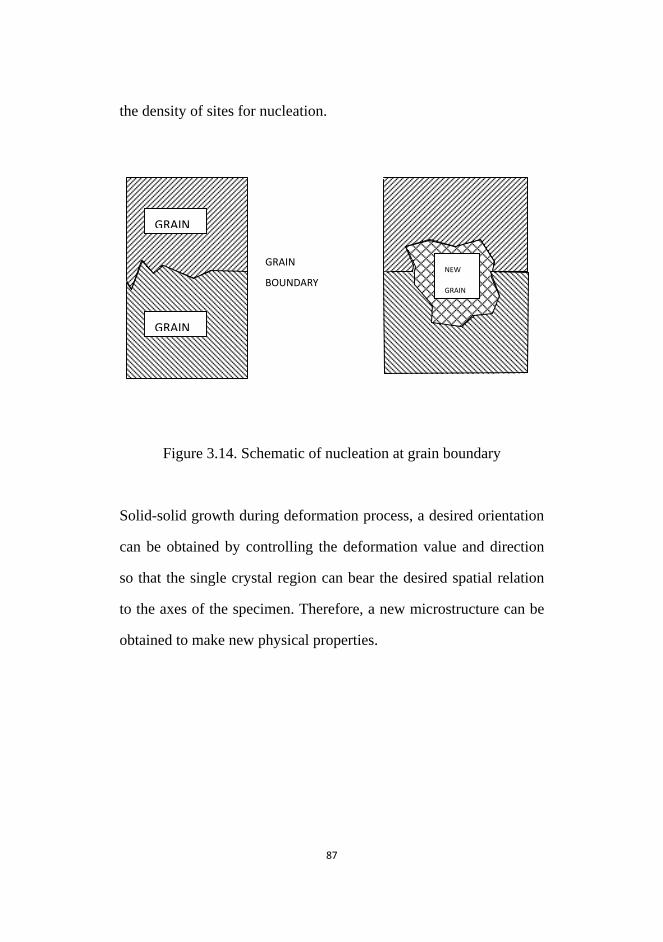
87  

the density of sites for nucleation.

Figure 3.14. Schematic of nucleation at grain boundary

Solid-solid growth during deformation process, a desired orientation

can be obtained by controlling the deformation value and direction

so that the single crystal region can bear the desired spatial relation

to the axes of the specimen. Therefore, a new microstructure can be

obtained to make new physical properties.

GRAIN

GRAIN

GRAIN 

BOUNDARY NEW 

GRAIN

88  

3.4 Conclusion

The physical properties of all technologically interesting materials

are strongly dependent upon their chemical composition as well as

their microstructure. The most efficient way of obtaining the

desirable microstructure is via accurate control of phase

transformation in solids. Phase transition requires two processes:

nucleation and growth. Nucleation involves the formation of very

small particles. During growth, the nuclei grow in size at the expense

of the surrounding material.

The structure resulting from a solid state phase transformation

depends on the crystallographic relationship between the lattices of

the initial and product phases, on the physical properties of the

separate phases, and on the rate of the transformation. There are

many phase transformations which are not limited by diffusion, but

result simply from some form of mechanical instability of the crystal

lattices, and may require some form of structural transition from one

crystallographic lattice to another. Thus, a homogeneous movement

of many atoms may results in a change in crystalline structure by

introducing an entirely new lattices and corresponding unit cell.

During the movements the atoms typically maintain their relative

relationships which are showed in the results.

89  

According the results of the simulation, a new microstructure is

obtained which can give us new physical properties. There is no

mass diffusion in this model. Thus, in the further work, basic on this

model we can add composition diffusion and simulation more crystal

in one system which related to the texture.

90  

Chapter 4 Conclusion

The effect of various deformations in phase transition is important

because it can change the way of grain growth. The aim of this work

was to simulate the effect of homogeneous deformation in phase

transition. First we described the problem of calculating the

microstructure evolution for homogeneous deformation and then

provided a detailed numerical method and methodology for solving

the three-dimension phase-field model to simulate such

microstructure evolution in phase transition while warm rolling.

From this work, we know homogeneous deformation in phase

transition will cause not only the change of lattice geometry used in

phase-field model but also cause the grain distortion which related

with the interface migration pattern. Subsequently, the

microstructure that obtained by phase transition during warm rolling

can be completely different from that rolling after phase transition.

91  

Metal with new microstructure and therefore new properties can be

obtained by this processing.

Meanwhile, in the process of simulation, phase-field model

combined finite difference method, viewed solely as a framework

motivated by the physics of deformation in the microstructure,

provides the finite difference analyst benefit as compared to the more

common model. The simulation captures the underlying physics of

metal deformation to a greater degree.

The whole work provides a method to simulate phase-field model in

irregular lattice using general finite difference method. And the

results of the simulation show that the microstructure evolution of

deformation while phase transition could be different compared with

deformation after phase transition.

92  

REFERENCES 1. Haldar and R.K. Ray. Microstructural and textural development I: an

extra low carbon steel during warm rolling, Mater. Sci. Eng. A 391 (2005), p. 402.

2. G.H. Akbari, C.M. Sellars and J.A. Whiteman. Acta Mater. 45 (1997), p. 5047–5058.

3. J Majta and A.K. Zurek. Modeling of ferrite structure after deformation in the two-phase region, Int. J. Plasticity 19 (2003), p. 707–730.

4. B.Koohbor, D.Ohadi, S.Serajzadeh and J.M.Akhgar. Effect of rolling speed on the occurrence of strain aging during and after warm rolling of a low-carbon steel. Journal of Material Science (2009), p. 3405-3412

5. D. Liu, A.O. Humphreys, M.R. Toroghinezhad and J.J. Jonas. The

Deformation Microstructure and Recrystallization Behavior of Warm Rolled Steels; ISIJ Intl., 42, (2002), p. 751-759.

6. S. Serajzadeh and M. Mohammadzadeh. Effects of deformation

parameters on the final microstructure and mechanical properties in warm rolling of a low-carbon steel, Int. J. Adv. Manuf. Tech. (2006), p. 262-269

7. N. Moelans, B. Blanpain, P.Wollants, Calphad, An introduction to phase-field modeling for microstructure evolution. Vol. 32: 268-294 (2008)

8. J. Fix, in Free Boundary Problems: Theory and Applications, Ed. A. Fasano and M. Primicerio, p. 580, Pitman (Boston, 1983)

93  

9. J.S. Langer, Models of pattern formation in first–order phase transitions, in Directions in Condensed Matter Physics p. 165, Ed. World Scientific, Singapore, (1986)

10. John W. Cahn and John E. Hilliard. Free energy of a nonuniform system. Nucleation in a two-component incompressible fluid. The Journal of Chemical Physics. (1959). p. 688-699

11. Cahn, J.W., On spinodal decomposition in cubic crystals, Acta Met.,

Vol. 10, p. 179 (1962)

12. A. A. Wheeler, W. J. Boettinger and G. B. McFadden. Phase-field model for isothermal phase transition in binary alloys. Physical Review A. Vol. 45, p. 7424-7439 (1992)

13. J. A. Warren and W. J. Boettinger. Prediction of dendritic growth and microsegegation patterns in a binary alloy using the phase-field method. Acta metal. Vol. 43, p. 689-703 (1994)

14. A.A. Wheeler, B.T. Murray and R.J. Schaefer. Computation of dendrites using a phase field model, Physica D (1993), p. 243–262.

15. J. W. Cahn and D. W. Hoffman, "A Vector Thermodynamics for Anisotropic Surfaces. II. Curved and Facetted Surfaces," Acta Met. 22, 1205-1214 (1974).

16. R.S. Qin and H.K.D.H. Bhadeshia. Phase-field model study of the effect of interface anisotropy on the crystal morphological evolution of cubic metals. Acta Mater 57 (2009), p. 2210.

17. A. A. Wheel, W. J. Boettinger and G. B. McFadden. Phase-field model for isothermal phase transition in binary alloys. Phys. Rev. A 45, 7424 (1992).

18. Seong Gyoon Kim, Won Tae Kim and Toshio Suzuki. Interfacial compositions of solid and liquid in a phase-field model with finite

94  

interface thickness for isothermal solidification in binary alloys. Phys. Rev. E. 58, 3316-3323. (1998)

19. Chae Jae-Yong, R.S. Qin, H.K.D.H. Bhadeshia. Topology of the Deformation of a Non-uniform Grain Structure. ISIJ international. 49(2009), p.115-118

20. R. A. Laudise. The growth of single crystals. (1970)

21. Q. Zhu, C.M. Sellars, and H.K.D.H. Bhadeshia. Quantitative metallography of deformed grains. Materials Science and Technology, 23 (2007), p. 757-766

22. R.S. Qin, E.R. Wallach and R.C. Thomson. A phase-field model for the solidification of multicomponent and multiphase alloys. J Cryst Growth 279 (2005), p. 163.

23. J.A. Warren and W.J. Boettinger. Prediction of dendritic growth and microsegregation patterns in a binary alloy using the phase-field method. Acta Metall Mater 43 (1995), p. 689.

24. R. S. Qin and H.K.D.H. Bhadeshia. Phase-field model in materials science.

25. Mikhail Shashkov and Stanly Steinberg. Conservative Finite-Difference Methods on General Grids. (1996), p. 26-45.

26. Yang Z, Johnson RA. Modelling Simul Mater Sci Eng. (1993). p. 707-716

27. J. Fridbery, L.D. Torndahl and M. Hillert, Diffusion in iron. Jernkont. Ann. 153 (1969), p. 263–276.

28. C.A. Greene and S. Ankem. Modelling of elastic interaction stresses in two-phase materials by FEM, Mater Sci Eng A 202 (1995), p. 103–111

95  

29. M.M. Tong, J. Ni, Y.T. Zhang, D.Z. Li and Y.Y. Li. Coupled simulation of the influence of austenite deformation on the subsequent isothermal austenite-ferrite transformation, Metall Mater Trans A 35A (2004), p. 1565

30. R.S. Qin and E.R. Wallach. A phase-field model coupled with a thermodynamic database. Acta Mater. 51 (2003), p. 6199.

96  

Appendix A This is the documentation for the program in this work

Program TX_PHASE-FIELD MODEL_HOMOGENEOUS DEFORMATION

1. Provenance

2. Purpose

3. Sepecification

4. Description

5. References

6. Parameter

7. Error indicatiors

8. Accuracy estimate

9. Further comments

10. Example

11. Auxiliary routines

12. Keywords

97  

1. Provenance of Source code

Tan Xu, Rongshan Qin and H.K.D.H. Bhadeshia

Graduate Institute of Ferrous Technology (GIFT)

Pohang University of Science and Technology

Pohang, Kyngbuk, Republic of Korea

tanx03@postech.ac.kr

2. Purpose

To simulate microstructure evolution in warm rolling by

combining phase-field model with homogeneous deformation.

Furthermore, compared the results with microstructure in

homogeneous deformation after homogeneous deformation.

3. Specification

Language: C++

Product form: Executables and complete source code

4. Description

A method to simulate materials rolling at two-phase region has

been developed. The characteristics of this processing is that the

98  

phase transition and hence the crystal growth is taking place

when system undergoing deformation. The microstructure

evolution is handled by phase-field model. Various deformations

are accommodated by grid transformations. The methodology

and mathematics for achieving this simulation are presented in

details. Numerical study demonstrates convincing results. It is

found that the deformation-induced interface disruption plays the

dominant role in growth of crystals with strong interface

anisotropy.

The program runs best on Microsoft Visual C++ compiler

All the files are compressed into a file called

Microstructure_warm rolling. tar

99  

The .tar file contains the following files

TX_CalcBasicFunctions.h

TX_CalcIO.H

TX_CalcParameters.h

TX_CalcPhaseField.h

TX_Deformation.h

Header files for

variables

TX_CalcMain.cpp Main module.

TX_CalcPhaseField.cpp

TX_Deformation.cpp

Calculation about the

phase-field parameters.

Degree of the the type of

deformation, and other

values needed are

selected here

TX_parameters.dat File of the input

parameter

Simq.dat

Simgrid.dat

Output files which

contain the calculation

results and shape of unit

cell. File names are

determined by the grain

generating degree.

TX_PD.exe Executive file

100  

5. Reference

Zhu, Q., Sellars, C. M. and Bhadeshia, H. K. D. H. : Quantitative

metallography of deformed grains, Material Science and Technology,

Vol. 23 (2007) pp. 757-766

R.S. Qin and H.K.D.H. Bhadeshia. Phase-field model study of the effect of interface anisotropy on the crystal morphological evolution of cubic metals. Acta Mater 57 (2009), p. 2210.

Jae-Yong, C., Rongshan, Q. and Bhadeshia, H. K. D. H. : Topology of

the deformation of a non-uniform grain structure, submitted to

Material Science and Technology.

R.S. Qin and E.R. Wallach. A phase-field model coupled with a thermodynamic database. Acta Mater. 51 (2003), p. 6199.

6. Parameters

Input parameters:

The input variables are determine before compile

total_grid_x/y/z : size of unit cell

save_time_steps: time for output files

time_to_deformation: deformation time

deform_Case: deformation mode

101  

deformation_value: determine the deformation matrix

Output parameters

Vertex coordinate are listed in simgrid.dat. array of three

numbers which represent ,x y and z respectively are repeated.

The calculation results about phase-field parameter φ are printed

in simq.dat files.

7. Error indicators

None

8. Accuracy

No information

9. Further comments

Composition diffusion will be added into the model

10. Example

a. Set value of unit cell size, deform_case deformation_value

and time_to_deformation

102  

total_grid_x 160

total_grid_y 160

total_grid_z 120

total_phase 2

total_solute 0

total_time_steps 500001

save_time_span 2000

time_to_deformation 6000

deform_Case 4

deformation_value 0.5

grid_distance 7.15E-9

half_interface_thick 1.43E-8

molar_volume 7.18E-6

interface_energy_0 0.8

phase_mobility_0 100.0

bulk_free_energy_0 -1.730326E+9

bulk_free_energy_1 -2.088922E+9

b. Compile

c. Run “TX_PD.exe”

d. “simgrid.dat” and “smq.dat” are generated.

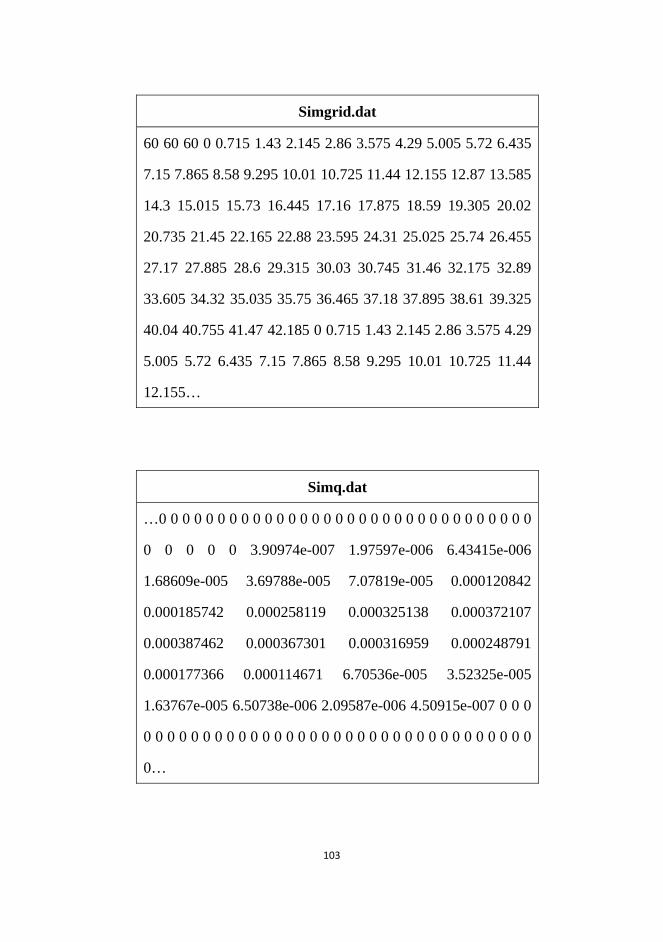
103  

Simgrid.dat

60 60 60 0 0.715 1.43 2.145 2.86 3.575 4.29 5.005 5.72 6.435

7.15 7.865 8.58 9.295 10.01 10.725 11.44 12.155 12.87 13.585

14.3 15.015 15.73 16.445 17.16 17.875 18.59 19.305 20.02

20.735 21.45 22.165 22.88 23.595 24.31 25.025 25.74 26.455

27.17 27.885 28.6 29.315 30.03 30.745 31.46 32.175 32.89

33.605 34.32 35.035 35.75 36.465 37.18 37.895 38.61 39.325

40.04 40.755 41.47 42.185 0 0.715 1.43 2.145 2.86 3.575 4.29

5.005 5.72 6.435 7.15 7.865 8.58 9.295 10.01 10.725 11.44

12.155…

Simq.dat

…0 0 0 0 0 0 0 0 0 0 0 0 0 0 0 0 0 0 0 0 0 0 0 0 0 0 0 0 0 0 0 0

0 0 0 0 0 3.90974e-007 1.97597e-006 6.43415e-006

1.68609e-005 3.69788e-005 7.07819e-005 0.000120842

0.000185742 0.000258119 0.000325138 0.000372107

0.000387462 0.000367301 0.000316959 0.000248791

0.000177366 0.000114671 6.70536e-005 3.52325e-005

1.63767e-005 6.50738e-006 2.09587e-006 4.50915e-007 0 0 0

0 0 0 0 0 0 0 0 0 0 0 0 0 0 0 0 0 0 0 0 0 0 0 0 0 0 0 0 0 0 0 0 0

0…

104  

11. Auxiliary rountines

None

12. Keywords

Phase-field parameter, homogeneous deformation

105  

Acknowledgements

I would like to express my deep thanks to Professor Rongshan, Qin and

Professor H.K.D.H. Bhadeshia for their supervision, encouragement and

help. And thanks to Professor Barlat, Frederic, Professor In Gee Kim and

Professor Suh, Dong-Woo for their great support, advice and friendship.

Thanks all the members in Computational Metallurgy Laboratory for

helping me so much. Their kindly help and great friendship will always on

my mind.

I am also appreciating Graduate Institute of Ferrous Technology and

POSCO for their financial support.

Finally, thanks to my parents for everlasting support for me.

106  

CURRICULUM VITAE

Name: Tan Xu (谭旭)

Date of birth: 9th, July 1984

Place of birth: GuiZhou Province, P.R. CHINA

Education:

M.S. POSTECH (Pohang, Korea), Graduate Institute of Ferrous

Technology, Computational Metallurgy.

B.S. 2007 Tsinghua University (Beijing, P. R. China), Engineering

Physics.