California State University, San Bernardino California State University, San Bernardino

CSUSB ScholarWorks CSUSB ScholarWorks

Electronic Theses, Projects, and Dissertations Office of Graduate Studies

3-2016

CLOTH - MODELING, DEFORMATION, AND SIMULATION CLOTH - MODELING, DEFORMATION, AND SIMULATION

Thanh Ho Computer Sciences

Follow this and additional works at: https://scholarworks.lib.csusb.edu/etd

Part of the Graphics and Human Computer Interfaces Commons

Recommended Citation Recommended Citation Ho, Thanh, "CLOTH - MODELING, DEFORMATION, AND SIMULATION" (2016). Electronic Theses, Projects, and Dissertations. 270. https://scholarworks.lib.csusb.edu/etd/270

This Project is brought to you for free and open access by the Office of Graduate Studies at CSUSB ScholarWorks. It has been accepted for inclusion in Electronic Theses, Projects, and Dissertations by an authorized administrator of CSUSB ScholarWorks. For more information, please contact scholarworks@csusb.edu.

CLOTH - MODELING, DEFORMATION, AND SIMULATION

A Project

Presented to the

Faculty of

California State University,

San Bernardino

In Partial Fulfillment

of the Requirements for the Degree

Master of Science

in

Computer Science

by

Thanh Ho

March 2016

CLOTH - MODELING, DEFORMATION, AND SIMULATION

A Project

Presented to the

Faculty of

California State University,

San Bernardino

by

Thanh Ho

March 2016

Approved by:

Dr. David Turner, Advisor, Computer Science & Engineering

Dr. Kerstin Voigt, Committee Member

Dr. Ernesto Gomez, Committee Member

© 2016 Thanh Ho

iii

ABSTRACT

This project presents the concepts of modeling cloth objects with different

materials by using parameters such as mass, stiffness, and damping. This

project also introduces deformation and simulation methods to present the

movement and interaction of cloth objects. The implementation is developed

using C++ for fast processing but the visualization is done by Maya, which is a

professional 3D modeling and animation tool.

iv

TABLE OF CONTENTS

ABSTRACT .......................................................................................................... iii

LIST OF FIGURES ...............................................................................................vi

CHAPTER ONE: INTRODUCTION ...................................................................... 1

CHAPTER TWO: RESEARCH TOOLS AND ENVIRONMENTS .......................... 2

CHAPTER THREE: PROJECT APPROACH

Modeling .................................................................................................... 3

Deformation ............................................................................................... 5

Simulation .................................................................................................. 8

CHAPTER FOUR: LIBRARIES AND TECHNIQUES

Vega .......................................................................................................... 9

TetGen ..................................................................................................... 10

Level Set 3 ............................................................................................... 11

Marching Cube/Square ............................................................................ 12

CHAPTER FIVE: IMPLEMENTATION

Overview Process .................................................................................... 17

Building the Distance Field Map .............................................................. 18

Building the Voxel Object ......................................................................... 20

Building Tetrahedrons and Mass-Spring System ..................................... 22

Building Marching Squares ...................................................................... 24

Object Deformation and Simulation ......................................................... 25

CHAPTER SIX: OBJECT MODELS AND RESULTS

Initial Flag ................................................................................................ 27

v

Flag with Two Fixed Corners ................................................................... 28

Flag Held at Center .................................................................................. 30

Flag Held on Vertical Edges .................................................................... 31

Flag with Horizontal Pole ......................................................................... 32

A Ball Falls Down into Flag ...................................................................... 34

Flag Held at Center By Pole .................................................................... 35

CHAPTER SEVEN: CONCLUSION ................................................................... 38

APPENDIX: SIMULATION EXPERIMENTS ....................................................... 39

REFERENCES ................................................................................................... 42

vi

LIST OF FIGURES

Figure 3.1. Simple model with vertices, edges and faces. .................................... 3

Figure 3.2. Voxel mesh. ........................................................................................ 4

Figure 3.3. Tetrahedral mesh. .............................................................................. 4

Figure 3.4. Mass-spring system (single voxel)...................................................... 6

Figure 3.5. Mass-spring system with force. .......................................................... 7

Figure 4.1. Tetrahedral mesh. ............................................................................ 10

Figure 4.2. Distance field map from Level Set 3. ................................................ 11

Figure 4.3. Marching cubes. ............................................................................... 12

Figure 4.4. Face with one vertex inside the mesh. ............................................. 13

Figure 4.5. 15 cases of marching cube ............................................................... 14

Figure 4.6. Marching squares with distance field. ............................................... 15

Figure 4.7. 16 cases of marching squares. ......................................................... 15

Figure 4.8. Marching squares in distance field map

(converted from 3D to 2D). .............................................................. 16

Figure 5.1. Implementation process. .................................................................. 17

Figure 5.2. Distance field map. ........................................................................... 19

Figure 5.3. Voxels with threshold 0. .................................................................... 20

Figure 5.4. Voxels with threshold 0.5. ................................................................. 21

Figure 5.5. Voxels covering the whole mesh in 3D view. .................................... 21

Figure 5.6. Tetrahedrons from a voxel. ............................................................... 22

Figure 5.7. Tetrahedral mesh. ............................................................................ 23

vii

Figure 5.8. Mass-spring system. ......................................................................... 23

Figure 5.9. Marching squares. ............................................................................ 24

Figure 5.10. Marching squares in 3D view ......................................................... 25

Figure 5.11. Marching squares with new position. .............................................. 26

Figure 5.12. Three frames of simulation ............................................................. 26

Figure 6.1. Initial flag mesh................................................................................. 27

Figure 6.2. Deformed flag with no applied forces ............................................... 28

Figure 6.3. Simulation of flag held at 2 corners .................................................. 29

Figure 6.4. Simulation of flag held at center ....................................................... 30

Figure 6.5. Simulation of flag held at left edge ................................................... 31

Figure 6.6. Observed motion of real flag held at edge ........................................ 32

Figure 6.7. Simulation of flag with pole (1) ......................................................... 33

Figure 6.8. Simulation of flag with pole (2) ......................................................... 34

Figure 6.9. Simulation of flag with dropping ball ................................................. 35

Figure 6.10. Simulation of flag held at center ..................................................... 36

Figure 6.11. Observed motion of real flag held at center .................................... 37

1

CHAPTER ONE

INTRODUCTION

This project addresses research challenges in modeling, deformation and

simulation of 3D cloth materials. These problems exist in the applied fields of

computer graphics, motion pictures, and movie animation. My project describes

and prototypes the process of simulating cloth using a mass-spring system to

control a deformable mesh. The processes of modeling, deforming, and

simulating are implemented in C++. The results are visualized using 3D

animation software, such as Maya and Blender.

2

CHAPTER TWO

RESEARCH TOOLS AND ENVIRONMENTS

There are two main tools used in this project. First, Visual Studio is used

to develop a library written in C++. Second, Maya is used as a host environment

for the C++ library.

Visual Studio provides the build environment needed to produce the

library to be loaded by Maya. Visual Studio makes sense for this project

because the development environment is a Windows-based computer. Visual

Studio provides excellent support for development and testing of the needed

library, including the ability to set break points, inspect variables and step through

the code. It also provides code assist functionality that makes it easier to

navigate the code base and avoid compilation errors due to incorrect spelling of

class and function names.

Maya is a widely used 3D modeling and animation tool. Maya is

extendable through a library plug-in architecture. This project makes use of this

extendibility by developing a library that lets animators apply algorithms and

methods in order to create, deform, and simulate models.

3

CHAPTER THREE

PROJECT APPROACH

Modeling

In this project, objects are presented by collections of vertices, edges, and

faces, which are commonly referred to as meshes (Figure 3.1). With these basic

elements, I can create functional models, such as voxel objects and tetrahedral

objects.

Figure 3.1. Simple model with vertices, edges and faces.

4

A voxel object represents an object using a set of cubes or 3D grid (Figure

3.2), and a tetrahedral object represents an object using a set of triangles (Figure

3.3).

Figure 3.2. Voxel mesh.

Figure 3.3. Tetrahedral mesh.

5

These functional models are useful (more formal) in applying techniques

to move or transform cloth models. These object models can be saved or

transferred easily in several formats, including OBJ, XML-based Collada, PLY or

FBX. In this project, however, I use our own text-based format to implement

these features.

The image in Figure 3.1 illustrates a simple model of a leaf that is

composed of vertices, edges and faces. It is converted into a set of voxels/cubes

(Figure 3.2). Then, it continues being converted to a tetrahedral mesh (Figure

3.3), which is a set of cubes where each cube is comprised of 6 triangles. This

process is described in detail in chapter 5.

Deformation

When a voxel or tetrahedral object is created from a normal mesh object, I

can use them to build a mass-spring system, which is a set of particles

connected by springs. (See Figure 3.4.) A mass-spring system relies on

properties of an object including: mass value per particle, spring stiffness,

damping coefficient, and rest length per spring.

6

Figure 3.4. Mass-spring system (single voxel).

Object deformation is the action of applying forces onto different points of

an object. Using a mass-spring system, I can find out the total force, including

both external and internal forces, which apply onto each particle and calculate

their new positions. For any two particles A and B (A = B + z), I have a spring AB

with rest length r and stiffness k. The spring force f can be calculated as follows:

f(z) = k(|z|-r)z/|z|.

Particle A receives a force f(z) and B receives a force –f(z). A change of

f(z) will cause a change of particle positions. Thus, I can deform the object by

providing or changing the forces between mesh vertices.

Face spring

Face diagonal spring

Body diagonal spring

7

Figure 3.5. Mass-spring system with force.

In Figure 3.5, a mass-spring system is represented by a wireframe

system. Each edge is a spring that holds stiffness values, and two vertices of that

edge hold mass values. A force is applied as shown by the yellow arrow in the

figure, which cause the springs representing the edges to stretch.

8

Simulation

By using different forces on different places of an object at different times

and adjusting values manually as needed, I can simulate objects with natural

motions or with special motions. By natural motion, I mean motion resulting from

only the application of gravity. By special motion, I mean motion resulting forces

other than gravity but possibly including gravity as well. An example of a natural

motion would be a flag falling down with only the force of gravity applied. An

example of a special motion would be pulling two corners of a flag by hand,

which would be simulated with forces at two corners of a flag. You can imagine

what this would look like if one held a flag by hand at two corners and stretched it

out. In general, the forces can result from many sources, such as gravity, wind,

and collisions with objects.

9

CHAPTER FOUR

LIBRARIES AND TECHNIQUES

Vega

Vega [2] is a C/C++ middleware library that includes many small libraries

that provide support for deformation and simulation of 3D objects.

The Vega library provides a mass-spring system; however, it is not

sufficient for generating natural looking motion in cloth. Although Vega uses an

object’s vertices and edges to directly build a mass-spring system, it cannot

conserve volume to keep the mesh stable. According to Diziol, Bender, and

Bayer [1], I can use voxel and tetrahedrons to build mass-spring volume

conservation systems in order to make a stable system. If I build a mass-spring

system directly from an object’s edges and vertices (Figure 3.1), the constraints

among edges and vertices are very weak and cannot fully represent material

characteristics. In voxel and tetrahedral systems (Figure 4.1), constraints are

more stable because of the connections inside and among the voxels and

tetrahedrons.

Using different values of mass, damping and stiffness in the Vega mass-

spring system, a mesh can be used to simulate various kinds of materials.

10

TetGen

TetGen [3] is a C/C++ library that provides support for building a

tetrahedral mesh (Figure 4.1) using Voronoi partition techniques. One Voronoi

technique is to partition a planar surface with n points into convex polygons such

that each polygon contains exactly one generating point and every point in a

given polygon is closer to its generating point than to any other [4]. Another

technique uses a Voronoi partition with Delaunay triangulation, which is

equivalent to the nerve of the cells in a Voronoi diagram [5]. In our case, because

the mesh is converted into voxels/cubes by a software process called a voxelizer,

they can be used as Voronoi partitions. The tetrahedral parts can be treated

similarly.

Figure 4.1. Tetrahedral mesh.

11

Level Set 3

Level Set 3 is a part of the El Topo library. I use this library to build a

distance field map of a mesh in either 3D or 2D. A distance field map is a map of

points that show distances from each point to closest points on the mesh (Figure

4.2). A positive distance value means that the point is outside the mesh and a

negative distance value means the point is inside the mesh. A more detailed map

is used to represent a higher quality mesh. I use a distance field to create voxels

and marching cubes (3D) or marching squares (2D), which will be used in the

simulation as explained in the next section.

Figure 4.2. Distance field map from Level Set 3.

12

Marching Cube/Square

Marching cubes is a technique for rebuilding a mesh from a distance field

map. In Figure 4.3, the green lines represent the edges of the mesh and the blue

lines represent the edges of the marching cubes, which are used to deform the

mesh.

Figure 4.3. Marching cubes.

13

The marching cubes are formed from the points on the distance field. For

each cube, I create a polygon from the data in the distance field, as explained

below. When going through the marching cubes, I consider cubes that have both

positive and negative values. Those cases indicate whether the cube has

vertices inside the mesh (when the point has a negative distance value) and

outside the mesh (when the point has a positive distance value). When a cube

has vertices both inside and outside a mesh, then the cube intersects the mesh,

defining a face within the mesh (Figure 4.4). The edges which have one vertex

(A) inside the mesh and one vertex (B) outside the mesh should intersect the

mesh at a point on the line (AB). From the combination of all intersection vertices

in the cube, I can rebuild a face (triangle or rectangle) for the marching mesh.

Figure 4.4. Face with one vertex inside the mesh.

Isosurface

0.8

-0.15

0.6 0.5

0.5

0.6

0.5

0.6

14

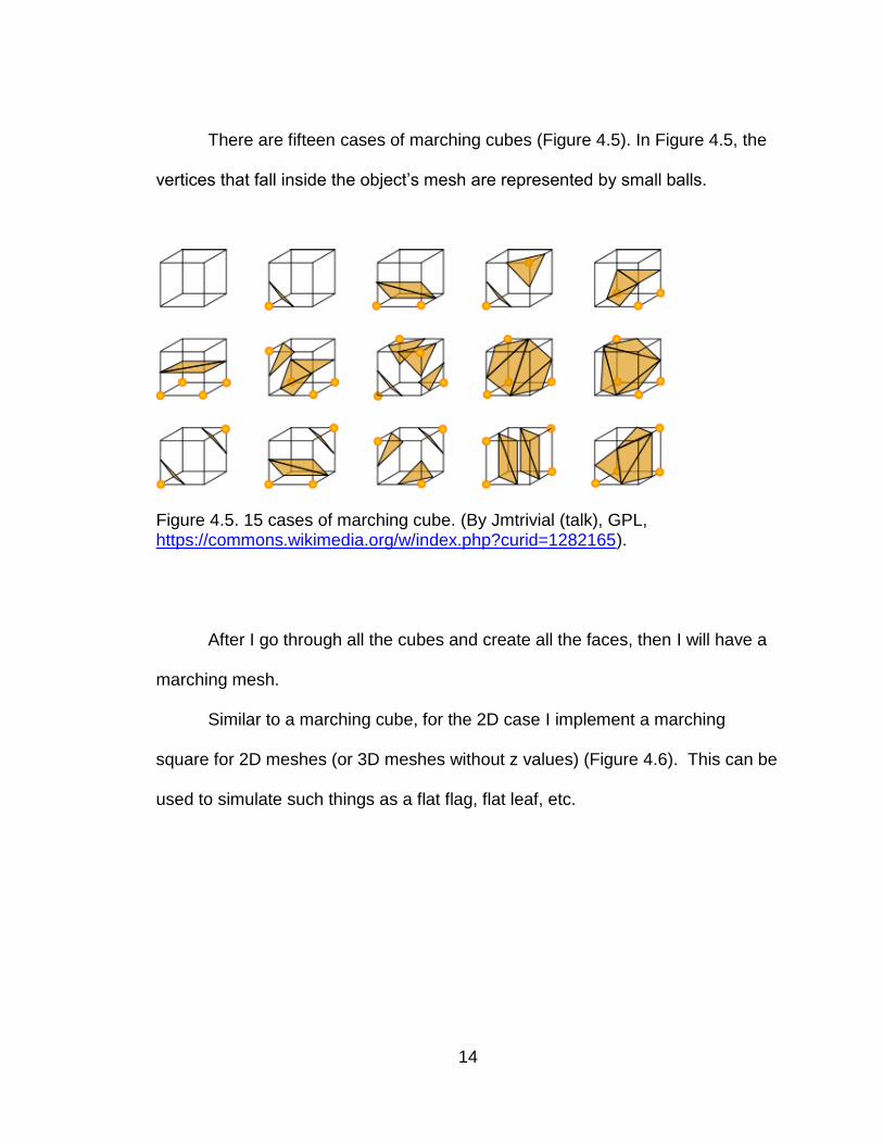
There are fifteen cases of marching cubes (Figure 4.5). In Figure 4.5, the

vertices that fall inside the object’s mesh are represented by small balls.

Figure 4.5. 15 cases of marching cube. (By Jmtrivial (talk), GPL, https://commons.wikimedia.org/w/index.php?curid=1282165).

After I go through all the cubes and create all the faces, then I will have a

marching mesh.

Similar to a marching cube, for the 2D case I implement a marching

square for 2D meshes (or 3D meshes without z values) (Figure 4.6). This can be

used to simulate such things as a flat flag, flat leaf, etc.

15

Figure 4.6. Marching squares with distance field.

For the 2D case, I have sixteen cases of marching squares used to

determine how an edge is created in the marching square (Figure 4.7).

Figure 4.7. 16 cases of marching squares.

0.5

0.707 0.5

-0.354

16

Figure 4.8 shows a corner of a marching mesh built from a distance field

map in 2D.

Figure 4.8. Marching squares in distance field map (converted from 3D to 2D).

17

CHAPTER FIVE

IMPLEMENTATION

Overview Process

An overview of the implementation process is shown in Figure 5.1.

Figure 5.1. Implementation process.

Mesh

Build

distance

field

Distance

field map

Voxelizer Voxels Tetrahedralize

Tetrahedral Build mass-

spring

system

Mass-spring

system

Deforming

Simulating Deform

mesh

Start

End

18

The process starts with the input of a 2D mesh (in a 3D coordinate

system). Its vertices and edges will be passed to the Level Set 3 library in order

to build a distance field map. Then the voxelizer uses the map values to build a

voxel system in which each voxel should be either inside or on the face of a

mesh. Each voxel is then divided into 6 tetrahedrons. After a tetrahedral mesh is

built from all the voxels, its vertices and edges are used as a mass-spring

system. Providing various initial stiffness and mass values for the mass-spring

system, I can represent various kinds of materials. Applying constant or

adjustable forces during a period of time, I can deform and simulate the mesh.

Building the Distance Field Map

Using the Level Set 3 library, I provide all vertices and faces to get a

distance field map (Figure 5.2). I limit how big the map is so that the object’s

mesh falls completely within the map at its initial position and at all subsequent

positions as a result of simulating its motion.

19

Figure 5.2. Distance field map.

In almost cases, the distance between two points of the map, called voxel

width, is 1 unit of length. With a smaller voxel width, the distance field map will

have more detail. However, it will take more time to process more values from

the map. Also, a more detailed mesh (which renders a higher quality image of the

object) needs more time to process. Thus, adjusting voxel width to get a

reasonable performance is necessary.

20

Building the Voxel Object

After the distance field map is calculated, I can build voxels for the map.

Each point in the distance field map shows how far the point is from the mesh

and, by the sign of the value, whether the point is inside or outside mesh. Points

that are inside or on the surface of the mesh are chosen to create voxels.

In theory, I use positive and negative values to check if a voxel is created

(threshold is 0). But when implemented, there is a lot of cases where a positive

value is near to zero. This occurs when the point is very close to the mesh

surface. In this case, the voxels cannot cover the whole mesh (Figure 5.3).

Figure 5.3. Voxels with threshold 0.

Mesh

Voxel (distance field is -0.15)

Close point (distance field is 0.1)

21

In my implementation, I do a lot of experiments and then decided to

choose threshold values about a half of the voxel width, which is the distance

between neighboring points in the distance field map. In most of the cases,

voxels will cover the whole mesh (Figures 5.4 and 5.5).

Figure 5.4. Voxels with threshold 0.5.

Figure 5.5. Voxels covering the whole mesh in 3D view.

Voxel (distance field is 0.1) Mesh

Voxel (distance field is -0.15)

22

Building Tetrahedrons and Mass-Spring System

Tetrahedrons are built from voxels by dividing each voxel into six

tetrahedrons, which is illustrated in Figure 5.6. Each tetrahedralized voxel has 8

vertices and 9 edges.

Figure 5.6. Tetrahedrons from a voxel.

I build a tetrahedral mesh by converting all voxels to tetrahedrons (Figure

5.7). The set of vertices and edges of the tetrahedral mesh comprise the mass-

spring system (Figure 5.8). I assign mass values to vertices and stiffness values

to edges to represent various materials. These values are adjusted to get a good

simulation.

23

Figure 5.7. Tetrahedral mesh.

Figure 5.8. Mass-spring system.

24

Building Marching Squares

From a distance field map, I build a marching square mesh. Figure 5.9

shows a marching mesh built from 2D distance field map. Each four closest

points form a square, so I go through all squares in the distance field map to

generate the marching squares. (See the section on marching cubes/squares in

Chapter 4.)

Figure 5.9. Marching squares.

Because I want to build a model in 3D, I implement marching squares in

3D in which each square becomes a cube (Figure 5.10). In 3D, two points on the

same z-index are considered as 1 point in 2D mode. Thus, I can easily convert

25

between 3D and 2D modes. This may also be considered as a special case of

marching cubes.

Figure 5.10. Marching squares in 3D view

Object Deformation and Simulation

I have a relationship between the distance field map and the mass-spring

system, where each point in the distance field map refers to one voxel and also 8

points of the mass-spring system. When I provide forces onto a mass-spring

system to make it move, the vertices in the mass-spring system take on new

positions. I will apply these new positions onto the distance field map using the

relationship between them. Then I perform marching squares with the initial

values of the distance field map (which do not change with time) and combine

this with the new positions. See Figure 5.11 for an example.

26

Figure 5.11. Marching squares with new position.

The simulation is computed for successive points in time by deforming the

mesh for each small interval of time. Figure 5.12) shows how this might look for 3

separate times in the simulation. These points in time are referred to as frames

in animation tools such as Maya. I can adjust the force per time period (specified

in seconds or frames) to find out the way to simulate a mesh naturally (includes

gravity force only), or specially (includes forces other than gravity).

Figure 5.12. Three frames of simulation

27

CHAPTER SIX

OBJECT MODELS AND RESULTS

Initial Flag

In this chapter I consider the problem of simulating the movement of a

flag. The example flag I consider is a 10 by 6 grid of cubes (Figure 6.1). Its mass

is 10 kilograms per meter cubed (kg/m3). Its stiffness values (called Young’s

Modulus) are 20000, 100, and 100 newtons per meter squared (N/m2) for face

spring, face diagonal spring, and body diagonal spring (See section on

Deformation of Chapter 3).

Figure 6.1. Initial flag mesh.

28

Figure 6.2 shows the flag deformed by running the simulation without user

force and gravity.

Figure 6.2. Deformed flag with no applied forces

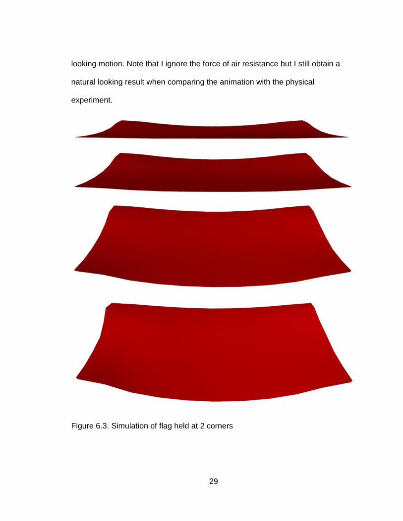
Flag with Two Fixed Corners

The first experiment that I consider is holding a flag at two corners and

letting it fall freely. Considering gravity as the only force, I have: fy = -9.8N,

where f represents the force in the y direction. Figure 6.3 contains 3 frames of

the resulting simulation. Based on performing the actual physical experiment

with a real flag, I conclude that this process is sufficient for producing a natural

29

looking motion. Note that I ignore the force of air resistance but I still obtain a

natural looking result when comparing the animation with the physical

experiment.

Figure 6.3. Simulation of flag held at 2 corners

30

Flag Held at Center

In this experiment, I hold the flag at its center and blow on its left edge as

it falls from a horizontal position. In this case, I have the force of gravity: fy = -

9.8N. But I also have the user’s blowing force: fx = 15N and fy = -15N.

Figure 6.4 contains 2 frames of the resulting simulation. I did not perform

a physical experiment with a real flag; instead, I use subsequent simulations and

experiments to build our confidence that our simulation is natural looking.

Figure 6.4. Simulation of flag held at center

31

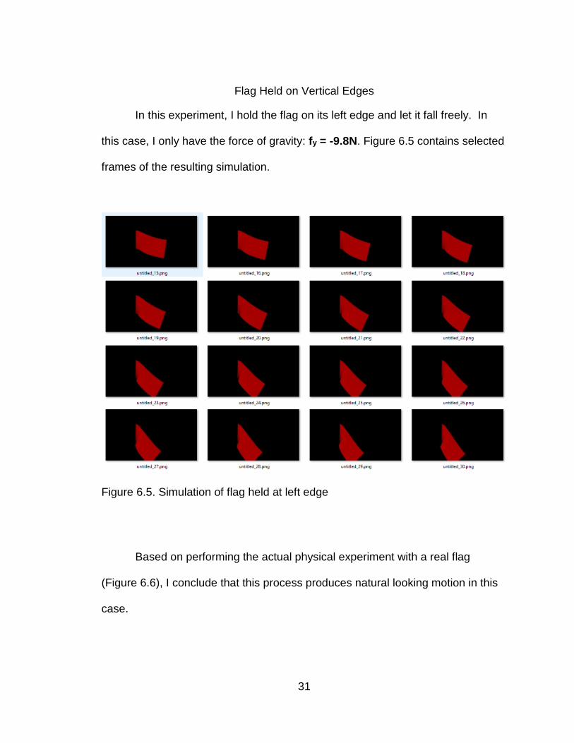
Flag Held on Vertical Edges

In this experiment, I hold the flag on its left edge and let it fall freely. In

this case, I only have the force of gravity: fy = -9.8N. Figure 6.5 contains selected

frames of the resulting simulation.

Figure 6.5. Simulation of flag held at left edge

Based on performing the actual physical experiment with a real flag

(Figure 6.6), I conclude that this process produces natural looking motion in this

case.

32

Figure 6.6. Observed motion of real flag held at edge

Flag with Horizontal Pole

This experiment is done with flag and pole. An edge of the flag is attached

to a pole. The two opposite corners are held by hand initially. The pole is kept in

a horizontal position throughout the entire experiment. The flag is initially

positioned flat in a horizontal position. I then release the two hand held edges of

the flag and observe its falling motion. The force of gravity will be the only

external force involved: fy = -9.8N. Figure 6.7 contains 2 frames of the resulting

animation. The simulated result resembles the actual motion when performing

the experiment with a real flag.

33

Figure 6.7. Simulation of flag with pole (1)

I extend the problem to include a wind force in addition to the gravity force.

In particular, I apply a wind force at middle of the flag with: uy = 30N for a line

passing through the center and uy = 0 for all other points. The total force is the

force of gravity plus the user force: fy + uy, where fy is the force due to gravity.

Figure 6.8 contains 2 frames of the resulting simulation. I did not perform a

physical experiment for this problem.

34

Figure 6.8. Simulation of flag with pole (2)

A Ball Falls Down into Flag

In this experiment, I drop a ball into the middle of the flag without gravity

affecting the flag. The force that the ball applies onto middle point of flag is

represented as: fy = -50N for the center point and fy = 0 for all other points.

Figure 6.9 contains 2 frames of the resulting animation. I did not perform a

physical experiment for this problem.

35

Figure 6.9. Simulation of flag with dropping ball

Flag Held at Center By Pole

In this experiment, I hold the flag at center point and let it fall freely. In this

case, I only have the force of gravity: fy = -9.8N. Figure 6.10 contains selected

frames of the resulting simulation.

36

Figure 6.10. Simulation of flag held at center

37

Based on performing the actual physical experiment with a real flag

(Figure 6.11), I conclude that this process produces natural looking motion in this

case.

Figure 6.11. Observed motion of real flag held at center

38

CHAPTER SEVEN

CONCLUSION

In general, this project aims to understand realistic animation processing

and to improve and extend current methods for better performance. Cloth

material is common in real life, so the realism of the simulated cloth motion can

be checked through visual inspection. Once the basic simulation techniques are

validated with actual physical experiments, I can use those techniques to

produce animations that appear natural. This project has determined several

such techniques that can now be used for applied cloth animation problems. In

future work, I can extend the concepts to the simulation of plastic, wood, steel

and other materials.

39

APPENDIX

SIMULATION EXPERIMENTS

40

The following animation frames were generated from the simulation of a

falling flag held on left edge.

41

The following animation frames were generated from the simulation of a

falling flag held in its center.

42

REFERENCES

[1] R. Diziol, J. Bender, and D. Bayer, “Volume conserving simulation of

deformable bodies,” in Proceedings of Eurographics 2009, Munich,

Germany, 2009.

[2] J. Barbič, F. S. Sin, and D. Schroeder, “Vega: Non-Linear FEM

Deformable Object Simulator,” Computer Graphics Forum, vol. 32, pp. 38-

50, 2013.

[3] H. Si. (2013, November). TetGen. [Online]. Available: http://wias-

berlin.de/software/tetgen/tetview.html

[4] E. W. Weisstein, "Voronoi Diagram," [Online]. Available:

http://mathworld.wolfram.com/VoronoiDiagram.html. [Accessed 1

November 2015].

[5] E. W. Weisstein, "Delaunay Triangulation," [Online]. Available:

http://mathworld.wolfram.com/ DelaunayTriangulation.html. [Accessed 1

November 2015].