Perturbation equations for all-scale

atmospheric dynamics

Piotr K. Smolarkiewicz a, Christian Kuhnlein a, Nils P. Wedi a

aEuropean Centre For Medium-Range Weather Forecasts, Reading, RG2 9AX, UK

Abstract

This paper presents generalised perturbation forms of the nonhydrostatic partialdifferential equations (PDEs) that govern dynamics of all-scale global atmosphericflows. There can be many alternative perturbation forms for any given system of thegoverning PDEs, depending on the assumed ambient state about which perturba-tions are taken and on subject preferences in the numerical model design. All suchforms are mathematically equivalent, yet they have different implications for thedesign and accuracy of effective semi-implicit numerical integrators of the govern-ing PDEs. Practical and relevant arguments are presented in favour of perturbationforms based on the solutions’ computational efficacy. The optional forms are im-plemented in the high-performance finite-volume module (IFS-FVM) for simulatingglobal all-scale atmospheric flows [Smolarkiewicz et al., J. Comput. Phys. (2016)doi:10.1016/j.jcp.2016.03.015]. The implementation of the general and flexible per-turbation formulation is illustrated and verified with a class of ambient states ofreduced complexity. A series of numerical simulations of the planetary baroclinicinstability, epitomising global weather, illustrates the accuracy of the perturbationequations. The novel numerical approach has the potential for numerically accurateseparation of a background state from finite-amplitude perturbations of the globalatmosphere. Practical implications include far less sensitivity to grid imprintingon non-uniform meshes, undiluted interaction of background shear with rotationalmotions, and an improved accuracy and reliability of extended-range predictions.

Key words: atmospheric models, flexible PDEs, nonoscillatory forward-in-timeschemes, numerical weather prediction, climatePACS:

∗ Corresponding Author.Email address: smolar@ecmwf.int (Piotr K. Smolarkiewicz).

Preprint submitted to J. Comput. Phys. 10 April 2018

1 INTRODUCTION

An important characteristic of the atmospheric dynamics is that it constitutesa relatively small perturbation about dominant hydrostatic and geostrophicbalances established in effect of the Earth gravity, rotation, stably-stratifiedthermal structure of its atmosphere and the energy provided by the incomingflux of solar radiation. For illustration, consider that the total conversion ofavailable potential energy to kinetic energy in the global atmosphere is only0.26% of the incoming solar radiation at the top of the atmosphere; cf. Fig. 1in [46]. Preserving this fundamental equilibrium, while accurately resolvingthe perturbations about it, conditions the design of atmospheric models andsubjects their numerical procedures to intricate stability and accuracy re-quirements. In particular, extended-range (11-45 days) and seasonal weatherpredictions (up to 1 year ahead) are subjected to dominant initial and modelbiases in the simulation of the atmosphere/ocean and suffer from low signal-to-noise ratios. In seasonal forecasting, this proofs a difficult problem for thedetection of anomalies, especially when there is also a model drift relative tolong-term biases in the simulated quantities [20]. The conceptual idea of theapproach implemented in this paper is a numerically accurate separation anddual evolution of an arbitrary (but advantageously selected) ambient stateand finite-amplitude perturbations around this state, to improve conservationproperties, mean state bias and drift, and the reliability of extended-rangepredictions.

Given the nature of atmospheric dynamics, it is compelling to formulate gov-erning PDEs in terms of perturbation variables about an arbitrary state ofthe atmosphere that already satisfies some or all of the dominant balances. Infact, this is a standard approach in small-scale atmospheric modelling basedon soundproof equations, such as the classical incompressible Boussinesq sys-tem or its anelastic or pseudo-incompressible generalisations. The key role ofthe reference state in these equation systems is to uncouple a dominating hy-drostatic balance from buoyancy driven motions, and to justify linearisationsrequired to achieve a physically-relevant complexity reduction. Otherwise, thereference state does not have to be unique nor represent the actual mean stateof the system. The primary strength of established reference states is theirgenerally recognized theoretical and practical validity. However, such refer-ence states are overly limited, most often consisting only of a single stablyor neutrally stratified vertical profile of thermodynamic variables. To allevi-ate this limitation, soundproof models often account for an additional, moregeneral balanced state, hereafter referred to as an “ambient” state [27].

The notion of ambient states is distinct from that of the reference state. Theutilization of an ambient state is justified by expediency and optional for anysystem of the governing equations. The role of ambient states is to enhance the

2

efficacy of numerical simulation—e.g. by simplifying the design of the initialand boundary conditions and/or improving the conditioning of elliptic bound-ary value problems—without resorting to linearisation of the system. The keyunderlying assumption is that the ambient state is a particular solution of thegoverning problem, so that subtracting its own minimal set of PDEs from thegoverning equations can provide a useful perturbation form of the governingsystem. In general, ambient states are not limited to stable or neutral stratifi-cations [8], can be spatially and temporally varying to represent, e.g. thermallybalanced large-scale steady flows in atmospheric models [26,35] or prescribeoceanic tidal motions [39]. Here, we present a generalised formalism allowing,in principle, for an arbitrary (yet advantageous) ambient state. In the contextof this development, it is hoped that there are special cases of such arbitrarystates that can be particularly useful for weather and climate applications.All theoretical developments directly pertain to two advanced all-scale mod-elling systems, the Eulerian-Lagrangian (EULAG) research model for multi-scale flows [23,34,35] and the Finite-Volume Module (IFS-FVM) [36,13,37] inthe Integrated Forecasting System (IFS) of the European Centre for Medium-Range Weather Forecasts (ECMWF).

The paper is organised as follows: Section 2 derives the perturbation form ofthe nonhydrostatic compressible Euler equations of all-scale atmospheric dy-namics. The related numerical procedures are described in Section 3. Section 4substantiates technical developments of the preceding sections, with a seriesof simulations of the planetary baroclinic instability. Section 5 concludes thepaper.

2 GOVERNING EQUATIONS

2.1 Generic form

The generalised PDEs of EULAG [35] and IFS-FVM [36] assume the com-pressible Euler equations under gravity on a rotating sphere as default, butinclude reduced soundproof equations [18,6] as options. From the perspectiveof numerics, the design of the semi-implicit integrators in FVM follows thesame path for the compressible and the anelastic system. Hence, we focus onthe most general case of the compressible Euler equations. For simplicity, westart the presentation with the physically more intuitive advective form ofthe inviscid governing equations formulated on a rotating sphere, and intro-duce the corresponding conservation forms implemented in FVM afterwards inSection 3. With these caveats, the advective forms of equations for density ρ,potential temperature θ and the physical velocity vector u can be compactly

3

written as

dρ

dt= − ρG∇ · (Gv) , (1a)

dθ

dt= H , (1b)

du

dt= − θ

θ0G∇φ+ g − f × u +MMM(u) + DDD(u) . (1c)

Here, d/dt = ∂/∂t+ v · ∇, with ∇ = (∂x, ∂y, ∂z) representing a vector of spa-tial partial derivatives with respect to the generalised curvilinear coordinatesx = (x, y, z) [22,42,11] (assumed stationary for the purpose of this paper) andv = GTu, where G denotes a 3× 3 matrix of known metric coefficients. Fur-thermore, G symbolises the Jacobian—i.e. the square root of the determinantof the metric tensor—whereas f and MMM(u) respectively mark the vectors ofCoriolis parameter and metric forcings (i.e., Christoffel terms) shown for aplain geospherical framework in Appendix A. In (1b), H symbolises a heatsource/sink, including diffusion. In (1c), g is the vector of gravitational accel-eration, while DDD(u) symbolises momentum dissipation. The pressure variableφ = cpθ0π renormalises the Exner-function of pressure, π := (p/p0)

R/cp = T/θ,upon which it satisfies the gas law

φ = cpθ0

(Rp0ρθ

)R/cv . (2)

Here, cp and cv denote specific heats at constant pressure and volume, respec-tively, R is a gas constant, T indicates the temperature, and subscripts “0”refer to constant reference values.

2.2 Ambient state

We now assume an arbitrary ambient state (ρa, θa, φa,ua) that satisfies thesame generic form of the governing equations, or a subset thereof,

daρadt

= −ρaG∇ · Gva , (3a)

daθadt

= Ha , (3b)

dauadt

= −θaθ0

G∇φa + g − f × ua +MMM(ua) + DDD(ua) , (3c)

4

where da/dt = ∂/∂t + va · ∇ with va = GTua. Correspondingly, the ambientpressure variable φa = cpθ0πa satisfies

φa = cpθ0

(Rp0ρaθa

)R/cv , (4)

2.3 Perturbation forms

2.3.1 Derivation

In order to derive perturbation forms of the governing equations (1b) and (1c),the perturbation dependent variables are first defined as

θ′ := θ − θa , u′ := u− ua , φ′ := φ− φa . (5)

Second, the two auxiliary relations are derived:

∀ ψ = ψ′ + ψa ,dψ

dt− daψa

dt≡ dψ′

dt+ v′ · ∇ψa ; (6a)

θ

θ0G∇φ− θa

θ0G∇φa ≡

θ

θ0G∇φ′ + θ′

θ0G∇φa . (6b)

Then subtracting (3b) from (1b) and (3c) from (1c), and rearranging the termswhile using (6a) and (6b), leads to the perturbation forms

dθ′

dt= −v′ · ∇θa +H′ , (7a)

du′

dt= −v′ · ∇ua −

θ

θ0G∇φ′ − θ′

θ0G∇φa

− f × u′ +MMM′(u′,ua) + DDD ′(u′,ua) ,(7b)

where

H′ = H−Ha ,

v′ = GTu′ ,

MMM′(u′,ua) =MMM(u′ + ua)−MMM(ua) ,

DDD ′(u′,ua) = DDD(u′ + ua)− DDD(ua) ,

(8)

the last of which reduces to DDD ′ = DDD(u′) for a solution-independent viscosity.

Among the two perturbation equations in (7), the entropy equation (7a) isstraightforward to interpret. The corresponding (specific) momentum equation(7b) is revealing, in that it reduces a total of all ambient forcings into a

5

generalised 3D buoyancy term relating to θ′∇φa on the rhs. This can be seenreadily when representing G∇φa in terms of (3c) as

G∇φa =θ0θa

(g − f × ua +MMM(ua) + DDD(ua)−

dauadt

). (9)

Importantly, substituting (9) in (7b) and manipulating the terms—such as toseparate the gravitational, inertial and dissipative forcings on the rhs—leadsto an alternative perturbation form of the momentum equation

du′

dt=− v′ · ∇ua −

θ

θ0G∇φ′ − g

θ′

θa− f ×

(u− θ

θaua

)

+

(MMM(u)− θ

θaMMM(ua)

)+

(DDD(u)− θ

θaDDD(ua)

)+θ′

θa

dauadt

,

(10)

where u = u′ + ua is utilised on the rhs. Furthermore, moving the first termon the rhs of (10) to the lhs, then using (6a) and then moving dua/dt back tothe rhs to combine it with the last term, produces

du

dt=− θ

θ0G∇φ′ − g

θ′

θa− f ×

(u− θ

θaua

)

+

(MMM(u)− θ

θaMMM(ua)

)+

(DDD(u)− θ

θaDDD(ua)

)+

θ

θa

dauadt

.

(11)

The latter form is already familiar from [35,36]—cf. eqs. (39) and (1c), respec-tively, in [35] and [36]—where it was used for the special case of the thermallybalanced zonal wind (inviscid) in (3) implying daua/dt ≡ 0 and DDD(ua) ≡ 0 onthe lhs and rhs of (3c), respectively. Moreover, the process of navigating from(7b) to (11) suggests yet another form

du

dt=− θ

θ0G∇φ′ − θ′

θ0G∇φa − f × (u− ua)

+ (MMM(u)−MMM(ua)) + (DDD(u)− DDD(ua)) +dauadt

,

(12)

a variant of (11) formulated in terms of the generalised buoyancy or, alter-natively, a variant of (7b) formulated in terms of full velocity rather than itsperturbations.

2.3.2 Discussion

The four perturbation forms of the momentum equation (7b), (10), (11) and(12) are mathematically equivalent, as their derivations only manipulate se-lected terms in the equations and redefine dependent variables. From the per-spective of numerical approximations, however, different forms enable novel

6

algorithmic designs, with (7b) promising greater efficacy, especially in the con-text of “long or fussy integrations” [19]. Because of the aforementioned speci-ficity of global atmospheric flows, our focus is on two-time-level nonoscillatoryforward-in-time (NFT) integrators, implicit with respect to acoustic, buoyant,and rotational modes. At the highest level, the NFT template represents theproblem solution as a sum of explicit and implicit terms,

ψψψn+1i = Ai

(ψψψn+0.5δtRRR(ψψψn)

)+0.5δtRRRi(ψψψ

n+1) ≡ ψψψ i +0.5δtRRRi(ψψψn+1) (13)

where ψψψ symbolises the vector of dependent variables (u, θ, φ, ρ) or pertur-bations thereof, n and i refer to the temporal and spatial position on a dis-cretisation mesh, A symbolises a NFT advective transport operator, and RRRmarks the cumulative forcings on the rhs of the PDE system at hand. Thetemplate (13) is common for both the advective ( dψψψ/dt = RRR ) and the con-servative ( ∂Gρψψψ/∂t + ∇ · Gρvψψψ = GρRRR ) forms of the governing equations.In the former case, (13) represents a class of trajectory-wise semi-Lagrangianintegrators, whereas in the latter case it refers to a class of control-volume-wise Eulerian integrators. Generally, RRR is composed of linear and nonlinearcomplements in terms of ψψψ. The nonlinear elements are explicitly predictedat n + 1, upon which all linear terms are treated implicitly. This class ofalgorithms—widely-documented in the literature, see [35,36] and referencestherein—benefits both computational stability and accuracy of discrete inte-grations. In particular, the adopted trapezoidal-rule integration of all restor-ing forces is free of amplitude errors, which is especially important for rep-resenting slow oscillations and wave phenomena in geo/astrophysical systems[43,4,32,45,8,24], and different perturbation forms encourage different level ofimplicitness in determining final solutions for ψψψn+1.

Among (7b), (10), (11) and (12), (7b) implies integrators with the highest de-gree of implicitness as, except for the coefficient of the pressure gradient andthe metric forcing, the remaining rhs can be viewed as an action of a linearoperator on the vector of the perturbation variables (u′, φ′, θ′). There are twonoteworthy aspects of (7b). One is the convective derivative of the ambientvelocity component analogous to the convective derivative of the ambient po-tential temperature in (7a). The other is the vectorial buoyancy term, ∝ θ′,appearing in all three components of the momentum equation. This contrastswith (11), familiar from solving implicitly for the full velocity with buoyancystandardly confined to the vertical (viz. radial on the sphere) component equa-tion aligned with g. Furthermore, all coefficients θ/θa on the rhs of (11) arepredicted explicitly at tn+1. The form (10) is intermediate between (7b) and(11), in that it retains many aspects of the familiar design while still solving forthe velocity perturbations. Conversely, (12) retains the generalised buoyancyof (7b) while solving for the full velocity. The ability of solving all four formsis useful for assessing the relative importance of various terms and balancesin numerical integrations. In the following, we shall focus on the complete de-

7

scription of (7b), as it appears the most promising in terms of computationalefficacy and implementation flexibility while revealing the most challengingelliptic Helmholtz problem associated with the implicit integration procedure.Furthermore, having an effective integrator for (7b) enables incorporation ofthe other three options in the same model code with relative ease.

3 NUMERICAL APPROXIMATIONS

3.1 Semi-implicit integrators

The system of PDEs based on (1a), (7a) and (7b) is cast in the conservationform

∂Gρ∂t

+∇ · (Gρv) = 0 , (14a)

∂Gρθ′

∂t+∇ · (Gρvθ′) = −Gρ

(GTu′ · ∇θa −H′ − αθθ′

), (14b)

∂Gρu′

∂t+∇ · (Gρv ⊗ u′) =− Gρ

(GTu′ · ∇ua +

θ

θ0G∇φ′ + θ′

θ0G∇φa

+ f × u′ −MMM′(u,ua)− DDD ′(u,ua)− αuu′),

(14c)

and consistently augmented with the relaxation terms −αθθ′ and −αuu′ in theentropy and momentum equation, respectively. These numerical devices sim-ulate, e.g. wave absorbing devices in the vicinity of the open boundaries [27]and/or immersed solids [31], or provide a basic tool for time-continuous dataassimilation [3]. The coefficients αθ and αu—generally, functions of (x, t)—represent inverse time-scales for the relaxation of actual potential temperatureand velocity fields towards their ambient values. Although numerically moti-vated, these devices are treated consistently with physical forcings and needto be rigorously accounted for in the construction of semi-implicit integrators;cf. Appendix A in [22].

The semi-implicit integrator of the system (14) adopts the general NFT tem-plate (13) following the procedure detailed in [35,36]. This procedure com-mences with integration of the mass continuity equation (14a) as

ρn+1i = Ai

(ρn, (vG)n+1/2 ,Gn,Gn+1

)=⇒ Vn+1/2 = v⊥Gρn+1/2

(15)

where A denotes a bespoke multidimensional positive definite advection trans-port algorithm (MPDATA) for compressible atmospheric flows [13], a hybrid[36] of structured-grid [30] and unstructured-mesh [29] schemes for the verti-cal and horizontal discretisations. Given the provision of a first-order accurate

8

estimate of the advector (vG)n+1/2 at the intermediate time level tn+1/2, Ai

provides a second-order accurate solution for ρn+1i ∀ i, together with the cumu-

lative face-normal advective mass fluxes Vn+1/2. These advective mass fluxesand the updated density ρn+1 are subsequently applied in the integration of(14b) and (14c) following (13). Namely,

θ′n+1i = θ′i − 0.5δt

(GTu′

n+1 · ∇θn+1a + αθθ′

n+1)i

(16a)

u′n+1i = u′i − 0.5δt

(GTu′

n+1 · ∇un+1a

)i

− 0.5δt

(θ?

θ0G∇φ′ n+1

+θ′ n+1

θ0G∇φn+1

a

)i

− 0.5δt(f × u′

n+1 −MMM′(u′?,un+1

a ) + αuu′n+1

)i,

(16b)

where:

θ′i = Ai

(θ′,Vn+1/2, (ρG)n, (ρG)n+1

), θ′ =

(θ′ + 0.5δtRθ

)n; (17a)

u′i = Ai

(u′,Vn+1/2, (ρG)n, (ρG)n+1

), u′ = (u′ + 0.5δtRRRu)

n; (17b)

and where superscript ? on the rhs of (16b) refers to explicit predictors exe-cuted iteratively and lagged behind the linear terms; see section 3.2 in [36].Furthermore, the perturbation heat source H′ has been included in the θ′ ar-gument of the transport operator, by adopting the Rθ = GTu′ · ∇θa + 2H′representation at tn. Analogously, RRRu subsumes the perturbation dissipationterm 2DDD ′.

The integrator outlined in (16) contains fully implicit trapezoidal integrals ofgeneralised buoyancy, Coriolis and relaxation terms, whereas trapezoidal in-tegrals of the nonlinear terms of pressure-gradient and metric forcings employexplicit predictors of full potential temperature and velocity, respectively. Thederivation of the closed-form expression for the velocity update is involving.The overall idea is to substitute the potential temperature in the generalisedbuoyancy term of (16b) with the rhs of the entropy integral (16a) and gather allterms depending on un+1 on the lhs of the momentum integral, upon which theclosed-form expression for velocity update emerges as an inversion of a linearproblem. To simplify the notation, in the following the spatial position indexi is dropped everywhere, as all dependent variables, coefficients and terms areco-located in (16). Similarly, the temporal index n + 1 is also dropped, asthere is no ambiguity. Furthermore, the ratios of the potential temperatureand its reference value are subsequently referred to as θ/θ0 = Θ, whereasδht = 0.5δt. Because further derivations require an intricate component repre-sentation of the vector equation (16b), we adopt the notations u = (ux, uy, uz)

9

and G∇ = ∇ = (∂x, ∂y, ∂z).1 We also note the auxiliary relation

∀ ψ, (GTu) · ∇ψ = u · (G∇ψ) ≡ u · ∇ψ , (18)

and define two auxiliary parameters

τ θ := δht (1 + δht αθ)−1 , τu := δht (1 + δht α

u)−1 . (19)

With these simplifications (16a) can be rewritten as

Θ′ =τ θ

δht

(Θ′ − δhtu′ ∇Θa

), (20)

upon which (16b) can be rearranged as

u′ + τuu′ · ∇ua + τuf × u′ − τuτ θ(u′ · ∇Θa

)∇φa

=u′ − τuΘ? ∇φ′ .

(21)

where the resulting explicit part of the velocity solution is

u′ =

τu

δht

(u′ − τ θΘ′ ∇φa + δhtMMM′(u?,ua)

). (22)

The implicit (in u′) equation (21) reveals the linear problem

L u′ =u′ − τuΘ? ∇φ′ =⇒ (23a)

u′ =ˇu′ −C∇φ′ ; ˇu′ = L−1

u′ , C = τuΘ? L−1G , (23b)

cf. §3.2 in [36]. The implied inverse (23b) provides closed-form expressionfor the perturbation velocity update, provided the availability of φ′. For theacoustic scheme that resolves propagation of sound waves, φ′ directly derivesfrom the gas law (2), and so (23b) basically completes the solution [35]. Forsemi-implicit integrators that admit soundproof time steps, the closed-formexpression for u′ in (23b) is a necessary prerequisite of the elliptic boundaryvalue problem at the heart of the FVM [35,36]. The key element of (23b) is thelinear operator L, from which L−1 and C straightforwardly follow. Because(21) differs from all NFT semi-implicit forms presented in the past [25,27,22],the details of L are fully documented in Appendix B, whereas formulating theelliptic pressure equation is discussed next.

1 Consider that each ∂ is composed of three terms; e.g. ∂x = g11∂x + g12∂y + g13∂z,

where gij are entries of G.

10

3.2 Elliptic boundary value problem

3.2.1 Seasoned formulation

The boundary value problem (BVP) for ϕ ≡ φ′ supersedes (2) with its advec-tive form d(Eq.2)/dt that, when integrated consistently with the model nu-merics, can ensure computational stability independent of the speed of sound[35,15,36,37]. In particular, recalling from §2.1 that v = GTu, (23) entails

v = ˇv − GTC∇ϕ , with ˇv = GT ˇu ≡ GT(ˇu′ + ua) , (24)

whereby d/dt(2) leads to the PDE

∂Gρϕ∂t

+∇ · (Gρvϕ) = Gρ3∑`=1

(a`ζ`∇ · ζ`(ˇv − GTC∇ϕ)

)+ bϕ+ c , (25)

where coefficients a`, b, c may depend on ϕ but the modified densities ζ`are explicitly known. The PDE (25) is integrated to O(δt2) with a mixedforward/backward variant of the template algorithm (13)

ϕn+1i = Ai

(ϕ,Vn+1/2, ρ∗n, ρ∗n+1

)+ δtRϕ|n+1

i ≡ ϕi + δtRϕ|n+1i , (26)

where Rϕ ≡ [rhs(25)− (bϕ+ c)]/Gρ denotes the implicit forcing composed ofthe three divergence operators on the rhs of (25), while ϕ = [ϕ+ δt(bϕ+ c)]n

under A combines the past pressure perturbation with the explicit thermody-namic forcing; cf. [36,37] for details. Altogether, the template (26) provides adiscrete implicit constraint for (24), and thus for (23b), 2

0 = −3∑`=1

(A?`ζ`∇ · ζ`(ˇv − GTC∇ϕ)

)−B?(ϕ− ϕ) . (27)

The coefficients A? and B? in (27) result from coefficients a` in (25) and thesuperscript ? indicates that their dependence on ϕ is lagged. The Helmholtzproblem (27) was discussed in [35,15]. In NFT codes, we solve (27) with abespoke nonsymmetric preconditioned Generalised Conjugate Residual (GCR)approach, widely discussed in the literature; see [33] for a recent overviewand a comprehensive list of references. The solution of (27) provides updatedpressure perturbation variable ϕ that subsequently completes the solution forv in (24) and u′ = [GT ]−1v − ua. This completes the theory of the newperturbation equations and their semi-implicit NFT integrators.

2 Taking the differential of an ideal gas law (2), and using R = cp − cv, leads tocv dT = T cp d ln θ − p d(1/ρ); so (27) amounts to an internal energy constraint.

11

3.2.2 Implementation

The formulation of the BVP (27) summarised above retains the structure ofthe analogous BVP established for the “full-velocity” integrators of (11) ad-vanced in [35,36]. Taking into account the substantial complexity of the newperturbation approach, retaining this structure minimises the burden of re-formulating the NFT model solver, in essence, to the re-specification of theexplicit vector field and the fields of coefficients that enter the semi-implicitintegrator and the BVP, while leaving intact the elliptic solver per se andits elaborate boundary conditions, generally imposed along time-dependentcurvilinear boundaries [22,42,28,11,35]. However, notwithstanding the com-pact symbolic representation of the linear operators L, L−1, and C outlinedabove, programming the optimal computational representation of (27), is stilldemanding. The goal is to minimise the round-off error and computational ex-pense implied by straightforward matrix operations of Appendix B, by takingadvantage of numerous analytic cancellations and judicious rearrangements tominimise floating point operations of the implicit solver.

The common molecule ζ`−1∇ · ζ`(ˇv − GTC∇ϕ) of the three Poisson op-

erators in (27), can be computationally intensive and, thus, determining thecomplexity and the computational cost of evaluating the generalised Helmholtzoperator. Following Appendix A of [22], this molecule forms with accuracy toa multiplicative factor the elliptic Poisson equation for the anelastic PDEsevaluated as

1

ζ`

∂

∂xj

[ζ`E

(V j − C jk ∂ϕ

∂xk

)]= 0 , (28)

where j, k = 1, 2, 3, repeating indices indicate summation, and functions V j

and C jk are

V j = GjpV

p , C jk = GjpC

pk ; p = 1, 2, 3. (29)

Here, scalar fields Gjp correspond to the entries gpj of the matrix GT , while

V p and C pk are specified in detail in Appendix A of [22] for the anelasticsystem [18] cast in a generalised curvilinear framework common to EULAGand FVM. However, thanks to the coefficient field E the operator on the lhscan accommodate equally well the pseudo-incompressible [6] and fully com-pressible Euler equations discussed in this paper. For instance, in the lattercase

E V j ≡ ˇvj ≡ Gjpˇup , E C jk ≡ [GTC]jk (30)

that de facto redefines the V j and C jk input to the solver as the reciprocals ofthe respective rhs in (30) and the scalar field E . In principle there is substantialfreedom in defining E , but its purpose is to factor out the greatest common

12

factor of all entries [GTC]jk; e.g. E ∝ Θ? L−1, as suggested by the forms ofC and L−1 specified in (23b) and Appendix B, respectively.

With the given design, all explicit elements of the molecule (28) need to becalculated once per call of the elliptic solver; whereas in calculations with fixedgeometry and constant time step, all C jk coefficients can be precomputedat the model initialisation. In the next section, the examples of applicationswill be shown for the perturbation forms (7b), (10), (11) and (12) assuminggeostrophically balanced ambient states

[ρa, θa, φa,ua] = [ρa(y, z), θa(y, z), φa(y, z), (ua(y, z), 0, 0)] . (31)

Even such a simple ambient state adds complexity to existing codes thatemploy (28). The interested reader is referred to Appendix C, where a completedescription of (28) is provided for the selected class of ambient states (31).

4 RESULTS

4.1 Preamble

Herein we verify the theoretical developments of the preceding sections, theprospective goal of which is to extend the reliable range of simulations ofweather and climate that depend on both initial and boundary conditions.Here, we do not anticipate spectacular differences between the solutions gen-erated with the established all-scale compressible Euler equations and theirnewly developed perturbation forms, simply because the established equationsare already proven to provide quality solutions in state-of-the-art weather-prediction models [14]. Our objective is to verify that the new perturbationforms reproduce the established solutions for shorter integration times at theequivalent computational cost, and to look for hints indicating the potentialof the new forms for extending the range and reliability of numerical weatherprediction. We demonstrate this with an evolution of planetary baroclinic in-stability that epitomises life cycles of natural weather systems in mid-latitudes,while being well studied theoretically and numerically. In particular, we ex-tend the range of the adopted benchmark [40] and follow the description inthe 2016 edition of DCMIP (Dynamical Core Model Intercomparison Project)[41].

To illustrate the results using the different semi-implicit integrators that stemfrom alternate perturbation formulations of the all-scale compressible Eulerequations, we compare the numerical solutions to the systems (7b), (10), (11)and (12); hereafter referred to as GBIS, IS, REF and GB—for “generalised

13

buoyancy and implicit shears”, “implicit shears”, “reference” and “generalisedbuoyancy”, respectively. Rather than focusing on the results up to day 10, welook at later solutions when the flow transition to geophysical turbulence andthe different equation sets and models start diverging. Comparing extended-range solutions is currently not considered in model intercomparisons [40].

4.2 Baroclinic instability

The adopted basic setup assumes a dry, inviscid and adiabatic, deep atmo-sphere with two mid-latitude zonal jets symmetric about the equator, in ther-mal wind balance with the meridional temperature distribution. A localisedzonal velocity perturbation in the form of a simple exponential bell (taperedto zero in the vertical) excites the instability, leading to eastward propagatingRossby modes. After about 8 days of integration, the baroclinic wave breaksand forms sharp fronts in the lower troposphere, whereas after 15 days the flowin the region of the northerly jet becomes turbulent. Notwithstanding, after 15days the results of all conducted simulations match each other closely—within10% of the solution amplitude—regardless of the selected equations, and arehardly distinguishable by eye. However three days later, the analogous solu-tions evince departures sufficiently large to substantiate the significance of thenew equations.

On the numerical side, the simulations resolve spherical surfaces with themedian-dual finite-volume mesh developed about the nodes of the octahedralreduced Gaussian grid [36]. The associated primary mesh is composed of tri-angular and quadrilateral elements as illustrated in, e.g. Fig. 2 of [13]—thedual mesh associated with this primary mesh consists of general polygons. Forcomputational economy, the discussion is focused on a series of experimentsusing the O180 octahedral reduced Gaussian grid, corresponding to a quasi-uniform mesh spacing of about 55 km, and only selected two experiments areshown for the analogous O640 reduced Gaussian grid, with mesh spacing ofabout 16 km. 3 In the vertical, the discretisation is structured and uniform incomputational space. Stretched smoothly by means of continuous mappings,the vertical grid in physical space resolves a 44.25 km deep domain with 59intervals varying from a minimum of 84 m near the surface to 1690 m near themodel top. The variable time step targets the maximum advective Courantnumber 0.95—the time step for the O180 grid varied from 1200 s during thefirst 6 days to 375 s towards the end of the 20 day simulation. The calcula-tions are explicitly inviscid, delegating the solution regularisation at the meshresolution to nonoscillatory properties of the MPDATA based integrators.

3 The octahedral reduced Gaussian grid is special, in that it also supports sphericalharmonics transforms [36].

14

Fig. 1. Surface potential temperature perturbation θ′ after 18 simulated days. Thesolutions GBIS and REF, corresponding to perturbation equations (7b) and (11)are shown at the top and bottom, respectively. The results from the O180 and 0640mesh are shown on the left and right, correspondingly.

Figure 1 shows θ′ at the surface (z = 0) after 18 days of the instability evo-lution for the GBIS and REF solutions to (7b) and (11), respectively, in thetop and bottom row. The IS and GB solutions to (10) and (12), respectively,are not displayed as IS (GB) closely corresponds to the GBIS (REF) results,due to the dominant role of the vertical shear of the ambient flow; cf. Fig 1in [40]. The O180 results in the left column are supplemented with the corre-sponding higher-resolution O640 results in the right column. In terms of theoverall pattern, the GBIS and REF solutions match each other closely, andtheir relative departures appear confined to details, except for the more ad-vanced development of the instability in the southern hemisphere for the O180reference solution, visibly diminished towards the GBIS result at O640 reso-lution. Although this somewhat delayed development of the instability in thesouthern hemisphere appears consistent with the intent of the IS design—tomitigate spurious nonlinear interactions of balanced ambient flows with trun-cation errors of advection schemes and to possibly capture energy cascadeswith greater accuracy—its actual cause is unclear.

The southern hemisphere instability onset was used as a criterion in the HI-WPP [9] dynamical core intercomparison to illustrate the impact of increasedtruncation errors near irregularities of the computational mesh. After day8 when the wave breaks, the nonlinear effects become important and vari-ous model predictions tend to diverge afterwards. In particular, the overallgentle excitation of the instability on the southern hemisphere—physicallydue to the gravity waves radiating from the baroclinic eddies in the northernhemisphere—can be easily accelerated by the errors (truncation or round-off)of numerical approximations; cf. Section 5e in [10] for a discussion. To assess

15

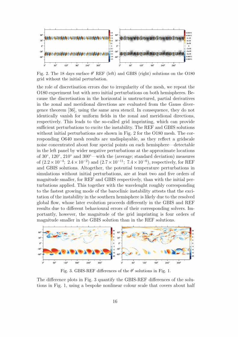
Fig. 2. The 18 days surface θ′ REF (left) and GBIS (right) solutions on the O180grid without the initial perturbation.

the role of discretisation errors due to irregularity of the mesh, we repeat theO180 experiment but with zero initial perturbations on both hemispheres. Be-cause the discretisation in the horizontal is unstructured, partial derivativesin the zonal and meridional directions are evaluated from the Gauss diver-gence theorem [36], using the same area stencil. In consequence, they do notidentically vanish for uniform fields in the zonal and meridional directions,respectively. This leads to the so-called grid imprinting, which can providesufficient perturbations to excite the instability. The REF and GBIS solutionswithout initial perturbations are shown in Fig. 2 for the O180 mesh. The cor-responding O640 mesh results are undisplayable, as they reflect a gridscalenoise concentrated about four special points on each hemisphere—detectablein the left panel by wider negative perturbations at the approximate locationsof 30, 120, 210 and 300—with the (average; standard deviation) measuresof (2.2×10−4; 2.4×10−2) and (2.7×10−11; 7.4×10−6), respectively, for REFand GBIS solutions. Altogether, the potential temperature perturbations insimulations without initial perturbations, are at least two and five orders ofmagnitude smaller, for REF and GBIS respectively, than with the initial per-turbations applied. This together with the wavelenght roughly correspondingto the fastest growing mode of the baroclinic instability attests that the exci-tation of the instability in the southern hemisphere is likely due to the resolvedglobal flow, whose later evolution proceeds differently in the GBIS and REFresults due to different behavioural errors of their corresponding solvers. Im-portantly, however, the magnitude of the grid imprinting is four orders ofmagnitude smaller in the GBIS solution than in the REF solutions.

Fig. 3. GBIS-REF differences of the θ′ solutions in Fig. 1.

The difference plots in Fig. 3 quantify the GBIS-REF differences of the solu-tions in Fig. 1, using a bespoke nonlinear colour scale that covers about half

16

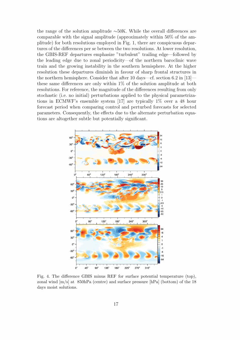
the range of the solution amplitude ∼50K. While the overall differences arecomparable with the signal amplitude (approximately within 50% of the am-plitude) for both resolutions employed in Fig. 1, there are conspicuous depar-tures of the differences per se between the two resolutions. At lower resolution,the GBIS-REF departures emphasize ”turbulent” trailing edge—followed bythe leading edge due to zonal periodicity—of the northern baroclinic wavetrain and the growing instability in the southern hemisphere. At the higherresolution these departures diminish in favour of sharp frontal structures inthe northern hemisphere. Consider that after 10 days—cf. section 6.2 in [13]—these same differences are only within 1% of the solution amplitude at bothresolutions. For reference, the magnitude of the differences resulting from onlystochastic (i.e. no initial) perturbations applied to the physical parametriza-tions in ECMWF’s ensemble system [17] are typically 1% over a 48 hourforecast period when comparing control and perturbed forecasts for selectedparameters. Consequently, the effects due to the alternate perturbation equa-tions are altogether subtle but potentially significant.

Fig. 4. The difference GBIS minus REF for surface potential temperature (top),zonal wind [m/s] at 850hPa (centre) and surface pressure [hPa] (bottom) of the 18days moist solutions.

17

Adding moisture to the problem [41] invigorates the evolution of the barocliniceddies and increases the solution uncertainty [47,12]. 4 This is evidenced inFig. 4 that show the GBIS-REF differences for 18 days moist solutions cor-responding to that shown in the left column of Fig. 3, supplied with plots ofzonal wind at 850hPa and surface pressure. The differences between the moistGBIS and REF results are more apparent. In the northern hemisphere theyare primarily correlated with the steep fronts of the overturning eddies (viz.advanced nonlinearity). In the southern hemisphere, the persistently more ad-vanced development of the instability in the REF solution is still evident.Because moisture substantially complicates gravity wave dynamics [5,1] andenergises spectra in small scales [16], susceptible to truncation and round-offerrors, the consistency of the moist results with the dry solutions indicatesthe dominant role of planetary-scale modulation in retarding the southernhemispheric evolution in the GBIS result. The zonal wind at 850hPa and sur-face pressure are are both weather evolution relevant parameters and clearlyindicate planetary-scale differences.

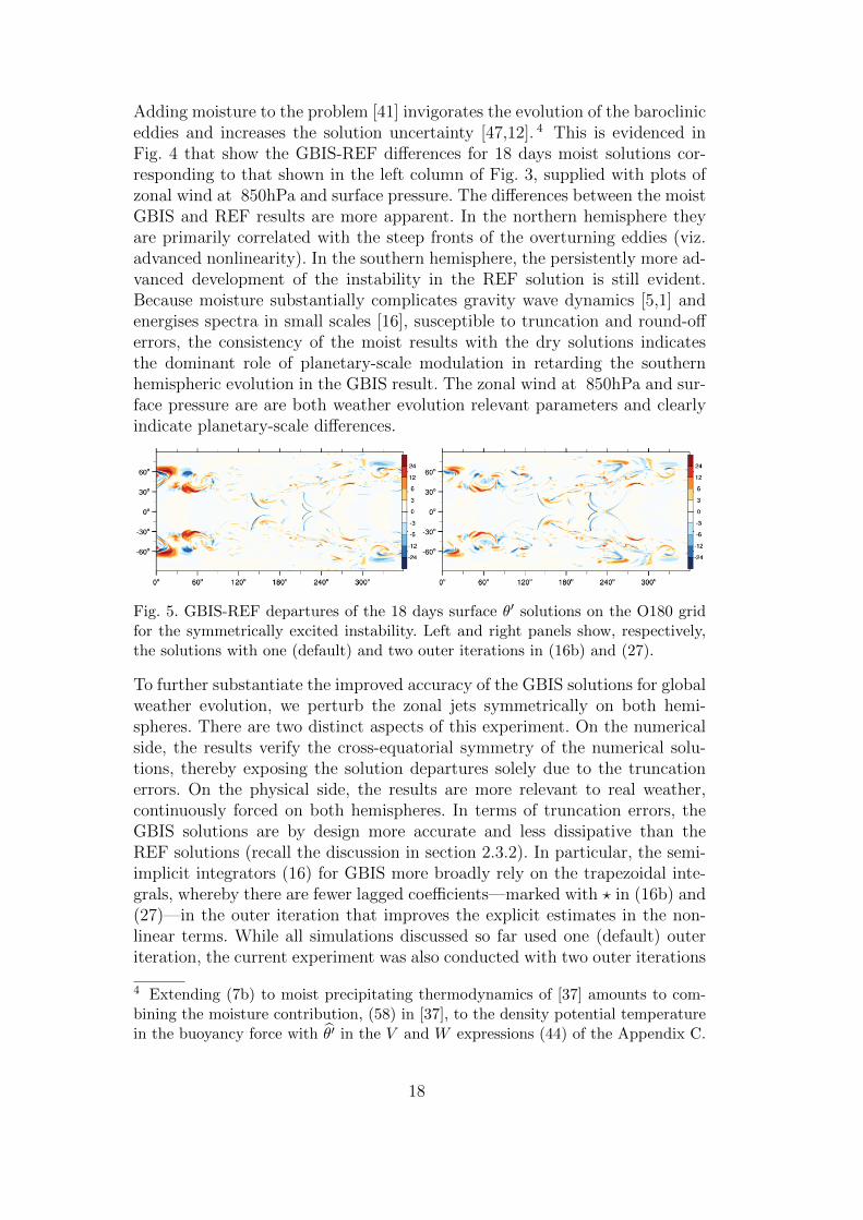
Fig. 5. GBIS-REF departures of the 18 days surface θ′ solutions on the O180 gridfor the symmetrically excited instability. Left and right panels show, respectively,the solutions with one (default) and two outer iterations in (16b) and (27).

To further substantiate the improved accuracy of the GBIS solutions for globalweather evolution, we perturb the zonal jets symmetrically on both hemi-spheres. There are two distinct aspects of this experiment. On the numericalside, the results verify the cross-equatorial symmetry of the numerical solu-tions, thereby exposing the solution departures solely due to the truncationerrors. On the physical side, the results are more relevant to real weather,continuously forced on both hemispheres. In terms of truncation errors, theGBIS solutions are by design more accurate and less dissipative than theREF solutions (recall the discussion in section 2.3.2). In particular, the semi-implicit integrators (16) for GBIS more broadly rely on the trapezoidal inte-grals, whereby there are fewer lagged coefficients—marked with ? in (16b) and(27)—in the outer iteration that improves the explicit estimates in the non-linear terms. While all simulations discussed so far used one (default) outeriteration, the current experiment was also conducted with two outer iterations

4 Extending (7b) to moist precipitating thermodynamics of [37] amounts to com-bining the moisture contribution, (58) in [37], to the density potential temperaturein the buoyancy force with θ′ in the V and W expressions (44) of the Appendix C.

18

in REF and GBIS semi-implicit integrators. Figure 5 shows the hemisphericpatterns of the 18 day GBIS-REF departures of θ′ solutions on the O180 gridwith left and right panels corresponding to the default and two outer iter-ations. Both results evince perfect equatorial symmetry with the GBIS andREF results differing pattern-wise in fine details everywhere but in the re-gion where the wavetrain leading and trailing edges collapse evincing solutiondepartures comparable to the solution amplitude at ∼50%. Moreover, the so-lutions departures are visibly smaller for the runs with two outer iterations.Although this this illustrates the iteration convergence, it does not resolvewhich solver is more accurate. On the other hand, Fig. 6 quantifies the im-pact of the additional iteration on each solver, by showing differences of REF(left) and GBIS (right) results with two and one outer iterations. Clearly theadditional iteration has visibly smaller impact on the GBIS result, which doc-uments that it is REF that approaches GBIS in Fig. 5, and not vice versa.Incidentally, the latter makes the GBIS run effectively cheaper than REF forshort and medium-range applications, because adding the outer iteration toREF with effectively similar solution errors increases its execution time (oth-erwise comparable in both cases) by ∼10%.

Fig. 6. The respective departures of REF (left) and GBIS (right) solutions with twoand one (default) outer iterations.

5 CONCLUDING REMARKS

The key achievement of the technical development summarised in this paper isa novel numerical approach and implementation of perturbation equations formore accurate simulations of all scale atmospheric dynamics. The new pertur-bation form (7) of the compressible Euler equations and the associated numer-ical solvers extend the equivalent apparatus advanced in [35,15,16,36,37] forthe equations formulated in terms of the pressure and entropy perturbationsonto the velocity perturbations. This opens new opportunities for extended-range and seasonal weather and climate applications, by enabling exploitationas well as a dissection of the solution sensitivities to various processes andrealisations of numerical errors.

Apart from the practical consequences of reducing grid imprinting on more

19

flexible but non-uniform meshes, the new formulation requires a learning effortin real applications in order to be used beneficially. The perturbation equationsare formulated about a principally arbitrary ambient state that satisfies thegeneric equations (from which the perturbation forms derive) or a subset. Notall the ambient states are expected to be useful, and a separate research effortis required to identify suitable ambient states for weather simulations with fullcomplexity. The examples provided in this paper assumed a class of idealisedzonally uniform ambient states in a geostrophic balance (31). Such simplestates already expose the complexity of the development, mainly concentratedin the coefficients of the elliptic BVP (27) at the heart of the large-time-stepsemi-implicit integrators (16) for the all-scale compressible Euler equations.

The tailored derivations of the BVP coefficients summarised in Appendices Band C are instructional, as they shed light on the physical significance of thenew development and the associated interpretation of the governing equations.For instance, (39) reveals how the ambient shears modify the Coriolis force,hinting that the trapezoidal integrals of the −v′ · ∇ua terms on the rhs ofthe momentum (vector) equation (7b) should benefit long-term simulations oflarge scale flows dominated by vorticity dynamics. In the established formu-lation (11) the same terms are included in the advection, thus being subjectto truncation terms that serve monotonicity of the transport but dilute theamplitude of the ambient balance, which is circumvented in (7b).

Extended-range simulations of the planetary baroclinic instability illustratethe impact of the new perturbation formulation. As all considered formu-lations are mathematically equivalent, and their associated solvers are for-mally second-order-accurate, we verified no significant differences in short-and medium-range weather evolution. The simulations show that extreme so-lution differences between different formulations are within 1% and 10% ofthe solution amplitude, respectively, after 10 and 15 days of the instabilityevolution, but become comparable to the amplitude (50%) three days later.At this later time there is a marked signal that (7b) offers improved accuracyin the long planetary waves, attributable to a better conditioning of the BVPproblem. Because the accurate representation of the large scales is a prerequi-site for extended-range predictability, the generalised perturbation equationsoffer significant potential for further evaluation.

The hypothesis that GBIS is also more accurate than REF due to an improvedaccuracy of the implicit-shear solutions in planetary scales is corroboratedwith similar EULAG simulations that integrate (11) on a regular longitude-latitude grid, using two variants of the operator preconditioning in the ellipticsolver. The standard deflation preconditioner, common to EULAG and FVM,relies on the direct inversion in the vertical, whereas its optional (in EULAG)ADI extension [21] directly inverts the operator also in the zonal direction.Calculations with the ADI variant evince substantially smaller residual errors

20

on planetary scales (not shown).

All considerations so far exploited a pristine approach with perturbations de-fined with respect to the actual solutions of the generic equations. However,the developed numerical apparatus offers technical advantages equally ap-plicable to approximate ambient states constructed based on alternative orsurrogate models and/or (machine-learned) data. This may call for the inclu-sion of additional forcing terms (bias correction) to model the ambient stateerrors as opposed to bias correcting the entire state evolution —in the spiritof turbulence closures or continuous data assimilation [3]. However, impor-tantly this will not affect the machinery of the semi-implicit integrators andthe BVP coefficients. Consequently, the proposed solvers form the basis for thedevelopment of new multilevel methods, time parallel and/or hardware-failureresilient algorithms as well as blending with novel data-informed approaches.

Acknowledgements: This work was supported in part by funding received fromthe European Research Council under the European Union’s Seventh Frame-work Programme (FP7/2012/ERC Grant agreement no. 320375).

Appendix A. Specifications of the spherical frame

In the spherical curvilinear framework of [22], the vector u represents thephysical velocity with components aligned at every point of the spherical shellwith axes of a local Cartesian frame (subsequently marked as c) tangent to thelower surface (r = a) of the shell; r is the radial component of the vector radius,and a is the radius of the sphere, cf. Fig. 7.7, section 7.2 in [7]. Consequently,dxc = r cosφ dλ, dyc = r dφ and zc = r−a; where λ and φ denote longitude andlatitude angles, respectively. Then, in the formalism of Sections 2 and 3 andin the absence of coordinate stretching, x = aλ, y = aφ, and z = zc; therebyeffectively employing longitude-latitude coordinates standard in many globalatmospheric models [38]. Furthermore, the coefficient matrix G consists of zerooff-diagonal entries, whereas G1

1 = [Γ cos(y/a)]−1, G22 = Γ−1, and G3

3 = 1. Here,Γ = 1 + χ z/a, and indices 1, 2, and 3 correspond to x, y, and z components.Consequently, the Jacobian is G = Γ2 cos(y/a). The parameter χ is set to unityby default; whereas the optional setting χ = 0 selects the shallow atmosphereapproximation in the governing PDEs [44].

In the momentum equation, the components of the Coriolis acceleration are

21

−f × u =[v f0 sin(y/a)− χw f0 cos(y/a) , (32)

−u f0 sin(y/a) ,

χ u f0 cos(y/a)],

where u = [u, v, w] and f0 = 2|Ω|. Furthermore, the metric forcings (viz.,component-wise Christoffel terms associated with the convective derivative ofthe physical velocity) are,

MMM(u) = (Γa)−1[

tan(y/a)u v − χ uw , (33)

− tan(y/a)uu− χ v w ,

χ (uu+ v v)].

Appendix B. Details of the linear operator on the lhs of(23a)

Expanding (21) in components leads to

u′x+τu

(u′x∂xu

xa + u′

y∂yu

xa + u′

z∂zu

xa

)+ τu

(−u′ yf z + u′

zf y)

−τuτ θ(u′x∂xΘa + u′

y∂yΘa + u′

z∂zΘa

)∂xφa =

u′ x − τuΘ?∂xφ

′ ,(34a)

u′y+τu

(u′x∂xu

ya + u′

y∂yu

ya + u′

z∂zu

ya

)+ τu

(−u′ zfx + u′

xf z)

−τuτ θ(u′x∂xΘa + u′

y∂yΘa + u′

z∂zΘa

)∂yφa =

u′ y − τu Θ?∂yφ

′ ,(34b)

u′z+τu

(u′x∂xu

za + u′

y∂yu

za + u′

z∂zu

za

)+ τu

(−u′ xf y + u′

yfx)

−τuτ θ(u′x∂xΘa + u′

y∂yΘa + u′

z∂zΘa

)∂zφa =

u′ z − τu Θ?∂zφ

′ ,(34c)

which upon regrouping all terms in the spirit of a matrix-vector product,

u′x[1+τu(∂xu

xa − τ θ∂xΘa∂xφa)]

+u′y[τu(∂yu

xa − τ θ∂yΘa∂xφa − f z)]

+u′z[τu(∂zu

xa − τ θ∂zΘa∂xφa + f y)] =

u′ x − τu Θ?∂xφ

′ ,

(35a)

u′x[τu(∂xu

ya − τ θ∂xΘa∂yφa + f z)]

+u′y[1+τu(∂yu

ya − τ θ∂yΘa∂yφa)]

+u′z[τu(∂zu

ya − τ θ∂zΘa∂yφa − fx)] =

u′ y − τu Θ?∂yφ

′ ,

(35b)

u′x[τu(∂xu

za − τ θ∂xΘa∂zφa − f y)]

+u′y[τu(∂yu

za − τ θ∂yΘa∂zφa + fx)]

+u′z[1+τu(∂zu

za − τ θ∂zΘa∂zφa)] =

u′ z − τu Θ?∂zφ

′ ,

(35c)

22

reveals the entries of the linear operator L = [lij] in (23a) as

l11 = 1 + τu(∂xuxa − τ θ∂xΘa∂xφa) ,

l12 = τu(∂yuxa − τ θ∂yΘa∂xφa − f z) ,

l13 = τu(∂zuxa − τ θ∂zΘa∂xφa + f y) ,

(36a)

l21 = τu(∂xuya − τ θ∂xΘa∂yφa + f z) ,

l22 = 1 + τu(∂yuya − τ θ∂yΘa∂yφa) ,

l23 = τu(∂zuya − τ θ∂zΘa∂yφa − fx) ,

(36b)

l31 = τu(∂xuza − τ θ∂xΘa∂zφa − f y) ,

l32 = τu(∂yuza − τ θ∂yΘa∂zφa) + fx) ,

l33 = 1 + τu(∂zuza − τ θ∂zΘa∂zφa) .

(36c)

Having defined all entries of L, its inverse is evaluated as analytically as L−1 =L−1adj(L) where L ≡ det(L) and “adj” denotes the matrix adjugate, withcolumn-wise entries:

adjl11 = l22l33 − l23l32 ,adjl21 = l23l31 − l21l33 ,adjl31 = l21l33 − l23l31 ,

(37a)

adjl12 = l13l32 − l12l33 ,adjl22 = l11l33 − l13l31 ,adjl32 = l12l31 − l11l32 ,

(37b)

adjl13 = l12l23 − l13l22 ,adjl23 = l13l21 − l11l23 ,adjl33 = l11l22 − l12l21 .

(37c)

Appendix C. Further details of the Poisson problem (28)

To highlight the connection of the matrix-algebra formalism of Appendix Bwith hand-derived compact formulae of [22], it is instructive to specify furtherdetails of (28), for the perturbation equations (7) and a class of zonally-uniformambient states (31) assumed in Sections 3.2.2 and 4. In particular, when solv-ing (7b), accounting for ϑx ≡ 0 and adopting normalisations accordant with[22] (to be explained shortly),

E −1 = [G3F2F3 + G2(1+F2F2)]ϑy + [G2F2F3 + G3(1 + F3F3)]ϑz

+(1+α∗)(1 + F2F2 + F3F3) .(38)

23

Here G2 and G3 correspond to normalised meridional and radial componentsof θ−10 G∇φa, and

F2 = F2 + ∂∗zua , F3 = F3 − ∂∗yua, (39)

where the symbols Fj, ϑζ , α∗ correspond to normalised components of the

Coriolis parameter, components of the ambient gradients ∇Θa and αθ, andthe asterisk by ∂y, ∂z marks the normalisation.

The functions V p and C pk from the rhs of (29) are compactly written as

V 1 = A U + BV −X W ,

V 2 = CU + DV + Y W ,

V 3 = H U + I V + ZW .

(40)

where the coefficients A to I (named after [22]) and X to Z (introducedhere for conciseness) are equal to

A = R + G2ϑy + G3ϑz ,

B = RF3 + G3(F2ϑy + F3ϑz) ,

X = −RF2 − G2(F2ϑy + F3ϑz) ,

(41)

C = −RF3 − (G2F2 + G3F3)ϑz ,

D = R(1 + F2F2) + G3ϑz ,

Y = RF2F3 − G2ϑz ,

(42)

and

H = RF2 + (G2F2 + G3F3)ϑy ,

I = RF2F3 − G3ϑy ,

Z = R(1 + F3F3) + G2ϑy

(43)

Here as well as in (38) and the model code, R = τu/τ θ (recall Eqs. 19),whereas all the components of the Coriolis parameter, ambient gradients ∇Θa

and generalised buoyancy θ−10 G∇φa are multiplied by τu, in effect of which thefactor (1 + α∗)−1 ≡ τuδ−1h t in the corresponding formulae of [22] is absorbedin definitions of the normalised fields. Furthermore, the velocities U , V andW are

U =β u+ ua ,

V =β v + G2θ′ + δhtf3ua ,

W =β w + G3θ′ − δhtf2ua ,(44)

where β = δht/τu is the reciprocal of the normalising prefactor in (22), 5 and

Gk = Gk/R.

5 Note two typos in (A.16) of [22]: θ′ should be LE(θ′) and θ′ = θ − θe, for consis-

24

The coefficients C pk used in (29) take the explicit form:

C 11 =R(G11 + G1

2F3) + G2G11ϑy + G3

[G1

2F2ϑy + (G11 + G1

2F3)ϑz],

C 12 =R(G21 + G2

2F3) + G2G21ϑy + G3

[G2

2F2ϑy + (G21 + G2

2F3)ϑz],

C 13 =R(G31 + G3

2F3 − G33F2) + G3

[G3

2F2ϑy + (G31 + G3

2F3)ϑz]

+ Gy[−G3

3F3ϑz + (G31 − G3

3F2)ϑy],

(45)

C 21 =R[−G1

1F3 + G12(1 + F2F2)

]−[G2G

11F2 − G3(G

12 − G1

1F3)]ϑz ,

C 22 =R[−G2

1F3 + G22(1 + F2F2)

]−[G2G

21F2 − G3(G

22 − G2

1F3)]ϑz ,

C 23 =R[−G3

1F3 + G32(1 + F2F2) + G3

3F2F3

]+[G3(G

32 − G3

1F3)− G2(G33 + G3

1F2)]ϑz ,

(46)

C 31 =R(G11F2 + G1

2F2F3) +[G2G

11F2 + G3(G

11F3 − G1

2)]ϑy ,

C 32 =R(G21F2 + G2

2F2F3) +[G2G

21F2 + G3(G

21F3 − G2

2)]ϑy ,

C 33 =R[G3

1F2 + G32F2F3 + G3

3(1 + F3F3)]

+[G2(G

31F2 + G3

3) + G3(G31F3 − G3

2)ϑy].

(47)

The provided expressions are general, in that they account for all the fourforms of the considered perturbation equations. Namely, for (10)

G2 ≡ 0, G3 ≡ G , (48)

where G is the normalised gravitational acceleration of [22]; whereas for (12)

F2 ≡ F2 , F3 ≡ F3 . (49)

Furthermore, (11) combines (48) and (49), reproducing the formulae of [22]—all under the assumption of ϑx ≡ 0. Consequently, the compact modifications(48) and (49) verify the field E specified in (A.4) of [22], the explicit V p = ˇup/Evelocities in their formulae (A.5)-(A.7) as well as the coefficients A -I intheir (A.8)-(A.15). The latter coefficients correspond to the entries of theL−1E −1 operator that (here) acts on the explicit counterpart of the physical

velocityu′ + Lua—the components of which correspond in turn to U , V and

W converted to V p|p=1,2,3 in (A.5)-(A.7) of [22] and specified in their (A.14)-(A.16). Furthermore, these modifications also verify the C pk coefficients in(A.17)-(A.25).

tency with their Eq. (12).

25

References

[1] I. Barstad, W.W. Grabowski, P.K. Smolarkiewicz, Characteristics of large-scaleorographic precipitation: Evaluation of linear model in idealized problems, J.Hydrol. 340 (2007) 78-90.

[2] P. Bauer, A. Thorpe, G. Brunet, The quiet revolution of numerical weatherprediction, Nature 525 (2015) 47–55.

[3] J.-F. Cossette, P. Charbonneau, P.K. Smolarkiewicz, M.P. Rast, Magnetically-modulated heat transport in a global simulation of solar magneto-convection,Astrophysics. J. 841 (2017) 65 (17pp).

[4] A. Dornbrack, J.D. Doyle, T.P. Lane, R.D. Sharman, P.K. Smolarkiewicz, Onphysical realizability and uncertainty of numerical solutions, Atmos. Sci. Let. 6(2005) 118-122. doi:10.1002/asl.100

[5] D.R. Durran, J.B. Klemp, A compressible model for the simulation of moistmountain waves, Mon. Weather Rev. 111 (1983) 2341–2361.

[6] D.R. Durran, Improving the anelastic approximation. J. Atmos. Sci. 46 (1989)1453–1461.

[7] J.A. Dutton, The Ceaseless Wind, Dover Publications (1986) pp. 617.

[8] M. Ghizaru, P. Charbonneau, P.K. Smolarkiewicz, Magnetic Cycles in GlobalLarge-eddy Simulations of Solar Convection, Astrophys. J. Lett. 715 (2010)L133–L137

[9] https://hiwpp.noaa.gov/.

[10] C. Jablonowski, D.L. Williamson, A baroclinic instability test case foratmospheric model dynamical cores, Q.J.R. Meteorol. Soc. 132 (2006) 2943–2975.

[11] C. Kuhnlein, P.K. Smolarkiewicz, A. Dornbrack, Modelling atmospheric flowswith adaptive moving meshes, J. Comput. Phys. 231 (2012) 2741–2763.

[12] C. Kuhnlein, C. Keil, G.C. Craig, C. Gebhardt, The impact of downscaled initialcondition perturbations on convective-scale ensemble forecasts of precipitation,Q. J. Roy. Meteorol. Soc., 140 (2014) 1552–1562.

[13] C. Kuhnlein, P.K. Smolarkiewicz, An unstructured-mesh finite-volumeMPDATA for compressible atmospheric dynamics, J. Comput. Phys. 334 (2017),16–30.

[14] C. Kuhnlein, S. Malardel, P.K. Smolarkiewicz, Simulation in the greyzone withthe Finite-Volume Module of the IFS, Workshop: Shedding light on the greyzone,ECMWF, Reading, 13-16 Nov. 2017; https://www.ecmwf.int/sites/default/files/elibrary/2017/17804-simulation-greyzone-finite-volume-module-ifs.pdf

26

[15] M.J. Kurowski, W.W. Grabowski, and P.K. Smolarkiewicz, Anelastic andcompressible simulations of moist deep convection, J. Atmos. Sci. 71 (2014) 3767–3787.

[16] M.J. Kurowski, W.W. Grabowski, and P.K. Smolarkiewicz, Anelastic andcompressible simulations of moist dynamics at planetary scales, J. Atmos. Sci.72 (2015) 3975–3995.

[17] M. Leutbecher et al., Stochastic representations of model uncertainties atECMWF: state of the art and future vision, Q.J. Roy. Meteorol. Soc., 143 (2017)2315–2339.

[18] F.B. Lipps, R.S. Hemler, A scale analysis of deep moist convection and somerelated numerical calculations, J. Atmos. Sci. 39 (1982) 2192–2210.

[19] H.R., Miller, 1991: A horror story about integration methods, J. Comput. Phys.,93 (1991) 469–476.

[20] L. Magnusson, M. Alonso-Balmaseda, S. Corti, F. Molteni, T. Stockdale,Evaluation of forecast strategies for seasonal and decadal forecasts in presenceof systematic model errors, Clim. Dyn. (2013), 41:23932409.

[21] Z.P. Piotrowski, B. Matejczyk, L. Marcinkowski, P.K. Smolarkiewicz, ParallelADI preconditioners for all-scale atmospheric models, in Parallel Processing andApplied Mathematics, LNCS 9574, Springer International Publishing, 607-618.

[22] J.M. Prusa, P.K. Smolarkiewicz, An all-scale anelastic model for geophysicalflows: dynamic grid deformation, J. Comput. Phys. 190 (2003) 601–622.

[23] J.M. Prusa, P.K. Smolarkiewicz, A.A Wyszogrodzki, EULAG, a computationalmodel for multiscale flows, Comput. Fluids 37 (2008) 1193–1207

[24] E. Racine, P. Charbonneau, M. Ghizaru, A. Bouchat, P.K. Smolarkiewicz, Onthe mode of dynamo action in a global large-eddy simulation of solar convection,Astrophys. J. 735:46 (2011) 22 pp.

[25] P.K. Smolarkiewicz, L.G. Margolin, Variational solver for elliptic problems inatmospheric flows, Appl. Math. Comp. Sci. 4 (1994) 527–551.

[26] P.K. Smolarkiewicz, L.G. Margolin, A.A Wyszogrodzki, A class ofnonhydrostatic global models, J. Atmos. Sci. 58 (2001) 349–364.

[27] P.K. Smolarkiewicz, L.G. Margolin: On forward-in-time differencing for fluids:an Eulerian/semi-Lagrangian non-hydrostatic model for stratified flows, Atmos.-Ocean, 35 (1997) 127–152.

[28] P.K. Smolarkiewicz, J.A. Prusa, Towards mesh adaptivity for geophysicalturbulence: continuous mapping approach, Int. J. Numer. Meth. Fluids 47 (2005)789–801.

[29] P.K. Smolarkiewicz, J. Szmelter, MPDATA: An edge-based unstructured-gridformulation, J. Comput. Phys. 206 (2005) 624-649.

27

[30] P.K. Smolarkiewicz, Multidimensional positive definite advection transportalgorithm: an overview, Int. J. Numer. Meth. Fluids 50 (2006) 1123–1144.

[31] P.K. Smolarkiewicz, R. Sharman, J. Weil, S.G. Perry, D. Heist, G. Bowker,Building resolving large-eddy simulations and comparison with wind tunnelexperiments, J. Comput. Phys. 227 (2007) 633–653.

[32] P.K. Smolarkiewicz, A. Dornbrack, Conservative integrals of adiabaticDurran’s equations, Int. J. Numer. Meth. Fluids 56 (2008) 1513–1519.doi: 10.1002/fld.1601

[33] P.K. Smolarkiewicz, J. Szmelter, A nonhydrostatic unstructured-meshsoundproof model for simulation of internal gravity waves, Acta Geophysica 59(2011) 1109–1134.

[34] P.K. Smolarkiewicz, P. Charbonneau, EULAG, a computational model formultiscale flows: An MHD extension, J. Comput. Phys. 236 (2013) 608–623.

[35] P.K. Smolarkiewicz, C. Kuhnlein, N.P. Wedi, A consistent framework fordiscrete integrations of soundproof and compressible PDEs of atmosphericdynamics, J. Comput. Phys. 263 (2014) 185-205

[36] P.K. Smolarkiewicz, W. Deconinck, M. Hamrud, C. Kuhnlein, G. Mozdzynski,J. Szmelter, N.P. Wedi, A finite-volume module for simulating global all-scaleatmospheric flows, J. Comput. Phys. 315 (2016) 287–304.

[37] P.K. Smolarkiewicz, C. Kuhnlein, W.W. Grabowski, A finite-volume modulefor cloud-resolving simulations global atmospheric flows, J. Comput. Phys. 341(2017) 208–229.

[38] J. Szmelter, P.K. Smolarkiewicz, An edge-based unstructured meshdiscretisation in geospherical framework, J. Comput. Phys. 229 (2010) 4980–4995.

[39] A. Warn-Varnas, J. Hawkins, P.K. Smolarkiewicz, S.A. Chin-Bing, D. King, Z.Hallock, Solitary wave effects north of Strait of Messina, Ocean Modelling 18(2007) 97–121.

[40] P.A. Ullrich, T. Melvin, C. Jablonowski, A. Staniforth, A proposed baroclinicwave test case for deep- and shallow-atmosphere dynamical cores, Q.J. Roy.Meteorol. Soc., 140 (2014) 1590–1602.

[41] P.A. Ullrich, C. Jablonowski, K.A. Reed, C. Zarzycki, P.H. Lauritzen, R.D.Nair, J. Kent, A. Verlet-Banide, Dynamical core model intercomparison project(DCMIP2016) test case document,https://github.com/ClimateGlobalChange/DCMIP2016.

[42] N.P. Wedi, P.K. Smolarkiewicz, Extending Gal-Chen and Somerville terrain-following coordinate transformation on time dependent curvilinear boundaries,J. Comput. Phys. 193 (2004) 1–20.

[43] N.P. Wedi, P.K. Smolarkiewicz, Direct numerical simulation of the Plumb-McEwan laboratory analog of the QBO, J. Atmos. Sci. 63 (2006) 3326–3252.

28

[44] N.P. Wedi, P.K. Smolarkiewicz, A framework for testing global nonhydrostaticmodels, Q.J. Roy. Meteorol. Soc., 135 (2009) 469–484.

[45] N.P. Wedi, P.K. Smolarkiewicz, A nonlinear perspective on the dynamics of theMJO: idealized large-eddy-simulations, J. Atmos. Sci. 67 (2010) 1202–1217.

[46] N.P. Wedi, P. Bauer, W. Deconinck, M. Diamantakis, M. Hamrud, C. Kuhnlein,S. Malardel, K. Mogensen, G. Mozdzynski, P.K. Smolarkiewicz, The modellinginfrastructure of the Integrated Forecasting System: Recent advances and futurechallenges, Technical Memorandum 760 (2015), ECMWF, pp. 48.

[47] F. Zhang, N. Bei, R. Rotunno, C. Snyder, Mesoscale predictability of moistbaroclinic waves: convection-permitting experiments and multistage error growthdynamics, J. Atmos. Sci. 64 (2007) 3579–3594.

29