
Personal Exposure to Contaminant Sources in Ventilated Rooms
266
Personal Exposure to Contaminant Sources in Ventilated Rooms by Henrik Brohus This thesis is accepted for the degree of Doctor of Philosophy at the Faculty of Engineering and Science, Aalborg University, Denmark. Defended publicly at Aalborg University April 24, 1997. Supervisor: Peter V. Nielsen, Professor, Aalborg University, Denmark Adjudication Committee: P.O. Fanger, Professor, Technical University of Denmark, Denmark Lars Olander, Professor, National Institute of Working Life, Sweden Per Heiselberg, Associate Professor, Aalborg University, Denmark ISSN 0902-7953 R9741
Transcript of Personal Exposure to Contaminant Sources in Ventilated Rooms

Personal Exposure to ContaminantSources in Ventilated Rooms
by
Henrik Brohus
This thesis is accepted for the degree of Doctor of Philosophy at the Faculty ofEngineering and Science, Aalborg University, Denmark. Defended publicly atAalborg University April 24, 1997.
Supervisor:Peter V. Nielsen, Professor, Aalborg University, Denmark
Adjudication Committee:P.O. Fanger, Professor, Technical University of Denmark, DenmarkLars Olander, Professor, National Institute of Working Life, SwedenPer Heiselberg, Associate Professor, Aalborg University, Denmark
ISSN 0902-7953 R9741

Henrik BrohusPersonal Exposure to Contaminant Sources in Ventilated RoomsPh.D.-ThesisISSN 0902-7953 R9741Printed by Kolding Trykcenter, Denmark
Aalborg UniversityDepartment of Building Technology and Structural EngineeringSohngaardsholmsvej 57DK-9000 AalborgDenmark
Phone: +45 9635 8539Fax: +45 9814 8243E-mail: [email protected]: www.civil.auc/i6/klima

Preface 1
Preface
This thesis is submitted in accordance with the conditions for attaining the DanishPh.D.-degree.
It represents the end of my Ph.D.-study at Aalborg University, Department ofBuilding Technology and Structural Engineering with Prof. Peter V. Nielsen assupervisor.
This research was supported financially by the Danish Technical ResearchCouncil (STVF) as part of the research programme “Healthy Buildings”, 1993 -1997.
I wish to express my gratitude to Prof. Peter V. Nielsen for his guidance and forgiving me the opportunity to fulfil this work.
My thanks also extend to Prof. P. Ole Fanger, Dr. Geo Clausen, Dr. HenrikKnudsen, Dr. Jan Pejtersen and the rest of the staff at the Laboratory of Heatingand Air Conditioning for their hospitality and support during my stay at theTechnical University of Denmark.
I would like to thank colleagues and members of the technical staff for theirvaluable assistance during the study. Especially, I want to thank TorbenChristensen and Carl Erik Hyldgård for assistance in the laboratory, Bente JulKjærgaard for linguistic support, Norma Hornung for the drawings, and Dr. KjeldSvidt for passing remarks on the work.
Finally, I want to thank my beloved family for their patience and support.
Henrik Brohus
February 1997

Henrik Brohus2

Abstract 3
Abstract
Exposure models usually treat the indoor environment as well-mixedcompartments without concentration gradients. However, in practiceconcentration gradients will occur, for instance, in the vicinity of contaminantsources or in the case of displacement ventilation.
When a person is located in a room where concentration gradients prevail, thelocal concentration distribution may be changed significantly and thus thepersonal exposure.
Three different tools for personal exposure assessment are presented. They are allable to consider the local influence of persons in ventilated rooms whereconcentration gradients prevail:
- the Breathing Thermal Manikin- the Computer Simulated Person- the Trained Sensory Panel
The tools are applied on the two major room ventilation principles, namely thedisplacement principle and the mixing principle. This is done in order to examinethe tools and to investigate how the exposure assessment is influenced whenconcentration gradients and persons are considered.
A personal exposure model for a displacement ventilated room is proposed.
Two new quantities describing the interaction between a person and theventilation are defined.
The findings clearly stress the need for an improved exposure assessment in caseswhere a contaminant source is located in the vicinity of persons.
It is also shown that it is not sufficient to know the local concentration level of anempty room, the local impact of a person is distinct and should be considered inthe exposure assessment.

Henrik Brohus4

Contents 5
Contents
Preface 1
Abstract 3
Contents 5
Chapter 1. Introduction 9
1.1. Importance of the indoor climate 91.2. Personal exposure assessment 101.3. Definitions 121.4. Aims and scope 15
Chapter 2. Tools for personal exposure assessments 17
2.1. Introduction 172.2. Breathing Thermal Manikin 18
2.2.1. Introduction 18
2.2.2. Heat transfer from persons 18
2.2.2.1. Modes of heat transfer 182.2.2.2. Convection 222.2.2.3. Radiation 32
2.2.3. Respiration 35
2.2.4. Description of the Breathing Thermal Manikin 38
2.2.4.1. Introduction 382.2.4.2. Construction of manikin 39

Henrik Brohus6
2.2.5. Personal exposure assessment using the BTM 42
2.3. Computer Simulated Person 43
2.3.1. Introduction 43
2.3.2. Computational Fluid Dynamics 44
2.3.2.1. Governing equations 442.3.2.2. Numerical solution of equations 512.3.2.3. Boundary conditions 522.3.2.4. Software 57
2.3.3. Description of Computer Simulated Person 58
2.3.3.1. Introduction 582.3.3.2. Geometry and boundary conditions of models 59
2.3.4. Personal exposure assessment using CSP 64
2.4. Trained Sensory Panel 67
2.4.1. Introduction 672.4.2. Assessment of perceived air quality 682.4.3. Personal exposure assessment using the TSP 74
Chapter 3. Displacement ventilation 77
3.1. Introduction 77
3.2. Characteristics of displacement ventilation 78
3.3. Measurements using a BTM 83
3.3.1. Experimental set-up 833.3.2. Exposure in proportion to stratification height 883.3.3. Personal exposure model for a displacement ventilated room 933.3.4. Exposure in proportion to location of a
passive point contaminant source 105

Contents 7
3.4. Measurements using a TSP 114
3.4.1. Experimental set-up 1153.4.2. Perceived air quality in a displacement ventilated room 1193.4.3. Effect of entrainment in the human boundary layer 124
3.5. Simulations using a CSP 128
3.5.1. Geometry and boundary conditions 1283.5.2. Simulation of the flow field 1313.5.3. Simulation of personal exposure 137
3.6. Conclusion 146
Chapter 4. Mixing ventilation 149
4.1. Introduction 149
4.2. Unidirectional flow field 150
4.2.1. Experimental set-up 1514.2.2. Measurements using a BTM 1534.2.3. CFD simulation 1634.2.4. Simulation of personal exposure 1734.2.5. Comparison with exposure models 186
4.3. Mixing ventilated room 194
4.3.1. Geometry and boundary conditions 1944.3.2. Simulation of the flow field 1964.3.3. Simulation of personal exposure 203
4.4. Conclusion 211
Chapter 5. General discussion and conclusion 213
Henrik Brohus8
Appendix A. Heat balance for a person 221
A.1. Steady-state total heat balance for a person 221A.2. Heat loss by respiration 222A.3. Latent heat loss 223A.4. Skin temperature vs. sensible heat loss 224A.5. Surface temperature vs. insulation value of clothing 225
Appendix B. Surface areas of theBreathing Thermal Manikin 227
Appendix C. Measurement of the convectiveheat transfer coefficient 229
C.1. Measurement set-up 229C.2. Radiative heat transfer coefficient 231C.3. Convective heat transfer coefficients 231
Appendix D. Measurement of the clothing insulation 235
D.1. Theory 235D.2. Results 236
Appendix E. k - εεεε Transport equations 239
Appendix F. t-test 241
Sammendrag på dansk 243
References 249
Nomenclature 259
Chapter 1 Introduction 9
Chapter 1
Introduction
1.1. Importance of the indoor climate
In the industrial countries people spend the major part of their time in an indoorenvironment. Many people spend more than 90% of their time in an artificialclimate i.e., offices, factories, public buildings, homes, transport vehicles etc.(Turiel, 1985; Awbi, 1991).
This fact stresses the importance of a healthy and comfortable indoor climate bothregarding thermal comfort, indoor air quality, and other parameters constitutingthe indoor climate perceived by the occupants. In this thesis, the matter inquestion is the air quality.
Indoor air pollution
The indoor air is a complex mixture of outdoor air and different kinds ofpollutants generated in the indoor environment. The outdoor air quality may varyfrom one location to another depending on possible outdoor contaminant sources,e.g. exhaust air from neighbouring buildings ventilation system, discharge fromindustrial processes, traffic etc.
Indoor air pollution (IAP) comes from the outdoor air, building materials,furniture and equipment, man and his activities. IAP may be inorganic pollutants(CO2, CO, SO2, NOx etc.), organic pollutants (volatile organic compounds etc.),particulate matter, fibres, environmental tobacco smoke, radon, and differentbiological agents (house dust mites, fungi, and bacteria etc.). (McCarthy et al.,1991; Maroni et al., 1995).

Henrik Brohus10
Indoor environmental problems
Numerous cases of health complaints among employees in office buildings haveoccurred since the early 1970s. The complaints can be divided into two categories“those characterised by a generally clinical picture for which a specific cause hasbeen identified, and those in which affected workers reported nonspecificsymptoms occurring only during the time they were at work” (ECA, 1991). Thefirst category is defined as the “building-related illness” (BRI) and the secondcategory is defined as the “sick building syndrome” (SBS). Symptoms reported inSBS include mucous membrane and eye irritation, cough, chest tightness, fatigue,headache and malaise (Maroni et al., 1995).
A recent study on the indoor air quality in 56 European office buildings in ninecountries reported that 30% of the occupants perceived the air as unacceptablealthough the average ventilation rate was way above existing national ventilationstandards (Fanger, 1995).
Occupational health problems
While office workers are usually exposed to a larger number of indoor airpollutants at a low concentration, industrial workers may be exposed to fewercontaminants but at a higher concentration level. Serious health problems mayoccur if the workers are not sufficiently protected against exposure to thecontaminants found in the industry.
1.2. Personal exposure assessment
The fact that many people spend the major part of their time in an artificial indoorenvironment, where they are subject to various contaminant sources, emphasisesthe importance of a proper exposure assessment.

Chapter 1 Introduction 11
Concentration gradients in ventilated rooms
When personal exposure in a ventilated room is to be determined one may chooseto perform a series of measurements or to use a model for calculation. Bothapproaches may lead to erroneous results if they are not treated properly.
Exposure models usually treat the indoor microenvironments as well mixedcompartments where the concentration of a certain component is found by asimple mass balance (Maroni et al., 1995). When the ventilated room is addressedthe air is thus regarded as being fully mixed which implies that no concentrationgradients exist.
Rodes et al. (1991) summarise various measurements from the literature and statethat there may be considerable deviations between measurements using personalexposure monitors (PEM) and microenvironmental monitors (MEM). TypicalPEM/MEM ratios were found in the interval from 1.58 to 13.40. In practice concentration gradients will occur, for instance in the vicinity ofcontaminant sources and also in case of displacement ventilation, wherecontaminant stratification with considerable gradients is utilised to improve theventilation effectiveness (Brohus and Nielsen, 1996b).
Interaction between a person and the environment
When a person is located in a ventilated room where concentration gradientsprevail, the local concentration field may be changed significantly and thus thepersonal exposure. The reason is the local change in the flow field caused by thepresence of the person, e.g. due to:
… the excess surface temperature of the human body generates a convectiveascending air current along the body. This convective flow may entrain acontaminant in the lower part of the room and transport it to the breathing zone.In that way a person may be exposed to a concentration deviating substantiallyfrom the general concentration in the breathing zone height in other parts of theroom.
… a person may locally act as an obstacle to the general flow field. For instance,if the person is exposed to a flow field coming from behind a wake is generated in

Henrik Brohus12
front of the person. This wake may entrain contaminant from a distance exceedinghalf a metre.
… when a person is moving the local flow field and the local contaminant fieldmay change significantly. The effect of the ascending air flow in the humanboundary layer will decrease according to the movements. The movements mayalso affect the general flow field and, therefore, indirectly the local field and thusthe personal exposure.
If more persons are located near each other they may also affect the flow fieldand, furthermore, the exhalation from one person may penetrate another person’sbreathing zone and cause exposure (Bjørn and Nielsen, 1995; 1996).
Improved exposure models
The previous discussion raises a need for exposure models which are able toconsider the local effect of persons located in ventilated rooms whereconcentration gradients prevail.
1.3. Definitions
Ventilation effectiveness
To describe the efficiency of an air distribution system, different quantities arecommonly used. The mean ventilation effectiveness, ε , is defined as
ε =c
cR (1.1)
where cR is the concentration in the return opening and c is the meanconcentration in the room. The ventilation effectiveness in the occupied zone, εoc,is given by
εocR
oc
c
c= (1.2)

Chapter 1 Introduction 13
where coc is the mean concentration in the occupied zone. Here, the occupied zoneis defined as the area up to 1.8 m above floor level.
The local ventilation index, εP, is defined as
εPR
P
c
c= (1.3)
where cP is the concentration at a point in the room.
A new ventilation effectiveness will here be defined: the personal exposure index,designated εe
εeR
e
c
c= (1.4)
where ce is the concentration of inhaled contaminant. The personal exposure indexexpresses the effectiveness actually experienced by a person in the ventilatedroom. The new quantity and its use is discussed in more detail below.
Equations (1.1) to (1.4) assume that the supply air is uncontaminated.
Concentration, exposure and dose
Before the topic “personal exposure” is further discussed, it may be convenient toclarify the differences between the concepts of concentration, exposure and dose.
Exposure requires, strictly speaking, the simultaneous occurrence of two events: apollutant concentration at a particular place and time, and the presence of aperson at that place and time (Sexton and Ryan, 1988). Expressed in anotherway, exposure is defined as the event during which a person comes into contactwith a pollutant.
Dose occurs when the pollutant actually crosses the physical boundary of aperson. consequently, there can be an exposure without a dose but there cannot bea dose without an exposure (Ott, 1985). This implies that persons exposed to thesame level may receive different doses if the pulmonary ventilation varies due todifferent activity levels (Tjelflaat, 1992; Brohus and Nielsen, 1994b).

Henrik Brohus14
The concentration of inhaled contaminant, ce, corresponds to the exposure of aperson. It represents the event during which a person is in contact with apollutant. Subsequently ce is designated “exposure” as well as “concentration ofinhaled contaminant”.
To compare the exposure and the concentration, cP, measured at a “neutral” pointat the breathing zone height, both quantities should in theory be determined at thesame location, but in case of cP without the local influence of the person(movements, convective boundary layer flow, etc.). In this way the differencebetween εe and εP is due solely to the person´s presence. The importance ofmaking this distinction will appear clearly in the following chapters.
In practice, cP is measured at the breathing zone height outside the thermalboundary layer some distance away from the person. Alternatively, the person inquestion is temporarily moved while measuring cP at the point of interest.
The dose rate, �me , is found by
� �m m ce res e= (1.5)
where
�me = Dose rate of inhaled contaminant (kg/s)
�mres = Pulmonary ventilation (kg/s), see equation (2.28)
ce = Personal exposure (kg/kg)
The dose, med, is found by integration
m m c ded res es
e= ∫ �τ
τ
τ (1.6)
where
med = Dose of inhaled contaminant (kg)τ = Time (s)τs = Start time (s)τe = Stop time (s)
Chapter 1 Introduction 15
If the dose is modelled the time integral may approximately be divided into Nfinite time steps, ∆τ
m m ced res i e i ii
N
==∑ � , , ∆τ
1
(1.7)
In this case ce,i may be found as a steady-state personal exposure for each of thetime intervals.
1.4. Aims and scope
The aim of the present work is to investigate the topic: personal exposure tocontaminants in ventilated rooms. Both the concentration gradients and the localinfluence of a person will be considered when the personal exposure is assessed.
Different tools for exposure assessment are introduced and applied on the twomajor ventilation principles, the displacement principle and the mixing principle.
It is also the aim to gain more knowledge regarding the importance of consideringthe local influence of the person, and to develop and apply new and improvedexposure models.
Only personal exposure due to gaseous contaminants (or smaller particles < 10µm) is considered, where the exposure takes place solely in connection with therespiration.
Most of the results arise from steady-state conditions even though somemeasurements include the transient behaviour of real people.

Henrik Brohus16

Chapter 2 Tools for personal exposure assessment 17
Chapter 2
Tools for personal exposure assessment
2.1. Introduction
In Chapter 1 the importance of a proper exposure assessment was stated togetherwith the need for tools which are able to include the local influence of persons inventilated rooms where concentration gradients prevail.
This chapter will present three different tools for personal exposure assessmentwhich are all able to consider the local influence of a person in different ways:
1. A Breathing Thermal Manikin which is a heated full-scale model of a personequipped with an artificial lung to simulate respiration. Tracer gas is used tosimulate contaminant dispersion.
2. A Computer Simulated Person which is a numerical model of a person appliedin Computational Fluid Dynamics, where the flow field and the contaminanttransport are simulated.
3. A Trained Sensory Panel which is a group of persons trained to judge the airquality in comparison with references with known levels of perceived air quality.
In the following each of the three tools is presented together with the theoreticalbackground, and in Chapter 3 and Chapter 4 the tools are applied in case ofdisplacement ventilation and mixing ventilation, respectively.
Henrik Brohus18
2.2. Breathing Thermal Manikin
2.2.1. Introduction
In this Chapter 2.2. the Breathing Thermal Manikin will be introduced.
As mentioned in Chapter 1 the heat transfer between a person and the surroundingenvironment may exert a significant influence on the personal exposure, mainlydue to the ascending air current along the person caused by the excess surfacetemperature compared with the surrounding air.
The respiration may also influence the exposure and, especially, the dose.
In the subsequent chapter the different modes of heat transfer from persons aredescribed with special emphasise on the convective and radiative heat loss. Thenthe topic of respiration is shortly introduced and, finally, the Breathing ThermalManikin is described together with the procedure applied when the manikin isused for personal exposure assessment.
2.2.2. Heat transfer from persons
2.2.2.1. Modes of heat transfer
A person produces heat according to the metabolism which depends on theactivity level. The heat production is either stored in the body or it is dissipated tothe environment through the skin and through the respiratory system. Thedifferent modes of heat transfer are summarised in Figure 2.1.

Chapter 2 Tools for personal exposure assessment 19
Figure 2.1. Modes of heat transfer from a person. The net amount of heat, i.e. themetabolic energy subtracted the amount of useful mechanical work, is eitherstored or transferred to the environment.
If the amount of energy for warming of food and air and for liberation of CO2 isignored, the human energy balance may be expressed as (ASHRAE, 1993)
M W Q Q Ssk res body− = + + (2.1)
where
M = Rate of metabolic heat produced (W/m2)W = Rate of mechanical work accomplished (W/m2)Qsk = Total rate of heat loss through skin (W/m2)Qres = Total rate of heat loss through respiration (W/m2)Sbody = Rate of heat storage in body (W/m2)
The heat loss through the skin and the heat loss through the respiratory systemmay be expressed by the following two equations
Q C R K Esk sk= + + + (2.2)

Henrik Brohus20
where
C = Rate of convective heat transfer from skin (W/m2)R = Rate of radiative heat transfer from skin (W/m2)K = Rate of conductive heat transfer from skin (W/m2)Esk = Rate of total evaporative heat loss from skin (W/m2)
Here, C + R + K is known as the sensible heat loss from the skin or the clothing.
Q C Eres res res= + (2.3)
where
Cres = Rate of convective heat loss from respiration (W/m2)Eres = Rate of evaporative heat loss from respiration (W/m2)
If the energy balance is steady-state the storage term, Sbody, will be zero. In thiswork only the steady-state heat balance will be considered.
The four modes of heat transfer involved in the energy balance above areconduction, convection, radiation, i.e. sensible heat, and evaporation, i.e. latentheat, which will be shortly described in turn.
Heat is a transfer of energy from places where the temperature (i.e. the internalenergy) is high to places where the temperature is lower. When heat passesthrough solids or through fluids which are not moving the process is calledconduction. Heat transfer by conduction takes place when part of the skin or theclothing of a person touches a surface, i.e. from the soles of the feet to the shoes,or when the person is in direct contact with a bed or a chair. Usually, conductiononly accounts for a very small amount of the total heat loss and it is thereforeoften ignored.
When heat is transferred by means of a moving fluid (liquid or gas phase) it iscalled convection. Convective heat transfer from persons is a very importantparameter to consider when dealing with personal exposure assessment. Apartfrom transferring heat from the person to the environment an ascending aircurrent along the body is generated with a substantial ability to transportcontaminated air from the lower part of the body to the breathing zone where iteventually leads to exposure of the person. Convective heat transfer is treated inmore detail in Chapter 2.2.2.2.

Chapter 2 Tools for personal exposure assessment 21
Heat transfer by radiation takes place by means of electromagnetic waves that aregenerated by molecular vibrations from heated surfaces. Heat radiation is thename for part of the electromagnetic radiation spectrum extending from the visiblewavelengths (0.4 - 0.8 µm) to the much longer radio waves (Kerslake, 1972).These waves travel away from the body with the speed of light leaving the surfacecooler and, at the same time, heating surrounding surfaces with temperatureslower than the surface temperature of the person. Calculation of radiative heattransfer is discussed in Chapter 2.2.2.3.
Evaporation is the mode of heat transfer where vapour diffuses away from thesurface of exposed liquid with the extraction of latent heat from the remainingliquid. Sweating is a very important thermoregulatory mechanism, for instancewhen persons are doing strenuous exercises or they are located in a hot climateevaporative heat transfer may be the dominating way of heat removal.
Evaporation through the skin surface may also take place by diffusion of watervapour even though no sweating occurs and the skin seems dry. Together withevaporation during respiration it is known as insensible evaporation (Clark andEdholm, 1985).
The total heat loss from the body may vary from about 100 W at sedentaryactivity level to more than 1000 W during athletic activities (Fanger, 1972).
Usually, the heat output from persons is calculated as a heat flux in W/m2 usingthe surface area of the person. The body surface area, ADu, may be described as afunction of weight and height (DuBois and DuBois, 1916)
A W HDu e= ⋅ ⋅0 20236 0 425 0 725. . . (2.4)
where
ADu = DuBois surface area (m2)We = Weight (kg)H = Height (m)
The partition of heat loss by the different routes depends highly on the activitylevel, the kind of activity and the surrounding environment. In absence ofstrenuous exercises and visible sweating the relative partition of heat loss may bedescribed as follows in Table 2.1.
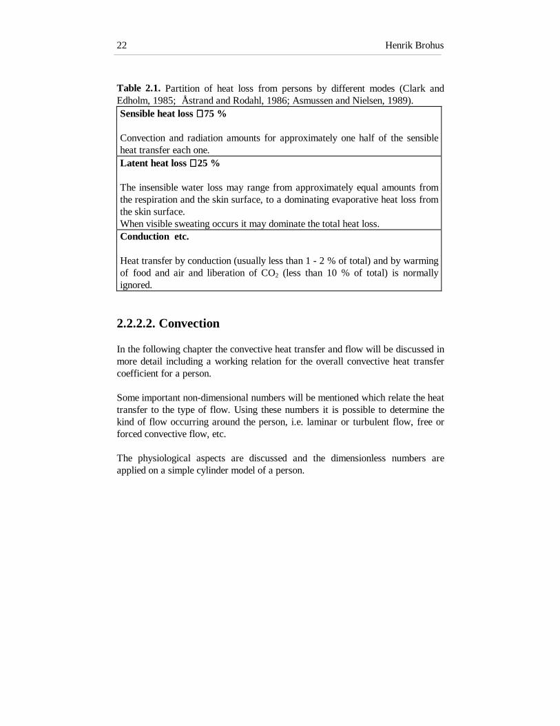
Henrik Brohus22
Table 2.1. Partition of heat loss from persons by different modes (Clark andEdholm, 1985; Åstrand and Rodahl, 1986; Asmussen and Nielsen, 1989).Sensible heat loss ∼∼∼∼ 75 %
Convection and radiation amounts for approximately one half of the sensibleheat transfer each one.Latent heat loss ∼∼∼∼ 25 %
The insensible water loss may range from approximately equal amounts fromthe respiration and the skin surface, to a dominating evaporative heat loss fromthe skin surface.When visible sweating occurs it may dominate the total heat loss.Conduction etc.
Heat transfer by conduction (usually less than 1 - 2 % of total) and by warmingof food and air and liberation of CO2 (less than 10 % of total) is normallyignored.
2.2.2.2. Convection
In the following chapter the convective heat transfer and flow will be discussed inmore detail including a working relation for the overall convective heat transfercoefficient for a person.
Some important non-dimensional numbers will be mentioned which relate the heattransfer to the type of flow. Using these numbers it is possible to determine thekind of flow occurring around the person, i.e. laminar or turbulent flow, free orforced convective flow, etc.
The physiological aspects are discussed and the dimensionless numbers areapplied on a simple cylinder model of a person.

Chapter 2 Tools for personal exposure assessment 23
Free convection
The convective heat transfer may be expressed as
( )C h t tc s a= − (2.5)
where
C = Rate of convective heat transfer (W/m2)hc = Convective heat transfer coefficient (W/m2°C)ts = Skin temperature (or surface temperature of clothing) (°C)ta = Ambient temperature (°C)
Even though the convection seems to be proportional to the temperature differencein the above formula it happens to be non-linear because the coefficient, hc,depends on the temperature difference itself. Apart from the temperaturedifference, hc also depends on the type of flow. This dependence may beexpressed by means of non-dimensional numbers.
The variables describing a certain physical problem (in this case the flow arounda person) may be numerous. By application of dimensional analysis thesedependent variables are combined in a few non-dimensional groups.
The convective heat transfer coefficient is part of the Nusselt number which maybe thought of as a dimensionless group incorporating this quantity indimensionless form
Nuh L
kc= (2.6)
where
Nu = Nusselt number (n.d.)L = Characteristic length (m)k = Thermal conductivity of the surrounding fluid (W/m°C)
In usual indoor environments where people are present the ambient airtemperature will be lower than the temperature of the skin or the clothing. The airwhich is in close contact with the person will thus be heated by conduction.

Henrik Brohus24
Due to the buoyancy of the warm air it will ascent along the entire person creatinga natural convection boundary layer.
The flow is termed as free convection if not disturbed by a dominating flow fieldin the surroundings.
The mathematical expression governing the free convection flow is the Grashofnumber, Gr. In the application of a person Gr may be written as (Clark and Toy,1975a)
( )Gr
gH T T
Ts a
a
=−3
2ν (2.7)
where
Gr = Grashof number (n.d.)g = Gravitational acceleration (9.82 m/s2)H = Vertical height of the body (m)ν = Kinematic viscosity (m2/s)Ts = Absolute temperature of the skin (K)Ta = Absolute temperature of the ambient air (K)
The Grashof number is proportional to the ratio of the buoyancy to the viscousforces within the air flow. The size of Gr determines the characteristics of theflow (Clark and Edholm, 1985)
Gr < 109 Laminar flow
Gr > 1010 Turbulent flow
As will be shown later, it is possible for the boundary layer flow to remainlaminar over the entire height of the person, especially if the person is clothed.
Apart from Gr the free convection heat transfer is governed by the Prandtlnumber
Pr = =c
kpµ ν
α (2.8)
where

Chapter 2 Tools for personal exposure assessment 25
Pr = Prandtl number (n.d.)cp = Specific heat of ambient air at constant pressure (J/kg°C)µ = Dynamic viscosity (kg/m s)k = Thermal conductivity (W/m°C)ν = Kinematic viscosity (m2/s)α = Thermal diffusivity (m2/s)
The Prandtl number is a physical property of the fluid itself related to the relativerates of transport of momentum and energy by the elements of the fluid. Thekinematic viscosity, ν, determines the way in which momentum is transferredacross a velocity gradient, and the thermal diffusivity, α, determines the way inwhich heat is transferred across a temperature gradient, thus Pr connects themomentum transfer with the heat transfer.
It can be shown by using dimensional analysis that during free convection thethree dimensionless groups mentioned earlier are related by the expression(Holman, 1989)
Nu Grfreem n∝ Pr (2.9)
In the usual range of applications Pr is approximately constant, i.e.
Nu a Grfreen= ⋅ (2.10)
Here, a and n may be determined empirically by means of measurements onpersons or by using an approximation where the person is simulated by a heatedcylinder which is not too slender.
Forced convection
If a person is exposed to a velocity field where the speed is considerable the flowmay change into forced convection. In case of forced convection the convectiveheat transfer coefficient does not depend on a temperature difference between theskin and the environment. The flow depends on the Reynolds number, Re, whichis proportional to the ratio of fluid inertial forces to viscous forces.

Henrik Brohus26
Re=UDν
(2.11)
where
Re = Reynolds number (n.d.)U = Free stream velocity (m/s)D = Characteristic length (m)ν = Kinematic viscosity (m2/s)
The size of Re determines whether the flow is laminar or turbulent (Schlichting,1979; Clark and Edholm, 1985)
Re < 2⋅105 Laminar flow
Re > 2⋅105 Turbulent flow
Here, the characteristic length, D, in Re is taken as the diameter of a cylinder withthe same height and the same surface area as a person.
The convective heat transfer coefficient incorporated in Nu may be determined as(Holman, 1989)
Nuforcedm n∝ Pr Re (2.12)
and as Pr is approximately constant
Nu aforcedn= ⋅ Re (2.13)
for smooth cylinders in normal air environments. If the characteristic length in Nuand Re is termed L, we have
h L
ka
U Lcn n
n=ν
(2.14)
and thus

Chapter 2 Tools for personal exposure assessment 27
hakL
U b Uc
n
nn n= ≅ ⋅
−1
ν(2.15)
where b may vary in general but will be constant for a fixed L and a fixedenvironment. A number of different working relations for hc exist (see e.g.ASHRAE, 1993), for instance
hc = 4.0 0 m/s < U < 0.15 m/s (2.16)
hc = 14.8⋅U0.69 0.15 m/s < U < 1.5 m/s (2.17)
which are valid for a standing person in moving air.
The hc above is the overall convective heat transfer coefficient. The localcoefficient may vary both with respect to the height and also around thecircumference of the body. For instance, Clark and Toy (1975b) measured thelocal convective heat transfer coefficient around the head, see Figure 2.2.
0
5
10
15
20
0 90 180 270 360
Angle to wind direction (degrees)
hc (
W/m
2 °C)
Figure 2.2. Variation of the local convective heat transfer coefficient hc
(W/m2°C) from the head with the angle, θ, to the flow in an air stream of 0.8 m/s.Reproduced from Clark and Toy, 1975b.
Henrik Brohus28
The above dependence of the angle shows a very close agreement with the flowaround a cylinder (Holman, 1989).
The local convective heat transfer coefficient may vary highly in vertical directionin case of free convection due to the development of the boundary layer thickness.For instance, Murakami et al. (1995) found a local hc - variation between 2W/m2°C (upper part) and 7 W/m2°C (at the feet) for a computer simulated personstanding in a stagnant flow, see also Appendix C.
Mixed free and forced convection
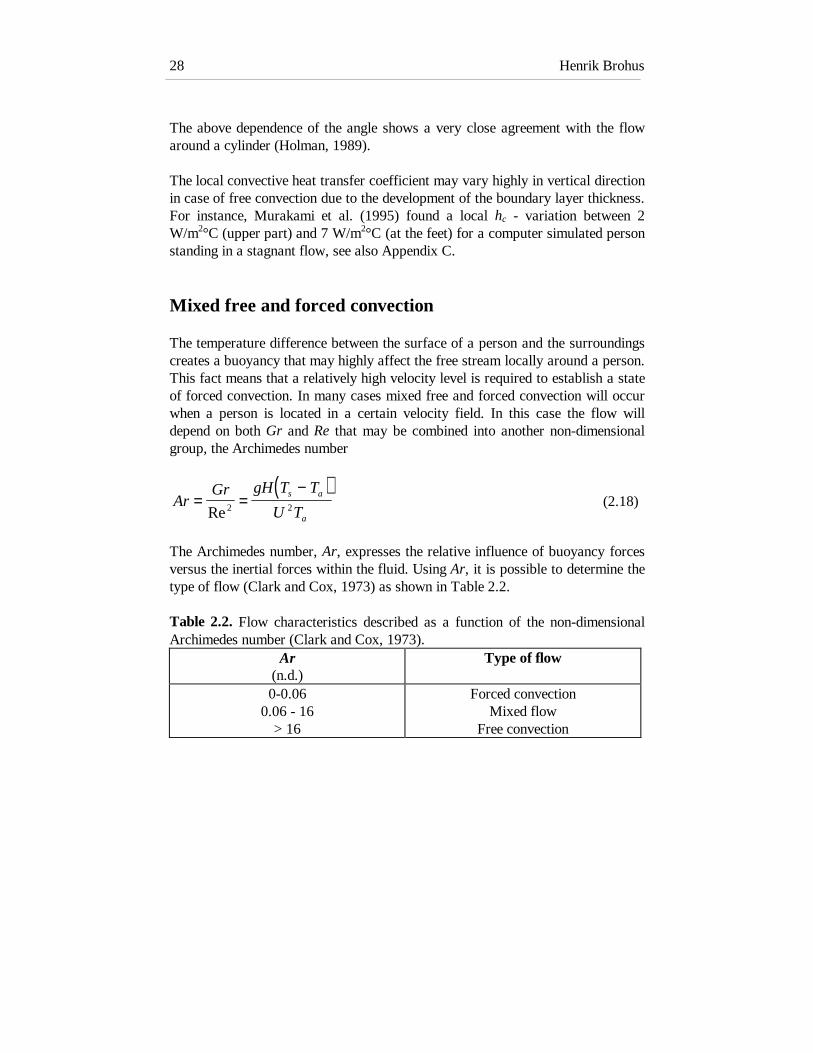
The temperature difference between the surface of a person and the surroundingscreates a buoyancy that may highly affect the free stream locally around a person.This fact means that a relatively high velocity level is required to establish a stateof forced convection. In many cases mixed free and forced convection will occurwhen a person is located in a certain velocity field. In this case the flow willdepend on both Gr and Re that may be combined into another non-dimensionalgroup, the Archimedes number
( )Ar
Gr gH T T
U Ts a
a
= =−
Re2 2 (2.18)
The Archimedes number, Ar, expresses the relative influence of buoyancy forcesversus the inertial forces within the fluid. Using Ar, it is possible to determine thetype of flow (Clark and Cox, 1973) as shown in Table 2.2.
Table 2.2. Flow characteristics described as a function of the non-dimensionalArchimedes number (Clark and Cox, 1973).
Ar(n.d.)
Type of flow
0-0.060.06 - 16
> 16
Forced convectionMixed flow
Free convection

Chapter 2 Tools for personal exposure assessment 29
Some physiological aspects
In many cases it is possible to simulate the body heat loss by using a uniformlyheated model, for instance, a cylinder where the heat loss continues to rise withincreasing air speed. However, the thermoregulatory mechanisms of the humanbody can alter the heat loss by changing the surface temperature. This may bedone by varying the blood supply to the skin, and also by changing the latent heatloss (sweating and water diffusion through the skin).
Clark and Edholm (1985) showed some local heat loss measurements on a personwhere the heat loss reached a maximum value and then began to decrease, eventhough the wind speed was increased.
Another physiological parameter that may act differently on a human being thanon a heated model is the effect of movements. When a person walks or runs onlythe head and the trunk move in a linear or unidirectional fashion. The upper armsand thighs perform a “pendulum” motion and the forearms and lower legs have awhiplash movement (Clark and Edholm, 1985).
This “pendulum” movements produce a different air flow pattern from the onefound assuming a uniform translation during movements. Clark and Edholm(1985) suggest that the convective heat transfer coefficient for the swinging partsshould be increased by a factor of approximately 2 compared with uniformtranslation.
Cylinder model of person
To give an example on the usage of the above-mentioned dimensionless numbers,a cylinder model of a person is applied in the following. This also gives an idea ofthe characteristics of the flow around the person including the influence ofdifferent insulation values of the clothing.

Henrik Brohus30
Figure 2.3. Cylinder model of an average sized person.
In Figure 2.3. the cylinder model of an average sized person is shown. The heightis 1.73 m and the weight is 70 kg corresponding to a surface area of 1.8 m2
(ASHRAE, 1993). The person is modelled by a cylinder with a height of 1.73 mand a diameter of 0.3 m.
The Reynolds number may be found if the cylinder diameter is taken as thecharacteristic length and the temperature of the ambient air is 20°C.
Re.
.= =
⋅⋅
≅ ⋅ ⋅−
UD UU
ν03
1511 102 106
4 (2.19)
For Re = 2⋅105 the flow around the person (cylinder) is turbulent which in thiscase corresponds to a free stream velocity of 10 m/s, i.e. well above velocitiesobtained in usual indoor environments.
If the surroundings are quiescent we may determine the kind of flow in the naturalconvection boundary layer along the person by means of the Grashof number.This is done for three different cases corresponding to different thermal insulationvalues of the clothes.
For a naked person (Icl = 0 clo) the skin temperature is taken as 33.7 °C which isthe “neutral value” obtained when the body maintains its thermal equilibrium withthe environment with minimum regulatory effect (ASHRAE, 1993). Using this

Chapter 2 Tools for personal exposure assessment 31
skin temperature it is possible to calculate the surface temperature of the clothing,tcl, for a certain insulation value of the clothes, Icl, see Appendix A. For typicallyindoor summer clothes (Icl = 0.5 clo), tcl = 29.8°C, and for a typically indoorwinter clothes (Icl = 1.0), tcl = 26.0°C. If the ambient air temperature is kept at20°C the following relationship between the local Grashof number and thevertical distance is found for the three cases, see Figure 2.4.
Figure 2.4. Vertical variation of the local Grashof number, Gr, for a person insurroundings of 20°C when the person is naked (0 clo), wearing summer clothes(0.5 clo) and wearing winter clothes (1.0 clo). When Gr < 109 the flow islaminar, and when Gr > 1010 the flow is turbulent which is indicated by the twovertical lines.
In Table 2.3. the Archimedes number, Ar, is used to estimate the velocity level ofa uniform free stream around a person necessary to achieve a certain type of flow.The results in Table 2.3. are based on a calculation of the free stream velocity, U,for a person with a height of 1.73 m standing in surroundings of 20°C. When Ar< 0.06 the flow is forced convection and when Ar > 16 the flow around the personis free convection.
���������������������������������������������
������������������������������
0
1
2
1.0E+07 1.0E+08 1.0E+09 1.0E+10
Local Grashof number (n.d.)
Ver
tical
dis
tanc
e (m
) 1.0 clo
0.5 clo
0 clo

Henrik Brohus32
The velocity levels obtained for the free convection case correspond well withmeasurements and observations by Brohus and Nielsen (1994a) and Hyldgaard(1994).
Table 2.3. Uniform free stream velocity, U, necessary to obtain free convectionand forced convection around a person, respectively, for three insulation values ofthe clothing. When the velocity level is found between the two flow typesmentioned in the table, the flow is termed mixed free and forced convection.
Uniform free stream velocity around a person, UType of convective flow
Clothing insulation(clo)
Free(m/s)
Forced(m/s)
00.51.0
0.220.190.15
3.643.082.40
2.2.2.3. Radiation
Radiative heat loss from persons may be found by using an application of theStefan-Boltzmann equation for radiative heat transfer.
The surface area of naked persons should be turned into an effective radiationarea, i.e. the area of the person actually exposed to the radiation. This area shouldalso consider the effect of clothing.
A f f Aeff eff cl Du= (2.20)
where
Aeff = Effective radiation area (m2)ADu = DuBois area (naked surface area of the person) (m2)feff = Effective radiation area factor (n.d.)fcl = Clothing area factor (n.d.)
Fanger (1972) found the effective radiation area factor, feff, to be 0.696 forsedentary body position and 0.725 for a standing person. The clothing area factor,fcl, can be found by (McCullough et al., 1989)

Chapter 2 Tools for personal exposure assessment 33
fA
AIcl
cl
Ducl= = +1 03. (2.21)
where
Acl = Clothed surface area (m2)Icl = Clothing insulation (clo)
The radiative heat loss may then be expressed as
[ ]Φ r eff s rA T T= −εσ 4 4 (2.22)
where
Φr = Radiative heat loss (W)ε = Average emissivity of clothing and body area (n.d.)σ = Stefan-Boltzmann constant (5.669⋅10-8 W/m2K4)Ts = Absolute skin temperature (K)Tr = Absolute mean radiant temperature (K)
The emittance, ε, for human skin is close to 1.0, and since most types of clothinghave emittances of 0.95 it is suggested to use the mean value of 0.97 (Fanger,1972).
The mean radiant temperature is the uniform temperature of an imaginaryenclosure (black surroundings), in which radiant heat transfer from the humanbody equals the radiant heat transfer in the actual non-uniform enclosure(ASHRAE, 1993).
Most building materials have high emittance, therefore, it is usually assumed thatthe surrounding surfaces act as black bodies, i.e.
T T F T F T Fr P P N P N4
14
1 24
24= + + +− − −� (2.23)
where
Tr = Absolute mean radiant temperature (K)
TN = Absolute surface temperature of surface N (K)

Henrik Brohus34
FP-N = Angle factor between a person and surface N (n.d.)
If the mutual temperature differences of the surfaces are relatively small theabove equation may be simplified to a linear form (ASHRAE, 1993)
t t F t F t Fr P P N P N= + + +− − −1 1 2 2 � (2.24)
where the temperature unit is °C in this expression. The above formula assumesthat reflections between the surfaces can be disregarded. If this is not the case theradiosity of the surfaces should be used in calculating Tr (Holman, 1989), which
will complicate the calculation extensively.
Radiative heat loss from persons may also be expressed in a linearized form usingthe radiative heat transfer coefficient in the same manner as the convective heattransfer coefficient (ASHRAE, 1993)
( )R f h t tcl r cl r= − (2.25)
where
R = Radiative heat transfer (W/m2 outer surface of clothed body)hr = Linear radiative heat transfer coefficient (W/m2°C)tcl = Mean temperature of outer surface of the clothed body (°C)t r = Mean radiant temperature (°C)
and
h ft t
r effcl r= +
+
4 273152
3
εσ . (2.26)
Magnitude of the radiative heat transfer coefficient
As for the convective heat transfer coefficient in the preceding chapter, theradiative heat transfer coefficient is calculated for an environment of 20°C to givean idea of the order of magnitude for three different levels of clothing insulation,see Table 2.4.

Chapter 2 Tools for personal exposure assessment 35
Table 2.4. Example of the linear radiative heat transfer coefficient for a standingperson in surroundings with a mean radiant temperature of 20°C for threedifferent cases corresponding to a naked person (0 clo), typically summer clothes(0.5 clo), and typically winter clothes (1.0 clo). ε = 0.97 and feff = 0.725. Thecalculation of tcl is described in Appendix A.
Radiative heat transfer coefficientClothing insulation
(clo)tcl
(°C)hr
(W/m2°C)0
0.51.0
33.729.826.0
4.34.24.1
2.2.3. Respiration
In Chapter 1 it was mentioned that the route for personal exposure examined inthe present work is exposure via the respiration. Therefore, a short introduction tothe respiratory system will be given in the subsequent chapter, including aformula used for the calculation of the pulmonary ventilation which is necessaryfor the assessment of the dose, see Chapter 1.
The living cells in the human body use oxygen for its metabolism, and as a resultof this process carbon dioxide is produced. Two transport systems are used tocarry the O2 and the CO2 between the cells and the environment surrounding theperson: a circulatory system supplies the blood and a respiratory system suppliesair to the lungs. Thus, the main function of the respiratory system is to provideoxygen to the cells of the body and to remove excess carbon dioxide (Turiel,1985).
The pulmonary airways consist of three different parts, see Figure 2.5. First, theupper airways, extending from the nares and the lips to the larynx. Here, the air iswarmed and moistened. Secondly, the conducting airways where the air isdistributed in the lungs in a branched-tube network starting at the trachea andextending to include the terminal bronchioles. Third, the respiratory zone thatbegins with the respiratory bronchioles and ends with the alveoli (little air sacs).Here, the gas exchange takes place (Ultman, 1988).

Henrik Brohus36
Figure 2.5. Major anatomical features of the human respiratory system.Reference: Turiel, 1985.
The state of the air in the lungs is 37°C and 100% rh at barometric pressure,while the exhaled air in usual surroundings is approximately 34°C and 100% rh(see also Appendix A).
The pulmonary ventilation is defined as the volume of air which is exhaled perminute. By definition the pulmonary ventilation equals the frequency ofrespiration multiplied by the mean expired volume (Åstrand and Rodahl, 1986)
�V f Vres res T= ⋅ (2.27)
where
�Vres = Pulmonary ventilation (litre/min)
fres = Frequency of respiration (min-1)VT = Mean expired tidal volume (litre)
At rest the frequency of respiration is 10 - 20 min-1 and increasing depending onthe activity level of the person. For well trained athletes 60 min-1 is not unusual.The pulmonary ventilation at rest is about 6 litre/min increasing according to theactivity level up to 200 litre/min in the extreme case (Åstrand and Rodahl, 1986).

Chapter 2 Tools for personal exposure assessment 37
In Table 2.5. examples of typical levels of the three above mentioned parametersare shown for different activity levels.
Table 2.5. Examples on tidal volume, frequency of respiration and pulmonaryventilation for different activity levels (Asmussen and Nielsen, 1989).
Activity level Tidal volume(litre)
Frequency(min-1)
Pulmonaryventilation(litre/min)
RestModerate workMaximal work
0.5~ 2.5~ 3.0
1212
30 - 40
630
90 - 120
According to ASHRAE (1993) the pulmonary ventilation may be expressed as afunction of the activity level as follows
�m K Mres res= ⋅ (2.28)
where
�mres = Pulmonary ventilation rate (kg/s)
Kres = Constant (2.58⋅10-6 kg m2/J)M = Rate of metabolic heat production (activity level) (W/m2)
If it is assumed that the temperature of the expired air is 34°C, �mres in kg/s may
be converted into �Vres in litre/min, i.e.
� .V K M Mres res= ′ ⋅ = ⋅01348 (2.29)
where
�Vres = Pulmonary ventilation (litre/min)
Kres' = Constant (0.1348 litre m2 / W min)
M = Rate of metabolic heat production (activity level) (W/m2)

Henrik Brohus38
2.2.4. Description of the Breathing Thermal Manikin
2.2.4.1. Introduction
An extensive number of different physical models of human beings have beenused in research for various purposes. Table 2.6. gives an overview of the topic.
Table 2.6. Overview of characteristics and purpose for different physical modelsof a human being.Physical models of human beingsFeatures:
- Geometry (anatomically correct, small-scale, cylinder, cuboid, sphere, etc.)- Posture (standing, seated, lying, movements)- Heating (none, surface temperature, heat flux, etc.)- Respiration (none, exhaust from point, artificial lung, etc.)- Etc.
Purpose:
- Thermal insulation of clothing- Heat transfer coefficients- Flow characteristics around the body- Thermal comfort- Personal exposure- Source of heat, contamination and momentum- Interaction between persons- Etc.
The main interest in the present work is physical models of humans used fordetermination of personal exposure. The models used for this purpose mayroughly be divided in three different categories:

Chapter 2 Tools for personal exposure assessment 39
1. Heated cylinders (e.g. Nickel et al., 1990; Holmberg et al., 1990; Stymne et al.,1991; Mattsson and Sandberg, 1994; Krühne and Fitzner, 1994).
2. Unheated, anatomically correct, small-scale models (e.g. Fletcher and Johnson,1988; Flynn and Shelton, 1990; George et al., 1990; Flynn and George, 1991;Kim and Flynn, 1991a, 1991b, 1992).
3. Heated, anatomically correct, full-scale models with respiration (e.g. Clark andCox, 1973; Säteri, 1992a, 1992b; Brohus and Nielsen, 1994a; 1995; 1996b;Rodes et al., 1995; Bjørn and Nielsen, 1996a; b).
The physical models of a human being used in the present work belong to thethird category, i.e. the Breathing Thermal Manikin shown in Figure 2.7.
2.2.4.2. Construction of manikin
The Breathing Thermal Manikin (BTM) is developed at the Thermal InsulationLaboratory, Technical University of Denmark. The BTM is shaped as a 1.7 mhigh average sized woman, developed from a nearly anatomically correct femaledisplay manikin consisting of a 4 mm fibreglass-armed polyester shell. The shellis wound with nickel wire of 0.3 mm in diameter at a maximum spacing of 2 mm,see Figure 2.6. The wire is used sequentially both for the heating of the manikinand for measuring and controlling the skin temperature. Outside the wiring aprotective shield is placed with a thickness less than 1 mm.
The manikin is divided in 16 parts, and it is supplied with joints in shoulders, hipsand knees. This enables it to stand, sit and to move, e.g. on a bicycle (with theenergy of movements supplied from outside). The different surface areas of theindividual parts can be found in Appendix B.

Henrik Brohus40
Figure 2.6. The Breathing Thermal Manikin under construction at the TechnicalUniversity of Denmark. Here, the resistance wire used for heating, measuring andcontrolling the skin temperature and the heat output is mounted on the head.
The BTM is controlled to obtain a skin temperature and a heat outputcorresponding to people in thermal comfort. Fanger (1972) found a relationshipbetween the skin temperature and the total heat output necessary to achievethermal comfort. However, due to the fact that the manikin is not able toevaporate moisture the sensible heat loss is used in stead of the total heat loss.Therefore, the following relationship between the skin temperature, ts, and thesensible heat output, Qt, is derived and used for the control (Tanabe et al., 1994).The full derivation is found in Appendix A.
t Qs t= − ⋅36 4 0 054. . (2.30)
Each of the 16 parts of the body is equipped with individual systems for heatingand control. The control circuit is designed as a proportional control system witha set-point of 36.4 °C and a load error of 0.054 m2°C/W. The load error will reactas a thermal resistance equal to the resistance between the skin and the deep body.

Chapter 2 Tools for personal exposure assessment 41
The skin temperature is measured in the range of 18°C - 37°C with a resolution of0.1°C and a maximum heat loss of 140 W/m2. The BTM is calibrated in thelaboratory by the author to an uncertainty of ± 0.2°C.
Figure 2.7. Breathing Thermal Manikin used to measure the personal exposure.The manikin is separated in 16 individual parts of the body, each with the samesurface temperature and heat output as people in thermal comfort. The manikinhas an artificial lung to simulate breathing. Height = 1.7 m, ADu = 1.5 m2, Icl = 0.8clo.
The control and the function of the manikin are verified by measuring theconvective heat transfer coefficient among other things, see Appendix C.

Henrik Brohus42
The BTM is wearing tight-fitting clothes with an insulation value, Icl, of 0.8 clo.This value corresponds well to typical indoor clothing insulation which is usuallyfound in the interval between 0.5 clo and 1.0 clo. In Appendix D measurements ofthe clothing insulation are reported.
Tight-fitting clothes are chosen instead of loose-fitting clothes where the localsurface temperatures, heat transfer and thus the flow field may changesignificantly due to large variations in the location of insulating enclosures ofstagnant air. The choice of tight-fitting clothes results in more consistent andreproducible measurements.
Respiration is simulated by means of an artificial lung which is able to providethe breathing either through the mouth or through the nose. It is possible to adjustboth the frequency of respiration (number of breaths per minute) in the range of 3- 30 min-1 and the pulmonary ventilation (litre per minute) in the range of 5 - 18litre/min.
In this work 10 min-1 is chosen as the frequency of respiration and 10 litre/min asthe pulmonary ventilation. The respiration is performed through the mouth.
2.2.5. Personal exposure assessment using the BTM
Due to the fact that the Breathing Thermal Manikin is equipped with both anartificial lung and the possibility to breathe either through the mouth or the nose,it is relatively easy to determine the personal exposure by analysing a sample ofsubstance which is actually inhaled, according to the definition of personalexposure in Chapter 1.
In the present work only gaseous contaminants are considered. The transport ofcontaminant is modelled by means of tracer gas which is assumed to simulate thebehaviour of a gaseous contaminant source satisfactory.
Nitrous oxide (N2O) is used as tracer gas. However, the gas has a densityapproximately 1.5 times higher than atmospheric air, which is found to influencethe dispersion pattern substantially, especially in case of quiescent surroundings.

Chapter 2 Tools for personal exposure assessment 43
To eliminate that problem the tracer gas is mixed with the lighter helium (He) toobtain a mixture which is density neutral compared with the density of thesurrounding air.
The tracer gas concentration is measured by means of photoacoustic spectroscopy(PAS). Here, a gas property is used, namely that the gas molecules can absorbcertain frequencies of infrared light, gain energy and vibrate more vigorously. Theexited molecules thus transform their extra energy to other molecules by collisionwhich causes increased molecular speed which finally results in a raisedtemperature of the gas.
When PAS is used a gas sample is collected in a measurement chamber. Thechamber is irradiated with pulsed (chopped) light. The gas absorbs lightproportional to its concentration and converts it into heat, quickly afterwards thegas cools again. The chopped light causes temperature fluctuations that generatespressure waves. Finally, the pressure waves are detected by a microphone.
In the present measurements a Brüel & Kjær 1302 Multi-gas Monitor is usedtogether with a Brüel & Kjær 1303 Multipoint Sampler and Doser. Theconcentration is measured by sampling with a frequency of approximately onesample per minute. The equipment is calibrated to an uncertainty of ± 2%,including cross calibration and water interference calibration.
2.3. Computer Simulated Person
2.3.1. Introduction
This Chapter 2.3. will present a numerical tool for personal exposure assessment,namely the Computer Simulated Person. Three different models are proposedranging from a heated cuboid to a model including “legs” and “head”.
First, the mathematical equations governing the fluid flow and the contaminanttransport processes are mentioned together with a description of the numericalsolution procedure and the treatment of selected boundary conditions.

Henrik Brohus44
Then the three different versions of the Computer Simulated Person (CSP) areintroduced and, finally, the procedure for personal exposure assessment using theCSP is discussed.
2.3.2. Computational Fluid Dynamics
2.3.2.1. Governing equations
The aim of Computational Fluid Dynamics (CFD) is to provide a numericalsolution of the mathematical equations governing fluid flow and related physicalprocesses. The description of fluid dynamics will often include the topics of heattransfer, mass transfer and very often also turbulence modelling etc.
The set of equations actually involved and the appearance of the specific terms inthe equations depend on the case of interest due to different assumptions andpossible simplifications. For instance, it makes a difference whether the flow isisothermal or not, compressible or incompressible, etc.
In this work only steady-state problems will be considered. The flow is assumedto be three-dimensional, incompressible, non-isothermal and turbulent (orlaminar). To account for the dispersion of contaminant and thus personalexposure an equation for the transport of contaminant (mass) must be included.This leads to the following set of governing equations.
Continuity equation
One of the basic laws in fluid motion, conservation of mass, is derived by meansof a mass balance for a control volume in the fluid where the incoming mass flowequals the outgoing mass flow (incompressible fluid), in cartesian tensor notationthe continuity equation is
( )∂ ρ∂
u
xi
i
= 0 (2.31)

Chapter 2 Tools for personal exposure assessment 45
where
ρ = Density of the fluid (kg/m3)ui = Mean velocity component corresponding to the i direction (m/s)xi = Co-ordinate direction i (m)
Navier-Stokes equations
The Navier-Stokes equations, which are also termed the momentum equations, areexpressing Newton’s second law of motion for the fluid, i.e. the transport andconservation of momentum. The equations are derived by applying Newton’ssecond law on a fluid element influenced by surface forces (shear stresses andpressure) and volume forces (buoyancy)
( )∂ ρ∂
∂∂
µ∂∂
∂∂
ρ∂∂
u u
x x
u
x
u
xu u
p
xB S
i j
j jl
i
j
j
ii j
ii u= +
−
− + +' ' (2.32)
where
p = Pressure (N/m2 or Pa)µl = Laminar dynamic viscosity (kg/m s)ui′ = Fluctuating velocity component in the i direction (m/s)Bi = Volume force in the i direction (N/m3)Su = Source term (N/m3)
The term on the left side, the convection term, expresses the net supply ofmomentum from the surroundings. First term on the right side, the diffusion term,expresses the influence from the shear forces. Second term is the pressuregradient term which is due to the normal forces and, finally, the buoyancy termwhich accounts for the volume forces acting on the fluid and the source termwhich is frequently used to implement the boundary conditions.
In the diffusion term the quantity − ρu ui j' ' is called the Reynolds stresses (or
additional stresses) and they result from taking the instantaneous equations intomean equations (Rodi, 1980). The physical meaning of the Reynolds stresses isthe effect of the turbulent transport of fluid across the main flow direction, whichinfluences the flow in the same way as increased shear stress.

Henrik Brohus46
The various turbulence models are making assumptions for the Reynolds stressesfor the closure of the mean equation. In the present work the eddy viscosityconcept is used. Here, the turbulent stresses are assumed to be proportional to thegradient of the mean velocity and the turbulence is assumed to be isotropic (Rodi,1980), i.e.
− = +
−ρ µ
∂∂
∂∂
ρ δu uu
x
u
xki j t
i
j
j
iij' '
2
3(2.33)
where
µt = Turbulent viscosity (eddy viscosity) (kg/m s)k = Turbulent kinetic energy (J/kg)δij = Kronecker delta (equals 1 for i = j and equals 0 for i ≠ j)
In that way an effective viscosity, µeff, can be defined as the sum of the laminarand the turbulent viscosity
µ µ µeff l t= + (2.34)
It is important to acknowledge the differences between the laminar and theturbulent viscosity. While the laminar dynamic viscosity, µl, is a constant for aspecific fluid, the turbulent viscosity, µt, depends on the flow, and it may varyhighly throughout the flow domain. µt is found by means of a turbulence model.
The last term in the expression of the Reynolds stresses must be included to beconsistent with the subsequent definition of the turbulent kinetic energy, k. Theterm expresses the normal stresses, i.e. when i = j, in which case the first term onthe right side is zero according to the continuity equation. These normal stressesact like pressure forces and, therefore, they are sometimes included in the pressuregradient term as an “effective” pressure p + 2/3 k (Rodi, 1980). This last term,however, is often small for what reason it is frequently ignored in the numericalscheme.
The buoyancy term, Bi, may be described as follows, using the Boussinesqapproximation (Arpaci and Larsen, 1984)

Chapter 2 Tools for personal exposure assessment 47
( )B g t ti i ref= − −ρβ (2.35)
where
β = Coefficient of cubic expansion (1/K)gi = Gravitational acceleration in the i direction (m/s2)t = Temperature of the fluid (°C)tref = Reference temperature (°C)
Inserting the above expressions for the Reynolds stresses and for the buoyancyterm in the Navier-Stokes equations results in
( ) ( )∂ ρ∂
∂∂
µ∂∂
∂∂
∂∂
ρβu u
x x
u
x
u
x
p
xg t t S
i j
j jeff
i
j
j
i ii ref u= +
− − − + (2.36)
Energy equation
To obtain a description of the temperature distribution throughout the non-isothermal flow domain the energy equation is used. This equation is derived fromthe basic law of conservation of energy, i.e. the first law of thermodynamicsapplied on a fluid element assuming that the fluid is acting as a perfect gas
( )∂ ρ
∂∂
∂λ
∂∂
c u t
x x
t
xS
p j
j jeff
jt=
+ (2.37)
where
ρ = Density of the fluid (kg/m3)cp = Specific heat at constant pressure (J/kg°C)t = Mean temperature of the fluid (°C)λeff = Effective conductivity (W/m°C)St = Source term (W/m3)

Henrik Brohus48
The source term, St, includes eventual heat sources and sinks. The effectiveconductivity, λeff, is expressed as
λ λ λeff l t= + (2.38)
where
λl = Laminar thermal conductivity (W/m°C)λt = Turbulent conductivity (W/m°C)
The laminar thermal conductivity, λl, is a fluid property that is constantthroughout the domain, whereas the turbulent conductivity, λt, depends on thelocal flow field in the same way as µt. λt is usually found by means of theturbulent Prandtl number, σt, in an analogy between the transfer of energy andmomentum
σνα
µλt
t
t
p t
t
c= = (2.39)
where
σt = Turbulent Prandtl number (n.d.)νt = Turbulent kinetic viscosity (m2/s)αt = Turbulent thermal diffusivity (m2/s)
The turbulent kinetic viscosity, νt, of the fluid conveys information about the rateof which momentum may diffuse through the fluid because of turbulent motion(stresses). The turbulent thermal diffusivity, αt, explains the same thing in regardto the diffusion of heat, i.e. thermal energy, in the fluid. The turbulent Prandtlnumber is thus the connecting link between the velocity field and the temperaturefield. It is usually considered to be constant and close to unity, in this work it willbeσ t = 09. .

Chapter 2 Tools for personal exposure assessment 49
Concentration equation
As mentioned previously an additional equation is required to calculate thedispersion and transport of a gaseous contaminant. This equation, theconcentration equation, is based on mass conservation
( )∂∂
∂∂
∂∂
u c
x xD
c
xS
j
j jeff
jc=
+ (2.40)
where
c = Concentration of contaminant (kg of species / kg of air)Deff = Effective diffusivity (m2/s)Sc = Source term (kg of species / kg of air ⋅ s)
The concentration, c, may easily be converted into the unit of mg/m3 or ppmwhere it is convenient. The effective diffusivity, Deff, is defined as
D D Deff l t= + (2.41)
where
Dl = Mass molecular diffusivity (m2/s)Dt = Turbulent diffusivity (m2/s)
The turbulent diffusivity is found by means of a turbulent Schmidt number forconcentration, σc, analogue to the turbulent Prandtl number for the energyequation
σν
ct
tD= = 09. (2.42)
Turbulence model
In order to describe the turbulent viscosity (eddy viscosity), µt, the followingrelation is used (Rodi, 1980)

Henrik Brohus50
µ ρεµt ck
=2
(2.43)
where
µt = Turbulent viscosity (kg/m s)ρ = Density of the fluid (kg/m3)cµ = Constant (= 0.09) (n.d.)k = Turbulent kinetic energy (J/kg)ε = Rate of dissipation of turbulent kinetic energy (J/kg s)
The turbulent kinetic energy, k, and the rate of dissipation of turbulent kineticenergy, ε, are defined as (Abbott and Basco, 1989)
k u ui i≡1
2' ' (2.44)
ε ν≡ −2 s sij ij (2.45)
where sij is the strain rate of the fluctuating flow (s-1)
su
x
u
xiji
j
j
i
≡ +
1
2
∂∂
∂∂
' '(2.46)
and ui′ is the fluctuating component of the instantaneous velocity in the i direction(m/s).
The above expression for µt is derived on the basis of dimensional analysis andconsiderations of the velocity and length scales in the flow, assuming that there isa constant rate of energy transfer from the largest energy containing eddies to thedissipative small structures of the flow. Two additional partial differentialequations are required for k and ε to close the set of equations, see Appendix E.

Chapter 2 Tools for personal exposure assessment 51
General form of equations
It is possible to write the equations in a more general form facilitating thediscretisation and the solution. If the dependent variable is denoted φ, a diffusioncoefficient is denoted Γφ, and a source term Sφ the following form of thedifferential equations can be written which is more comprehensible for thediscretisation
( )∂ ρ φ∂
∂∂
∂φ∂φ φ
u
x x xS
j
j j j
=
+Γ (2.47)
with different meanings of φ, Γφ and Sφ according to the respective equations. Theleft term is the convection term, the first term on the right side is the diffusionterm and the last term is the source term.
2.3.2.2. Numerical solution of equations
Discretisation technique
Using the Finite Volume Method the calculation domain is divided into a finitenumber of control volumes and grid points, so that there is one volumesurrounding each grid point.
The differential equations are integrated over each control volume and piecewiseprofiles expressing the variation between the grid points are used to evaluate therequired integrals (Brohus, 1992; Nielsen, 1994).
The hybrid scheme, i.e. a combination of central difference and upwinddifference, is used in the evaluation of the convection terms (Patankar, 1980).
The source term, Sφ, is most often dependent on the variable φ. This dependence isdescribed in a linear form even though it may be non-linear.
Pressure is deduced indirectly from the continuity equation by using the SIMPLEalgorithm, for instance described by Patankar (1980).
Henrik Brohus52
After the discretisation a set of linear algebraic equations is obtained which canbe solved using standard solution techniques, e.g. the TriDiagonal-MatrixAlgorithm.
Non-linearities
Non-linearities are handled by iteration starting by guessing or estimating thevariables at all grid points. From these values and the boundary conditions thecoefficients in the discretized equations are calculated. Each of the coupledtransport equations is solved separately in linearized form. In that way new valuesof the concerned variable are obtained which can be used to calculate thecoefficients of the following equations and so on, until the convergence of theequations.
In the iterative solution of the algebraic equations, employed for handling the non-linearity, it is most often necessary to slow down the changes of a dependentvariable from iteration to iteration to avoid divergence. This process is calledunderrelaxation, and it is a very useful device for non-linear problems (Patankar,1980).
2.3.2.3. Boundary conditions
Due to the elliptic nature of the governing equations boundary conditions (BC)are required along all boundaries of the solution domain.
In the present CFD calculations several BC´s are used, for instance inlet opening,return opening, symmetry plane, wall functions for the description of friction andheat transfer etc. The last two will be explained in more detail in the subsequent.
The description is made in accordance with the formulas applied by Flovent(1994) to be consistent with the software used for the calculations.

Chapter 2 Tools for personal exposure assessment 53
Friction at the walls
When the fluid, i.e. the air in a ventilated room, is passing a wall the velocity inthe boundary layer is decreasing from “free stream” velocity level to zero velocityon the surface, the so called no slip condition. This process causes a surfacefriction which highly affects the flow field, especially close to the surface. Inorder to provide a satisfactory numerical description of this phenomenon it isnecessary to use a high number of grid points (control volumes) close to the walls.
Another approach that is used in this work is to employ wall functions in order toevaluate surface friction between the wall surface and the near-wall grid node.This approach will save a great number of grid points in the proximity of surfacesand, therefore, decrease the demand of computer power and CPU timeconsiderably.
Standard wall functions separate the boundary layer in two regimes, a viscoussub-layer and a fully turbulent region. The wall functions are based onmeasurements and calculations on a steady, turbulent channel flow (Arpaci andLarsen, 1984). This implies that the boundary layer along surfaces in the CFDsimulations is assumed to act as the boundary layer obtained in the case of achannel flow.
Two non-dimensional quantities are used in the description of the wall functions,namely a velocity, u+, and a length, y+ defined as (analogue to the velocities v+
and w+ and the length x+ and z+)
uu
u+ =
τ(2.48)
and
yyu+ =
ρµ
τ(2.49)
u wτ
τρ
= (2.50)

Henrik Brohus54
where
u+ = Dimensionless velocity (n.d.)u = Velocity in x direction (transversely to the y direction) (m/s)uτ = Friction velocity (m/s)τw = Wall shear stress (N/m2)y = Co-ordinate in y direction (m)y+ = Dimensionless length (n.d.)ρ = Density of fluid (kg/m3)µ = Laminar dynamic viscosity (kg/m s)
The non-dimensional distance from the wall, y+, can also be viewed as a localReynolds number, which clearly appears from the definition above.
For the laminar regime, i.e. the viscous sub-layer, we get for y+ ≤ 11.5 (Flovent,1994)
u y+ += (viscous sub-layer, laminar regime) (2.51)
and for the fully developed turbulent regime, for y+ > 11.5, we get the logarithmiclaw-of-the-wall
( )u y+ +=1
0 4359
.ln (turbulent region) (2.52)
In the numerical solution procedure the wall shear stress, τw, is deduced from theabove formulas by means of the calculated values of the velocity, u, in the firstgrid node at the distance, y, from the wall surface. This is straightforward in thelaminar case, while in the turbulent region it involves iteration. The wall shearstress is then applied as a negative source of momentum in the Navier-Stokesequations for the near-wall cell. In that way the no slip condition and the effect offriction are included in the CFD calculations.
Heat transfer at the walls
Two different boundary conditions are used to model heat transfer at the walls inthe CFD calculations.

Chapter 2 Tools for personal exposure assessment 55
The most simple and also the most exact and grid independent heat transfer BC isa direct prescription of the heat flux at the surface, e.g. in W/m2. This procedureshould be applied whenever possible.
Often, however, the applied BC regarding heat transfer at the walls is the surfacetemperature, tw. This raises a demand for the calculation of a local convectiveheat transfer coefficient to express the heat flow between the wall and the firstgrid node, i.e.
( )Q h t tc c p w= − (2.53)
where
Qc = Local convective heat transfer (W/m2)hc = Local convective heat transfer coefficient (W/m2°C)tp = Air temperature at the first grid node (°C)tw = Surface temperature at the wall (°C)
The heat transfer is determined by means of the non-dimensional Stanton number,St, which is an expression of the ratio of energy flux to momentum flux in thefluid
StNu h
c uc
p
= =Re Pr ρ
(2.54)
where
St = Stanton number (n.d.)Nu = Nusselt number (n.d.)Re = Reynolds number (n.d.)Pr = Prandtl number (n.d.)
If the Stanton number is known Qc may be found as
( )Q c u t t Stc p p w= −ρ (2.55)

Henrik Brohus56
As for the description of the wall friction the boundary layer is divided in tworegions. For the laminar flow, y+ ≤ 11.5, we obviously have
St=1
Re Pr(viscous sub-layer, laminar region) (2.56)
i.e.
( )Qy
t tcl
p w= −λ
(viscous sub-layer, laminar region) (2.57)
where λl is the laminar thermal conductivity of the flow.
In case of turbulent flow, where y+ > 11.5, St is found in an analogy between heatand momentum transfer. Assuming that the turbulent diffusivities are order ofmagnitudes larger than the molecular diffusivities, and that the turbulent Prandtlnumber is approximately equal to one the Reynolds analogy is obtained (Arpaciand Larsen, 1984)
St s= (2.58)
where
suw=
τρ 2 (2.59)
However, to include a possible variation of the Prandtl number the Prandtl-Taylorcorrection is applied in a generalised form, including the sub-layer resistancefunction by Jayatilleke (1969), (Patankar and Spalding, 1970)
( )Sts
P st j
=+σ 1
(turbulent region) (2.60)
and

Chapter 2 Tools for personal exposure assessment 57
Pjl
t
t
l
= −
9 1
1 4σσ
σσ
/
(2.61)
where
Pj = Jayatilleke´s sub-layer resistance function (n.d.)σl = Laminar Prandtl number (n.d.)σt = Turbulent Prandtl number (n.d.)
As mentioned in the previous paragraph σt = 0.9 is used. The laminar Prandtlnumber, σl, is close to 0.71 for room air at usual indoor conditions, i.e.
( )Sts
s=
−09 1 2.(room air, turbulent region) (2.62)
which is the relation used in the present CFD calculations for the turbulent region.
Consequently, when the heat transfer BC is the wall temperature and the flow isturbulent St may be found by means of u, τw (hence s) and tp. Qc is calculatedfrom the Stanton number and then applied as a heat source in the energy equationfor the affected near-wall cell.
Even though the boundary layer is separated in two regions, the solution dependson the choice of grid layout, both regarding the heat transfer BC where thesurface temperature is prescribed and also regarding the surface friction BC. Thistopic is discussed in more detail in Chapter 2.3.3.2.
2.3.2.4. Software
The equations and the numerical scheme mentioned above are implemented in thecommercial software product FLOVENT from Flomerics Ltd. This software hasbeen used to perform the CFD calculations presented here.
FLOVENT is a special-purpose CFD program which has been developed incollaboration between Flomerics Ltd. and BSRIA (The Building ServicesResearch and Information Association, Berkshire, UK) , especially focusing onthe topics of heating, ventilating and air-conditioning for buildings. The special-

Henrik Brohus58
purpose features, however, do not affect the generality of the governing equationsand the discretisation scheme, etc.
The code is closed but the author of this work has compared it with othercommercial products and also with an almost similar and open code. In all cases aclose correspondence is found indicating that the function of the program isreliable and consistent with the theory.
2.3.3. Description of Computer Simulated Person
2.3.3.1. Introduction
During the last few years a growing number of Computer Simulated Persons(CSP) have been proposed with the purpose of determining the personal exposureand different thermal comfort indices for various indoor environments.
Most of the models are “heated” and they are made in a three-dimensional,rectangular geometry simulating the entire person.
Some two-dimensional models have been used, for instance Dunnett (1994)proposed a not-heated elliptical cylinder to simulate a standing person, and Niwaet al. (1996) applied a heated box representing a seated person. Davidson andNielsen (1995) simulated the air flow in facial regions and nasal cavity by meansof two-dimensional, isothermal simulations with a detailed model of the humanhead.
In three-dimensional, rectangular geometry Heinsohn (1991) used a not-heatedcuboid (parallelepiped) to model the exposure of a standing person. Tjelflaat andKnott (1996) proposed a not-heated cuboid suspended from the floor to calculatethermal comfort indices, particularly in large enclosures.
A number of references have used a three-dimensional, heated cuboid inrectangular geometry to model either a seated person (Iwamoto, 1996) or astanding person (e.g. Bluyssen and Lemaire, 1992; Gan et al., 1993; Gan, 1994;Brohus and Nielsen, 1995, 1996a; Awbi, 1996).
Chapter 2 Tools for personal exposure assessment 59
Murakami et al. (1995, 1996) and Kato et al. (1996) developed the computationalthermal manikin in a generalised curvilinear geometry (boundary fitted co-ordinates) and used a low-Reynolds-number k-ε turbulence model for thecalculations.
2.3.3.2. Geometry and boundary conditions of models
Purpose
The purpose of the models proposed in the following is to create a tool forassessing the personal exposure by means of CFD. It has been the aim to proposemodels which are both able to re-create the characteristic flow phenomenaobserved close to a person, and at the same time they should be kept at a level ofcomplexity that allows use in practical engineering purposes. Another purpose isto investigate whether inclusion of “legs” and “head” in the models is important.
Geometry
The three models shown in Figure 2.8. correspond to an average sized womanwhere the clothing has an insulation value of 0.8 clo. The reasons for this choiceare to make the models useful in general and also to facilitate comparisons withthe Breathing Thermal Manikin, see Chapter 2.2.
The BTM has a naked surface area, ADu, of 1.47 m2. This surface area isincreased according to the clothing insulation. According to the formula byMcCullough et al. (1985)
f Icl cl= + = + ⋅ =1 03 1 03 08 124. . . . (2.63)
the surface area should be increased by 24 %.
The applied clothing ensemble of the BTM, however, is tight-fitting why theincrease in surface area is estimated to be only 10 %, which in fact correspondwell to an alternative expression of fcl for Icl > 0.5 clo (Awbi, 1991), i.e.

Henrik Brohus60
A Acl Du= ⋅ = ⋅ =11 11 147 162. . . . m2 (2.64)
The height of the models corresponds to the height of the BTM, i.e. 1.7 m. Theaspect ratio of the width and the depth for the models are kept approximatelyconstant and equal to two, as applied in Dunnett (1994). “Legs” and “head” alsocorrespond approximately to the geometry of the Breathing Thermal Manikinapplied in a simplified rectangular geometry.
Three different models are proposed. They are made in a rectangular geometry,ranging from a heated cuboid to a model including “legs” and “head”. The outlineis shown in Figure 2.8. and the geometry is summarised in Table 2.7.
Figure 2.8. Outline of the three Computer Simulated Persons made in arectangular geometry simulating an average sized woman.
The heat transfer boundary condition is chosen as a convection heat flux of 25W/m2, which corresponds to an activity level of a person standing relaxed, i.e.approximately 1 met. By choosing a heat flux BC in stead of a surfacetemperature it makes the heat transfer from the models independent of the gridlayout in the numerical solution.

Chapter 2 Tools for personal exposure assessment 61
Table 2.7. Geometry of the three Computer Simulated Persons (CSP).PART CSP model 1 CSP model 2 CSP model 3Torso 1.7 x 0.3 x 0.16216 0.9 x 0.3 x 0.13803 0.67 x 0.3 x 0.14429
Leg - 0.8 x 0.105 x 0.13803 0.8 x 0.105 x 0.14429
Head - - 0.23 x 0.13 x 0.18
Length x width x depth in m.Convective heat flux: 25 W/m2 (activity level ~ 1 met).Surface area: 1.62 m2
The surface area is the “exposed area”, i.e. the part of the surface in contactwith the surrounding air (this implies that the area in contact with the floor isnot included).
Grid layout
Even though the heat transfer regarding the CSP is independent of the grid layout,the convective boundary layer flow will be affected when wall functions areapplied and thus the transport of contaminants and the personal exposure may beinfluenced. Therefore, the location of the first grid node is important and it isexamined in more detail in the following.
To investigate the influence of the grid layout a simple test case is examined. Thesurface temperature of the CSP is prescribed as BC and the simulated heat outputis used as an indicator of the suitability of the grid.
A two-dimensional calculation of a person standing in a uniform free stream of0.3 m/s is used as the test case. Four different grids are tested, corresponding to adistance from the surface of the CSP to the first grid node of 0.25 cm, 0.5 cm, 1.0cm and 2.5 cm, see Figure 2.10.
In Figure 2.9. the relative error of the convective heat transfer is plotted versusthe distance to the first grid node.As shown in Figure 2.9. a grid node distance of 0.5 cm from the surface of theCSP results in the smallest relative error. This corresponds to a location of thefirst grid line adjacent to the surface at a distance of 1 cm. This distance isapplied in all simulations. An example of the grid layout around the head of CSPmodel 3 is shown in Figure 2.10.

Henrik Brohus62
Figure 2.9. Relative error of the convective heat transfer (in %) versus distance tothe first grid node (in cm) for a two-dimensional test case where the surfacetemperature is prescribed and wall functions applied. Person: height 1.7 m anddepth 0.15 m . The relative error is found by comparing the simulated results withan analytical solution.
Figure 2.10. Close-up of the grid layout around the head of the CSP model 3.The first grid line is located at a distance of 1 cm, corresponding to a grid nodedistance of 0.5 cm from the surface.
-40
-20
0
20
40
0 1 2 3
Distance to first grid node (cm)
Rel
ativ
e er
ror
(%)

Chapter 2 Tools for personal exposure assessment 63
Another way of evaluating the grid is to calculate the non-dimensional distance,y+, that determines whether the flow is classified laminar or turbulent in theboundary layer when the wall functions are applied (see Chapter 2.3.2.3. forfurther explanation of the parameters)
yy u
yp
pw
+ = =τ
ν
τρ
ν(2.65)
According to Patankar and Spalding (1970) the wall shear stress in the turbulentregion, τw, can be expressed as
τ ρµw pc k= ½ (2.66)
where
τw = Wall shear stress (N/m2 or Pa)cµ = Constant (= 0.09) (n.d.)ρ = Density of the fluid (kg/m3)kp = Turbulent kinetic energy at first grid node adjacent to surface (J/kg)
In the laminar region, however, equation (2.51) gives y+ = u+
Thus, uτ in equation (2.65) may be expressed in general as
u MAXu
yc k
p
p
pτ µ
ν=
, /1 2 (2.67)
As mentioned above yp = 0.005 m is fixed, cµ, ρ and µ are also constants for thespecific simulations, therefore, only kp is required in order to calculate y+. Thishas been done for the CFD simulations presented in the subsequent chapters.
In all cases 2 < y+ < 30 for the CSP´s with mean values ranging from 5 to 19.Typical values are found around y+ = 6. This shows that the boundary layer flowaround the Computer Simulated Persons is included under both the laminar andthe turbulent regimes, but mainly under the laminar regime, where y+ ≤ 11.5.

Henrik Brohus64
An other important consideration regarding the location of the grid is that thesecond grid node adjacent to the surface should be found in the turbulent region tocomply with the assumptions of the k-ε turbulence model. Another point toconsider, regarding the size of y+, is that the determination of u+ is poorest aroundy+ = 11.5 where the two regions meet. The size of y+ mentioned above indicatesthat the choice of yp in the present simulations is reasonable.
2.3.4. Personal exposure assessment using the CSP
Personal exposure is defined as the concentration of contaminant in the inhaled airaccording to Chapter 1. The three Computer Simulated Persons presented above,however, do not simulate respiration directly. Therefore, the concentration ofinhaled contaminant must be determined in another way.
The inhaled contamination obviously comes from the contaminated air in thebreathing zone close to the mouth and the nose. To examine from what distance orvolume the air is inhaled, a simplified approach is used where the nose (or mouth)is treated as an exhaust opening with a total area of 1.3 cm2 corresponding to thetwo nostrils of the Breathing Thermal Manikin, see Figure 2.11.
The capture velocity generated by the “exhaust opening”, which is necessary tocapture the contaminant, may correspond approximately to the maximum velocityin the convection boundary layer along the body in breathing zone height, i.e.around 0.25 m/s (Homma and Yakiyama, 1988).
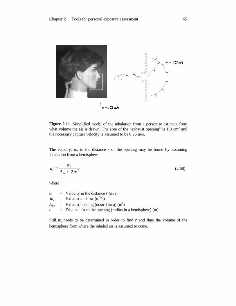
Chapter 2 Tools for personal exposure assessment 65
Figure 2.11. Simplified model of the inhalation from a person to estimate fromwhat volume the air is drawn. The area of the “exhaust opening” is 1.3 cm2 andthe necessary capture velocity is assumed to be 0.25 m/s.
The velocity, ur, in the distance r of the opening may be found by assuminginhalation from a hemisphere
um
A rrr
Ex
=+�
2 2π(2.68)
where
ur = Velocity in the distance r (m/s)�mr = Exhaust air flow (m3/s)
AEx = Exhaust opening (nostril area) (m2)r = Distance from the opening (radius in a hemisphere) (m)
Still, �mr needs to be determined in order to find r and thus the volume of the
hemisphere from where the inhaled air is assumed to come.

Henrik Brohus66
According to Table 2.5. the pulmonary ventilation for a person at moderate workis 30 l/min. The inhalation, however, does not take place continuously butapproximately 12 times per minute, intermittently. If the inhalation takes placehalf the time, �mr = 60 l/min is obtained. For ur = 0.25 m/s and AEx = 1.3 cm2, r =
2.5 cm. This corresponds to a hemisphere volume of approximately 30 cm3.
For an activity level corresponding to rest r = 1 cm, and the hemisphere volume isapproximately 2 cm3, i.e. in both cases relatively small volumes and smalldistances from the nose/mouth are obtained.
The above analysis suggests that the personal exposure for the CSP´s may besimulated as the mean concentration of a volume between 2 cm3 and 30 cm3
adjacent to the surface in breathing zone height, i.e. 1.5 m above the floor for astanding average sized woman and for the BTM.
In the CFD simulations two different concentrations regarding the personalexposure have been determined, namely the concentration in the cell closest to thebreathing zone (~ 10 cm3) and the mean concentration of a volume around thebreathing zone including more cells (~ 30 cm3).
Comparing the two concentrations reveals a relatively strong dependence on theconcentration gradient close to the breathing zone, the higher gradient the greateris the deviation between the two concentrations, as may be expected. Ratiosbetween the concentration in the “volume” and the nearest cell are found in therange of 0.5 to 5. This stresses the importance of the topic and the possibleinfluence on the personal exposure assessment. Most of the results, however,show approximately equal concentration levels.
In the following chapters the personal exposure calculated by means of CFDcorresponds to the contaminant concentration in the nearest cell along theComputer Simulated Person at a height of 1.5 m.

Chapter 2 Tools for personal exposure assessment 67
2.4. Trained Sensory Panel
2.4.1. Introduction
The aim of modelling the personal exposure is to assess what people actuallyinhale when they are located in a certain environment where contaminant sourcesprevail. Therefore, it seems obvious to use people as measuring instruments ifpossible and affordable.
People may be applied as an instrument in the determination of the contaminantconcentration in two different ways, directly and indirectly.
Indirectly, by wearing a passive or an active sampling device, i.e. personalmonitors located close to the breathing zone. Continuously or integrated thisdevice may collect different kinds of gasses, particles, etc. In order to interpret theresults it is necessary to know the relationship between the concentrationmeasured by the sampler and what is actually inhaled. This is usually assumed tobe the same, even though some investigations have reported deviations (e.g.Martinelli et al., 1983; Rodes et al., 1991; 1995). As mentioned in Chapter 1 thedeviations depend on the concentration gradients in the breathing zone, amongother things, which will be discussed in greater detail in the subsequent chapters.
Directly, personal exposure may be determined by locating a sampling deviceinside or very close to the mouth or the nose, for instance in shape of a tubeconnected to a pump and a gas analyser. This approach has been applied byMundt (1994).
Another method is biological monitoring where biological markers are used toindicate exposure. The markers may be blood, urine, sputum or exhaled air(Sexton and Ryan, 1988). For instance, exhaled air was filled on a bottle andanalysed to assess the personal exposure by Pleil and Lindstrom (1995).However, some difficulties arise when biological monitoring is used due to thefact that it is the dose rather than the exposure that is determined, andassumptions regarding respiration frequency, depth of inspiration, etc. may benecessary in order to assess the personal exposure where this approach is used.
A third way of determining personal exposure is by means of a Trained SensoryPanel (TSP). This is especially convenient when transient phenomena are studied

Henrik Brohus68
which occur when people are entering a room causing disturbances while they areinhaling room air and judging the air quality (Brohus et al., 1996).
A TSP is applied in this work to assess the personal exposure and the perceivedair quality. The topic is further discussed in the following, including theassessment of perceived air quality and definitions of the sensory units olf anddecipol.
2.4.2. Assessment of perceived air quality
Humans perceive the air as a combined response of the olfactory sense and thegeneral chemical sense. The olfactory sense is situated in the nasal cavity and issensitive to several hundred thousand odorants in the air. The general chemicalsense is located all over the mucous membranes in the eyes and in the nose, and itis sensitive to a similarly large number of irritants in the air (ECA, 1992). Thesesenses determine whether the air feels fresh and pleasant or stale and stuffy,whether the air irritates or not, and whether the air can be judged acceptable orunacceptable.
Perceived air quality is defined as the immediate impression of the indoor airquality experienced by the people entering a space (Fanger, 1988). Perceived airquality can also be expressed as the percentage of dissatisfied, PD, i.e. thosepersons who perceive the air to be unacceptable just after entering the space.
Sensory units
In order to quantify air pollution and air pollution sources as perceived byhumans Fanger (1988) defined the two sensory units, the olf and the decipol.
One olf is the emission rate of air pollution (bioeffluents) from a standard person(sedentary activity level of 1 met , average skin area of 1.8 m2, hygienic standardof 0.7 bath/day and changing underwear every day). Other pollution sources arethen expressed as person equivalents, i.e. the number of standard persons (olfs)required to make the air as annoying, thus causing the same dissatisfaction, as theactual pollution source.

Chapter 2 Tools for personal exposure assessment 69
When more sensory pollution sources are present at the same time the totalsensory pollution load can as a first approximation be determined by simpleaddition of the sensory load of the single sources (Bluyssen and Fanger, 1991;Wargocki et al., 1996).
Bluyssen and Fanger (1991), however, emphasise that further research may showthat air qualities caused by mixtures of some materials may be perceived strongeror weaker than predicted by simple addition. Knudsen et al. (1994) found that thesensory emission rates for three frequently used materials vary with the pollutionconcentration, but they also found that the mixture of the three materials causes apercentage of dissatisfied approximately equal to the average of the individualmaterials.
Figure 2.12. shows the percentage of dissatisfied, PD, as a function of theventilation rate per olf (standard person).
Figure 2.12. Dissatisfaction caused by one standard person (one olf) whenventilated by unpolluted outdoor air at different ventilation rates, q. Based onequations (2.69) and (2.70) by Fanger (1988).
( )PD q= ⋅ −395 138 0.25exp . for q ≥ 0.32 l/s⋅olf (2.69)
PD = 100% for q < 0.32 l/s⋅olf (2.70)
0
25
50
75
100
0 5 10 15 20
Ventilation rate (l/s olf)
PD
(%
)
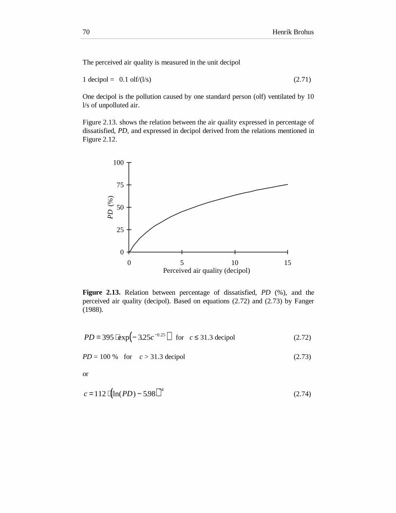
Henrik Brohus70
The perceived air quality is measured in the unit decipol
1 decipol = 0.1 olf/(l/s) (2.71)
One decipol is the pollution caused by one standard person (olf) ventilated by 10l/s of unpolluted air.
Figure 2.13. shows the relation between the air quality expressed in percentage ofdissatisfied, PD, and expressed in decipol derived from the relations mentioned inFigure 2.12.
Figure 2.13. Relation between percentage of dissatisfied, PD (%), and theperceived air quality (decipol). Based on equations (2.72) and (2.73) by Fanger(1988).
( )PD c= ⋅ − −395 325 0 25exp . . for c ≤ 31.3 decipol (2.72)
PD = 100 % for c > 31.3 decipol (2.73)
or
( )c PD= ⋅ −−
112 5984
ln( ) . (2.74)
0
25
50
75
100
0 5 10 15Perceived air quality (decipol)
PD
(%
)

Chapter 2 Tools for personal exposure assessment 71
If it is assumed that the sensory sources are additive the total effect may beexpressed, taking the ventilation effectiveness into account, as
c cq
GG G G
e outout
eqe e
n
e n
= + + + + +
−10 21
1
2
2ε ε ε, , ,
� (2.75)
where
ce = Personal exposure or perceived air quality (decipol)cout = Perceived air quality of outdoor air (decipol)qout = Ventilation rate of unpolluted outdoor air (m3/s)Geq = Source strength of ventilation equipment (olf)Gn = Pollution source strength regarding source no. n (olf)εe,n = Personal exposure index regarding source no. n (n.d.)
The addition of sensory sources should not be confused with the addition ofsensory effects on people. Percentage of dissatisfied, intensity of odour or sensoryirritation are not proportional to the concentration, consequently, they are notadditive (Wargocki et al., 1996).
Sensory panel
In order to determine the perceived air quality a sensory panel is used. The panelmay be untrained (naïve) or trained.
An untrained panel comprises a group of persons unrelated to the space to beexamined. The panel members are asked to judge whether the air quality isacceptable or not, imaging s/he be exposed to such air quality every day. Thus thepercentage of dissatisfied provides the perceived air quality (ECA, 1992). Thenecessary number of panel members depends on the required statistical confidencebut it will typically be in the range of 20 - 50 people (Pejtersen and Mayer, 1993).
In this work a Trained Sensory Panel (TSP) is applied. A TSP comprises a groupof persons trained to judge the air quality in comparison with references withknown levels of perceived air quality. A panel of minimum six persons isrecommended (ECA, 1992). Here, a panel of 14 persons (eleven male and threefemale) is selected from a larger group of naïve subjects on the basis of anentrance test.

Henrik Brohus72
The panel is trained to assess the air quality directly in the sensory unit decipol incomparison with five 2-propanone references ranging from 1 to 20 decipol, seeFigure 2.14.
Figure 2.14. Five known 2-propanone references (milestones) of 1, 3, 5, 10 and20 decipol used by the Trained Sensory Panel for judging the perceived airquality. The references consist of a 3-litre glass jar with a ventilated diffuser (~0.9 l/s). Inside the jar the 2-propanone is generated by passive evaporation frompure liquid 2-propanone in 30 ml bottles. According to Bluyssen and Fanger(1991) the references can be calibrated using the relation: decipol = 0.84 +0.22⋅ppm.
During the training the panel members are exposed to unknown 2-propranoneconcentrations which should be compared with the known references in order todetermine the perceived air quality.

Chapter 2 Tools for personal exposure assessment 73
The subjects are allowed to go back and forth between the unknown and theknown concentrations as many times they require, but they should always take atleast two inhalations of fresh air between each judgement to avoid adaptation.After the voting they are told the correct answer.
The training of the panel is started with a larger initial training period and thenfollowed by approximately half an hour of training before each experimentalsession, corresponding to two unknown 2-propanone concentrations.
In order to evaluate the performance of the panel and to be able to calibrate theTSP, 8 different 2-propanone concentrations unknown to the panel are judged byevery member on every experimental session without any feedback. It is thusassumed that if a panel member has judged the 8 2-propanone concentrationssatisfying s/he will also be able to perform satisfying during the actualexperiment.
It has been observed (e.g. Pejtersen and Mayer, 1993; Knudsen et al., 1994) thatsome subjects may have a systematic error when assessing the 2-propanoneconcentrations. The subjects tend to vote too high on concentrations below fivedecipol and too low on concentrations above five decipol. To eliminate thissystematic error, the relation between voted and expected perceived air quality ismodelled by means of a power function (Pejtersen and Mayer, 1993)

Henrik Brohus74
Figure 2.15. Members of a Trained Sensory Panel assessing the air quality incomparison with five levels of a known reference.
Voted perceived air quality = A ⋅ (Expected perceived air quality)B (2.76)
The coefficients A and B are estimated by non-linear least-squares regression. Aand B are determined for every single subject on account of all assessments duringthe entire experimental period according to the recommendations of Knudsen(1994). The specific coefficients for the single subjects are then used to calibratethe assessments by
Calibrated perceived air quality = (1/A voted perceived air quality)1/B (2.77)
2.4.3. Personal exposure assessment using the TSP
A TSP can be used in personal exposure assessment in different ways. It can ofcause be applied in the assessment of perceived air quality. This may de done

Chapter 2 Tools for personal exposure assessment 75
both in full scale, and also in small-scale using a diffuser like the ones shown inFigure 2.15. (Knudsen et al., 1993). Assumptions regarding full scale versussmall scale air flow pattern and contaminant distribution have to be made, forinstance, it can be necessary to apply fully mixed conditions in small scale andthen translate the results to full scale by using the personal exposure index, εe, orby other means (Jensen and Nielsen, 1995).
The TSP may also be used to determine the concentration of a certain referencegas in comparison with “milestones” of known levels, for instance the 2-propanone. In case of 2-propanone the level assessed in the decipol unit mayeasily be converted to the ppm unit using the following relation (Bluyssen andFanger, 1991)
c cdp ppm= + ⋅084 0 22. . (2.78)
where
cdp = Perceived air quality using 2-propanone as reference (decipol)cppm = Concentration of 2-propanone (ppm)
In this way it is possible to use 2-propanone as a tracer gas that may simulate thebehaviour of contaminant sources in a ventilated room etc. The perceived airquality assessed by the sensory panel, cdp, may then be converted into the personalexposure, ce, which in this case equals cppm. One great advantage of this approachis the fact that it is also possible to measure the concentration of the reference gaschemically. Consequently, in the case of a ventilated room where 2-propanone isused as tracer gas the exhaust concentration, cR, may be determined chemicallyand the personal exposure may be assessed by real persons and, finally, thepersonal exposure index, εe, can be determined. In that way it is possible toinclude the effect of transient behaviour of real people, which may be relevant,especially in assessment of short-term exposure and determination of theperceived air quality (Brohus et al., 1996).
A very important limitation of the approach is the adaptation. On account of theadaptation only the first impression of the air quality is valid, i.e. when a memberof the trained panel enters a polluted room only the first inhalation can be used inthe assessment. This method is limited to (very) short-term exposuremeasurements.

Henrik Brohus76

Chapter 3 Displacement ventilation 77
Chapter 3
Displacement ventilation
3.1. Introduction
The tools for personal exposure assessment described in Chapter 2 will now beapplied on the two major room ventilation principles, the displacement principleand the mixing principle in Chapter 3 and Chapter 4, respectively.
This will be done in order to examine some of the characteristics regardingpersonal exposure for the two ventilation principles, and to develop knowledgeand models that may facilitate the assessment. This will also highlight thedeviations between the actual exposure and the assessment by means of the widelyused compartmental approach, where the room air is assumed to be completelymixed.
Chapter 3 and Chapter 4 may serve as an illustration on the usage of the toolsintroduced in Chapter 2, i.e. the Breathing Thermal Manikin, the ComputerSimulated Person, and the Trained Sensory Panel. The tools will be discussed andevaluated by means of comparisons with each other together with results from theliterature.
The present Chapter 3 will start by summarising the characteristics ofdisplacement ventilation. Then full-scale measurements and CFD simulations onpersonal exposure will be presented including the proposal of a simple exposuremodel that may be applied in the practical design of displacement ventilationsystems. To generate the contamination warm and cold point contaminant sourcesare applied together with a planar source in the shape of the floor in thedisplacement ventilated room.

Henrik Brohus78
3.2. Characteristics of displacement ventilation
In the following some of the important characteristics of displacement ventilationwill be mentioned and discussed in order to give an overview of the ventilationprinciple, and to clarify some concepts and ideas applied in the presentedmeasurements and simulations presented.
According to Mundt (1996) displacement ventilation has been used in buildings toextract excess heat and contaminants since the antique and the middle age. Fromthe 1950s displacement ventilation experienced a renaissance in industrialapplications, and from the 1980s the principle became popular in comfortventilation, especially in the Scandinavian countries.
The reason for the growing interest in the displacement principle is a possibility ofobtaining a relatively high ventilation effectiveness and temperature effectiveness,and thus the possibility both to supply fresh air to the occupants and to removecontaminants and excess heat in an energy efficient and cost effective way.However, there are some limitations that should be acknowledged in order toperform a proper choice of ventilation principle and a successful design of thesystem.
Thermally controlled ventilation
Using displacement ventilation subcooled air is supplied in the lower part of theoccupied zone of the ventilated room. The air is supplied with a low momentum(velocity) and a low turbulence level. Due to the gravity force affecting the denseair it spreads out radially along the entire floor in an almost horizontal layer withonly very limited entrainment of the surrounding room air.
If the room is large (long) the flow will gradually be dissolved and entrained intothe heat sources. If the room is small multiple reflections occur at the walls(Etheridge and Sandberg, 1996), see Figure 3.1. By repeated reflections the lowerpart of the room is filled with air, while part of the gravity current is entrainedinto the plumes of the heat sources or in the boundary layer flow along the wallswhich are often warmer than the surrounding air in the lower part of a typicaldisplacement ventilated room.

Chapter 3 Displacement ventilation 79
Figure 3.1. Air distribution in a typical displacement ventilated room. Thesubcooled air is supplied in the occupied zone (1), it spreads radially along thefloor (2), it is reflected at the walls (3), and part of the current is entrained intoheat sources (4) and warm walls (5). In the upper part of the room a recirculationzone is generated (6), and the air is extracted through exhaust openings locatedclose to the ceiling (7).
In that way a stratified flow is obtained which is almost unidirectional in thelower part of the room. This kind of flow is thermally controlled and it isgoverned by the buoyancy forces in the fluid (e.g. expressed by the Archimedesnumber, Ar).
Even though the “old” air is displaced upwards, it must not be confused withpiston flow (or plug flow) where the flow is controlled mainly by inertial forces(i.e. Ar ~ 0). Displacement ventilation is significantly influenced by the internalheat sources of the room and it is therefore also called source ventilation,especially in German literature (Fitzner, 1996).
The heat from the internal heat sources raises to the ceiling which in this way isheated together with the upper part of the room. Part of this heat is redistributedto the floor and the lower part of the room by means of radiative heat transfer. Itresults in a temperature distribution with a significantly vertical gradient. Thistemperature gradient facilitates removal of exhaust air at ceiling level severaldegrees above the temperature in the occupied zone. This allows an efficient useof energy, but it may also give rise to thermal discomfort if the temperature

Henrik Brohus80
differences are too large. Therefore, the vertical temperature gradient is animportant design parameter to consider (Nielsen, 1993).
Stratification
The flow is unidirectional until the height where the net air flow rate of plumesgenerated by the heat sources equals the supply air flow rate. Above this height,i.e. the stratification height yst, a recirculation zone is generated.
If the contaminant sources also are heat sources the displacement ventilationsystem can have a high ventilation effectiveness. In this case the stratified flowimplies that the room is separated in a lower, cleaner part and an upper, morecontaminated part. The two zones are separated at the stratification height, yst, byan interfacial layer with a typical thickness of approximately 0.5 m (Etheridgeand Sandberg, 1996), see Figure 3.2.
The concentration distribution is one of the important differences betweendisplacement ventilation and conventional mixing ventilation regarding the airquality. In displacement ventilated rooms the air quality in the occupied zone iscomparable with the supply air quality, while in mixing ventilation it iscomparable with the exhaust air quality.
If the convection current from the contaminant source, in a room with several heatsources, is not the warmest, the contaminant may settle in a layer where theconcentration locally exceeds the exhaust concentration (Skistad, 1994), seeFigure 3.2. This phenomenon may influence the air quality, especially if a certainconcentration peak is located in the lower part of the occupied zone.
It is found that the stratification of the flow is quite stable, even if people aremoving around in a displacement ventilated room. Especially the thermalstratification is stable (also in case of relatively violent movements in theventilated room), while the concentration distribution is slightly more affected, buteven if the room air is temporarily mixed, the stratification is quickly re-established (Brohus and Nielsen, 1994a).
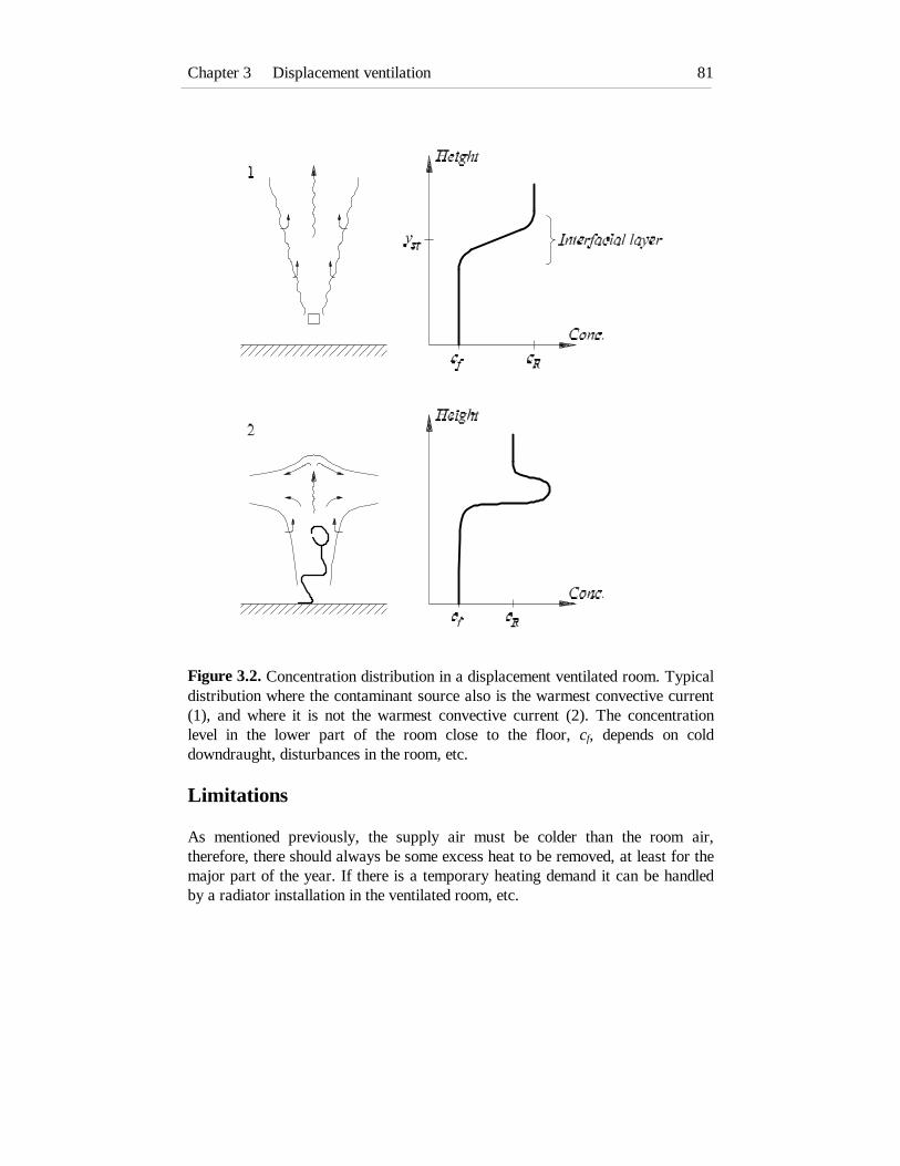
Chapter 3 Displacement ventilation 81
Figure 3.2. Concentration distribution in a displacement ventilated room. Typicaldistribution where the contaminant source also is the warmest convective current(1), and where it is not the warmest convective current (2). The concentrationlevel in the lower part of the room close to the floor, cf, depends on colddowndraught, disturbances in the room, etc.
Limitations
As mentioned previously, the supply air must be colder than the room air,therefore, there should always be some excess heat to be removed, at least for themajor part of the year. If there is a temporary heating demand it can be handledby a radiator installation in the ventilated room, etc.

Henrik Brohus82
The contaminant sources should also be heat sources or lighter than the ambientair to obtain the concentration stratification. At the same time the exhaust openingmust be located close to the ceiling.
In order to avoid thermal discomfort it is important to be aware of the adjacentzone close to the inlet device where the velocity is high and the temperature islow, as well as the vertical room air temperature gradient.
Personal exposure considerations
When dealing with personal exposure, displacement ventilation seems to be anobvious way to obtain a very high personal exposure index, εe, in the case ofwarm contaminant sources and a stratification height located above the breathingzone.
However, what happens when the stratification height is located below thebreathing zone height? This is an important question due to the fact that thestratification height is determined primarily by the supply air flow rate in a givenset-up of heat and contaminant sources. Therefore, if it is possible to reduce thenecessary stratification height, the flow rate and consequently the energyconsumption will be reduced accordingly.
Another relevant question regarding personal exposure is the influence ofthermally passive contaminant sources, e.g. a point source located close to aperson or a planar source in the shape of the entire floor, etc.
Furthermore, how is the perceived air quality in a ventilated room affected whenthe displacement principle is applied? Here, the transient behaviour isconsiderable whereas most recommendations and measurements assume steady-state conditions.
The above-mentioned questions will, among other things, be examined by meansof the following measurements and simulations.

Chapter 3 Displacement ventilation 83
3.3. Measurements using a BTM
In this chapter personal exposure measurements comprising a Breathing ThermalManikin in a displacement ventilated room are presented. First, the experimentalset-up will be outlined, then the topic “exposure in proportion to the stratificationheight” will be examined and, finally, the effect of a passive point source will beinvestigated.
3.3.1. Experimental set-up
The personal exposure measurements presented in this chapter are performed bymeans of the Breathing Thermal Manikin (BTM) which is discussed in detail inChapter 2.2. The measurements are performed in the full-scale displacementventilated room shown in Figure 3.3. and Figure 3.4.
The room in Figure 3.3. consists of an outer steel framework to which the floor,ceiling and the walls are attached. Two of the walls consist of double glazedwindows in order to facilitate smoke visualisation, the other walls are made of 20mm Douglas wood laminates. The floor and the ceiling are insulated with 10 mmpolystyrene and 50 mm glass wool, respectively. The entire test room is containedinside a conditioned laboratory building, see Figure 3.5.

Henrik Brohus84
Figure 3.3. Displacement ventilated full-scale test room. The subcooled air issupplied by a low-velocity inlet device (1) and it is exhausted through two returnopenings in the ceiling. The heat load is generated by two person simulators (2,3),a point heat source (4) and the Breathing Thermal Manikin (5), represented by abox in the figure.
In Figure 3.4. the displacement ventilated room is shown in a two-dimensionalplot where the locations of the different heat sources also are included.

Chapter 3 Displacement ventilation 85
Figure 3.4. Displacement ventilated full-scale test room. The subcooled air issupplied by a low-velocity inlet device (1) and it is exhausted through two returnopenings in the ceiling. The heat load is generated by two person simulators (2,3),a point heat source (4) and the Breathing Thermal Manikin (5), represented by abox in the figure.
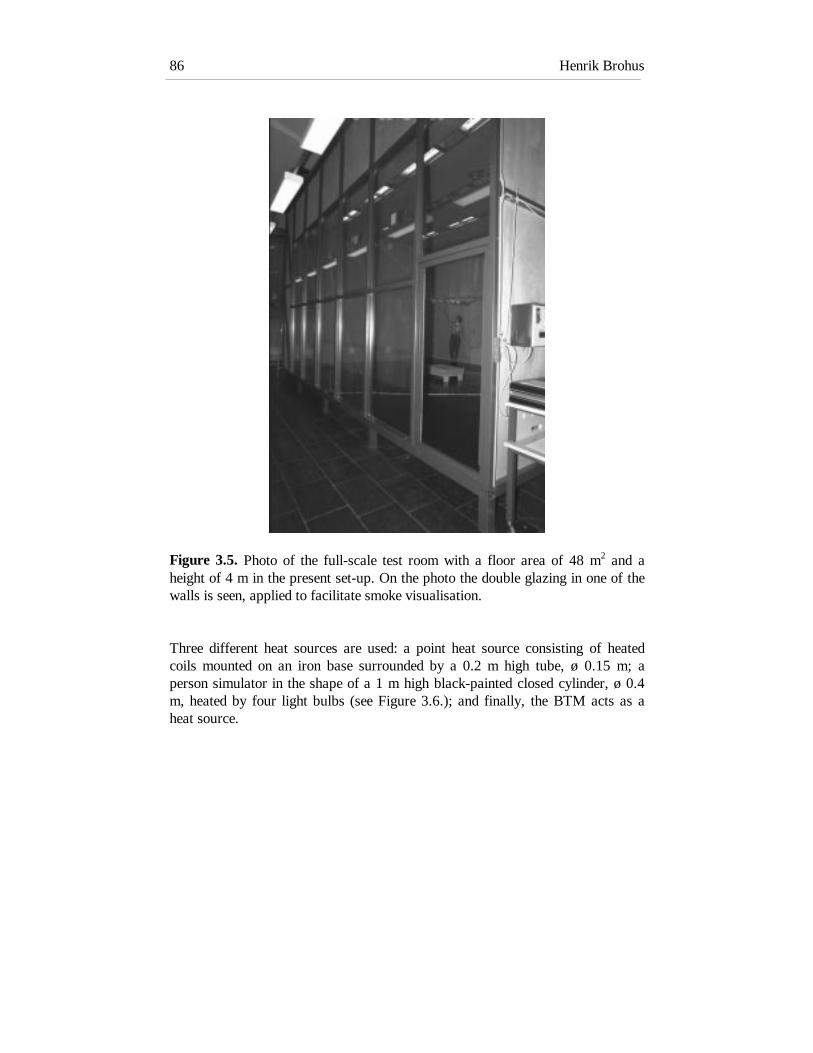
Henrik Brohus86
Figure 3.5. Photo of the full-scale test room with a floor area of 48 m2 and aheight of 4 m in the present set-up. On the photo the double glazing in one of thewalls is seen, applied to facilitate smoke visualisation.
Three different heat sources are used: a point heat source consisting of heatedcoils mounted on an iron base surrounded by a 0.2 m high tube, ø 0.15 m; aperson simulator in the shape of a 1 m high black-painted closed cylinder, ø 0.4m, heated by four light bulbs (see Figure 3.6.); and finally, the BTM acts as aheat source.

Chapter 3 Displacement ventilation 87
Figure 3.6. Photos of the point heat source (left) and the person simulator (right).The inlet device is seen in the upper right corner.
Two kinds of contaminant sources are examined, a passive source and a non-passive source. The non-passive source is simulated by nitrous oxide (N2O)injected through an upward pointing tube, ø 0.01 m. The tube is located above aheat source at an elevation of 2 m. The passive contaminant source is simulatedby a neutral density mixture of nitrous oxide and helium (He) injected through aporous foam rubber ball, ø 0.1 m, see Figure 3.7.
The tracer gas concentration is measured by photoacoustic spectroscopy(uncertainty ± 2%). The temperatures are measured by thermocouples, type k(uncertainty ± 0.2°C). The velocities are measured by temperature-compensatedhot sphere anemometers (uncertainty ± 0.02 m/s).

Henrik Brohus88
Figure 3.7. Photos of the two contaminant sources applied in the measurements.Both are used for tracer gas injection. Left: upward pointing tube, ø 0.01 m,located above a heat source (non-passive source). Right: porous foam rubber ball,ø 0.1 m (passive source). N2O is used as tracer gas in both cases, and for thepassive source it is mixed with He to obtain a neutral density mixture comparedwith the room air.
3.3.2. Exposure in proportion to stratification height
The measurements presented in Chapter 3.3.2. are made in collaboration withChristensen and Stevnhoved (1993). The steady-state exposure measurements arecarried out with respiration through the mouth. In the present measurements nosignificant differences between respiration through the mouth and respirationthrough the nose are found.
Three different cases are examined corresponding to different stratificationheights. In Table 3.1. the key parameters are summarised, and in Figure 3.8. andFigure 3.9. the vertical temperature distribution and the velocity profile areshown, respectively.

Chapter 3 Displacement ventilation 89
Table 3.1. Specification of the three cases examined in the full-scalemeasurements. q is the supply air flow rate, n is the air change rate, Φ is the heatload, t0 is the supply air temperature, tR is the return air temperature and yst is thestratification height (found by means of the measurements).
Case Parametersq
(m3/h)n
(h-1)Φ
(W)t0
(°C)tR
(°C)yst
(m)A 145 0.8 771 14.7 24.4 1.00B 290 1.5 376 17.6 22.6 1.35C 395 2.1 781 15.8 23.4 2.25
Figure 3.8. Dimensionless vertical temperature distribution in the displacementventilated room in Case A, B and C. The measurements are performed at (x,y) =(4,-1), i.e. 1 m beside the BTM, see Figure 3.4. The temperatures are madedimensionless by subtracting the supply air temperature and dividing by thedifference between the return and the supply air temperature, i.e. t* = (t - t0)/(tR -t0).
0
1
2
3
4
0.0 0.5 1.0
Temperature (n.d.)
Hei
ght (
m)
Case A
Case B
Case C
tt t
t tR
* =−−
0
0

Henrik Brohus90
The temperature profiles seen in Figure 3.8. are typical for a displacementventilated room, both regarding the surface temperatures and the vertical airtemperature distribution. The outline of the curves with a relatively high gradientin the lower part of the room and a smaller (or almost no) vertical gradient in theupper part is also quite typical, even though differences may occur depending onthe type and the intensity of the heat sources, among other things, (Nielsen, 1996;Mundt, 1996).
Figure 3.9. Vertical velocity profiles in the displacement ventilated room in CaseA, B and C. The measurements are performed at (x,z) = (4,0) which correspondsto the location of the BTM. During the velocity measurements, the manikin istemporarily moved, for which reason the velocities represent the undisturbedvelocity field at the location of the BTM.
Like the temperature distribution the velocity profiles are typical for adisplacement ventilated room with high velocities close to the floor, and above theprimary flow a secondary return flow in the opposite direction with a significantlylower level.
Both the temperature and the velocity levels correspond well to thermal comfortconditions for a typical activity level in usual indoor environments.
0
1
2
-0.1 0.0 0.1 0.2 0.3
Velocity (m/s)
Hei
ght (
m) Case A
Case B
Case C

Chapter 3 Displacement ventilation 91
Figure 3.10. Dimensionless exposure (∗∗∗∗) and vertical concentration distribution(Ο) measured for the three stratification heights 1.00 m (Case A), 1.35 m (CaseB) and 2.25 m (Case C) for the seated (left) and standing (right) BTM. Themeasurements are performed at (x,z) = (3,-1). The exposure is measured at ye =1.1 m for the seated manikin and at ye = 1.5 m for the standing manikin. In CaseA and B the tracer gas is supplied above the heat source (3) in Figure 3.3. In CaseC the tracer gas is supplied above the heat source (4) in Figure 3.3.
Case A - Seated
0
1
2
3
4
0.0 0.5 1.0 1.5Concentration (n.d.)
Hei
ght (
m)
Case A - Standing
0
1
2
3
4
0.0 0.5 1.0 1.5Concentration (n.d.)
Hei
ght (
m)
Case B - Seated
0
1
2
3
4
0.0 0.5 1.0 1.5Concentration (n.d.)
Hei
ght (
m)
Case B - Standing
0
1
2
3
4
0.0 0.5 1.0 1.5Concentration (n.d.)
Hei
ght (
m)
Case C - Standing
0
1
2
3
4
0.0 0.5 1.0 1.5Concentration (n.d.)
Hei
ght (
m)
Case C - Seated
0
1
2
3
4
0.0 0.5 1.0 1.5Concentration (n.d.)
Hei
ght (
m)

Henrik Brohus92
Table 3.2. Results from personal exposure measurements in a displacementventilated room using a Breathing Thermal Manikin. ce
* is the dimensionlesspersonal exposure, εoc is the ventilation effectiveness in the occupied zone, and εe
is the personal exposure index. The results correspond to the concentrationdistributions shown in Figure 3.10. and the specifications in Table 3.1.
Case BTMposition
ce*
(n.d.)εoc
(n.d.)εe
(n.d.)A Seated
Standing0.470.57
1.441.54
2.131.75
B SeatedStanding
0.280.50
1.651.84
3.572.00
C SeatedStanding
0.060.06
12.4112.08
16.6716.67
In Figure 3.10. the exposure of a seated and a standing person in the shape of theBTM is shown at the three stratification heights, yst, 1.00 m, 1.35 m and 2.25 m.The dimensionless exposure, ce
*, the ventilation effectiveness in the occupiedzone, εoc, and the personal exposure index, εe, for the three cases are summarisedin Table 3.2. In all three cases the manikin (approximately 75 W), the two personsimulators (2 x 100 W), and the point heat source (100 W or 500 W) constitutethe heat load in the room.
Due to the uninsulated walls there is a slight heat transfer between the room andthe surrounding laboratory. The difference between the mean room airtemperature and the mean surface temperature is less than 0.5°C. Nevertheless,due to the temperature gradient there will be a heat gain in the lower part and aheat loss in the upper part. At the walls this causes a slight upward convectiveflow at the lower surfaces and a slight downward convective flow at the uppersurfaces. The net effect is presumably of no significant importance in this context,a conclusion that is confirmed also by smoke tests.
One effect, however, that is clearly seen on the concentration profiles is therelatively high concentration in the lower part of the room, which is considerablyhigher than zero. This may have been caused by transport of contaminant fromthe upper part of the room to the lower part by downward convection currents insome parts of the room. This phenomenon may easily be found in practice too,e.g. in case of cold downdraught from windows, etc. Therefore, it is relevant totake this into account when the personal exposure is assessed, which is possibleby using the present measurements.

Chapter 3 Displacement ventilation 93
As seen in Figure 3.10. the effect of entrainment and transport of room air fromthe lower and cleaner zone to the breathing zone is distinct, which is also pointedout by Holmberg et al. (1990), Stymne et al. (1991) and Etheridge and Sandberg(1996) among others. This means that the concentration of inhaled contaminant issmaller than the corresponding concentration at the same height at a “neutral”place in the room. In this case the entrainment provides a better indoor air qualityin the displacement ventilated room than in a room with mixing ventilation.
The figure shows also that the ventilation effectiveness in the occupied zone ishigher than in the case of mixing ventilation, where εoc approaches 1 in the idealcase. As expected, the effectiveness increases with increasing stratification height.In all cases the personal exposure index, εe, exceeds εoc, indicating that the qualityof the inhaled air exceeds the mean indoor air quality in the occupied zone.
3.3.3. Personal exposure model for a displacementventilated room
The exposure depends, among other things, on the concentration in the lower zoneof the room. At the same stratification height this concentration may vary fromcase to case depending on the inlet device, the air temperature differences, the heatand contaminant source configuration, room surface temperatures, etc. To be ableto take the concentration in the lower zone into account a new quantity is defined:the effectiveness of entrainment in the human boundary layer, designated ηe
ηeP e
P f
c c
c c=
−−
(3.1)
where cf is the concentration at the floor that typically corresponds to theconcentration in the lower, cleaner zone of the displacement ventilated room, seeFigure 3.11.

Henrik Brohus94
Figure 3.11. Virtual concentration distribution in a displacement ventilated room.ye is the breathing zone height and yst is the stratification height. ce is located inbetween cP and cf due to the effect of entrainment in the human boundary layer.
The effectiveness of entrainment in the human boundary layer, ηe, expresses theability to supply (fresh) air from the floor area to the breathing zone. It expressesthe utilised fraction (cP - ce) of the possible concentration difference (cP - cf).
When ηe = 1, all the inhaled air comes from the lower zone and ce equals theconcentration at the floor, cf. When ηe = 0 the exposure equals the concentrationcP at the breathing zone height, i.e. no particular effect because of the convectivetransport in the human boundary layer, see Figure 3.12.
Figure 3.12. Effectiveness of entrainment in the human boundary layer, ηe. Whenthe stratification height, yst, decreases, the effectiveness decreases. When thestratification increases to the breathing zone height, ye, the effectiveness ofentrainment in the human boundary layer approaches 1.

Chapter 3 Displacement ventilation 95
In the case of complete mixing as well as in displacement ventilation with astratification height located above the breathing zone, ηe is not defined. In thesecases ce equals the homogeneous concentration in the room or the concentration inthe lower zone, respectively. This implies that ηe ≡ 1 for cP = cf.
One advantage of using ηe is the independence of the concentration in the lowerzone that may vary in different cases. This enables and improves the comparisonof results from different test rooms and different experimental set-ups.
From the results in Figure 3.10., ηe is calculated for Case A - Seated (0.91),Case A - Standing (0.66) and Case B - Standing (0.78), where the quantity isdefined. It illustrates the extent to which the inhaled air is supplied from the lowerand cleaner zone. In Case A - Seated, almost all air comes from the lower zone,while in Case A - Standing, only somewhat more than half of the air arises fromthe lower zone. The reason why ηe is lower in the Case A - Standing is the factthat the breathing zone is located at a higher level. This implies that morecontaminated air is entrained in the boundary layer before it reaches the breathingzone where it is inhaled.
If ce is expressed by means of the new quantity, we get the following equation
( )c c c ce P e P f= − −η (3.2)
i.e. the concentration of inhaled contaminant is expressed as a function of theconcentration at the breathing zone height unaffected by a present person (cP), theconcentration at the floor, and the effectiveness of entrainment in the humanboundary layer. If ηe is known, equation (3.2) can be used to estimate thepersonal exposure in a displacement ventilated room.
In the expression for ηe, the stratification height must be considered due to thesignificant influence of this parameter. If we furthermore want to incorporate theheight of the breathing zone, ye, the dimensionless height yst/ye may be used. Thisquantity attains the value from 0 to 1 when the stratification height increases fromthe floor to the breathing zone height, which is the range of interest in this context.Consequently, if the effectiveness of entrainment in the human boundary layer isexpressed as a function of yst/ye, we may expect that ηe ranges from 0 to 1 whenyst/ye increases from 0 to 1 (see Figure 3.12.).
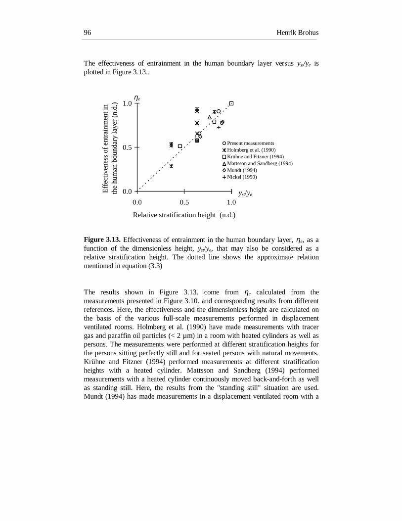
Henrik Brohus96
The effectiveness of entrainment in the human boundary layer versus yst/ye isplotted in Figure 3.13..
Figure 3.13. Effectiveness of entrainment in the human boundary layer, ηe, as afunction of the dimensionless height, yst/ye, that may also be considered as arelative stratification height. The dotted line shows the approximate relationmentioned in equation (3.3)
The results shown in Figure 3.13. come from ηe calculated from themeasurements presented in Figure 3.10. and corresponding results from differentreferences. Here, the effectiveness and the dimensionless height are calculated onthe basis of the various full-scale measurements performed in displacementventilated rooms. Holmberg et al. (1990) have made measurements with tracergas and paraffin oil particles (< 2 µm) in a room with heated cylinders as well aspersons. The measurements were performed at different stratification heights forthe persons sitting perfectly still and for seated persons with natural movements.Krühne and Fitzner (1994) performed measurements at different stratificationheights with a heated cylinder. Mattsson and Sandberg (1994) performedmeasurements with a heated cylinder continuously moved back-and-forth as wellas standing still. Here, the results from the "standing still" situation are used.Mundt (1994) has made measurements in a displacement ventilated room with a
0.0
0.5
1.0
0.0 0.5 1.0
Relative stratification height (n.d.)
Effe
ctiv
enes
s of
ent
rain
men
t in
the
hum
an b
ound
ary
laye
r (n
.d.)
Present measurementsHolmberg et al. (1990)Krühne and Fitzner (1994)Mattsson and Sandberg (1994)Mundt (1994)Nickel (1990)
ηe
yst/ye

Chapter 3 Displacement ventilation 97
person sitting and a person walking around, respectively. Nickel (1990)performed measurements with a heated cylinder.
Although different "models" of a person are used in different experimental set-ups, the quantity ηe and the relation yst/ye seem to establish a way of expressingthe various results more generally.
If we make a linear equation fit on the plot in Figure 3.13. to obtain thecoefficients of the equation ηe = A + B(yst/ye), we find that A = 0.22 and B = 0.73with a coefficient of determination R2 = 0.58. This reveals that A is close to zeroand that B is close to one. With a power equation fit, the following relation ηe =C(yst/ye)
D is obtained. Here the coefficients C = 0.95 and D = 0.75 are found withR2 = 0.62.
These results suggest an almost linear relationship between ηe and yst/ye with astarting point close to origo and with the effectiveness of entrainment in thehuman boundary layer approaching 1 when the relative height approaches 1.
For practical engineering purposes and without considerable loss of accuracy, onemay use the simple relation
ηest
e
y
y= (3.3)
By inserting the above expression in equation (3.2) we obtain a model for thepersonal exposure in a displacement ventilated room.
This exposure model may also be obtained in another way by means of a zonalmodel approach. If it is assumed that the concentration of inhaled contaminant isa mixture of the concentration in the lower, cleaner part of the displacementventilated room and the upper, more contaminated part, we may get the followingexpression if the two parts of the room are assumed to contribute with an amountproportional to the height occupied by the person, i.e.
( )c
y c y y c
ye
st f e st P
e
=+ −
(3.4)

Henrik Brohus98
Hence,
( )c cy
yc ce P
st
eP f= −
− (3.5)
Comparing equations (3.2) and (3.5) reveals that ηe is expressed as yst/ye which infact is the approximate relation (3.3) found empirically from Figure 3.13.
Further analysis of the human boundary layer may show a non-linear dependenceof ηe on yst/ye and relations where more parameters are considered may be found,but still the above expression may serve as a reasonable approximation forpractical engineering use in the case of an exposed subject in a displacementventilated room.
One limitation of the model is the effect of persons' movements. Since the basicresults arise mainly from cases where a "still" model of a person is used, theequation (3.5) is not valid when the person is making violent movements or whenthe person is walking fast through the ventilated room. This topic is discussed ingreater detail below.
Another limitation may be the influence of an obstacle in front of the person. Ifthe boundary layer is disturbed or partially destroyed, the effect of entrainmentand transport is obviously reduced.
If, for instance, a person is sitting (or standing) very close to the edge of a table,the thermal boundary layer is locally interrupted and the convective transport ofair from below the table is significantly limited. The effect of this limitationdepends to a great extent on the horizontal distance between the person and theobstacle. If the distance between the table and the person exceeds the boundarylayer thickness, there will presumably be no reduction in the entrainment andtransport in the human boundary layer. According to Homma and Yakiyama(1988), the thickness of the thermal boundary layer in front of the chest of astanding person is 0.07 - 0.15 m. Although the boundary layer thickness in aseated position is greater, the order of magnitude suggests that even relativelysmall gaps between the person and the table will enable convective mass transferto take place.

Chapter 3 Displacement ventilation 99
When the two-zonal approach is applied together with the above personalexposure model it is possible to find theoretical expressions for the differentventilation effectiveness in a displacement ventilated room, when the stratificationheight, yst, the return concentration, cR, and the concentration in the lower part ofthe room, cf, are known.
Table 3.3. Expressions of the different ventilation effectiveness as a function ofthe stratification height, yst, etc. ε is the mean ventilation effectiveness, εoc is theventilation effectiveness in the occupied zone, εP is the local ventilation index, andεe is the personal exposure index. cR is the return concentration, and cf is theconcentration in the lower part of the room, yoc is the height of the occupied zone,usually up to 1.8 m, and H is the room height.
Ventilationeffectiveness
Definition Location relative tostratification height
Expression in case ofdisplacement ventilation
ε c cR / -
( )H
H y c cst f R+ −/ 1
εocc cR oc/ yoc ≤ yst c cR f/
yoc > yst
( )y
y y c c
oc
oc st f R+ −/ 1
εPc cR P/ yP ≤ yst c cR f/
yP > yst c cR R/ (= 1)
εec cR e/ ye ≤ yst c cR f/
ye > yst
( )y
y y c c
e
e st f R+ −/ 1
As seen from Table 3.3. all effectiveness apart from ε behaves in two differentways depending on the location relative to the stratification height.
In Figure 3.14. a plot of εe and εoc versus stratification height is seen in case of adisplacement ventilated room where cf = 0.3 cR.

Henrik Brohus100
Figure 3.14. Ventilation effectiveness in the occupied zone (yoc = 1.8 m), εoc, andpersonal exposure index, εe, for a standing person (ye = 1.5 m) and a seatedperson (ye = 1.1 m). cf/cR = 0.3, i.e. the concentration in the lower, cleaner part ofthe room amounts to 30% of the concentration in the upper, more contaminatedpart. The curves are based on the formulas shown in Table 3.3.
Figure 3.14. clearly shows the theoretical growth of effectiveness for increasingstratification height. It is found that εe (seated) ≥ εe (standing) ≥ εoc, ranging from1.00 to 3.33, where ye and yoc are both exceeded by the stratification height. If yst
is further increased εe and εoc remain constant as indicated in the figure.
The shape of the curves depends on the ratio between the concentration levels inthe lower part and the upper part of the room, cf/cR. In theory and in laboratorymeasurements cf may equal zero, but in practice the concentration in the lowerpart of the room may easily deviate from zero due to cold downdraught,movements in the room, use of cooled ceilings, etc. Figure 3.15. shows the effectof the ratio cf/cR on the personal exposure index, εe, for a standing person.
0
1
2
0 1 2 3 4
Effectiveness (n.d.)
Str
atifi
catio
n he
ight
(m
)εe (standing)
εe (seated)
εoc
cf/cR = 0.3
yst

Chapter 3 Displacement ventilation 101
Figure 3.15. Personal exposure index, εe, for a standing person (ye = 1.5 m) as afunction of the stratification height, yst, for different levels of the ratio between theconcentration in the lower and the upper part of a displacement ventilated room,cf/cR, ranging from 0% to 50%. The curves are based on the formula in Table 3.3.
Figure 3.15. shows the significance of the concentration level in the lower part ofthe room, and stresses that it is important to reduce the possible factors that mayfacilitate and increase mixing of the stratified air in this part of the room.
If the personal exposure model is used to design a displacement ventilation systemone has to know or to estimate cf. This may be done by means of measurements orcomputer simulations or by means of assumptions based on experience. Theassumptions may be based on knowledge of the geometry and the boundaries ofthe room together with the contaminant sources and the activities performed bythe occupants. cf will presumably be found in the range of 0 - 0.5 cR.
0
1
2
0 2 4 6Personal exposure index (n.d.)
Str
atifi
catio
n he
ight
(m
)
Standingperson
εe
yst 50% 30%
10%
40% 20%
0%

Henrik Brohus102
The effect of movements on personal exposure
The measurements shown in Figure 3.13. mainly represent cases where the modelof a person is sedentary or standing still. This fact raises the question as to theeffect of movement on personal exposure.
One extreme is a sedentary person or a person standing still. Here, equation (3.5)provides a reasonable model for personal exposure in a displacement ventilatedroom. The second extreme is the case of a person walking quickly through aventilated room. Here, the concentration of inhaled contaminant, ce, obviouslyapproaches the neutral concentration in the breathing zone height, cP, due to theconsiderable horizontal velocity generated around the breathing zone. This casecorresponds to ηe = 0. The actual case may be found somewhere between the twosituations, depending on several parameters, for example the type of work,activity level, etc.
This point is supported by measurements of Holmberg et al. (1990), where ηe
changed from 0.94 to 0.66 when the persons present changed from motionless tonatural motion in a seated position.
Measurements of Mattsson and Sandberg (1994) with a moving heated cylindermay serve as another illustration. From these measurements the effectiveness ηe iscalculated and shown in Figure 3.16. for three different velocities of the heatedcylinder continuously moved back-and-forth in a displacement ventilated room.Even though Figure 3.16. is an example involving only one heated cylinder in"systematic motions" at one stratification height, it clearly illustrates that theeffectiveness, ηe decreases when the movements increase as mentioned above.
Measurements and smoke tests with the Breathing Thermal Manikin located in awind channel confirm that the thermal boundary layer is considerably affected atuniform velocities above 0.05 - 0.10 m/s (Brohus and Nielsen, 1994b; Hyldgaard,1994).

Chapter 3 Displacement ventilation 103
Figure 3.16. ηe as a function of the velocity relative to a moving cylinder.Measurements from Mattsson and Sandberg (1994) with a heated cylindercontinuously moved back-and-forth in a displacement ventilated room.
Although the measurements, mentioned previously from Holmberg et al. (1990),show a decrease in ηe, there is still a significant effect of entrainment in thehuman boundary layer during "natural motion" in a seated position. This point issupported by Mundt (1994) who reports measurements where the concentration isfound close to the nose of a person walking around in a displacement ventilatedroom. Here, the exposure is significantly below the corresponding concentrationin the surroundings.
An improvement of the personal exposure model suggested above may beobtained by including the relative velocity, u, or the movements of the exposedperson, e.g.
ηest
e
fy
yu=
, (3.6)
0.0
0.5
1.0
0.0 0.1 0.2 0.3
Velocity (m/s)
Effe
ctiv
enes
s of
ent
rain
men
t in
the
hum
an b
ound
ary
laye
r (n
.d.) ηe
u

Henrik Brohus104
General model
The two-zonal approach, which is quite convenient in case of displacementventilation, may be expanded to a multi-zonal approach that may presumably beused in general. Here, the personal exposure, ce, may be thought of as acombination of a number of vertical concentrations along the height of the humanbody, e.g.
c w ce i ii
n
==∑
1
(3.7)
where
ce = Personal exposure (ppm)ci = Concentration at location i (ppm)wi = Weight function for location i (n.d.)
The weights wi may be based on geometry (height or area covered by ci) or it maybe more sophisticated and consider a number of significant parameters, forinstance
( )w f geometry activity u t Ari i i i= , , , , ... (3.8)
The simple model proposed in equation (3.5) may also be expressed in terms ofweights where the two concentrations are weighted according to their relativeheights, i.e.
c w c w ce f f P P= + (3.9)
where
wy
yf est
e
= =η and wy y
yP ee st
e
= − =−
1 η (3.10)
which is valid for ye ≥ yst.

Chapter 3 Displacement ventilation 105
3.3.4. Exposure in proportion to location of a passive pointcontaminant source
The above conclusions assume that the contaminant sources are also heat sources,generating the characteristic two-zone concentration distribution in thedisplacement ventilated room.
If the contaminant sources are passive, e.g. from building materials and other“cold” sources, the concentration distribution may be changed radically, and thusaffect the personal exposure.
A passive point contaminant source is defined as a pollutant source without anysignificant initial momentum or buoyancy, i.e. the pollution is supplied with avery low velocity at room air temperature and at room air density.
In Figure 3.17. the exposure of the standing BTM is found in the case of a "high"and a "low" location of a passive point contaminant source. Figure 3.17. showsthe effect of the two different concentration distributions corresponding to thedifferent point source locations. In the case of high location of the source, ce
* is1.17 (Case 1) which must be considered rather low compared with the concentra-tion peak in the height of the breathing zone. However, in the case of low locationof the source, the dimensionless exposure amounts to 1.74 (Case 2) while theconcentration at the height of the breathing zone approaches 1.
This reveals the advantage and the disadvantage of entrainment and transport inthe human boundary layer. In Case 1 the boundary layer transports fresh air tothe breathing zone and only a slight influence from the high local concentration inthe breathing zone height is seen. In Case 2 the boundary layer obviouslytransports contaminated air to the breathing zone even though no particularly highconcentration is found at the breathing zone height at a distance of 0.9 m.
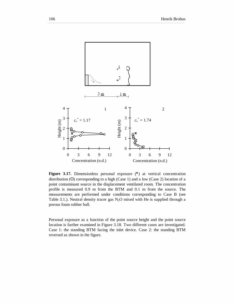
Henrik Brohus106
Figure 3.17. Dimensionless personal exposure (∗∗∗∗) at vertical concentrationdistribution (Ο) corresponding to a high (Case 1) and a low (Case 2) location of apoint contaminant source in the displacement ventilated room. The concentrationprofile is measured 0.9 m from the BTM and 0.1 m from the source. Themeasurements are performed under conditions corresponding to Case B (seeTable 3.1.). Neutral density tracer gas N2O mixed with He is supplied through aporous foam rubber ball.
Personal exposure as a function of the point source height and the point sourcelocation is further examined in Figure 3.18. Two different cases are investigated.Case 1: the standing BTM facing the inlet device. Case 2: the standing BTMreversed as shown in the figure.
0
1
2
3
4
0 3 6 9 12Concentration (n.d.)
Hei
ght (
m)
0
1
2
3
4
0 3 6 9 12Concentration (n.d.)
Hei
ght (
m)
1 2
ce* = 1.74ce
* = 1.17

Chapter 3 Displacement ventilation 107
Figure 3.18. Dimensionless personal exposure, ce*, as a function of point
contaminant source height in the displacement ventilated room. The horizontaldistance between the source and the BTM is 1.5 m. Case 1: BTM facing inletdevice (�). Case 2: BTM reversed (o). The measurements are performed underconditions corresponding to Case B (see Table 3.1.). Neutral density tracer gasN2O mixed with He is supplied through a porous foam rubber ball.
0
1
2
0.5 1.0 1.5Personal exposure (n.d.)
Sou
rce
heig
ht (
m)
Case 1Case 2 ce
* = ce/cR

Henrik Brohus108
Figure 3.18. shows how the exposure clearly varies with the elevation of the pointsource in the room. Both improved as well as deteriorated indoor air qualitycompared with the case of complete mixing is found. A distinct dependence on theflow field stresses the importance of convective mass transfer when pollutantdispersion is addressed (Brohus and Nielsen, 1994a). In Case 2 where the BTM,still facing the source located 1.5 m away, is turned around the exposure is almostopposite to Case 1, as if mirrored in the ordinate axis of Figure 3.18. In the onecase the horizontal convective flow removes or dilutes the contamination, eithergiving rise to improved conditions (ce
* < 1) or somewhat "mixed" conditions (ce* ~
1) in the lower zone. In the other case the horizontal convective flow transportsthe contamination directly against the manikin where a fraction is entrained in theboundary layer giving rise to enhanced exposure (ce
* > 1). Actually, this resultmay to some extent be expected when the stratified flow is considered with a mainflow at the floor, reverse flow above, etc.
In Figure 3.19. a similar experimental set-up is used but now the BTM is seated.The results in Figure 3.19. show a generally lower exposure level in Case 2 but,otherwise, the same tendencies are found as regards Figure 3.18.

Chapter 3 Displacement ventilation 109
Figure 3.19. BTM seated, otherwise the conditions are the same as mentioned inFigure 3.18.
To illustrate the route of the contaminant in the boundary layer measurements areperformed on the contaminant concentration at the chest and the contaminantconcentration at the back in proportion to the point source height, see Figure 3.20.The conditions are otherwise the same as in Figure 3.18., Case 2.
0
1
2
0.5 1.0 1.5Personal exposure (n.d.)
Sou
rce
heig
ht (
m) Case 1
Case 2
ce* = ce/cR

Henrik Brohus110
Figure 3.20. Dimensionless concentrations measured at the chest (o) and at theback (�) at a distance of 0.3 m from a virtual point between the ears of the BTM.The concentrations are found as a function of the vertical location of the pointcontaminant source. The conditions are otherwise the same as in Figure 3.18.,Case 2.
0
1
2
0.5 1.0 1.5
Concentration (n.d.)
Sou
rce
heig
ht (
m)
ChestBack
c* = c/cR
Chapter 3 Displacement ventilation 111
The concentration at the two points in Figure 3.20. are measured at the sameheight in the room. If the Breathing Thermal Manikin was not present they wouldbe approximately the same, while in the actual case there is a significantdifference. What makes the difference is the presence of a person and theentrainment and transport of the contaminant as well as the fresh air in theboundary layer.
If the concentration at the chest is compared with the personal exposure in Figure3.18., Case 2, a very good correspondence is seen. This is due to the fact that themain part of the inhaled air comes from the boundary layer in front of the person,anyhow, in the case of an almost motionless person, unaffected by obstacles in aroom, where the velocities from the air distribution system are sufficiently low toavoid draught and to ensure thermal comfort.
The measurements show a significant influence of the person’s orientation relativeto the flow field and relative to the passive point contaminant source. If the BTMis turned around to face the inlet, the exposure may presumably be reduced by25% in the present case.
If a contaminant source (passive as well as non-passive) is located close to aperson, e.g. in the occupant’s hands or on the desk top, very high exposures maybe obtained. In this case personal exposure depends to a large extent on local flowphenomena around the person and the source (Brohus and Nielsen, 1995). InFigure 3.21. the personal exposure to a point contaminant source located close tothe BTM is examined for standing position and seated position, respectively.

Henrik Brohus112
Figure 3.21. Dimensionless personal exposure, ce*, for different locations of a
passive point contaminant source located close to the standing BTM (top) and theseated BTM (bottom). The measurements are performed under conditionscorresponding to Case B (see Table 3.1.). Neutral density tracer gas N2O mixedwith He is supplied through a porous foam rubber ball. The horizontal distancesshown in the figure correspond to the distance from the front edge of the mouth tothe centre of the source.
Figure 3.21. clearly illustrates the effect of entrainment in the human convectiveboundary layer and stresses the importance of taking it into consideration whensignificant local gradients in the concentration field prevail. For instance, wherethe BTM is seated we see that for the point source located just in front of the

Chapter 3 Displacement ventilation 113
head, at a horizontal distance of 0.25 m the dimensionless concentration is 6.4.When the source is lowered by approximately half a metre, the exposure isactually doubled due to entrainment along the legs and the trunk.
Personal exposure index in displacement ventilated rooms
In the figures shown above, all concentrations are made dimensionless by dividingby the return concentration, cR. Consequently, the personal exposure index, εe, iseasily obtained as the inverse of the dimensionless exposure.
If the room air is fully mixed, both the dimensionless personal exposure, ce*, and
the personal exposure index, εe, equal 1. When the exposure decreases due toimproved indoor air quality, εe exceeds 1. This is the typical case in displacementventilated rooms, see Figure 3.22.
Figure 3.22. Personal exposure index, εe, as a function of the dimensionlessheight yst/ye (relative stratification height). The results correspond to those shownin Figure 3.12. The personal exposure index in case of complete mixing isindicated by the dotted line, i.e. εe = 1.
0
5
10
0.0 0.5 1.0
Relative stratification height (n.d.)
Per
sona
l exp
osur
e in
dex
(n.d
.)
yst/ye
εe

Henrik Brohus114
In Figure 3.22., εe is plotted as a function of yst/ye for the measurementscorresponding to Figure 3.13. The dotted line indicates complete mixing. Theresults show how the displacement principle improves the air quality comparedwith dilution ventilation. In practice, the results will appear less significant due topersons' movements and other disturbances in a displacement ventilated room asdiscussed previously.
One of the advantages of using εe, compared to for example the ventilationeffectiveness in the occupied zone, is the fact that the personal exposure indexrelates to what is actually experienced by a person and not just a kind of "mean"air quality. If εe is known, we may, as a first step, treat the ventilated room asfully mixed. The personal exposure index is then used to convert the "fully mixedexposure" into "actual exposure" when the mean concentration is divided by εe
(Brohus and Nielsen, 1996c).
3.4. Measurements using a TSP
The results shown in the preceding chapter are all chemical measurementsperformed at steady-state conditions. Consequently, the results apply mainly formid-term and long-term exposure assessments. Perceived air quality, however, isdefined as the immediate impression of the indoor air quality experienced by thepeople entering a room (Fanger, 1988). In that case it is crucial to consider thetransient phenomena which occur when people are entering a room causingdisturbances, while they are inhaling room air and judging the air quality.
In this chapter results will be presented which are highly transient. Here, the airquality in a displacement ventilated room will be determined by a Trained SensoryPanel (TSP) together with chemical measurements. This implies that the personalexposure in the present measurements is found directly by asking humans.
One of the objectives of the measurements is to examine whether the improved airquality in displacement ventilated rooms found by long-term chemicalmeasurements, can be confirmed in the short-term case applying the concept ofperceived air quality. Some measurements on the entrainment and transport offresh air in the human convective boundary layer will also be presented anddiscussed.

Chapter 3 Displacement ventilation 115
3.4.1. Experimental set-up
Facilities
The measurements are performed in a test room of stainless steel with a floor areaof 9 m2 and a height of 2.5 m, see Figure 3.23. Subcooled air is supplied througha perforated floor and exhausted through four openings in the ceiling. The supplyair temperature is controlled to keep the air temperature in the breathing zoneheight close to 22°C during the experiments. Five light bulbs of 100 W located0.1 m above the floor constitute the heat sources.
Figure 3.23. Location of heat sources (H) and contaminant sources (C) in thedisplacement ventilated full-scale test room. Measurement location for the verticalconcentration and temperature profiles (M). A large stop watch is located at (S).The route of the subjects is shown by the dotted line. The bold line on the routeshows where the subjects do the assessment. The room height is 2.5 m.

Henrik Brohus116
Figure 3.24. Sensory and chemical contaminant source used in the presentmeasurements. The source consists of 2-propanone generated by passiveevaporation from liquid phase in a 3 litre glass jar. The gaseous contaminant istransported from the glass jar to the test room by means of a pump and a tube, ø0.01 m. The 2-propanone is delivered by the tube with an initial upward velocity.Then it is contained and transported to the upper part of the test room in theplume of ascending air formed by a hot light bulb (100 W) located below thetubes, see photos in Figure 3.25. Two identical sources are used in theexperiments, both supplied from the same glass jar by means of a T-junction. Thelocation (C) is shown in Figure 3.23.
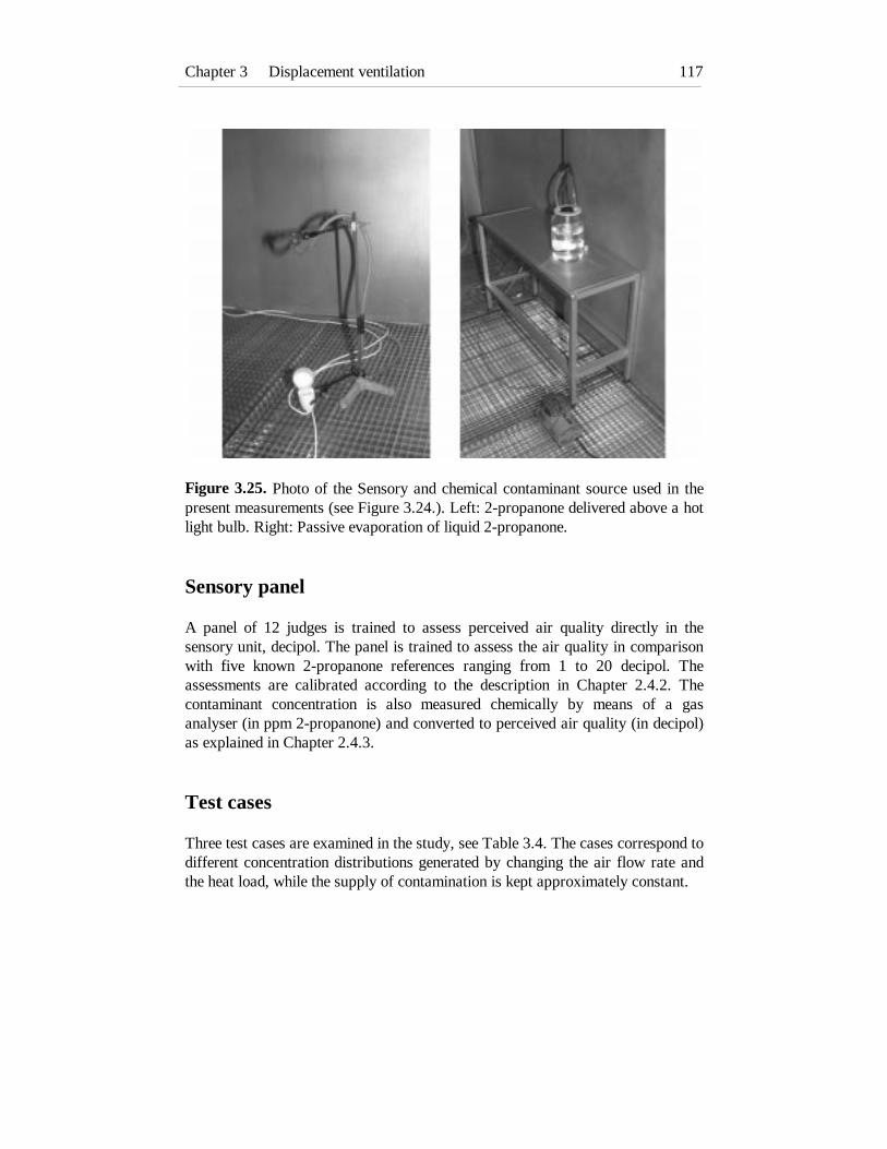
Chapter 3 Displacement ventilation 117
Figure 3.25. Photo of the Sensory and chemical contaminant source used in thepresent measurements (see Figure 3.24.). Left: 2-propanone delivered above a hotlight bulb. Right: Passive evaporation of liquid 2-propanone.
Sensory panel
A panel of 12 judges is trained to assess perceived air quality directly in thesensory unit, decipol. The panel is trained to assess the air quality in comparisonwith five known 2-propanone references ranging from 1 to 20 decipol. Theassessments are calibrated according to the description in Chapter 2.4.2. Thecontaminant concentration is also measured chemically by means of a gasanalyser (in ppm 2-propanone) and converted to perceived air quality (in decipol)as explained in Chapter 2.4.3.
Test cases
Three test cases are examined in the study, see Table 3.4. The cases correspond todifferent concentration distributions generated by changing the air flow rate andthe heat load, while the supply of contamination is kept approximately constant.

Henrik Brohus118
Table 3.4. Specification of the three test cases. q is the supply air flow rate, n isthe air change rate, Φ is the heat load, t0 is the supply air temperature, and tR isthe return air temperature. The heat load is generated by five 100 W light bulbs inCase 1 and Case 2. In Case 3 only the light bulbs below the two contaminantsources are switched-on.Case Parameters
No. of subjects q(m3/h)
n(h-1)
Φ(W)
t0(°C)
tR(°C)
123
121112
263473572
122125
500500200
17.418.720.2
23.122.322.5
The heat load and the air flow rate are chosen to obtain different concentrationdistributions, corresponding to stratification heights below as well as above thebreathing zone height. The average height of the panel is 1.79 m, corresponding toa breathing zone height of approximately 1.6 m.
Procedure
The experiment is performed over three days, one case a day, where the subjectsof the panel assess the perceived air quality one by one. There is an interval ofapproximately 15 minutes between each assessment to ensure that the flow fieldand the contaminant distribution are re-established. The subjects are told to walkin a usual, calm speed and to follow a certain predetermined route in the roomindicated in Figure 3.23. When they pass a certain location in the middle of theroom they do the assessment and walk out of the room again. The door to the testroom is operated by another person to ensure minimum disturbance of the flowfield before entering the room.
The vertical profile of 2-propanone in the room is measured chemically bothduring the assessments as well as over a longer period with the same set-up butwithout the panel (see Figure 3.27.)

Chapter 3 Displacement ventilation 119
3.4.2. Perceived air quality in a displacement ventilatedroom
The vertical temperature distribution in the displacement ventilated room for thethree test cases is shown in Figure 3.26. The temperature profiles are recordedduring the assessments.
Figure 3.26. Dimensionless vertical temperature distribution in the displacementventilated test room in Case 1, 2 and 3 during the assessments. The supplytemperature, t0, and the return temperature, tR, for the three cases are summarisedin Table 3.4. The measurement location (M) is shown in Figure 3.23.
0.0
0.5
1.0
1.5
2.0
2.5
0.0 0.5 1.0
Temperature (n.d.)
Hei
ght (
m)
Case 1Case 2Case 3
tt t
t tR
* =−−
0
0

Henrik Brohus120
As seen in Figure 3.26. the temperature distribution in Case 1 looks like the onesfound in Figure 3.7. with a relatively high gradient in the lower part of the roomand almost no gradient in the upper part. In Case 2 the gradient is reduced, and inCase 3 with a low heat supply and a very high air change rate the gradient isalmost disappeared, which is also expected.
Figure 3.27. shows the vertical contaminant concentration in the three test casesmentioned in Table 3.4. The concentration profiles are expected to berepresentative for the whole room except in the close vicinity of the contaminantsources and in the air current just above, i.e. no significant, horizontalconcentration gradient is expected to prevail in the displacement ventilated room(Nielsen, 1993).
In Figure 3.28. the concentration distribution for the three cases is summarised ina dimensionless plot.

Chapter 3 Displacement ventilation 121
Figure 3.27. Vertical concentration profiles measured chemically for Case 1, 2and 3 during the periods of assessment (TSP present, ∆), and during a longerperiod of approximately 12 hours (no TSP, Ο). The perceived air quality assessedby the TSP is also shown for the approximate breathing zone height of 1.6 m (∗∗∗∗).The measurement location (M) is shown in Figure 3.23.
0.0
0.5
1.0
1.5
2.0
2.5
0 25 50 75 100
Concentration (decipol)
Hei
ght (
m)
Case 1Case 1 (no TSP)
0.0
0.5
1.0
1.5
2.0
2.5
0 20 40 60Concentration (decipol)
Hei
ght (
m)
Case 2Case 2 (no TSP)
0.0
0.5
1.0
1.5
2.0
2.5
0 10 20 30
Concentration (decipol)
Hei
ght (
m)
Case 3Case 3 (no TSP)

Henrik Brohus122
Figure 3.28. Dimensionless vertical concentration profiles in Case 1, Case 2 andCase 3. The results correspond to measurements without the TSP, performed overa longer period of approximately 12 hours. The concentrations are madedimensionless by dividing by the return concentration, c* = c/cR.
The significant concentration peaks in Case 1 and Case 2 are found to exceed theexhaust concentration by a factor of approximately two. The reason may be thatthe contaminated convection currents are not the warmest as indicated in Figure3.2.
Table 3.5. shows the results of the assessments of the Trained Sensory Panel andthe exhaust air quality in sensory units as well as in chemical units.
The concentration measurements show a highly stratified flow with a very lowconcentration at the floor level increasing strongly with the height. A significantseparation of the cleaner, lower part of the room and the upper, morecontaminated part is found. The stratification height is seen to range from a levelbelow the breathing zone height (Case 1, Figure 3.27.) to a level above thebreathing zone height (Case 3, Figure 3.27.).
0.0
0.5
1.0
1.5
2.0
2.5
0.0 0.5 1.0 1.5 2.0 2.5
Concentration (n.d.)
Hei
ght (
m)
Case 1Case 2Case 3
c* = c/cR

Chapter 3 Displacement ventilation 123
Table 3.5. Upper part, sensory units: Perceived air quality assessed by the TSP,and exhaust air concentrations measured chemically and then converted toperceived air quality. Lower part, chemical units: Personal exposure, ce,determined by the TSP in sensory units and then converted to ppm 2-propanone,exhaust air concentration, cR, and the personal exposure index, εe.
Sensory unitsCase Perceived air quality
(decipol)Exhaust air quality
(decipol)123
1886
472329
Chemical unitsCase ce
(ppm)cR
(ppm)εe
(n.d.)123
793324
209103128
2.63.15.3
A good correspondence is seen if the measurements without the TSP in the roomare compared with the measurements where the subjects visited the room one byone. This indicates that the flow has been stable during the experiments and thatthe subjects have been exposed to almost the same indoor environment in the testroom.
This is a typical example of concentration distributions in a displacementventilated room. If the room had been ventilated after the mixing principle, theconcentrations would be uniform and equal to the exhaust concentrationsmentioned in Table 3.5. in the ideal case. This reveals a high ventilationeffectiveness in the occupied zone with a local concentration significantly belowthe exhaust concentration.
An important objective of the present experiment was to see if the high ventilationeffectiveness measured chemically also applied when humans are asked directlyabout how they perceive the air quality. The measurements show that theperceived air quality in the displacement ventilated room is substantially betterthan in case of mixing ventilation (see Table 3.5.). The concentration measured indecipol is assessed to be 3 - 5 times lower than in case of mixing ventilation. Forinstance, in Case 3 the TSP assesses the air quality to be 6 decipol when the

Henrik Brohus124
concentration in the exhaust air is 29 decipol. This difference exceeds the usualventilation effectiveness found in displacement ventilated rooms (ECA, 1992).
If the personal exposure, ce, is compared with the concentration measured at a“neutral” point at breathing zone height, cP, in Figure 3.27., it is found that ce ≈ cP
in Case 2 and Case 3, while ce is significantly lower than cP. in Case 1.
This indicates that the assumptions in Chapter 3.3.3. on exposure duringmovements through a concentration field are reasonable, but it also indicates thatdeviations may occur. The reason for the deviation in Case 1 requires furtherinvestigation, but it may be caused by a damming up along the torso of cleaner airfrom the lower part of the room, or it may be due to local differences incontaminant concentrations, which is especially important in situations like Case1 where significant concentration peaks occur in breathing zone height.
In this experiment the disturbances of the flow field in the test room areminimised. Apart from the subjects of the TSP and the door operation nodisturbances took place. In a real room there will be frequent disturbances fromoccupants, openings of doors, cold downdraught from windows, etc. At the sametime the efficiency of the ventilation system will presumably be lower than in thiscase, where the clean air is supplied through the entire perforated floor and the airchange rates are very high. The combined effect of these parameters will be alower personal exposure index and thereby a worse perceived air quality inpractice.
Despite the inevitable differences between laboratory measurements and theconditions in a ventilated room in practice the results are promising. Thisindicates that the improved indoor air quality found in displacement ventilatedrooms using chemical long-term measurements may be confirmed by askinghumans directly (Brohus et al., 1996).
3.4.3. Effect of entrainment in the human boundary layer
The Trained Sensory Panel has also been used to examine if it is possible to showan effect of entrainment and transport of cleaner air in the human convectiveboundary layer in stratified surroundings by asking humans directly. This task isquite difficult due to the transient phenomena involved using humans in contraryto the steady-state measurements performed by means of the Breathing ThermalManikin.

Chapter 3 Displacement ventilation 125
Procedure
The subjects of the TSP are told to walk in a usual, calm speed and to follow apredetermined route in the test room. When they arrive to a location in the middleof the room they have been told to stop, stand still, and wait for 15 seconds whileholding the breath (looking at the stop watch shown in Figure 3.29.), and then dothe assessment and walk out of the room again. The subjects exhale before theyenter the room. Otherwise, the procedure is like the previous one described inChapter 3.4.2.
This experiment is carried out in combination with the previous one in arandomised way due to requirements of the statistical tests that are performed.This implies that the subjects of the panel will do two different assessments foreach of the three cases in random order.
Results
The three cases mentioned in Table 3.4. are examined together with ameasurement performed without contamination. In Table 3.6. the results aresummarised.
Table 3.6. Mean values of calibrated judgements made by the TSP in the case ofassessments by means of the immediate impression, and after holding the breathfor approximately 15 seconds. Location of subjects while judging and the overalltemperature and contaminant distributions are similar for the two differentapproaches.
Case Immediate impression(decipol)
After holding the breath(decipol)
123
No contamination
18.28.16.03.4
16.75.34.42.4

Henrik Brohus126
Figure 3.29. Member of the TSP standing still in the middle of the displacementventilated test room. She is holding her breath for approximately 15 secondsbefore doing the assessment. In a corner of the room a large stop watch is located,see Figure 3.23. In the bottom of the photo some of the heat sources can be seen.
As seen in Table 3.6., the mean values of the perceived air quality “after holdingthe breath” are all smaller than for the “immediate impression”. This indicates apossible tendency of a lower personal exposure, i.e. a better indoor air quality dueto the ascending air current along the body. However, the mean values do notdiffer much and a statistical test has been performed to check the hypothesis:Concentration assessed after holding the breath is significantly lower than theconcentration assessed by the immediate impression.
A paired t-test has been made assuming random sampling and blocking with pairsin persons. In Table 3.7. the result of the test is summarised. Further details arefound in Appendix F.

Chapter 3 Displacement ventilation 127
Table 3.7. Results of a statistical test of the hypothesis: Concentration assessedafter holding the breath is significantly lower than the concentration assessed bythe immediate impression. Measurements are performed by a TSP in thedisplacement ventilated test room described in Chapter 3.4.1.
Test of hypothesisCase Significant at level
123
No contamination
40%5%25%1%
The levels of significance indicate that only in Case 2 there is a significant effect(5% level) of the convective boundary layer flow along the persons, while thedifferences in Case 1 and Case 3 are insignificant. Furthermore, in case of anuncontaminated test room the hypothesis holds the best, which is quiteunexpected.
This seems to show that the subjects dislike to hold the breath and, therefore, tendto vote too low (i.e. for a better air quality) when they were allowed to inhaleagain. This point is supported by the fact that most members of the TSP do theassessment after only 10 - 15 seconds, in stead of precisely 15 seconds.
Another possible reason for the insignificant results is the highly transientphenomena involved, compared with the short time allowed for the convectiveboundary layer to build up. When a subject is entering the room and walking tothe middle before standing still, a lot of disturbances and vortices are created.While the disturbances are reduced by dispersion and dissipation, the boundarylayer has to build up in about 10 seconds. If the velocity of the ascending aircurrent is assumed to be of the order of 0.2 m/s, this time period corresponds tothe approximate transport time of air from the floor area to the breathing zone.However, this does not include time to re-establish the boundary layer or toovercome eventual vortices or small movements made by the standing person.
In conclusion it must be stated that the time span, during which the subjects areable to hold their breath, is too short to show any significant effect of ascendingair currents along the body. At the same time there seems to be a strongconfounding effect of the restricted respiration where the panel tends to vote toolow when allowed to inhale again.

Henrik Brohus128
3.5. Simulations using a CSP
This chapter presents results from CFD-simulations on personal exposure in adisplacement ventilated room. The computer simulations are performed with bothwarm and cold sources, including a simulation of the floor as a contaminantsource giving rise to exposure of the Computer Simulated Person (CSP) appliedin the calculations. The main results are compared with corresponding full-scalemeasurements.
3.5.1. Geometry and boundary conditions
Three different cases are simulated corresponding to Case A, B and C in the full-scale measurements of Chapter 3.3. The flow field is assumed to be symmetric forwhich reason only one half of the room is simulated in order to save a largenumber of grid points, computer memory and CPU-time, accordingly.
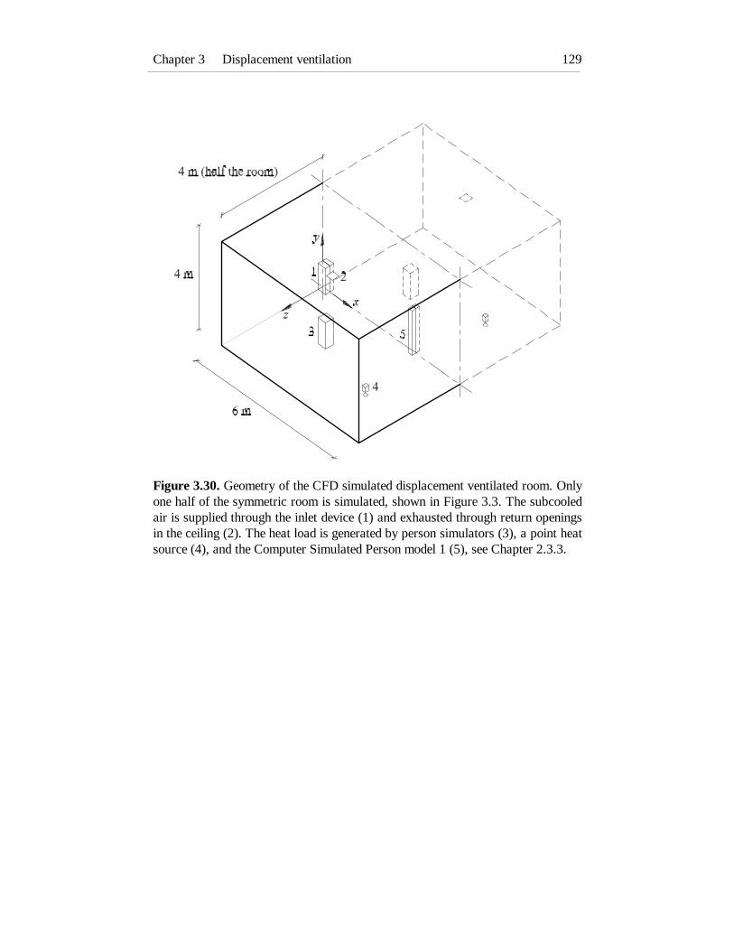
Chapter 3 Displacement ventilation 129
Figure 3.30. Geometry of the CFD simulated displacement ventilated room. Onlyone half of the symmetric room is simulated, shown in Figure 3.3. The subcooledair is supplied through the inlet device (1) and exhausted through return openingsin the ceiling (2). The heat load is generated by person simulators (3), a point heatsource (4), and the Computer Simulated Person model 1 (5), see Chapter 2.3.3.

Henrik Brohus130
The experimental set-up is not symmetrical regarding the point heat source, but inthe simulations this heat source is assumed to consist of two symmetricallylocated heat sources, each emitting half the power of the single one. Thisassumption will be further discussed later.
Due to requirements of the computer software all circular geometry is convertedinto rectangular geometry as seen in Figure 3.30.
Radiation heat transfer is considered indirectly by prescribing the surfacetemperatures of floor, ceiling, and walls using results from the full-scalemeasurements summarised in Table 3.8.
Table 3.8. Boundary conditions used in the CFD simulations. q is the supply airflow rate and t0 is the supply air temperature. The temperatures of the differentsurfaces are also mentioned. Wall functions are used to calculate the heat transferbetween the room air and the surfaces (see Chapter 2.3.2.3.).
Parameter Location Case A Case B Case Cq0 (m
3/h) Supply 145 290 395t0 (°C)tFloor
tCeiling
tFront
tBack
tSide
Supplyy = 0 my = 4 mx = 6 mx = 0 mz = 4 m
14.6722.6323.7023.2222.8722.17
17.6321.9422.4422.4922.2122.42
15.8021.5723.0122.7122.3022.64
The implementation of the heat sources is mentioned in Table 3.9. Only theconvective part of the total heat output should be considered.
Table 3.9. Implementation of the person simulator and the point heat source inthe CFD simulations of the displacement ventilated room.
Type(Case)
Total heatoutput
(W)
Convectiveheat output
(W)
Implementation in theCFD simulations as
Person simulator(A,B,C)
Point heat source(A,C)
Point heat source(B)
100
250
50
50
225
45
Obstacle with prescribedsurface heat flux
Transparent volume source
Transparent volume source

Chapter 3 Displacement ventilation 131
Apart from the two heat sources the Computer Simulated Person (CSP) will alsoact as a heat source in the shape of an obstacle with a prescribed surface heat fluxof 25 W/m2. The CSP is discussed in detail in Chapter 2.3.3. In the presentsimulations only CSP model 1 is applied.
The grid used in the numerical calculations of the three cases consists of 82,764cells distributed with 66, 33 and 38 cells in the x, y, and z direction, respectively.
3.5.2. Simulation of the flow field
Here, the flow field in the three cases will be shown by means of vector plots andcomparisons between measurements and simulations regarding velocity andtemperature profiles in the vicinity of the person.
Figure 3.31., 3.32. and 3.33. show vector plots from three different planes forCase A, B and C.

Henrik Brohus132
Figure 3.31. Vector plot from the displacement ventilated room Case A, B and C.Plane: z = 0 m (vertical symmetry plane).

Chapter 3 Displacement ventilation 133
Figure 3.32. Vector plot from the displacement ventilated room Case A, B and C.Plane: x = 4 m (vertical section through CSP).

Henrik Brohus134
Figure 3.33. Vector plot from the displacement ventilated room Case A, B and C.Plane: y = 0.1 m (horizontal plane 0.1 m above the floor).

Chapter 3 Displacement ventilation 135
Figure 3.31. shows a vector plot from the vertical symmetry plane, z = 0 m. Inthis plane it is possible to see many of the characteristics of a displacementventilated room, especially close to the inlet device and the CSP. The flow aroundthe CSP clearly shows the convective flow causing entrainment and transportalong a person in all three cases. In the adjacent zone of the inlet device the flowfield is influenced by the air flow rate and the temperature difference between thesupply air and the room air, i.e. the Archimedes number.
In the major part of the room the flow direction is horizontal as expected for astratified flow domain. Only close to sources of momentum, like the inlet deviceand the heat sources (CSP, walls, etc.), significant non-horizontal movementsprevail. In the upper right corner of the Case A vector plot downward movementsare created by the point heat source which is not visible in this plane, see Figure3.31.
Figure 3.32. shows a vertical section through the CSP, x = 4 m. Close to the CSPthe ascending air current is seen again continuing to the ceiling where it isdeflected. On top of the CSP a small recirculation zone is formed due to therectangular geometry causing an edge which is sharper than the one found on realpersons. However, in the case of displacement ventilation where the upward airmovement along the body is assumed to be the main route of contamination it isnot likely that this recirculation zone will affect the personal exposuresignificantly.
The differences in the overall flow pattern in Figure 3.32. are due to the differentboundary conditions regarding air flow rate, heat load and surface temperatures.Especially the point heat source seems to affect the flow field considerably in theupper part of the room.
Figure 3.33. consists of three vector plots of the flow field in a horizontal plane0.1 m above the floor, y = 0.1 m. As in Figure 3.31. the flow field close to theinlet device is highly affected by the Archimedes number. As expected, thesubcooled air is seen to spread radially along the entire floor. Behind the person asmall wake is created due to the relatively high velocities close to the floor. Thiswake region can also be seen in Figure 3.31. and it seems to continue up to aheight of approximately 0.2 m where it is gradually diminished.

Henrik Brohus136
Figure 3.34. Velocity profiles (left) and dimensionless temperature profiles (right)for the CFD simulations (line) and full-scale measurements (o) for Case A, B andC for the displacement ventilated room. The location of the vertical velocityprofile is (x,z) = (3,0) and the vertical temperature profile is (x,z) = (4,1). Thetemperature profiles are shown in a dimensionless plot, t* = (t - t0)/(tR - t0), wheret0 is the supply air temperature and tR is the return air temperature.
Case A
0
1
2
-0.1 0.0 0.1 0.2 0.3
Velocity (m/s)
Hei
ght (
m)
Case A
0
1
2
3
4
0.0 0.5 1.0
Temperature (n.d.)
Hei
ght (
m)
Case B
0
1
2
3
4
0.0 0.5 1.0
Temperature (n.d.)
Hei
ght (
m)
Case B
0
1
2
-0.1 0.0 0.1 0.2 0.3
Velocity (m/s)
Hei
ght (
m)
Case C
0
1
2
-0.1 0.0 0.1 0.2 0.3Velocity (m/s)
Hei
ght (
m)
Case C
0
1
2
3
4
0.0 0.5 1.0Temperature (n.d.)
Hei
ght (
m)

Chapter 3 Displacement ventilation 137
The simulated velocity profiles and temperature profiles for locations close theperson are compared with results from the full-scale measurements in Figure3.34. A reasonable agreement is found even though the simulation seems tounderestimate the velocities slightly and the shape of the temperature profilesdeviates somewhat in Case B and Case C. Comparisons between simulations andmeasurements will be discussed in the following chapter where the concentrationdistribution also is included.
3.5.3. Simulation of personal exposure
Simulations on personal exposure have been made using a non-passive (warm)contaminant source as well as two kinds of passive (cold) contaminant sources inthe shape of a point contaminant source and the entire floor. In all cases thepersonal exposure of the Computer Simulated Person (CSP) corresponds to thecontaminant concentration in the nearest cell along the computational model in aheight of 1.5 m as explained in Chapter 2.3.4.
Non-passive point contaminant source
The concentration distribution in the present CFD simulations is generated bymeans of a contaminant source simulated as a transparent volume source (0.1 m x0.1m x 0.1 m) located above the point heat source in a height of 2 m above thefloor. The combination of the point heat source generating an ascending plume ofwarm air and the contaminant source located above causes a transport of thecontamination to the upper part of the room, which is also the aim of this non-passive source.
The dimensionless concentration distribution is shown for Case A in Figure 3.35.The discrete results are converted into isopleths using a computer programmeincorporating Kriging for the interpolations (Surfer, 1991; Davis, 1986).

Henrik Brohus138
Figure 3.35. Dimensionless contaminant concentration distribution in thedisplacement ventilated room, Case A. Top: Vertical symmetry plane, z = 0 m.Bottom: Vertical section through person, x = 4 m. The two right figures areenlargements of the concentration field close to the CSP.
Figure 3.35. shows the concentration field in the ventilated room for two differentvertical planes combined with an enlargement of the field close to the CSP. Theconcentrations are made non-dimensional by dividing by the return concentration,i.e. c* = c/cR, which implies that the dimensionless return concentration equals 1.
The results indicate a stratified flow with horizontal, almost parallel,isoconcentration curves increasing in level for increasing height above the floor.The clean air is supplied by the inlet device in the lower part of the room andsubtracted again at ceiling height. In the plane x = 4 m we see the same local

Chapter 3 Displacement ventilation 139
effect of the point heat source on the concentration distribution, as the one foundin the corresponding vector plot (Figure 3.32.).
Close to the CSP the concentration field is significantly modified due to theconvective transport in the boundary layer. The cleaner air in the lower part of thedisplacement ventilated room is entrained and transported to the breathing zone.This is in fact one of the important reasons for applying the displacementprinciple in room ventilation. This phenomenon causes a high ventilationeffectiveness locally around the person and thus a high personal exposure index,εe, which was also found in the case of full-scale measurements.
The corresponding results for Case B and Case C do not show any importantdifferences from Figure 3.35. for which reason they are not included asisoconcentration plots.
In Figure 3.36. the personal exposure, ce*, and the vertical concentration
distribution in the vicinity of the person are shown for the simulations and themeasurements. The concentration profiles for the simulations clearly indicate astratified flow, but comparison with measurements shows some significantdeviations in the lower part of the room. Obviously, the simulations have not beenable to re-create the considerable “step” in the concentration profiles found in themeasurements. This subject will be discussed in more detail in the end of thischapter.
Even though the CFD calculated concentration distribution reveals somedeviations compared with measurements, the personal exposure shows the sametendencies of a significantly lower concentration of inhaled contaminant than thecorresponding concentration in the surroundings at a “neutral” point.

Henrik Brohus140
Figure 3.36. Vertical dimensionless concentration distribution in the displacementventilated room for Case A, B and C at (x,z) = (3,1) for simulations (line) andmeasurements (o). The personal exposure of a standing person is shown for thesimulations (CSP, ∆) and for the measurements (BTM, ∗). The breathing zoneheight is 1.5 m in both cases.
Case AStanding
0
1
2
3
4
0.0 0.5 1.0 1.5Concentration (n.d.)
Hei
ght (
m)
Case BStanding
0
1
2
3
4
0.0 0.5 1.0 1.5Concentration (n.d.)
Hei
ght (
m)
Case CStanding
0
1
2
3
4
0.0 0.5 1.0 1.5Concentration (n.d.)
Hei
ght (
m)
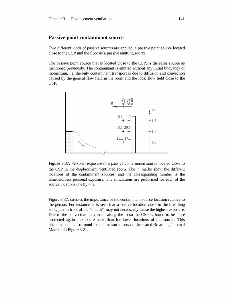
Chapter 3 Displacement ventilation 141
Passive point contaminant source
Two different kinds of passive sources are applied, a passive point source locatedclose to the CSP and the floor as a passive emitting source.
The passive point source that is located close to the CSP, is the same source asmentioned previously. The contaminant is emitted without any initial buoyancy ormomentum, i.e. the only contaminant transport is due to diffusion and convectioncaused by the general flow field in the room and the local flow field close to theCSP.
Figure 3.37. Personal exposure to a passive contaminant source located close tothe CSP in the displacement ventilated room. The + marks show the differentlocations of the contaminant sources, and the corresponding number is thedimensionless personal exposure. The simulations are performed for each of thesource locations one by one.
Figure 3.37. stresses the importance of the contaminant source location relative tothe person. For instance, it is seen that a source location close to the breathingzone, just in front of the “mouth”, may not necessarily cause the highest exposure.Due to the convective air current along the torso the CSP is found to be moreprotected against exposure here, than for lower locations of the source. Thisphenomenon is also found for the measurements on the seated Breathing ThermalManikin in Figure 3.21.
Henrik Brohus142
Planar contaminant source
In the previous examples of exposure to contaminant sources only point sourceshave been applied. For a typical indoor environment planar sources can also bevery important to consider, e.g. walls and floor that may exert a considerablychemical and sensory pollution load on the room (ECA, 1992; Maroni et al.,1995).
A planar contaminant source in shape of the floor is applied in the results shownin Figure 3.38. The floor in this CFD simulation has a constant emission rate.This may be a good approximation for certain types of contaminant sources,while other types are dependent on velocity, temperature, back pressure, etc. andthus require more sophisticated emission models.
The isoconcentration curves in Figure 3.38. show how the clean, subcooled airfrom the inlet device is gradually more and more polluted during the flowthroughout the floor. At the walls, x = 6 m and z = 4 m, the flow is deflected anda secondary opposing flow occurs above the primary flow. The verticalconcentration profile close to the person is shown in Figure 3.39.
This scenery causes a complex local concentration distribution around the CSP,resulting in a dimensionless personal exposure of approximately 1, i.e. the sameexposure level as if the room air was completely mixed.

Chapter 3 Displacement ventilation 143
Figure 3.38. Dimensionless contaminant concentration distribution in thedisplacement ventilated room in case of the floor acting as a planar contaminantsource with a constant emission rate. The flow field corresponds to Case A, seeTable 3.8. Top: Vertical symmetry plane, z = 0 m. Bottom: Vertical sectionthrough person, x = 4 m. The two right figures are enlargements of theconcentration field close to the CSP.

Henrik Brohus144
Figure 3.39. Vertical dimensionless concentration distribution at (x,z) = (3,1) inthe displacement ventilated room in case of the floor acting as a planarcontaminant source with constant emission. The flow field corresponds to Case A,see Table 3.8. The dimensionless personal exposure of the CSP is also shown (∆).
Comparison between measurements and simulations
If the results from measurements and simulations are compared regarding theconcentration distribution, significant deviations are found in the lower part of theroom. As mentioned previously the simulations have not been able to re-create theconsiderable vertical step change in the concentration distribution. There are anumber of possible reasons for the deviations, some of those will be outlined inthe following.
The flow field is determined almost exclusively by the boundary conditions in theCFD calculations. If the boundary conditions are not properly applied deviationswill inevitably occur. In the present simulations the surface temperatures of walls,floor and ceiling are prescribed as a single value for each surface. During themeasurements there may be a temperature gradient throughout the single surfaceswhich is not implemented. This will to some extent affect the convective flowalong the walls and thus it may influence the exchange of contamination betweenthe upper and the lower part of the room.
In Chapter 2.3.3.2. the grid dependence of wall functions applied in the CFDsimulations was discussed. Here, the wall functions are applied to account forsurface friction and heat transfer along the surfaces where the temperature is
Case APlaner source
(floor)
0
1
2
3
4
0.0 0.5 1.0 1.5Concentration (n.d.)
Hei
ght (
m)

Chapter 3 Displacement ventilation 145
prescribed. The grid layout may also exert an influence on the representation ofheat and contaminant sources as well as on the general flow field. For instance, ifthe grid is too coarse in the “step region” the simulations may fail to catch thisimportant property of displacement ventilation.
The turbulence in the flow is represented by turbulent exchange parameters likethe turbulent viscosity. The turbulent viscosity is found by means of the k-ε modelas described in Chapter 2.3.2.1. In strongly temperature-stratified surroundings,the turbulence may be significantly influenced by the temperature gradient.Depending on the sign of the vertical temperature gradient the local turbulencemay be damped or amplified. This phenomenon can be implemented in theturbulence model by the inclusion of a so-called buoyancy term, Gk, in thetransport equation for turbulent kinetic energy, k, see Appendix E.
G gt
xk it
k i
= −βµσ
∂∂
(3.11)
where
Gk = Buoyancy term (J/m3 s)β = Expansivity (1/K)gi = Gravitational acceleration (m/s2)µt = Turbulent viscosity (kg/m s)σk = Turbulent Prandtl number (n.d.)t = Temperature (°C)xi = Distance in i direction (m)
The Gk term may also be included in the transport equation for the rate ofdissipation of turbulent kinetic energy, ε. In both cases it should be included as anadditional source term. The buoyancy term has not been applied in the presentsimulations, but it may be a possibility to obtain better numerical solutions.
Another reason for the deviations between the measurements and the simulationsis the symmetry assumptions. In the measurements there is only one point heatsource, see Figure 3.3., but in the simulations this source is assumed to consist oftwo symmetrical sources, each with only half the power as the single source. Dueto the location of the contaminant source above this heat source in the non-passivecase, the symmetry assumption may have a certain influence on the concentrationdistribution.

Henrik Brohus146
3.6. ConclusionIn this chapter personal exposure to contaminant sources in a displacementventilated room is examined.
The topic is investigated by means of the three tools for exposure assessmentintroduced in Chapter 2, i.e. the Breathing Thermal Manikin, the Trained SensoryPanel and the Computer Simulated Person. The different tools are models of aperson or real persons applied in order to include the local effect of the personwhen the exposure is estimated in surroundings with considerable concentrationgradients.
The contaminant distribution is generated by point sources and also by a planarcontaminant source in the case of CFD simulations including the ComputerSimulated Person. Warm (non-passive) sources are applied to generate thecharacteristic two-zonal concentration distribution with a separation in a cleaner,lower zone and an upper, more contaminated zone in the displacement ventilatedroom. Cold (passive) point contaminant sources are, among other things, appliedin order to investigate the influence of contaminant sources located close topersons.
Both chemical and sensory measurements and simulations are performed, mainlyat steady-state conditions but also by transient behaviour in the shape of theTrained Sensory Panel assessing the perceived air quality.
It is found that the stratified flow and the considerable concentration gradients ina displacement ventilated room necessitate an improvement of the widely usedcompartmental approach.
The flow in the human boundary layer is able, to a great extent, to entrain airfrom below the breathing zone, thus improving the quality of the inhaled air incase of warm contaminant sources.
Persons movements cause the air quality to decrease due to the disturbance of thehuman boundary layer which promotes the high air quality transporting fresh airto the breathing zone.
A personal exposure model is proposed. The model takes the concentrationgradient and the influence of the human thermal boundary layer into account. Themodel is easy-to-use and suitable for the design of displacement ventilationsystems in practice.

Chapter 3 Displacement ventilation 147
Entrainment of air in the human boundary layer is usually an advantage, but theresults show also the possible disadvantage when passive contaminant sources arepresent. In this case the convective current around the person may transportcontaminated air to the breathing zone, giving rise to increased exposure.
A new quantity is defined: the effectiveness of entrainment in the human boundarylayer, ηe, which expresses the ability to supply (fresh) air from the floor area tothe breathing zone.

Henrik Brohus148

Chapter 4 Mixing ventilation 149
Chapter 4
Mixing ventilation
4.1. Introduction
In this chapter mixing ventilation will be examined as an application for personalexposure assessment, using some of the tools introduced in Chapter 2.
Mixing ventilation may cover a large number of ventilation systems and an evenlarger number of different devices used to supply and extract the air. Usually, theair is supplied outside the occupied zone with a high momentum in order to createa well-mixed flow field without any concentration gradients or temperaturegradients in the ideal case. The supply air may be isothermal as well as non-isothermal and used for both heating and cooling and, of course, also for theremoval of contamination and supply of fresh air.
When the mixing principle is used the contamination in a ventilated room isdiluted to a sufficiently low level contrary to the displacement principle, where thecontamination is displaced upwards while clean air is supplied directly to theoccupied zone.
The assumption of completely mixed room air without concentration gradients iswidely used in the design of ventilation systems. Using this approach the personalexposure may easily be found by means of a simple mass balance if the sourcestrength and the air flow rate are known. In a large number of cases, however, theassumption will fail and erroneous exposures may be obtained. Rodes et al.(1991) and Brohus and Nielsen (1995) among others report errors in exposureassessment exceeding one order of magnitude.
In this chapter the topic will be highlighted, and different examples willdemonstrate the importance of taking the local influence of a person into accountwhen personal exposure is assessed in surroundings where concentration gradientsprevail.

Henrik Brohus150
The flow field around persons in mixing ventilated rooms depends highly on thespecific system design and also on the location of the person in the room,movements of the person, local obstacles, heat sources, etc. The flow may rangefrom almost quiescent air over strongly turbulent flow to an almost uniformvelocity field locally around the person, see Figure 4.1.
Figure 4.1. The flow field in a mixing ventilated room may locally act as aunidirectional flow field.
Measurements and computer simulations are performed on a person exposed tocontaminant sources in a unidirectional flow field created by means of a windchannel. The results are presented and discussed in Chapter 4.2.
Chapter 4.3. presents a CFD simulation on the whole flow field in a mixingventilated room and examines the personal exposure as a function of sourcelocations as well as the flow direction relative to the person.
4.2. Unidirectional flow field
As mentioned previously this chapter presents measurements and simulations on aperson located in a unidirectional flow field. The unidirectional flow field isassumed to be part of the total flow field in a mixing ventilated room, as indicatedin Figure 4.1., but it may as well apply for industrial applications, for instance aworker located in a spray hood or close to a local exhaust ventilation device.

Chapter 4 Mixing ventilation 151
4.2.1. Experimental set-up
In order to create a unidirectional flow field a wind channel is built as shown inFigure 4.2.
Figure 4.2. Geometry of wind channel used in the full-scale measurements on theBTM standing in a unidirectional flow field. The flow field is generated byextracting air through two exhaust openings, each ø 0.25 m.
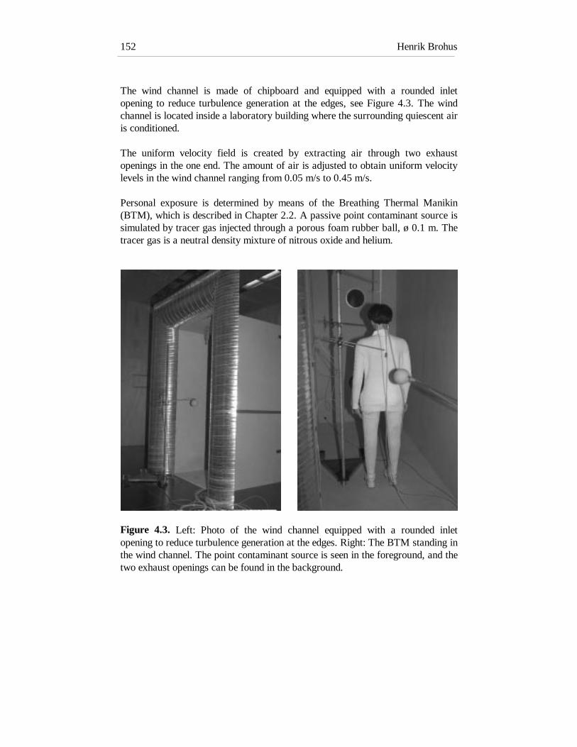
Henrik Brohus152
The wind channel is made of chipboard and equipped with a rounded inletopening to reduce turbulence generation at the edges, see Figure 4.3. The windchannel is located inside a laboratory building where the surrounding quiescent airis conditioned.
The uniform velocity field is created by extracting air through two exhaustopenings in the one end. The amount of air is adjusted to obtain uniform velocitylevels in the wind channel ranging from 0.05 m/s to 0.45 m/s.
Personal exposure is determined by means of the Breathing Thermal Manikin(BTM), which is described in Chapter 2.2. A passive point contaminant source issimulated by tracer gas injected through a porous foam rubber ball, ø 0.1 m. Thetracer gas is a neutral density mixture of nitrous oxide and helium.
Figure 4.3. Left: Photo of the wind channel equipped with a rounded inletopening to reduce turbulence generation at the edges. Right: The BTM standing inthe wind channel. The point contaminant source is seen in the foreground, and thetwo exhaust openings can be found in the background.
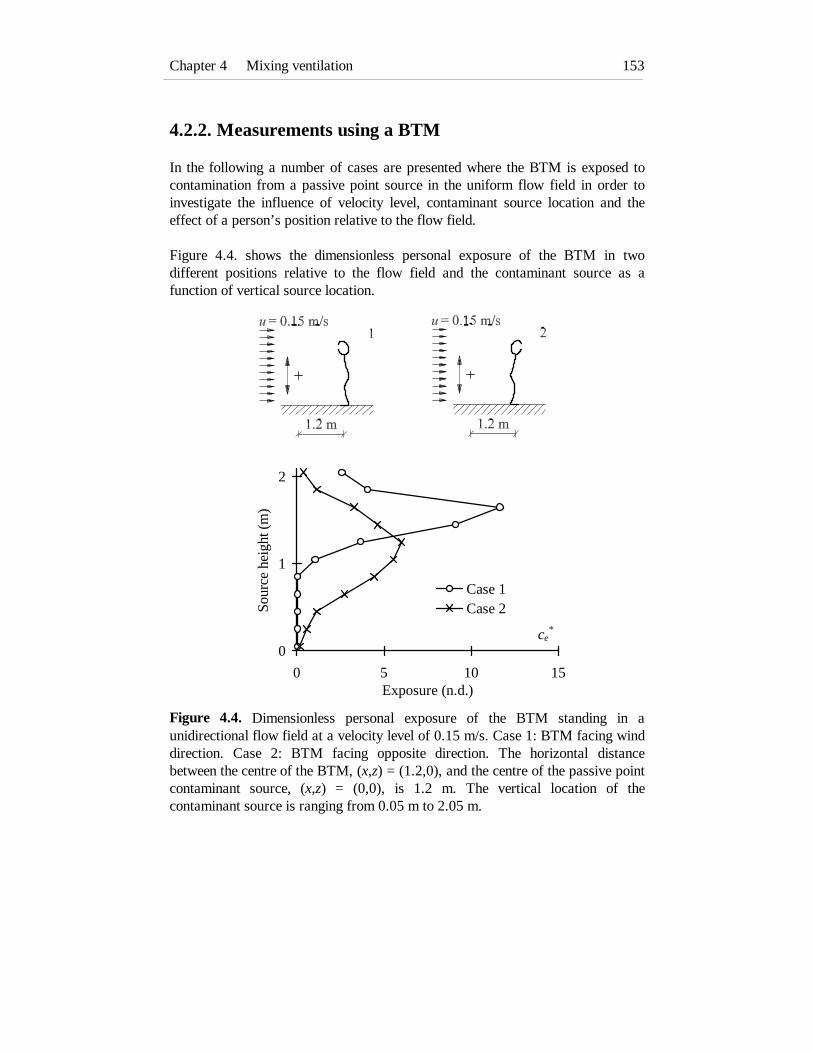
Chapter 4 Mixing ventilation 153
4.2.2. Measurements using a BTM
In the following a number of cases are presented where the BTM is exposed tocontamination from a passive point source in the uniform flow field in order toinvestigate the influence of velocity level, contaminant source location and theeffect of a person’s position relative to the flow field.
Figure 4.4. shows the dimensionless personal exposure of the BTM in twodifferent positions relative to the flow field and the contaminant source as afunction of vertical source location.
Figure 4.4. Dimensionless personal exposure of the BTM standing in aunidirectional flow field at a velocity level of 0.15 m/s. Case 1: BTM facing winddirection. Case 2: BTM facing opposite direction. The horizontal distancebetween the centre of the BTM, (x,z) = (1.2,0), and the centre of the passive pointcontaminant source, (x,z) = (0,0), is 1.2 m. The vertical location of thecontaminant source is ranging from 0.05 m to 2.05 m.
0
1
2
0 5 10 15Exposure (n.d.)
Sou
rce
heig
ht (
m)
Case 1Case 2
ce*

Henrik Brohus154
The results are presented in dimensionless form regarding the personal exposureto make them more general and independent of the specific source strength chosenfor the experiments. Another advantage of showing the results dimensionless isthe ability to compare with completely mixed conditions, where ce
* equals one.However, if the dimensionless exposure is used for physiological purposes, forinstance as input in a dose-response relationship, the concentration of a specificgas must be converted to ppm or other relevant units. When the source strength,S, and the air flow rate, q, are known this may easily be done by
c c cc S
qe e Re= =**
(4.1)
As expected, the measurements in Figure 4.4. show a substantial influence of thesource location and they also show a significant influence of the position of themanikin.
In Case 1 no exposure takes place when the source is below 1 m. When the sourceis raised above 1 m the level increases to a maximum value around the breathingzone height, after which it decreases again. The maximum personal exposure isfound to exceed the return concentration more than 10 times.
Case 2 shows a different pattern. Exposure occurs for almost every sourcelocation, and the location for maximum exposure is found at a lower level. Here,we see a distinct influence of the flow in the wake of a person standing in auniform velocity field, a topic that will be examined in greater detail in thesubsequent.
Figures 4.5., 4.6. and 4.7. present a more systematic investigation of the personalexposure as a function of velocity level and vertical location of the contaminantsource in three different set-ups, all highly influenced by the wake generated infront of the BTM standing in a unidirectional flow field.
Each of the three figures shows results of exposure measurements at four velocitylevels (0.05 m/s, 0.15 m/s, 0.30 m/s, 0.45 m/s) and five vertical source locations(0.50 m, 0.75 m, 1.00 m, 1.25 m, 1.50 m), i.e. 20 data points. The results areconverted into isopleths by using a computer programme incorporating Krigingfor the interpolation (Surfer, 1991; Davis, 1986).

Chapter 4 Mixing ventilation 155
The results are presented both in the ppm unit assuming a specific contaminantsource strength as well as non-dimensional. In that way it is possible to commenton the exposure levels compared to complete mixing in a general way, and also tocomment on the physiological effect on people where it is the absolute exposurelevel which counts.
Figure 4.5. Personal exposure of the BTM standing in a uniform velocity field asa function of velocity level (0.05 m/s - 0.45 m/s) and vertical contaminant sourceheight above the floor (0.5 m - 1.5 m). The horizontal distance between the centreof the BTM, (x,z) = (0.7,0), and the centre of the source, (x,z) = (0,0), is 0.7 m.The left plot is isopleths of personal exposure in ppm for a contaminant sourcestrength of S = 5⋅10-6 m3/s. The right plot is isopleths of the correspondingdimensionless personal exposure.
The contours in Figure 4.5. confirm the tendency found in Figure 4.4., Case 2,with the highest exposure level for the contaminant source located approximately

Henrik Brohus156
1 m above the floor. On the dimensionless plot (right side) an almost unchangedexposure level is found for increasing velocity levels, resulting in decreasingabsolute levels (left side) due to the constant source strength.
It can also be seen that the exposure increases significantly when the uniformvelocity is changed from 0.05 m/s to 0.15 m/s. This may be explained by anincreased disturbance of the natural convection boundary layer around the BTM,which in this case seems to protect against exposure at low velocities.
Figure 4.6. Personal exposure of the BTM standing in a uniform velocity field asa function of velocity level (0.05 m/s - 0.45 m/s) and vertical contaminant sourceheight above the floor (0.5 m - 1.5 m). The horizontal distance between the centreof the BTM, (x,z) = (0.7,0), and the centre of the source, (x,z) = (0.95,0), is 0.25m. The left plot is isopleths of personal exposure in ppm for a contaminant sourcestrength of S = 5⋅10-6 m3/s. The right plot is isopleths of the correspondingdimensionless personal exposure.

Chapter 4 Mixing ventilation 157
The set-up in Figures 4.6. and 4.7. are typical examples of locations of hand-heldcontaminant sources located close to the person, for instance in relation to aworking process. It may take place in industrial applications like a spray hood orclose to local exhaust ventilation devices, or it may be a person located in aventilated office where the recirculating flow locally generates the field. Here, thecontaminant source could be an ashtray or some kind of office equipment, etc.
If the exposure levels in Figure 4.5. and Figure 4.6. are compared, a remarkableincrease is found when the source is located downstream the person. The reasonfor the significant increase must be found in the wake generated in front of theperson. The wake consists of a mixture of turbulent diffusion and vortices with aconsiderable ability to entrain contaminant from a certain horizontal distance.This contamination is transported to the boundary layer and the breathing zonewhere it causes exposure (George et al., 1990; Brohus and Nielsen, 1994b; 1995).This is also verified by using smoke visualisation during the experimental work.
The dimensionless exposure in Figure 4.6. indicates a maximum level found for asource location between 1.00 m and 1.25 m above the floor. Furthermore, it isseen that the dimensionless exposure increases for increasing velocity levels,resulting in almost unchanged exposure levels in ppm, i.e. no improvement of theair quality for increased air flow rates.
A dimensional exposure, ce*, around 50 results in a personal exposure index εe =
0.02, which is extremely low and reveals that this source location relative to theperson and the flow field may be rather critical. Unfortunately, this is in fact thecase in a number of industrial applications, where the location actually waschosen in order to remove the contaminants efficiently (Kim and Flynn, 1991b;Ljungqvist and Reinmüller, 1993).
Treating the ventilated enclosure as fully mixed will result in ce* = 1 for all source
locations and velocity levels. This may be compared with a measured personalexposure ce
* > 50 in this case.

Henrik Brohus158
Figure 4.7. Personal exposure of the BTM standing in a uniform velocity field asa function of velocity level (0.05 m/s - 0.45 m/s) and vertical contaminant sourceheight above the floor (0.5 m - 1.5 m). The horizontal distance between the centreof the BTM, (x,z) = (0.7,0), and the centre of the source, (x,z) = (1.2,0), is 0.5 m.The left plot is isopleths of personal exposure in ppm for a contaminant sourcestrength of S = 5⋅10-6 m3/s. The right plot is isopleths of the correspondingdimensionless personal exposure.
The horizontal distance between the contaminant source and the BTM isincreased from 0.25 m to 0.5 m in Figure 4.7. This results in a reduction of theexposure level with a factor of approximately two in general, and locally evenmore, but still significantly higher than the one in Figure 4.5.
If the left plot (in ppm units) is examined there seem to be two differentmechanisms causing high exposure levels. At a low velocity and a high sourcelocation the contamination may be dispersed by diffusion and entrained in thehuman convective boundary layer, where it is transported to the breathing zone

Chapter 4 Mixing ventilation 159
and causes exposure. When the velocity is increased the natural boundary layer isdisturbed and the primary mechanism of contaminant dispersion may beentrainment due to vortices and turbulent diffusion in the wake generated in frontof the BTM.
The momentum supplied by the unidirectional flow field around the person is thedriving force on the vortices. Increased momentum may increase both the strengthof the vortices and the turbulent diffusion. This topic is discussed in more detail inChapter 4.2.3. where the corresponding CFD simulations are presented.
The effect of BTM heating
One of the important features of the Breathing Thermal Manikin is the heatedsurface. This was shown to be a very important factor to consider in the case ofpersonal exposure assessment in a displacement ventilated room. In the followingsome measurements on the effect of a heated surface in a uniform flow field arepresented.
Figure 4.8. shows only a small and insignificant effect of heating at 0.15 m/s forthe BTM facing the flow field and the contaminant source.
In Figure 4.9., however, concentration measurements performed at the back (inthe wake region) indicate a stronger influence of surface heating. Presumably thiseffect will be even more significant at velocity levels below 0.15 m/s.

Henrik Brohus160
Figure 4.8. Dimensionless personal exposure of the BTM standing inunidirectional flow field at a velocity level of 0.15 m/s with the surface heatingturned on (∆) and off (o). Otherwise, same set-up as in Case 1 in Figure 4.4.
0
1
2
0 5 10 15
Exposure (n.d.)
Sou
rce
heig
ht (
m)
Heating ONHeating OFF

Chapter 4 Mixing ventilation 161
Figure 4.9. Dimensionless concentration measured at the back of the BTMlocated in a unidirectional flow field at a velocity level of 0.15 m/s. The resultsare shown for the heating turned on (∆) and off (o). Otherwise, same set-up as inCase 1 in Figure 4.4.
In Figure 4.10. the exposure is found for a fixed source location and four differentvelocity levels ranging from 0.05 m/s to 0.45 m/s. The measurements areperformed with the surface heating turned on and off.
0
1
2
0 5 10Exposure (n.d.)
Sou
rce
heig
ht (
m)
Heating ONHeating OFF

Henrik Brohus162
Figure 4.10. Dimensionless personal exposure of the BTM standing in aunidirectional flow field at four different velocity levels (0.05 m/s, 0.15 m/s, 0.30m/s, 0.45 m/s) in case of the surface heating turned on (∆) and off (o). Thelocation of the BTM is (x,z) = (0.7,0) and the fixed point contaminant source(x,y,z) = (1.0,1.15,0).
The two curves and the corresponding standard deviations for the measuringpoints shown in Figure 4.10. indicate a possible effect of heating at the lowvelocity, and an insignificant effect of heating at the higher velocities, which wasalso to be expected (Brohus and Nielsen, 1994a; Hyldgaard, 1994).
The error bars represent one standarddeviation around the mean value
0
25
50
75
0 0.1 0.2 0.3 0.4 0.5Velocity (m/s)
Exp
osur
e (n
.d.)
Heating ONHeating OFF

Chapter 4 Mixing ventilation 163
Dimensionless numbers
Some of the dimensionless numbers mentioned in Chapter 2.2.2. are calculatedfor the present measurements and shown in Table 4.1
Table 4.1. Dimensionless numbers characterising the flow around the BTMstanding in a unidirectional flow field in the wind channel shown in Figure 4.2. Reis the Reynolds number, Gr is the Grashof number and Ar is the Archimedesnumber. Expressions for the numbers are found in Chapter 2.2.2.
Uniform velocity level Dimensionless numbersu
(m/s)Re
(n.d.)Gr⋅109
(n.d.)Ar
(n.d.)0.050.150.300.45
1000300060009000
4.03.93.53.5
124.413.63.01.3
If the size of the three dimensionless numbers is compared with the levels stated inChapter 2.2.2., it can be concluded that the flow around the Breathing ThermalManikin is laminar at each of the four velocity levels (Re < 2⋅105). The convectiveflow in the boundary layer is found to be in the transition region between thelaminar and the turbulent regime (109 < Gr < 1010).
The Archimedes number shows a considerable variation. At the lowest velocitylevel the flow may clearly be characterised as free convection (Ar > 16), whereasthe three other levels place the flow in the “mixed flow” category, i.e. in betweenthe forced and free convection type (0.06 < Ar < 16).
4.2.3. CFD Simulation
The above-mentioned full-scale measurements on a person exposed to a pointcontaminant source in a unidirectional flow field will now be examined by meansof Computational Fluid Dynamics. Furthermore, a planar contaminant source inthe shape of the floor will be included as an other important kind of indoorpollution source.

Henrik Brohus164
An other purpose of the simulations is to compare the measurements and thesimulations as well as the three different Computer Simulated Persons (CSP)defined in Chapter 2.3.
Finally, in Chapter 4.2.5. the results of computer simulations and the experimentsare compared with models found in the literature on personal exposure in auniform free stream.
Geometry and boundary conditions
The geometry applied in the computer simulations corresponds to the geometry ofthe full-scale wind channel shown in Figure 4.2. Some modifications have beenmade due to software requirements on a rectangular grid, i.e. the circular exhaustopenings and the spherical contaminant source are converted into a rectangulargeometry.
Only one half of the symmetric room is included in the simulations as seen inFigure 4.11., except from one case where the CSP model 1 is turning the side tothe flow direction.
The flow field is generated by extracting air through the two exhaust openings.The walls are all treated adiabatically and surface friction is included by means ofwall functions, see Chapter 2.3.2.3. Approximately 100,000 cells are used in thenumerical grid. More details are mentioned in Table 4.2..
Table 4.2. Number of cells applied in the CFD simulations on a ComputerSimulated Person standing in a wind channel.CSP model Simulated flow domain Cells in direction Total
x y z1 Entire 69 48 33 109,296123
HalfHalfHalf
706971
485257
172022
57,12071,76089,034

Chapter 4 Mixing ventilation 165
Figure 4.11. CFD simulation of the wind channel. Geometry and co-ordinatesystem correspond to Figure 4.2. Centre of the CSP is located at (x,z) = (0.7,0).An exception is shown in the upper right corner where CSP model 1 is turning theside to the flow field, located in (x,z) = (0.75,0.1).

Henrik Brohus166
Simulation of the flow field
In the five figures 4.12. to 4.16. the flow field in the wind channel will be shownfor the two different velocity levels 0.05 m/s and 0.3 m/s. Each of the figuresshows the three different CSP models together in order to compare the differencesin the local flow field. Figure 4.17. shows the flow field around CSP model 1turning the side to the flow field.
Figures 4.12. and 4.13. show the flow field in the vertical symmetry plane (z = 0m) for the two velocity levels. Here, a considerable effect of both the velocitylevel and the three different models of a person is seen. In Figure 4.12. at 0.05m/s the convective boundary layer plays a significant role in the vertical airmovement along the body, even at the upstream side of the different CSP. Acombination of convective boundary layer flow and transport by the vortices seenin Figure 4.15. are the two major driving transport mechanisms of air from thearea in front of the person to the breathing zone.
In Figure 4.13. at 0.3 m/s the vortices generated downstream the person seems tohave a more dominating role, which is also indicated by the flow close to the CSPin Figure 4.14., where the boundary layer beside the models is almost washedaway at the higher velocity level.
The vortices seem to be able to entrain air from a horizontal distance up toapproximately 0.5 m from the person, which corresponds well to the full-scaletracer gas measurements and smoke visualisations in the wind channel.
If the plume above the person in the displacement ventilation case (Figure 3.31.)is compared with the plume in Figure 4.12., the plume axis is moved from thecentre of the CSP to a location just in front of the CSP. At a velocity level of 0.3m/s no plume is found, see Figure 4.13., in stead a kind of “down wash” flow isseen in front of the head in a certain horizontal distance.
When the three different CFD models of a standing person are compared, aremarkable strong effect of the inclusion of “legs” in CSP model 2 and model 3 isfound at both velocity levels. This may exert an important influence on thepersonal exposure, especially in case of a contaminant source located close to thefloor. The topic will be further investigated in the subsequent chapter.

Chapter 4 Mixing ventilation 167
Figure 4.12. Vector plot from wind channel flow around the CSP. Velocity level0.05 m/s. Plane: z = 0 m (vertical symmetry plane).

Henrik Brohus168
Figure 4.13. Vector plot from wind channel flow around the CSP. Velocity level0.30 m/s. Plane: z = 0 m (vertical symmetry plane).

Chapter 4 Mixing ventilation 169
Figure 4.14. Vector plot from wind channel flow around the CSP. Plane: x = 0.7m (vertical section through person). Left column: velocity level 0.05 m/s. Rightcolumn: velocity level 0.30 m/s.
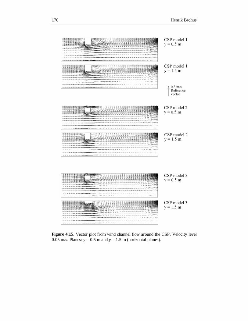
Henrik Brohus170
Figure 4.15. Vector plot from wind channel flow around the CSP. Velocity level0.05 m/s. Planes: y = 0.5 m and y = 1.5 m (horizontal planes).

Chapter 4 Mixing ventilation 171
Figure 4.16. Vector plot from wind channel flow around the CSP. Velocity level0.30 m/s. Planes: y = 0.5 m and y = 1.5 m (horizontal planes).
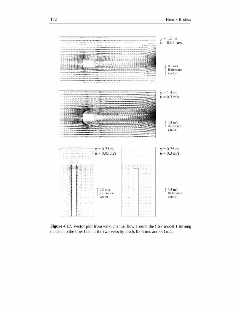
Henrik Brohus172
Figure 4.17. Vector plot from wind channel flow around the CSP model 1 turningthe side to the flow field at the two velocity levels 0.05 m/s and 0.3 m/s.
Chapter 4 Mixing ventilation 173
Inclusion of “head” in CSP model 3 causes a slight deflection of the vertical flowaround the chin, but no major changes of the local field compared with CSPmodel 2 are found. The simulations in Chapter 4.2.4. on personal exposure tocontaminant sources will decide the effect of this possible improvement of thecomputer model of a person.
The purpose of the present simulations and the full-scale measurements in thepreceding chapter is to examine the flow field around a person in a unidirectionalflow field. Therefore, it is important to be aware of the influence of theboundaries on the local uniform flow field around the person, i.e. do the specificsize and construction of the wind channel allow a uniform flow field or do theycause some restrictions in the flow field affecting the generality of the results?
If the vector plots in Figures 4.12. - 4.17. are examined, the geometry of the windchannel does not seem to influence the local flow field around the person in a waythat may affect the personal exposure at the contaminant source locations appliedin this work, which is also the conclusion of smoke visualisations performedduring the experiments.
4.2.4. Simulation of personal exposure
This chapter will present results on personal exposure to a passive pointcontaminant source at different locations relative to the person in theunidirectional flow field, as well as exposure to a planar contaminant source inthe shape of the floor of the wind channel.
Passive point contaminant source
First, some of the transport mechanisms mentioned in the preceding chapter willbe illustrated by means of isoconcentration plots on different characteristicsituations for two different velocity levels, see Figures 4.18. and 4.19.

Henrik Brohus174
Figure 4.18. Dimensionless contaminant concentration distribution in the verticalsymmetry plane (z = 0 m) of the unidirectional flow field created in the windchannel. Velocity level 0.05 m/s. CSP location (x,z) = (0.7,0). Top, left: CSPmodel 1, source location (x,y,z) = (1.2,1.0,0). Top, right: CSP model 3, sourcelocation (x,y,z) = (1.2,1.0,0). Bottom, left: CSP model 1, source location (x,y,z) =(1.2,0.5,0). Bottom, right: CSP model 3, source location (x,y,z) = (1.2,0.5,0). Thecorresponding dimensionless personal exposure, ce
*, is mentioned in the figure.The velocity field is shown in Figure 4.12.
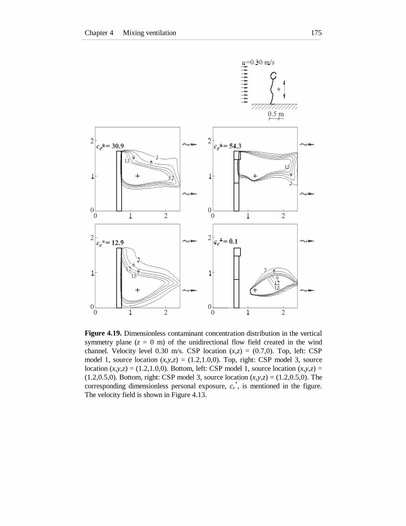
Chapter 4 Mixing ventilation 175
Figure 4.19. Dimensionless contaminant concentration distribution in the verticalsymmetry plane (z = 0 m) of the unidirectional flow field created in the windchannel. Velocity level 0.30 m/s. CSP location (x,z) = (0.7,0). Top, left: CSPmodel 1, source location (x,y,z) = (1.2,1.0,0). Top, right: CSP model 3, sourcelocation (x,y,z) = (1.2,1.0,0). Bottom, left: CSP model 1, source location (x,y,z) =(1.2,0.5,0). Bottom, right: CSP model 3, source location (x,y,z) = (1.2,0.5,0). Thecorresponding dimensionless personal exposure, ce
*, is mentioned in the figure.The velocity field is shown in Figure 4.13.

Henrik Brohus176
Figures 4.18. and 4.19. clearly illustrate many of the characteristics of the twodifferent models of a person mentioned in Chapter 4.2.3., in this case by means ofthe concentration distribution. The significant influence of the velocity level aswell as inclusion of legs is easily seen on the isoconcentration curves and alsovery clearly on the actual personal exposure levels.
The ability of the vortices in the wake region and the human convective boundarylayer in combination to entrain and transport contamination from relative largedistances to the breathing zone is considerable. This applies to both velocity levelsand the two different models of the CSP shown in the two figures. If the exposurelevels are compared with completely mixed conditions, i.e. ce
* = 1, both improved(ce
* = 0) and deteriorated (ce* = 54.3) air quality is found.
In the four figures 4.20. - 4.23. the dimensionless personal exposure is shown as afunction of velocity level and the vertical contaminant source location. The resultsare shown for the three different versions of the Computer Simulated Person. Theexposure measurements made by means of a Breathing Thermal Manikin are alsoincluded to facilitate the comparisons.

Chapter 4 Mixing ventilation 177
Figure 4.20. Dimensionless personal exposure, ce*, of a person standing in a
uniform velocity field as a function of the velocity level and the verticalcontaminant source height above the floor.

Henrik Brohus178
Figure 4.21. Dimensionless personal exposure, ce*, of a person standing in a
uniform velocity field as a function of the velocity level and the verticalcontaminant source height above the floor.

Chapter 4 Mixing ventilation 179
Figure 4.22. Dimensionless personal exposure, ce*, of a person standing in a
uniform velocity field as a function of the velocity level and the verticalcontaminant source height above the floor.

Henrik Brohus180
Figure 4.23. Dimensionless personal exposure, ce*, of a person standing in a
uniform velocity field as a function of the velocity level and the verticalcontaminant source height above the floor. In this case the person is facing theflow field opposite the location in Figures 4.20. - 4.22.
Figure 4.20. shows the exposure in the case of a passive point contaminant sourcelocated 0.7 m behind the person upstream in the unidirectional flow field. Theresults indicate a considerable influence of both velocity level, source location andalso the kind of model used to simulate a person. The variation in thedimensionless exposure level is found to exceed one order of magnitude both incase of simulations and measurements.
When the exposure of the three CSP models is examined, a kind of diagonal isfound in the plots where relatively high exposures occur, starting at a low velocitylevel and a low vertical source location, continuing to a high velocity level and ahigh vertical contaminant source location. In case of the low velocity level theconvective ascending air current along the person is able to transport the

Chapter 4 Mixing ventilation 181
contamination from the lower part of the person to the breathing zone, whereas atthe higher velocities the vortices in the wake region are able to entrain thecontamination and transport it to the breathing zone.
When the source is located at a high level at low velocities the boundary layerflow will protect against exposure, and in case of a low source location at highvelocities the contamination is “washed away”, even though some exposurealways occurs due to the dispersion of the contamination along the route from thesource until the contaminant field reaches the person.
This particular effect is not found to influence the measurements where the BTMis applied, but the exposure levels are found to be of the same order of magnitude,slightly higher than the CSP model 1 and slightly lower than CSP model 2 and 3.
The inclusion of “legs” (CSP model 2 and 3) is seen to influence the results highlyin this case, whereas the inclusion of “head” (CSP model 3) does not alter neitherthe overall flow pattern nor the outline of the exposure isopleths, but in general itseems to increase the exposure level slightly.
Figure 4.21. shows the exposure in the case of a passive point contaminant sourcelocated 0.25 m downstream in front of the person. This case shows some veryhigh levels of exposure. For the measurements the dimensionless exposure, ce
* , isfound to exceed 50 and for the simulations levels above 200 are found.
The vertical source location for the maximum dimensionless exposure is foundbetween 1.0 m and 1.5 m above the floor, i.e. a natural location for a hand-heldcontaminant source. Even at velocity levels required to be in a state of thermalcomfort in typical office environments the exposure levels exceed the “completelymixed conditions” more than 10 times. This fact clearly stresses the importance ofconsidering the local influence of a person located in surroundings whereconcentration gradients prevail.
In Figure 4.22. the horizontal distance between the person and the source ofcontamination is increased from 0.25 m to 0.5 m. Here, the level of exposure isreduced considerably compared with Figure 4.21., which is also expected. Still,however, high dimensionless personal exposure levels are found (exceeding 30 forthe measurements and 60 for the simulations).

Henrik Brohus182
At a low velocity level a protective boundary layer is created in front of theperson in the case of assessments by means of the BTM and CSP models 2 and 3.In this case ce
* = 0 and no exposure takes place.
This particular effect is not caught by CSP model 1 where no “legs” areimplemented. It indicates that the exposure is quite sensitive to the outline of themodels, but it also indicates that even a small change from a standing positionwith the legs assembled to a standing position with the legs slightly spread mayexert an important influence on the exposure in a unidirectional velocity field.
Figure 4.23. shows a simulation of the dimensionless personal exposure where thesource is located 0.25 m in front of the person facing the velocity field. Only CSPmodel 1 and 2 are included. Here, the person is facing the velocity field contraryto the other cases.
For velocity levels above 0.05 m/s - 0.15 m/s the contamination is “washed away”around the person in the case of source locations below 1.0 m This correspondswell with the measurements presented in Figure 4.4. For source locations above1.0 m the dimensionless exposure is almost constant for the different velocitylevels.
It is remarkable that this location causes generally lower exposure levels than theones found in Figure 4.21., where the person facing the contaminant source isturning the back to the flow direction. This is clearly caused by the vorticescreated in the wake region which can be seen, for instance, in Figure 4.15. (Kimand Flynn, 1991b; Brohus and Nielsen, 1995; 1996a).
To illustrate the influence of the direction of the flow field relative to a personholding a contaminant source, three different cases are shown in Figure 4.24.

Chapter 4 Mixing ventilation 183
Figure 4.24. Personal exposure to a hand-held point contaminant source in aunidirectional velocity field of 0.3 m/s. In all cases the contaminant source islocated 1 m above the floor and in a horizontal distance of 0.25 m in front of theCSP model 1. The hatched areas represent contaminant concentrations exceeding10 times the exhaust concentration of the wind channel, i.e. c* ≥ 10. Thedimensionless personal exposure, ce
*, and the personal exposure index, εe, arementioned in the figure for the three different locations relative to the flow field.The source strength and the air flow rate are the same for the three cases.

Henrik Brohus184
Figure 4.24. clearly shows that it may cause an erroneous exposure assessment ifthe personal exposure is calculated solely on the basis of a source strength and anair flow rate. It also suggests the possible benefit that may be obtained if theworker in a spray hood etc. is turning the side to the flow direction instead of theback, both regarding the health effect and also regarding the energy consumptionnecessary to ensure a sufficiently low exposure level.
Planar contaminant source
In the following a planar contaminant source will be applied in the shape of thefloor of the wind channel. The planar source has a constant emission rate.
Figure 4.25. shows some characteristic examples of the concentration distributiongenerated in the wind channel where the entire floor is a contaminant source. Thiskind of source gives a good illustration of the persons ability to entrain andtransport air and thus contaminant from the floor area to the breathing zone.
Again, the influence of the velocity level and the model layout is distinct. Theexposure levels, however, are significantly lower than the previous ones obtainedin the case of a point source located close to the person.
In Figure 4.26. the dimensionless personal exposure is shown as a function of thevelocity level. The exposure of CSP model 2 and 3 is almost similar, and itdecreases when the velocity level increases. CSP model 1 shows a peak in thedimensionless exposure level for 0.15 m/s. This is due to the “assembled legs”and the change from a local flow field dominated by free convection to a localflow field where vortices generated in the wake region play a more and moreimportant role in the contaminant transport processes.

Chapter 4 Mixing ventilation 185
Figure 4.25. Dimensionless contaminant concentration distribution in the verticalsymmetry plane (z = 0 m) of the unidirectional flow field created in the windchannel. The floor (y = 0 m) is a planar contaminant source with a constantemission rate. CSP location (x,z) = (0.7,0). Top, left: CSP model 1, velocity level0.05 m/s. Top, right: CSP model 3, velocity level 0.05 m/s. Bottom, left: CSPmodel 1, velocity level 0.3 m/s. Bottom, right: CSP model 3, velocity level 0.3m/s. The corresponding dimensionless personal exposure, ce
*, is mentioned in thefigure.

Henrik Brohus186
Figure 4.26. Dimensionless personal exposure to a planar contaminant source inthe shape of the floor in the wind channel. The exposure is shown for the threedifferent computational models of a person located at (x,z) = (0.7,0) and for fourvelocity levels 0.05 m/s, 0.15 m/s, 0.30 m/s and 0.45 m/s.
4.2.5. Comparison with exposure models
The results of measurements and computer simulations presented in Chapters4.2.3. and 4.2.4. demonstrate that the personal exposure assessment in the case ofa person exposed to a contaminant source in a unidirectional flow field may berather complex. This fact indicates that there are a number of cases where it isnecessary to apply measurements or computer simulations of the flow field andthe contaminant field if detailed information on the personal exposure is required.
0
1
2
3
0.00 0.15 0.30 0.45
Velocity (m/s)
Exp
osur
e (n
.d.)
CSP model 1CSP model 2CSP model 3

Chapter 4 Mixing ventilation 187
However, in the literature two different exposure models are found on a personstanding in a uniform velocity field exposed to a contaminant source locateddownstream in front of the person. These models are not based on potential flowtheory where the fluid is assumed to be inviscid, like the major part of the existinganalytical models. This is very important in this case, where recirculationobviously plays a significant role. In the subsequent the two models will bedescribed and compared with the results of the present work.
Description of exposure models
The two exposure models described in the following are proposed by George et al.(1990) and further developed by Kim and Flynn (1991a;b).
According to George et al. (1990) the flow around a person standing in a uniformflow field may be compared with the flow around a circular cylinder, see Figure4.27. On that basis a simple conceptual model is developed.
It is assumed that a contaminant source is located close to the person in therecirculation region. The mechanism for contaminant removal from this zone is amixture of turbulent diffusion and vortex shedding (George et al., 1990). Themodel assumes that the person is a two-dimensional circular cylinder, and thatvortex shedding is the principal contaminant removal mechanism.

Henrik Brohus188
Figure 4.27. Visualisation of the flow around a person in a uniform flow field,modelled as a circular cylinder. In part of the wake a Kármán vortex street maybe generated. Reference: Kawamura et al. (1984).
The average steady-state concentration within the recirculation zone is
cS
qstst
st
= (4.2)
where
cst = Average steady-state concentration in recirculation zone (ppm)Sst = Contaminant flow into the recirculation zone (m3/s)qst = Air flow out of the recirculation zone (m3/s)
In order to determine qst, the frequency of vortex shedding, f, has to be known bymeans of the Strouhal number, S

Chapter 4 Mixing ventilation 189
SfD
u= (4.3)
where
S = Strouhal number (n.d.)f = Frequency of vortex shedding (s-1)D = Diameter of object (m)u = Free stream velocity (m/s)
The Strouhal number is a dimensionless group that may be thought of as adimensionless frequency which is a function of the Reynolds number. For a two-dimensional circular cylinder S ≈ 0.21 for Re = 400 - 2⋅105 (Schlichting, 1979).The flow around a person in an office environment or a worker in the industrywill almost always be below Re = 2⋅105 (George et al., 1990), which is alsodemonstrated in Chapter 2.2.2.
The formation region for the vortices is assumed to equal the cylinder diameter,D, and the height of the region is equal to the cylinder height, H. If one-half of thevolume is cleared every time a vortex is shed, the volume contained in one vortex,V, equals
V
DH
=
π
2
2
2
(4.4)
where
V = Volume cleared when a vortex is shed (m3)D = Diameter of cylinder (m)H = Height of cylinder (m)
The frequency, f, determined by the Strouhal number corresponds only to one sideof the cylinder, which gives the total air flow out of the recirculation zone causedby vortex shedding
q fVst = 2 (4.5)
And, finally (George et al, 1990)

Henrik Brohus190
cS
uHDstst=
19
π (4.6)
where D is taken as the width of the chest measured just under the armpits.
Kim and Flynn (1991a) examined the three-dimensional flow around a manikin bymeans of flow visualisation and hot-film anemometry. They found that the regionsubject to vortex shedding ranged only from the chest to the hip, i.e. ∼ 0.3⋅H, andthey found that the average area of one vortex appeared to be 0.7 times the areaof the circle mentioned above. Furthermore, they measured a somewhat lowerStrouhal number, S = 0.19.
If the modifications are implemented in the model the following revised version isobtained (Kim and Flynn, 1991b)
cS
uHDst revisedst
, =50
π (4.7)
Measurements by Kim and Flynn (1991b), using a small-scale, unheated 1 m highmanikin standing in a wind channel with a hand-held point contaminant source,showed that the original model by George et al. (1990) underestimated theaverage concentration in the recirculation region, cst, and that the revised modeloverestimated the concentration. An empirical relation obtained by least squareregression was found both for cst and also for the personal exposure, ce, i.e. (Kimand Flynn, 1991b)
cS
uHDst empiricalst
,
.=
1096 (4.8)
cS
uHDe empiricalst
,
.=
8 62 (4.9)
Apart from the above model George et al. (1990) found an empirical expressionfor the personal exposure as a function of the straight line distance between themouth and the point contaminant source, R. Here, the dimensionless exposure, ce
*,is expressed as a function of the dimensionless distance R/D (George et al., 1990)

Chapter 4 Mixing ventilation 191
( )ce
R D* /.= 695 0135 (4.10)
where
ce* = Dimensionless personal exposure (n.d.)
R = Straight line distance between mouth and contaminant source (m)D = Diameter of object (width of chest) (m)
The empirical expression was found using the above-mentioned small-scalemanikin located in a wind channel. The manikin was exposed to a pointcontaminant source simulated by tracer gas supplied through a ceramic sphere, ø0.64 cm.
Comparison with models
If the empirical expression for the personal exposure to a hand-held pointcontaminant source in a uniform flow field is made dimensionless the followingformula is obtained, where q is the air flow rate (m3/s) of the wind channel
cc
c
S
uHDS
q
q
uHDee
R
st
st
*
..
= = =
8 628 62
(4.11)
The width of the chest for the BTM, the CSP models, and also the cylinder modelof a person mentioned in Chapter 2.2.2. is the same: D = 0.3 m. Inserting theother parameters in equation (4.11) gives
ce* ≈ 50 (4.12)
when the exposure model by Kim and Flynn (1991b) is applied.
In order to make comparisons the small-scale manikin together with thecontaminant source used by Kim and Flynn (1991a;b) and George et al. (1990)must be converted into full scale.

Henrik Brohus192
This results in a source location 1.15 m above the floor. To maintain Reynoldsnumber equality the velocity levels are converted to 0.3 m/s - 0.9 m/s. Thus, thecomparisons should be performed for results in this range.
For the BTM standing in the wind channel with the contaminant source located0.3 m downstream at a height of 1.15 m above the floor, ce
* is found to be 49 and44 for the two velocity levels 0.30 m/s and 0.45 m/s, respectively (see Figure4.10.). This corresponds well with the exposure found by means of the abovemodel in equation (4.10).
Figure 4.28. shows comparisons between the model by George et al. (1990)mentioned in equation (4.10) and measurements using the BTM as well assimulations using CSP model 1 and model 3.
The exposure model mentioned in equation (4.10) and applied in Figure 4.28. isdeveloped for velocity levels ranging from 0.2 m/s to 0.9 m/s when it is convertedto full scale. Furthermore, it has been developed by means of an unheatedmanikin. The results are therefore expected to have the closest correspondence inthe case of the high velocity level. Actually, a rather good correspondencebetween the model and the full-scale measurements using the BTM is found for avelocity level of 0.30 m/s.
For the low velocity level the model overestimates the personal exposure. This ispresumably due to the important effect of the convective boundary layer at thelow velocities which is not considered in this exposure model.
The simulations seem to overestimate the exposure at 0.30 m/s when the source islocated close to the breathing zone.

Chapter 4 Mixing ventilation 193
Figure 4.28. Dimensionless personal exposure, ce*, as a function of the
dimensional straight line distance between the mouth and the point contaminantsource, R/D. R is the distance (m) and D is the chest width (m). The person islocated in the wind channel at (x,z) = (0.7,0). The source is located 1.15 m abovethe floor and at the horizontal distances of 0.30 m, 0.55 m and 0.80 m betweenthe centre of the source and the centre of the person. Two different velocity levels0.05 m/s (top) and 0.30 m/s (bottom) are applied.
u = 0.05 m/s
0
10
20
30
40
0 1 2 3R/D (n.d.)
Exp
osur
e (n
.d.)
BTMCSP model 1CSP model 3George et al., (1990)
u = 0.30 m/s
0
50
100
150
0 1 2 3R/D (n.d.)
Exp
osur
e (n
.d.)
BTMCSP model 1CSP model 3George et al., (1990)

Henrik Brohus194
Both of the above-mentioned exposure models are shown to correspond well withthe present full-scale measurements when they are used in their range ofapplication. However, for different source locations and lower velocities theyshould not be used. This is clearly seen in Figure 4.28. and is also illustrated fromthe fact that equation (4.9) leads to a statement of ce
* ≈ 50, i.e. no variation withrespect to source location or velocity level which was found to be highlysignificant in the preceding chapters.
The range of application for the present measurements and simulations, togetherwith some other limitations will be discussed in Chapter 5.
4.3. Mixing ventilated room
In the previous Chapter 4.2. personal exposure assessment in the case of mixingventilation was examined by looking at a part of the flow field in a room. Thelocal flow field was assumed to be unidirectional, see Figure 4.1., and a windchannel was applied in order to generate the flow. This chapter presents CFDsimulations on personal exposure to contaminant sources located in a mixingventilated room where the entire flow field in a mixing ventilated room isincluded.
4.3.1. Geometry and boundary conditions
It is chosen to perform the simulations on a well documented test case in order tofacilitate comparisons between the present simulations and the measurements andsimulations found in the literature. The test case is described by Nielsen (1990),and it has been used as part of the International Energy Agency, Annex 20 work.
The mixing ventilated room is shown in Figure 4.29. where the co-ordinate systemis defined and the dimensions are mentioned.
Like the previous CFD simulations only one half of the symmetric room issimulated (z ≥ 0 m). Three different cases are examined: an empty room and twodifferent locations of the Computer Simulated Person (CSP) model 1 as shown inFigure 4.30.

Chapter 4 Mixing ventilation 195
Figure 4.29. Geometry of the mixing ventilated room applied in the CFDsimulation. The air is supplied by the inlet (1) located close to the ceiling, and theair is exhausted by the return opening (2) located close to the floor in the oppositeend. The CSP model 1 (3) is located in the symmetry plane, z = 0 m.
The inlet conditions for the test case are prescribed according to Nielsen (1990),for instance, the inlet velocity is 0.455 m/s which correspond to an air change rateof 10 h-1. The supply air temperature is 21°C. In Case 1 the flow is isothermal,and in Case 2 and Case 3 the only heat source is the CSP with a surface heat fluxof 25 W/m2. The walls are adiabatic and surface friction is included by means ofwall functions (see Chapter 2.3.2.3.). The grid size is summarised in Table 4.3..
Table 4.3. Number of cells applied in simulation of the mixing ventilated room.Case Cells in direction Total
x y z1
2, 36375
3548
1821
39,69075,600

Henrik Brohus196
Figure 4.30. In the CFD simulations only one half of the symmetric room issimulated, z ≥ 0 m. Three different cases are examined, Case 1: empty room,Case 2: CSP model 1 located at (x,z) = (3,0), and Case 3: CSP model 1 located at(x,z) = (6,0).
4.3.2. Simulation of the flow field
In Figures 4.31., 4.32. and 4.33. the flow field of the mixing ventilated room isshown by means of vector plots for the three different cases.

Chapter 4 Mixing ventilation 197
Figure 4.31. Vector plot from mixing ventilated room Case 1, 2 and 3. Plane z =0 m (vertical symmetry plane). See also Figure 4.30.
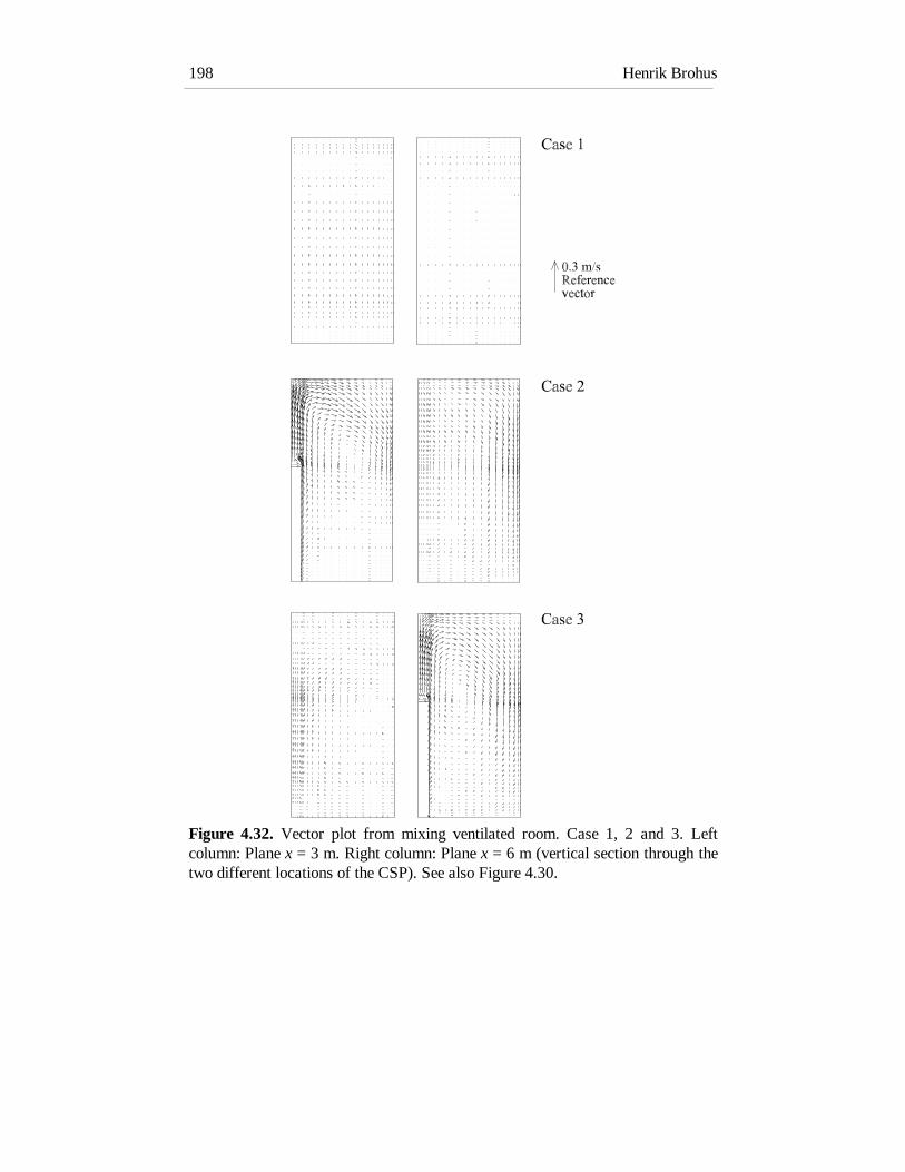
Henrik Brohus198
Figure 4.32. Vector plot from mixing ventilated room. Case 1, 2 and 3. Leftcolumn: Plane x = 3 m. Right column: Plane x = 6 m (vertical section through thetwo different locations of the CSP). See also Figure 4.30.

Chapter 4 Mixing ventilation 199
Figure 4.33. Vector plot from mixing ventilated room Case 1, 2 and 3. For eachcase the two horizontal planes are shown: y = 1.5 m (breathing zone height) and y= 2. 9 m (0.1 m below the ceiling). See also Figure 4.30.

Henrik Brohus200
The flow field in the empty mixing ventilated room (Case 1) shows a typicalrecirculating flow field. The flow is found to be unidirectional in the major part ofthe room, even though the direction changes sign from the upper part of the roomto the lower part. The exhaust is seen to exert only a small and local influence onthe general field, whereas the inlet is decisive in combination with the boundaryconditions. If the three figures 4.31., 4.32. and 4.33. are observed with respect tothe empty room an almost two-dimensional flow is seen and only in Figure 4.33.minor parts if the field are found to be three-dimensional.
When a person in the shape of a CSP is located in the room (Case 2 and Case 3)the flow field is significantly affected both in general and, especially, close to theperson where the local Archimedes number is high. The plume above the person isdistinct and only close to the ceiling it is possible for the supply air jet and theceiling to entrain and deflect it, see Figure 4.31.
In Figure 4.32. which shows vertical sections through the different locations ofthe person a local recirculating flow is generated perpendicular to the main flowdirection. A strong three-dimensional effect of the CSP is also clearly seen inFigure 4.33. close to the ceiling.
In the breathing zone height the velocity level is increased in Case 2 and Case 3compared with the empty room. The explanation on the increased velocity levelmay be found in a combination of a redistribution of the momentum from the inletdevice and also from a supply of momentum from the plume created by the heatedCSP.
If the flow field close to the CSP is examined in both Case 2 and Case 3, it isfound to approach the uniform flow field in the wind channel well, for instance,the important recirculating vortices in the wake region are clearly recreated in thiscase, see Figure 4.33. The velocity level obtained around the CSP in the mixingventilated room is approximately 0.05 m/s.
Figures 4.34. and 4.35. show comparisons between measurements by Nielsen(1990) and the present simulations regarding a vertical velocity profile at twodifferent locations in the ventilated room.

Chapter 4 Mixing ventilation 201
Figure 4.34. Vertical velocity profiles in the mixing ventilated room at (x,z) =(3,0) in Case 1, 2 and 3 compared with measurements from Nielsen (1990).
0
1
2
3
-0.2 0.0 0.2 0.4Velocity (m/s)
Hei
ght (
m)
Case 1Case 2Case 3Nielsen (1990)

Henrik Brohus202
Figure 4.35. Vertical velocity profiles in the mixing ventilated room at (x,z) =(6,0) in Case 1, 2 and 3 compared with measurements from Nielsen (1990).
If the velocity profiles obtained at the simulation of the empty room (Case 1) arecompared with the measurements a reasonable correspondence is found, bothregarding the peak levels and the profile shape. As it was also seen on the vector
0
1
2
3
-0.2 0.0 0.2 0.4Velocity (m/s)
Hei
ght (
m)
Case 1Case 2Case 3Nielsen (1990)

Chapter 4 Mixing ventilation 203
plots the velocity field is significantly influenced by the presence of the CSP. Thisfact results in a decreased maximum velocity close to the ceiling, especiallypronounced in Figure 4.35. where the distance between the inlet opening and theprofile location is high. A local increase in the velocity level in the occupied zoneis found in Case 3, Figure 4.34.
4.3.3. Simulation of personal exposure
This chapter will present simulations of personal exposure to point sources atdifferent locations in the mixing ventilated room as well as a planar source in theshape of the floor. The simulations are performed for the empty room and twodifferent locations of the CSP.
Passive point contaminant source
The point source is the same one as applied in the case of displacement ventilationand of flow in the wind channel.
In order to examine how the contaminant source and the CSP interact with thegeneral flow in the mixing ventilated room the source is located at a higherhorizontal distance than in the previous simulations on the wind channel.
In Figure 4.36. and Figure 4.37. isoconcentration plots are shown for twodifferent locations of the contaminant source relative to the person in Case 2 andCase 3, respectively.
If the room air is assumed to be completely mixed, the dimensionless contaminantconcentration as well as the personal exposure will equal 1 in all cases shown inFigure 4.36. and Figure 4.37. This is due to the fact that the air flow rate and thesource strength are the same in the different situations. However, the simulationsclearly show the significant concentration gradients generated close to thecontaminant sources and also close to the CSP in two of the plots.
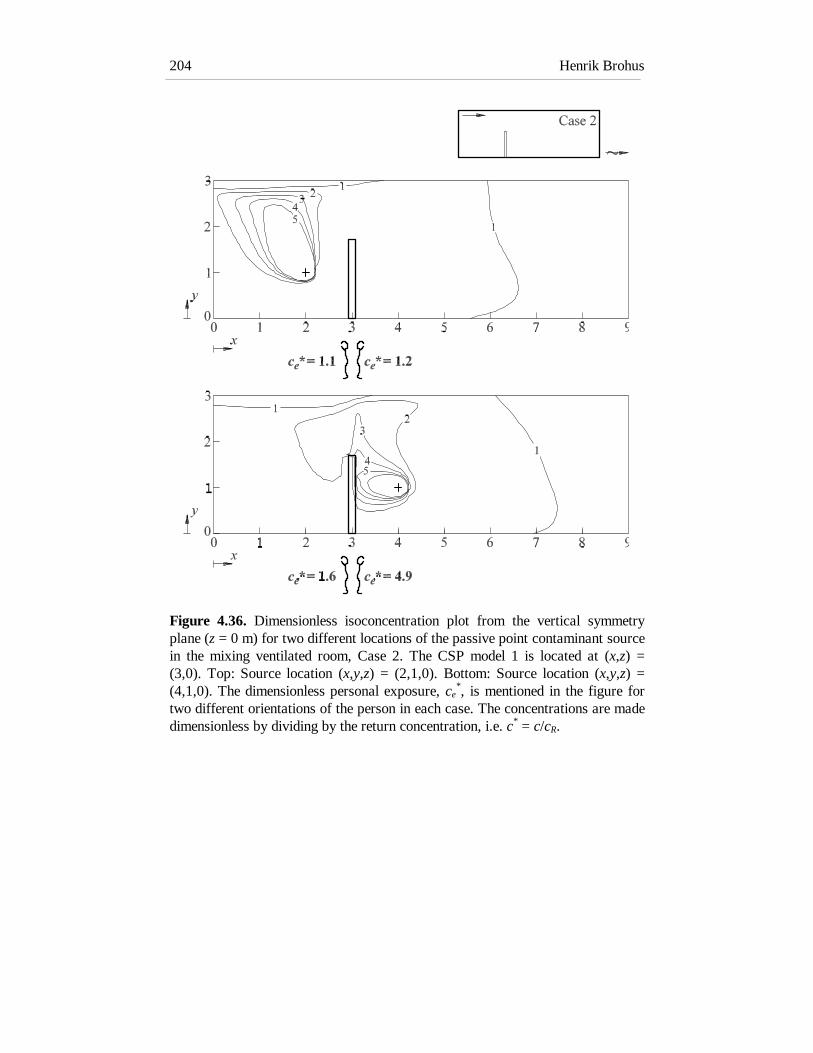
Henrik Brohus204
Figure 4.36. Dimensionless isoconcentration plot from the vertical symmetryplane (z = 0 m) for two different locations of the passive point contaminant sourcein the mixing ventilated room, Case 2. The CSP model 1 is located at (x,z) =(3,0). Top: Source location (x,y,z) = (2,1,0). Bottom: Source location (x,y,z) =(4,1,0). The dimensionless personal exposure, ce
*, is mentioned in the figure fortwo different orientations of the person in each case. The concentrations are madedimensionless by dividing by the return concentration, i.e. c* = c/cR.

Chapter 4 Mixing ventilation 205
Figure 4.37. Dimensionless isoconcentration plot from the vertical symmetryplane (z = 0 m) for two different locations of the passive point contaminant sourcein the mixing ventilated room, Case 3. The CSP model 1 is located at (x,z) =(6,0). Top: Source location (x,y,z) = (5,1,0). Bottom: Source location (x,y,z) =(7,1,0). The dimensionless personal exposure, ce
*, is mentioned in the figure fortwo different orientations of the person in each case. The concentrations are madedimensionless by dividing by the return concentration, i.e. c* = c/cR.

Henrik Brohus206
The concentration gradients result in a dimensionless exposure ranging form 1.1to 4.9, highly dependent on source location and CSP location. Furthermore,different orientations of the CSP, for a fixed location, manage to change theexposure from 1.6 to 4.9 in Figure 4.36.
A dimensionless personal exposure of 4.9 is an exposure approximately five timesas high as found in the exhaust air. This corresponds to a personal exposure indexof εe = 0.2. Even higher exposure levels may be obtained if the source is locatedcloser to the person as shown in Chapter 4.2.4.
The three figures 4.38., 4.39. and 4.40. show the personal exposure as a functionof contaminant source location in the vertical symmetry plane (z = 0 m) of themixing ventilated room in Case 1, 2 and 3, respectively.
The results in Figures 4.38., 4.39. and 4.40. show the exposure as a function ofthe location of the passive point contaminant source. For source locations in theoccupied zone it is found that the dimensionless personal exposure often exceeds2. Very high levels may be obtained when the source is found close to the person.
At a certain location of the person, the exposure level may be significantlyaffected if the person is turned around. In all cases the dimensionless exposurelevels are found to exceed 1, i.e. ce
* ≥ 1, resulting in a personal exposure index εe
≤ 1. This result is quite contrary to displacement ventilation where εe ≥ 1, seeChapter 3.
The local influence of a person in a ventilated room with concentration gradientsmay be examined if the empty room in Figure 4.38. is compared with thesimulations including a person as shown in Figures 4.39. and 4.40. Here, it isdemonstrated that the personal exposure may deviate considerably from theconcentration at the same location, but without the local impact of a person, i.e.εP ≠ εe .
This obviously stresses the importance of including the local influence of a personwhen the exposure is assessed. It is not sufficient to know the local concentrationlevel of an empty room, the local impact of the person is distinct and should beconsidered in the exposure assessment.

Chapter 4 Mixing ventilation 207
Figure 4.38. Dimensionless concentration at the breathing zone location, cP*, as a
function of point contaminant source location in the empty vertical symmetryplane (z = 0 m) of the mixing ventilated room, Case 1. Top: Dimensionlessconcentration at (x,y,z) = (3,1.5,0). Bottom: Dimensionless concentration at(x,y,z) = (6,1.5,0). The concentrations are made dimensionless by dividing by thereturn concentration, i.e. cP
* = cP/cR.

Henrik Brohus208
Figure 4.39. Dimensionless personal exposure, ce*, as a function of point
contaminant source location in the vertical symmetry plane (z = 0 m) of themixing ventilated room, Case 2. The results are shown for two differentorientations of the CSP model 1, located at (x,z) = (3,0). The personal exposure ismade dimensionless by dividing by the return concentration, i.e. ce
* = ce/cR.
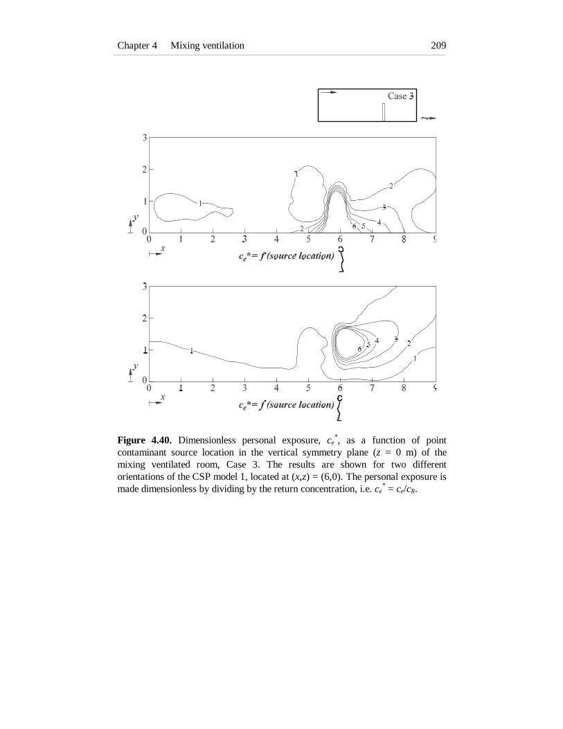
Chapter 4 Mixing ventilation 209
Figure 4.40. Dimensionless personal exposure, ce*, as a function of point
contaminant source location in the vertical symmetry plane (z = 0 m) of themixing ventilated room, Case 3. The results are shown for two differentorientations of the CSP model 1, located at (x,z) = (6,0). The personal exposure ismade dimensionless by dividing by the return concentration, i.e. ce
* = ce/cR.

Henrik Brohus210
Figure 4.41. Dimensionless concentration in the vertical symmetry plane (z = 0m). The floor is a planar source. The dimensionless personal exposure, ce
* (cP* in
Case 1) is mentioned for the different orientations of the CSP model 1.

Chapter 4 Mixing ventilation 211
Planar contaminant source
Figure 4.41. shows the concentration distribution in the mixing ventilated room inthe case of a constantly emitting planar contaminant source in the shape of thefloor.
The concentration distribution in Figure 4.41. for Case 1 is also simulated byNielsen (1981) using a two-dimensional CFD calculation, and a very goodagreement is found.
It is seen how the concentration level increases towards the lower left part of theroom and how the CSP modifies the distribution for the two different locations.
When the exposure levels are compared an important influence of location andorientation of the person are found again. Furthermore, it is found that cP
* ≠ ce*.
In Case 3 an example of a dimensionless exposure below 1 is found, i.e. improvedair quality compared with “completely mixed conditions”.
4.4. Conclusion
In this chapter personal exposure to contaminant sources in a mixing ventilatedroom is examined.
The unidirectional flow field generated in a wind channel is assumed to representthe local flow field around a person in a mixing ventilated room.
Full-scale wind channel measurements using the Breathing Thermal Manikin(BTM) are performed as well as CFD simulations using the three differentversions of the Computer Simulated Person (CSP). The CSP is also applied in asimulation including the whole flow field in a mixing ventilated room.
The contaminant distribution is generated by a passive contaminant source. Forthe computer simulations a planar source is also applied in the shape of the floorin the wind channel and in the mixing ventilated room.
It is found that the personal exposure to a contaminant source in a unidirectionalflow field depends highly on the source location as well as the flow direction
Henrik Brohus212
relative to the person. The uniform velocity level is also a very important factor toconsider.The vortices generated in the wake in front of a person turning the back to theflow direction have a considerable ability to entrain contamination. Thecontamination is transported to the breathing zone where is causes exposure. Thevortices are found to entrain contamination from a horizontal distance exceeding0.5 m.
Personal exposure levels in the wind channel for a typical hand-held source arefound to be more than 50 times higher than the exhaust concentration for themeasurements, and even higher levels are obtained for the simulations. Thismeans that the actual exposure in this case is 50 times higher than it would be ifthe exposure was assessed by an assumption of fully mixing. This effect is alsoseen in the computer simulations of the mixing ventilated room.
The measurements in the wind channel by means of the BTM are found tocorrespond well to results from the literature.
Personal exposure assessed by the CSP deviates somewhat from the exposureassessed by the BTM. However, the results are of the same order of magnitudeand the CSP is capable of simulating all the important phenomena observed closeto a person. Inclusion of “legs” in the CSP is found to affect the exposureconsiderably, especially when the contaminant source is located close to the floor.

Chapter 5 General discussion and conclusion 213
Chapter 5
General discussion and conclusion
This chapter will summarise and discuss the results presented in the thesisregarding the tools for personal exposure assessment, the displacement ventilationcase and the mixing ventilation case. Furthermore, some limitations are discussedand, finally, a number of future perspectives will be outlined.
Purpose
In Chapter 1 it is stated that many people spend more than 90% of their time in amore or less artificial indoor environment. This indoor environment is oftensubject to contaminant sources both in the case of residential buildings, officesand occupational buildings. This stresses the importance of a proper exposureassessment.
Usually, the exposure models treat the indoor environment as well-mixedcompartments without concentration gradients. However, in practice gradientswill prevail, for instance, close to the contaminant sources or in the case ofdisplacement ventilation where the concentration gradients are utilised to improvethe ventilation effectiveness.
When gradients prevail in a ventilated room the presence of a person may modifythe concentration field locally due to the influence of e.g.:
- excess surface temperature
- obstacle to the flow field
- movements, etc.

Henrik Brohus214
The local influence on the flow field and concentration field may affect thepersonal exposure significantly. This raises the need for improved exposuremodels where concentration gradients and the influence of a person areconsidered.
Tools for personal exposure assessment
Three different tools for personal exposure assessment are presented in Chapter 2together with the theoretical basis:
1. A Breathing Thermal Manikin which is a heated full-scale model of a womanequipped with an artificial lung to simulate respiration. Tracer gas is used tosimulate contamination.
2. A Computer Simulated Person which is a numerical model of a person appliedin Computational Fluid Dynamics where the flow field and the contaminanttransport are simulated.
3. A Trained Sensory Panel which is a group of persons trained to judge the airquality in comparison with references with known levels of perceived air quality.
The three tools are all able to consider the local influence of persons in ventilatedrooms where concentration gradients prevail.
The tools are applied on the two major room ventilation principles, namely thedisplacement principle and the mixing principle. This is done both in order toexamine the tools on different test cases, but also to investigate how the exposureassessment is influenced when concentration gradients and the local effect of aperson are considered.
The Breathing Thermal Manikin (BTM) and the Trained Sensory Panel (TSP) aremost suitable for laboratory and field investigations where the main purpose isresearch and development of exposure models, etc. The Computer SimulatedPerson (CSP) may also be used for practical engineering purposes due to therelatively simple geometry.
The BTM is very suitable in steady-state (mid term and log term) exposuremeasurements where tracer gas is used to simulate contaminant dispersion. Due tothe artificial lung the concentration of inhaled air is easily found.

Chapter 5 General discussion and conclusion 215
If movements have to be considered they may be simulated by locating the BTMin a unidirectional flow of a wind channel, or it may be necessary to replace theBTM with a real person equipped with a sampling device.
The TSP may of course be applied to assess the perceived air quality, but it canalso be used to assess the contaminant concentration of inhaled air where therelation between concentration and perceived air quality is known for a tracer gas.This is the case for the reference gas 2-propanone. However, the TSP is limited to(very) short-term exposure assessment in order to avoid adaptation. This implies,strictly speaking, that only the first inhalation of contaminated air may beassessed properly by the TSP.
If the CSP is applied for exposure assessment it is necessary to have a certainamount of experience in using Computational Fluid Dynamics in order toprescribe a proper set of boundary conditions etc. which are decisive for theresult. Using the CSP it is possible to simulate transient behaviour, too, eventhough it is quite time-consuming and limited to a relatively short time span inpractice.
One limitation of the three tools for personal exposure in this thesis is the fact thatthey are used only to assess personal exposure to gaseous contaminants or smallerparticles acting like a gas. However, both the BTM and the CSP may be extendedto assess exposure to for instance dust particles. It requires new measuringequipment to analyse the contents of the inhaled air and a modification of theconcentration equation governing the contaminant transport, respectively.
Measurements made by using the BTM standing in the wind channel are found tocorrespond well with results from the literature.
The exposure assessed by means of the CSP deviates somewhat from theexposure assessed by the BTM. However, the results are of the same order ofmagnitude and the CSP is capable of simulating the important phenomenaobserved close to a person. Inclusion of “legs” in the CSP is found to affect theexposure considerably, especially for contaminant sources which are located closeto the floor. Some possible improvements of the CSP are mentioned in thesubsequent.
Henrik Brohus216
New quantities
Two new quantities are defined.
A new ventilation effectiveness: the personal exposure index, εe, see equation(1.4). The personal exposure index expresses the effectiveness actuallyexperienced by a person in a ventilated room.
The other new quantity is: the effectiveness of entrainment in the human boundarylayer, ηe, see equation (3.1). ηe expresses the ability to supply (fresh) air from thefloor area to the breathing zone. It is mainly used in connection with displacementventilation and applied in an exposure model for displacement ventilation.
Both of the new quantities result from considering the local impact of persons onthe personal exposure. Results from full-scale measurements and computersimulations demonstrate their applicability in expressing the difference betweenthe air quality actually experienced and the mean air quality in the occupied zoneor in the breathing zone height at a “neutral” place.
Displacement ventilation
Personal exposure in rooms ventilated after the displacement principle isexamined by means of full-scale measurements in two different test rooms andcomputer simulations of the flow in one of the rooms.
The contaminant distribution in the measurements is generated by point sources.Non-passive (warm) sources are applied to generate the characteristic two-zonalconcentration distribution with a separation in a cleaner, lower zone and an upper,more contaminated zone in the displacement ventilated room. Upward pointingtubes located above heat sources supply the contamination (N2O or 2-propanone).A passive (cold) source is applied in order to investigate the influence ofcontaminant sources located close to persons. This contaminant source comprisesa neutral density mixture of N2O and He supplied through a porous foam rubberball. In the CFD simulations a planar source is applied in the shape of aconstantly emitting floor, apart from the above-mentioned sources.

Chapter 5 General discussion and conclusion 217
It is found that the stratified flow and the considerable concentration gradients ina displacement ventilated room necessitate an improvement of the widely usedcompartmental approach, where the room air is assumed to be fully mixed.
The flow in the human boundary layer is able, to a great extent, to entrain airfrom below the breathing zone, thus improving the quality of the inhaled air incase of non-passive contaminant sources.
The air quality experienced by the occupants in the displacement ventilated roomis significantly improved compared with mixing ventilation. The improved airquality is both found by means of steady-state chemical measurements andsensory measurements where the TSP judges the perceived air quality.
Movements cause the air quality to decrease due to the disturbance of the humanboundary layer which promotes the high air quality.
A personal exposure model for displacement ventilated rooms is proposed. Themodel takes the concentration gradient and the influence of the human thermalboundary layer into account. It is based on the present full-scale measurementstogether with measurements from various references. The model is easy-to-useand suitable for the design of displacement ventilation systems in practice. It islimited to cases where the characteristic two-zonal flow prevail, and to caseswithout considerable movements of the persons.
Entrainment of air in the human boundary layer is usually an advantage but theresults show also the possible disadvantage when passive contaminant sources arepresent. In this case the convective current around the person may transportcontaminated air to the breathing zone, giving rise to increased exposure. Poorsystem performance is found in the case of a passive contaminant released in thelower part of the room close to the occupant.

Henrik Brohus218
Mixing ventilation
Exposure assessment in a mixing ventilated room is examined by means ofmeasurements and simulations of the unidirectional flow around a person standingin a wind channel as well as by simulations of the entire flow field in a mixingventilated room.
The unidirectional flow field generated in the wind channel is assumed torepresent the local flow field around a person in a mixing ventilated room.
Here, the contaminant distribution is generated by a passive point contaminantsource. For the computer simulations a planar source is also applied in the shapeof the floor in the wind channel and in the mixing ventilated room.
The personal exposure to a contaminant source in the unidirectional flow field isfound to depend highly on both the source location and the flow direction relativeto the person. The uniform velocity level is also found to be an important factor toconsider.
Vortices generated in the wake in front of a person turning the back to the flowdirection have a considerable ability to entrain contamination. The contaminationis transported to the breathing zone where is causes exposure. The vortices arefound to entrain contamination from a horizontal distance exceeding 0.5 m.
Personal exposure measured by means of the BTM standing in the wind channelwith a typical hand-held source is found to be more than 50 times higher than theexhaust concentration, and even higher levels are obtained for the correspondingcomputer simulations. This effect is also seen in the computer simulations of themixing ventilated room.
The findings clearly stress the need of an improved exposure assessment in caseswhere the contaminant source is located in the vicinity of persons.
The computer simulations of the mixing ventilated room reveal that theconcentration of inhaled contaminant may easily be twice as high as the returnconcentration, even though the contaminant source is located at some distancefrom the person depending on the flow direction relative to the person and thecontaminant source.

Chapter 5 General discussion and conclusion 219
The simulations show also that it is not sufficient to know the local concentrationlevel of an empty room, the local impact of a person is distinct and should beconsidered in the exposure assessment.
Limitations
Apart from the limitations that are already mentioned a number of other thingsmay be useful to acknowledge.
Only the personal exposure to gaseous contaminants by means of respiration isconsidered in the thesis. Exposure to larger particles, dust, fibres or gaseouscontaminants with a density deviating considerably from the room air may alsocause a substantial health risk and discomfort and should of course be consideredwhen it occurs.
Transient behaviour with considerable movements takes place when the TSP isjudging the perceived air quality, and some results from the wind channel casemay also simulate movements and quasi transient conditions. Most of the results,however, arise from steady-state conditions. Therefore, they are mainly applicablefor mid-term and long-term exposure assessment in cases where only slightmovements occur.
Future perspectives
The author foresees that the development of more advanced personal exposuremodels will continue with a growing rate in the future. At the same time there willpresumably be a growing need for relatively simple models which may be appliedfor practical engineering design purposes.
The models may be developed both in a direction where the local impact of aperson is stronger implemented, but also in a direction where advanced statisticalmethods are applied in order to take into account the transient behaviour,movements and the various activities performed in a ventilated enclosure wherecontaminant sources prevail.
The tools for personal exposure assessment presented in this thesis may beimproved in different ways. The Computer Simulated Person can be improved by

Henrik Brohus220
using a rounded geometry and a low-Reynolds number turbulence model. Theboundary conditions in the CFD simulations can also be modified in order tosimulate the full-scale measurements better together with a revised grid layoutaround heat and contaminant sources and at locations where steep gradientsoccur. Transient behaviour can also be included in the computer calculations.
An obvious new element in the “tool box” may be measurements by means of realpeople wearing personal exposure monitors. In that way it is possible to considerthe transient behaviour and compare with the results and models made understeady-state conditions for validation and further progress.
An other future perspective is the consideration of particles, fibres, and gaseouscontaminants with a density deviating from the surrounding room air. Regardingparticles etc. the exposure models may also be expanded to “dose models” where,for instance, particle deposition in the upper airways is calculated.
Appendix A Heat balance for a person 221
Appendix A
Heat balance for a person
In order to describe how the Breathing Thermal Manikin is controlled, it isnecessary to derive a relationship between the skin temperature and the sensibleheat loss. To achieve this relationship a total heat balance for the human body isset up.
A.1. Steady-state total heat balance for a person
During steady-state conditions the metabolic heat production, M, will normally bealmost equal to the total heat loss of a person, Qm, i.e. the energy flow due touseful, external mechanical work is assumed to be insignificant.
Q M Q Qm sk res= = + (A.1)
where
Qm = Total heat loss from person (W/m2)M = Metabolic heat production (W/m2)Qsk = Heat loss from skin surface (W/m2)Qres = Heat loss by respiration (W/m2)
The heat loss from the skin and the respiration may be expressed as
Q Q Esk t s= + (A.2)
and, if heat transfer by conduction is assumed to be very small
Q R Ct = + (A.3)
where

Henrik Brohus222
Qt = Sensible heat loss (W/m2)Es = Latent heat loss (W/m2)R = Radiative heat loss (W/m2)C = Convective heat loss (W/m2)
Thus
Q Q Q Et m res s= − − (A.4)
A.2. Heat loss by respiration
The heat loss by respiration, Qres, consists of a convective part, Cres, and anevaporative part, Eres.
Q C Eres res res= + (A.5)
Here,
( )C m c t t Ares res p ex a Du= −�
/ (A.6)
where the pulmonary ventilation rate (kg/s) may be expressed as (Fanger, 1972)
� .m K M Mres res= = ⋅ −2 58 10 6 (A.7)
and cp is the specific heat of the ambient air (J/kg°C), tex is the temperature ofexhaled air (°C), ta is the temperature of ambient air (°C) and, finally, ADu is theDuBois area (body surface area in m2).
The temperature of exhaled air can be expressed as a function of the ambienttemperature and the humidity ratio of inhaled air (kg H2O/kg air) (ASHRAE,1993). If tex is evaluated under standard conditions (20°C, 50% rh, sea level), weget an exhaled air temperature of 34°C, and thus
( )C M tres a= ⋅ −−1 10 343.43 (A.8)

Appendix A Heat balance for a person 223
The evaporative part of the respiratory heat loss, Eres, can be found as
( )E m h W W Ares res fg ex a Du= −� / (A.9)
where
hfg = Heat of vaporisation of water (e.g. 2.43⋅106 J/kg)Wex = Humidity ratio of exhaled air (kg H2O/ kg air)Wa = Humidity ratio of inhaled (ambient) air (kg H2O/ kg air)
Here, Wa may be expressed as a function of the water vapour pressure in theambient air, pa, and the barometric pressure. If the proper numbers aresubstituted, we obtain the relation
( )E M pres a= ⋅ −−1 73 10 58343. (A.10)
where
pa = Water vapour pressure in the ambient air (Pa).
A.3. Latent heat loss
The latent heat loss may be divided into diffusion through the skin, Ed, andsweating, Esw
( )E h m p pd fg p sk s a= −, (A.11)
where
mp,sk = Permeance coefficient of the skin (1.271⋅10-9 kg/(m2 s Pa) )ps = Saturated water vapour pressure at skin temperature (Pa)
The saturated water vapour pressure may be expressed as a function of the skintemperature, ts.
p ts s= −256 3373 (A.12)
Henrik Brohus224
Fanger (1972) found a relationship between the skin temperature and the heatproduction, which is necessary to achieve a state of thermal comfort
t Ms = +35 7 0 028. . (A.13)
If ts is inserted in the expression for ps and this is applied in the equation for Ed,we obtain the latent heat loss by diffusion through the skin
( )E M pd a= ⋅ − −−3 09 10 5765 7173. . (A.14)
Fanger (1972) also found a relationship between Esw and M which is necessary toobtaining thermal comfort
( )E Msw = −0 5815.42 . (A.15)
A.4. Skin temperature vs. sensible heat loss
By means of the above expressions it is possible to derive the relationshipbetween the skin temperature and the sensible heat loss. We assume, as mentionedpreviously, that the total heat loss equals the metabolic heat production, i.e. Qm =M.
To “eliminate” the latent heat in the total heat balance we assume in the equationsfor Qres and Es, as a reasonable approximation, that the water vapour pressure inthe ambient air is 1500 Pa corresponding to an air temperature of 24°C and arelative humidity of 50% which is equivalent to typical indoor conditions (Tanabeet al., 1994).
( )Q Q Qres m m= ⋅ − + ⋅ −− −143 10 34 24 173 10 5834 15003 5. . ( ) (A.16)
Q Qres m= 0 0893. (A.17)

Appendix A Heat balance for a person 225
( ) ( )E Q Qs m m= ⋅ − − + −−309 10 5765 717 1500 0 42 58153. . . . (A.18)
E Qs m= −03978 112441. . (A.19)
If the two equations are inserted in the total heat balance, we get
Q Qm t= −195 2192. . (A.20)
This equation may be inserted in Fanger´s (1972) thermal comfort relationshipbetween the skin temperature and the total heat loss (the metabolic heatproduction)
( )t Q Qs m t= − = − −35 77 0 0275 35 77 0 0275 195 21 92. . . . . .
(A.21)
and, finally
t Qs t= −36 0 054.4 . (A.22)
A.5. Surface temp. vs. insulation value of clothing
The above formula expresses the skin temperature as a function of the sensibleheat loss (i.e. radiative and convective heat loss). Often, however, it is the surfacetemperature of a person that is needed, for instance, when making calculationsregarding the natural convective boundary layer etc. The surface temperature of aperson will deviate from the skin temperature when s/he is clothed.
In the following an expression of the surface temperature (i.e. the temperature ofthe clothing),tcl, as a function of the skin temperature, ts, and the insulation valueof the clothing, Icl, is derived.
The sensitive heat flux through the clothing may be expressed as
Qt
R
t t
Rtcl
s cl
cl
= =−∆
(A.23)

Henrik Brohus226
where ∆t is the temperature difference between the skin and the surfacetemperature of the clothing, and Rcl (m2°C/W) is the thermal resistance againstheat loss. When 1 clo = 0.155 m2°C/W the thermal resistance, Rcl, in SI-unitsbecomes
R Icl cl= 0155. (A.24)
where Icl is the clothing insulation (in clo). When ts is expressed as a function ofQt and the equation above is used, we get
Qt
ts=
−36 4
0 054
.
. (A.25)
and thus
t t Q I tt
Icl s t cl ss
cl= − ⋅ = −−
⋅0155
36 4
0 0540155.
.
.. (A.26)
t t I Icl s cl cl= + ⋅
−
⋅⋅1
0155
0 054
36 4 0155
0 054
.
.
. .
. (A.27)
If the skin temperature is known and the clothing insulation it is possible to findthe surface temperature of the person, tcl.
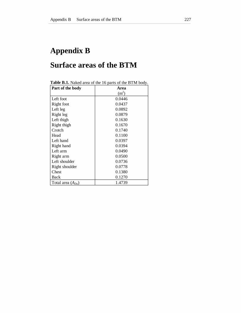
Appendix B Surface areas of the BTM 227
Appendix B
Surface areas of the BTM
Table B.1. Naked area of the 16 parts of the BTM body.Part of the body Area
(m2)Left footRight footLeft legRight legLeft thighRight thighCrotchHeadLeft handRight handLeft armRight armLeft shoulderRight shoulderChestBack
0.04460.04370.08920.08790.16300.16700.17400.11000.03970.03940.04900.05000.07360.07780.13800.1270
Total area (ADu) 1.4739

Henrik Brohus228
Appendix C Measurement of the convective heat transfer coefficient 229
Appendix C
Measurement of the convective heattransfer coefficient
To validate the performance of the Breathing Thermal Manikin (BTM) theconvective heat transfer coefficient, hc, is measured and compared with resultsfound in the literature.
C.1. Measurement set-up
The measurements are performed in a displacement ventilated room with a smallair change rate and a small vertical temperature gradient.
The dimensions of the room are 8 m x 6 m x 4.5 m (length x width x height). Theair flow rate is 0.040 m3/s corresponding to an air change rate of 0.67 h-1. Heatload is generated by two person simulators (2 x 100 W) and a point heat source(500 W), apart from the manikin itself. The manikin has a surface area of ADu =1.4739 m2. In the present measurements it is naked (Icl = 0 clo).
The manikin is suspended from the ceiling so that the feet are raised 0.3 m abovethe floor to avoid conduction and the relatively high velocities at the floor. In thatway the velocity in the surroundings around the manikin is less than 0.05 m/s.Therefore, it is concluded that the flow around the body is free convection(Chapter 2.2.2.2.).
The air temperature and the surface temperature of the surrounding walls, ceilingand floor are measured together with the skin temperature and the total sensibleheat loss from the BTM (radiation and convection).
Two cases are examined corresponding to slightly different temperatures of thesurroundings. In Table C.1. some of the results from the measurements arepresented.

Henrik Brohus230
Table C.1. Measurement results from Case 1 and Case 2 used for determinationof the convective heat transfer coefficient. Qt is the total sensible heat loss, ts isthe skin temperature, ta is the ambient air temperature, and t r is the mean radiant
temperature. In Table C.4. results from the 16 individual parts of the body arementioned together with the calculated local convective heat transfer coefficient.
Case 1 Case 2Qt (W/m2)ts (°C)ta (°C)t r (°C)
76.8032.323.423.3
75.7732.322.923.0
Figure C.1. shows the vertical air temperature profile for the two cases.
Figure C.1. Vertical temperature profile in the displacement ventilated roomduring the two measurements of the convective heat transfer coefficient. The localvertical temperature gradient is less than 0.4 °C/m where the manikin is located.
0
1
2
3
4
20 21 22 23 24 25
Air temperature (°C)
Hei
ght (
m)
Case 1
Case 2

Appendix C Measurement of the convective heat transfer coefficient 231
C.2. Radiative heat transfer coefficient
It is only possible to measure the total sensible heat loss directly by means of themanikin. Therefore, it is necessary to calculate the radiative heat loss andafterwards determine the convective heat loss (see Chapter 2.2.2.3. for furtherexplanation of the formulas)
( )R h t tr r s= − (C.1)
and
h ft t
r effs r= +
+
4 273152
3
εσ . (C.2)
Here, feff = 0.725, ε = 0.95 and σ = 5.669⋅10-8 W/m2K4, see Table C.2.
Table C.2. Calculation of the linear radiative heat transfer coefficient, hr, and theradiative heat loss, R, for Case 1 and Case 2.
Case 1 Case 2hr (W/m2°C)R (W/m2)
4.2638.31
4.2539.53
C.3. Convective heat transfer coefficients
When the total sensible heat loss and the radiative heat loss are found theconvective heat transfer coefficient, hc, may be found from C = Qt - R, seeequation (C.3) and Table C.3.
hC
t tcs a
=−
(C.3)

Henrik Brohus232
Table C.3. Calculation of the convection heat loss, C, and the overall convectiveheat transfer coefficient, hc.
Case 1 Case 2C (W/m2)hc (W/m2°C)
38.474.32
36.243.86
The convective part of the sensible heat loss amounts to approximately 50% inboth cases.
Table C.4. shows the local convective heat transfer coefficient calculated for eachof the 16 parts of the BTM, assuming that 50% of the sensible heat losscomprises convection.
Table C.4. Calculation of the local convective heat transfer coefficient for eachpart of the BTM. Here, it is assumed that 50% of the sensible heat loss isconvective.
Case 1Body part ts
(°C)ta
(°C)C
(W/m2)hc
(W/m2°C)Left foot 31.50 23.23 46.25 5,59Right foot 31.60 23.23 45.25 5,41Left leg 32.00 23.29 41.50 4.76Right leg 31.90 23.29 42.75 4.97Left thigh 32.30 23.36 39.00 4.36Right thigh 32.30 23.36 38.75 4.33Crutch 32.65 23.44 35.75 3.87Head 33.00 23.56 32.50 3.44Left hand 32.10 23.41 41.00 4.72Right hand 32.00 23.41 41.50 4.83Left arm 31.95 23.48 42.00 4.96Right arm 32.15 23.48 40.00 4.61Left shoulder 32.50 23.53 36.75 4.10Right shoulder 32.65 23.53 35.50 3.89Chest 32.50 23.50 36.75 4.08Back 32.60 23.50 36.00 3.96
Table continued …

Appendix C Measurement of the convective heat transfer coefficient 233
…Table continued
Case 2Body part ts
(°C)ta
(°C)C
(W/m2)hc
(W/m2°C)Left foot 31.33 22.60 47.83 5.48Right foot 31.50 22.60 46.17 5.19Left leg 32.03 22.70 41.33 4.43Right leg 31.97 22.70 41.67 4.50Left thigh 32.37 22.83 38.33 4.02Right thigh 32.43 22.83 37.67 3.92Crutch 32.67 22.97 35.33 3.64Head 32.90 23.18 33.33 3.43Left hand 32.27 22.91 39.00 4.17Right hand 32.30 22.91 38.83 4.14Left arm 32.27 23.04 39.33 4.26Right arm 32.43 23.04 37.83 4.03Left shoulder 32.63 23.12 36.00 3.78Right shoulder 32.70 23.12 35.17 3.67Chest 32.53 23.06 36.83 3.89Back 32.60 23.06 36.33 3.81
The mean value of the overall convective heat transfer coefficients for the twocases is 4.1 W/m2°C. The result may be compared with a formula adapted byNielsen & Pedersen (1952) where mean values of skin and ambient temperaturesfrom the measurements are inserted
( ) ( )h t tc s a= − = − =2381 2381 323 2315 410.25 0.25. . . . . W/m2°C (C.4)
ASHRAE (1993) suggests that hc = 4.0 W/m2°C for a standing person in avelocity field below 0.15 m/s. Both references show a close agreement with themeasurements.

Henrik Brohus234

Appendix D Measurement of the clothing insulation 235
Appendix D
Measurement of the clothing insulation
In this Appendix the clothing insulation of the Breathing Thermal Manikin (BTM)is determined.
D.1. Theory
According to McCullough et al. (1985) the intrinsic or basic clothing insulation(the insulation from the skin to the surface of the clothing), Icl, is determined as
I II
fcl Ta
cl
= − (D.1)
where
Icl = Intrinsic (basic) clothing insulation (clo)IT = Total thermal insulation of clothing plus air layer (clo)Ia = Insulation of the air layer (clo)fcl = Clothing area factor (n.d.)
The clothing area factor is defined as the surface area of the clothed body dividedby the DuBois surface area of the naked body. fcl is usually expressed as(McCullough et al., 1985)
f Icl cl= +1 03. (D.2)
The total thermal insulation can be expressed as follows, remembering that 1 clois equivalent to 0.155 m2°C/W.

Henrik Brohus236
It t
QTs a
t
=−
0155. (D.3)
where
ts = Mean skin temperature (°C)ta = Ambient air temperature (°C)Qt = Total rate of sensible heat loss (W/m2)
The BTM is controlled to satisfy the following necessary requirement forachieving thermal comfort applied to sensible heat loss, see Appendix A.
t Qs t= −36 4 0 054. . (D.4)
Thus, inserting in the first equation gives
IQ t
Q
I
Iclt a
t
a
cl
=− −
−+
36 4 0 054
0155 1 03
. .
. . (D.5)
where Icl is found by iteration.
The insulation of the air layer, Ia, is easily found by means of a precedingmeasurement with the naked BTM, where Icl = 0 clo.
IQ t
Qat a
t
=− −36 4 0 054
0155
. .
.(for Icl = 0 clo) (D.6)
D.2. Results
The measurements are performed in an environment satisfying the requirements ofASTM-F1291 (1991) and DS/INSTA 353 (1989).

Appendix D Measurement of the clothing insulation 237
The clothing ensemble consists of
- Cotton stockings- Tennis shoes- Cotton panties- Cotton vest- Two pairs of cotton tights- Two tight-fitting, high-necked cotton blouses with long sleeves
The insulation value of the clothes is found for the manikin standing and themanikin seated on an almost uninsulating chair. Results from the measurementsare shown in Table D.1.
Table D.1. Results of measurements where the BTM is applied to determine theclothing insulation in case of standing and seated posture.
Standing BTM Seated BTMNaked Clothed Naked Clothed
Qt (W/m2)ts (°C)ta (°C)
81.232.021.40
52.133.621.35
82.132.021.08
54.133.521.18
If the results are inserted in the above equations the different insulation values inTable D.2. are found.
Table D.2. Thermal insulation of the air layer, Ia, and intrinsic (basic) clothing,Icl, of the clothing ensemble mentioned above for the BTM in standing and seatedposture.
Clothing insulationStanding BTM Seated BTM
Ia (clo)Icl (clo)
0.840.84
0.860.77
In this work Icl = 0.8 clo is used in all cases. This clothing insulation correspondwell to usual indoor levels found between 0.5 and 1.0 clo.

Henrik Brohus238

Appendix E k - ε transport equations 239
Appendix E
k - εεεε transport equations
The turbulent kinetic energy, k, and the rate of dissipation of turbulent kineticenergy, ε, is defined as (Abbott and Basco, 1989)
( )k u u u v wi i≡ = + +1
2
1
22 2 2' ' ' ' ' (E.1)
ε ν≡ −2 s sij ij (E.2)
where sij is the strain rate of the fluctuating flow
su
x
u
xiji
j
j
i
≡ +
1
2
∂∂
∂∂
' ' (E.3)
Transport equation for turbulent kinetic energy, k
( )∂∂
ρ∂
∂µσ
∂∂
ρεx
u kx
k
xP S
jj
j
eff
k jk k=
+ − + (E.4)
Transport equation for dissipation of turbulent kinetic energy, ε
( ) ( )∂∂
ρ ε∂
∂µσ
∂ε∂
ερε
εεx
ux x k
c P c Sj
jj
eff
jk=
+ − +1 2 (E.5)
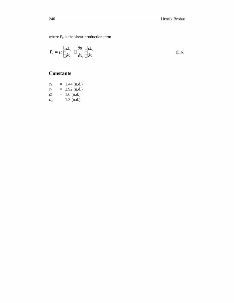
Henrik Brohus240
where Pk is the shear production term
Pu
x
u
x
u
xk ti
j
j
i
i
j
= +
µ
∂∂
∂∂
∂∂
(E.6)
Constants
c1 = 1.44 (n.d.)c2 = 1.92 (n.d.)σk = 1.0 (n.d.)σε = 1.3 (n.d.)

Appendix F t-test 241
Appendix F
t-test
In order to test the following hypothesis, regarding the flow in a displacementventilated room, a statistical test is performed.: Concentration assessed afterholding the breath is significantly lower than the concentration assessed by theimmediate impression.
Members of a Trained Sensory Panel perceived the air quality both as the“immediate impression” and “after holding the breath”. In Table F.1. thedifferences between the two assessments (in decipol) are summarised for each ofthe panel members. A paired t-test has been made assuming random sampling andblocking with pairs in persons.
If random sampling is assumed and there are n differences d, then the quantity t0is distributed as t with n -1 degrees of freedom (Box et al., 1978)
td
s
nd
0 =− δ
(F.1)
where
d = Average of the n differences (decipol)δ = True mean difference (decipol)
and the null hypothesis is δ = 0. The standard deviation, sd, is found by
( )s
dd
nnd
2
2
2
1=
−
−
∑∑ (F.2)

Henrik Brohus242
Table F.1. Summarised results of assessments by the members of a TrainedSensory Panel. A: Assessment as “immediate impression”. B: Assessment “afterholding the breath”. The results are calibrated according to Chapter 2.4.
Person B - ACase 1 Case 2 Case 3 No contamination
123456789101112
20.90-10.13-7.442.80-8.25-6.691.24-6.85-5.41-4.832.274.29
5.30-12.91-3.42-1.12-5.12-3.09-1.82-4.733.23-1.10none-4.95
-14.843.83-2.18-2.28-4.04-2.880.89-5.103.89-0.742.011.38
-0.53-2.59-3.19-1.12-2.68-0.840.570.00-0.82-0.29-0.920.00
n 12 11 12 12d -1.508 -2.703 -1.679 -1.034
d∑ -18.10 -29.73 -20.06 -12.41
d 2∑ 840.05 305.30 317.89 28.24
s nd / 2.4814 1.4300 1.4677 0.3416
t0 -0.61 -1.89 -1.14 -3.03
( )Pr t t≥ 00.28 0.044 0.15 0.0055
Sign. at level 40 % 5 % 25 % 1 %

Sammendrag på dansk 243
Sammendrag på dansk
Formål
Udgangspunktet for nærværende Ph.D.-afhandling “Personeksponering forforureningskilder i ventilerede rum” er det faktum, at mange mennesker i deindustrialiserede lande tilbringer mere end 90% af deres tid i et mere eller mindrekunstigt skabt klima, fx kontorer, fabrikker, offentlige bygninger, hjem,transportmidler, osv.
Indeklimaet er ofte påvirket af forskellige forureningskilder, der influerer påmenneskers sundhed og oplevelse af luftkvalitet, hvilket understreger behovet foren korrekt fastsættelse af eksponeringen.
Normalt antager eksponeringsmodeller, at luften og forureningen i det enkelte rumer fuldt opblandet og dermed uden koncentrationsgradienter. På den måde kaneksponeringen fastsættes alene på baggrund af en kildestyrke og en luftmængde.
I praksis vil der dog altid forekomme koncentrationsgradienter i større ellermindre grad, fx tæt på forureningskilderne eller i fortrængningsventilerede rum,hvor lagdeling af strømningen og en vertikal koncentrationsgradient netopanvendes til at forbedre ventilationseffektiviteten.
Når koncentrationsgradienter forekommer i ventilerede rum, vil tilstede-værelsenaf personer kunne påvirke det lokale koncentrationsfelt betydeligt, blandt andet pågrund af:
… at kroppens overtemperatur i forhold til omgivelserne genererer en kon-vektivopadstigende luftstrøm langs personen. Denne konvektive strømning kan medriveforurening i den nederste del af rummet og transportere den til åndingszonen.Herved kan personen blive eksponeret for koncentrationer, som afviger betydeligtfra den generelle koncentration i indåndingshøjden i andre dele af rummet.
… at personen lokalt kan virke som en forhindring for den generelle strømning.Hvis personen er udsat for en strømning bagfra, vil der dannes et kølvand foran

Henrik Brohus244
personen. Kølvandet kan medrive forureninger fra horisontale afstande på mereend en halv meter til åndingszonen.
… at personens bevægelser kan påvirke strømningsfeltet og forurenings-fordelingen betydeligt. Blandt andet vil effekten af grænselagsstrømningen aftage.
Ovenstående diskussion rejser behovet for forbedrede eksponeringsmodeller, dertager hensyn til såvel koncentrationsgradienter som den lokale indflydelse afpersoner.
Værktøjer til bestemmelse af personeksponering
Tre forskellige værktøjer til bestemmelse af personeksponering er præsenteret
1. En termisk mannequin med åndingsfunktion, hvilket er en opvarmetfuldskalamodel af en kvinde udstyret med en kunstig lunge. Forureningensimuleres med sporgas.
2. En computersimuleret person, hvilket er en numerisk model af en personanvendt i Computational Fluid Dynamics (CFD = numerisk strømnings-dynamik).Her bestemmes strømningsfeltet og forureningstransporten ved hjælp afcomputersimulering.
3. Et trænet sensorisk panel, hvilket er en gruppe personer trænet til at bedømmeluftkvaliteten i sammenligning med referencer, hvor niveauerne af oplevetluftkvalitet er kendte.
De tre værktøjer tager alle hensyn til den lokale effekt af personer, der befindersig i ventilerede rum med koncentrationsgradienter.
Værktøjerne er anvendt på de to væsentligste principper for rumventilation,nemlig fortrængningsprincippet og opblandingsprincippet. Det sker både for atafprøve værktøjerne på en række cases, men også for at undersøge hvor stor eneffekt det har på fastsættelsen af eksponeringen, at der tages hensyn til gradienterog personer ved de to nævnte ventilationsprincipper.
Mannequinen er meget anvendelig ved stationære eksponeringsmålinger, hvorforureningsspredning simuleres med sporgas. Ved hjælp af den kunstige lunge kanforureningskoncentrationen i den inhalerede luft nemt bestemmes.

Sammendrag på dansk 245
Det trænede sensoriske panel kan naturligvis benyttes til bestemmelse af denoplevede luftkvalitet, men også til bestemmelse af forureningskoncentrationen iden inhalerede luft, hvis sammenhængen mellem koncentration og oplevetluftkvalitet kendes. Det er tilfældet for referencegassen 2-propanon. For at undgåtilvænning er panelets bedømmelse dog begrænset til én inhalering.
Hvis den computersimulerede person skal anvendes, kræves et godt kendskab tilCFD, blandt andet for at bestemme randbetingelser m.v. som er afgørende for etgodt resultat af beregningerne.
De tre værktøjer er begrænset til målinger/simuleringer af gasformigeforureninger og mindre partikler (< 10 µm), hvor eksponeringen alene finder stedved respiration gennem mund eller næse.
Målingerne med den termiske mannequin stemmer godt overens med resultaterfundet i litteraturen. Der er fundet nogen afvigelse mellem person-eksponeringenbestemt ved hjælp af mannequinen og den computersimulerede person, men alleresultater er dog af samme størrelsesorden, ligesom alle væsentligestrømningsfænomener omkring en person er genfundet ved computermodellen.Simuleringerne viser, at det har stor indflydelse på eksponeringen at udstyremodellen med “ben”, især hvis forureningskilden er placeret tæt ved gulvet.
Nye størrelser
Der er defineret to nye størrelser. En ny ventilationseffektivitet:personeksponeringsindekset, εe, se ligning (1.4). Personeksponeringsindeksetudtrykker den ventilationseffektivitet, som faktisk opleves af en person i etventileret rum.
Den anden størrelse er: medrivningseffektiviteten i menneskets grænselag, ηe, seligning (3.1). ηe udtrykker evnen til at tilføre (frisk) luft fra gulvområdet tilåndingszonen. Denne størrelse er anvendt i forbindelse med fortrængnings-ventilation og i en eksponeringsmodel for fortrængningsventilation.
Begge størrelser er et resultat af, at den lokale effekt af personen er inkluderet.Målinger og simuleringer har demonstreret deres evne til at udtrykke forskellenmellem den luftkvalitet der reelt eksponeres for og middelventilations-effektiviteten i opholdszonen o.l.

Henrik Brohus246
Fortrængningsventilation
Personeksponering i rum ventileret efter fortrængningsprincippet er undersøgt vedhjælp af fuldskalamålinger i to rum og computersimuleringer af forholdene i detene.
Forureningsfordelingen ved målingerne er genereret af punktkilder. “Varme”forureningskilder anvendes til at skabe den karakteristiske to-zonekoncentrationsfordeling, hvor rummet er opdelt i en renere, nedre zone og en øvre,mere forurenet zone. Opadrettede slanger placeret over varmekilder tilførerforureningen (N2O eller 2-propanon).
En “kold” (passiv) forureningskilde er anvendt til at undersøge indflydelsen afforureningskilder placeret tæt på personer. Denne kilde består af endensitetsneutral blanding af N2O og He tilført gennem en porøs skumgummibold.
I CFD simuleringerne er der foruden de to nævnte kilder også lavet beregningermed en plan kilde i form af gulvet. Denne kilde har en konstantforureningsemission.
Det er fundet, at den lagdelte strømning og de betydelige koncentrations-gradienter i et fortrængningsventileret rum nødvendiggør en fastsættelse afeksponeringen, som ikke baseres på antagelsen om fuld opblanding.
Strømningen i menneskets grænselag kan i stor udstrækning medrive luft nedenfor åndingszonen og dermed forbedre kvaliteten af indåndingsluften, nårforureningskilderne er “varme”.
Luftkvaliteten, som personen oplever i det fortrængningsventilerede rum, ersignifikant forbedret i forhold til opblandingsventilation. Forbedringen er bådefundet ved stationære kemiske målinger og sensoriske målinger, hvor det trænedepanel bedømmer den oplevede luftkvalitet.
Bevægelser forringer luftkvaliteten på grund af forstyrrelser af mennesketstermiske grænselag, som er med til at befordre den høje luftkvalitet.
En eksponeringsmodel for fortrængningsventilerede rum er foreslået. Modellentager højde for koncentrationsgradienter og indflydelsen af menneskets termiskegrænselag. Modellen er enkel at anvende ved dimensionering i praksis. Den

Sammendrag på dansk 247
forudsætter, at den karakteristiske to-zone koncentrationsfordeling er til stede, ogat de tilstedeværende personers bevægelser er forholdsvis begrænsede.
Normalt er medrivning i grænselaget en fordel, men resultaterne viser også enmulig ulempe, når passive forureningskilder forefindes i den nedre del af rummettæt ved personen. I det tilfælde forbedrer fortrængningsprincippet ikkeluftkvaliteten.
Opblandingsventilation
Eksponering i opblandingsventilerede rum er undersøgt ved hjælp af målinger ogsimuleringer af det ensartede hastighedsfelt omkring en person, der står i envindkanal. Denne strømning antages at kunne repræsentere det lokalestrømningsfelt omkring en person i et opblandingsventileret rum. Desuden er derforetaget computersimuleringer af et opblandingsventileret rum, hvor hele feltet erindbefattet.
Her er forureningen leveret af en passiv punktkilde, og for computer-simuleringerne er også gulvet i et tilfælde simuleret som en plan forurenings-kildemed en konstant emission.
Personeksponering for forureningskilder i det ensartede hastighedsfelt afhænger afbåde kildeplacering og strømningsretningen i forhold til personen.Hastighedsniveauet er også en betydende faktor.
Hvirvler genereret i kølvandet foran en person, som vender ryggen modstrømningsretningen, har en betydelig evne til at medrive forurening. Denneforurening transporteres til åndingszonen, hvor den forårsager eksponering.Resultaterne viser, at hvirvlerne kan medrive forurening i en horisontal afstand påover en halv meter.
Personeksponering målt ved hjælp af den termiske mannequin stående ivindkanalen med en forureningskilde “i hænderne” kan overstige udsugnings-koncentrationen med en faktor 50. Den samme effekt er fundet vedcomputersimuleringerne blot med et endnu højere niveau. Dette understreger klartbehovet for en forbedret fastsættelse af eksponeringen, når forure-ningskildernebefinder sig i nærheden af personer.

Henrik Brohus248
Computersimuleringerne af et opblandingsventileret rum viser, at forurenings-koncentrationen i indåndingsluften nemt kan være dobbelt så høj somudsugningskoncentrationen, selvom forureningskilden befinder sig i en storafstand fra personen.
Målinger og simuleringer viser klart, at det ikke er nok at kende den lokaleforureningskoncentration i et “tomt” rum, den lokale effekt af personen erbetydelig og bør tages i betragtning ved fastsættelse af personeksponeringen.

References 249
References
Abbott, M.B. and Basco, D.R. (1989)Computational Fluid Dynamics: An Introduction for Engineers, ISBN 0-582-01365-8, Longman Scientific & Technical, 1989.
Air Quality Criteria for Particulate Matter (1969)National Air Pollution Control Administration Publication No. AP-49,Washington, D.C.
Arpaci, V.S. and Larsen, P.S. (1984)Convection Heat Transfer, ISBN 0-13-172346-4, Prentice-Hall, Inc.
ASHRAE (1993)Handbook of Fundamentals, Physiological Principles and Thermal Comfort(Chapter 8).
Asmussen, E. and Nielsen, M. (1989)Lærebog i menneskets fysiologi, Akademisk Forlag.
ASTM-F1291 (1991)Standard Test Method for Measuring the Thermal Insulation of ClothingUsing a Heated Manikin.
Awbi, H.B. (1991)Ventilation of Buildings, E & FN Spon, ISBN 0-419-15690-9.
Awbi, H.B. (1996)A CFD Study of the Air Quality at the Breathing Zone, Proceedings ofINDOOR AIR ´96, The 7th International Conference on Indoor Air Qualityand Climate, Vol. 2, pp. 1009 - 1014, July 21 - 26, Nagoya, Japan.
Bjørn, E. and Nielsen, P.V. (1995)Merging Thermal Plumes in the Indoor Environment, Proceedings of HealthyBuildings ´95, Fourth International Conference on Healthy Buildings, Milan,Italy, 11 - 14 September, Vol. 3, pp. 1223 - 1228.
Bjørn, E. and Nielsen, P.V. (1996)Exposure due to Interacting Air Flows Between Two Persons, Proceedings ofROOMVENT ´96, 5th International Conference on Air Distribution in Rooms,Vol. 1, pp. 107 - 114, July 17 - 19, Yokohama, Japan.
Bluyssen, P.M. and Fanger, P.O. (1991)Addition of Olfs from Different Pollution Sources, determined by a TrainedPanel, Indoor Air, Vol.1, No.4, pp.414-421.

Henrik Brohus250
Bluyssen, P.M. and Lemaire, T. (1992)The Distribution of Perceived Air Quality in an Office Space - ComputerSimulations and Sensory Evaluations, Roomvent '92 , Air Distributions inRooms, Vol.3, pp. 195 - 211, Aalborg, Denmark.
Box, G.E.P., Hunter, W.G. and Hunter, J.S. (1978)Statistics for Experimenters - An Introduction to Design, Data Analysis, andModel Building, ISBN 0-471-09315-7, John Wiley & Sons.
Brohus, H. (1992)Air Flow in a Room Ventilated after the Mixing Principle with an ObstaclePlaced in the Occupied Zone, Proceedings of Fifth Nordic Seminar onComputational Mechanics, Aalborg, Denmark, pp. 146 - 150.
Brohus, H. and Nielsen, P.V. (1994a)Contaminant Distribution Around Persons in Rooms Ventilated byDisplacement Ventilation, Proceedings of Roomvent '94, Fourth InternationalConference on Air Distribution in Rooms, Cracow, Poland, Vol.1, pp. 293 -312.
Brohus, H. and Nielsen, P.V. (1994b)Personal Exposure in a Ventilated Room with Concentration Gradients,Proceedings of Healthy Buildings '94, 3rd International Conference, 22-25August, Budapest, Hungary, Vol.2, pp.559 - 564.
Brohus, H. and Nielsen, P.V. (1995)Personal Exposure to Contaminant Sources in a Uniform Velocity Field,Proceedings of Healthy Buildings ´95, Fourth International Conference onHealthy Buildings, Milan, Italy, 11 - 14 September, Vol. 3, pp. 1555 - 1560.
Brohus, H. and Nielsen, P.V. (1996a)CFD Models of Persons Evaluated by Full-Scale Wind Channel Experiments,Proceedings of Roomvent ´96, 5th International Conference on AirDistribution in Rooms, July 17 - 19, Yokohama, Japan,Vol.2, pp.137 - 144.
Brohus, H. and Nielsen, P.V. (1996b)Personal Exposure in Displacement Ventilated Rooms, Indoor Air, Vol. 6, No.3, pp. 157 - 167.
Brohus, H., Knudsen, H.N., Nielsen, P.V., Clausen, G. and Fanger, P.O. (1996)Perceived Air Quality in a Displacement Ventilated Room, Proceedings ofIndoor Air ´96, The 7th International Conference on Indoor Air Quality andClimate, July 21 - 26, Nagoya, Japan, Vol. 1, pp. 811 - 816.
CEN prENV 1752 (1994)Ventilation for Buildings: Design Criteria for the Indoor Environment.
Christensen, R. and Stevnhoved, L. (1993)Private communication, Aalborg University.
Clark, R.P. and Edholm, O.G. (1985)

References 251
Man and his Thermal Environment, Edward Arnold (Publishers) Ltd., ISBN0-7131-4445-9.
Clark, R.P. and Cox, R.N. (1973)The Generation of Aerosols from the Human Body, In: AirborneTransmission and Airborne Infection. Ed. Hers,J.F.P. & K.C. Winkler,Oosthoek, Holland.
Clark, R.P. and Toy, N. (1975a)Natural Convection Around the Human Head, J. Physiol. No. 244, pp.283-293.
Clark, R.P. and Toy, N. (1975b)Forced Convection Around the Human Head, J. Physiol. No. 244, pp.295-302.
Davidson, L. and Nielsen, P.V. (1995)Calculation of the Two-Dimensional Airflow in Facial Regions and NasalCavity using an Unstructured Finite Volume Solver, ISSN 1395-7953 R9539,Dept. of Building Technology and Structural Engineering, Aalborg University.
Davis, J.C. (1986)Statistics and Data Analysis in Geology, John Wiley & Sons,ISBN 0-471-08079-9.
DS/INSTA 353 (1989)Beskyttelsesbeklædning, Klæder mod kulde. Termisk dukke til prøvning afvarmeisolans.
DuBois, D. and DuBois, E.F. (1916)A Formula to Estimate Approximate Surface Area, if Height and Weight areknown, Archives of Internal Medicine, 17:863-71.
Dunnett, S.J. (1994)A Numerical Study of the Factors Affecting Worker Exposure toContaminants, J. Aerosol Science, Vol.25, Suppl.1.
ECA (1991)European Concerted Action "Indoor Air Quality and its Impact on Man":“Effects of Indoor Air Pollution on Human Health”. Report No. 10,Commission of the European Communities, Luxembourg.
ECA (1992)European Concerted Action "Indoor Air Quality and its Impact on Man":“Guidelines for Ventilation Requirements in Buildings”. Report No. 11,Commission of the European Communities, Luxembourg.
Etheridge, D.W. and Sandberg, M. (1996)Building Ventilation: Theory and Measurement, ISBN 0 471 96087 X, JohnWiley & Sons Ltd.
Fanger, P.O. (1972)

Henrik Brohus252
Thermal Comfort - Analysis and Applications in Environmental Engineering,McGraw-Hill Book Company, ISBN 0-07-019915-9.
Fanger, P.O. (1988)Introduction of the olf and the decipol Units to Quantify Air PollutionPerceived by Humans Indoors and Outdoors, Energy and Buildings, 12, 1-6.
Fanger, P.O. (1995)International Trends in Ventilation Standards, Proceedings of HealthyBuildings ´95, Fourth International Conference on Healthy Buildings, Milan,Italy, 11 - 14 September, Vol. 1, pp. 257 - 263.
Fitzner,K. (1996)Displacement Ventilation and Cooled Ceilings, Results of Laboratory Testsand Practical Installations, Proceedings of Indoor Air ´96, Vol. 1, pp. 41-50,Nagoya, Japan.
Fletcher, B. and Johnson, A.E. (1988)Comparison of Personal and Area Concentration Measurements, and the useof a Manikin in Sampling, Proceedings of Ventilation '88, New York,Pergamon Press (Ed. Vincent,J.H.), pp.161-167.
Flovent (1994)FLOVENT Instruction Manual (version 1.4) and FLOVENT ReferenceManual (version 1.4), Flomerics Limited, Surrey, England.
Flynn, M.R. and Shelton, W.K. (1990)Factors Affecting the Design of Local Exhaust Ventilation for the Control ofContaminants from Hand-Held Sources, Appl. Occup. Environ. Hyg. 5(10),pp.707-714.
Flynn, M.R. and George, D.K. (1991)Aerodynamics and Exposure Variability, Appl. Occup. Environ. Hyg. 6(1),pp. 36-39, January.
Gan, G. (1994)Numerical Method for a Full Assessment of Indoor Thermal Comfort, IndoorAir, 4, pp. 154-168.
Gan, G., Awbi, H.B. and Croome, D.J. (1993)CFD Simulation of the Indoor Environment for Ventilation Design, Presentedat the ASME 1993 Winter Meeting - Paper No. 93-WA/HT-49, NewOrleans, USA.
George, D.K., Flynn, M.R. and Goodman, R. (1990)The Impact of Boundary Layer Separation on Local Exhaust Design andWorker Exposure, Appl. Occup. Environ. Hyg. 5:501-509.
Heinsohn, R.J. (1991)Industrial Ventilation: Engineering Principles, ISBN 0-471-63703-3, New York, John Wiley & Sons.
References 253
Holman, J.P. (1989)Heat Transfer, McGraw-Hill Book Co, ISBN 0-07-100487-4.
Holmberg, R.B., Eliasson, L. , Folkesson, K. and Strindehag, O. (1990)Inhalation-Zone Air Quality Provided by Displacement Ventilation, Proceedings of Roomvent '90, International Conference on Air Distribution in Ventilated Spaces, Oslo, Norway.
Homma, H. and Yakiyama, M. (1988)Examination Of Free Convection Around Occupant’s Body Caused By ItsMetabolic Heat, ASHRAE Trans. V.94, Part 1.
Hyldgaard, C.E. (1994)Humans as a Source of Heat and Air Pollution, Proceedings of Roomvent ´94,Air Distribution in Rooms, Fourth International Conference, Vol.1, pp.413-433, Cracow, Poland.
Ichihara, M., Saitou, M., Nishimura, M. and Tanabe, S. (1996)Measurements of Convective and Radiative Heat Transfer Coefficients ofStanding Human Body by using a Thermal Manikin, Proceedings of INDOORAIR ´96, The 7th International Conference on Indoor Air Quality and Climate,Vol. 2, pp. 559 - 564, July 21 - 26, Nagoya, Japan.
Iwamoto, S. (1996)A Study on Numerical Prediction Methods of Thermal Environment aroundOccupants, Proceedings of INDOOR AIR ´96, The 7th InternationalConference on Indoor Air Quality and Climate, Vol. 1, pp. 299 - 303, July 21- 26, Nagoya, Japan.
Jayatilleke, C.L.V. (1969)The Influence of Prandtl Number and Surface Roughness on the Resistance ofthe Laminar Sub-layer to Momentum and Heat Transfer, Progress in Heat andMass Transfer, Vol. 1, pp. 193-329.
Jensen, G.P. and Nielsen, P.V. (1995)Transfer of Emission Test Data from Small Scale to Full Scale, Proceedingsof Healthy Buildings ´95, Fourth International Conference on HealthyBuildings, Milan, Italy, 11 - 14 September, Vol. 1, pp. 851 - 856.
Kato, S., Murakami, S. and Zeng, J. (1996)Numerical Analysis of Contaminant Distribution around a Human Body,Proceedings of ROOMVENT ´96, 5th International Conference on AirDistribution in Rooms, Vol. 2, pp. 129 - 136, July 17 - 19, Yokohama, Japan.
Kawamura, T., Hiwada, M., Hibino, T., Mabuchi, I. and Kumada, M. (1984)Flow around a Finite Circular Cylinder on a Flat Plate, Bull. Jpn. Soc. Mech.Eng. 27(232): pp. 2142-2151.
Kerslake, D.M. (1972)The Stress of Hot Environment, Cambridge University Press, ISBN 0 521
Henrik Brohus254
08343 5.Kim, T. and Flynn, M.R. (1991a)
Airflow Pattern Around a Worker in a Uniform Freestream, Am. Ind. Hyg.Assoc. Journal, 52(7), pp. 287-296.
Kim, T. and Flynn, M.R. (1991b)Modeling a Worker's Exposure From a Hand-Held Source in a UniformFreestream, Am. Ind. Hyg. Assoc. J., 52(11), pp.458-463.
Kim, T. and Flynn, M.R. (1992)The Effect of Contaminant Source Momentum on a Worker´s Breathing ZoneConcentration in a Uniform Freestream, Am. Ind. Hyg. Assoc. J. 53(12), pp.757-766.
Knudsen, H.N. (1994)Modelling Indoor Air Quality (in Danish), Ph.D.-thesis, Laboratory ofHeating, Ventilating and Air Conditioning, Technical University of Denmark.
Knudsen, H.N., Clausen, G. and Fanger, P.O. (1993)Prediction of Perceived Air Quality in a Space Based on Small-ScaleExperiments, Proceedings of the 6th International Conference of Indoor AirQuality and Climate INDOOR AIR ´93, Helsinki, Vol.2, pp.585-590.
Knudsen, H.N., Clausen, G. and Fanger, P.O. (1994)Characterization of Sensory Emission Rates from Materials, Proceedings ofHealthy Buildings, 3rd International Conference, Vol.1, pp.463-468,Budapest, Hungary.
Krühne, H. and Fitzner, K. (1994)Air Quality in the Breathing Zone in Rooms with Displacement Flow,Proceedings of Roomvent ´94, Air Distribution in Rooms, Fourth InternationalConference, Vol.2, pp.93-101, Cracow, Poland.
Ljungqvist, B. and Reinmüller, B. (1993)Interaction Between Air Movements and the Dispersion of Contaminants:Clean Zones with Unidirectional Air Flow, Journal of Parenteral Science andTechnology, Vol.47, No.2.
Maroni, M., Seifert, B. and Lindvall, T. (1995)Indoor Air Quality (Eds.), Elsevier Science B.V., The Netherlands, ISBN 0-444-81642-9.
Martinelli, C.A., Harley, N.H., Lippmann, M. and Cohen, B.S. (1983)Monitoring Real-time Aerosol Distribution in the Breathing Zone,Am.Ind.Hyg.Assoc.J., 44, 4, pp.280-285.
Mattsson, M. and Sandberg, M. (1994)Displacement Ventilation -Influence of Physical Activity, Proceedings ofRoomvent ´94, Air Distribution in Rooms, Fourth International Conference,Vol.2, pp.77- 92, Cracow, Poland.

References 255
McCarthy, J.F., Bearg, D.W. and Spengler, J.D. (1991)Assessment of Indoor Air Quality, Indoor Air Pollution - A Health Perspective, Ch.4 pp.82-108, Ed. Samet,J.M., Spengler,J.D., ISBN 0-8018-4124-0, The Johns Hopkins University Press.
McCullough, E.A., Jones, B.W. and Huck, J. (1985)A Comprehensive Data Base for Estimating Clothing Insulation, ASHRAE Transactions, Vol.91, Part 2, pp.29-47.
Mitchell, D. (1974)Convective heat transfer from man and other animals, Heat loss from animals and man. Ed. by J.L. Monteith & L.E. Mount, Butterworths, London.
Mundt, E. (1994)Inhaled Air in Displacement Ventilation, Proceedings of Healthy Buildings,3rd International Conference, Vol.2, pp.355-360, Budapest, Hungary.
Mundt, E. (1996)The Performance of Displacement Ventilation Systems - Experimental andTheoretical Studies, ISSN 0284 - 141X, ISRN KTH/IT/M--38--SE, Bulletinno 38, Building Services Engineering, Royal Institute of Technology,Stockholm, Sweden.
Murakami, S., Kato, S. and Zeng, J. (1995)Development of a Computational Thermal Manikin - CFD Analysis ofThermal Environment around Human Body, Proceedings of Tsinghua-HVAC-´95, Beijing, Vol. 2, pp.349 - 354.
Murakami, S., Kato, S. and Zeng, J. (1996)CFD Analysis of Thermal Environment around Human Body, Proceedings ofINDOOR AIR ´96, The 7th International Conference on Indoor Air Qualityand Climate, Vol. 2, pp. 479 - 484, July 21 - 26, Nagoya, Japan.
Nickel, J. (1990)Air Quality in a Conference Room with Tobacco Smoking Ventilated withMixed or Displacement Ventilation, Proceedings of Roomvent ´90,Engineering Aero- and Thermodynamics of Ventilated Room, SecondInternational Conference, Session D2-4 (64), Oslo, Norway.
Nielsen, P.V. (1981)Contaminant Distribution in Industrial Areas with Forced Ventilation and Two-Dimensional Flow, IIR-Joint Meeting, Commission E1, Essen,Germany.
Nielsen, P.V. (1990)Specification of a Two-Dimensional Test Case, International Energy Agency,Energy Conservation in Buildings and Community Systems, Annex 20: AirFlow Pattern Within Buildings, ISSN 0902-7513, R9040, Department of
Henrik Brohus256
Building Technology and Structural Engineering, Aalborg Univesity,Denmark.
Nielsen, P.V. (1993)Displacement Ventilation - theory and design, Department of BuildingTechnology and Structural Engineering, Aalborg University, ISSN 0902-8002U9306.
Nielsen, P.V. (1996)Temperature Distribution in a Displacement Ventilated Room, Proceedings of Roomvent ´96, 5th International Conference on Air Distribution in Rooms, July 17 - 19, Yokohama, Japan,Vol.3, pp.323 - 330.
Nielsen, M. and Pedersen, L. (1952)Studies on the Heat Loss by Radiation and Convection from the Clothed Human Body, Acta Phys. Scandinav., Vol.27, pp.272-294.
Niwa, K., Murakami, S., Kato, S., Kondo, Y. and Kitamura, N. (1996)Numerical Analysis of Flow and Temperature Fields with Local Air-Conditioning by Supply Jets from the Seats in Hall, Proceedings ofROOMVENT ´96, 5th International Conference on Air Distribution in Rooms,Vol. 2, pp. 307 - 314, July 17 - 19, Yokohama, Japan.
Ott, W.R. (1985)Total human exposure, Environmental Science and Technology, Vol.19,No.10, pp.880-886.
Patankar, S.V. (1980)Numerical Heat Transfer and Fluid Flow, Hemisphere PublishingCorporation.
Patankar, S.V. and Spalding, D.B. (1970)Heat and Mass Transfer in Boundary Layers - a general calculation procedure,International Textbook Company Ltd, ISBN 0 7002 0154 8, London.
Pejtersen, J. and Mayer, E. (1993)Performance of a Panel Trained to Assess Perceived Air Quality, Proc. 6th.International Conference on Indoor Air Quality and Climate, Indoor Air ´93,Helsinki, Vol.1, pp.95-100.
Pleil, J.D. and Lindstrom, A.B. (1995)Sampling and Analysis of Exhaled Human Breath as an Exposure Assessment,Proceedings of Healthy Buildings ´95, Fourth International Conference onHealthy Buildings, Milan, Italy, 11 - 14 September, Vol. 1, pp. 507 - 511.
Rapp, G.M. (1973)Convective heat transfer and convective coefficients of nude man, cylindersand spheres at low air velocities, ASHRAE Transactions, Vol.79, part 1, pp.75-87.
Rodes, C.E., Kamens, R.M. and Wiener, R.W. (1991)
References 257
The Significance and Characteristics of the Personal Activity Cloud onExposure Assessment Measurement for Indoor Contaminants, Indoor Air, Vol.2, No. 1, pp.123-145.
Rodes, C.E., Kamens, R.M. and Wiener, R.W. (1995)Experimental Considerations for the Study of Contaminant Dispersion Nearthe Body, Am. Ind. Hyg. Assoc. J., 56:535-545.
Rodi, W. (1980)Turbulence Models and their Application in Hydraulics - A State of the ArtReview, University of Karlsruhe, Germany.
Schlichting, H. (1979)Boundary-Layer Theory, McGraw-Hill Publishing Company, ISBN 0-07-055334-3.
Sexton, K. and Ryan, P.B. (1988)Assessment of Human Exposure to Air Pollution: Methods, Measurements,and Models, In: . Watson, A.Y., Bates, R.R. and Kennedy, D. (eds) AirPollution, the Automobile, and Public Health, Washington D.C., NationalAcademy Press, ISBN 0-309-03726-3, pp.207-238.
Skistad, H. (1994)Displacement Ventilation, ISBN 0 86380 147 1, Research Studies Press Ltd.,John Wiley & Sons Inc.
Stymne, H., Sandberg, M. and Mattsson, M. (1991)Dispersion pattern of contaminants in a displacement ventilated room -implications for demand control, Proceedings of 12th AIVC Conference,Ottawa, Canada.
Surfer (1991)SURFER, Reference Manual, Version 4, Golden Software, Inc., Golden,Colorado, USA.
Säteri, J.O. (1992a)Local Ventilation Effectiveness in the Breathing Zone, InternationalSymposium on Room Air Convection and Ventilation Effectiveness, pp. 307 -312, Tokyo, Japan.
Säteri, J.O. (1992b)A Breathing Manikin For Measuring Local Thermal Ventilation Effectiveness,Proceedings of Roomvent '92, Air Distribution in Rooms, Third InternationalConference, Vol.3, pp. 167 - 179, Aalborg, Denmark.
Tanabe, S., Arens, E.A., Bauman, F.S., Zhang, H. and Madsen, T.L. (1994)Evaluating Thermal Environments by Using a Thermal Manikin with Controlled Skin Surface Temperature, ASHRAE Transactions, 3739, Vol. 100, Part 1, pp.39-48.
Tjelflaat, P.O. (1992)

Henrik Brohus258
Evaluation of Ventilation Effectiveness and Worker Exposure at the DesignStage, Proceedings of ISRACVE, pp. 154-164, Tokyo, Japan.
Tjelflaat, P.O. and Knott, R. (1996)A Simulation Model for Thermal Comfort of a Person in a Large Enclosure,Proceedings of INDOOR AIR ´96, The 7th International Conference on IndoorAir Quality and Climate, Vol. 2, pp. 1015 - 1020, July 21 - 26, Nagoya,Japan.
Turiel, I. (1985)Indoor Air Quality and Human Health, Stanford University Press, Stanford, California, USA.
Ultman, J.S. (1988)Transport and Uptake of Inhaled Gases, In: Air Pollution, the Automobile,
and Public Health. Eds. A.Y. Watson, R.R. Bates and D. Kennedy, NationalAcademy Press, Washington D.C.,ISBN 0-309-03726-3, pp.323-366.
Wargocki, P., Clausen, G. and Fanger, P.O. (1996)Field Study on Addition of Indoor Air Sensory Pollution Sources, Proceedings of Indoor Air ´96, The 7th International Conference on Indoor Air Quality and Climate, July 21 - 26, Nagoya, Japan, Vol. 4, pp. 307 - 312.
Wyon, D. and Sandberg, M. (1990)Thermal Manikin Prediction of Discomfort due to Displacement Ventilation,ASHRAE Transaction 96, 1, 3307, pp.67-75.
Åstrand, P.-O. and Rodahl, K. (1986)Textbook of Work Physiology - Physiological Bases of Exercise, McGraw-Hill, Inc., ISBN 0-07-100114-X.

Nomenclature 259
Nomenclature
Symbols
c Concentration (ppm or kg/kg or decipol)c* Dimensionless concentration (c/cR) (n.d.)c Mean concentration in the room (ppm or kg/kg)ce Personal exposure (ppm or kg/kg or decipol)cf Concentration at the floor (ppm or kg/kg)coc Mean concentration in the occupied zone (ppm or kg/kg)cout Perceived air quality of outdoor air (decipol)cp Specific heat at constant pressure (J/kg°C)cP Concentration at point P (ppm or kg/kg)cR Concentration in return opening (ppm or kg/kg)cst Average steady-state concentration in recirculation zone (ppm)d Difference (decipol)d Average of differences (decipol)f Frequency of vortex shedding (s-1)fcl Clothing area factor (n.d.)feff Effective radiation area factor (n.d.)fres Frequency of respiration (min-1)g Gravitational acceleration (m/s2)hc Convective heat transfer coefficient (W/m2°C)hfg Heat of vaporisation of water (e.g. 2.43⋅106 J/kg)hr Linear radiative heat transfer coefficient (W/m2°C)k Thermal conductivity (W/m°C)k Turbulent kinetic energy (J/kg)kp Turbulent kinetic energy at first grid node next to surface (J/kg)�me Dose rate of inhaled contaminant (kg/s)
med Dose of inhaled contaminant (kg)mp,sk Permeance coefficient of the skin ( 1.271⋅10-9 kg/(m2 s Pa) )�mr Exhaust air flow (m3/s)
�mres Pulmonary ventilation rate (kg/s)
n Air change rate (h-1)
Henrik Brohus260
n Number of differences (n.d.)p Pressure (Pa or N/m2)pa Water vapour pressure in the ambient air (Pa)ps Saturated water vapour pressure at skin surface (Pa)q Air flow rate (m3/s or m3/h or l/(s olf))qout Ventilation rate of unpolluted air (m3/s)qst Air flow out of the recirculation zone (m3/s)r Distance from exhaust opening (m)sd Standard deviation (decipol)sij Strain rate of fluctuating flow (s-1)t Temperature (°C)t* Dimensionless temperature (t - t0)/(tR - t0) (n.d.)t0 Supply air temperature (°C)ta Ambient air temperature (°C)tcl Mean temperature of outer surface of the clothed body (°C)tex Temperature of exhaled air (°C)t r Mean radiant temperature (°C)
tref Reference temperature (°C)tR Return air temperature (°C)ts Skin temperature (°C)u, v, w Mean velocity components of the x, y and z direction (m/s)u´, v´, w´ Fluctuating velocity components do. (m/s)ui Mean velocity component of the i direction (m/s)ui´ Fluctuating velocity component of the i direction (m/s)ur Velocity at distance r (m/s)uτ Friction velocity (m/s)u+, v+, w+ Dimensionless velocity (n.d.)w Weight function (n.d.)x, y, z, xi Co-ordinate directions (m)x+, y+, z+ Dimensionless distance to wall in x, y and z directions (n.d.)ye Breathing zone height (m)yoc Height of the occupied zone (m)yp Distance from wall to first grid node adjacent to surface (m)yP Vertical location of point P (m)yst Stratification height (m)
Acl Clothed area (m2)ADu DuBois surface area (m2)Aeff Effective radiation area (m2)AEx Exhaust opening (m2)

Nomenclature 261
Ar Archimedes number (n.d.), see equation (2.18)Bi Volume force in i direction (N/m3)C Rate of convective heat transfer from skin (W/m2)Cres Rate of convective heat loss from respiration (W/m2)D Characteristic length (m)D Chest width of person (m)D Diffusivity (m2/s)Deff Effective diffusivity (m2/s)Dt Turbulent diffusivity (m2/s)Ed Latent heat loss by diffusion through the skin (W/m2)Eres Rate of evaporative heat loss from respiration (W/m2)Es Latent heat loss (W/m2)Esk Rate of total evaporative heat loss from skin (W/m2)Esw Latent heat loss by sweating (W/m2)FP-N Angle factor between a person and surface N (n.d.)Geq Source strength of ventilation equipment (olf)Gk Buoyancy term (J/m3 s)Gn Pollution source strength regarding source no. n (olf)Gr Grashof number (n.d.), see equation (2.7)H Room height (m)H Height of cylinder or person (m)Ia Insulation of air layer around person (clo)Icl Intrinsic (basic) clothing insulation (clo)IT Total thermal insulation of clothing plus air layer (clo)K Rate of conductive heat transfer from skin (W/m2)L Characteristic length (m)M Rate of metabolic heat produced (W/m2)Nu Nusselt number (n.d.), see equation (2.6)PD Percentage of dissatisfied (%)Pj Jayatilleke´s sub-layer resistance function (n.d.)Pk Shear production term (J/m3 s)Pr Prandtl number (laminar) (n.d.), see equation (2.8)Pr Probability (n.d.)Qm Total heat loss from person (W/m2)Qres Total rate of heat loss through respiration (W/m2)Qsk Total rate of heat loss through skin (W/m2)Qt Sensible heat loss (W/m2)R Rate of radiative heat transfer from skin (W/m2)R Straight line distance between mouth and point source (m)Rcl Thermal resistance of clothing (m2°C/W)
Henrik Brohus262
Re Reynolds number (n.d.), see equation (2.11)S Source strength (m3/s)S Strouhal number (n.d.), see equation (4.3)Sbody Rate of storage in body (W/m2)Sc Source term in concentration equation (kg of species/kg of air⋅s)Sk Source term in k equation (J/m3 s)Sst Contaminant flow into the recirculation zone (m3/s)St Source term in energy equation (W/m3)St Stanton number (n.d.), see equation (2.54)Su Source term in momentum equation (N/m3)Sε Source term in ε equation (J/m3 s2)Sφ Source term (general form)T Absolute temperature (K)Ta Absolute temperature of the ambient air (K)TN Absolute surface temperature of surface N (K)Tr Absolute mean radiant temperature (K)
Ts Absolute skin temperature (K)U Characteristic velocity (m/s)�Vres Pulmonary ventilation (litre/min)
VT Mean expired tidal volume (litre)
W Rate of mechanical work accomplished (W/m2)Wa Humidity ratio of exhaled air (kg H2O/kg air)We Weight (kg)Wex Humidity ratio of exhaled air (kg H2O/kg air)
α Thermal diffusivity (m2/s)β Coefficient of cubic expansion / expansivity (1/K)δ Boundary layer thickness (m)δ True mean difference (decipol)δij Kronecker delta (equals 1 for i = j and equals 0 for i ≠ j)ε Average emissivity of clothing and body area (n.d.)ε Rate of dissipation of turbulent kinetic energy (J/kg s)ε Mean ventilation effectiveness (n.d.)εe Personal exposure index (n.d.)εe,n Personal exposure index regarding source no. n (n.d.)εoc Ventilation effectiveness in the occupied zone (n.d.)εP Local ventilation index (n.d.)ηe Effectiveness of entrainment in the human boundary layer (n.d.)

Nomenclature 263
λeff Effective conductivity (W/m°C)λl Laminar thermal conductivity (W/m°C)λt Turbulent conductivity (W/m°C)µeff Effective viscosity (kg/m s)µl Laminar dynamic viscosity (kg/m s)µt Turbulent viscosity (eddy viscosity) (kg/m s)ν Kinematic viscosity (m2/s)νt Turbulent kinematic viscosity (m2/s)ρ Density (kg/m3)σ Stefan-Boltzmann constant (5.669⋅10-8 W/m2K4)σ Prandtl number (n.d.)σc Turbulent Schmidt number (n.d.)σk Turbulent Prandtl number for k (n.d.)σε Turbulent Prandtl number for ε (n.d.)σt Turbulent Prandtl number (n.d.)τ Time (s)τs Start time (s)τe Stop time (s)τw Wall shear stress (Pa or N/m2)φ Dependent variable (general form)
Γφ Diffusion coefficient (general form)∆τ Time step (s)Φ Heat load (W)Φr Radiative heat loss (W)
Constants
c1 1.44 (n.d.)c2 1.92 (n.d.)cµ 0.09 (n.d.)Kres 2.58⋅10-6 kg m2/JKres 0.1348 litre m2/(W min)σc 0.9 (n.d.)σk 1.0 (n.d.)σt 0.9 (n.d.)σε 1.3 (n.d.)

Henrik Brohus264
Abbreviations
n.d. Non-dimensionalrh Relative humidityBTM Breathing Thermal ManikinCFD Computational Fluid DynamicsCSP Computer Simulated PersonTSP Trained Sensory Panel