Persistence, Performance and Prices in Foreign

Exchange Markets1

Tarun Ramadorai2

This Draft: May 2003

1I would like to thank many people at State Street Corporation and State Street Associates for

help in obtaining and interpreting data; Atindra Barua, John Campbell, George Chacko, Josh Coval,

Gene D’Avolio, Mihir Desai, Paul O’Connell, Joshua Pollet, Jeremy Stein, Tuomo Vuolteenaho

and Joshua White for numerous useful conversations, and seminar participants in the Finance and

International Lunches at Harvard, and the finance seminar at London Business School. A very

special thanks to Ken Froot for guidance and support. I alone bear responsibility for any errors

in the text.2Harvard University, Graduate School of Business. email: tramadorai@hbs.edu

Abstract

This paper addresses a deficit in the empirical literature about markets (such as foreign

exchange and bond markets) in which traders have little anonymity and where competing

intermediaries (dealers) trade on their own account. The paper provides evidence both in

cross-section, and over time, that better performing foreign exchange traders incur lower

transactions costs. This is consistent with foreign exchange dealers bidding for information

from successful traders. The result can also be explained by the existence of traders acting

as secondary providers of liquidity in these markets, or by dealers perceiving that traders

have different price elasticities of demand, and pricing accordingly. If informed or liquidity

providing traders are offered transactions costs rebates, they have little incentive to space

their orders out over time to avoid tipping off the dealer that executes these orders. Con-

sistent with this, the paper finds that successful traders have less persistent currency order

flow. The paper conjectures that persistence arises when traders are likely to be constrained

by liquidity needs, and finds evidence to support this claim.

1 Introduction

In equity markets, trades are typically conducted anonymously, with certain exceptions such

as the ‘upstairs market’ of the NYSE, with intermediaries that do not trade on their own

account. In addition, trade disclosure in equity markets is detailed and well regulated.

In the world’s largest markets by volume,1 foreign exchange and fixed income, trades are

negotiated non-anonymously over the telephone with dealers that trade on their own account

(dual-trade). Furthermore, there are limited mandated disclosure requirements in these

markets.

For anonymous markets such as equity markets, the relationship between transaction

prices and informedness is elaborated in models like Kyle [1985] and Glosten and Milgrom

[1986]. In these models, intermediaries (market makers or dealers) condition the transaction

price on the average informedness of anonymous traders. Intermediaries raise the price

against informed traders in order to avoid adverse selection risk. In equilibrium, in the Kyle

model, informed traders attempt to disguise their order flow by gradually achieving desired

positions to avoid revealing their intentions and informedness to the market maker. These

efforts are manifest in positively autocorrelated informed order flow.

In a non-anonymous setting such as the foreign exchange market, in which dealers dual-

trade, and compete with one another to acquire and consolidate information from their

clients, the logic of the Kyle model is likely to be less relevant. Dealers in such non-

anonymous settings have the ability to set different prices for different traders, contingent on

a range of trader attributes, including informedness. This is especially true in a situation of

low post-trade transparency, in which the transaction price set by the dealer is not required

to be publicly disclosed.

Several models of non-anonymous trade and dual-trading dealers in securities markets

come to the conclusion that informed order flow will be penalized, while uninformed order

flow will be offered transactions costs rebates in such settings.2 However, another possibility

is that dealers might ‘bid’ for informed traders. They could do so by rebating transactions

costs for better performing traders, thus attracting their order flow. Dealers can subse-

quently use the information contained in the resultant order flow to trade in the inter-dealer

1Daily global turnover in the foreign exchange market for the year 2000 averaged $1.1 trillion U.S. (Source:

BIS survey; Lehman Brothers).2See below for a more detailed summary of the literature on non-anonymity and dual-trading.

1

market. Consequently, informed order flow is likely to be less persistent as dealers would

welcome the opportunity to monopolize the information content of such trades. This view

is elucidated in the model of Naik, Neuberger and Vishwanathan [1999]. They predict that

a dual-trading dealer will rebate the transaction price to informed traders, earning little on

the spread on such trades, in order to exploit this information in follow-on trading.

This paper employs a detailed analysis of trading behavior in the foreign exchange market

to investigate the relationship between the performance of traders (intended to capture

their informedness), dealer price-setting, and the persistence of order flow in non-anonymous

markets. In doing so, the paper provides several results indicating that non-anonymous

markets behave in a manner that is quite distinct from the predictions of the standard

models in anonymous settings. First, the paper provides evidence in cross-section that

better performing funds receive better execution through lower transaction prices. Second,

the paper shows in time-series that controlling for past transactions costs incurred, funds

that earn high returns over 60 days get better rates on subsequent transactions. Third,

the paper establishes that better performing funds have less persistent currency order flow,

indicating that informed traders have incentives to do their foreign exchange trades in large

blocks. Fourth, the paper provides some evidence that those funds that do have more

persistent order flow suffer from worse execution. Finally, the paper provides evidence

consistent with foreign exchange flow persistence being driven by liquidity or rebalancing

needs. Taken together, these results suggest that non-anonymous markets are characterized

by trading behavior that appears opposite to the characterization provided in well-known

models of anonymous trade in equity markets.

The measure of transaction costs employed in this paper (the effective spread) is noisy.

The data are not time-stamped, hence only the day on which a transaction occurred is

known. In the paper, the effective spread on a transaction is measured as the distance

between the transaction price and the close spot foreign exchange price on the day prior to

which a fund conducted the transaction. This measure would be exact if and only if the

fund transacted at the previous day’s close (the open). To the extent that funds transacted

later than this time, the measure cannot identify exactly where in the spread the transaction

occurred.3 This admits the possibility of alternative explanations of the results.

3The choice of daily benchmark does not affect my measure of transactions costs. Mean spreads computed

using prior close, current day’s close and the average of the two have a correlation of greater than 90% stacked

across all fund-currency pairs.

2

First, these results are consistent with the existence of ‘auxiliary market-makers,’ traders

that help dealers achieve desired inventory levels by being secondary liquidity providers.

Such traders might be given transactions costs rebates for taking on positions that dealers

wish not to hold. They would also accrue returns to liquidity provision that show up as

good performance. However, this hypothesis requires that the return to liquidity provision

occurs over longer horizons than a few days, as the measure of performance employed in

this paper does not incorporate returns earned by traders on the three days surrounding a

transaction.

Second, these results could arise if dealers perceive differing price elasticities of demand

for foreign exchange, and exploit this when pricing. Assume that there are two distinct

trader types in the data. The first type is those funds that care about currency trading,

and earn high returns on currency trades. The second is composed of funds that only

purchase currencies to transact in underlying international securities, that do not care about

their performance in currencies. If dealers price discriminate, they would give the first type

of fund (high return earners) good deals on currency transactions, while the second type

will have poor measured performance (as they are not concerned with the currency portion

of their investments), and receive worse execution from dealers. This second category of

funds will also have persistent currency flow if their equity flow is persistent, generating the

observed relationship between persistence and performance. This hypothesis is certainly

plausible. However, in time series regressions, it appears that there is the possibility of

acquiring rebates conditional on good past performance. This indicates that any fund,

irrespective of the category in which it is placed, is allowed to change its performance and

hence earn better execution. If there is a ‘category effect’ it is likely just one part of the

story.

The evidence in this paper is related to the theoretical predictions and empirical evidence

on the market microstructure of asset markets with and without anonymous counterparties.

Admati and Pfleiderer [1991] predict that trades preceded by announcements that they are

purely liquidity motivated will experience lower transactions costs. Roell [1990], Forster

and George [1992] and Pagano and Roell [1996] model the effects of changing the degree of

anonymity in securities markets, and predict that liquidity traders will receive better exe-

cution when anonymity is low. Seppi [1990] finds that equilibria exist in which liquidity

3

traders will optimally trade large blocks4 in a non-anonymous ‘upstairs’ market, incurring

lower transactions costs, while informed traders will trade anonymously. This reasoning is

confirmed by Madhavan and Cheng [1997] in an empirical analysis of the upstairs market

of the NYSE. Theissen [2000] finds that liquidity traders receive better execution in the

non-anonymous Frankfurt Stock Exchange. Fishman and Longstaff [1992] show that in

commodity future markets with dual trading brokers, informed traders have lower profitabil-

ity than they would in the absence of dual trading. The empirical evidence presented in

these papers appears opposite to the findings in this paper.

The two models closest in spirit to the empirical work presented here are those of Lyons

[1996] and Naik et. al. [1999]. Both consider markets that closely mirror the foreign

exchange market structure, with non-anonymity, dual trading, low post-trade transparency

and risk-averse dealers. While Lyons’ focus is on optimal transparency of inter-dealer

trades, Naik et. al. focus on customer-dealer trade, and predict that dealers will rebate

transactions costs for trades that contain information. They also solve for the endogenous

trading strategy of an investor in their model, and find that optimal order size is positively

related to the information content of the trade, and inversely related to the liquidity shock

component of the trade. The results in this paper indicate that this model is an accurate

characterization of the foreign exchange market. However, the Naik et. al. model is

not dynamic, and does not model heterogeneity in the types of customers in the foreign

exchange market. The ‘category effect’ explanation of the results in this paper speaks

to the importance of considering cross-sectional differences in the objectives of customers

trading foreign currencies. These differences might also feed into the dynamics of their

trading strategies.

The evidence in this paper also speaks to the growing literature on international port-

folio investment flows. Authors such as Froot, O’Connell and Seasholes [2001], Seasholes

[2000] and Froot and Ramadorai [2001, 2002a] present evidence that the aggregated invest-

ment flows of institutional investors positively anticipate equity and currency returns in local

markets. This observed anticipation could be generated by superior information on the part

of these institutions, or simply by price pressure. If information lies behind the observed an-

ticipation, standard microstructure models would suggest that the response of intermediaries

4Empirical studies investigating relationships between trade size and price include Holthausen, Leftwich

and Mayers [1987], Keim and Madhavan [1996], Chan and Lakonishok [1993, 1995].

4

in local markets would be to raise prices to avoid adverse selection risk from the trades of

large foreign institutions. The results in this paper suggest that in non-anonymous currency

markets, intermediaries welcome such informed trading rather than penalize it. The paper

also demonstrates that studying the cross-section of foreign institutional traders yields rich

insights about trading behavior that are not apparent from aggregated flows.

Related empirical analyses of the foreign exchange market have not tested the predictions

of these theories directly, but instead have tended to focus on the effects of volatility and inter-

dealer competition on spreads.5 This paper addresses this deficit, employing detailed data of

foreign exchange trading by large institutional investors to do so. The funds considered here

trade a range of securities, including international equities, debt, derivatives and currencies.

Some funds use currencies to simply fund purchases of other assets, while others actively

hedge currency risk, and make speculative trades on international currency movements. The

level of detail about the cross-section of funds is quite high, enabling the measurement of

the effects of fund-specific attributes on the prices funds receive from dealers, which in turn

influences their trading behavior in several ways.

The second section discusses the nature of the data, and provides descriptive statistics.

The third section describes the empirical methodology, and the fourth section provides results

from the specifications. The fifth describes the methodology that attempts to explain

some part of the persistence of order flow as arising from liquidity motivated considerations.

Section six concludes.

2 Data

2.1 Foreign Exchange Transactions Data

The cross-border foreign exchange transactions data come from State Street Corporation

(SSC). State Street is the largest U.S. master trust bank and one of the world’s largest global

custodians. It has approximately $7 trillion of assets under custody. State Street records all

transactions in these assets, including cash, underlying securities, and derivatives. SSC sees

approximately 3-6% of total global flow in currencies as a result of its custodial business.

There are a total of 13,230 funds represented in the data, trading over 100 currencies.

Only currencies classified by the IMF as having some variant of a free float are used. This

5See Huang and Masulis [1999] and Bollerslev and Melvin [1994] for a good summary of this literature.

5

leaves 19 countries: Australia, Canada, Euroland, Japan, New Zealand, Norway, Sweden,

Switzerland, U.K., Mexico, Indonesia, Korea, Philippines, Singapore, Taiwan, Thailand,

Poland, India and South Africa. Pre-euro, Euroland is an aggregate, that represents trades

in all of the 11 Euroland countries. These trades are paired with the deutsche mark prior to

the introduction of the euro. The final sample consists of 1,275 buy-side institutional funds,

that trade at least seven of the currencies in the set, of which at least one is an emerging

market. Each fund has an active period of at least 120 days, and trades at least 50% of those

days. There are a total of 3,642,690 transactions from these funds, across all 19 currencies.

Each transaction is a cross-currency transaction, meaning that each buy is matched with a

countervailing sell. Since the preponderance of transactions (above 95%) in the data set are

conducted against the U.S. dollar, there is very little double-counting in the data.

The sample begins January 1, 1994, and continues through February 9, 2001, covering

1,855 days for the 19 countries. For a fuller description of the data and methodology used to

construct the data, see Froot and Ramadorai [2002a]. For the current study, any transaction

which has a present value of less than U.S. $1,000 for any currency is excluded to clean out

transactions that were effected for the purposes of corporate actions. This filter eliminates

less than 0.01% of the total volume for any currency, and does preserve transactions such as

income repatriation, which are likely to be in the $1,000 - $100,000 range.

The fund is the primary unit of analysis in the data. Funds are either stand-alone,

or belong to a family of funds. This would mean, for example, that a fund family X is

represented in the data by funds X1, .., XN , which may or may not follow similar strategies.

Classification at the fund level is sharp but fund family classification is not, hence the

fund is the primary unit of analysis. To the extent that families adopt similar currency

strategies, the cross-sectional variation in the data will be damped - however, in the data,

there is significant cross-sectional variation at the level of the fund. Funds trade a range of

instruments. The funds in the data are a mix of funds trading currencies, most of which are

hedging transactions in assets other than currencies, such as international equity or debt.

However, the classification ‘informed’ does apply in this case, as seen in Froot and Ramadorai

[2002a]: aggregated flows from these funds have a statistically significant ability to anticipate

movements in excess currency returns over 40 days.

6

2.2 Interest Rate and Exchange Rate Data

Interest rates for the countries over the estimation period are obtained using daily interbank

rates for the one month horizon, when available, from Datastream. If interbank rates are

unavailable for the country for the specified horizon, an available corporate rate is used,

for example, the corporate deposit rate is used as a proxy for Colombian interest rates.

If corporate rates are unavailable, the treasury bill rate over the specified horizon for the

country is used. As a final measure, if there is only one interest rate available for a specific

country, the yield curve is assumed flat in the country at the available rate.

Exchange rate daily series for each of the countries come from WM/Reuters6 via Datas-

tream. These rates, along with the interest rates, are used to construct excess currency

returns for the currencies studied in the paper.

2.3 Measuring Persistence, Performance and Prices

2.3.1 Measuring Persistence

The persistence or autocorrelation of foreign exchange order flow is likely to arise from

several sources. Persistence could arise from the conditional probability of a fund trading

a currency because it traded the same currency on days past. Alternatively, a fund might

trade today because other funds traded the same currency on prior days. Order flow might

also arise because a fund traded other currencies on prior days, because other funds traded

other currencies on prior days, or simply because of movements in excess currency returns

on prior days. This is by no means an exhaustive list, but it does capture features of herd

behavior and trend following that a priori might be expected to have first order effects on

order flow.

In the standard Kyle model, the persistence of a trader’s order flow is an index of the

informedness of the trader. The more informed the trader, the more careful the trader is to

disguise his/her information, by eking out order flow in a single security in the direction he

or she prefers, in order to reduce the price impact of the overall trade. In order to clean out

6The WMCompany publishes these rates, which are now universally used in currency analysis. According

to WM, closing spot rates are based on the rates at 16.00 U.K. time each trading day and then published at

around 16.15. The calculated rate is based on actual traded rates on the Reuters Dealing 2000-2 network,

along with other quoted rates contributed to Reuters by leading market participants.

7

all the other possible sources of persistence, so as to capture this feature of trading behavior,

a regression similar to that in Froot and Tjornhom [2002] and Froot and Ramadorai [2002b]

is estimated (see Appendix 2 for a more detailed description of this procedure), namely,

fi,k,t = c+ aoo(L)fi,k,t−1 + aco(L)Xj 6=i

fj,k,t−1 (1)

+aoc(L)Xl 6=k

fi,l,t−1 + acc(L)Xl 6=k

Xj 6=i

fj,l,t−1 + εi,k,t

Here, fi,k,t represents the flows of a fund i into a country k at time t.7 In the specifications

below, this regression is run for each fund. A ‘persistence index’ is then computed, in which

each fund’s persistence rank is determined by the average across the lag coefficients aoo(L).8

Henceforth, the persistence index, with parameters specified, will be referred to as ρ$i when

computed using U.S. dollar flows, and ρDi using digital signals of underlying flows, where 1

represents a net purchase on a day, 0 no purchase or sale, and -1 represents a net sale on the

day. The specification is run at both the daily and weekly frequencies. The coefficient aoo(L)

here identifies own-fund, own-country persistence, after cleaning out the other cross-effects

outlined above.9

2.3.2 Measuring Performance

Fund ex-post returns are computed to rank funds in terms of their performance.10 Holdings

of the funds are not available, hence returns are computed assuming that all funds start at a

zero balance, using their aggregated net flows over the life of each fund in the sample. This

is equivalent to measuring the performance of these funds over the sample period. A Sharpe

ratio measure is computed, which divides the mean return (either dollar weighted or percent

(equal weighted)) by the standard deviation of fund returns over time. As a check, the total

dollar and equal weighted return over the fund’s lifetime and the mean dollar and equal

weighted return over fund lifetime were used as performance measures. These measures

appear to correlate highly with one another, and with the measured Sharpe ratios. In what

7Henceforth, subscripts i, k, t will denote fund, country, time respectively, wherever used.8Using the largest root of the autoregressive process yields very similar results.9Incorporating excess currency returns into equation 1 does not materially alter the results.10See Appendix 3 for a detailed description of the methodology employed to compute fund returns.

8

follows, the Sharpe ratios are used, as the results are quite similar, and the Sharpe ratio

seems most theoretically sound.

Since currency excess returns are used to compute these Sharpe ratios, the returns are

already expressed over the U.S. return benchmark. rewi,k,t represents the percent return on

the balance of a fund i in a currency k at time t, while rvwi,k,t is the return expressed in dollar

terms.

SRvwi,k =

µt(rvwi,k,t)

σt(rvwi,k,t), SRew

i,k =µt(r

ewi,k,t)

σt(rewi,k,t)(2)

2.3.3 Measuring Prices - Effective Spreads

The standard method for measuring the transaction cost of trades in equity markets is the

effective spread of a trade. This concept has been used by authors such as Roll [1984], Stoll

[1989] and Huang and Stoll [1997]. It is a measure of the distance between the price at

which the trade is conducted, and the pre-existing quote midpoint in the market prevailing

at the time of the trade. Since there are no time stamps on the transactions in the data,

the effective spread on a transaction is measured relative to the close price on the day

before the transaction was conducted. This makes the spread measure noisy. However,

experimenting with different benchmarks such as current day’s close price does not affect

the results.11 Appendix 4 contains a more detailed description of the method for computing

effective spreads in the data.

The signed half effective transaction dollar amount weighted spread is denoted by zvwi,k,t

on a transaction conducted at time t, by a fund i in a currency k. The signed half effective

equal-weighted percentage spread is denoted zewi,k,t, notation as above. The mean signed half-

effective spread across all transactions conducted by a fund in each of the currency groups is

used to measure the average transaction cost for the fund. Henceforth, zvwi,k (zewi,k ) is used to

signify the mean dollar (percent) spread across all transactions conducted by a fund. Note

that spreads are signed, i.e., a positive spread represents transacting at a price worse than the

prior day’s close spot foreign exchange price, while a negative spread represents transacting

11Under the null hypothesis that a fund is not informed, any intraday return should not be in any way

systematically correlated with future returns on the transaction conducted. However, for an informed fund,

one might expect that knowledge of the future movement of a currency would be correlated with an early

trade. Hence, I measure spreads relative to the prior spot close.

9

at a better price than prior day’s close.

2.4 Descriptive Statistics

Table 1 describes the cross-section of funds in each currency. First, the cross-sectional

distributions of total absolute trades by fund and number of trades per fund are both right-

skewed, since the mean is larger than the median. This indicates that most funds have much

smaller total transact than the cross-sectional mean would indicate, but that the few funds

that are larger than the cross-sectional mean trade size have transacted very large amounts.

Second, the number of funds that transact in each currency is highest in the major currencies,

and there is a large attenuation of both the mean and the standard deviation of the number of

transactions per fund in the other currencies. In addition, the mean total absolute transact

per fund in the smaller currencies is significantly lower than that in the larger, more liquid

currencies.

Tables 2 and 3 present descriptive statistics for the persistence, performance and price

measures. Table 2 presents descriptive statistics on persistence measured using digital flows,

Sharpe ratios measured using percentage returns, and spreads in basis points, while Table

3 presents U.S. dollar flow persistence, Sharpe ratios calculated using dollar returns, and

dollar spreads (transaction amount weighted spreads).

The first point of interest is that foreign exchange order flow appears quite persistent,

though far less persistent than equity flows.12 Second, there is high dispersion in the

persistence of the foreign exchange flows across funds. Since the funds in the data are a

mix of those trading foreign exchange for the purpose of trading in other assets, and those

trading foreign exchange as an asset in its own right, this is not surprising. Third, the

digital flow persistence is higher than the dollar flow persistence reported in Table 3.13

The Sharpe ratios, on average, are very small, i.e., on average, the funds are not earning

high returns on trading currencies. However, the dispersion in performance is quite high.

The low median measured return is being generated by the preponderance of funds trading

assets other than currencies. These funds use currencies to fund these purchases of other

assets, and to hedge out exposures to currency risk. The higher performing funds are likely to

12See Froot and Tjornhom [2002] for a detailed study of equity flow persistence.13As the size of the transactions varies a great deal, simple directional indicators like the digital indicator

will give a clearer picture of the general trend of buying and selling, and the autocorrelation thereof.

10

be trading currencies for return generation, in addition to their hedging needs. Reporting

from a separate calculation, the total profit has a median of approximately -$600,000 for

the funds in the data set for all currencies, over an average trading period for all funds

of 948 trading days (approximately four years). The standard deviation of dollar profits

for all currencies is very high, on the order of U.S. $60 million. These profits seem to

be about evenly distributed between the major countries and other countries, though from

inspecting the median dollar Sharpe ratios, it seems as though the funds are doing better

in the other/emerging market countries. It is notoriously difficult to measure long-run

performance accurately. However, the cross-sectional variation in the performance measure

employed in this paper is used as a good indicator of the true cross-sectional variation.

Finally, the median spreads that funds get for all three currency groups are on the order

of 4 to 7 basis points (twice the quantity reported in Table 2, since the reported amount is

the signed half spread), which is higher than the reported spreads in the foreign exchange

market, but of a similar order of magnitude.14 The standard deviation of fund mean spreads

in the cross-section is on the order of 40 to 60 basis points, signifying that there is a good

deal of variation across funds. The high standard deviation in the measure is also due to

the noise contributed from the lack of time stamps, forcing the reliance on spot close rates

rather than intraday quotes as the spread benchmark. Furthermore, the spreads are on

average negative in the cross-section, across all measures and currency groups, indicating

that the funds appear to be transacting at rates better than the previous day’s close. In

Table 3, it is clear that the dollar spreads are quite small compared to similar numbers in

equity markets, considering the large size of the notional amounts reported in Table 1 - this

confirms the commonly accepted notion that foreign exchange markets are extremely liquid

compared to almost any other type of asset market.

3 Cross-Section and Time-Series Specifications

3.1 Cross-Sectional Specifications

First, correlations between the measures employed are estimated. Next, a cross-sectional

regression specification is employed to investigate the determinants of spreads, and to control

14Cheung, Chinn and Marsh [2000] report that DM/$, £/$, U/$ and CHF/$ all have mean spreads ofbetween 3 and 4.5 basis points.

11

for other possible determinants of variation in spreads.

Separate regressions are estimated for the percentage spreads and transaction dollar

amount weighted spreads. Transactions costs discounts are likely to be given on the large

transactions, since trade informativeness will generate lumpier trading behavior in equilib-

rium if there are transactions costs rebates for informed orders. This will make it the case

that the dollar spread regressions, though likelier to generate statistical significance, will

contain less information, since the results are likely to be driven by the largest transactions.

However, these regressions will give an idea of the dollar magnitudes of transaction cost

rebates.

Separate regressions are run for each of the currency groups: all, major and other curren-

cies, to test variation in the results across currencies. A priori, the effect should be expected

strongest for the other/emerging group of currencies, as the largest, most liquid markets are

likely more efficient, and less characterized by the existence of private information.

The baseline cross-sectional specifications are:

zvwi,k = α + βz,ρρ$i,k + βz,SRSR

vwi,k + βz,ψψi,k + βz,φφi,k + εi,k (3)

and

zewi,k = α+ βz,ρρDi,k + βz,SRSR

ewi,k + βz,ψ log(ψi,k) + βz,φ log(φi,k) + εi,k (4)

In these regressions, for each currency group, the variables are constructed for each fund

within groups of currencies.

Next, greater flexibility is allowed by estimating the equations in a panel setting, stacking

the dependent variables, the spreads, for each fund and currency. Estimating in a panel

lends greater power to the specifications, and also allows for separate country fixed effects,

to capture variation in the mean across currencies. The panel specification is:

zi,k = αi + βz,ρρi + βz,SRSRi + βz,ψψi + βz,φφi + εi,k (5)

In these panel specifications, all of the regressors are estimated over the transactions in all

currencies, as a check, since these attributes are more likely fund than currency specific.

These specifications regress mean effective spread across all transactions by each fund

on a number of fund characteristics. The first is the fund’s computed ex-post Sharpe ratio

SR. Here, ew and vw denote equal weighted (percentage) and value weighted (dollar)

12

return respectively. Clearly, incorporation of the intraday return into the measured Sharpe

ratio will generate bias in the specifications towards finding a result. In order to avoid

any mechanical contamination, returns earned on dates t − 1, t, t + 1 are removed fromcomputation of the Sharpe ratios, for any date t that a fund traded. Removal of these

returns will also help to attenuate returns that funds might earn from acting as secondary

liquidity providers, since liquidity generated returns might be expected to manifest over very

short horizons.

The second regressor is the persistence of the fund’s order flow ρ. Here $ and D denote

persistence measured using dollar flows, and digital signals respectively.

Two additional regressors are employed, to soak up variation in spreads that may be

generated by other sources. The first additional variable is a proxy for fund size ψi,k, which

is computed as ψi,k =P

j |fi,k,j| where i, k index funds and currencies respectively, and j

runs over all the days each fund is alive. This rough measure of fund size is measured as

the sum total of the absolute dollar value of a fund’s trades in each currency group.

The second regressor employed is a measure of fund daily transaction frequency, φi,k,

computed as φi,k =1Ei

PEil=1 n(τ i,k,l) where n(.) is the number of transactions conducted each

day l that a fund is active until its end date in the set Ei. φi,k is the time series mean

number of transactions per fund per currency. This measure is used as a rough estimate of

intraday persistence.

A separate cross-sectional regression investigates the relationship between performance

and persistence:

ρi,k = α+ βρ,SRSRvw,ewi,k + εi,k (6)

3.2 Interpreting the Coefficients

In these specifications, evidence of H11 : βz,SR > 0 would suggest that adverse selection risk

from informed order flow drives dealer pricing behavior. On the other hand, evidence of

H21 : βz,SR < 0 is more plausibly explained by a model such as that of Naik et. al. [1999]

in which dealers ‘pay’ for informed order flow in order to use this information in follow-

own trading in the inter-dealer market. Finding in favor of H21 is also consistent with two

alternative explanations.

The first explanation has dealers calling funds in order to unload positions that they

are not willing to keep in inventory, positions that generate a liquidity driven return over a

13

longer horizon than the few days surrounding the trade. This generates a transactions cost

rebate for liquidity provision, and the liquidity generated return, explaining the observed

negative correlation between spreads and performance.

The second explanation (henceforth termed the ‘category effect’) has dealers exploiting

different elasticities of demand in the foreign exchange market, and setting transactions

costs accordingly. Under this explanation, there are two categories of funds represented in

the data. The first category of funds pays careful attention to currency returns, and also

cares about transactions costs on currency trades. The second category of funds performs

worse on currency returns. These could be funds that take currency exposures solely for the

purposes of purchasing other assets, and have low price elasticity of demand for currencies.

Dealers that perceive these different price elasticities of demand for currency transactions

between the two categories set different transactions prices for these two different categories

of funds. This would generate the observed negative correlation between performance and

spreads.

The second hypothesis regards the role of persistence. Here, the hypothesis is H31 :

βz,ρ > 0.15 If informed traders have the incentive to diffuse and split up their trades using

uninformed intermediaries, and adverse selection risk is pervasive, one might expect worse

prices to be given to more persistent order flow, through the adverse selection channel.

However, there is another channel through which persistence in order flow would result in

higher effective spreads to traders. Evidence of H21 (which runs contrary to adverse selection

driven dealer pricing) in conjunction with H31 points to the following story. If dealers wish

to attract informed traders, informed traders will trade large blocks, rather than piecing out

their order flow. This is because follow-own trading by an informed trader does not give the

dealer as much freedom to exploit information contained in informed orders. In addition,

the dealer ‘bidding’ for order flow would prefer to attract all the order flow rather than risk

having the informed trader piece it out among multiple dealers, thus diluting the information

exploitable.

Furthermore, uninformed strategic liquidity traders will not wish to incur large trans-

actions costs generated by larger trades.16 An uninformative large trade adds more to a

15The measure φ, the mean number of transactions per day, is a rough measure of intraday persistence.

Hence, a positive coefficient βz,φ leads to a similar interpretation as βz,ρ > 0.16In the Naik et. al. [1999] model, holding information content constant, price rebates are inversely

correlated with trade size.

14

dealer’s inventory, which makes it potentially harder for the dealer to respond to the in-

formation contained in informed trades. This is reflected in a worse spread given to large

liquidity trades than to smaller liquidity trades. In equilibrium, this should result in more

persistent order flow by strategic liquidity traders who prefer to piece out their liquidity de-

mand. Their average transactions cost would still be higher than those of informed traders,

who get paid for their order flow.

Evidence in support of H21 ∩ H3

1 is consistent with the ‘category effect’ story as well.

Suppose that funds are placed in different categories by dealers depending on the extent to

which they care about the currency portion of their portfolios. If dealers perceive price

elasticity of demand to be different across categories, they might charge higher spreads to

worse performing traders, traders that do not care about currencies to the extent that they

care about returns on their trades in other assets. According to this explanation, currency

funds that receive poor execution will also have highly persistent order flow, as evidenced

by H31 . This is driven by the linkage between the persistent trades of such funds in illiquid

equities, and the currency purchases used to fund their equity purchases.

Turning to the interpretation of equation 6, evidence in favor of H41 : βρ,SR > 0 would

suggest that adverse selection is driving dealer price-setting. This is in line with the Kyle

model, in which traders with the most information would be more likely to want to disguise

their order flow from the dealer. This would result in their spacing out their trades, and

rationing them over time in order to avoid price impact.

On the other hand, evidence of H51 : βρ,SR < 0 would suggest that the Naik et. al.

model of dealer payment for order flow is a more apt characterization of the FX market. It

would also suggest that persistence is a characteristic of liquidity traders as stipulated above.

Such a finding is also consistent with the ‘category effect’ explanation. If funds that perform

worse in currencies are primarily investing in equities, the illiquidity of equity markets could

generate high equity flow persistence. This persistence then gets translated through to their

currency purchases. Purchasing foreign exchange in large volumes may be better, if there

is information associated with both foreign exchange and equities and the logic of ‘bidding

for information’ holds, or if there are size discounts offered in foreign exchange. However,

holding large quantities of foreign exchange may generate a risk imbalance for managers pri-

marily interested in illiquid equities. It may, therefore, be constrained optimal for managers

that do not care about their performance in currencies, to let their equity trading behavior

15

dictate their foreign exchange purchases, generating persistent foreign exchange order flow.17

Finally, the fund size measure is expected to have a negative coefficient, if dealers rebate

transactions costs for large funds that are expected to transact high volumes. The dealer

can make money off the volume from such funds, amortizing the lower transactions costs

over larger dollar trades.

3.3 Time-Series Methodology

In time series, an additional insight into the relationship between performance of funds and

the execution received from the dealer can be obtained by running a Granger causality test

between returns and spreads. This methodology can be used to test whether transactions

prices are sensitive to changes in returns earned by a trader. The specification employed here

does not distinguish between luck and performance - perception of good trading generated

by higher accrued returns on a trader’s position over the prior few months is treated just

the same as true skill.

Returns for a fund i in a currency k at time t are denoted as ri,k,t. The spread is, as

before, denoted by zi,k,t. The specification estimated is:

zi,k,t = αi + Γz(L)zi,k,t−1 + Γr(L)ri,k,t−1 + εi,k,t (7)

Granger causality then tests the hypothesis Γr(L) = 0.

The null hypothesis H60 is therefore that r does not Granger cause z in the above re-

gression. Rejection of the null withP

L Γr(L) < 0 is evidence in favour of more favorable

execution in response to higher returns earned. Clearly, the more natural test would be to

use cumulated returns up until time t − 1 instead of returns. However, since cumulated

returns would be expected to be I(1), putting them into an autoregression would throw off

inferences. In order to capture lower frequency dynamics, therefore, lags of up to three

months (60 trading days) are incorporated in the regression. To help interpretation, conti-

nuity restrictions are imposed on the coefficients by aggregating all daily lags 1-60, forcing

the coefficients within the aggregation to be identical. The interpretation of individual co-

efficients on daily lags for the purposes of this study is not quite as important as the overall

picture garnered from the effect of prior returns on the spread.

17Thanks to Ken Froot for useful conversations about this.

16

Rejection of the null will also provide evidence indicating that the ‘category effect’ story

cannot be a complete explanation of the results. According to this story, funds that purchase

currencies solely to transact in underlying international securities do not care about their

performance in currencies, and receive worse execution from dealers that perceive that they

have relatively inelastic demand. Funds that care about currencies and perform well in them

will receive better execution. Rejection of the null here indicates that controlling for past

transactions costs incurred, funds that earn high returns over 60 days, will receive better

execution on subsequent transactions. This would suggest that even within categories of

traders, there is the possibility of acquiring rebates conditional on recent good performance.

There are several estimation issues that arise in this context. First, in the cross-sectional

context, returns accrued on days t− 1, t, t+ 1 were removed when a trade occurred on datet, to avoid generating any mechanical association between the measure of performance and

that of transaction costs. This is no longer necessary in the context of the autoregression,

since lagged spreads are also in the specification, creating a natural control. Note also that

since spreads are measured relative to prior day’s close, that any positive autocorrelation in

currency returns earned by funds that leads to future successful intraday trading would bias

against finding a measured negative coefficient Γr(L). Second, only days on which a fund

trades are used in the autoregression. Thus, the autoregression can be considered a trading-

day by trading-day specification. Finally, standard errors corrected using the Newey-West

procedure are reported, using 60 lags of the residuals to clean out all possible autocorrelation

induced from the overlapping returns employed.

4 Results

4.1 Results from Cross-Sectional Analysis

Table 4 presents correlation coefficients between the measures of persistence, performance

and prices. The first feature worth noting is that the measures of persistence are very highly

correlated with one another18 Second, measures of returns appear to correlate quite well with

one another. Funds that have high dollar Sharpe ratios usually have high equal weighted

18Persistence measured using weekly data correlates very highly with persistence measured using daily

data. Further, the rankings generated by dollar persistence and those from digital persistence correlate very

highly with one another.

17

Sharpe ratios. These correlations are in the 59% to 75% range for the two measures, for all

three of the country groupings.

Second, there is a measured negative correlation between the measures of persistence and

those of performance. For dollar Sharpe ratios, this correlation varies between -7% and -

14%, with both measures of persistence (using only the statistically significant correlations).

For equal weighted returns, the result is approximately similar - there is a statistically

significant measured negative correlation between equal weighted performance measures and

the measures of persistence of between -5% and -8%. This result holds true across all the

groups of currencies, with the single (not statistically significant) exception of the major

countries, in which the equal weighted Sharpe ratios are slightly positively correlated with

the dollar persistence measure. At first pass, therefore, it appears that there is a negative

relationship between access to information on the part of traders and the persistence of their

order flow.

Third, persistence and prices are positively related, primarily for the non-major countries

in the sample - the dealer appears to charge higher transaction prices for those traders who

have more persistent order flow. This in combination with the negative relationship between

performance and persistence, and the results below, favors the hypothesis that persistence

in foreign exchange order flow is driven by traders with portfolio rebalancing or liquidity

motivated trading needs.

Fourth, there appears to be a negative relationship between performance and prices - the

dealer gives better transaction prices to traders who earn higher returns in currency trading.

This indicates that the dealer learns from the order flow of such traders, and wishes to give

them better transaction prices in order to attract their valuable order flow. As stated earlier,

this is also consistent with an alternative hypothesis in which the dealer calls customers that

are ‘auxiliary market makers’ in order to off-load an undesirable position, that generates a

liquidity generated return over a longer horizon. However, this hypothesis requires that the

liquidity generated return manifests over horizons longer than the three days surrounding the

currency transaction, since the measured Sharpe ratio does not incorporate returns earned

by funds on these days.19 The finding is also consistent with the ‘category effect’ explanation

outlined earlier.

Inspecting Table 5, which estimates equation 4, for all countries, there is a negative

19In addition, this explanation is not consistent with anecdotal reasoning in the foreign exchange market.

18

relationship between performance and prices. This points to a situation in which market

makers are prepared to give better execution to those funds they perceive as being better

informed, in order to learn from their order flow about future prospects in the market. In

terms of the equal weighted (geometric) Sharpe ratio, the magnitudes reveal that a 100 basis

point upward move in the geometric Sharpe ratio will result in an approximately 0.1 basis

point lower transaction cost on average over all its transactions. This is significant at the

7% level for all countries, though not statistically significant for either of the other currency

groups in isolation. In Table 6, which dollar weights the spreads by their transaction

amounts, estimating equation 3, the magnitudes indicate that a fund that has a 100 basis

point upward move in its dollar (arithmetic) Sharpe ratio, will get an approximately U.S.

$32 lower transaction cost from the dealer on average over all its transactions. This is

highly statistically significant for all countries. The same approximate magnitude is true

for the non-major countries in the sample, though the statistical significance is somewhat

lower. The result in the entire cross-section of countries is predominantly being driven by

the non-major countries in the sample.

This finding leads to the expectation that better performing foreign exchange traders

have no need to disguise their order flow from the dealer. In Table 9, this is made clear.

Funds that are better performers tend to have less persistent order flow. A fund that has a

Sharpe ratio that is higher by 10% tends to have persistence that is lower by about 1.5% for

value weighted flows. The association is statistically significant and negatively signed for all

the measures considered. This, together with the results above, points in the direction of a

liquidity motivated reason for persistence, in which information is not about future return

prospects, but rather about own future demands. This is also consistent with the ‘category

effect’ explanation.

Returning to Tables 5 and 6, note that there is a weak statistically positive association

between prices given by the dealer and the persistence characteristics of the order flow of

funds in the cross-section. The coefficient in Table 6 indicates that a 5% move in the

persistence index (which is a little less than one cross-sectional standard deviation for all

three groups) leads to an approximately $180 move in the mean measured spread, for the

other countries in the sample - this is about 1/16th of a standard deviation. Turning to the

results in Table 5, a 5% move in the persistence index (which is a little less than one cross-

sectional standard deviation) leads to a 0.9 basis point lower mean transaction cost for a

19

fund over its transactions in the majors. The results seems opposite for the major countries

and other countries in the sample. Note that the percent regression picks up that for the

majors, higher digital persistence leads to a marginally lower transaction cost, while in the

dollar regression, higher dollar persistence results in a lower transaction cost (not statistically

significant). One possible explanation for this result is that there is less information content

available in major currency trading, and from the average trader, persistence is a steady

source of transaction cost revenues for dealers in these markets. However, for the larger

trades, high dollar persistence indicates large inventories for dealers, which they may not

prefer to hold in the major currencies. The magnitudes indicate that the effect is not very

large, but weakly significant nonetheless.

Tables 7 and 8 allow country-specific intercepts when estimating equation 5, stacking

the data across countries instead of averaging it. The fund attributes are also calculated

over all fund transactions, and the same right-hand side variables are used for each country.

The coefficients are a higher order of magnitude than those in Tables 5 and 6. The results

improve in statistical significance, perhaps as a result of greater power in the specification,

and the fact that the characteristics in all cases are estimated over the entire set of fund

transactions in all countries. Combined with the results already presented, it appears that

payment for informed order flow and persistence driven by liquidity demands is one possible

characterization of the foreign exchange market. As mentioned earlier, these findings are

also consistent with the alternative explanations.

The proxy for fund size, ψ, appears to have a negative and statistically significant coeffi-

cient in most of the specifications. Funds that are larger appear to get better transactions

prices from the market maker - the coefficient for all countries in Table 6 indicates that a fund

that has summed absolute flows greater by a billion U.S. dollars on average gets a spread

that is lower by U.S. $39 over transactions in all countries. The φ coefficient, capturing

intraday persistence, is highly statistically significant, and is positively signed.

4.2 Results from Time Series Analysis

The Granger causality tests in Table 10 provide evidence in support of the hypothesis that

on average, a trader experiencing higher returns on his or her currency position will get

better execution on subsequent trades. For percentage spreads, the results indicate that

a fund earning returns of 10% above its mean over three months, experiences a 4.5 basis

20

point lower spread on its subsequent transaction, for all countries. This rebate is lower for

the major countries, at approximately 2 basis points, and higher for the other countries in

the sample, at 5.1 basis points. The tests are significant for all groups of countries for the

percentage returns.

This result provides evidence suggesting that the ‘category effect’ is not a complete

explanation of the observed patterns in the data. It suggests that even within categories of

traders, there is the possibility of acquiring rebates conditional on recent good performance.

The results in the dollar regression do not appear statistically significant. The dollar

weighting of transaction spreads generates very large variance in the dollar spread measure.

Given this high variance over time in transacted amounts, in time series, using past returns

over 60 days, it is not surprising that the dollar measures do not yield significant results,

especially since the standard errors are corrected for autocorrelation using 60 lags in the

Newey-West standard errors.

The other feature of interest from the specification is that execution is conditionally

positively autocorrelated. Funds receiving good or bad execution in the past are likely

to continue receiving better or poorer execution in the future. This is true for both the

percentage and dollar measures of transactions costs. The magnitude of this autocorrelation

indicates that a fund that gets a total spread rebate of 100 basis points over its transactions

over 60 days can expect a rebate of 2.32 basis points on its next transaction, over all countries.

This conditional autocorrelation in execution suggests that a more detailed investigation of

performance persistence at high frequencies for the funds in the sample will yield interesting

results.

The relationship between persistence and liquidity demands is investigated in the subse-

quent section.

5 Explaining Persistence Using Liquidity Demands

In a situation in which a fund has a high balance in a currency other than its base currency, it

is likely to face the need to unwind some portion of its positions at some stage in the future,

for rebalancing purposes, or for altering its optimal hedge ratio. Regardless of whether the

fund is above its targeted allocation, a high balance in the currency will lead to a greater

conditional probability of a liquidity shock affecting its trading needs.

21

If, as suggested by the earlier results, informed trading is not persistent, persistence could

arise from a desire to minimize transactions costs on liquidity driven trading. The story is

that dealers will penalize large uninformed liquidity trades. This makes the transactions

cost minimizing strategy one in which purely uninformed order flow is broken up and pieced

out. This might lead to greater persistence of currency order flow at times when liquidity

motivated trading demands are likely to be greater, i.e., times when the fund’s accumulated

balance away from zero is greater.

Consider the following specification, a modification of equation 1:

fi,k,t = c+ aoo(L)fi,k,t−1 + ab(L) |Bi,k,t−1| fi,k,t−1 + aco(L)Xj 6=i

fj,k,t−1 (8)

+ aoc(L)Xl6=k

fi,l,t−1 + acc(L)Xl6=k

Xj 6=i

fj,l,t−1 + εi,k,t

Here, |Bi,k,t−1| is the (absolute value of) the balance of a fund i in a currency k at time t−1.Here, the absolute value of the balance is used, since in foreign currencies, a high long or

short balance does not invite different interpretations. Short sales constraints are absent in

currencies, unlike in equities. Therefore, the specification does not separately distinguish

between positive (long) positions and negative (short) positions. The interaction term can

be interpreted as adding to the estimate of the impact of past own-fund, own-country flows

on future own-fund, own-country flows (persistence). Using this specification, persistence

of own-fund, own-country flow is now estimated as:

∂fi,k,t∂fi,k,t−j

= aoo(j) + ab(j) |Bi,k,t−j| (9)

The hypothesis test is H71 : ab(j) > 0. Evidence in favor of H7

1 indicates that a fund’s

accumulated balances in the currency have an effect on the persistence of its foreign exchange

flows. This is taken to mean that a fund’s future anticipated liquidity demands have an

effect on the persistence of own-fund, own-country flows.20

20The interaction variable fi,k,t−1 |Bi,k,t−1| was tested for a unit root using an ADF test against severalnulls including random walk with and without a drift term. The tests reject the null of a unit root for all

currency groups at the 1% level of significance.

22

5.1 Results from Persistence Analysis

Tables 11 and 12 contain results from estimation of equation 8. They show that there is sta-

tistically significant evidence of persistence being higher when a fund’s balance in a currency

is higher. This is consistent with funds rationing out trades when they have information

about their future liquidity needs. The results suggest that funds will ration their order flow

at times when such liquidity demands are likely to be highest. The coefficients are large

in magnitude. For ‘All’ countries, a fund with a balance away from zero of U.S. $1 billion

in a currency tends to have order flow that is more persistent by a factor of 20% on the

first weekly lag. This affect is attenuated on subsequent lags, but still remains statistically

positive.

The same result holds for the ‘Major’ countries, and is even stronger. Here, a fund with

a balance higher by U.S. $1 billion in a currency has order flow that is more persistent by a

factor of 50%. Returning to Table 1 for an estimate of the order of magnitude of balances,

the standard deviation of summed absolute trades across funds is greater than U.S. $1 billion

for all the major currencies.

Finally, for the ‘Other’ countries, the magnitudes look extremely high - in some cases

higher than the coefficient on lagged flows. However, for funds trading emerging and other

less liquid currencies, a balance of U.S. $1 billion is very high compared to the size of their

average balances, and would result in extremely high persistence.

23

6 Conclusions

This paper finds, in a cross-section of funds trading foreign exchange, that funds earning

high returns in excess of transactions costs on their currency positions also receive good

execution on currency trades. Furthermore, in time series, funds that perform well over a

60 day period get better execution on subsequent currency trades. The paper argues that

the most plausible explanation of the results is that dealers in foreign exchange markets

bid for information by rebating the price for more informed traders. Consequently, better

performing traders do not need to stealth-trade to hide their informed order flow from foreign

exchange dealers. In support of this explanation, the paper finds that more successful traders

have less persistent order flow.

The paper investigates two alternative hypotheses that are consistent with the results.

According to the first, dealers off-load undesirable inventory positions to liquidity providing

traders. In this story, the trader taking on the position might earn a return for the provision

of liquidity and a transaction cost rebate for providing a service to the dealer. This would

generate the observed association between performance and spreads.

According to the second alternative hypothesis, dealers perceive differing price elasticities

of demand for different categories of funds and price accordingly. Better performing currency

traders are those that pay more attention to their returns from trading currencies and have

high price elasticity of demand. These traders receive better execution from dealers. Poor

performers in currencies may be more worried about the performance in non-currency assets

than about their performance in currencies and will receive worse execution on currency

transactions. Furthermore, according to this explanation, for the funds that concentrate

primarily on relatively illiquid equities, equity purchases drive foreign exchange purchases.

Hence, equity flow persistence drives currency flow persistence for such funds. This would

generate the result that funds that perform worse in currencies have more persistent currency

order flow. This hypothesis suggests that work on the linkages between currency purchases

and trade in other assets will help to more accurately identify trader objectives in the foreign

exchange market.

Several of the findings in this paper also have implications for strategic liquidity traders in

these markets. The paper provides evidence that funds that have highly persistent order flow

also experience higher transactions costs on average. The paper considers the hypothesis

that this association between order flow persistence and transactions costs is driven by dealer

24

inventory considerations rather than by adverse selection in the foreign exchange market.

Funds that have liquidity motivated demand will attempt to minimize the transaction cost

impact of their trades, trades that contribute no information to dealers, by rationing out

their rebalancing or liquidity motivated order flow. This would lead to measured persistence

being higher at times when liquidity shocks are most likely to have adverse effects. The paper

finds evidence indicating that, when funds accumulate high balances in a currency (balances

that may need to be drawn down in the future), their order flow is more persistent.

The results in this paper suggest that investigating heterogeneity in trader types and

trading behavior, rather than solely using aggregate flow information, is likely to yield rich

insights pertaining to prices in currency markets. It would be interesting to gather empirical

evidence on whether the variation of flows across investors trading currencies and other assets

have effects on the prices of these assets. Second, the paper finds evidence suggesting that

there is high frequency persistence in the ability to get good execution. This leads naturally

to speculation about whether there is high frequency performance persistence in currency

trading. This is especially interesting since there is little detectable evidence of persistence in

the performance of funds trading equities and other assets. Finally, the paper suggests that

information about the future anticipated liquidity demand of customers may be valuable,

and that models of liquidity demand for currencies may be worth exploring.

25

References

[1] Admati, A.R. and P. Pfleiderer, 1991, “Sunshine Trading and Financial Market Equi-

librium,” Review of Financial Studies, 4, 443-481.

[2] Andersen, T., Bollerslev, T., Diebold, F.X. and P. Labys, 2001, “The Distribution of

Realized Exchange Rate Volatility,” Journal of the American Statistical Association, 96,

42-55.

[3] Barclay, M.J. and J.B. Warner, 1993, “Stealth Trading and Volatility,” Journal of Fi-

nancial Economics, 34, 281-305.

[4] Benveniste, L.M., Marcus, A. J., and W. J. Wilhelm, 1992, “What’s Special About the

Specialist?,” Journal of Financial Economics, 32, 61-86.

[5] Bjønnes, G.H. and D. Rime, 2001, “Customer Trading and Information in the Foreign

Exchange Market,” unpublished working paper.

[6] Bollerslev, T. and M. Melvin, 1994, “Bid-Ask Spreads and Volatility in the Foreign

Exchange Market: An Empirical Analysis,” Journal of International Economics, 36,

355-372.

[7] Brennan, M. and H. Cao, 1997, “International Portfolio Investment Flows,” Journal of

Finance, 52, 1851-1880.

[8] Cao, H.H., Evans, M.D.D. and R. Lyons, 2002, “Inventory Information,” unpublished

working paper.

[9] Chakravarty, S. 2001, “Stealth Trading: Which Traders’ Trades Move Stock Prices?,”

Journal of Financial Economics, 61, 289-307.

[10] Chakravarty, S. and B.F. VanNess 2001, “Trader Identity, Trade Size and Adverse

Selection Costs,” unpublished working paper.

[11] Chan, L. and J. Lakonishok, 1993, “Institutional Trades and Intraday Stock Price Be-

havior,” Journal of Financial Economics, 33, 173-199.

[12] Chan, L. and J. Lakonishok, 1995, “The Behavior of Stock Prices Around Institutional

Trades,” Journal of Finance, 50, 1147-1174.

26

[13] Cheung, Y., Chinn, M.D. and I.W. Marsh, 2000, “How do UK-based Foreign Exchange

Dealers Think Their Market Operates?,” NBER working paper no. 7524.

[14] Evans, M.D.D. and R.K. Lyons, 2002, “Order Flow and Exchange Rate Dynamics,”

Journal of Political Economy, 110, 170-180.

[15] Fishman, M.J. and F.A. Longstaff, 1992, “Dual Trading in Futures Markets,” Journal

of Finance, 47, 643-671.

[16] Forster, M.M. and T.J. George, 1992, “Anonymity in Securities Markets,” Journal of

Financial Intermediation, 2, 168-206.

[17] Froot, K.A., O’Connell, P. andM. Seasholes, 2001, “The Portfolio Flows of International

Investors,” Journal of Financial Economics, 59, 151-193.

[18] Froot, K.A. and T. Ramadorai, 2001, “The Information Content of International Port-

folio Flows,” NBER working paper no 8472.

[19] Froot, K.A. and T. Ramadorai, 2002a, “Currency Returns, Institutional Investor Flows

and Exchange Rate Fundamentals,” NBER working paper no 9080.

[20] Froot, K.A. and T. Ramadorai, 2002b, “Decomposing the Persistence of Foreign Ex-

change Order Flow,” unfinished.

[21] Froot, K.A. and J. Tjornhom, 2002, “Decomposing the Persistence of International

Equity Flows,” NBER working paper no. 9079.

[22] Glosten, L.R. and P.R. Milgrom, 1985, “Bid, Ask and Transaction Prices in a Specialist

Market with Heterogeneously Informed Traders,” Journal of Financial Economics, 14,

71-100.

[23] Holthausen, R., Leftwich, R., and D. Mayers, 1987, “The Effect of Large Block Transac-

tions on Security Prices: A Cross-Sectional Analysis,” Journal of Financial Economics,

19, 237-267.

[24] Huang, R.D. and R.W. Masulis, 1999, “Foreign Exchange Spreads and Dealer Compe-

tition Across the 24-hour Trading Day,” Review of Financial Studies, 12, 1, 61-93.

27

[25] Huang, R.D. and H.R. Stoll, 1996, “Dealer Versus Auction Markets: A Paired Com-

parison of Execution Costs on the NASDAQ and NYSE/AMEX,” Journal of Financial

Economics, 41, 313-357.

[26] Huang, R.D. and H.R. Stoll, 1997, “The Components of the Bid-Ask Spread: A General

Approach,” Review of Financial Studies, 10, 4, 995-1034.

[27] Keim, D.B. and A. Madhavan, 1996, “The Upstairs Market for Large Block Trans-

actions: Analysis and Measurement of Price Effects,” Review of Financial Studies, 9,

1-36.

[28] Kenen, P. and D. Rodrik, 1986, “Measuring and Analyzing the Effects of Short-Term

Volatility in Real Exchange Rates,” Review of Economics and Statistics, 68, 2, 311-315.

[29] A. S. Kyle, 1985, “Continuous Auctions and Insider Trading,” Econometrica, 53, 1315-

1335.

[30] R.K. Lyons, 1996, “Optimal Transparency in a Dealer Market with an Application to

Foreign Exchange,” Journal of Financial Intermediation, 5, 225-254.

[31] R.K. Lyons, “The Microstructure Approach to Exchange Rates,”MIT Press, December

2001.

[32] Madhavan, A. andM. Cheng, 1997, “In Search of Liquidity: Block Trades in the Upstairs

and Downstairs Markets,” Review of Financial Studies, 10, 1, 175—203.

[33] Naik, N.Y., Neuberger, A.J. and S. Viswanathan, 1999, “Trade Disclosure Regulation

in Markets with Negotiated Trades,” Review of Financial Studies, 12, 4, 873-900.

[34] Pagano, M. and Röell, A., 1996, “Transparency and Liquidity: A Comparison of Auction

and Dealer Markets with Informed Trading,” Journal of Finance, 51, 579-611.

[35] A. Röell, 1990, “Dual-Capacity Trading and the Quality of the Market,” Journal of

Financial Intermediation, 1, 105-124.

[36] R. Roll, 1984, “A Simple Implicit Measure of the Effective Bid-Ask Spread in an Efficient

Market,” Journal of Finance, 39, 4, 1127-1139.

28

[37] M. Seasholes, 2000, “Smart Foreign Traders in Emerging Markets,” unpublished working

paper.

[38] D.J. Seppi, 1990, “Equilibrium Block Trading and Asymmetric Information,” Journal

of Finance, 45, 73-94.

[39] H.R. Stoll, 1989, “Inferring the Components of the Bid-Ask Spread: Theory and Em-

pirical Tests,” Journal of Finance, 44, 115-134.

[40] E. Theissen, 2002, “Trader Anonymity, Price Formation and Liquidity,” Bonn Graduate

School of Economics Discussion Paper No. 20/2002.

29

A Appendix

A.1 Constructing Discounted Transaction Prices

Present values of all trades are computed in the foreign exchange data set, for a fuller

description, see Froot and Ramadorai [2001b]. Briefly, however, the present value of a trade

on each side, is computed as:

PV ct = δctc

ct (10)

Where δct is the discount factor applied to currency c at time t, and cct is the amount

bought or sold of the currency. Here,

δct =³¡1 + yct,t+n

¢bn/T cc ¡1 + yct,t+n

¢(n− bn/T cc)

´−1(11)

Where yct,t+n is the interest rate in currency c over n days, reported at time t, and T c is

the interest basis for currency c, all countries in the data set report interest rates on a 365

day basis, except for Singapore, South Africa, Thailand and the U.K., which report on a 360

day basis.

A.2 Measuring Persistence

In Froot and Tjornhom [2002], and Froot and Ramadorai [2002b] persistence of fund flows

is decomposed into several components.

fi,k,t = c+ aoo(L)fi,k,t−1 + aco(L)Xj 6=i

fj,k,t−1 (12)

+aoc(L)Xl 6=k

fi,l,t−1 + acc(L)Xl 6=k

Xj 6=i

fj,l,t−1 + εi,k,t

The first component, namely own-fund, own-country persistence: aoo(L), represents au-

tocorrelation of fund purchases into the same currency. This type of persistence has been

characterized in standard microstructure models such as Kyle, as emanating from a desire to

slowly diffuse informed trading demand over time in order to minimize price impact. This

paper attempts to show that it stems from liquidity motivated trading. The second source,

cross-fund, own-country persistence: aco(L), could come from different managers learning

30

about a country at the same time, resulting in their spacing out the trades with short exe-

cution lags. Own-fund, cross-country persistence: aoc(L), could result from fund managers

spacing their trades out between two countries if the information about both countries comes

in at once. Finally, acc(L) represents cross-fund, cross-country persistence, which could re-

sult from herding as well as from generalized contagion.

A.3 Measuring Performance

In order to get an approximate assessment of a fund’s ability to transact currencies, the

paper employs a simple, but straightforward methodology. First, a benchmark 30 day

forward contract return is constructed - this is the excess currency return using 30 day

interest differentials:

bt+1 = (δt+1 − δt) + i∗t − π∗t+1 − (it − πt+1) (13)

Here, δt is the log real exchange rate on the day for a currency. it is the 30 day interest

rate for the country, and πt+1 is the inflation rate over thirty days for the currency. These

returns are U.S. dollar excess currency returns.

To calculate a fund’s return using this benchmark 30 day return, this same return is

attributed to a fund, each day, on its cumulative U.S. dollar flow in each currency. In other

words, value-weighted (dollar) returns on date t for a fund i in currency k are represented

as (where fi,k,t is the U.S. dollar flow of fund i in currency k at time t, and si is the ‘start

date’ for fund i, i.e. the first date the fund appears in the data set):

rvwi,k,t+1 =

tXj=si

fi,k,j

bt+1 (14)

There are several assumptions embedded in this computation. First, this assumes that the

balances of each fund are rolled into a 30 day forward contract each day. Second, this

assumes that the starting balances of all funds are zero when they are first seen in the data.

The first assumption ensures comparability for all funds in the data, and assumes that all

returns that the funds get over their ‘active period’ in the data are a result of their market

timing ability. The second assumption is generated by a constraint, since the data does

not contain information regarding these funds’ starting balances. In the cross-section, it

31

is assumed that the difference in returns earned by the funds over their active period is

representative of the true cross-sectional variation in performance.

In addition to the value-weighted return, an equal-weighted return is also computed,

using the digital signals of underlying flow rather than the U.S. dollar flow number. This

is a purer market timing measure of return, cleaned of any size effects from differential fund

and trade sizes:

rewi,k,t+1 = InPtj=si

fi,k,j

obt+1 (15)

Where InPtj=si

fi,k,j

o is an indicator variable that specifies the sign of the fund balance, andtakes the values of −1, 0, 1. This is a pure percentage return.

A.4 Measuring Effective Spreads

In this data set transactions are not time stamped at a level of detail greater than the

day on which the transaction was conducted. Therefore, effective spreads are measured as

the distance between each transaction price and the daily foreign currency price reported

at the close (11:00 am EST WMR rate). The percentage signed effective spreads in the

foreign exchange data, as deviations from fair value of each transaction price are computed

as follows:

zewi,k,t = ι log(Ci,k,t

Si,k,t) (16)

and, zvwt = τ i,k,t zewt (17)

Here, Ct is the contracted price of the foreign exchange trade, which is cbtcst, discounted

appropriately for the given maturity of the transaction, using conventions in the foreign

exchange market (see Appendix I for details), ι is a sign indicator, −1 for a purchase, and+1 for a sale - this ensures that the spread is positive when there is a cost incurred by the

trader, and negative when the trader performs ‘well’ relative to the close price. Here, cbtis the amount of currency bought, cst is the amount of currency sold, and St is the fair

value of the trade, which for the current purpose is the spot cross close rate between the

two transacted currencies at time t. This is a source of error in the computations, as the

‘true’ fair value of the trade would be either the bid or the ask quote (depending on whether

32

the trade is a buy or a sell) prevailing at the exact time the transaction was effected. The

reported prior day’s 5:00 p.m. GMT WMR close rate on the day is used as this fair value.

The vast majority of the funds in the data (over 90%) have base currency as the U.S. dollar,

and hence would be expected to transact during normal U.S. business hours, i.e., 7:00 a.m.

EST to 5:00 p.m. EST. Since the paper primarily focuses on measuring the daily variation

in the mean spread across all traders, and in measuring the performance of traders relative

to one another, this source of error will contribute to increased noisiness in the measures, but

not necessarily in any biased attribution of performance. The distinction between zvw and

zew is straightforward - the former is the value weighted or dollar amount of the transaction

cost incurred on a notional of size τ , while the latter is the equal weighted spread expressed

in basis points.

Note that for each currency and fund, each foreign exchange trade will result in two

signed effective spreads, one for each currency of the pair transacted, of equal magnitude

but opposite sign. The notional amounts for each of these transactions will be approximately

the same, up to present valuation differences in these amounts resulting from data differences

(for some currencies, interbank rates are not available, hence there will be a slight differential

between the present valued amounts on the two sides of the transaction). These notional

amounts are used as the size of the trades.

33

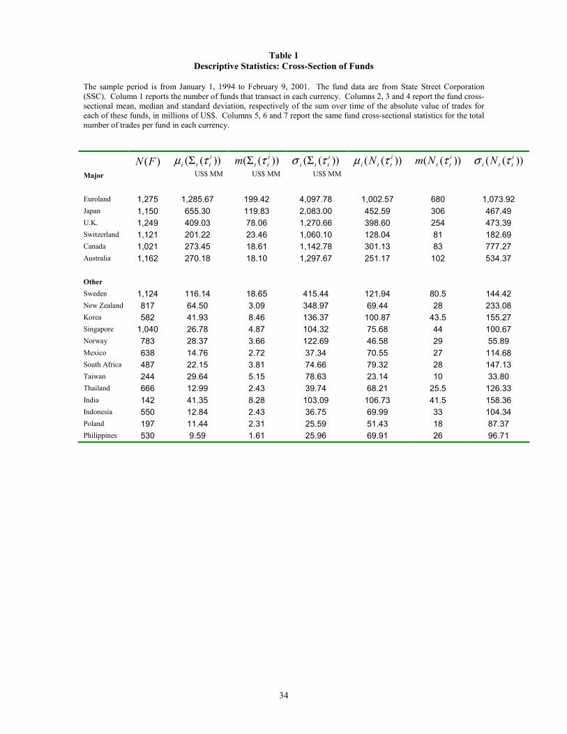
34

Table 1 Descriptive Statistics: Cross-Section of Funds

The sample period is from January 1, 1994 to February 9, 2001. The fund data are from State Street Corporation (SSC). Column 1 reports the number of funds that transact in each currency. Columns 2, 3 and 4 report the fund cross-sectional mean, median and standard deviation, respectively of the sum over time of the absolute value of trades for each of these funds, in millions of US$. Columns 5, 6 and 7 report the same fund cross-sectional statistics for the total number of trades per fund in each currency.

)(FN ))(( itti τµ Σ ))(( i

ttm τΣ ))(( itti τσ Σ ))(( i

tti N τµ ))(( ittNm τ ))(( i

tti N τσ

Major US$ MM US$ MM US$ MM Euroland 1,275 1,285.67 199.42 4,097.78 1,002.57 680 1,073.92 Japan 1,150 655.30 119.83 2,083.00 452.59 306 467.49 U.K. 1,249 409.03 78.06 1,270.66 398.60 254 473.39 Switzerland 1,121 201.22 23.46 1,060.10 128.04 81 182.69 Canada 1,021 273.45 18.61 1,142.78 301.13 83 777.27 Australia 1,162 270.18 18.10 1,297.67 251.17 102 534.37 Other Sweden 1,124 116.14 18.65 415.44 121.94 80.5 144.42 New Zealand 817 64.50 3.09 348.97 69.44 28 233.08 Korea 582 41.93 8.46 136.37 100.87 43.5 155.27 Singapore 1,040 26.78 4.87 104.32 75.68 44 100.67 Norway 783 28.37 3.66 122.69 46.58 29 55.89 Mexico 638 14.76 2.72 37.34 70.55 27 114.68 South Africa 487 22.15 3.81 74.66 79.32 28 147.13 Taiwan 244 29.64 5.15 78.63 23.14 10 33.80 Thailand 666 12.99 2.43 39.74 68.21 25.5 126.33 India 142 41.35 8.28 103.09 106.73 41.5 158.36 Indonesia 550 12.84 2.43 36.75 69.99 33 104.34 Poland 197 11.44 2.31 25.59 51.43 18 87.37 Philippines 530 9.59 1.61 25.96 69.91 26 96.71

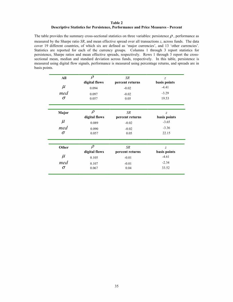
35

Table 2 Descriptive Statistics for Persistence, Performance and Price Measures - Percent

The table provides the summary cross-sectional statistics on three variables: persistence ρ , performance as measured by the Sharpe ratio SR, and mean effective spread over all transactions z, across funds. The data cover 19 different countries, of which six are defined as ‘major currencies’, and 13 ‘other currencies’. Statistics are reported for each of the currency groups. Columns 1 through 3 report statistics for persistence, Sharpe ratios and mean effective spreads, respectively. Rows 1 through 3 report the cross-sectional mean, median and standard deviation across funds, respectively. In this table, persistence is measured using digital flow signals, performance is measured using percentage returns, and spreads are in basis points.

All ρ SR z digital flows percent returns basis points

µ 0.094 -0.02 -4.41

med 0.097 -0.02 -3.29 σ 0.057 0.05 19.53

Major ρ SR z digital flows percent returns basis points

µ 0.089 -0.02 -3.65

med 0.090 -0.02 -3.36 σ 0.057 0.05 22.15

Other ρ SR z digital flows percent returns basis points

µ 0.105 -0.01 -4.61

med 0.107 -0.01 -2.34 σ 0.067 0.04 33.52

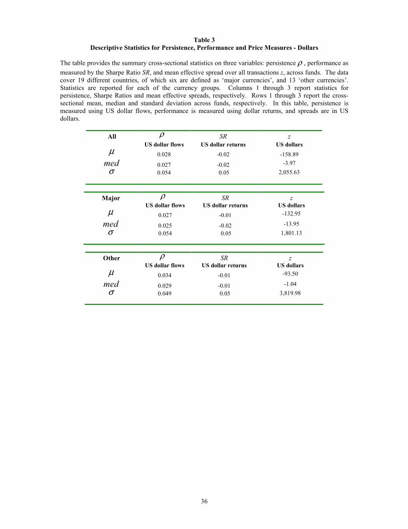
36

Table 3 Descriptive Statistics for Persistence, Performance and Price Measures - Dollars

The table provides the summary cross-sectional statistics on three variables: persistence ρ , performance as measured by the Sharpe Ratio SR, and mean effective spread over all transactions z, across funds. The data cover 19 different countries, of which six are defined as ‘major currencies’, and 13 ‘other currencies’. Statistics are reported for each of the currency groups. Columns 1 through 3 report statistics for persistence, Sharpe Ratios and mean effective spreads, respectively. Rows 1 through 3 report the cross-sectional mean, median and standard deviation across funds, respectively. In this table, persistence is measured using US dollar flows, performance is measured using dollar returns, and spreads are in US dollars.

All ρ SR z US dollar flows US dollar returns US dollars

µ 0.028 -0.02 -158.89 med 0.027 -0.02 -3.97

σ 0.054 0.05 2,055.63

Major ρ SR z

US dollar flows US dollar returns US dollars µ 0.027 -0.01 -132.95

med 0.025 -0.02 -13.95 σ 0.054 0.05 1,801.13

Other ρ SR z US dollar flows US dollar returns US dollars

µ 0.034 -0.01 -93.50

med 0.029 -0.01 -1.04 σ 0.049 0.05 3,819.98

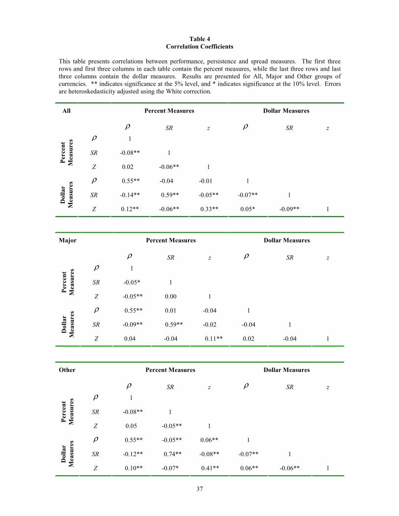
37

Table 4 Correlation Coefficients

This table presents correlations between performance, persistence and spread measures. The first three rows and first three columns in each table contain the percent measures, while the last three rows and last three columns contain the dollar measures. Results are presented for All, Major and Other groups of currencies. ** indicates significance at the 5% level, and * indicates significance at the 10% level. Errors are heteroskedasticity adjusted using the White correction.

All Percent Measures Dollar Measures

ρ SR z ρ SR z ρ 1

SR -0.08** 1

Perc

ent

Mea

sure

s

Z 0.02 -0.06** 1

ρ 0.55** -0.04 -0.01 1

SR -0.14** 0.59** -0.05** -0.07** 1

Dol

lar

Mea

sure

s

Z 0.12** -0.06** 0.33** 0.05* -0.09** 1

Major Percent Measures Dollar Measures

ρ SR z ρ SR z ρ 1

SR -0.05* 1

Perc

ent

Mea

sure

s

Z -0.05** 0.00 1

ρ 0.55** 0.01 -0.04 1

SR -0.09** 0.59** -0.02 -0.04 1

Dol

lar

Mea

sure

s

Z 0.04 -0.04 0.11** 0.02 -0.04 1

Other Percent Measures Dollar Measures

ρ SR z ρ SR z ρ 1

SR -0.08** 1

Perc

ent

Mea

sure

s

Z 0.05 -0.05** 1

ρ 0.55** -0.05** 0.06** 1

SR -0.12** 0.74** -0.08** -0.07** 1

Dol

lar

Mea

sure

s

Z 0.10** -0.07* 0.41** 0.06** -0.06** 1

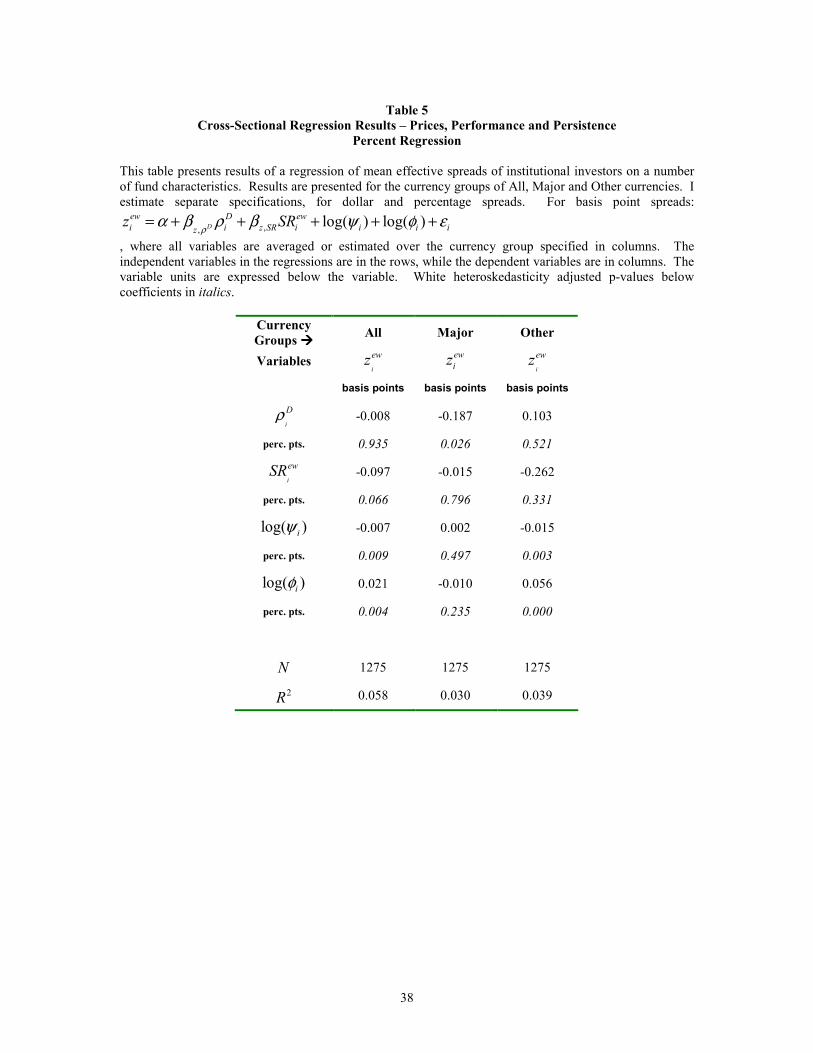
38

Table 5 Cross-Sectional Regression Results – Prices, Performance and Persistence

Percent Regression This table presents results of a regression of mean effective spreads of institutional investors on a number of fund characteristics. Results are presented for the currency groups of All, Major and Other currencies. I estimate separate specifications, for dollar and percentage spreads. For basis point spreads:

,,log( ) log( )D

ew D ewi i z SR i i i iz

z SRρ

α β ρ β ψ φ ε= + + + + +

, where all variables are averaged or estimated over the currency group specified in columns. The independent variables in the regressions are in the rows, while the dependent variables are in columns. The variable units are expressed below the variable. White heteroskedasticity adjusted p-values below coefficients in italics.

Currency Groups All Major Other

Variables i

ewz ewiz

i

ewz

basis points basis points basis points

i

Dρ -0.008 -0.187 0.103

perc. pts. 0.935 0.026 0.521

i

ewSR -0.097 -0.015 -0.262

perc. pts. 0.066 0.796 0.331

log( )iψ -0.007 0.002 -0.015

perc. pts. 0.009 0.497 0.003

log( )iφ 0.021 -0.010 0.056

perc. pts. 0.004 0.235 0.000

N 1275 1275 1275

2R 0.058 0.030 0.039

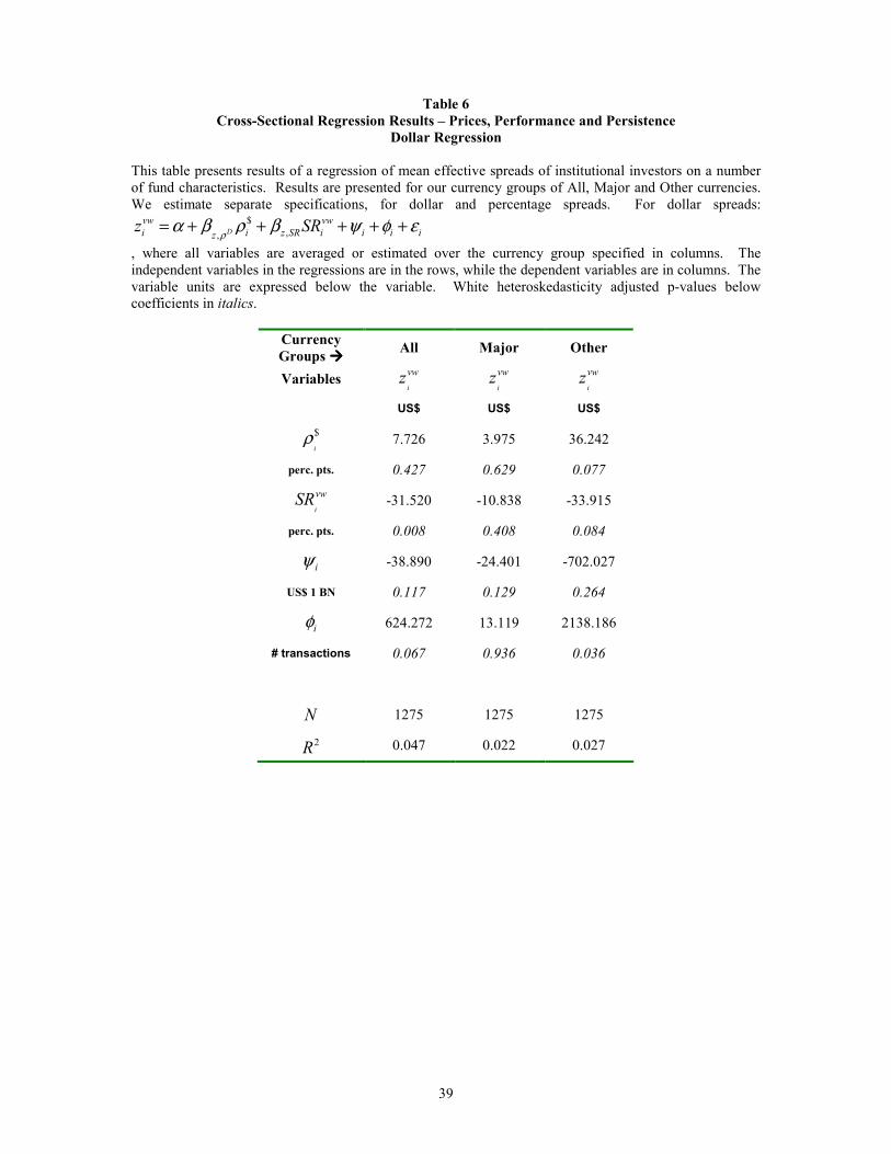
39

Table 6

Cross-Sectional Regression Results – Prices, Performance and Persistence Dollar Regression

This table presents results of a regression of mean effective spreads of institutional investors on a number of fund characteristics. Results are presented for our currency groups of All, Major and Other currencies. We estimate separate specifications, for dollar and percentage spreads. For dollar spreads:

$,, D

vw vwi i z SR i i i iz

z SRρ

α β ρ β ψ φ ε= + + + + +

, where all variables are averaged or estimated over the currency group specified in columns. The independent variables in the regressions are in the rows, while the dependent variables are in columns. The variable units are expressed below the variable. White heteroskedasticity adjusted p-values below coefficients in italics.

Currency Groups All Major Other

Variables i

vwz i

vwz i

vwz

US$ US$ US$

$i

ρ 7.726 3.975 36.242

perc. pts. 0.427 0.629 0.077

i

vwSR -31.520 -10.838 -33.915

perc. pts. 0.008 0.408 0.084

iψ -38.890 -24.401 -702.027

US$ 1 BN 0.117 0.129 0.264

iφ 624.272 13.119 2138.186

# transactions 0.067 0.936 0.036

N 1275 1275 1275

2R 0.047 0.022 0.027

40

Table 7 Panel Regression Results – Prices, Performance and Persistence

With Country-Specific Intercepts Percent Regression

This table presents results of a regression of mean effective spreads of institutional investors on a number of fund characteristics. Results are presented for the currency groups of All, Major and Other currencies. I estimate separate specifications, for dollar and percentage spreads. For basis point spreads:

, ,,log( ) log( )D

ew D ewi k k i z SR i i i iz

z SRρ

α β ρ β ψ φ ε= + + + + +

,where the dependent variable in all cases is the fund-currency stacked mean spread over all transactions in the pair. The independent variables in all cases are estimated over all transactions for each fund – the same regressors are used for all currencies. The independent variables in the regressions are in the rows, while the dependent variables are specified in columns. The variable units are expressed below the variables. White heteroskedasticity adjusted p-values below coefficients in italics.

Currency Groups All Major Other

Variables i

ewz ewiz

i

ewz

basis points basis points basis points

i

Dρ 0.123 -0.305 0.583

perc. pts. 0.261 0.000 0.005

i

ewSR -0.078 -0.050 -0.128

perc. pts. 0.111 0.221 0.190

log( )iψ -0.009 0.002 -0.021

perc. pts. 0.001 0.168 0.000

log( )iφ 0.011 0.001 0.006

perc. pts. 0.093 0.925 0.670

N 14781 6980 7801

2R 0.001 0.003 0.004

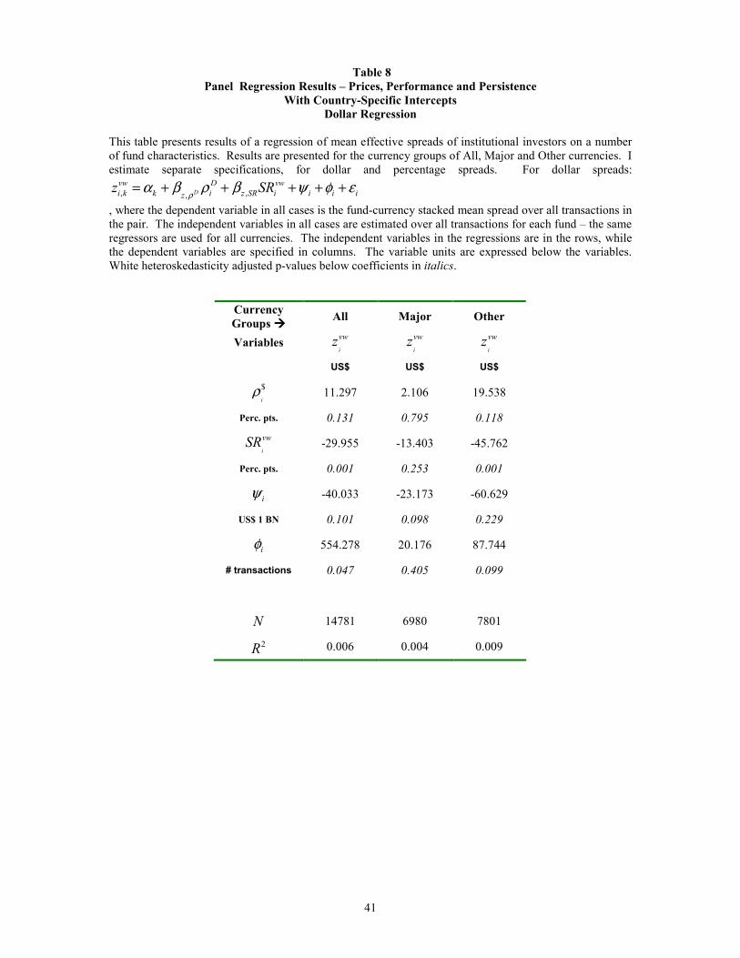
41

Table 8 Panel Regression Results – Prices, Performance and Persistence

With Country-Specific Intercepts Dollar Regression

This table presents results of a regression of mean effective spreads of institutional investors on a number of fund characteristics. Results are presented for the currency groups of All, Major and Other currencies. I estimate separate specifications, for dollar and percentage spreads. For dollar spreads:

, ,, Dvw D vwi k k i z SR i i i iz

z SRρ

α β ρ β ψ φ ε= + + + + +

, where the dependent variable in all cases is the fund-currency stacked mean spread over all transactions in the pair. The independent variables in all cases are estimated over all transactions for each fund – the same regressors are used for all currencies. The independent variables in the regressions are in the rows, while the dependent variables are specified in columns. The variable units are expressed below the variables. White heteroskedasticity adjusted p-values below coefficients in italics.

Currency Groups All Major Other

Variables i

vwz i

vwz i

vwz

US$ US$ US$

$i

ρ 11.297 2.106 19.538

Perc. pts. 0.131 0.795 0.118

i

vwSR -29.955 -13.403 -45.762

Perc. pts. 0.001 0.253 0.001

iψ -40.033 -23.173 -60.629

US$ 1 BN 0.101 0.098 0.229

iφ 554.278 20.176 87.744

# transactions 0.047 0.405 0.099

N 14781 6980 7801

2R 0.006 0.004 0.009

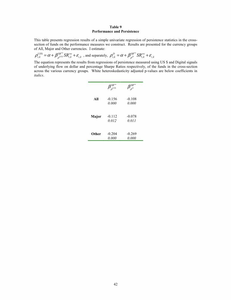
42

Table 9

Performance and Persistence

This table presents regression results of a simple univariate regression of persistence statistics in the cross-section of funds on the performance measures we construct. Results are presented for the currency groups of All, Major and Other currencies. I estimate:

$$

, , ,

vw

USUS SR vwi k i k i kSR

ρρ α β ε= + + , and separately, , , ,

ew

DD SR ewi k i k i kSR

ρρ α β ε= + +

The equation represents the results from regressions of persistence measured using US $ and Digital signals of underlying flow on dollar and percentage Sharpe Ratios respectively, of the funds in the cross-section across the various currency groups. White heteroskedasticity adjusted p-values are below coefficients in italics.

$

vw

USSRρβ

ew

DSRρβ

All -0.156 -0.108

0.000 0.000

Major -0.112 -0.078 0.012 0.011

Other -0.204 -0.269 0.000 0.000

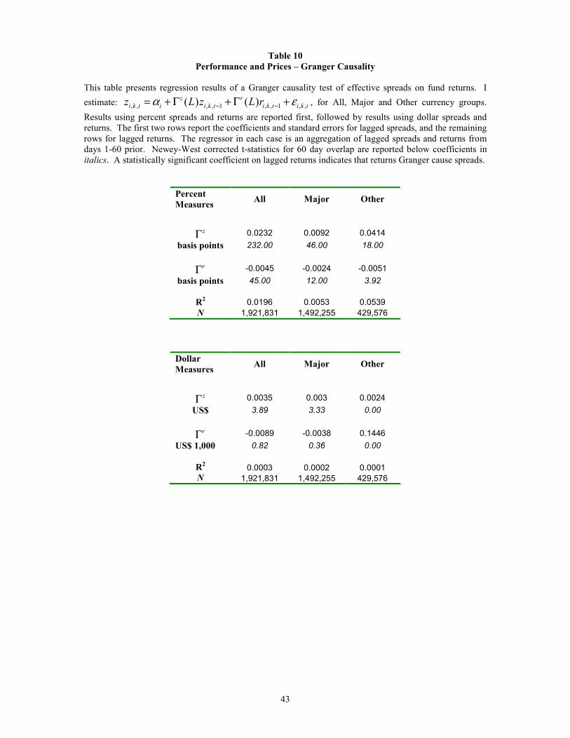
43

Table 10 Performance and Prices – Granger Causality

This table presents regression results of a Granger causality test of effective spreads on fund returns. I estimate: , , , , 1 , , 1 , ,( ) ( )z r

i k t i i k t i k t i k tz L z L rα ε− −= + Γ + Γ + , for All, Major and Other currency groups. Results using percent spreads and returns are reported first, followed by results using dollar spreads and returns. The first two rows report the coefficients and standard errors for lagged spreads, and the remaining rows for lagged returns. The regressor in each case is an aggregation of lagged spreads and returns from days 1-60 prior. Newey-West corrected t-statistics for 60 day overlap are reported below coefficients in italics. A statistically significant coefficient on lagged returns indicates that returns Granger cause spreads.

Percent Measures All Major Other

zΓ 0.0232 0.0092 0.0414

basis points 232.00 46.00 18.00

rΓ -0.0045 -0.0024 -0.0051 basis points 45.00 12.00 3.92

R2 0.0196 0.0053 0.0539 N 1,921,831 1,492,255 429,576

Dollar Measures All Major Other

zΓ 0.0035 0.003 0.0024

US$ 3.89 3.33 0.00

rΓ -0.0089 -0.0038 0.1446 US$ 1,000 0.82 0.36 0.00

R2 0.0003 0.0002 0.0001 N 1,921,831 1,492,255 429,576

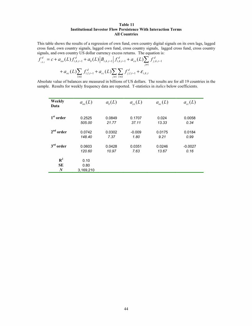
44

Table 11 Institutional Investor Flow Persistence With Interaction Terms

All Countries This table shows the results of a regression of own fund, own country digital signals on its own lags, lagged cross fund, own country signals, lagged own fund, cross country signals, lagged cross fund, cross country signals, and own country US dollar currency excess returns. The equation is:

, , , , 1 , , 1 , , 1 , , 1

, , 1 , , 1 , ,

( ) ( ) ( )

( ) ( )

i k t

d d d doo i k t b i k t i k t co j k t

j i

d doc i l t cc j l t i k t

l k j i l k

f c a L f a L B f a L f

a L f a L f ε

− − − −≠

− −≠ ≠ ≠

= + + +

+ + +

∑

∑ ∑∑

Absolute value of balances are measured in billions of US dollars. The results are for all 19 countries in the sample. Results for weekly frequency data are reported. T-statistics in italics below coefficients.

Weekly Data

( )ooa L ( )ba L ( )coa L ( )oca L ( )cca L

1st order 0.2525 0.0849 0.1707 0.024 0.0058

505.00 21.77 37.11 13.33 0.34 2nd order 0.0742 0.0302 -0.009 0.0175 0.0184 148.40 7.37 1.80 9.21 0.99

3rd order 0.0603 0.0428 0.0351 0.0246 -0.0027 120.60 10.97 7.63 13.67 0.16

R2 0.10 SE 0.80 N 3,169,210

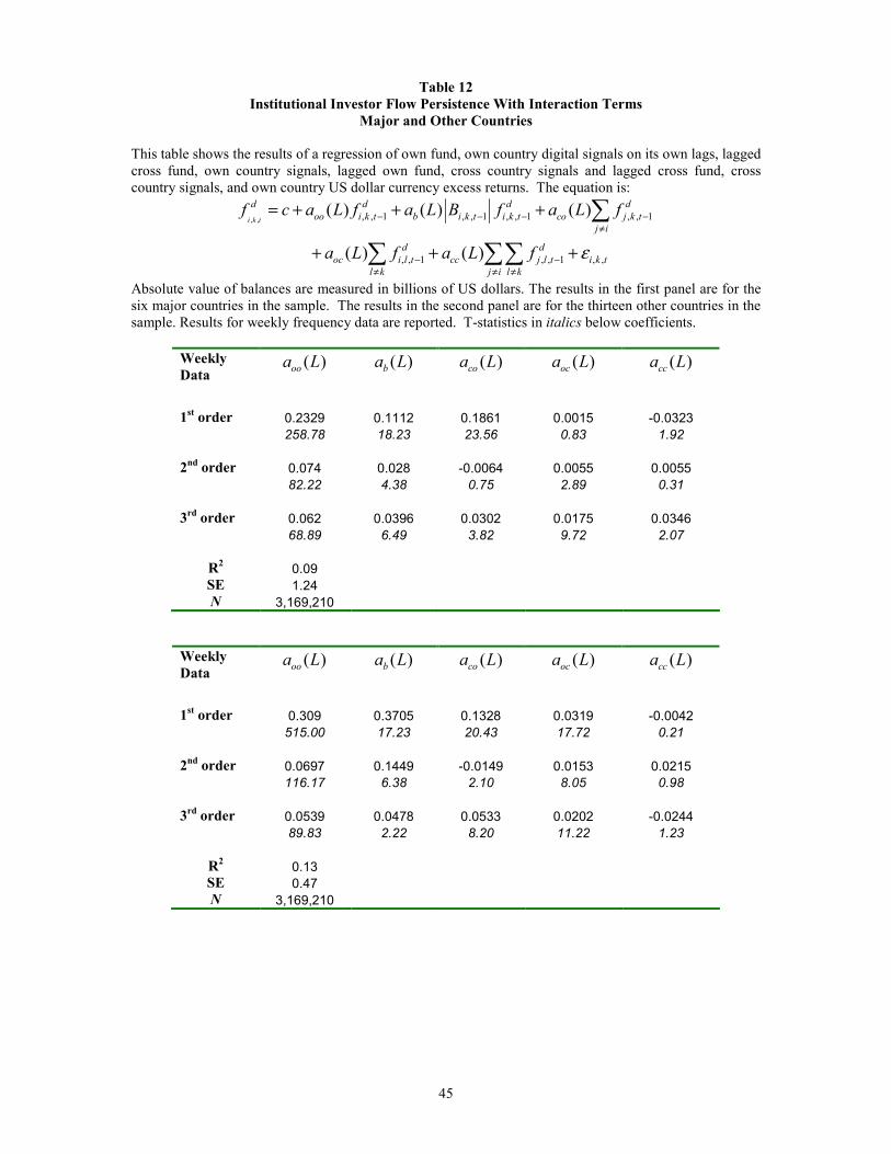
45

Table 12 Institutional Investor Flow Persistence With Interaction Terms

Major and Other Countries

This table shows the results of a regression of own fund, own country digital signals on its own lags, lagged cross fund, own country signals, lagged own fund, cross country signals and lagged cross fund, cross country signals, and own country US dollar currency excess returns. The equation is:

, , , , 1 , , 1 , , 1 , , 1

, , 1 , , 1 , ,

( ) ( ) ( )

( ) ( )

i k t

d d d doo i k t b i k t i k t co j k t

j i

d doc i l t cc j l t i k t

l k j i l k

f c a L f a L B f a L f

a L f a L f ε

− − − −≠

− −≠ ≠ ≠

= + + +

+ + +

∑

∑ ∑∑

Absolute value of balances are measured in billions of US dollars. The results in the first panel are for the six major countries in the sample. The results in the second panel are for the thirteen other countries in the sample. Results for weekly frequency data are reported. T-statistics in italics below coefficients.

Weekly Data

( )ooa L ( )ba L ( )coa L ( )oca L ( )cca L

1st order 0.2329 0.1112 0.1861 0.0015 -0.0323

258.78 18.23 23.56 0.83 1.92 2nd order 0.074 0.028 -0.0064 0.0055 0.0055 82.22 4.38 0.75 2.89 0.31

3rd order 0.062 0.0396 0.0302 0.0175 0.0346 68.89 6.49 3.82 9.72 2.07

R2 0.09 SE 1.24 N 3,169,210

Weekly Data

( )ooa L ( )ba L ( )coa L ( )oca L ( )cca L

1st order 0.309 0.3705 0.1328 0.0319 -0.0042

515.00 17.23 20.43 17.72 0.21 2nd order 0.0697 0.1449 -0.0149 0.0153 0.0215 116.17 6.38 2.10 8.05 0.98

3rd order 0.0539 0.0478 0.0533 0.0202 -0.0244 89.83 2.22 8.20 11.22 1.23

R2 0.13 SE 0.47 N 3,169,210