Permeation Barrier for Lightweight Liquid Hydrogen Tanks
159
Permeation Barrier for Lightweight Liquid Hydrogen Tanks Dissertation zur Erlangung des Doktorgrades der Mathematisch-Naturwissenschaftlichen Fakult¨ at der Universit¨ at Augsburg vorgelegt von Daniel Schultheiß 16. April 2007 OPUS Augsburg der Online-Publikationsserver der Universit¨ at Augsburg
Transcript of Permeation Barrier for Lightweight Liquid Hydrogen Tanks

Permeation Barrier for Lightweight
Liquid Hydrogen Tanks
Dissertation zur Erlangung des Doktorgradesder Mathematisch-Naturwissenschaftlichen Fakultat
der Universitat Augsburg
vorgelegt von
Daniel Schultheiß
16. April 2007
OPUS Augsburgder Online-Publikationsserver der Universitat Augsburg

Erstgutachter: Prof. Dr. Siegfried R. HornZweitgutachter: Prof. Dr. Ferdinand Haider
Tag der mundlichen Prufung: 06. Juni 2007

Contents
Table of Contents i
Notation iii
1 Introduction 1
2 Permeation in Metals and Polymers 72.1 Structure of Metals and Polymers . . . . . . . . . . . . . . . . . . . . . . . 72.2 Fundamental Equations . . . . . . . . . . . . . . . . . . . . . . . . . . . . 92.3 Sorption . . . . . . . . . . . . . . . . . . . . . . . . . . . . . . . . . . . . . 10
2.3.1 Modes of Sorption . . . . . . . . . . . . . . . . . . . . . . . . . . . 102.3.2 Sorption in Metals . . . . . . . . . . . . . . . . . . . . . . . . . . . 122.3.3 Sorption in Polymers . . . . . . . . . . . . . . . . . . . . . . . . . . 132.3.4 General Sorption Equation . . . . . . . . . . . . . . . . . . . . . . . 14
2.4 Diffusion . . . . . . . . . . . . . . . . . . . . . . . . . . . . . . . . . . . . . 142.4.1 Phenomenological Description . . . . . . . . . . . . . . . . . . . . . 142.4.2 Atomistic Description . . . . . . . . . . . . . . . . . . . . . . . . . 162.4.3 Solution of Fick’s Laws . . . . . . . . . . . . . . . . . . . . . . . . . 182.4.4 Grain Boundary Diffusion . . . . . . . . . . . . . . . . . . . . . . . 19
2.5 Permeation . . . . . . . . . . . . . . . . . . . . . . . . . . . . . . . . . . . 222.5.1 Phenomenological Description . . . . . . . . . . . . . . . . . . . . . 222.5.2 Experimental Determination of P and D . . . . . . . . . . . . . . . 232.5.3 Serial and Parallel Permeation . . . . . . . . . . . . . . . . . . . . . 262.5.4 Permeation through Substrates with Defective Liners . . . . . . . . 282.5.5 Comparison of Hydrogen and Helium Permeation . . . . . . . . . . 30
2.6 Simulation of Permeation . . . . . . . . . . . . . . . . . . . . . . . . . . . . 31
3 Preselection of Feasible Liner Materials and Production Processes 393.1 Literature Review of LH2 Tank Liners . . . . . . . . . . . . . . . . . . . . 393.2 Literature Review of Hydrogen Permeabilities . . . . . . . . . . . . . . . . 413.3 Outgassing and Literature Review of Outgassing Rates . . . . . . . . . . . 423.4 Vacuum Stability and Material Preselection . . . . . . . . . . . . . . . . . 443.5 Literature Review and Preselection of Liner Production Processes . . . . . 46
i

4 Materials 514.1 Substrates . . . . . . . . . . . . . . . . . . . . . . . . . . . . . . . . . . . . 514.2 Liners . . . . . . . . . . . . . . . . . . . . . . . . . . . . . . . . . . . . . . 534.3 Specimens . . . . . . . . . . . . . . . . . . . . . . . . . . . . . . . . . . . . 60
5 Measurement of Permeation 615.1 Room Temperature Permeation Measurement Apparatus . . . . . . . . . . 61
5.1.1 Test Set-up . . . . . . . . . . . . . . . . . . . . . . . . . . . . . . . 615.1.2 Test Procedure . . . . . . . . . . . . . . . . . . . . . . . . . . . . . 635.1.3 Calibration . . . . . . . . . . . . . . . . . . . . . . . . . . . . . . . 65
5.2 Cryogenic Permeation Measurement Apparatus . . . . . . . . . . . . . . . 675.3 Evaluation and Error Estimation . . . . . . . . . . . . . . . . . . . . . . . 71
6 Results and Discussion 736.1 Initial Permeation Tests . . . . . . . . . . . . . . . . . . . . . . . . . . . . 73
6.1.1 Reliability of the Measurement Apparatuses . . . . . . . . . . . . . 736.1.2 Comparison of Hydrogen and Helium Permeation . . . . . . . . . . 766.1.3 Influence of the Feed Pressure . . . . . . . . . . . . . . . . . . . . . 806.1.4 Influence of Thermal Cycling . . . . . . . . . . . . . . . . . . . . . 81
6.2 Results of the Permeation Measurements . . . . . . . . . . . . . . . . . . . 826.2.1 CFRP Substrates . . . . . . . . . . . . . . . . . . . . . . . . . . . . 826.2.2 Metal Sheets and Foils . . . . . . . . . . . . . . . . . . . . . . . . . 836.2.3 Metal-plated CFRP . . . . . . . . . . . . . . . . . . . . . . . . . . . 856.2.4 Miscellaneous Coatings on CFRP . . . . . . . . . . . . . . . . . . . 89
6.3 Simulation of Transient Permeation . . . . . . . . . . . . . . . . . . . . . . 906.3.1 Simulation of Grain Boundary Diffusion . . . . . . . . . . . . . . . 906.3.2 Simulation of Two-layer Permeation . . . . . . . . . . . . . . . . . . 916.3.3 Simulation of Permeation through Substrates with Defective Liner . 95
6.4 Discussion . . . . . . . . . . . . . . . . . . . . . . . . . . . . . . . . . . . . 976.4.1 Permeation through CFRP . . . . . . . . . . . . . . . . . . . . . . . 976.4.2 Permeation through Metal-plated CFRP . . . . . . . . . . . . . . . 986.4.3 Evaluation of the Barrier Function of the Liners . . . . . . . . . . . 103
7 Conclusions 105
A Literature Survey of H2 Permeabilities 111
B Literature Survey of Outgassing Rates 123
C List of Materials 129
D Measured Data 133
Bibliography 137
ii

Notation
List of frequently used symbols
a lattice constantb widthd diameter of the sealing ringj normalized fluxl thicknessm massn pressure exponent (sorption)p pressure (general)pf, pp pressure at feed/permeate sideps vapor saturation pressureqG area specific outgassing rater defect radiuss pumping speedseff effective pumping speedt timex coordinate
A areaC concentrationCf, Cp C at the feed/permeate sideD diffusivityD0 pre-exponential factor of DEa activation energy (general)ED, EP, ES activation energy of D, P , SJ fluxJss steady-state fluxM molar massN number of particle in molP permeability
P0 pre-exponential factor of PQ gas flowQG outgassing rateQL leak rateQP permeation gas flowQT throughputR universal gas constant (mostly
in the form of RT )R defect separation distanceS solubility, Henry’s constantS0 pre-exponential factor of SSS solubility, Sievert’s constantT temperatureTmc T of the measuring chamberTg glass transition temperatureV volume
ι barrier constantµ chemical potentialµ0 standard chemical potential at
standard conditionsνf fractional free volumeτ dimensionless time
SubscriptsG grainB grain boundarys substratel liner
iii

List of Abbreviations and Acronyms
bcc body-centered cubiccAu chemical goldcCu chemical coppercNiP chemical nickel phosphorfcc face-centered cubichcp hexagonal close-packed
CFRP carbon fiber reinforced plasticCPMA cryogenic permeation
measurement apparatusDLC diamond-like carbonEDX energy dispersive x-rayFDM finite difference methodLH2 liquid hydrogenLHe liquid heliumLN2 liquid nitrogenM01, ... material system numberPVD physical vapor depositionQMS quadrupole mass spectrometerRT room temperatureRTPMA room temperature permeation
measurement apparatusS01, ... specimen number
SEM scanning electron microscopyUHV ultra high vacuum
ECTFE ethylen/chlortrifluorethylenHDPE high density polyethyleneInconel austenitic nickel-based alloyKovar nickel-cobalt ferrous alloyLDPE low density polyethyleneMonel nickel copper iron alloyMylar see PETPPA polyamidePBO polyphenylene oxidePC polycarbonatePE polyethylenePETP PolyethylenterephthalatPI polyimidePP polypropylenePTFE polytetrafluoroethylenePU polyurethanePVC polyvinyl chlorideSS stainless steelTeflon see PTFEVdC vinylidenchloride
Abbreviation List of Company Names
C01 BMW GroupC02 Oerlikon Space AGC03 Institut fur Verbundwerkstoffe GmbHC04 AIMT Holding GmbHC05 Luberg Elektronik GmbH & Co. Rothfischer KGC06 Aluminal Oberflachentechnik GmbH & Co. KGC07 Leistner GmbHC08 OMT – Oberflachen- und Materialtechnologie GmbHC09 Universitat Augsburg, Institut fur PhysikC10 MT Aerospace AGC11 Magna Steyr Space TechnologyC12 Linde AGC13 Alfa Aesar GmbH & Co. KGC14 Roth GmbH
iv

Chapter 1
Introduction
Conventional fossil energy sources like coal, oil and natural gas are only time-limited avail-able [1–11]. Additionally, the emission of carbon dioxide owing to the combustion of fossilenergy sources is made responsible for the increasing greenhouse effect and therefore forthe global warming [12–15]. Hydrogen (H2) is an alternative energy carrier that does notcontain carbon. Its usage as a fuel in automobiles is the subject of recent research anddevelopment. Thereby, the storage of H2 on board is an essential issue. One technicalsolution is the storage of liquefied hydrogen (20K, 1 – 6 bar) in vacuum insulated tankvessels. Liquid hydrogen (LH2) tanks made of carbon fiber reinforced plastics (CFRP) areof special interest because they enable lightweight structures. However, the permeation ofhydrogen through CFRP, a potential source of deteriorating the vacuum, is still a challengeto be solved.
Automotive LH2 Tank and its Vacuum Insulation
The minimization of arbitrary heat fluxes into the liquid hydrogen is one of the key issueswhen developing a LH2 tank. Heat transfer leads to an evaporation and hence to a lossof hydrogen. Vacuum insulations, as employed in thermo flasks, provide the most efficientprotection.
Figure 1.1 illustrates the LH2 tank of the BMW Hydrogen 7. Concerning the storagefunction, the main parts of the system are the inner and the outer tank vessel, and thein-between superinsulation. Further parts are explained within the figure. The superinsu-lation consists of an evacuated space in combination with multi-layer foils, see figure 1.2.The vacuum between the inner and the outer tank vessel enables a reduction of the con-vection and thermal conduction. The multi-layer foils are added to reduce the radiation.Compared to other insulation methods, the superinsulation is advantageous because of itsvery low thermal conductivity1.
Figure 1.3 emphasizes the importance of high vacuum within the superinsulation. Thethermal conductivity of the superinsulation is plotted as a function of the vacuum pres-sure. Exceeding 10−3 mbar, the thermal conductivity increases rapidly. At 0.3mbar, theinsulation is deteriorated by factor 200.
The main factors that can deteriorate the insulating vacuum are schematically shownin figure 1.4. These five factors can be categorized into three processes: gas permeation,
1The thermal conductivity of the superinsulation is approximately 3 ·10−5 W/mK. For comparison, thethermal conductivity of polystyrene (Styrofoam) is between 3 · 10−3 W/mK at very low temperatures and1.5W/mK at room temperature [16].
1

2 1 Introduction
Figure 1.1: X-ray view of the LH2 tankof the Hydrogen 7. The tank consists of aninner and an outer tank, enclosing an insu-lating vacuum. The inner tank contains thestored hydrogen as well as filling and extrac-tion pipes, an evaporator and a level gauge.The inner tank is suspended from the outertank at the polar caps. The auxiliary boxoutside the tank hosts, among other things,valves and a heat exchanger. Source: MagnaSteyr.
LH2
inner tank
foils
vacuum
outer tank
Figure 1.2: Schematic sectionof a LH2 tank. The inner tankstores the liquid hydrogen. Itis surrounded by the superinsu-lation consisting of vacuum andmulti-layer foils. The inner tankand the insulation are hosted bythe outer tank. Suspensions,pipes, valves, etc. are not drawn.
10-5 10-4 10-3 10-2 10-110-5
10-4
10-3
10-2
ther
mal
con
duct
ivity
/ W
m-1 K
-1
p / mbar
Figure 1.3: Thermal conductivity of thesuperinsulation as a function of the vacuumpressure. The conductivity increases stronglyfor pressures greater than 10−3 mbar. From[17].

1 Introduction 3
H2 permeation
outgassing
outgassing
inner tank
through inner tank
outer tank
leaks
air permeationthrough outer tank
Figure 1.4: Main fac-tors that deteriorate thevacuum of the superinsula-tion. Influences of suspen-sions, pipes, valves, etc. arenot considered here.
outgassing and leakage. While definitions and detailed explanations of permeation andoutgassing are given in chapter 2 and 3, leakage is not further investigated.
Automotive Lightweight LH2 Tank
The state-of-the-art LH2 tank as described above is cylindrically shaped and made ofstainless steel (SS). Its mass without auxiliary system parts is approximately 100 kg, for10 kg stored LH2 [18]. The automotive industry would benefit from an optimized shape anda reduced weight of the tank. One objective of the European project StorHy (HydrogenStorage Systems for Automotive Application) is to present such a tank. More specific, thetank mass for a storage capacity of 10 kg LH2 shall be reduced from 100 kg to 30 kg. Thechosen tank design is depicted in figure 1.5. Although it reminds to the cylindrical shape,this storage system contains all necessary elements to realize a form-adapted design.
CFRP meets the demands of the new design and the weight reduction. Comparedto stainless steel, the weight-specific stiffness and strength of CFRP can be several timeshigher [19; 20]. Besides their advantageous mechanical properties, the design of CFRPscan be optimized to fulfill specific requirements like anisotropic loads — as existing in aLH2 vessel. On the other hand, CFRP is highly permeable to hydrogen and shows highoutgassing rates. Hence, a liner is required, that means a permeation and outgassing barrierto protect the vacuum.
Objective and Outline
The objective of this thesis is the development of an adequate protection (liner) againstH2 permeation through the inner vessel of a CFRP liquid hydrogen tank. The liner shalladditionally prevent the outgassing of the CFRP. Considering outgassing, a liner at theoutside of the inner tank is mandatory. To prevent permeation, the liner can be eitherapplied at one of both surfaces or inside the tank shell. The liners investigated in this workare only applied at the surface facing the vacuum, i. e. at the outside of the inner tank.

4 1 Introduction
(a) Inner Tank (b) Outer Tank
Figure 1.5: Design of the chosen lightweight LH2 tank concept. The inner tank contains atension sheet to suppress buckling of the cylindrical part as well as a tension bar to carry axialloads and enable flat polar caps. Though both elements would not be required for a cylindricaltank, they are mandatory for a free-form tank with concave-convex shapes. Hence, this innertank includes all parts to demonstrate the feasibility of a form-adapted design. The outer tankfollows the shape of the inner tank. A transformation to a form-adapted design can be realizedby adding stiffeners. Source: BMW Group Research and Technology.
The more specific objective of this work is to preselect and subsequently test suitableliner materials and the according production processes. Thereby, the main emphasis islaid on the evaluation of these liner materials and –production processes regarding theirpermeation performance.
Following this introductory chapter, chapter 2 gives an introduction to permeationthrough metals and polymers. Since it is important for understanding the different perme-ation processes, first the structure of metals and polymers is explained. After presentingequations to describe gases and their transport, the two subprocesses of permeation, sorp-tion and diffusion, are described. There, the modes of sorption, the differences betweensorption in metals and polymers, the atomistic and phenomenological description of diffu-sion, and the grain boundary diffusion are presented. In the following, the total permeationprocess is explained by introducing governing equations and material properties like thepermeability. Experimental methods are presented to determine those material proper-ties. Next, four modes of permeation are distinguished and explained: permeation througha homogeneous material, through parallel or serial materials, and through a defectivelycoated material. At the end of this chapter, a program to simulate transient permeationis presented. The objective of simulating transient permeation is to obtain characteristicshapes of the flux-time curve, depending on the mode of permeation.
In the third chapter, feasible liner materials and processes are reviewed, evaluated andpreselected. First, a literature survey is performed on liners applied or planned for LH2
tanks. Second, permeabilities and outgassing rates of different materials are reviewed fromthe literature. The review includes a large number of publications to enable a meaningful

1 Introduction 5
selection. Third, the required liner permeability and outgassing rate to enable a stable tankvacuum are assessed by performing a sample calculation. Considering both permeation andoutgassing, a metallic liner is mandatory to sustain a stable insulating tank vacuum. Fea-sible processes to produce metallic liners are presented in the following. Considering theproducibility on CFRP, the preselected liner production processes are metal plating2, ad-hesion of foils, thermal spraying and physical vapor deposition. The investigated materialsinclude aluminum, copper, gold, nickel, tin and additionally diamond-like carbon.
The next chapter 4 presents and characterizes the selected materials. ConsideringCFRP and particularly the liners, their basic properties like thermal shock resistance,adhesive strength, structure and potential material defects are discussed. SEM imagesof the surface and the section of the liners give information about grain-like structures,thickness distribution or the formation of cracks. At the end of this chapter, the size andshape of the utilized specimens are illustrated. A list of all specimens summarizing theirproperties and production details is presented in appendix C.
Chapter 5 describes the measurement of permeation. Two apparatuses are employedworking from 20K to 293K, and from 293K to 373K respectively. The set-up of bothapparatuses is presented and explained. A typical test procedure is exemplarily describedin the following section. Because a main focus is laid on high-quality results, the calibrationof the experimental set-up is discussed. The last part of this chapter explains the evaluationof the measurements and estimates the maximum experimental error.
In chapter 6, the results of the permeation measurements and simulations are presented,compared and discussed. First, initial tests to verify the reliability of the measurementsare performed. Second, the permeation of hydrogen and helium through eleven specimensis compared. Since the permeation performances of both gases are similar and hydrogen isdisadvantageous owing to its higher minimum detection limit, it is concluded to use heliumas test gas in the following. Third, the influence of the feed pressure and of thermal shockson the permeability of selected specimens is determined. The following section 6.2 liststhe results of the permeation measurements on all specimens. Besides the presentationof the permeabilities, information about the activation energy, diffusivity and the shapeof the flux-time is given. In 6.3, the results of the simulations of permeation thoughparallel grain boundaries, through serial materials and through materials with defectiveliners are presented. Both, the results of the measurements and simulations are comparedand discussed in 6.4. In particular, the mode of permeation through CFRP and throughmetal-plated CFRP is determined. Finally, the results of the permeation measurementsare evaluated together with the material characterization of chapter 4. A recommendationfor suitable liners is given.
The last chapter summarized this thesis and gives an outlook on future work.
2Throughout this thesis, metal plating denotes the generic term for electroless plating and electroplating.

6 1 Introduction

Chapter 2
Permeation in Metals and Polymers
“A theory is something nobody believes, except theperson who made it . . . ” continued on page 61
This chapter gives a detailed description of permeation in metals and polymers. First,the structure of these materials is explained and fundamental equations to describe gasesand their transport are presented. The next two sections deal with sorption and diffu-sion, the subprocesses of permeation. The permeation process itself is treated afterwards.Finally, the developed program to simulate permeation is presented.
2.1 Structure of Metals and Polymers
The mechanism and the rate of permeation are strongly related to the structure of thebulk material. While metals and metal alloys are characterized by their compact crystalstructure, polymers are amorphous.
The three types of crystal structure in metals, face-centered cubic (fcc), body-centeredcubic (bcc) and hexagonal close-packed (hcp), are shown in figure 2.1. Table 2.1 summarizesthe lattice types and the according lattice constants of selected metals. The structure of atrue metal, however, is a crystal containing imperfections. Common defects are vacancy orinterstitialcy (point defects), edge or screw dislocation (line defects) and grain boundaries(planar defects).
The common feature of all polymers is the co-existence of molecule chains and freevolumes [23–26]. The noncrystalline structures of polymers are less tightly packed thanmetals. Depending on the cross-linkage of the chains one distinguishes between thermo-plastics, thermosets and elastomers. In this thesis, only thermosets and thermoplastics arefurther considered and illustrated in figure 2.2. Thermoplastics consist of linear or lessbranched but not cross-linked chains. The bonding between the chains are owing to van-der-Waals or hydrogen-bridge forces. The polymer chains of thermosets, on the contrary,
Table 2.1: Crystal structure of some metals. The lattice constant a is taken from [22].
lattice metals a / Afcc copper, silver, gold, platinum, aluminum, nickel, lead, palladium 3.52 – 4.95bcc iron, vanadium, niobium, tantalum, molybdenum, tungsten 2.87 – 3.31hcp titanium, zinc 2.67 – 2.95
7

8 2 Permeation in Metals and Polymers
(a) fcc (b) bcc (c) hcp
Figure 2.1: The three lattice types of metals. The atomic packing factor of fcc, bcc and hcplattices is 0.74, 0.68 and 0.74, respectively [21].
(a) thermoset (b) amorphous thermoplastic (c) semi-crystalline thermoplastic
Figure 2.2: Molecular structure of thermosets and thermoplastics. Thermosets contain strongcovalent bindings between the molecular chains. Thermoplastics form weak van-der-Waals orhydrogen-bridge bindings. Depending on the structure of the chains, one defines amorphous andsemi-crystalline thermoplastics. The space not occupied by the molecule chains is called freevolume.

2.2 Fundamental Equations 9
are strongly cross-linked to form a net. The existing covalent forces are much stronger thanthe cohesion forces of thermoplastics.
Free volumes (also: microcavities, holes) exist in both polymer classes. Their size isfew Angstroms [27]. They are permanently formed and destroyed caused by oscillations ofthe macromolecular chains. The oscillations as well as the number of holes increase withincreasing temperature. Additionally, the number of holes is proportional to the grade ofcrystallinity [28; 29]. To quantify the free volumes, the fractional free volume is introducedwhich is defined by
νf =Vf
Vtot
, (2.1)
where Vf is the volume not occupied by chains and Vtot is the total volume.The properties of polymers are strongly temperature-dependent. With increasing tem-
perature, the chains of thermoplastics contain enough energy to enable rotation aroundthe single C–C bindings. At the glass transition temperature, Tg, the material becomessoft. A further increase of the temperature leads to overcoming the inter-chain forces andresults in melting. Thermosets, on the contrary, do not melt. Breaking apart the covalentforces, the thermoset splits into smaller parts and carbonizes. This characteristic distin-guishes thermoplastics from thermosets. While thermoplastics can be repeatedly heatedand formed, thermosets can only be once heated and formed.
Epoxy resins are one class of thermosets. The bindings of the epoxy groups are relativelystrong and result in very stable materials. Because of their advantageous properties theyare used as adhesives or matrices of composites.
2.2 Fundamental Equations
The behavior of gases in HV (high vacuum, 10−7 mbar – 10−3 mbar) and UHV (ultra-highvacuum, < 10−7 mbar) can be described by the state equation of ideal gases
p V = NRT, (2.2)
where p is the pressure, V is the volume, N is the number of particle in mol, R is theuniversal gas constant, and T is the absolute temperature. The transport of gases isgenerally quantified by the gas flow
Q =d (p V )
dt, (2.3)
where t is the time. The gas flow is per definition an energy flow. The energy expressionp V is called gas amount. Depending on the origin of the gas flow, it can be classified intothe leak rate (QL), outgassing rate (QG), permeation gas flow (QP), or throughput (QT).The throughput is the rate of pumping and is defined as
QT = s p, (2.4)

10 2 Permeation in Metals and Polymers
NA
Figure 2.3: Definition of the flux J . The amount of particles dNcrosses the area A in time dt.
where s is the pumping speed and p is the pressure at the inlet of the pump. In manyapplications, the area specific gas flow is used to describe transport processes:
q = Q/A, (2.5)
where A is the area.The transport of gases in permeation processes is usually described by the flux, J . The
flux is defined as the rate of particles per unit area, see figure 2.3
J =1
A
dN
dt. (2.6)
Substituting (2.2) and (2.3) in (2.6), the relationship between the flux and the gas flow is
J =1
ARTQ. (2.7)
The flux can also be expressed by the concentration flow. The concentration of amaterial is defined as the number of particles dN per occupied volume dV :
C =dN
dV. (2.8)
Substituting (2.8) in (2.6) and considering dV/dt = Adx/dt = Av, where v is the averagevelocity of the particles, one obtains
J = C v. (2.9)
2.3 Sorption
2.3.1 Modes of Sorption
Sorption is the general term for all interactions at surfaces between molecules of two phases.In this thesis, only the interactions between molecules of the gas phase (solute) and thesurface of a solid (solvent) are considered.
If molecules of the gas phase hit the surface of a solid, they can stick on it with acertain probability. This process is called adsorption. Depending on the existing cohesionforces, one defines physisorption (van-der-Waals forces) and chemisorption (covalent bondforces). The molar sorption energy of physisorption and chemisorption are approximately

2.3 Sorption 11
30 kJ/mol and 500 kJ/mol, respectively [30; 31]. Desorption is the opposite process ofadsorption. Absorption denotes the migration of the solutes into the bulk of the solvent.
Adsorption can be classified into mono-layer and multi-layer adsorption. Mono-layeradsorption is typically described by the Langmuir model [32]. There, only one layer ofgas atoms/molecules can stick on the surface of the solvent. The coverage grade, θ, isdefined for values between 0 (no adsorbed atoms) and 1 (surface is totally covered by onelayer of solutes). Additionally, Langmuir presumed that the solutes do no react with eachother. Hence, the adsorption rate or the sticking probability, respectively, is proportionalto 1 − θ. The desorption rate is proportional to θ exp [−Ea/RT ]. The Boltzmann factor,exp [−Ea/RT ], is typical for thermally activated process. It expresses the probability ofone atom or molecule accumulating the additional energy Ea to overcome a barrier [33].In equilibrium of adsorption and desorption, the according rates are equal and one obtainsthe Langmuir isotherm
θ =B p
1 +B p, (2.10)
where θ is the surface coverage factor, B = B0 exp [−EB/RT ] is a temperature-dependentmaterial constant reflecting the bond strength of the solute, and p is the pressure in thegas phase.
Multi-layer adsorption reflects the ability of solutes to stick on already adsorbed solutelayers. While mono-layers are physisorbed or chemisorbed, the following layers are con-densed gases [30]. Brauner, Emmett and Teller (BET) have developed a model to describethis process. They presumed, that the next layer can only grow if the underlying layer isfully covered. Hence, the adsorption rate is again proportional to 1 − θ. The desorptionprocess follows the laws of evaporation. The derived surface coverage factor is describedby the BET isotherm [30]
θ =rBET p
(ps − p) [1 + (rBET − 1) p/ps], (2.11)
where rBET is the ratio of the sticking times of adsorption and condensation layer, p is thegas pressure, ps is the vapor saturation pressure.
Considering θ ∝ C, the Langmuir isotherm (2.10) and the BET isotherm (2.11) can bemodified respectively to
C =S∗B p
1 +B pand C =
S∗∗ rBET p
(ps − p) [1 + (rBET − 1) p/ps], (2.12)
where S∗ and S∗∗ are material constants. Both isotherms describe the dependency ofthe surface concentration on the pressure at a constant temperature. The functions areschematically plotted in figure 2.4-b and -d, respectively. The Langmuir isotherm ap-proaches a horizontal asymptote for p → ∞. Similarly to the Langmuir-isotherm, theBET isotherm first converges a saturation region. Near the vapor saturation pressure, theconcentration becomes infinity.

12 2 Permeation in Metals and Polymers
conc
entr
atio
n
pressure
(a) Henry mode
conc
entr
atio
npressure
(b) Langmuir mode
conc
entr
atio
n
pressure
(c) Dual mode
conc
entr
atio
n
pressure
(d) BET mode
Figure 2.4: Sorption modes
In both models describing the mono-layer and the multi-layer adsorption, the concen-tration is direct proportional to the gas pressure for p→ 0. This behavior is expressed byHenry’s law:
C = S p, (2.13)
where S is called solubility or Henry’s constant. The Henry sorption mode is plotted infigure 2.4-a. The solubility includes the probability term for thermally activated processesand is mathematically expressed by the Arrhenius equation
S = S0 e−ES/R T , (2.14)
where S0 is a temperature-independent but gas-dependent material constant, and ES is theactivation energy of sorption.
The combination of the Henry and Langmuir isotherms is called Dual mode (see fig-ure 2.4-c). Its importance is described in 2.3.3.
2.3.2 Sorption in Metals
The adsorption of gases on metal surfaces can be physisorption or chemisorption. Accordingto Fromm [31], chemisorption is particularly present at active centers on the surface likedefects, grain boundaries, corners and edges. In general, the activities of the centerscan vary, i. e. the surface is energetically heterogeneous. Depending on the gas type, theadsorption process exhibits different behaviors. In particular, a difference is observedbetween one and two-atomic gases.
Several publications [31; 34–37] describe the absorption process of two-atomic gases likehydrogen. The molecules first adsorb physically on the surface. The molecules dissociatein a second step and become chemically adsorbed. The adsorbed gas atoms exchange theirsurface place with the first interstitial layers within the solid (absorption). These reactionsteps always exist in both directions, i. e. molecular adsorption counteracts desorption,surface dissociation counteracts recombination. The sum of the reaction steps lead toSievert’s law
C = SS
√p, (2.15)

2.3 Sorption 13
where SS is the solubility of the dissociative absorption or Sievert’s constant.The absorption process of one-atomic gases like helium in metals is rarely investigated.
The process is treated as a sequence of physisorption and movement from the surfaceto interstitial or vacancy sites within the solid [31]. The relationship between surfaceconcentration and gas pressure is commonly modeled by Henry’s law (2.13).
Equations (2.13) and (2.15) are valid as long as gases can be considered to be ideal andto follow equation (2.2). At high pressures and low temperatures, gases show a non-idealbehavior. There, the pressure must be substituted by the fugacity, f [25; 26]. A simpleform of the fugacity is derived from the Abel-Noble equation of state [38–40]
f = p exp
(
p b
R T
)
,
where b is the co-volume. In light of the feasible state limits1 in this work, the relativeerror when using p instead of f is less than 2 %. SanMarchi et al. state that the real gasbehavior must only be considered at pressures greater than 150 bar [39].
2.3.3 Sorption in Polymers
The absorption process in polymers is independent from the gas type, although the ab-sorption rate varies with the size of the solute. Contrary to metals, two-atomic gases donot dissociate on the surface.
The surface of glassy amorphous polymers (T < TG) can be modeled by a perfectsurface coexisting with holes [23; 40; 41]. Elliott [41] explains the existence of the holeswith free volume that is frozen into the structure at the glass transition. This surface typeis modeled by the Dual sorption mode. While Henry’s law (2.13) represents the perfectsurface, holes are modeled by the Langmuir isotherm (2.12):
C = S p +S∗B p
1 +B p
The concentration is direct proportional to p, for p → 0, as depicted in figure 2.4-c. Inthis case, the Dual mode can be replaced by Henry’s law. In the majority of the reviewedpublications about permeation in polymers, Henry’s law is employed. In these publications,the gas pressure was near the ambient pressure. Raffaelli [24] even found that the H2
solubility in CFRP at T = 77K and T = 295K is constant for p = 0 . . . 11 bar.Although this work does not investigate the permeation in rubbery polymers (T > TG),
the absorption mode is reviewed for completeness. The absorption of gas molecules ismostly described by the BET isotherm (2.11) or the derived Flory-Huggins-Theory [40; 42].Again, a direct proportionality between the surface concentration and the applied pressurecan be observed for low pressures.
1The two considered states are (p = 8bar, T = 295K) and (p = 2 bar, T = 20K). The co-volume ofhydrogen is b = 15.5 cm3/mol [38].

14 2 Permeation in Metals and Polymers
2.3.4 General Sorption Equation
The sorption of gases in metals is described by either Henry’s law (2.13) or Sievert’s law(2.15), depending on the existence of dissociation. The sorption of gases in polymers ismostly expressed by Henry’s law. In order to summarize both Henry’s and Sievert’s lawinto one equation, the pressure exponent n is introduced
C = S pn, with n =
{
1 if the gas does not dissociate0.5 if the gas dissociates
. (2.16)
Equation (2.16) is used throughout this thesis and is termed sorption equation.
2.4 Diffusion
2.4.1 Phenomenological Description
Transport problems can be described by introducing driving forces [43]. Well known drivingforces are for instance the gradient of electrical potential, the temperature gradient, andthe gradient of chemical potential. The belonging fluxes and transport phenomena are thecurrent density (Ohm’s law), the heat flux (Fourier’s law) and the mass flux / diffusion(Fick’s first law), respectively.
The general relationship between fluxes J and forces X can be represented by a poly-nomial expression J = a1X+a2X
2+ . . . . Kirkaldy [43] states that from kinetic theory andexperiments it indicates that the linear form, J = aX, provides an accurate description ofmost transport processes.
In thermodynamic transport processes, the driving forces can be summarized by chem-ical potential gradients, thermal gradients and fields, e. g. the gravity field. In this work,diffusion processes are considered to take place in an isothermal, isobaric and field-free sys-tem. Introducing the flux and the driving forces in vector notation, the diffusion transportis [43; 44]
J = −a ∇µ,
where a is a matrix of phenomenological coefficients and µ is the chemical potential. Thematrix a can be replaced, when considering the expression of the flux in (2.9), J = C v.The average velocity of a particle being under the influence of the generalized force ∇µis v = −β∇µ [45], where β is the atom mobility coefficient. The expression of the fluxbecomes
J = −C β ∇µ. (2.17)
Equation (2.17) describes diffusion processes in general. It covers diffusion in differentmaterials as well as the presence of reactions. In most cases, however, the chemical potentialcan be substituted by the concentration.

2.4 Diffusion 15
x1 x2
J
C1 > C2 C2
(a) Fick’s First Law: the flux J is propor-tional to the concentration gradient
C
J + ∂J∂xdxJ
Adx
(b) Fick’s Second Law: the concentration increaseis proportional to the flux gradient
Figure 2.5: One-dimensional description of Fick’s Laws. The first law gives information aboutthe diffusion rate. The second law denotes the change of the concentration.
Considering a gas dissolved in a condensed phase, the chemical potential is [31]
µ = nµ0 +RT lnC
Cmax
, (2.18)
where n is the pressure exponent of (2.16), µ0 is the standard chemical potential of the non-dissociated gas at a standard pressure and Cmax = S pn
max is the saturation concentration.Substituting (2.18) in (2.17) one obtains
J = −RT β ∇C.
Replacing the term RT β by the new variable D one derives
J = −D∇C. (2.19)
Equation (2.19) is entitled Fick’s first law and is schematically illustrated in figure 2.5-a.The diffusion flux is proportional to the concentration gradient. The proportionality factorD is called diffusivity or diffusion coefficient. The diffusivity is a material variable andin general concentration and temperature dependent. It expresses the ability of atoms ormolecules to move in a solvent material under the influence of a concentration gradient.
The diffusion movement of the dissolved atoms leads in general to a change of theconcentration distribution. Considering the mass conservation principle (see figure 2.5-b),the transient state is described by the second law of Fick:
∂C
∂t= D∇
2C. (2.20)
In the stationary state, ∂C∂t
= 0, the flux is constant. Integrating (2.20) for this state, thediffusion flux in one dimension is:
∂C
∂t= 0 −→ J(x) = Jss = −D ∆C
∆x. (2.21)

16 2 Permeation in Metals and Polymers
2.4.2 Atomistic Description
Diffusion is a mass transport process. Driven by the gradient of the chemical potential, orby the concentration gradient in homogeneous materials, dissolved particles move throughthe bulk. The mechanism of this movement depends on the bulk material and on thediffusing particles. The diffusion of gases like hydrogen and helium in plastics and metalsis important in this work and is explained in the following.
Diffusion in polymers
It is commonly assumed that diffusion in plastics takes place in free volumes [28; 42]. Thediffusion is a stochastic movement of dissolved particles in these free volumes. If the localnumber of particles is efficiently high, i. e. a concentration gradient is present, then themovement becomes directed.
The jump from one cavity to another involves the overcoming of barriers and requiresthe activation energy, ED. The probability of one atom or molecule accumulating theadditional energy to overcome the barrier is proportional to e−ED/R T , as deduced in 2.3.1.The jump from one into another free volume also presumes the probability of finding acavity. Elliot [41] and Wessling [42] mathematically described this probability by e−b∗/νf,where b∗ is a function of the volume required by the solute, and νf is the fractional freevolume (2.1) of the polymer. The term states that the probability of finding a cavityincreases with increasing free-volumes and decreasing gas size. Thran et al. [46] havecarried out an extensive correlation between diffusivities and the fractional free volume fora variety of gases. They confirmed the assumption above but also found that small gaseslike helium and hydrogen also diffuse through the nonfluctuating interstitial free volume.
The rate of diffusion and hence the diffusivity is proportional to jump probabilities.The diffusivity is then expressed by a probability term of finding a hole and the activationterm for overcoming barriers:
D ∝ e−b∗/νf e−ED/R T .
The first term only includes material properties of the bulk and the dissolved gases. Intro-ducing the temperature-independent material constant D0 one derives:
D(T ) = D0 e−ED/R T . (2.22)
Typical values of ED in polymers are between 15 kJ/mol and 29 kJ/mol [47; 48].
Diffusion in metals
Similar to polymers, the diffusion in metals is a thermally activated, stochastic motionof dissolved particles overcoming barriers. At high concentrations, the diffusion becomesdirected. The diffusivity is described by the Arrhenius-type equation (2.22). The diffusionin metals mainly takes place in interstitial sites or vacancies of the lattice. The general

2.4 Diffusion 17
(a) interstitial mechanism (b) interstitialcy mechanism
(c) vacancy mechanism (d) ring and exchange mechanism (e) dissociative mechnism
Figure 2.6: Mechanisms of diffusion in metals. Source: [45; 50]
Figure 2.7: Tetrahedral interstitial sites of bcc lattice
mechanisms of diffusion in metals are described in [21; 49] and graphically summarized infigure 2.6.
The interstitial mechanism is characterized by the jump from one interstitial site tothe adjacent one. The jump can be modeled with the help of the elasticity theory. Thediffusing atoms must be relatively small to be able to move through those of the solventmatrix. This mechanism is only valid for few gases and carbon. Exemplarily, figure 2.7illustrates the tetrahedral interstitial sites of the bcc lattice. The distance between twoadjacent interstitial sites is the lattice constant divided by
√8, hence between 1.0 A and
1.17 A [51]. The distance between two nearest neighbor interstitial sites in the fcc latticeis 2.5 . . . 2.9 A.
The vacancy mechanism is very important, because every solid contains vacancies. Thevacancy concentration increases with increasing temperature. This mechanism can be usedto describe self diffusion, small and large atom diffusion.
The interstitialcy and ring diffusion mechanisms are mainly important for large solutes.The ring mechanism is realistic but not dominating. In the interstitialcy mechanism, theatom dissociates from its vacancy and migrates as interstitial into another vacancy. Theinterstitialcy mechanism is dominating in self diffusion.
The dissociative mechanism is characterized by alternating atom jumps from a vacancyto an interstitial site and reverse. This mechanism is predominating in small atom diffusion.
Considering hydrogen in metals, only the interstitial, vacancy, and dissociative diffusion

18 2 Permeation in Metals and Polymers
were reported [21; 31; 49; 51–53]. Fromm [31] even stated that only the interstitial sitediffusion must be considered. Wipf [51] agreed that hydrogen is mainly existing as aninterstitial in metals, but he emphasized the importance of traps in the crystal. The trapsare formed by lattice defects like vacancies or dislocations. In general, the traps reduce thediffusivity. Young and Scully [52] investigated the hydrogen diffusion and trapping in highpurity aluminum. They observed three distinct diffusion mechanisms with the activationenergies 15, 44, and 85 kJ/mol. These diffusion mechanisms are associated with interstitiallattice sites, dislocations, and vacancies, respectively.
The diffusion of inert gases like helium in metals are rarely investigated. Hanika [28]stated that inert gases diffuse extremely badly through metals. Borg and Dienes [49]reviewed the helium diffusion in metals like nickel, gold, aluminum, tungsten and molyb-denum. They found that at elevated temperatures the activation energies are much higherthan expected for interstitial diffusion. Hence, they concluded that He is predominantlypresent as a substitutional atom. Borg and Dienes ruled out the vacancy mechanism andstated that helium diffusion follows the dissociative mechanism. Adams and Wolfer [54]investigated the diffusion of helium in nickel. Reviewing measurements and comparingthem with their calculations, they concluded that helium primarily exists in substitutionalsites. From there, helium may diffuse by interstitial, vacancy or dissociative mechanism.The according activation energies are 52, 126 and 243 kJ/mol, respectively.
The jump frequency of the solute atoms in interstitial sites is the highest compared toother diffusion mechanisms like vacancy and dissociative diffusion. This implies a rapiddiffusion process, respectively high diffusivities [49; 55].
2.4.3 Solution of Fick’s Laws
The two laws of Fick describing diffusion in a homogeneous material, (2.19) and (2.20), areanalytically solved for the one-dimensional diffusion in a membrane.
Let there be a homogeneous membrane with area A and thickness l, where l �√A.
Hence, the diffusion process can be considered as one-dimensional and Fick’s laws deriveto
J = −D ∂C
∂xand
∂C
∂t= D
∂2C
∂x2,
where x is the coordinate in thickness direction. The concentration at the feed side, x = 0,and permeate side, x = l, may be termed Cf and Cp, respectively. Initially, the concentra-tion is zero throughout the material: C(x, t < 0) = 0. At t = 0, a constant concentrationis applied at the feed side: Cf(t ≥ 0) = C0
f . Owing to this change of charge, a flow fromthe feed side to the permeate side starts and Cp changes with time. Crank [56] calculatedthe flux at the permeate side, if Cp ≈ 0 and Cp � Cf for all t:
J(t) =DC0
f
l
[
1 + 2∞
∑
n=1
(−1)n exp−Dn2 π2
l2t
]
. (2.23)

2.4 Diffusion 19
0.00 0.25 0.50 0.75
0.0
0.2
0.4
0.6
0.8
1.0
j
τ
Figure 2.8: Fick curve: normalizedflux as a function of the dimensionlesstime. The diffusion flux through a ho-mogeneous membrane was determined bysolving Fick’s laws.
The steady-state flux is
Jss = limt→∞
J(t) =DC0
f
l(2.24)
The dimensionless form of (2.23) is advantageous to compare different materials. Intro-ducing the normalized flux
j = J/Jss (2.25)
and the dimensionless time
τ = D t/l2, (2.26)
equation (2.23) derives to
j(τ) = 1 + 2∞
∑
n=1
(−1)n exp(
−n2 π2 τ)
. (2.27)
Equation (2.27) is plotted in figure 2.8. The normalized flux is initially zero, increasesafterwards to approach the horizontal asymptote j = 1. Because of its importance as areference, the function is called Fick curve throughout this thesis. If any j(τ) curve is likethe Fick curve, the according material shows Fickian flux-time behavior.
2.4.4 Grain Boundary Diffusion
Grain boundaries are internal interfaces that represent sharp crystallographic orientationchanges. They play an important role because they affect material properties. Examplesare the stress corrosion cracking in Pb battery electrodes, the creep strength in high tem-perature alloys and the weld cracking [57]. The diffusion of particles along grain boundariesis of particular interest.

20 2 Permeation in Metals and Polymers
Although the diffusion in grain boundaries is not fully understood, several publicationsagree in that it is much faster than in the crystals. Brass and Chanfreau [58] investigatedthe permeation of hydrogen in polycrystalline nickel with grain sizes of 25µm and 150µm.The diffusivity along the grain boundaries was found to be 2 – 7 times larger than the latticediffusivity. Brass and Chanfreau remarked that ratios in the range of 8 – 100 can be foundin the literature. Shmayda et al. [59] investigated the hydrogen permeation in electroplatednickel on Ti-substrates. The diffusivity varied with the surface texture, i. e. with the grainsizes. The H2 diffusivity in nickel with textured surface was 1.3 to 3.3 times higher thanthat of untextured nickel. Sohn [53] even estimated that the grain boundary diffusivity is106 times greater than the grain diffusivity.
The diffusion mechanism in grain boundaries is different than in grains. Sohn [53] andCerezo [50] agreed in that grain boundary diffusion is primarily a vacancy motion. Thisassumption was based on the measurements of the diffusion activation energies. Cerezo [50],Hauffe [60] and Argen [61] reported a generally lower activation energy in grain boundariesthan in the crystal. Hauffe found that the activation energy of silver self diffusion in grainboundaries and grains are 20 kJ/mol and 46 kJ/mol, respectively [60]. These values agreewell with the rule of thumb given by Argen [61]:
Ea,G
Ea,B
≈ 2,
where Ea,G and Ea,B are the diffusion activation energy in grains and grain boundaries,respectively.
The diffusion through grain boundaries was classified by Harrison [62] regarding thediffusion distance of the grain. The diffusion distance is proportional to
√DG t, where DG
is the grain diffusivity and t is the diffusion time.Harrison type A is present, if the diffusion path is much greater than the width of the
grain, bG:
√
DG t� bG. (2.28)
Inequality (2.28) also represents the condition, that the migration time between two grainboundaries is much less than the diffusion time t. Type A kinetics are dominating, if (1) thediffusivities of grain and grain boundary are approximately equal, (2) the diffusion timeis large and (3) the grain boundary distance is relatively small. The apparent diffusioncoefficient of the overall solid is
D = 3bBbG
DB +
(
1 − 3bBbG
)
DG, (2.29)
where bG and bB are the widths of the grain and the grain boundary, respectively, and DG
and DB are the diffusivities of the grain and the grain boundary, respectively. The diffusionprocess itself can be described by Fick’s first law.

2.4 Diffusion 21
Harrison type C describes the diffusion under the condition√
DG t� bB. (2.30)
This condition implies that the diffusion distance in the bulk is relatively small comparedto the width of the grain boundary. Hence, the particles do not exchange from the bulkinto the grain boundary. Type C is dominating at short times, or very high grain boundarydiffusivities. The apparent diffusivity is
D =
(
3bBbG
)2
DB, (2.31)
and again Fick’s first law can be obeyed.Harrison type B diffusion is the most general situation. It is established if the conditions
of type A and C are violated. Diffusion is present in the grain and in the grain boundary,where DB � DG. An apparent diffusivity cannot be determined and Fick’s laws are notobserved.
In any system in which grain boundary diffusion can be studied continuously from veryshort to very long times, the behavior will initially be type C, and will develop into typeB and ultimately type A.
Extensive mathematical studies on grain boundary diffusion were conducted by Kaur,Mishin and Gust [63]. The introduced models included isolated, parallel or mesh grainboundaries. Mathematical treatments were carried out using only the isolated or theparallel grain boundary model. Although many models exist to describe the stationarypermeation rate, only few models also consider the transient state.
One of the analyses considering the transient state is based on the model of Hwang andBalluffi [64]. The analyses take Harrison type C diffusion through parallel grain boundariesinto account. At t = 0, a constant concentration is applied at the feed side of the membrane.The particles can accumulate at the surface of the permeate side. Presuming fast surfacediffusion, the normalized flux is
j = 1 − 2
∞∑
n=1
exp(
−θ2n τB
) (θ2n +H2) sin θn
(θ2n +H2 +H) θn
, (2.32)
where τB = DBtl2
is the dimensionless time, and θn is the nth root of θ tan θ = H . Thedimensionless variable H is defined as
H =SS
SB
bBbG
l
lS,
where SS and SB are the solubilities of the accumulation surface and the grain boundary,respectively, bB and bG are the widths of the boundary and the grain, respectively, and land lS are the thicknesses of the membrane and the accumulation surface, respectively.
Figure 2.9 shows the different graphs of (2.32) for three values of parameter H . Thedimensionless flux-time behavior is different from that of Fick. In particular, the fluxalready increases at a very small dimensionless time and the function is less curved.

22 2 Permeation in Metals and Polymers
0.00 0.25 0.50 0.75
0.0
0.2
0.4
0.6
0.8
1.0
Fick
H = 10, 1, 0.1
j
τ
Figure 2.9: Simulation of diffusionthrough grain boundaries according toHwang and Balluffi [64]. The flux is cal-culated by (2.32) for three parameters H.The dimensionless time τB was scaled to anew time τ to fit the Fick curve.
The definition of the parameter H gives rise to questions. Equal values of H and henceequal j(τ) curves exist if the ratio bB/bG and the remaining variables are kept constant.For example, equal diffusion behavior would be present if bB : bG : l = 1 : 10 : 100 orbB : bG : l = 100 : 1000 : 100. However, this behavior is not expected for Harrison typeA or B diffusion. Consequently, the transient solution of Hwang and Baluffi may only beapplied in few cases.
2.5 Permeation
2.5.1 Phenomenological Description
In general, permeation is the overall process of a fluid crossing a membrane caused bya pressure difference. In this work, a gas (H2 or He) permeates a solid as illustrated infigure 2.10. Permeation consists of three processes. Firstly, the gas of the feed side dissolvesinto the solid, as described in 2.3. Secondly, the dissolved gas diffuses into the bulk, drivenby the concentration gradient, refer to 2.4. Finally, the particles being diffused to thepermeate side desorb from that surface.
Considering the stationary state and presuming the feed pressure being much greaterthan the pressure at the permeate side, pf � pp, the permeation flux is derived by substi-tuting (2.16) into (2.21)
Jss = DSpn
f
l.
Defining the permeability
P := DS, (2.33)
one obtains
Jss = Ppn
f
l. (2.34)

2.5 Permeation 23
JCf Cppf � pp pp
gas at
feed side solid
gas at
permeate side
absorptionCf = S pf
desorptionpp = Cp/S
diffusionJ = −dC/dx
Figure 2.10: Schematic diagram ofone-dimensional permeation with-out dissociation. Permeation im-plies three processes: absorption atthe feed side, diffusion, and desorp-tion at the permeate side.
Equation (2.34) relates the flux to the driving pressure gradient. The permeability expressesthe material ability to allow gases permeate through a membrane. Considering (2.14) and(2.22), the permeability as defined in (2.33) is expressed by the Arrhenius equation
P (T ) = P0 e−EP/R T , (2.35)
where P0 is a temperature-independent material constant and EP = ES + ED is the per-meation activation energy.
Equation (2.34) is a valid approximation to represent H2 or He permeation throughmetals or polymers in the pressure and temperature range considered in this thesis. Hy-drogen permeation in metals, however, is more generally described by the dimensionlesspermeation equation derived by Ali-Khan et al. [34; 36; 37]
W′2 u4 + 2W
′
u3 + 2 u2 = 1, (2.36)
where the dimensionless number W′
characterizes the permeation regime and includesthe surface roughness factor, the recombination factor, the diffusivity, the thickness, thesolubility and the feed pressure. The dimensionless number u is the ratio of the permeateto the feed concentration. In the high pressure limit, the classical Fickian permeationequation (J ∝ √
pf) is derived. In the low pressure limit, the recombination process isdominating, and the diffusion is very rapid. In this case, the flux is proportional to thedriving pressure and only dependent on surface parameters, i. e. independent from thediffusivity. San Marchi et al. [39] stated that (2.34) is valid and can be used instead of(2.36) for stainless steels, if the feed pressures are greater than 10Pa and less than 5·107 Pa,and/or the temperature is less than 1373K.
2.5.2 Experimental Determination of P and D
A variety of methods exist to experimentally determine the permeability and diffusivityof materials. In general, methods with an initial nonequilibrium setting and subsequent

24 2 Permeation in Metals and Polymers
measuring of the time to reach the equilibrium are established. Examples of these arepermeation methods, electrochemical methods (H detection in conductive materials usinga Devanathan-Stachurski cell [59; 65]) and coloration methods (H-detection by WO3 films[66]). Further transient methods are described by Volkl and Alefeld [67]. On the otherhand, three methods are used during stationary diffusion of hydrogen in metals: quasielasticneutron scattering, nuclear magnetic resonance and the Mossbauer effect [68]. However,only the diffusivity but not the permeability is determined in these three techniques.
Two permeation measuring techniques exist that can be used in every gas-membranecombination. On one hand, sorption–desorption tests are performed to directly measure thediffusivity and solubility [69]. The bulk material, mostly a wire or a cuboid, is charged untilno further gas is taken up. The subsequent release of the gas is measured. On the otherhand, the majority of permeation measurements are performed utilizing the transmissionmethod, which allows the direct determination of P and D. The gas is applied to the feedside of a membrane. The flux on the permeate side is measured in either a flowing stream(constant p) or a closed chamber (constant V ).
In this work, the transmission method into a flowing stream is employed. Technically,the permeation flux through the specimen is led into a permanently evacuated chamber.The permeate side of the specimen is considered to be quasi-stationary, ∂p/∂t ≈ 0. Pre-suming that no leakage exists, the principle of mass conservation requires that the sum ofthe gas flows owing to permeation, outgassing and pumping is zero:
−QT +QG +QP = 0, (2.37)
where QT is the throughput, QG is the outgassing rate, and QP is the permeation gas flow.In most cases, the outgassing can be neglected, if QG � QP holds valid.
Instead of (2.4), the throughput is represented by the effective pumping speed, seff, ofthe permeating gas
QT = seff p. (2.38)
The effective pumping speed takes the real geometry of the apparatus into account. Hence,the existence of impedances like valves or long pipes is also considered [70; 71]:
1
seff
=1
s+
1
L,
where s is the nominal pumping speed (2.4) of the permeating gas, and L is the totalconductance of the apparatus. The effective pumping speed is in general depending onthe gas, the partial pressure and the temperature. The influence of the temperature canbe neglected if that of the measuring instrument is kept constant. The nominal pumpingspeed is independent from the pressure in the molecular flow state [72]. Hence, the effectivepumping speed is not a function of the (partial) pressure in the predominating vacuumregime (< 10−4 mbar).
Replacing QT in the mass conservation law (2.37) by the expression of (2.38) andconsidering QG � QP, one obtains:
QP = seff p. (2.39)

2.5 Permeation 25
0.0 0.1 0.2 0.3 0.4 0.50.0
0.1
0.2
0.3
asymptote
int j
/ a
.u.
τ(a) integration of j
0.0 0.1 0.2 0.3 0.4 0.50.0
0.1
0.2
0.3
0.4
0.5
0.6
maximum
dj / d
τ /
a.
u.
τ(b) derivation of j
Figure 2.11: Integration and derivation of the Fick curve (2.27) with respect to time. In bothcases, the characteristic time can be used for determining the diffusivity.
Equation (2.39) correlates the permeation gas flow with the partial pressure of the perme-ating gas measured in the flowing stream. The proportional factor, seff, must be definedby calibration. In many permeation measurements reported in literature [34; 35; 73–75],however, the permeation flow is calculated using the constant, nominative pumping speedinstead of the effective one.
The typical procedure of the permeation measurement into a flowing stream is explainedin the following. At t < 0, the gas concentration of the membrane is near zero. At t = 0,a constant pressure pf is applied at the feed side. The permeate side is permanently keptat UHV, and the flux is recorded. Presuming a homogeneous material and no kinetics inthe sorption process, the normalized measured flux is described in 2.4.3, see also figure 2.8.The permeability is calculated by rearranging (2.34):
P =Jss l
pnf
. (2.40)
The diffusivity can be determined in three ways. Firstly, integrating the flux-time curve(2.27), the asymptote of the graph intersects the abscissa at τL = 1/6, refer to figure 2.11-a.It follows from (2.26) that D = l2/6 tL, where tL is the lag time at which the asymptote ofthe experimental J(t) curve intersects the abscissa. The accuracy of the lag-time methoddepends strongly on the drawing of the asymptote and is hence not recommended. Sec-ondly, the derivative of j(τ) contains a maximum at τ ≈ 0.0918 (see figure 2.11-b). If tmdenotes the time at which dJ/dt=max, the diffusivity is D = 0.0918 l2/tm. The determina-tion of tm and hence of the D is more accurate than the lag-time method. However, bothmethods may only be employed if the material shows Fickian behavior. The third method

26 2 Permeation in Metals and Polymers
can always be applied. Thereby, the Fick curve is fitted to the experimental data by thefollowing algorithm
[τ, j]Fick ◦[
l2/D 00 Jss
]
fit parameter
−→ [t, J ]experimental data .
Knowing Jss and l, only the diffusivity must be varied to fit the experimental data. Therelative error of the diffusivity using this method was assessed to be approximately 3 %.
2.5.3 Serial and Parallel Permeation
Serial permeation, also called multi-layer permeation, is the gas transport through sev-eral serial membranes. The total permeability of a material consisting of n layers is [56]
l
P=
n∑
i=1
liPi, (2.41)
where li and Pi are the thickness and permeability of the ith layer, and l and P are thetotal thickness and permeability, respectively. An analytical expression for the permeationactivation energy of the composite of substrate and liner does not exist. However, if thetemperature dependent permeabilities of the substrate and the liner are given, the totalpermeability can be calculated by (2.41) as a function of T . Subsequently, the activationenergy can be determined by (2.35).
In this thesis, the system of two layers consisting of a substrate and a liner is of particularinterest. The subscripts s and l may represent the substrate and the liner, respectively. Nosubscript may represent the composite of substrate and liner. Knowing the permeabilities ofsubstrate and composite, the liner permeability is determined by rearranging the previousequation
Pl = ll
[
l
P− lsPs
]−1
. (2.42)
The reduction of the permeation gas flow owing to the additional liner may be expressedby the barrier constant
ι :=Q
Qs
. (2.43)
Low values of ι represent a good barrier functionality of the liner. Presuming equal areasof the substrate and the liner, (2.43) can be further evaluated when considering (2.7) and(2.34):
ι =P
Ps
lsl
=
(
1 +Ps
Pl
llls
)−1
. (2.44)

2.5 Permeation 27
-5 -4 -3 -2 -1 0-10
-8
-6
-4
-2
0
log
Dl /
Ds
log D / Ds
Figure 2.12: Liner diffusivity as a func-tion of the total diffusivity in a two-layermaterial. The equation (2.45) is plot-ted with the parameters λ = 300 andψ = 10−5. The function approaches in-finity at a certain value of D/Ds.
The total diffusivity of a two-layer material was analytically deduced by Ash, Barrerand Petropoulos [76]. Assuming the substrate and the composite diffusivity are known,the liner diffusivity can be determined. Introducing the dimensionless variables
λ =lsll, ψ =
Pl
Ps
.
the liner diffusivity is
Dl
Ds
= (1 + 3ψ λ)
(
(1 + ψ λ) (1 + λ)2 Ds
D− λ2 (3 + ψ λ)
)−1
. (2.45)
Figure 2.12 shows the typical graph of equation (2.45). It is interesting, that the functionis not defined for all values of D. The total diffusivity is always less than a certain valueindependent from the liner diffusivity
D <(1 + ψ λ) (1 + λ)2
λ2 (3 + ψ λ)Ds 6= f (Dl) . (2.46)
Parallel permeation. Permeation through parallel materials occurs for instance ingrain boundaries. Let b1 and b2 be the widths of two materials and P1 and P2 the accordingpermeabilities. The overall permeability is given by [50]:
P =b1
b1 + b2P1 +
b1b1 + b2
P2, (2.47)
Equation 2.47 is derived by assuming equal steady-state fluxes in both materials. Theoverall diffusivity can only be determined if equal solubilities exist in both materials.
28 2 Permeation in Metals and Polymers
l
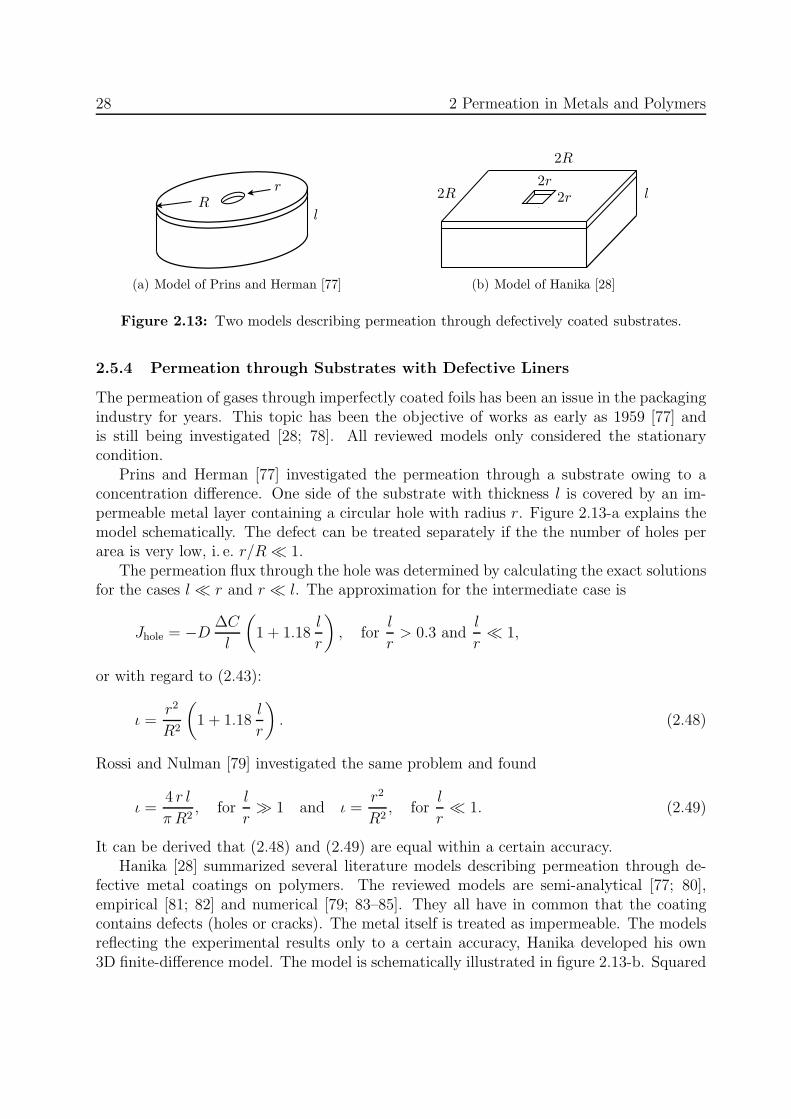
rR
(a) Model of Prins and Herman [77]
2r2r2R
2R
l
(b) Model of Hanika [28]
Figure 2.13: Two models describing permeation through defectively coated substrates.
2.5.4 Permeation through Substrates with Defective Liners
The permeation of gases through imperfectly coated foils has been an issue in the packagingindustry for years. This topic has been the objective of works as early as 1959 [77] andis still being investigated [28; 78]. All reviewed models only considered the stationarycondition.
Prins and Herman [77] investigated the permeation through a substrate owing to aconcentration difference. One side of the substrate with thickness l is covered by an im-permeable metal layer containing a circular hole with radius r. Figure 2.13-a explains themodel schematically. The defect can be treated separately if the the number of holes perarea is very low, i. e. r/R� 1.
The permeation flux through the hole was determined by calculating the exact solutionsfor the cases l � r and r � l. The approximation for the intermediate case is
Jhole = −D ∆C
l
(
1 + 1.18l
r
)
, forl
r> 0.3 and
l
r� 1,
or with regard to (2.43):
ι =r2
R2
(
1 + 1.18l
r
)
. (2.48)
Rossi and Nulman [79] investigated the same problem and found
ι =4 r l
π R2, for
l
r� 1 and ι =
r2
R2, for
l
r� 1. (2.49)
It can be derived that (2.48) and (2.49) are equal within a certain accuracy.Hanika [28] summarized several literature models describing permeation through de-
fective metal coatings on polymers. The reviewed models are semi-analytical [77; 80],empirical [81; 82] and numerical [79; 83–85]. They all have in common that the coatingcontains defects (holes or cracks). The metal itself is treated as impermeable. The modelsreflecting the experimental results only to a certain accuracy, Hanika developed his own3D finite-difference model. The model is schematically illustrated in figure 2.13-b. Squared

2.5 Permeation 29
Table 2.2: Comparison of the models to simulate permeation through defectively coated sub-strates.
study r R l r/R l/r ι (2.48) ι (2.49) ι (2.50)1 1 nm 10 nm 1.8mm 1 · 10−1 1.8 · 106 2.1 · 104 2.3 · 104 1.0 · 102
2 1 nm 100 nm 1.8mm 1 · 10−2 1.8 · 106 2.1 · 102 2.3 · 102 7.8 · 101
3 1 nm 1µm 1.8mm 1 · 10−3 1.8 · 106 2.1 · 100 2.3 · 100 3.4 · 100
4 1 nm 10µm 1.8mm 1 · 10−4 1.8 · 106 2.1 · 10-2 2.3 · 10-2 3.5 · 10-2
5 1µm 10µm 1.8mm 1 · 10−1 1.8 · 103 2.1 · 101 2.3 · 101 2.6 · 101
6 1µm 50µm 1.8mm 2 · 10−2 1.8 · 103 8.5 · 10-1 9.2 · 10-1 1.4 · 100
7 40µm 100µm 1.8mm 4 · 10−2 4.5 · 101 8.7 · 10-2 9.2 · 10-2 1.4 · 10-1
8 40µm 1mm 1.8mm 4 · 10−3 4.5 · 101 8.7 · 10-4 9.2 · 10-4 1.4 · 10-3
1 2 3 4 5 6 7 810-3
10-2
10-1
100
101
102
103
104 Prins&Herman Rossi&Nulman Hanika
ι
study
Figure 2.14: Comparison of the mod-els to simulate permeation through defec-tively coated substrates. The barrier con-stant is plotted versus the study parame-ters listed in table 2.2.
coating defects of width 2 r are separated by the characteristic defect distance 2R. Theadvantage of this model is that interactions of holes are taken into account. The barrierconstant is
ι =(r/R)2
1 − exp (−0.507 r/l) + 0.01 (r/R)2. (2.50)
The three presented models are compared by calculating the barrier constants of eightgeometry constellations. The study parameters and the results are listed in table 2.2. Thechosen parameters are representative for expected defects (study 1 – 4: “empty“ grainboundary, 5 – 6: microcracks, 7 – 8: holes). The results of the three models are similar aspresented in figure 2.14. The model of Hanika deviates from the two others only for greatratios between the substrate thickness and the defect distance. This behavior is attributedto the influence of neighboring holes which is taken into account only in his model.

30 2 Permeation in Metals and Polymers
1 2 3 4 5 6 7 8
1x10-19
1x10-18
1x10-17 He permeation H
2 permeation
sample
P /
mol
/m s P
a
Figure 2.15: Comparison of helium andhydrogen permeabilities of CFRP from [86].Each sample was tested at room temperaturewith hydrogen and helium. Although thepermeabilities vary strongly, in most casesthe helium permeability is greater than thehydrogen permeability.
2.5.5 Comparison of Hydrogen and Helium Permeation
The measurement of hydrogen permeation is often substituted by helium or argon as testgas for reasons of convenience [86–88]. This section gives a comparison of the H2 and Hepermeation in polymers and metals.
Considering polymers, the permeability, being a product of D and S (2.33), is mainlydependent on the gas size [41; 46]. While the diffusivity decreases with the penetrant’ssize, the solubility generally increases with the gas size [41]. Humpenoder [88] reports anexponential dependency of the gas radius on the diffusivity:
Dgas 1/Dgas 2 = exp(rgas 2/rgas 1).
Regarding size and mass, helium is the most similar gas to molecular hydrogen. The van-der-Waals molecular diameter of hydrogen and helium are 276 pm and 266 pm, respectively[89]. With the assumption of Humpenoder above, the diffusivities of hydrogen and heliumshould have a ratio of DHe/DH2
= 2.8. Humpenoder found in experiments with HDPE,PVC, PC and PA that the He diffusivity is 1.6 – 6.6 times greater then that of H2.
Measured helium permeabilities in polymers are reported to be comparable to or slightlygreater than those of hydrogen. Humpenoder [88], though the diffusivities varied, foundsimilar permeabilities in the considered materials. Goetz et al. [86] investigated the perme-ation through eight CFRP (IM7/977-2) samples. The results are presented in figure 2.15.Averaging the data, helium permeates slightly stronger than hydrogen. The transportproperties of ECTFE, LDPE, PP and PVC are reported in [48; 89–95]. The differences be-tween He and H2 are minor, though He exhibits a slightly greater permeability. O’Hanlon[96] reviewed the permeabilities of six polymeric materials. He concluded that the heliumpermeability is greater or equal the hydrogen permeability.
Considering diffusion through metals, hydrogen and helium exhibit different mecha-nisms, see 2.4.2. Few researches were carried out on the direct comparison of He and H2

2.6 Simulation of Permeation 31
permeation in metals. Schefer et al. [38] stated qualitatively that the helium diffusivity isseveral orders of magnitude lower than that of hydrogen. McCool and Lin [97] reported aH2/He selectivity at 573K for Pd-Ag membranes in the range of 23 to 4770. Collins andTurnbull [98] investigated the permeation of helium and hydrogen through 0.25mm thicktubes at 1023K. Hydrogen permeation was detected through Monel, 304 stainless steel,Kovar, Inconel, nickel, and 52 Alloy (Fe50Ni50) even at temperatures approaching roomtemperature. The same metals were not permeated by helium at temperatures as high as1123K.
Experiments to directly compare He and H2 permeation in grain boundaries have notbeen performed. However, it can be assumed that the permeation behavior of He and H2 ingrain boundaries is similar, when considering that primarily a vacancy motion is present,refer to 2.4.4.
Summarizing, helium and hydrogen exhibit comparable diffusivities and permeabilitiesin plastics and presumably in metals with grain boundaries. In metals, the permeabilityof hydrogen is much greater than that of helium.
2.6 Simulation of Permeation
The Fick curve (2.27) describes one-dimensional transient diffusion or permeation, re-spectively, in homogeneous membranes. However, this equation may not be employed inmulti-layer permeation, grain boundary diffusion or permeation through substrates withdefective liners. Hence, presuming inhomogeneous materials in general, the measured flux-time curves can differ from the Fick curve.
The reviewed simulations of grain boundary diffusion in 2.4.4 and permeation throughdefectively coated membranes in 2.5.4 only cover the stationary state. The only transientconsideration — of Hwang and Baluffi — may only be used in Harrison type C grainboundary diffusion.
In order to understand the reason for diversely measured J(t) curves in this workthough, own transient simulations are carried out. The developed model covers the diffusionin two dimensions. Considering the sorption equation (2.16), this model also allows tosimulate two-dimensional permeation. Various materials with different transport properties(D and S) and arbitrary geometries can be defined. Additionally, this model can take thedissociation of molecules into account. The physical assumptions underlying the used modeland their mathematical implementation into a program are described in the following.
Definition of the Diffusion Problem
The diffusion problem in one material is described by the two laws of Fick. Considering abody of different materials, Fick’s laws may only be applied to each material separately.Knowing the interface conditions, the overall system is determined and can be solved. Inthe following, the term phase is used for a continuous region of one material.

32 2 Permeation in Metals and Polymers
mij
mx,inij
dxj
dy i
my,outij
my,inij
mx,outij
(a) mass of the element and mass fluxes throughthe boundaries
ˆ
Cij
Jx,inij
dxj
dy i
Jy,outij
Jy,inij
Jx,outij
(b) concentration of the element and fluxesthrough the boundaries
Figure 2.16: Mass conservation of element (i,j)
Numerical methods are always based on the principle of discretizing the continuousmedia (into elements) and the time (into time steps). The simplest discretization principleis the finite difference method (FDM), which requires initial and boundary conditions.
In this thesis, the body is discretized into rectangular elements. The number of elementsin vertical and horizontal direction are denoted by v and w, respectively. Introducing amathematical index, these elements can be assigned. The element in the ith row and jthcolumn is indexed (i, j). Each element (i, j) is defined by its properties: width dxj , heightdyi, concentration in the center Cij, solubility Sij , diffusivity Dij , and pressure exponentnij (2.16). Discretizing the time into the increment ∆t, the explicit solution of the FDM is
Cij(t+ ∆t) = Cij(t) + Cij(t) ∆t. (2.51)
The unknown derivative of the concentration w. r. t. time can be determined by reformu-lating Fick’s second law (2.20).
Reformulation of Fick’s Second Law
Considering an element (i, j) as shown in figure 2.16-a, the increase of the mass inside theelement equals the sum of all mass flows into and out of the element boundaries
mij =∑
m|bound
= mx,inij − mx,out
ij + my,inij − my,out
ij .
The mass increase and the mass fluxes can be replaced by adequate expressions of theconcentration increase and the fluxes, respectively (refer to figure 2.16-b).
mij = M Cij dxj dyi dz
mx,in|outij = M J
x,in|outij dyi dz
my,in|out
ij = M Jy,in|out
ij dxj dz.

2.6 Simulation of Permeation 33
phase Φ1 phase Φ2
µ(x)
x∗ x
C(x)
(a) distribution of chemical potential and con-centration
phase Φ1 phase Φ2
x∗ x
C(x)Cij
linear approximation
(b) true concentration C(x), concrete values Cij
at the center of an element, and linear approxi-mation
Figure 2.17: Concentration distribution at an interface of two phases.
where M is the molar mass of the permeating gas. Substituting the equations above intothe equation of the mass balance one obtains
Cij =Jx,in
ij − Jx,outij
dxj+Jy,in
ij − Jy,outij
dyi. (2.52)
Equation (2.52) is another expression of Fick’s second law. It states that the sum of thenegative flux gradients is equal the concentration increase. The unknown fluxes throughthe element boundaries in (2.52) are determined in the following.
Fluxes through Element Boundaries
Figure 2.17 shows the general concentration distribution at the interface between twophases. The chemical potential, µ, is per definition continuous. The concentration ex-hibits a step if the solubilities of both phases are different. Although the flux inside aphase is determined by Fick’s first law (2.19), it may not be employed at the interface.
Figure 2.18 illustrates two adjacent elements, 1 and 2, of different phases Φ1 and Φ2.The relationship between the concentrations at the interface is derived by considering that
C1 C2J2
dx1 dx2
dy
C∗2C∗
1
J1
D1, S1, Φ1 D2, S2, Φ2
Figure 2.18: Concentrations and fluxes in two adjacent elements, 1 and 2.

34 2 Permeation in Metals and Polymers
the chemical potential of the dissolved gas (2.18) is equal in both elements at the interface
1
n1
µ1(x∗) =
1
n2
µ2(x∗) −→
(
C∗1
S1
)1/n1
=
(
C∗2
S2
)1/n2
, (2.53)
where n1 and n2 are the pressure exponents.Presuming no mass accumulation at the common boundary, the mass flows into and
out of the interface are equal, m1 = m2. The mass flow can be substituted by the flux:m = M N = M J A, where M is the molar mass and A is the interface area. The molarmass of the dissolved gas depends on the existence of dissociation, hence: M1/M2 = n1/n2.It follows for the boundary fluxes that
J1
J2
=n2
n1
. (2.54)
Presuming a linear distribution of the concentration from the center to the boundary ineach element (see figure 2.17-b), the fluxes are approximated by Fick’s first law
J1 = −D1
C∗1 − C1
dx1/2, (2.55)
J2 = −D2
C2 − C∗2
dx2/2. (2.56)
Rearranging (2.55) and (2.56) for C∗1 and C∗
2 , respectively, and substituting these expressionin (2.53) considering (2.54) one obtains
(
C1
S1
− n2
n1
J2
2D1 S1
dx1
)n2/n1
=C2
S2
+J2
2D2 S2
dx2. (2.57)
Defining the variable
γi =dxi
2Di Sifor i = 1, 2, (2.58)
the fluxes J1 and J2 are, depending on the ratio n2/n1,
n1
n2
= 1 : J1 = J2 = (γ1 + γ2)−1
(
C1
S1
− C2
S2
)
n1
n2
= 2 : 2J1 = J2 =1
4γ2
(
4C2
S2
+γ1
γ2
)
√
1 − 16
(
4C2
S2
+γ1
γ2
)−2 (
C22
S22
− C1
S1
)
− 1
n1
n2
=1
2: J1 = 2J2 =
−1
4γ1
(
4C1
S1
+γ2
γ1
)
√
1 − 16
(
4C1
S1
+γ2
γ1
)−2 (
C21
S21
− C2
S2
)
− 1

2.6 Simulation of Permeation 35
Cij
Jx,inij
Jy,outij
Jy,inij
Jx,outij
Ci−1j
dy i
−1
Jy,outi−1j
Ci+1j
dxj
dy i
+1
Jy,ini+1j
Cij−1
dy i
Jx,outij−1
dxj−1
Cij+1
Jx,inij+1
dxj+1
Figure 2.19: Element (i, j), its adjacent elements, and the fluxes through their common bound-aries
The unknown fluxes J of (2.52), being graphically explained figure 2.19, can now bereplaced by given concentrations.
Jx, in
out
ij =
nij∓1
nij=1 :
(
γxij∓1 + γx
ij
)−1(
∓Cij
Sij± Cij∓1
Sij∓1
)
nij∓1
nij=2 : ±1
4γxij
(
4Cij
Sij+
γxij∓1
γxij
)
[
√
1-16(
4Cij
Sij+
γxij∓1
γxij
)−2 (
C2ij
S2ij
− Cij∓1
Sij∓1
)
− 1
]
nij∓1
nij=1
2: ∓1
8γxij∓1
(
4Cij∓1
Sij∓1+
γxij
γxij∓1
)
[
√
1-16(
4Cij∓1
Sij∓1+
γxij
γxij∓1
)−2 (
C2ij∓1
S2ij∓1
-Cij
Sij
)
-1
]
(2.59)
Jy, in
out
ij =
ni∓1j
nij=1 :
(
γyi∓1j + γy
ij
)−1(
∓Cij
Sij± Ci∓1j
Si∓1j
)
ni∓1j
nij=2 : ±1
4γy
ij
(
4Cij
Sij+
γy
i∓1j
γy
ij
)
[
√
1-16(
4Cij
Sij+
γy
i∓1j
γy
ij
)−2 (
C2ij
S2ij
− Ci∓1j
Si∓1j
)
− 1
]
ni∓1j
nij=1
2: ∓1
8γyi∓1j
(
4Ci∓1j
Si∓1j+
γy
ij
γyi∓1j
)
[
√
1-16(
4Ci∓1j
Si∓1j+
γy
ij
γyi∓1j
)−2 (
C2ij∓1
S2i∓1j
-Cij
Sij
)
-1
]
(2.60)

36 2 Permeation in Metals and Polymers
where
γxij =
dxj
2Dij Sij; γy
ij =dyi
2Dij Sij. (2.61)
Implementation in a Program
In the most general case, the body to be simulated consists of different materials, i. e. differ-ent phases. It is mandatory to apply equations (2.52), (2.59) and (2.60) for each element.In detail, the following solution steps are run:
1. Set-up (discretization, definition of initial and boundary conditions)
(a) Definition of the grid dimension: i = 1..v and j = 1..w, where v and w are thenumbers of elements in vertical and horizontal direction, respectively.
(b) Definition of the grid shape: dxj and dyi, ∀ i, j(c) Definition of the material properties of each element: nij , Dij , Sij and φij, ∀ i, j(d) Definition of the initial concentration of each element: Cij(t=0) = C0
ij , ∀ i, j(e) Definition of the boundary elements (i, j) ∈ B, where B is the set of boundary
indexes. Boundary elements must be defined at least at the extends of thematrix. The boundary elements must not vary with time.
(f) Definition of the boundary conditions for each boundary element. Type 1:Dirichlet boundary condition Cij(t>0) = CB
ij or type 2: Neumann boundary
condition Jx/y,in/out
ij = 0, for (i, j) ∈ B. The boundary conditions may vary withtime.
(g) Definition of the time increment ∆t. In advanced programming the time incre-ment can depend on the progress of the simulation.
(h) Setting of time variable to zero: t = 0.
2. Solving
(a) Increase of time: tnew = t+ ∆t
(b) Calculation of the fluxes Jx,inij , Jx,out
ij , Jy,inij , Jy,out
ij according to (2.59) and (2.60)for all non-boundary elements (i, j) /∈ B.
(c) Calculation of the mandatory fluxes in the boundary elements (i, j) ∈ B. Ingeneral, one or more fluxes of (2.59) and (2.60) are zero.
(d) Calculation of the concentration increase Cij ∀ (i, j) according to (2.52).
(e) Calculation of the concentration at time tnew according to (2.51):Cnew
ij = Cij + Cij ∆t for all (i, j)

2.6 Simulation of Permeation 37
(f) Reallocation of the concentration and time variable:Cij = Cnew
ij , t = tnew
(g) Loop to step 2 (a) until simulation is finished
3. Post-processing
(a) Plotting of concentration distribution versus time
(b) Plotting of flux versus time
(c) Export of the data
Special Case: Different Phases without Dissociation
The solving method presented above requires a high computing effort. The equations(2.59) and (2.60) are calculated ni × nj times at every time step. Furthermore, theseequations are case-sensitive, which requires an “if-then” programming. The computingdurance with a personal computer is too high for extensive simulations being efficient. Inmany cases, different phases exist which have different diffusivities and solubilities, but thesame pressure exponent, n. For these cases, a method with increased efficiency is presented.
By considering nij = n ∀ (i, j). Equations (2.59) and (2.60) become simple:
Jx,in|out
ij =(
γxij∓1 + γx
ij
)−1
(
∓Cij
Sij
± Cij∓1
Sij∓1
)
Jy,in|outij =
(
γyi∓1j + γy
ij
)−1
(
∓Cij
Sij± Ci∓1j
Si∓1j
)
.
Inserting these expressions for the fluxes into (2.52), the concentration increase is
Cij =1
dxj
(
γxij + γx
ij−1
)−1
[
Cij−1
Sij−1
− Cij
Sij
]
+1
dxj
(
γxij + γx
ij+1
)−1
[
Cij+1
Sij+1
− Cij
Sij
]
(2.62)
+1
dyi
(
γyij + γy
i−1j
)−1
[
Ci−1j
Si−1j
− Cij
Sij
]
+1
dyi
(
γxij + γx
i+1j
)−1
[
Ci+1j
Si+1j
− Cij
Sij
]
.
Equation (2.62) contains only constant material properties, constant geometry variables,and the variable concentrations of the elements. Furthermore, the unknown concentrationincrease Cij is linearly dependent on the input variables, Cij. Hence, this equation can betransformed to a linear matrix equation C = f(T,C), where C is the concentration matrixand T is a constant coefficient matrix. In particular, the usage of linear algebra enablesenhanced and fast simulations. The results of the performed simulations are presented in6.3.

38 2 Permeation in Metals and Polymers

Chapter 3
Preselection of Feasible Liner Materials andProduction Processes
In order to narrow the wide range of liner materials, a preselection is done on basis ofpermeation and outgassing rates found in the literature. First of all, this chapter surveysexisting or planned liners of LH2 tanks. H2 permeabilities of metals, polymers and glassesreported in the literature are reviewed and compared in the following. Afterwards, theoutgassing process is briefly introduced and typical outgassing rates of several materialsare presented. After performing sample calculations to assess the required liner propertiesto enable a stable tank vacuum, potential liner materials are preselected. Finally, linerproduction processes are reviewed and evaluated.
3.1 Literature Review of LH2 Tank Liners
Mainly the space and aircraft industry has performed studies, tests and prototyping ofCFRP tanks. These tank systems can be categorized into four classes regarding their insu-lation technique. First amongst these are cryogenic tanks with one CFRP shell but neitherinsulation nor liner, produced by Wilson Composites [99] and Microcosm [100]. Both tanksystems are primarily conceived for liquid oxygen. Secondly, NASA and McDonnell Dou-glas have produced a LH2 tank consisting of one CFRP shell and an outside foam insulationbut containing no liner [101; 102]. Thirdly, sandwich solutions were employed in severaltank systems. The sandwich is made of CFRP skins and an insulating foam core. Three ofthese tank systems were produced or planned without liners [86; 99; 103; 104]. Three othertank systems by ESA [105–108], Northrop Grumman [99; 109] and NASA [87] considerthe usage of liners. Finally, vacuum insulated storage systems were produced or studied.ILK Dresden [110] produced LHe cryostats made of glass fiber reinforced plastics withoutliners for the measurement of low magnetic fields [111]. However, the vacuum stability waslimited to 1 – 2 months. Hartwig [112] studied fiber reinforced materials and liners forthe operation in LH2 tanks. In the following, the liners employed or investigated by ESA,NASA, Northrop Grumman and Hartwig are presented in more detail.
ESA. Since 1994, the European Space Agency has worked on reusable launch vehicles.Within the project FESTIP, two different tank concepts were developed but not produced.The first tank concept implied an aluminum-lithium waffle structure, a foam insulation anda liner facing the hydrogen [105]. The liner was planned to be a 0.1mm thin aluminumfoil. The second tank concept consisted of a CFRP sandwich solution with a liner [106].Five liner types were studied.
39

40 3 Preselection of Feasible Liner Materials and Production Processes
Three liner types facing the hydrogen were investigated by Diaz et al. [107]. The firstamong these types was a metal foil made of stainless steel or aluminum. The single foilsegments were joined by laser welding. The second liner consisted of collapsible metallicfoils or organic films. The ends of the liner were secured by retainer rings at the access ports.The third liner type was made of PBO and produced by an extrusion blow-molding process.Although tests revealed low permeation rates, the inherent manufacturing difficulties couldnot be solved.
Two alternative liners were studied by Antonenko et al. [108]. Firstly, metalized plasticfilms were proposed. The metallization, made of silver, gold or aluminum, should be appliedon organic base materials like PI, PTFE, PVC or PETP. Secondly, water dispersion coatingsbased on PU, VdC or PE were investigated. Thermal cycles between LN2 temperature and333K did not result in cracks or peeling-off. For both alternative liners, no information isgiven about liner thickness or permeation behavior.
Trading off all liner concepts, ESA selected foils made of 0.1mm thick aluminum(AA6061-TO). The trade off was carried out without any permeation tests on that liner.
NASA. In NASA’s X-33 program, a planned successor of the Space Shuttle shouldhave been developed. The employed LH2 tank consisted of a sandwich, made of CFRP facesheets and an insulating core, but no liners. The tank was destroyed in 1999 during testing.The subsequent investigation determined the most probable failure cause. Microcracksappeared in the inner facesheet and cold, gaseous hydrogen gas could infiltrate the core.The reduced bondline strength and high pressure inside the core led to the delaminationof the outer facesheet [86].
The X-33 program was canceled in 2001 [113]. The investigations and improvements,however, have been continued by Grimsley et al. [87]. Their work concentrated on theapplication of polymer film liners in and on the CFRP substrate. The permeation testswere performed using Argon instead of hydrogen.
Aluminized Mylar films provided the highest potential considering the permeation.The 0.023mm or 0.1mm thick Mylar films were coated with 300 A aluminum by means ofphysical vapor deposition. Although the potential of reducing the permeability was shown,a high scatter of the results was also reported. The scatter was attributed to variations inthe process conditions. Mechanical tests performed on CFRP with an interleaf aluminizedMylar film resulted in delamination.
Northrop Grumman Corporation developed a cryogenic fuel tank made from com-posite materials for NASA’s Marshall Space Flight Center [114], see figure 3.1. The tankwas made of a composite sandwich structure with a liner. The liner consisted of a thinaluminum foil enclosed by epoxy resin films [99]. The epoxy-aluminum-epoxy film was ap-plied between the consolidated inner skin and the honeycomb core. Starting in November2003, tests were performed for the next 9 months. Joan Funk, NASA’s cryogenic tanksproject leader, reported: “We didn’t prove that composite fuel tanks don’t leak! In fact wehave a hydrogen leak we just don’t know if its from the tank or the plumbing.” [115]
Hartwig [112] investigated fiber reinforced materials enhanced with different liners. Allinvestigated surface liners (12µm sputtered TiN, 2µm sputtered amorphous carbon, 0.5µmchemical NiP and 10µm chemical/electrochemical Cu) did not reduce the permeation rate.

3.2 Literature Review of Hydrogen Permeabilities 41
Figure 3.1: Composite liquid hydrogen tank man-ufactured by Northrop Grumman. From [109].
Embedded foil liners made of Al (240 µm) and Sn (100 – 200µm) were not permeatedby helium and hydrogen. Because the aluminum foil separated from the CFRP, Hartwigrecommended a thin tin foil as a liner.
Summarizing, the few liners used or planned for composite LH2 tanks can be categorizedinto foils or coatings. Metallic foil liners were proposed by ESA, Northrop Grumman andHartwig. The investigated foils were made of aluminum, stainless steel and tin. Metalizedplastic films were investigated by ESA and NASA. The coating materials were aluminum,silver and gold. None of these liners were applied on a vacuum-insulated LH2 tank madeof CFRP.
3.2 Literature Review of Hydrogen Permeabilities
This section reviews the H2 permeabilities and, if available, the related activation energiesfound in the literature. A distinction between metals, polymers and glasses is made. Thereviewed data are listed in table A.1 – table A.9 of appendix A and partly plotted infigure A.1 – figure A.5. For a wide range of diffusivities in metals, it is referred to thepublications of Wipf [51] and Volkl & Alefeld [116].
The literature review leads to the following statements: 1. For some materials, only veryfew or even only one measurement is existing. 2. In few cases, the measured permeabilitiesof one metal vary more than five orders of magnitude. 3. The permeabilities of metals ismostly determined at high temperatures. The extrapolation to room temperature (RT)must be considered carefully. 4. A direct relationship between the structure of the metallattice (refer to 2.1) and the measured permeabilities does not exist.
The permeabilities of metals on one hand and those of polymers or glasses on theother hand are defined differently, depending on the existence of dissociation (see 2.5.1).The dimension of P in metals and polymers is mol/m sPa0.5 and mol/m sPa, respectively.Consequently, the permeabilities cannot be compared directly. Instead, the permeationfluxes owing to a defined pressure difference are evaluated. Considering feed pressuresbetween 1 bar and 6 bar, equal permeation fluxes through metals and polymers exist, if|Pmetal| ≈ 500 |Ppolymer|.
Regarding their room temperature permeabilities, metals and alloys are here classified

42 3 Preselection of Feasible Liner Materials and Production Processes
10-29
1x10-24
1x10-19
1x10-14
1x10⁻⁹
elas
tom
er
ther
mos
et
ther
mop
last
glas
s
SS
Fe
allo
y
Fe
Ni a
lloy
Ni
Cu
Au
Al
P /
mol
/m s P
a0.5
material
10-27
10-22
10-17
1x10-1210-12
P /
mol
/m s P
a
Figure 3.2: Comparison of room temperature H2 permeabilities in some metals, polymers andglasses. The scales for metals and polymers are arranged so that the resulting permeation fluxesfor pf = 1 . . . 5 bar are approximately equal. The plotted data are from appendix A.
into 3 categories: extra-low permeation materials (|P | < 10−20), low permeation materials(10−20 < |P | < 10−17) and high permeation materials (|P | > 10−17). Extra-low permeabil-ities are found in germanium, tungsten, gold, aluminum and silver. Platinum and coppercan be classified between extra-low and low permeation materials. Low permeation ma-terials are cobalt, beryllium and nickel. Stainless steel, iron and nickel alloys can be highor low permeation materials, depending on their composition. Iron and titanium are highpermeation materials with P ≈ 10−13 mol/m sPa0.5. Very high permeabilities can be foundin palladium, vanadium, tantalum and yttrium.
The RT permeabilities of glasses are between 10−16 and 10−24 mol/m sPa. The polymerpermeabilities are all within a bandwidth of three orders of magnitude, if six highly per-meable materials are neglected. P (RT) ranges between 10−17 and 10−14, while the averageis approximately at 10−15 mol/m sPa. The RT permeabilities of glasses and polymers aregraphically compared with those of some metals in figure 3.2. The lowest permeabilities canbe found in some metals followed by glasses. The permeabilities of polymers are relativelyhigh.
The permeabilities of all polymers and all low or extra-low permeation metals extrap-olated to T = 20K are negligible. The permeabilities are less than 10−53 mol/m sPa or10−62 mol/m sPa0.5, respectively. The extrapolated permeability of gold at 20K is even10−306 mol/m sPa0.5.
3.3 Outgassing and Literature Review of Outgassing Rates
Outgassing is the gas release from a solid’s surface. It can be classified into two differentprocesses. Firstly, molecules dissolved in the bulk diffuse to the surface and desorb from it.This process is denoted thermal outgassing [117]. Secondly, particles that have previouslybeen adsorbed, e. g. at high pressures during venting a vacuum chamber, desorb from thesurface again. This process is called short-time outgassing [118]. In general, both processesare existing concurrently. The predominant outgassing molecule in polymers is water vapor

3.3 Outgassing and Literature Review of Outgassing Rates 43
Table 3.1: Area specific outgassing rates in mbar l/s m2 of stainless steel as a function of bake-outtime and bake-out temperature T . The data are taken from [128].
bake-out timeT / °C 20h 40 h 100 h 200 h
150 9.0 · 10−07 7.6 · 10−07 4.0 · 10−07 2.9 · 10−07
250 9.0 · 10−08 7.6 · 10−08 4.0 · 10−08 2.9 · 10−08
400 5.7 · 10−09 2.4 · 10−09 1.4 · 10−09 1.4 · 10−09
500 1.1 · 10−10 1.1 · 10−11 5.7 · 10−13 1.1 · 10−14
[119]. In metals, water vapor and mainly hydrogen are the sources of outgassing [120–122].Besides thermal and short-time outgassing, atoms or molecules are released from the
surface if the vapor saturation pressure is higher than the vacuum pressure. The vaporsaturation pressure of most metals is lower than 10−8 mbar at room temperature and muchless at 20K [70; 96]. Some polymers vaporize at high pressures, for instance Teflon at10−7 mbar and Perbunan at 5 · 10−4 mbar, respectively.
The outgassing rate is defined in two different ways. In space applications, the totalmass loss (TML) is used to characterize polymers [123; 124]:
TML =∆m
m∆t,
where m is the mass of the subjected material at the beginning and ∆m is the mass lossduring time ∆t. The test procedure is described in [125]. The investigated material withm ≈ 250mg is placed inside a copper chamber. This chamber is heated to 125 °C for24 hours. The released gas can escape only through a 6.3mm diameter exit port. Thedisadvantages of this method are the standard temperature of 125 °C, the non-existence ofvacuum, no relation to an area and the very low accuracy.
In most publications, the outgassing rate is defined as a gas flow or an area-specific gasflow
QG =d(p V )
dtor qG =
1
AQG. (3.1)
The outgassing rate depends on the temperature and on the time. At high tempera-tures, the outgassing is accelerated. Presuming thermal outgassing, Calder and Lewin [126]have analytically shown that the outgassing rate is proportional to exp(− 1
T). Kishiyama
et al. [127] state that below 373K, the outgassing rate doubles with each temperatureincrease of 15K. The bake-out process takes advantage of the strong temperature depen-dency. After heating and subsequent cooling, the outgassing rate is dramatically decreased.Table 3.1 shows the strong emphasis of the bake-out temperature in comparison to thebake-out time exemplarily for hydrogen outgassing from stainless steel.
Wutz, Adam and Walcher [30] distinguished between three functions of QG(t). Whilethe outgassing kinetics of metals are generally described by QG ∝ t−1, polymers can follow

44 3 Preselection of Feasible Liner Materials and Production Processes
10-12
1x10⁻¹⁰
1x10⁻⁸
1x10⁻⁶
1x10⁻⁴
1x10⁻²
1x100
polymersceramicsglasses
Ti, TiNCuAlSS
q G
/ m
bar
l/s m
2
Figure 3.3: Area specific outgassing rates at RT of stainless steel, aluminum, copper, titanium,ceramics, glasses and polymers from literature. The plotted data are from appendix B.
either QG ∝ t−1/2 or QG ∝ exp(−t). Dylla et al. [129] measured the outgassing rates ofstainless steel and aluminum and found that QG ∝ t−n with n = 0.9 . . . 1.3.
The outgassing rates of various materials are reviewed from the literature and listed inappendix B. Figure 3.3 compares the outgassing rate of stainless steel, aluminum, copper,titanium, ceramics/glasses and various polymers. The minimum area specific outgassingrate of various polymers is 5 · 10−7 mbar l/sm2 at room temperature. The minimum valuesof metals are much less. Outgassing rates of approximately 10−11 mbar l/sm2 are reportedfor stainless steel and copper.
3.4 Vacuum Stability and Material Preselection
The parameters to mathematically describe the LH2 tank of chapter 1 are presented infigure 3.4. The approximate values of these parameters are Vv ≈ 0.06m3, Ai ≈ 1.6m2,pH2
≈ 6 bar and Tv ≈ 293K. In a first assessment, the pressure of the vacuum insulationmay not exceed 5 · 10−4 mbar within 2 years. It follows that the maximum allowable totalgas flow into the insulation space is
Qmax =d(p V )
dt=
∆pv
∆tVv ≈ 5 · 10−4 mbar
2 a0.06 m3 = 5 · 10−10 mbar l/s. (3.2)
To assess the maximum allowable permeation and outgassing rate, it is assumed that
QP,max = QG,max = 0.5Qmax = 2.5 · 10−10 mbar l/s, or
qP,max = qG,max = 0.5Qmax/Ai = 1.5 · 10−10 mbar l/s m2.(3.3)
At low temperatures, no significant outgassing will occur. On the contrary, cryopump-ing can even improve the vacuum. However, it must be assumed that the inner tank can

3.4 Vacuum Stability and Material Preselection 45
Ai
Vv
lpH2
Tv, pv
Figure 3.4: Parameters to describe theLH2 tank. Ai, Vv and l denote the sur-face area of the inner tank, the volume ofthe vacuum and the thickness of the in-ner tank, respectively. pH2
and pv are thepressures of the stored hydrogen and thevacuum, respectively. Tv is the tempera-ture of the vacuum.
also reach room temperature, for instance during manufacturing, delivery or service times.The minimum area specific outgassing rates of metals and polymers from 3.3 are comparedto the requirement (3.3):
qG,min,metals = 1 · 10−11 mbar l/s m2 < qG,max
qG,min,polymers = 1.3 · 10−6 mbar l/s m2 � qG,max.
The high outgassing rate of polymers at room temperature would correspond to a vacuumstability time of only four minutes. Hence, regarding outgassing, it is mandatory to applya metallic liner on the CFRP.
The permeation gas flow strongly depends on the temperature. At high temperatures,e. g. at RT, the gas flow is maximal and hence critical. With (2.7) and (2.34), the steady-state H2 permeation rate through the inner tank is
qP = RTv P (T )pn
H2
l. (3.4)
Let qP < qP,max, the maximum allowable permeability is
P < 1.656 · 10−17 mol
m s Pa1/2
l
mfor metals, and
P < 2.138 · 10−20 mol
m s Pa
l
mfor polymers and glasses.
These equations relate the permeability of a material to the required thickness, or viceversa. The CFRP of the inner tank with l ≈ 2mm would require a permeability of4 · 10−23 mol/m sPa or less. This value is not feasible for polymers at room temperature,refer to 3.2. The minimum RT permeability found in the literature is 10−17 mol/m sPa,which results in a steady-state gas flow of 10−4 mbar l/s. This value corresponds to avacuum stability time of only 5 seconds.

46 3 Preselection of Feasible Liner Materials and Production Processes
Table 3.2: Required liner thicknesses lmin for several metals presuming a vacuum stability oftwo years at 293 K (RT). The permeabilities are taken from appendix A.
metal P (293K) / mol/m sPa0.5 lmin remarksAg 1.2 · 10−24 73 nm extrapolated from T � 293KAl 1.4 · 10−27 . . . 4.4 · 10−19 0.08 nm – 26mmAu 6.3 · 10−34 . . . 6.2 · 10−27 4 · 10-17 – 4 · 10-10 mCu 1.3 · 10−20 . . . 9.9 · 10−19 0.8 . . . 60mmGe 3.2 · 10−41 2 · 10−24 m extrapolated from T � 293KMo 9.3 · 10−22 . . . 2.1 · 10−17 56µm . . . 1mSS 1.3 · 10−19 . . . 2.5 · 10−15 8mm . . . 150mW 4.9 · 10−32 . . . 7.3 · 10−24 3 · 10−15 . . . 10−7 m extrapolated from T � 293K
Feasible permeation barriers are either glass or metals. The minimum permeability ofglasses from literature is 3 ·10−24 mol/m sPa (see table A.6). This would imply a minimumliner thickness of 140µm. Considering metals as liner, the required thicknesses are calcu-lated for potential low and extra-low permeation materials and are listed in table 3.2. Thethicknesses range from 10−24 m for Germanium to 150m for stainless steel.
Summarizing, the outgassing and permeation rates of polymers at room temperatureare too high to enable a long-time stable vacuum. Hence, fiber reinforced plastics can onlybe introduced as a structural material of a vacuum-insulated LH2 tank if a liner is added.The mandatory liner must be applied at least on the surface pointing to the vacuum, thatmeans on the outside of the inner tank. The material of the liner should be either a metalor glass. Considering the availability, producibility and existing applications in UHV, gold,aluminum, and copper are preselected. With regard to the literature survey of liners in3.1, tin will also be further investigated.
3.5 Literature Review and Preselection of Liner Production Pro-
cesses
Liners can be categorized into foils/sheets or coatings. Foils and sheets are manufacturedin advance and then adhered on the substrate. Coatings are generally produced directly onthe substrate. Figure 3.5 gives a graphical overview of existing liner production methodswhich are explained in the following.
Foils or sheets can be produce in different thicknesses by means of rolling or deepdrawing [131]. Rolling implies a dense structure of these liners. The foils can be adheredon or laminated into the CFRP. Another technique is the lamination of CFRP on foilsor sheets. The joining of separate foil segments is difficult. A feasible joining method iswelding but the produced heat and its impact on the CFRP must be considered. It isreasonable though, to adhere different foil segments on the CFRP and close the joininglines by a subsequent coating process.

3.5 Literature Review and Preselection of Liner Production Processes 47
metallic liner production
foils and sheets coatings
adhering laminating vapor
depositioncladding varnishing thermal
spraying
metal
plating
Figure 3.5: Technologies to produce metallic liners. Partial source: [130].
The two variants of vapor deposition are physical vapor deposition (PVD) and chem-ical vapor deposition (CVD). PVD is defined if vapor is created by evaporation or sputter-ing. If the vapor is produced by chemical reactions, the process is called CVD. The processtemperature of CVD is generally very high (>700 °C, [132]). In all vapor deposition tech-niques, the vapor is transported in vacuum to the target and precipitates there. Vapordeposition is characterized by low deposition rates and brittle coatings. Brittle coatings onsoft substrates like CFRP tend to the formation of microcracks (eggshell effect, [133–135]).
Cladding liners can be produced by welding, hot dip coating or roll-bonding [130]. Allcladding technologies are disadvantageous because of the high production temperatures(near melting temperature of the metal) or pressures. They are not suitable for coating ofpolymers.
Varnishes can be produced with metallic or organic particles. Metallic varnishes arebaked at temperatures higher than 350 °C to vaporize the solvent [130]. Consequently, theyare not suitable for the application on CFRP. Organic varnishes are characterized by highoutgassing rates and are not an appropriate liner, either.
Different variants of thermal spraying exist. Commonly employed technologies arethe atmospheric and low-pressure plasma spraying and cold spraying [136; 137]. All thermalspray techniques have in common that the metal is melted and then carried to the substrate.Further information about the process is given in [136]. Depending on the coating material,the process temperatures are very high. Song et al. [138] reports a generally existingporosity of the coating.
Metal plating is a coating process in which ions of the coating metal are dissolved inan electrolyte and, by supplying electrons, are discharged and deposited onto the surface ofthe target (refer to figure 3.6). Depending on the source of the electrons one distinguishes
targ
et
Mez+
Me
z·e-
Figure 3.6: Principle of metal plating: metal ions Mez+
are discharged and deposit on the target’s surface.

48 3 Preselection of Feasible Liner Materials and Production Processes
targ
et
Mez+
z·e-
R
Rz+
e-
e-
e-
e-
e-
(a) The reduction agent R oxidizes and deliverselectrons to the target’s surface
targ
et
Mez+
Me
(b) The metal ions Mez+ are discharged by theelectrons on the surface and form the coating.
Figure 3.7: Principle of electroless plating
between electroless plating (without outer voltage source, also known as chemical deposi-tion, electroless deposition) and electroplating (with outer voltage source, also known aselectrochemical deposition and electrodeposition). While the deposition rate of electro-less plating is rather low (≈ 1 . . . 3µm/h), the rates of electroplating can be much higher(≈ 12µm/h) [139]. Because fiber reinforced plastics are non-conducting, they must ini-tially be covered by an electroless coating and can subsequently be coated by means ofelectroplating. The process temperatures of metal plating can be as low as 25 °C. A fullcoverage of the CFRP is feasible. The two classes of metal plating are further explained inthe next paragraphs.
Industrial-relevant methods of electroless plating utilize reducing agents for the sup-ply of electrons. There are two processes describing the chemical deposition: the oxidationof the reducing agent and the discharge of the metal ions (refer to figure 3.7). The sum ofboth processes is [130]
R −→ Rz+ + z · e-
Mez+ + z · e- −→ MeR + Mez+ −→ Rz+ + Me
,
where R is the reducing agent and Mez+ is the z-valent metal.
Common electroless depositions on polymers are chemical copper (cCu) and chemicalnickel phosphor (cNiP). Exemplarily, the cNiP process is presented. The two main compo-nents of the electrolyte are the metallic salt, nickel sulfate (NiSO4) and the reducing agent,mostly sodium hypophosphite (NaH2PO2). The stability of the electrolyte can be affectedby many factors like local heating, too high concentration of the reducing agent or dirtparticles. Stabilizing agents, complexing agents, pH-regulators and accelerators are addedto the electrolyte, in order to maintain its stability and allow a controlled deposition pro-cess. The target’s surface is activated in advance by means of palladium atoms, which actas germ cells. Subsequent, small crystals of the metal adsorb on the surface, move to andprimarily deposit at these germs. Depending on the type of the growth, the different germsform a grain-like surface morphology. These grain-like structures are not monocrystallineand must be distinguished from the grains defined in the crystallography. The shape and

3.5 Literature Review and Preselection of Liner Production Processes 49
⊕
e- e-
targ
et
Me
cathode anodeM
e
+-
⊕
⊕
⊕
⊕
⊕
⊕
⊕
⊕
⊕
⊕⊕
⊕⊕
⊕ ⊕
⊕⊕
⊕
Figure 3.8: Principle of electroplating: metal ions Mez+
(denoted with ⊕ in the diagram) are discharged and depositon the target’s surface.
size of these grain-like structures depend on the current density, the electrolyte, the shapeand the material of the substrate. The typical size of these grains is several micrometers.
The cNiP deposition is a sum of several reactions. The simplified net equation is
3NaH2PO2 + 3H2O + NiSO4 −→ 3NaH2PO3 + H2SO2 + 2H2 + Ni.
The electroplating process consists of three subprocesses. In the first step, the coatingmaterial, Me, is provided by an anode (refer to figure 3.8). In contact with the electrolyteand under specific conditions, the metal can spontaneously leave the lattice of the anodeand form metal ions in the electrolyte. As a result, the anode becomes negative becauseof an oversupply of electrons. This process is called anodic metal dispersion:
Me � Mez+ + z · e-.
The equilibrium can be changed to the right-hand side if an external voltage source isapplied so that the electrons are extracted from the anode.
In the second step, the metal ions diffuse to the target driven by an electric field. Theelectric field is created by supplying the target (cathode) with electrons, see figure 3.8. Inthe last step, the metal ions discharge at the surface of the target and form the coating.Similar to electroless plating, the deposition starts at favored spots (germs) and formsgrain-like structures.
Preselection of Liner Production Processes
Considering the production of the liner, the following requirements and criteria must befulfilled:
• feasibility to produce a closed, metallic liner in general
• feasibility to produce a liner on large structures (at the outside of the inner tankshown in figure 1.5-a)
• feasibility to produce a liner on complex geometries (free-form geometry of the LH2
lightweight tank)
• low costs, outlay, complexity and application time.

50 3 Preselection of Feasible Liner Materials and Production Processes
Taking these qualitative specifications into account, the metal-plating process shows thehighest potential. Hence, the majority of the liners investigated in this work are producedby this process. Considering the statements from 3.1, foils and sheets are also tested. FewPVD and thermal spray coatings are also investigated.

Chapter 4
Materials
This chapter presents and characterizes the materials used in the permeation measure-ments. First, the CFRP substrates are introduced in 4.1. The following section 4.2 de-scribes the materials, application methods and properties of the used liners. Section 4.3explains the geometry and preparation of the specimens.
The materials are classified into material systems. A material system is representedby a code starting with “M” and followed by two numbers, e. g. M01. The specimens areanalogously indexed by the abbreviations S01, S02, . . . . Numbers ending with c denotespecimens used at cryogenic temperatures.
4.1 Substrates
Different CFRP substrates exist, because the polymeric material of the tank structure wasdeveloped and defined parallel to the liner application pretests. Hence, the liners wereproduced on two different substrates, denoted by M02 and M03. Further CFRP samples(M04) were not employed for the liner production but for comparing the permeability withthose of M02 and M03. PVC specimens (M01) were used for validating the permeationapparatus because of their well-known transport properties. An overview of the polymericmaterial systems and their properties is given in table C.1 on page 129. In the following,the material systems M02 and M03 are presented in more detail.
The substrates representing the chosen tank material (M02) were produced by companyC02. The composite (Sigratex KDK 8054/120 carbon fibers and Araldite LY 564 withhardener HY 2954 epoxy resin) consists of six plies of woven fabric. The epoxy resinwas infiltrated by means of the VARI (vacuum assisted resin infusion) technique. There,an aluminum tool is firstly painted by a release agent. The laid-up fiber plies are thencovered by a perforated foil, a resin distribution medium and the vacuum bag1. At onelocation of the vacuum bag, a low vacuum is generated. At the opposite side of thevacuum bag, the heated, viscous resin is introduced to the carbon fiber lay-up. Driven bythe pressure difference between atmosphere and vacuum, the resin infiltrates the lay-up.After infiltration, the material is cured to let the epoxy groups fully react. The thicknessof the M02 specimens is between 1.4 and 1.8mm. A cross section is shown in figure 4.1.
The substrates of M03 were produced by company C01. They are made of Zoltek HTcarbon fibers and Bakelite epoxy resin (EPR04695 with hardener EPH05357). In opposite
1The influence of the resin, fibers, mold release agent, peel-ply and distribution medium on the abilityto apply a liner on the substrate was investigated in extensive tests. Based on these investigations, theresin and the helpers were chosen.
51

52 4 Materials
200 µm
Figure 4.1: SEM image of the polished sec-tion of a CFRP sample (M02). The wovencarbon fibers can be recognized. Resin richareas (bright) exist between the plies and atthe surface (bottom of image).
50 µm
(a) surface
50 µm
(b) polished section
Figure 4.2: SEM images of a CFRP sample (M02) after thermal shock. Microcracks form anetwork on the surface. The polished section image shows that the microcracks tend to originatein resin rich areas.
to M02, the substrates of M03 were produced by means of RTM (resin transfer molding)and cured in an autoclave. The thickness of the samples is approximately 2.5mm.
Composites tend to the formation of microcracks during thermal shock owing to theirheterogeneity. The thermal expansion coefficient of epoxy resin at 20K and 300K is ap-proximately 4 · 10−6 K−1 and 90 · 10−6 K−1, respectively [112]. In comparison, the thermalexpansion coefficient of carbon fibers is near zero or even negative in fiber direction [112].Cooling from RT to 77K (condensation temperature of nitrogen), the difference of thethermal strain between epoxy resin and carbon fibers is more than 1%. Figure 4.2 depictsthe microcracks of M02 after a thermal shock in LN2. The cracks form a network on thesurface. No microcracks were found that traverse the whole CFRP plate. In various testsit was shown that the microcrack density became maximal after 3 – 15 thermal shocks.
The maximum application temperature of the used epoxy resins is between 128 °C and145 °C. Consequently, the temperature of the liner production and the bake-out process isrestricted to these values.

4.2 Liners 53
10 µm
(a) SEM of the surface of a stain-less steel sheet (M06)
50 µm
(b) SEM of the surface of an alu-minum foil (M08)
(c) welded aluminum sheet (M05)
Figure 4.3: SEM images and photos of sheets and foils.
4.2 Liners
This section introduces the liners studied in this work. Their basic properties like out-gassing, thermal shock resistance, adhesive strength, structure and potential material de-fects are discussed. First, the methods to determine these properties are briefly explained.
Although quantitative measurements of the outgassing rate were not performed, quali-tative statements can be given by evaluating the vacuum pressure during the permeationmeasurements. All samples containing a liner, independent from the liner material, re-vealed a reduced outgassing rate compared to CFRP by factor 10 – 100. The generalappearance and the structure of the liner was determined by means of SEM. There, thesurface as well as the section of the liner was inspected for grains, holes, uncoated spots,microcracks or other material defects. EDX scans were performed to determine the compo-sition of the liner if necessary. The thermal shock resistance was tested by immersing thesamples three times into liquid nitrogen. Before each immersion, the samples were kept atroom temperature. After the thermal shock, potential microcracks were detected by meansof SEM. A possible peeling of the liner was observed by eye or by inspecting polished-cutimages. Grid tests according to DIN EN ISO 2409 [140] were performed to determine theadhesive strength.
Foils and Sheets
The foil and sheet liners (see table C.2) were made of aluminum, stainless steel, tin andcopper. The thickness of the sheets was between 0.21mm and 1.0mm. The foils were 25– 130µm thick and either adhered on substrates or single. The surface of sheets and foilswas free from defects like holes or microcracks but contained scratches (see figure 4.3). Theadhesive strength of foils on the substrates was very low in some cases and resulted in atotal peeling-off. Three samples of an aluminum sheet (M05) were welded to investigate afeasible sheet joining process (see figure 4.3-c).

54 4 Materials
20 µm
(a) surface
50 µm
(b) surface: existence of cracks
20 µm
(c) section: existence of cracks
Figure 4.4: SEM images of the cNiP coating (M12)
5 µm
(a) surface
2 µm
(b) surface: close-up of one grain-like structure
5 µm
(c) section
Figure 4.5: SEM images of the cCu coating (M31).
Metal Platings
The various studied metal platings and their basic properties, like liner material and thick-ness, are summarized in table C.4. All liners consisted of a chemical deposition layer toestablish a conductive area. This starting layer was followed by one or more functionallayers. The functional layer(s) was (were) mostly produced by means of electroplating.The metal platings can be classified regarding their starting layer.
The starting layer of M12 – M17 was a chemical nickel layer phosphor (cNiP) withapproximately 4 – 10µm in thickness (see figure 4.4). This cNiP coating contained regular,circular, grain-like structures (figure 4.4-a), and microcracks (figure 4.4-b,c). The size ofthese grains was between 3 and 8µm. The microcracks, mainly located along the grainboundaries, became more developed after thermal shock. The cracks totally traversed thecoating and extended into the resin. The existence of microcracks before the thermal shockpoints to a brittle behavior of the chemical nickel.
The initial layer of the material systems M18 – M26 was made of chemical copper (cCu,see figure 4.5). The cCu coating with circa 2µm in thickness was strongly textured. Thegrain-like features were regular, nearly circular and between 1 and 3µm in diameter. Inopposite to cNiP, cCu did not contain microcracks.

4.2 Liners 55
500 µm
(a) surface
100 µm
(b) section
10 µm
(c) section: void and channels
Figure 4.6: SEM images of the cNiP-Al coating (M13, S64)
50 µm
(a) surface
5 µm
(b) section
5 µm
(c) section: discontinuous Aulayer
Figure 4.7: SEM images of the cNiP-cAu coating (M14)
The functional coatings following the cNiP layer were made of aluminum, chemicalgold (cAu), copper, tin or nickel sulfamate (Ni)2. Aluminum coatings were produced fromaprotic electrolytes [141; 142]. The thickness of the gold layer was 0.3µm, those of theother functional layers were between 20 and 88µm.
The surfaces of M13 – M15 contained regular, circular, grain-like structures, refer tofigures 4.6-a, 4.7-a and 4.8-a. The size of these grains was between 3 and 8µm for cNiP+cAu(M14), between 25 and 55µm for cNiP+Cu (M15) and between 80 and 160µm for cNiP-Al(M13). Considering the cNiP-cAu and cNiP-Cu coatings, the cross sections showed thatthe heights of these grain-like features were small compared to the diameter (figures 4.7-b and 4.8-b). The height of the grain-like structures of the cNiP-Al liner was maximal20µm (figures 4.6-b) and hence considerable. The cNiP-Ni coating contained irregular,nearly crystalline, grain-like features, refer to figure 4.10. The size of these grains variedfrom less than 100 nm to 3µm. The cNiP-Sn coatings (M16, figure 4.9) did not contain arecognizable surface texture but regularly formed dents.
Besides grain-like structures, microcracks were observed in the Sn coatings (M16) after
2Nickel sulfamate coatings contain 100 % nickel. The term is derived from the electrolyte,Ni(SO3NH2)×H2O. This Ni coating was additionally proposed by the producer.

56 4 Materials
200 µm
(a) surface
50 µm
(b) surface: close-up
100 µm
(c) section
Figure 4.8: SEM images of the cNiP-Cu coating (M15)
500 µm
(a) surface
500 µm
(b) section
100 µm
(c) section: after thermal shock
Figure 4.9: SEM images of the cNiP-Sn coating (M16). Dents are existing in the coating (figurea and b). Microcracks appeared during thermal shock.
thermal shocks (figure 4.9-c). This behavior can be explained by the phase transition of tin.When tin is cooled below 13.2 °C, it changes from β-tin (7.29 g/cm3) to α-tin (5.77 g/cm3)[143; 144]. In the remaining coatings, no microcracks were observed before or after thermalshocks.
The cross sections of the coatings revealed two features. First, the Al coating wasinterspersed by channels (figure 4.6-b,c). Another specimen (S07) was not fully coveredby the aluminum layer. Second, the Au coatings were partly not fully deposited (seefigure 4.7-c). The remaining coatings showed a homogeneous thickness and a full coverage.
The adhesive strengths of the coatings were variable. The adhesive strength of thecNiP layer on CFRP was approximately 21MPa [145]. In contrast to this high value, thecNiP-Ni coating of M17 peeled off from the substrate during sawing. The grid tests of theremaining coatings revealed a sufficient high adhesive strength.
The functional coatings following the cCu layer were made of Cu (M18 – M22), Cu-Ni-Au (M23), Ni (M24), Ni-Au (M25) and Sn (M26), refer to table C.4. While the coatings ofM18 were deposited using standard process parameters, those of M19 – M22 were producedby a varied current density and sulfuric acid (H2SO4) concentration of the electrolyte, seetable C.4. Thereby, the influence of the parameters on the coating was investigated.

4.2 Liners 57
10 µm
(a) surface
50 µm
(b) section
Figure 4.10: SEM images of the cNiP-Ni coating (M17).
100 µm
(a) surface: no texture visible
100 µm
(b) section
Figure 4.11: SEM images of the cCu-Cu coating (M18, S42).
The surfaces of the cCu-Cu coating of M18 did not contain a recognizable texturedstructure (see figure 4.11). On the contrary, the surface of the cCu-Cu liners of M19 – M22were characterized by grain-like structures, see figure 4.12. Especially the decrease of theH2SO4 concentration resulted in a strong development of the grain size. The size of thesegrains was between 30 and 50µm. The coatings of M24 – M26 also contained grain-likestructures (figures 4.13 and 4.14). The grains of the cCu-Ni and the cCu-Ni-Au linerswere circular and between 3 and 20µm in diameter. The nickel layer itself was very brittleand contained cracks (figure 4.13-a). Figure 4.13-c shows that these cracks, not traversingthe whole Ni layer, were fully covered by the gold layer of M25. The cCu-Sn coating wasextremely textured with nearly-crystalline, grain-like structures (figure 4.14-a).
In all coatings except that of nickel, no microcracks were found before thermal shock.Thermal shock tests on specimens with cCu-Cu or cCu-Ni-cAu liners did not result in theformation of cracks. The tin coating, however, showed new cracks after thermal shocks(refer to figure 4.14-c). The adhesive strength of all coatings was high. Grid tests on thincoatings were always successful. Flatwise tensile tests on samples of M18 – M22 revealedan adhesive strength of approximately 7MPa [146].

58 4 Materials
100 µm
(a) strongly textured surface ofM21
100 µm
(b) section of M21
100 µm
(c) less textured surface of M22
Figure 4.12: SEM images of cCu-Cu coating with decreased and increased sulfuric acid concen-tration (M21 and M22, respectively).
50 µm
(a) cracks on surface of M24
50 µm
(b) surface of M25
20 µm
(c) section of M25
Figure 4.13: SEM images of cCu-Ni (M24) and cCu-Ni-cAu (M25) coating.
50 µm
(a) surface
50 µm
(b) section before thermal shock
50 µm
(c) section after thermal shock
Figure 4.14: SEM images of cCu-Sn coating (M26).

4.2 Liners 59
200 µm
(a) surface of S83
20 µm
(b) section of S83
100 µm
(c) surface of S89
Figure 4.15: SEM images of DLC coatings (M83). The coating of S83 is very brittle and leadsto planar peeling-off. The hardness of S89 is reduced and implies only local cracks.
(a) photo
20 µm
(b) surface
500 µm
(c) section
Figure 4.16: Photo and SEM images of thermal spray Al coatings (M29).
Miscellaneous Coatings
Table C.3 summarizes three further investigated liners. The PVD coatings of M28 aremade of amorphous hydrogen-containing diamond-like carbon (DLC) doped with Si. TheDLC coatings were synthesized by plasma immersion ion implantation and deposition [147].The typical deposition rate was < 1 µm/h. DLC coatings mostly feature a high hardness> 10GPa. The brittleness of the three investigated samples of M28 was successivelydecreased by increasing the number of layers and reducing the hardness. Figure 4.15 showsSEM images of the brittle DLC coating of S83 and the more ductile coating of S89. Still,the coating of S89 contained cracks resulting from too high internal stresses. Thermalshocks with LN2 did not change the coatings remarkably.
The coating of material system M29 was made of thermally-spayed aluminum. Thecoating was characterized by a low adhesive strength and macroscopic material defects(see figure 4.16).
The liner of M30 was made of nickel and deposited by means of electroless plating andPVD. Figure 4.17 shows the brittle behavior of the coating. The liner partially flaked offfrom the CFRP substrate which points to a low adhesive strength.

60 4 Materials
(a) photo
200 µm
(b) SEM of the surface
Figure 4.17: Photo and SEM image of the Ni coating (M30).
80 mm
(a) room temperature sample,version 1
83 mm
(b) room temperature sample,version 2
55 mm
(c) cryogenic tem-perature sample
Figure 4.18: Geometry and dimension of the specimens used for the permeation measurement.
4.3 Specimens
All CFRP substrates were produced as rectangular plates with different sizes. Commondimensions of the plates were 200×100mm2 and 400×200mm2. The liners were producedon these plates. The specimens for the permeation measurements were cut out of theplates by means of two techniques. On one hand, a water jet with 0.5mm in diameter anda pressure of more than 1000 bar was applied. In some cases, the liner was locally separatedfrom the substrate, when the water was partly reflected at the interface between the CFRPand the liner. Additionally, the usage of water implied a source of oxidation. On the otherhand, specimens were prepared by means of a circular saw with a diamond coated blade.This technique enabled sharp cut lines without any destruction of the liner. The ability tosaw only straight lines and the creation of fine carbon dust were disadvantageous.
The permeation measurements were performed in two different apparatuses (refer tochapter 5). The according specimens are shown in figure 4.18. The thickness of all per-meation specimens was between 1.4mm and 3mm. The diameter of the RT specimenswas approximately 80mm, while that of the cryogenic temperature specimens was only55mm. The circular samples were prepared by means of water-jet cutting; the octagonalsamples were prepared by means of a circular saw. The cryogenic temperature specimensadditionally contained a clearance for easier dismounting after the permeation tests.

Chapter 5
Measurement of Permeation
“. . .An experiment is something everybody believes,except the person who made it.” Albert Einstein
5.1 Room Temperature Permeation Measurement Apparatus(RTPMA)
5.1.1 Test Set-up
The permeation measurements at room temperature were performed at the RTPMA. Aheating system additionally allowed permeation tests at temperatures up to 100 °C. Thedesign of the RTPMA is schematically shown in figure 5.1. The following explanationsrefer to this figure.
The apparatus can be subdivided into the gas supply–, evacuation– and measuringchamber. The three chambers are separated by the specimen and a valve (18), respectively.Each chamber can be heated, pressurized, vented or evacuated separately.
The gas supply chamber consists of the upper specimen holder (9), a controllable heatingsystem (7, 8, T1a, T1b), a piezo-resistive pressure gauge (6) and the gas feed system (1-3).The chamber can be pressurized with hydrogen or helium up to 6 bar or evacuated bymeans of a scroll pump (17). The two thermocouples (T1a, T1b) give information aboutthe temperature of the upper specimen holder and the feed gas, respectively. While theheating system is controlled by T1a, T1b is continuously recorded for verification.
The discoid specimen (refer to 4.3) is mounted between the lower and upper specimenholder, see figure 5.2. In order to guarantee no leakage, the specimen is sealed with indiumwires (1mm in diameter). The ends of the indium wire are cut angularly and are joinedsubsequently. The two specimen holders are tightened by means of eight bolts to squeezethe indium wire.
The permeate side of the sample is divided into the evacuation- and the measuringchamber to prevent any contamination of the measuring instruments. The evacuationchamber is open during the assembly of the specimen and can be separately pumpedafterwards. The measuring chamber consists of a pressure gauge (19) and a quadrupolemass spectrometer (QMS, 20) to record the total pressure and partial pressures. Becauseof their sensitivity to contamination, both devices must not be exposed to pressures higherthan 10−4 mbar. At ambient pressures, the devices would absorb a high amount of moleculeswhich could only be released after a long and high-temperature bake-out process. Baking-out the mass spectrometer degrades its filaments. The measuring chamber is permanently
61

62 5 Measurement of Permeation
T1a
T1b
specimen
He
leak
H2
leak
200
bar
H2
200
bar
He
T2
QMS
T3
1 2
34
5
6
10
12 13
14
15
16
17
18
19
21
22
20
8
7
9
11
evacuation
chamber
measuring
chamber
gas supply
chamber
Figure 5.1: Schematic diagram of the RTPMA. 1: helium gas bottle with pressure regulator;2: hydrogen gas bottle with pressure regulator; 3: three-way valve; 4: relief valve; 5: ball valve;6: piezo pressure gauge, Pfeiffer APR 266; 7: heating; 8: heating control; 9: upper specimenholder; 10: sealing (indium wire); 11: lower specimen holder; 12: helium calibrated leak, PfeifferCT 446; 13: hydrogen calibrated leak, VTI CL-6-H2-MCFF-1000DOT-MFV; 14: all metal dosingvalve; 15: gate valve; 16: turbomolecular pump, BOC Edwards EXT70/4; 17: scroll pump, BOCEdwards XDS 10; 18: pneumatic gate valve; 19: inverted magnetron gauge, BOC Edwards AIM-X-DN40CF; 20: quadrupole mass spectrometer, MKS e-Vision+; 21: turbomolecular pump, LeyboldHyCone 200; 22: scroll pump, BOC Edwards XDS 10; T1a. . . T3: thermocouples.

5.1 Room Temperature Permeation Measurement Apparatus 63
feed gas
permeation measurement
specimen
lower specimen holder
upper specimen holder
bolt
specimen
sealing (squeezedindium wire)
sealing (squeezedindium wire)
Figure 5.2: Drawing of the specimen holders and of the sample’s sealing.
evacuated by a turbomolecular pump (21), that means the permeation measurement isperformed in a flowing stream (refer to 2.5.2).
The usage of hydrogen as permeating gas requires the employment of safety equipment.The room, in which the RTPMA and CPMA (see 5.2) are located in, is instrumentedwith three hydrogen sensors. The sensors give input to a control system. If the maximumallowable hydrogen concentration is exceeded, the hydrogen gas supply is closed by meansof a magnetic valve. Furthermore, an acoustic and a visual signal are output.
5.1.2 Test Procedure
The typical test procedure included three main steps: the assembly of the sample andpreparations, the permeation test, and the disassembly of the sample.
The assembly and sealing of the sample were carried out very carefully to provide aleak-free permeation measurement. The ends of the indium wire were joined by pressingthem slightly together. The bolts were tightened to squeeze the indium wire into themicroscopically rough surface of the specimen. Trials showed that gradual tightening inperipheral direction is optimal for squeezing the indium wire.
After the assembly, the tightness of the sealing was roughly checked. Therefore, theevacuation chamber was pumped approximately 5 minutes. Afterwards it was briefly con-nected with the measurement chamber and then disconnect again. A strong leakage waspresent if the total pressure was very high (' 10−5 mbar) and mainly defined by the partialpressures of nitrogen, pN2
, and oxygen, pO2. If the ratio pN2
/pO2was greater than three, a
high leakage could be excluded.After the successful checking of the sealing, the evacuation chamber including the leak
supply was baked out at 120 °C for 24 hours. Because of its thermal connection to the

64 5 Measurement of Permeation
0 10 20 300
2
4
p /
10 -
9 mba
r
t / 104 s
300
325
350
375 T
1a
T1b
T /
K
(a) whole experiment
22 23 24 25 260
2
4
p /
10-9 m
bar
t / 104 s
300
325
350
375 T
1a
T1b
T /
K
(b) heating cycle
Figure 5.3: Example of a permeation measurement, sample S89. The temperature of the feed gas(T1b), the heating control temperature (T1a) and the measured partial pressure of the permeatinggas (p) are plotted as a function of the time, t.
chamber, the specimen was also heated. Measurements revealed that the sample’s tem-perature never exceeds 80 °C. The bake-out accelerated the outgassing of the evacuationchamber as well as the specimen.
After cooling, the evacuation- and measuring chamber were connected again and valve 15was closed. The calibration of the QMS was carried out to relate the measured partialpressure of the permeating gas with the according gas flow. Because of its importance forhigh-quality results, the calibration process is described in more detail in 5.1.3. Followingthe calibration, valve 14 was closed to shut off the calibration gas. Helium was sprayed atthe outside of the sample’s sealing to check the tightness between the specimen and thelower specimen holder. The tightness of the gas supply chamber was inspected by openingvalve 5 to evacuate the chamber. Closing the valve again, a possible pressure increase gaveinformation about the tightness.
The permeation experiment started by feeding the test gas to the specimen. During theexperiment, the following quantities were measured and recorded: the feed pressure, pf (6),the temperature of the feed gas, Tf (T1b), and the residual gas spectrum of the permeateside. The partial pressure of the permeating gas, p, was of particular importance. Afterreaching the steady-state condition (refer to 2.4.3), the temperature of the feed gas wasincreased by means of the heating system (7, 8, T1a).
Figure 5.3 shows exemplarily the measured values during the permeation experimentof sample S89. Starting at room temperature, the steady-state condition was reached afterapproximately 2.5 days. Subsequently, the control temperature of the feed chamber, T1a,was increased. The temperature of the feed gas, T1b, showed a overshooting response and

5.1 Room Temperature Permeation Measurement Apparatus 65
0 50 100 150
10-13
10-12
10-11
residual signal
spurious signal
p /
mba
r
t / s
Figure 5.4: Calibration of the mass spec-trometer by means of a helium leak. Thepartial helium pressure is plotted as afunction of the time. At t = 120 s, theleak is disconnected and the residual he-lium pressure is measured.
became constant after approximately one hour (see figure 5.3-b). The partial pressureof the permeating gas, and hence the permeation flux, increased accordingly until a newsteady-state flux was established. The temperature increase was repeated three more times.Afterwards, the system was cooled to room temperature again.
The last part of the test procedure consisted of the specimen’s disassembly. Therefore,the feed gas was released and the measuring chamber was disconnected from the evacua-tion chamber. The calibrated leaks being disconnected, valve 14 was opened to flood theevacuation chamber. The specimen holders were dismounted, and the sample itself wasdetached. The detachment had to be carried out without the help of metallic instrumentsto not harm the surface of the specimen holders. After the detachment of the specimen,the sealing surface of the holders was cleaned from residual indium.
5.1.3 Calibration
The calibration procedure is explained by referring to the elements drawn in figure 5.1.After the successful assembly of the specimen and the subsequent bake-out, valves 14 and 18were opened, and valve 15 was closed. Thereby, the calibrated leak was connected with themeasuring chamber. The mass conversation principle of this case leads to −QT +QL = 0,where QT is the throughput and QL is the rate of the calibrated leak. Considering theterm of the throughput (2.38), one obtains
seff =QL
p. (5.1)
Equation 5.1 denotes the determination of the calibration factor. The introduced, well-defined leak rate, QL, results in the increase of the partial pressure of the calibration gas,p, recorded by the QMS. The value of p is spurious and must be corrected by the residualsignal. The residual pressure of the calibrating gas was measured by closing the valve ofthe leak.

66 5 Measurement of Permeation
24.07.2006 02.09.2006 12.10.2006100
150
200
250
QL = 2.7 10-6 mbar l/s
s eff /
l/s
date
(a) hydrogen calibration factors
21.12.2004 21.06.2005 21.12.2005
400
600
8001000
2000
4000 Q
L = 2.5 10-8 mbar l/s
QL = 1.2 10-7 mbar l/s
s eff /
l/s
date
(b) helium calibration factors
Figure 5.5: The calibration factor of the QMS, seff, as a function of the time. The generallyobserved increase of seff is believed to result from a degeneration of the mass spectrometer.
Figure 5.4 shows exemplarily the results of one helium calibration. The calibrated leakwith QL,He = 2.5 ·10−8 mbar l/s increased the helium pressure to p = 2.43 ·10−11 mbar. Theresidual helium pressure was approximately 4 ·10−13 mbar and much less than the spurioussignal. Consequently, the corrected signal (2.39 · 10−11 mbar) did not differ strongly fromthe spurious signal (2%). The effective pumping speed in this case was seff = 1046 l/s.
In order to investigate the influence of the leak rate on the QMS signal, three differenthelium and three different hydrogen calibrated leaks were utilized. Introducing helium leakrates of 2.5 · 10−8, 1.2 · 10−7 and 5.1 · 10−6 mbar l/s, the calculated effective pumping speedwas approximately equal. Since the calibrated leak with QL = 2.5 · 10−8 mbar l/s was mostsimilar to the expected permeation rates, it was employed in the following. Introducinghydrogen leak rates of 3 · 10−8 and 1.3 · 10−7 mbar l/s, the measured spurious signals wereonly 2 – 3 times higher than the residual signal. Hence, all hydrogen calibrations werecarried out with a 2.7 · 10−6 mbar l/s leak.
Figure 5.5 displays the calibration factor of helium and hydrogen, respectively, for se-lected periods of time. seff varied from one experiment to the other and generally increasedby time. Considering helium, the calibration factor increased nearly by factor 10 withinone year. A drift of the calibrated leak can be excluded, because the manufacturer [148]reports a decrease of the leak rate between 1% and 4% per year . Furthermore, the vali-dation with a second calibrated leak confirmed the great increase of seff (see figure 5.5-b).Hence, with regard to (5.1), an increasing seff and a nearly constant QL implies a decreasingmeasured partial pressure, p. It is assumed, that the filaments of the mass spectrometerdegraded and hence the detection rate decreased. An exchange of the filaments by themanufacturer revealed a strong oxidation. To confirm the oxidation theory, a long-term He

5.2 Cryogenic Permeation Measurement Apparatus 67
14.05.2006 19.05.2006 24.05.2006
1.2
1.3
1.4bake out period
p /
10-1
1 mba
r
date
Figure 5.6: Long-term helium calibra-tion of the mass spectrometer. The par-tial helium pressure is plotted as a func-tion of the time. On 20.05.2006, a bakeout period was carried out. The measuredsignal decreases gradually in general, andstrongly after heating.
calibration including a heating period of the evacuation chamber at 120 °C was performed.The measured partial pressure decreased gradually by time and significantly after a heatingperiod, see figure 5.6.
Summarizing, the calibration of the mass spectrometer before each permeation mea-surement is mandatory for high-quality results. The usage of the nominal pumping speed tocalculate the permeation gas flow does not cover a potential degeneration of the measuringdevice and leads to wrong results.
5.2 Cryogenic Permeation Measurement Apparatus (CPMA)
The permeation measurements at temperatures between 20K and room temperature wereperformed at the CPMA. The main part of the CPMA was the continuous flow cryostatproduced by CryoVac. Its design is schematically drawn in figure 5.7. The cryostat was amodified version based on that used in the work of Humpenoder [88].
The sample was mounted in the middle of the cryostat between the heat exchangerplate and the feed gas cap. The sealing are, similar to the RTPMA, two 1 mm indiumwires. The indium wires were squeezed by tightening the bolts of the feed gas cap. Theheat exchanger plate and hence the sample and the feed gas cap were cooled by meansof liquid helium. The liquid helium was introduced on one side of the cryostat and flewthrough several heat exchangers driven by a low pressure applied at the outlet. Two heatshields were employed and the space inside the cryostat was evacuated in order to insulatethe cold parts. The outer heat shield was additionally connected with a heat exchanger.The temperature was recorded by two gauges (Si-diodes DT-670-A/CU) located at theheat exchanger plate near the sample and at the feed gas cap. The temperature was setby regulating the LHe throughput and activating the heating on demand.
The overall set-up of the CPMA is illustrated in figure 5.8. A photography of it isshown in figure 5.9. The LHe inlet of the cryostat was connected to a LHe can by adetachable transfer tube. A helium-tight vacuum pump (1) generated the vacuum to let

68 5 Measurement of Permeation
permeate gas
feed gas
LHeinlet
feed gas
sample
heat shields
insulationvacuum
heat shields
Heoutlet
vaccum pump
heatexchanger
heat exchanger platewith heating and
temperature gauge
feed gas cap
Figure 5.7: Schematic diagram of the cryostat. Bolts and electrical components like the resistiveheating system and temperature gauges are not drawn. The feed gas pipe is drawn discontinu-ously. Partly redrawn from [88].

5.2 Cryogenic Permeation Measurement Apparatus 69
He
leak
H2
leak
200
bar
H2
200
bar
He
QMS
liquid helium can
cryostat
transfer tube
LHe inletHe outlet
1
2
65
7
8
9
10
11
12
3
4
T
Figure 5.8: Schematic diagram of the CPMA. The set-up can be subdivided into (a) the cryostatincluding the specimen; (b) the cooling system: LHe can, transfer tube, He-tight pump (1),recirculation to the He liquefier (2), control valve (3) and temperature control system (4); (c)the feed pressure system: 200 bar He and H2 bottles (11), safety valves (7, 8), evacuation valve(9), and pressure gauge (10); (d) the vacuum generation system: turbomolecular pump (5) andscroll pump (6); and (e) the permeation measurement system (12): consisting of an evacuationand measuring chamber as described in figure 5.1.

70 5 Measurement of Permeation
cryostat
LHe canfeed gas
permeation
measurementcontrol
systems
helium pump
vacuum pump
Figure 5.9: Photography of the CPMA. Scroll pumps, the LHe transfer tube and the computerare not shown.
the LHe flow through the cryostat. The throughput was regulated by a valve (3) whichwas set by a temperature control system (4). An in-house liquefaction equipment (2)recycled the transferred helium. The insulating vacuum of the cryostat was produced bythe combination of a turbomolecular and a scroll pump (5, 6). The feed pressure systemwas analogous to that of the RTPMA. Considering the temperature range and a potentialexpansion of the feed gases, two separate safety valves (7, 8) were additionally employed.The permeate side of the cryostat was connected with the measuring system (12). Itsdesign corresponds to that of the RTPMA. Again, the separation into an evacuation anda measuring chamber enabled a reduced contamination of the measuring instruments.
The test procedure of the CPMA was similar to that of the RTPMA (refer to 5.1.2). Thepreparations before the experiment additionally included the assembly of the heat shieldsof the cryostat. Following the calibration, the permeate gas was fed at room temperatureto the specimen. After the steady-state condition was established, the specimen and thefeed gas were cooled at successive steps. If the permeation signal was as low as the residualsignal, the cooling process was carried out continuously to 20K.

5.3 Evaluation and Error Estimation 71
5.3 Evaluation and Error Estimation
In both permeation measurement apparatuses, the partial pressure of permeating gas, p(t),the variable temperature of the feed gas, T (t), and the feed pressure, pf, were recorded. Theapparatuses only differed from each other regarding the effective permeation area of thespecimen. The effective permeating area is given by the diameter of the sealing ring. Thediameters of the sealing in the RTPMA and CPMA were 72mm and 43mm respectively.The recorded data were evaluated by the following algorithm:
1. Calculation of the permeation gas flow, (2.39): QP(t) = seff p(t).
2. For each feed gas temperature, reading of the steady-state permeation gas flow:Qss(T1), Qss(T2), . . .
3. For each feed gas temperature, calculation of the permeability using (2.7) and (2.40):
P (T ) =Qss(T ) l
ARTmc pnf
, (5.2)
where l is the thickness of the specimen, A is the permeation area of the specimen,R is the universal gas constant, Tmc is the temperature of the measuring chamber, pf
is the feed pressure, and n is the pressure exponent.
4. Fitting the Arrhenius equation (2.35) to the [T, P ] data → determination of P0 andEP.
5. Determination of the diffusivity as described in 2.5.2.
The relative error of the permeability is assessed in the following. Equation 5.2 determinesthe permeability using measured quantities, a natural constant and two derived variable,Qss and A. Considering (2.39) and (5.1), Qss can be substituted by QL pss/pcal, where QL
is the rate of the calibrated leak, pss is the partial, steady-state pressure of the permeatinggas, and pcal is the partial pressure of the permeating gas during calibration. The effectivepermeation area can be replaced by the diameter of the sealing ring, d. The permeabilityas a function of non-derived quantities is
P (T ) =4
π
QL pss(T ) l
R Tmc pf pcal d2.
The law of error propagation leads to the sum of the relative errors:
∆P
P=
∆QL
QL
+∆pss
pss
+∆l
l+
∆R
R+
∆Tmc
Tmc
+∆pf
pf
+∆pcal
pcal
+ 2∆d
d.
The single variables and their relative errors are listed and explained in table 5.1. Thereby,the relative error of the permeability is determined to
∆P
P= 55 %. (5.3)

72 5 Measurement of Permeation
Table 5.1: Relative errors of variables to determine the permeability. All errors are random.
var description rel. err. descriptionQL leak rate of the calibrated leak 30% uncertainty specified by the
producerpss partial pressure of permeating
gas at the steady-state condition10% reading error, estimated
uncertaintyl thickness of the specimen 1.2% mean value of all relative standard
deviationsR molar gas constant 0% exact: 1.2 · 10−4 % [149]Tmc temperature of the measuring
chamber1.6% estimated uncertainty:
Tmc ≈ 300K, ∆T < 5Kpf feed pressure 0.5% estimated uncertainty: pf ≈ 2 bar,
∆pf < 0.01 barpcal partial pressure of calibrated
leak gas9% reading error, standard deviation
d diameter of the sealing ring 1.2% instrument limit of error,dCPMA = 43mm, dRTPMA = 72mm,∆d = 0.5mm
The main influence on this great error is caused by the calibration. The uncertainty of thecalibrated leak and the reading error of the calibration signal are already 39% in sum. Thesecond greatest error is caused by reading the permeation signal. This error includes therelative standard deviation of the steady-state signal as well as the uncertainty of havingreached the steady-state condition. In general, the relative error increases if the measuringsignal approaches the level of the residual signal.

Chapter 6
Results and Discussion
“The most exciting phrase to hear in science, the one that heralds themost discoveries, is not ’Eureka!’, but ’That’s funny...’“ Isaac Asimov
This chapter presents and discusses the results of the permeation measurements and sim-ulations. The quality of the liners with respect to their barrier function are evaluated.
In the first section 6.1, the results of initial permeation tests are presented. There,the reliability of the measuring apparatuses is confirmed. Furthermore, the permeationbehavior of helium and hydrogen in selected materials is compared. Helium is used aspermeating gas in the following. Finally, the influence of the feed pressure and thermalcycles on the permeability are investigated. The second section 6.2 presents the resultsof the permeation measurements on the selected material systems. The results of thepermeation simulations are described in 6.3. Section 6.4 finally discusses the permeationresults and compares them with those of the simulation.
6.1 Initial Permeation Tests
6.1.1 Reliability of the Measurement Apparatuses
The reliability of experimental results strongly depends on the repeatability and on theagreement with literature data. In order to neglect material deviations, two homogeneous(Al, PVC) and one nearly-homogeneous (CFRP) material system were investigated. Theresults obtained by both apparatuses are compared with each other and finally validatedwith literature data.
The helium permeation flux through nine tested aluminum sheets (M05) was alwayslower than the detection limit (refer to 6.2.2). The repeatability of the test results was notfeasible to prove in this case.
The results of three tested PVC specimens (M01: S76, S82 and S88c) are summarizedin table D.1 and graphically shown in figure 6.1. The He permeabilities at RT were wellcoinciding. The relative standard deviation of the three permeabilities was 1.72% but thatof the diffusivities varied by 15 %. The flux-time behaviors were moderately different, butall specimens showed Fickian behavior (see figure 6.2).
The six CFRP samples of material system M02 revealed well-correlated measuring re-sults (see figure 6.3). Fitting the Arrhenius-type equation (2.35) to the data, the coefficientof determination was R2 = 0.98. The band width around the fit, for all data points beingenclosed, was 65%. The RT permeabilities, which were measured either at the RTPMA or
73

74 6 Results and Discussion
3.0 3.5 4.0 4.5
10-15
S76 S82 S88c
P /
mol
/m s P
a
T -1 / 10-3 K-1
50 0 -50T / °C
Figure 6.1: He Permeability of PVC asa function of the temperature. Hollow andfilled symbols denote measurements at theRTPMA and CPMA, respectively. The twolast data points of S88c are spurious (neardetection limit).
0.00 0.25 0.50 0.75
0.0
0.2
0.4
0.6
0.8
1.0
j
τ
S88c Fick
(a) sample S88c
0.00 0.25 0.50 0.75
0.0
0.2
0.4
0.6
0.8
1.0
j
τ
S82 Fick
(b) sample S82
Figure 6.2: Flux-time behavior of two PVC samples. In both figures, the experimental data(bold black line) and the theoretical curve according to Fick (thin red line) are plotted. SampleS88c shows exact agreement with Fick’s law, while sample S82 exhibits a minor deviation fromit.

6.1 Initial Permeation Tests 75
3 4 5 6 7
10-19
10-18
10-17
1x10-16
10-15 S04 S05 S09 S75 S06c S45c
P /
mol
/m s
Pa
T -1 / 10-3 K-1
100 50 0 -50 -100T / °C
Figure 6.3: He Permeability of CFRP asa function of the temperature. Hollow andfilled symbols denote measurements at theRTPMA and CPMA, respectively. The datacan be fitted by the Arrhenius equation:
P = 2.024·10−13 exp
(−18.607 kJ/mol
RT
)
.
S76 S82 S88c X01 X02 X03
5x10-16
1x10-15
5x10-15
P /
mol
/m s P
a Figure 6.4: Comparison of the helium per-meabilities of PVC from this work (S76, S82,S88c) and from the literature (X01, X02,X03). The data are plotted in logarithmicscale. X01, X02 and X03 represent the datafrom [90], [150] and [89], respectively.
CPMA, coincide well (relative standard deviation: 26%). In the following, the results ofthe measurements on PVC and CFRP are compared with the data from literature.
The reported helium permeability of PVC at room temperature ranges from 4.4 · 10−16
to 5.2 · 10−15 mol/m sPa [89; 90; 150]. This scatter can be explained by differencesin the density of PVC. The permeabilities measured in this work being approximately7.8 · 10−16 mol/m sPa are within this range, which is graphically emphasized in figure 6.4.Humpenoder [150] determined the activation energy of helium permeation through PVCto be 15.752 kJ/mol. The calculated activation energies of specimens S82 and S88c are16.361 and 12.587 kJ/mol, respectively. Neglecting the latter value, which was derivedusing spurious signals, the activation energy coincides well.
The structure and hence the transport properties of CFRP varies strongly dependingon the fiber type, resin type, and the fiber volume fraction. The He permeabilities reportedby Humpenoder [88; 150] range from 8.62 ·10−17 mol/m sPa to 1.71 ·10−16 mol/m sPa, with

76 6 Results and Discussion
EP ≈ 20 kJ/mol. Raffaelli [24] determined a very low permeability (7.71·10−20 mol/m sPa)but stated that this value does not agree with those reported by others. The helium perme-ability of equal CFRP samples of the X33 LH2 tank [86] varied from 4.37 ·10−20 mol/m sPato 4.31 · 10−18 mol/m sPa. A feasible explanation of this great scatter (2 orders of magni-tude) could be the existence of interlaminate diffusion. The measured He permeabilitiesof CFRP in this work are all between 3.73 · 10−17 and 3.62 · 10−16 mol/m sPa (refer to sec-tion 6.2.1 on page 82). The activation energies vary between 14.6 kJ/mol and 19.7 kJ/mol.Considering the potential differences between CFRPs, the obtained values are reasonable.
Summarizing, both permeation measurement apparatuses provide reliable and conform-ing results. The measured permeabilities of CFRP and PVC agree with those found in theliterature.
6.1.2 Comparison of Hydrogen and Helium Permeation
The measurement of the partial pressure of hydrogen is more difficult and less accurate thanthat of helium. The minimum values of the residual pressure of H2 and He in ultra-highvacuum are circa 10−9 and 10−13 mbar, respectively. The H2 signal can even be much higherdepending on the hydrogen and water outgassing of the specimen. Considering the typicalcalibration factors of H2 and He, seff,H2
≈ 125 . . . 300 l/s and seff,He ≈ 400 . . . 4000 l/s, theminimum detectable permeation gas flows (2.39) are
QH2,min ≈ 1.3 · 10−7 mbar l/s, and QHe,min ≈ 4 · 10−11 mbar l/s.
Although the minimum detectable gas flow of helium is mostly higher than 4·10−11 mbar l/s,the difference of more than three orders of magnitude is significant.
The permeation of helium and hydrogen was mainly investigated and compared on thosematerials, where a high H2 permeation flux was expected. The tested material systemswere PVC, CFRP, DLC-coated CFRP, metal-plated CFRP and steel. The investigatedsamples and the measured permeabilities are listed in table 6.1. Hydrogen permeationcould be detected in seven specimens. In all except one of these, the He permeability wasgreater than that of H2 with PHe/PH2
= 0.7 . . . 28. The rightmost column of table 6.1lists the ratios between the hydrogen steady-state signal and the hydrogen residual signal.Except that of PVC, all ratios are less than six and many even less than one. Hence, thequality of all measured H2 permeabilities is very low.
The characterization of the j(τ) curves and the diffusivities is listed in table 6.2. Sam-ples not showing any permeation were not further evaluated. The diffusivity of helium was3 – 6 times greater than that of hydrogen, i. e. helium permeated 3 – 6 times faster thanhydrogen. This agrees well with the theory of 2.5.5. Regarding the j(τ) curves, hydrogenexhibited a more pronounced Fickian behavior than helium. Figure 6.5 illustrates exem-plarily this behavior of one CFRP specimen. The He flux increased earlier than expectedfrom the Fickian theory, while the H2 flux was in accordance with Fick’s law.
The temperature dependency of the He and H2 permeabilities is compared for twoCFRP samples in table 6.3 and figure 6.6. The activation energy of hydrogen was 36%

6.1 Initial Permeation Tests 77
Table 6.1: Comparison of He and H2 permeabilities (mol/m s Pa) at room temperature.QH2,ss/QH2,r denotes the ratio of the hydrogen steady-state signal to the hydrogen residual signal.
sample characterization PHe PH2PHe/PH2
QH2,ss/QH2,r
S76 (M01) PVC 7.63E-16 2.32E-16 3.3 37S09 (M02) CFRP 8.73E-17 7.84E-17 1.1 3.9S85 (M04) CFRP 3.62E-16 4.55E-17 8.0 2.7S90 (M03) CFRP 1.24E-16 8.34E-17 1.5 5.2S89 (M28) CFRP+DLC 4.38E-17 2.95E-17 1.5 1.7S20c (M14) CFRP+cNiP-cAu 4.71E-17 1.69E-18 27.8 1.5S23 (M14) CFRP+cNiP-cAu 1.86E-17 2.83E-17 0.7 3.7S32c (M17) CFRP+cNiP-Ni ≤ 5.47E-20 ≤ 7.32E-19 — ≤ 1S44 (M15) CFRP+cNiP-Cu 3.68E-19 ≤ 1,71E-18 — ≤ 1S80 (M11) GFRP+cCu-Cu ≤ 1.57E-20 ≤ 1.64E-18 — ≤ 1S84 (M06) Fe ≤ 2.32E-21 ≤ 8.52E-19 — ≤ 1
Table 6.2: Comparison of the He and H2 permeation performance at room temperature. Theunit of the diffusivities is m2s−1.
sample He flux-time behavior H2 flux-time behavior DHe DH2DHe/DH2
S76 near Fickian exact Fickian 3.0E-10 5.2E-11 5.8S09 near Fickian exact Fickian 4.2E-11 1.1E-11 3.8S85 exact Fickian exact Fickian 1.4E-10 3E-11 4.7S90 exact Fickian exact Fickian 8E-11 1.6E-11 5.0S89 not Fickian near Fickian 2E-11 6E-12 3.3S20c not Fickian — 2E-11 — —S23 — near Fickian — 2E-11 —
Table 6.3: Comparison of temperature-dependent He and H2 permeation. The permeabilities ofhelium and hydrogen are expressed by means of the pre-exponential factor P0 (mol/m s Pa) andthe activation energy EP (kJ/mol).
sample temperature range P0,He P0,H2EP,He EP,H2
EP,He/EP,H2
S90 296 – 365K 6.20 · 10−14 2.25 · 10−12 15.364 25.092 0.61S09 296 – 349K 8.48 · 10−14 9.67 · 10−13 16.936 23.121 0.73

78 6 Results and Discussion
0.00 0.25 0.50 0.75
0.0
0.2
0.4
0.6
0.8
1.0
j
τ
S09 Fick
(a) helium permeation
0.00 0.25 0.50 0.75
0.0
0.2
0.4
0.6
0.8
1.0
j
τ
S09 Fick
(b) hydrogen permeation
Figure 6.5: Comparison of the He and H2 flux-time behavior of CFRP (S09). While the Hepermeation exhibits a minor deviation from the Fickian behavior, H2 permeates according to it.
and 64%, respectively, higher than that of helium. This result confirms the theory, thatatoms with greater molecular radius require more energy to jump from one free volume tothe next.
The measurement of H2 permeation was not only challenging because of its low measuring-to-residual ratio, but also because of a strong environmental influence on the measuringsignal. He and H2 permeation tests, performed on a CFRP+DLC specimen (S89) for 61and 120 hours, respectively, produced repeating excursions of theQ(t) curves, see figure 6.7.While the measured hydrogen gas flow oscillated strongly within one day, the excursionsof the helium gas flow were comparably low. The maximum excursion of the hydrogen gasflow between morning and afternoon was 23%, that of helium less than 5%.
In order to determine possible reasons for the excursions, another long-term (13 days)experiment was performed. The H2 gas flow through the CFRP+cNiP-cAu specimen (S23)is plotted as a function of time in figure 6.8. Again, the frequency of the excursions wasone day. It was assumed that environmental influences like sunshine durance, temperatureor air pressure can cause these excursions. While the air pressure and the temperaturesdid not exhibit any correlation to the excursions, the sunshine durance and the differencebetween maximum and minimum day temperature show a partial correlation1. Figure 6.9displays these two parameters in relation to the measured daily excursion of the steady-state gas flow (29.08.-06.09.2006). Although a linear correlation does not exist, a trendand hence a dependency is recognizable. Mainly the sunshine durance seems to have aninfluence on the hydrogen measuring signal. It is believed that the changing temperaturestrongly affects the ad- or desorption of hydrogen into or from the stainless steel chambers
1Weather data for the investigated period in Augsburg, Germany was found in [151].

6.1 Initial Permeation Tests 79
2.8 3.0 3.2 3.4
1x10-16
S90 He S90 H
2
S09 He S09 H
2
P /
(m
ol/m
s Pa)
T -1 / (10-3 K-1)
100 80 60 40 20T / °C
Figure 6.6: Helium and hydrogen per-meabilities of two CFRP samples. The he-lium and hydrogen permeabilities are dis-played with hollow and filled symbols, re-spectively. The activation energy of hy-drogen permeation is higher than that ofhelium in both samples.
12 00 12 00 12 00 12
0
1x10⁻⁷
2x10⁻⁷
3x10⁻⁷
4x10⁻⁷
S89 smoothed
Q /
mba
r l s-1
hour of the day
(a) helium permeation
00 12 00 12 00 12 00 12 00 12 00 12
0
1x10⁻⁷
2x10⁻⁷
3x10⁻⁷
S89 smoothed
Q /
mba
r l s-1
hour of the day
(b) hydrogen permeation
Figure 6.7: Comparison of the He and H2 gas flow behavior of a CFRP+DLC specimen (S89).In both cases, the permeation gas flow is characterized by steps in the morning hours of each day.The excursions are minor for helium but strongly developed for hydrogen.

80 6 Results and Discussion
24.0
8.
25.0
8.
26.0
8.
27.0
8.
28.0
8.
29.0
8.
30.0
8.
31.0
8.
01.0
9.
02.0
9.
03.0
9.
04.0
9.
05.0
9.
06.0
9.
07.0
9.
0
1x10⁻⁷
2x10⁻⁷
3x10⁻⁷
4x10⁻⁷
5x10⁻⁷
S23
Q /
mba
r l s-1
date (2006)
Figure 6.8: H2
permeation throughCFRP+DLC (S23). Thedata was smoothed in or-der to emphasize the dailyexcursions. The excursionsin the beginning of thepermeation process are notvisible owing to the greatgradient of Q. Approach-ing the steady-state gasflow, the excursions arewell to determine.
0.00 0.25 0.50 0.75
5
10
15
20
25
dT /
°C
, tsu
n / h
(Qmax
-Qmin
) / mbar l s-1
Tmax
-Tmin
sunshine hours
Figure 6.9: Correlation between the dailygas flow excursions of S23 (see figure 6.8)and environmental factors. The differencebetween the maximal and minimal measuredgas flow is compared to the sunshine du-rance (hollow circles) and the difference be-tween maximum and minimum day temper-ature (filled squares).
of the measuring apparatus.
Summarizing, hydrogen and helium permeated similarly through the tested materials.However, the usage of H2 as permeation gas is disadvantageous because of two reasons.Firstly, the residual signal is too high to detect low measuring signals. Secondly, environ-mental parameters like the daily sunshine durance strongly influence the measured signal.Both facts lead to a low quality of the hydrogen permeation measurements in comparisonto those with helium. In the following, only He permeation tests are performed.
6.1.3 Influence of the Feed Pressure
The dependency of the permeability on the feed pressure is assumed to be linear, i. e. Henry’slaw (2.13) is valid. In order to verify this assumption, tests were performed on two CFRP

6.1 Initial Permeation Tests 81
Table 6.4: Feed pressure dependency of the permeability in three specimens. The rightmostcolumn denotes the linear regression gradient in mol/m s Pabar. This gradient gives informationabout the grade of the pressure dependency.
sample characterization T / °C pf / bar P / mol/m sPa dP/dpf
S67 (M03) CFRP 22
0.566 1.34 · 10−16
−7.5·10−181.052 1.27 · 10−16
1.541 1.22 · 10−16
1.986 1.24 · 10−16
S79 (M04) CFRP23
0.911 3.95 · 10−17
1.1 · 10−171.390 4.37 · 10−17
1.960 5.13 · 10−17
890.911 1.69 · 10−16
2.7 · 10−17
1.390 1.82 · 10−16
S18 (M14) CFRP+cNiP-cAu 22
0.506 3.92 · 10−17
5.0 · 10−181.004 4.52 · 10−17
1.493 4.39 · 10−17
1.968 4.78 · 10−17
samples (S67 and S79) and one metal-plated CFRP sample (S18). Samples S67 and S18were tested at room temperature at four different feed pressures. Sample S79 was testedat three different pressures and at 22 °C and 89 °C. The results are summarized in table 6.4and shown in figure 6.10. The permeability of S67 was nearly independent from the feedpressure. Considering S18 and S79, the permeability increased with growing feed pressure.However, the influence of pf is small enough to justify the usage of Henry’s law.
6.1.4 Influence of Thermal Cycling
Thermal cycles were performed on five material systems (see table 6.5) including CFRPand metal-plated CFRP. The tests before and after thermal shock were carried out ondifferent specimens, because specimens dismounted from the permeation apparatus weremostly damaged. Hence, a comparison of the results before and after thermal shock wasdifficult to accomplish.
The permeability of CFRP was lower after thermal cycling. Such a behavior must bedoubted and be ascribed to measurement errors or material variations. The permeabilityof tin coated CFRP (S24, S26) increased by factor 100 after thermal shock and approachedthe value of uncoated CFRP. The inefficient barrier function of tin coatings after thermalshock can be explained by the formation of cracks (see 4.2, figure 4.9-c). The three remain-ing metal-plated CFRP samples showed a minor increase of the permeability after thermalcycling. Because it is uncertain if this increase was caused by thermal cycling, measuringerrors or material variations, the change of the activation energy, the diffusivity and thej(τ) curve after thermal shock was investigated. Table 6.6 lists these three parameters.Excluding CFRP and tin-coated CFRP, these three parameters did not change systemati-

82 6 Results and Discussion
0.5 1.0 1.5 2.0
5x10-17
1x10-161x10-16
5x10-16
S18 S79, 23 °C S67 S79, 89 °C
P /
mol
/m s P
a
pf / bar
Figure 6.10: Pressure dependency of thepermeability. The data of table 6.4 areplotted. Samples S18 and S79 show asmall dependency from the applied pres-sure at the feed side.
Table 6.5: Influence of thermal cycling on the permeability. Puc and Ptc denote the permeabil-ities in mol/m s Pa of uncycled and thermal cycling specimens, respectively.
uncycled thermally cycledmaterial system sample Puc sample Ptc Ptc/Puc
M02: CFRP S04 1.55 · 10−16 S05 8.88 · 10−17 0.6M15: CFRP+cNiP-Cu S08 7.42 · 10−19 S10 1.38 · 10−18 1.9M14: CFRP+cNiP-cAu S21 4.79 · 10−17 S22 8.01 · 10−17 1.7M16: CFRP+cNiP-Sn S24 4.08 · 10−19 S26 5.48 · 10−17 134M17: CFRP+cNiP-Ni S30 1.85 · 10−19 S31 4.97 · 10−19 2.7
cally after thermal shock. It is assumed that thermal cycles did not significantly influencethe permeation performance of the samples.
6.2 Results of the Permeation Measurements
This section summarizes the results of the permeation measurements on the various ma-terial systems. As far as available, the permeability, the activation energy, the permeationbehavior (j(τ) curve), the diffusivity and special incidents of each sample are reported.
6.2.1 CFRP Substrates
The results of the permeation measurements are listed in table D.2 and graphically shown infigure 6.11. The permeabilities of the three different CFRP material systems (M02 – M04)were within a bandwidth of one order of magnitude. Typical values of the RT permeabilitywere around 10−16 mol/m sPa with activation energies between 15 and 20 kJ/mol. Thediffusivities of M02 and M03 were approximately 6 · 10−11 and 8 · 10−11 m2/s, respectively.All specimens exhibited a flux-time behavior similar to the Fickian distribution. CFRPsamples of M03 showed the best agreement with Fick’s law, while samples of M02 contained

6.2 Results of the Permeation Measurements 83
Table 6.6: Influence of thermal cycling on the permeation activation energy, EP in kJ/mol, andon the diffusivity in 10−11 m2/s.
uncycled thermally cycled EP,tc Dtc
sample EP,uc Duc j(τ) behavior sample EP,tc Dtc j(τ) behavior EP,uc Duc
S04 16.4 8.0 near Fickian S05 17.7 6.0 near Fickian 1.08 0.8S08 14.2 1.3 not Fickian S10 16.3 3.5 not Fickian 1.15 2.7S21 12.0 2.5 not Fickian S22 11.5 2.2 not Fickian 0.96 0.9S24 14.8 2.0 not Fickian S26 13.3 3.0 not Fickian 0.90 1.5S30 12.2 — — S31 15.0 2.0 not Fickian 1.23 —
3 4 5 6 7
10-19
10-18
10-17
1x10-16
10-15 S04 S90 S05 S78 S06c S79 S09 S85 S45c
P /
mol
/m s P
a
T -1 / 10-3 K-1
100 50 0 -50 -100T / °C
Figure 6.11: Permeabilities of CFRPspecimens as function of the temperature.Hollow symbols: material system M02;fully filled symbols: material system M03;semi-filled symbols: material system M04.
minor deviations in the beginning of the permeation process (refer to figure 6.12). Forfurther consideration when evaluating coated CFRP specimens, the available measureddata of M02 and M03 are averaged and summarized in table 6.7.
6.2.2 Metal Sheets and Foils
The results of the helium permeation tests on metal sheets, foils and foils adhered on CFRPare summarized in table D.3. All sheets (M06: Al, M07: SS) did not show any permeation.Even the mechanically treated or welded Al sheets were impermeable for helium.
The measurement of permeation through thin foils without substrate was not feasiblein some cases, owing to the mechanical softness of the specimens. In these cases, the foils(one 10µm thick aluminum foil and two 25µm thick tin foils) were destroyed during thesealing process. Foils with greater thickness could be successfully sealed and tested. A136µm tin foil (S77, M07) did not show a permeation flux for 140 hours until suddenly ahigh and further increasing gas flow occurred. The test was immediately stopped to protectthe measuring chamber. The subsequent inspection of the sample revealed the occurrence

84 6 Results and Discussion
0.00 0.25 0.50 0.75
0.0
0.2
0.4
0.6
0.8
1.0
j
τ
S45c Fick
(a) sample S45c (M02)
0.00 0.25 0.50 0.75
0.0
0.2
0.4
0.6
0.8
1.0
j
τ
S90 Fick
(b) sample S90 (M03)
Figure 6.12: Flux-time behavior of two CFRP samples. The experimental data (black line) andthe theoretical curve according to Fick (red line) are plotted. While S90 shows exact agreementwith Fick’s law, sample S45c exhibits a minor deviation from Fick’s law.
Table 6.7: Fitted He permeation properties of CFRP substrates for further consideration.
samples materialsystem
P (295 K)mol/m sPa
P0
mol/m sPaEP
kJ/molD (295 K)m2/s
S04, S05, S06c, S09,S45c, S75
M02 1.027 · 10−16 2.024 · 10−13 18.607 6 · 10−11
S67, S90 M03 1.24 · 10−16 6.20 · 10−14 15.031 8 · 10−11

6.2 Results of the Permeation Measurements 85
(a) photo of S77 after the permeation test
200 µm
(b) SEM shot of one knit line
Figure 6.13: Tin foil (S77) after the permeation test. The foil is knitted because of its lowstiffness and the pressure difference between feed and permeate side (a). Cracks occurred alongthe knit lines (b).
of knit lines (figure 6.13-a) which were formed by the pressure difference between feed andpermeate side. The SEM image of a knit line (figure 6.13-b) proved the existence of cracks.The formation of cracks probably resulted from a long-time creep process. In the tested30µm aluminum foil (S74, M08), no permeation gas flow was detected.
The CFRP specimens with adhered Al, Cu and Sn foils (M10, M11, M27) were imper-meable within the measuring time. Only the composite with a 25µm Sn foil (S70, M09)showed a permeation flux. The inspection of sample S70 after the permeation test revealedthat the foil was partly damaged at the sealing line.
Summarizing, the permeabilities of foils and sheets were very low compared to thoseof CFRP. Considering CFRP covered with an 25µm Cu foil, the foil permeability was lessthan 1.9 · 10−22 mol/m sPa, refer to table D.3.
6.2.3 Metal-plated CFRP
The results of the permeation measurements on the specimens of M12 – M17 and M18– M26 are summarized in tables D.4 and D.5, respectively. First, the permeabilities ofthe single material systems are presented, followed by a description of the permeationactivation energies, diffusivities and j(τ) curves.
The three tested specimens of CFRP+cNiP (M12) had comparable permeabilities atroom temperature with a mean value of 6.2 ·10−17 mol/m sPa. This value was only slightlylower than that of CFRP (M02, refer to table 6.7). Sudden increases of the gas flow could beobserved when cooling the specimens S02c and S03c, see figure 6.14. The RT permeabilityafter the cooling cycle was similar to that of CFRP. It is assumed that cracks appeared inthe cNiP layer between 273K and 230K.
The RT permeabilities of the CFRP+cNiP-Al (M13) specimens were approximately5 · 10−17 mol/m sPa. This value is comparable with that of CFRP coated with cNiP.

86 6 Results and Discussion
115 120 125 1300
1x10⁻⁷
2x10-729
5 K
200
K
20 K
230
K250
K
273
K
Q /
mba
r l s-1
test durance / h
210 215 2200
5x10⁻⁷
295 K
Figure 6.14: Measured gas flowof the CFRP+cNiP specimen S03cduring cooling. Before cooling, thesteady-state gas flow is approxi-mately 2 · 10−7 mbar l/s. Duringcooling, the gas flow shows sud-den increases (red arrows) whichpoints to the formation of leaks. Nopermeation is measurable at 20 K.When reaching room temperatureagain, the gas flow is about 5 ·10−7 mbar l/s.
Hence, the additional aluminum layer was fully permeable which can be ascribed to existingchannels (figure 4.6-c) or uncoated spots.
In the seven specimens with a cNiP-cAu coating (M14), permeabilities from 7.6 · 10−18
to 8.9·10−17 mol/m sPa were measured. While the latter value was comparable with that ofcNiP-coated CFRP, the first value was an improvement by factor 10. Considering the thick-ness of the gold layer (0.35µm), the permeability of gold was only 1.8 · 10−20 mol/m sPa.Cooling the specimen S20c, peaks similar to those in M12 occurred between 273K and240K. On the contrary, S19c did not show these peaks during cooling. Considering thehigher RT permeability of S19c, it can be assumed that the coating already containedmicrocracks before cooling.
The eight cNiP-Cu coated specimens (M15) showed a great scatter of the measured per-meabilities. The RT permeabilities ranged from 1.4·10−17 to less than 5.4·10−20 mol/m sPa(see figure 6.15). These values correspond to liner permeabilities from 4.2 · 10−20 to lessthan 1.8 · 10−21 mol/m sPa. The two samples tested between 293K and 20K did not showa sudden increase of the gas flow. It can be concluded that no cracks appeared in thecNiP-Cu coating owing to cooling.
The permeation measurements of tin coated specimens (M16) affirmed the cryogenicineligibility derived from the SEM inspections. Although the permeabilities of S24, S27cand S28c were approximately 5 · 10−19 mol/m sPa, that of the thermally shocked S25 was100 times greater. A second thermally cycled specimen could not be sealed, which isdeduced to the existence of microcracks along the sealing line. The permeation gas flowsof S27c and S28c showed peaks during the cooling phase. The RT permeability of S27cincreased by factor 100 after the cooling at 20K. The resulting permeability was similar tothat of an uncoated CFRP. Figure 6.16 proves the existence of cracks in the coating.
The specimens containing a cNiP-Ni coating (M17) showed very low permeation rates.Two of four specimens were fully impermeable, even during and after cooling. However,the coatings were partly or even fully peeled off the substrate after the disassembly ofthe samples. It is not known if the liners were already peeled off during the permeation

6.2 Results of the Permeation Measurements 87
3.0 3.5 4.0 4.5
10-19
10-18
S08 S10 S13 S14 S11c S12c S15c S16c
P /
mol
/m s P
a
T -1 / 10-3 K-1
50 0 -50T / °C
Figure 6.15: Great scatter of RT permeabil-ities of material system M15. Hollow symbolsdenote data from the RTPMA, filled symbolsdenote data from the the CPMA.
Figure 6.16: Close-up photography ofthe tin-coated CFRP specimen S27c af-ter the permeation measurement at 20 K.The crack network is made responsible forthe 100 times greater permeation flux af-ter cooling to 20 K.

88 6 Results and Discussion
0 20 40 60 80 100 1200
2x10-19
4x10-19
6x10-19
S41c S10 S11c S12c S13 S14
P liner /
mol
/m s P
a
liner thickness / µm
Figure 6.17: Liner permeability of M18as a function of the liner thickness. Nocorrelation between both variables is rec-ognizable.
measurements. Presuming this case, a potentially existing flux along the interface betweensubstrate and liner would imply an error of the measurement.
The cCu-Cu coatings of M18 were produced with different thicknesses to investigatethe influence of the liner thickness on the liner permeability. However, the measurementsrevealed no correlation between these two variables, see figure 6.17. One specimen (S46c)was impermeable for helium, the others showed partly very high permeation rates. Duringcooling at 20K, no permeation was measured in S46c. Specimen S43c became imperme-able at temperatures below 250K. The measurement of S41c at low temperatures wasinterrupted by a leakage at the sealing line.
The cCu-Cu coatings of M19 – M22 were produced with varied process parameters,refer to 4.2. The variation of the current density did not effect the permeation rate.The decrease of the sulfuric acid content yielded to a higher measured permeability. Thespecimen produced with increased sulfuric acid content was impermeable.
Gold coating were investigated in material systems M23 and M25. The functionalcoating of M23, Cu-Ni-cAu, was not permeated by helium. While the permeability of cCu-Ni coated CFRP (M24) was negligibly lower than that of CFRP, the additional 1.55µmgold layer in M25 reduced the permeation gas flow by factor 2. The permeability of the goldlayer was 5 · 10−20 mol/m sPa. However, the cooling of a M25 specimen at 20K resultedin a suddenly increased gas flow similar to that in figure 6.14. The RT permeation fluxafter the cooling cycle increased by factor 5 to that of uncoated CFRP. The subsequentinvestigation did not reveal cracks but a partial flaked off coating near the sealing line.
Only one specimen of cCu-Sn coated CFRP was tested because a second specimen couldnot be sealed successfully. The RT permeability was slightly lower than that of CFRP. Nopermeation measurement at low temperatures was performed.
The permeation activation energies of the metal-plated CFRP specimens varied strongly,from 7 to 20 kJ/mol. The values were similar to those of CFRP in few cases but mostlymuch lower. Even within one material system, the activation energies scattered strongly.

6.2 Results of the Permeation Measurements 89
0.00 0.25 0.50 0.75
0.0
0.2
0.4
0.6
0.8
1.0
j
τ
S17 S20c S22 Fick
(a) M14 (CFRP-cNiP-cAu)
0.00 0.25 0.50 0.75
0.0
0.2
0.4
0.6
0.8
1.0
j
τ
S08 S10 S11c Fick
(b) M15 (CFRP+cNiP+Cu)
Figure 6.18: Flux-time behavior of selected specimens of M12 and M15. The deviations fromthe Fick curve are strongly developed at early and late times.
The total diffusivities also varied in all metal-plated CFRPs as well as within a sin-gle material system. The majority of the determined diffusivities was between 1 and3 · 10−11 m2/s and hence approximately three times lower than that of CFRP.
The flux-time behaviors of all considered specimens except of S07 were different fromthe Fickian distribution. In the majority of the specimens, the j(τ) curves even showed astrong deviation from the Fick curve. As an example, the flux-time curves of specimenswith cNiP-cAu (M14) and cNiP-Cu (M15) coatings are illustrated in figure 6.18.
Evaluating the measured data (P , EP, D and characteristics of the j(τ) curves), no cor-relation between those variables can be found. In particular, the strong varying activationenergies do not correlate to the measured permeabilities or diffusivities.
6.2.4 Miscellaneous Coatings on CFRP
The results of the permeation measurement on DLC, PVD and thermal spray liners aresummarized in table D.6.
The three specimens with a 2.3µm DLC liner (M28) were characterized by similarpermeation behaviors. Although the composite permeabilities were not reasonably lessthan those of CFRP, the calculated liner permeabilities were as low as 7.6·10−20 mol/m sPa.The activation energies were in the range of those of CFRP. The diffusivity was reducedby factor 2 – 4.
Thermal spray aluminum liners (M29) did not exhibit a permeation barrier function.Two specimens could not be sealed owing to the great surface roughness (see figure 4.16).One tested specimen showed permeation and diffusion constants similar to those of un-coated CFRP.

90 6 Results and Discussion
DG DGDB h
bG/2bG/2 bB
flux
Figure 6.19: Parallel grain boundarymodel. One grain boundary (B) separatestwo grains (G). Repeating the single grainboundary and its neighboring grains in hor-izontal direction, one obtains the parallelgrain boundary model.
The 24µm cNiP-Ni PVD coated CFRP specimen (M30) did not reduce the permeationrate significantly, either. The diffusivity was similar to that of CFRP, but the permeationactivation energy was reduced.
6.3 Simulation of Transient Permeation
The results of the permeation measurements on the metal-plated CFRP specimens showeda great scatter of the permeabilities, diffusivities, activation energies and flux-time distri-butions. Before these results are discussed in 6.4, the simulated j(τ) curves of selectedcases are presented in this section.
6.3.1 Simulation of Grain Boundary Diffusion
The simulation of grain boundary diffusion was performed similarly to the studies of Hwangand Baluffi, see 2.5.3. The used parallel grain boundary model is shown in figure 6.19.Opposite to Hwang and Baluffi, it does not contain a surface accumulation surface. Thegeometry of the model is defined by the thickness of the membrane l and the widthsof the grain and boundary, bG and bB, respectively. The material properties include thediffusivity and the solubility of the grain and grain boundary. For reasons of simplification,the solubilities of grain and grain boundary are presumed to be identical.
To assess the sensibility of the parameters on the j(τ) curve, initial simulations withapproximately 200 different parameter sets were carried out. It was found that equal j(τ)curves are obtained if
1. the ratio of the diffusivities, DB/DG, is constant, or
2. the geometry is equivalent, i. e. bG : bB : l is constant (Hwang and Baluffi: bBlbG
isconstant).
In the parameter studies, the j(τ) curves varied strongly. With increasing ratio of DB/DG,the j(τ) curves showed greater deviations from Fick. The deviations occurred at earliertimes with growing grain size, bG. The deviations became less distinct in case of increasedmembrane thickness.
In order to illustrate the extremes of the deviations in the j(τ) curves from Fick, oneexample is shown figure 6.20. There, the diffusion through a parallel grain boundary with

6.3 Simulation of Transient Permeation 91
0.00 0.25 0.50 0.75
0.0
0.2
0.4
0.6
0.8
1.0
Fick simu 112
j
τ
Figure 6.20: Simulation of grain boundarydiffusion with the parameters DB/DG = 50,bG = 33 µm, bB = 2 µm and l = 19 µm. Thedeviation from the Fick curve is strongly de-veloped.
parameters DB/DG = 50, bG = 33µm, bB = 2µm and l = 19µm (simu112) is presented.The flux increases immediately but reaches the steady-state condition at very late time,τ > 0.75. The concentration distribution within the material at different times is plottedin figure 6.21. At early times τ ≤ 0.008, the particles have already diffused into the grainboundary but not into the grain, i. e. Harrison diffusion type C is present. For τ ≥ 0.28,the diffusion in the grain is also developed and Harrison diffusion type A is reached.
The activation energy of permeation through a material containing grain boundariescan vary depending on the temperature. The following example illustrates this behavior.Presuming a material with bG = 33µm, bB = 2µm and l = 19µm. The permeabilities ofthe grain and the boundary may follow the Arrhenius equations with
P0,G = 10−14 mol/m s Pa, EP,G = 50 kJ/mol,
P0,B = 10−17 mol/m s Pa, EP,B = 10 kJ/mol.
The total permeability, P , is calculated by (2.47). Figure 6.22 depicts P , PG, PB andEP as a function of the temperature. The activation energy is dominated by the grainboundary at low temperatures (EP ≈ EP,B), whereas it is dominated by the grain at hightemperatures (EP ≈ EP,G).
6.3.2 Simulation of Two-layer Permeation
The objective of this section is to investigate the possible j(τ) curves for a compositeconsisting of a substrate and a liner. In accordance to 2.5.3, the substrate and liner aredenoted by the subscripts s and l, respectively, while the composite contains no subscript.Both, substrate and liner, are presumed to be homogeneous in this simulation.
The investigation was performed exemplarily at a system similar to M15. The propertiesof the substrate were chosen to conform to M02 (CFRP):
Ps = 1 · 10−16 mol/m s Pa, Ds = 1 · 10−10 m2/s, ls = 1.43 · 10−3 m.

92 6 Results and Discussion
(a) τ = 0.0008 (b) τ = 0.008 (c) τ = 0.016 (d) τ = 0.024
(e) τ = 0.040 (f) τ = 0.080 (g) τ = 0.280 (h) τ = 0.800
Figure 6.21: Concentration distribution in the parallel grain boundary simulation number 112.The concentration is plotted in colors (dark red: high concentration, dark blue: low concentration)as a function of the place and the dimensionless time.
1 2 3 4 510-28
10-26
1x10-24
10-22
1x10-20
10-18
1x10-16
PB
PG
P
P /
mol
/m s P
a
T -1 / 10-3 K-1
500 250 0T / °C
10
20
30
40
50
60
EP /
kJ/
mol
EP
Figure 6.22: Permeation activationenergy as a function of the tempera-ture in a grain boundary material. EP
is proportional to the negative gradientof the log P (T−1) curve. The parame-ters of the curves are given in the text.

6.3 Simulation of Transient Permeation 93
Table 6.8: Parameters of the simulations of two-layer diffusion. D is calculated by (2.45).
substrate liner compositesimu Ps Ds ls Pl Dl ll P Dno. mol/m sPa m2/s mm mol/m sPa m2/s µm mol/m sPa m2/s1 1 · 10−16 9.58 · 10−14
2 1 · 10−15 9.35 · 10−13
3 1 · 10−14 7.56 · 10−12
4 5 · 10−14 2.04 · 10−11
5 8 · 10−14 2.43 · 10−11
6 10−16 10−10 1.43 10−21 1 · 10−13 47.5 3.10 · 10−20 2.60 · 10−11
7 2 · 10−13 3.00 · 10−11
8 1 · 10−12 3.43 · 10−11
9 1 · 10−11 3.55 · 10−11
10 1 · 10−10 3.56 · 10−11
11 1 · 10−09 3.56 · 10−11
12 1 · 10−08 3.56 · 10−11
The Cu liner was approximated by
Pl = 1 · 10−21 mol/m s Pa, ll = 47.5 · 10−6 m,
with diffusivities from 10−16 to 10−9 m2/s (see table 6.8 for the total parameter set, andfigure 6.23 for the [D,Dl] parameter set). Mainly liner diffusivities greater than 10−14 m2/sare interesting, because the according composite diffusivities are circa 2 . . . 4 · 10−11 m2/sand hence similar to those found in the experiments, see table D.4 and D.5.
The simulated j(τ) curves varied but the deviations from Fick were minor. Remarkably,all curves had one common data point at approximately (τ = 0.186, j = 0.68). The j(τ)curves of simulations 1 and 2 showed Fickian behavior. With increasing liner diffusivity(simu 3 and 4), a negative deviation from Fick at small τ was found, see figure 6.24-a. Thisbehavior was never observed in the experiments. For a very small range of Dl (simu 5 and6), Fickian behavior was observed again. Further increasing of Dl (simu 7-12) resulted in apositive deviation from the Fick curve at small τ , see figure 6.24-b. The deviations at latetimes were very small. A second series of simulations performed with Pl = 10−20 mol/m sPashowed similar results.
The activation energy of permeation through a two-layer material was investigated attwo examples. First, the substrate and the liner was homogeneous. In the second example,the liner contained grain boundaries as described in 6.3.1. The parameters of both examplesare summarized in table 6.9. The total permeabilities and hence the activation energieswere calculated by (2.47) and (2.41). In both examples, the activation energy is dominatedby that of the substrate at low temperatures. With increasing temperatures, EP approachesthe activation energy of the liner. In case of a liner consisting of grain boundaries, EP isfirst dominated by that of the boundary and then by that of the grain.
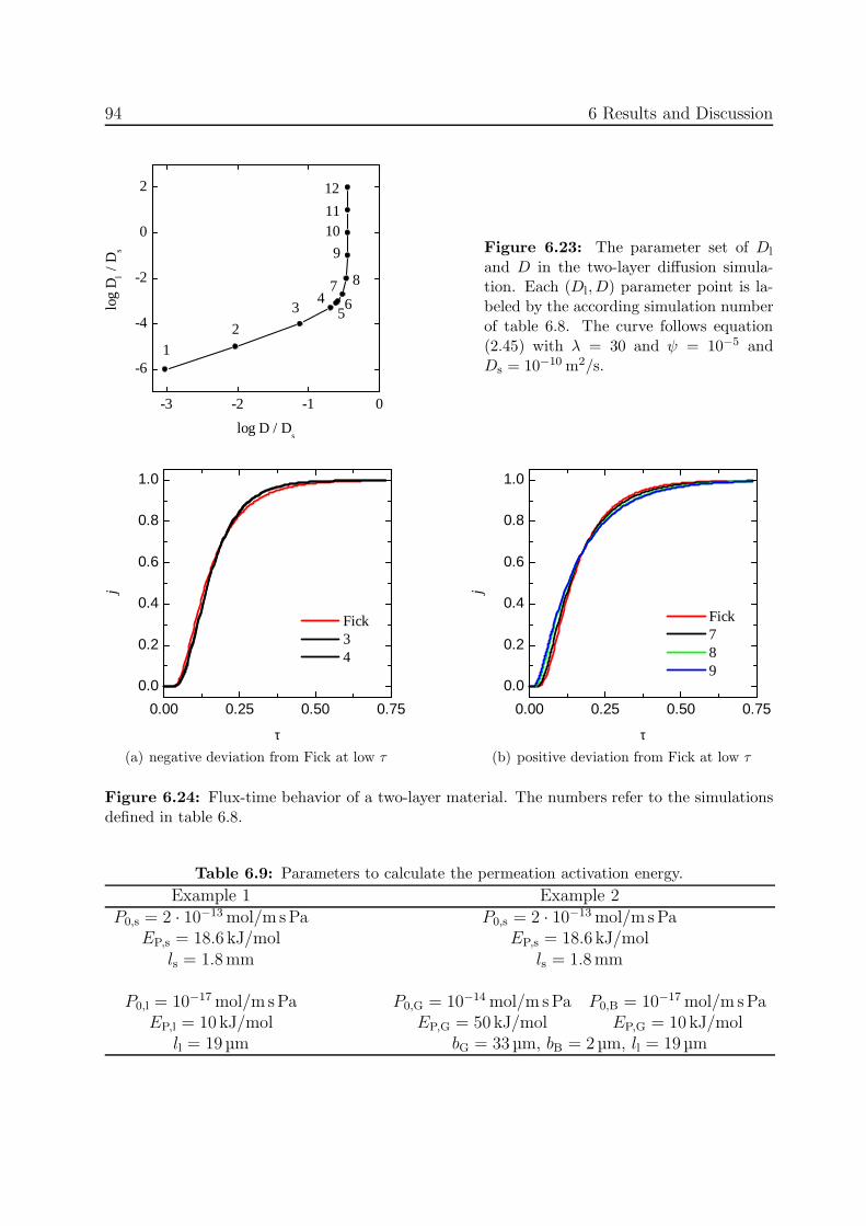
94 6 Results and Discussion
-3 -2 -1 0
-6
-4
-2
0
2 12
1110
9
876
54
3
21
log
Dl /
Ds
log D / Ds
Figure 6.23: The parameter set of Dl
and D in the two-layer diffusion simula-tion. Each (Dl,D) parameter point is la-beled by the according simulation numberof table 6.8. The curve follows equation(2.45) with λ = 30 and ψ = 10−5 andDs = 10−10 m2/s.
0.00 0.25 0.50 0.75
0.0
0.2
0.4
0.6
0.8
1.0
Fick 3 4
j
τ(a) negative deviation from Fick at low τ
0.00 0.25 0.50 0.75
0.0
0.2
0.4
0.6
0.8
1.0
Fick 7 8 9
j
τ(b) positive deviation from Fick at low τ
Figure 6.24: Flux-time behavior of a two-layer material. The numbers refer to the simulationsdefined in table 6.8.
Table 6.9: Parameters to calculate the permeation activation energy.
Example 1 Example 2P0,s = 2 · 10−13 mol/m sPa P0,s = 2 · 10−13 mol/m sPa
EP,s = 18.6 kJ/mol EP,s = 18.6 kJ/molls = 1.8mm ls = 1.8mm
P0,l = 10−17 mol/m sPa P0,G = 10−14 mol/m sPa P0,B = 10−17 mol/m sPaEP,l = 10 kJ/mol EP,G = 50 kJ/mol EP,G = 10 kJ/mol
ll = 19µm bG = 33µm, bB = 2µm, ll = 19µm

6.3 Simulation of Transient Permeation 95
1 2 3 4 5 6 7 8 9 1010-23
10-21
10-19
10-17
10-15
EP,l
EP
Pl
P Ps
P /
mol
/m s P
a
T -1 / 10-3 K-1
500 0 T / °C
10
12
14
16
18
20
EP /
kJ/
mol
(a) example 1
1 2 3 4 5 6 7 8 9 1010-25
1x10-23
1x10-21
1x10-19
10-17
10-15
EP,l
EP
Pl
P
Ps
P /
mol
/m s P
a
T -1 / 10-3 K-1
500 0 T / °C
10
20
30
40
50
60
70
80
EP /
kJ/
mol
(b) example 2
Figure 6.25: Permeation activation energy as a function of the temperature in a 2-layer com-posite. EP is proportional to the negative gradient of the log P (T−1) curve. The parameters ofthe curves are given in the table 6.9.
6.3.3 Simulation of Permeation through Substrates with Defective Liner
The simulations of transient permeation through substrates with a defective liner wereperformed using the model illustrated in figure 6.26. The used model considered two-dimensional diffusion in a homogeneous substrate. Hence, the defects are regarded as linesinstead of holes. The width of the defect and the distance between two defects are denotedin accordance to 2.5.4 by 2 r and 2R, respectively. The liner itself is treated impermeable.The substrate with thickness ls is defined by its transport properties, Ps and Ds. Thepermeability and diffusivity of the composite are denoted by P and D, respectively.
Initial simulations showed that the permeation gas flow through a substrate with adefective liner is less than that without a liner, i. e. the barrier constant was ι < 1. Thebarrier constant was independent from the substrate’s diffusivity/permeability and onlydependent on the geometry. This implies that the permeation activation energy of thecomposite equals that of the substrate:
EP = EP,s.
The diffusivity of the composite of substrate and liner was less than that of the substrate:D < Ds. The j(τ) curve was independent from the material properties of the substrate.
In the following, the j(τ) curves and diffusivities of selected examples are reviewed. Theparameters of the simulations are summarized in table 6.10. The size and the distance ofthe defects were chosen so that they represent expectable coating defects. The simulation 1represents cracks in the liner, the remaining simulations represent greater material defects.

96 6 Results and Discussion
impermeable liner
flux
substrate
fully permeable defect
(a) physical model
Ps, Ds
∂J/∂y = 0∂J/∂y = 0
∂J/∂x
=0
∂J/∂x
=0
C = C0
C = 0
2R
2 r
l s
(b) mathematical model
Figure 6.26: Model to simulate permeation through defectively coated CFRP.
Table 6.10: Simulation parameters of permeation through substrates with defective liner andtheir results.
parameters resultssimu 2 r 2R ls ι ιPrins (2.48) D/Ds j(τ) behaviorno. µm mm mm1 2 0.052 1.4 0.052 0.095 1.00 exact Fickian2 26 72.026 1.8 0.003 2 · 10−5 0.36 not Fickian3 40 1.040 1.8 0.255 0.172 0.66 near Fickian4 40 10.040 1.8 0.041 0.002 0.40 not Fickian5 80 1.080 1.8 0.366 0.346 0.70 near Fickian6 80 10.080 1.8 0.060 0.003 0.42 not Fickian
0 5 100
2
4
6
8
10
12substrate
6, 4, 1, 2
5
3
J /
10-9
mol
/m2 s
t / 104 s
(a) flux as a function of time
0.00 0.25 0.50 0.75
0.0
0.2
0.4
0.6
0.8
1.0
3, 5
substrate, 1
2, 4, 6
j
τ(b) normalized flux as a function of dimension-less time
Figure 6.27: Simulated flux-time behavior of defectively coated CFRP. The labels refer to thesimulation numbers of table 6.10

6.4 Discussion 97
The results of the simulations are presented in table 6.10 and shown in figure 6.27.The reduction of the steady-state flux is remarkable if the defect distance is great. Thediffusivities are in the range 1.9 · 10−11 m2/s and 3.5 · 10−11 m2/s and hence remarkablyless than those of CFRP and similar to those found in the experiments. Figure 6.27-bdisplays the j(τ) curves in comparison to that of Fick. The flux-time curves are similarto the Fick-curve, but a positive deviation in the beginning of the permeation process canbe recognized. The deviations mainly depend on the defect distance. The deviations are,however, not as distinct as found in the experiments, see figure 6.18
Table 6.10 also lists the barrier factor derived from the simulation of Prins & Herman(2.48). The barrier factor of this simulation and that of Prins & Herman agree well forlarge defect size and small defect distances. For small defects being largely separated, thesimulated steady-state flux does not coincide with the results of circular defects.
6.4 Discussion
6.4.1 Permeation through CFRP
The permeation measurements on CFRP specimens revealed deviations of the flux-timecurves from the Fickian theory, see figures 6.5-a and 6.12-a. These deviations were observedin eight of ten investigated CFRP samples. Because the homogeneous PVC specimens didnot show those deviations (see figure 6.2), CFRP can be considered to be inhomogeneous.
It is assumed that highly diffusive paths exist in CFRP which lead to an earlier rise of thepermeation flux. These paths might follow the structure of the reinforcement texture andare in general curved and cross-linked. The following simulation of permeation throughCFRP takes a simpler model into account. Instead of curved and cross-linked paths,parallel paths are employed. In analogy to grain boundary diffusion, the resin and thefibers represent the grain boundary and the grain, respectively.
The diffusivities and widths of the fiber region as well as the resin region were varieduntil the best fit to the experimental j(τ) curve was found. Taking specimen S45c as anexample, figure 6.28 presents the results of the simulation in comparison to the experimen-tal results. The simulated flux-time curve matches exactly the experimental data. Thesimulation was performed with the following parameters
width of fiber region: bG = 0.42mmwidth of resin region: bB = 0.78mmdiffusivity of fiber region: DG = 8.7 · 10−12 m2/sdiffusivity of resin region: DB = 1.74 · 10−10 m2/s.
Considering the width values of the simulation, the fiber volume fraction of S45c wouldbe ff = bG/ (bG + bB) = 35 %. This value is approximately 15 % lower that of the realmaterial. Although the simulations took a simplified model into account, the existence ofhighly-diffusive paths in CFRP would explain the deviations of the j(τ) curves from Fick.

98 6 Results and Discussion
0.00 0.25 0.50 0.75
0.0
0.2
0.4
0.6
0.8
1.0
j
τ
experiment simulation Fick
Figure 6.28: Simulation of the flux-timebehavior of sample S45c. The minor de-viation of the experimental data from theFick distribution can be simulated by theparallel grain boundary model and param-eters as listed in the text.
6.4.2 Permeation through Metal-plated CFRP
The results of the permeation measurements on metal-plated CFRP revealed a great scatterof the total permeability, the activation energy and the j(τ) behavior. In particular, theresults within some material systems varied strongly. Possible explanations are investigatedand discussed in the following, considering the cNiP-Cu plated CFRP specimens of M15.
The RT permeabilities of the M15 specimens varied from from 1.4 · 10−17 mol/m sPa toless than 5.4·10−20 mol/m sPa (see figure 6.15). The activation energies were determined tobe between 14 and 19 kJ/mol. All j(τ) curves showed great deviations from the Fick curve,refer to figure 6.18-b. Assuming a CFRP substrate with nearly constant permeabilities andactivation energies, the high scatter must be caused by a varying coating. The followingexplanations are considered and investigated:
1. strong variation of the liner thickness
2. existence of grain boundary diffusion
3. existence of defects in the coating
4. a combination of the three previous points.
To 1. A variation of the liner thickness was proven during the characterization of thematerials in chapter 4. In polished-cut images of M15, the Cu liner thickness rangedfrom 48 to 59µm (refer to table C.4). Assuming an ideal two-layer permeation process inhomogeneous materials, as described in 2.5.3 and 6.3.2, the total permeability is calculatedby (2.41). Table 6.11 lists the total permeability as a function of the liner permeability forthe two extremes of the liner thickness. The difference of the total permeabilities betweenthese two extremes is always less than 23%. Hence, the scattered results are not causedby a variation of the liner thickness of ±5µm only.
To 2. The existence of grain-like structures was shown in chapter 4. In order to finda possible correlation between the structure of the liner and the measured permeabilities,

6.4 Discussion 99
Table 6.11: Total permeability P as a function of the liner permeability Pl and the liner thicknessll. P is calculated by (2.41) with Ps = 10−16 mol/m s Pa and ls = 1.8 mm.
log Pl -23.00 -22.00 -21.00 -20.00 -19.00 -18.00 -17.00 -16.00ll = 48µm: log P -21.41 -20.41 -19.41 -18.42 -17.43 -16.55 -16.09 -15.99ll = 59µm: log P -21.50 -20.50 -19.50 -18.50 -17.51 -16.62 -16.10 -15.99rel. diff. of P in % 22 22 22 22 21 16 4 0
0.00 0.25 0.50 0.75
0.0
0.2
0.4
0.6
0.8
1.0
j
τ
S08 simulation Fick
Figure 6.29: Simulation of the flux-timebehavior of sample S08. The experimentaldata can be reproduced well by employingthe parallel grain boundary model. Theused parameters wereDB/DG = 100, bB : bG : l ≈ 1 : 1.65 : 9.5.
specimens S10 and S14 were investigated more intensively. While S10 was characterized bya high permeation rate, S14 showed a low permeability. Table 6.12 compares the structureof the liner surface of both specimens. In both samples, circular, grain-like structureswith 25 . . . 50µm in diameter are visible (table 6.12 a,b). At higher magnifications it isrecognizable, that these grain-like structures consist of smaller grains with approximately23 nm for S10 and 20 nm for S14 in diameter (table 6.12 c). EDX line scans along thegrain-like structures revealed similar element distributions in both specimens (table 6.12 e).While the copper content was dominant, that of oxygen was around 5 atom percent. Carboncould be detected proportionally strongly near the boundaries of the grain-like structures.It is assumed that organic dirt accumulates better along these boundaries.
Although no distinctive differences between the liner surfaces of S10 and S14 were foundto understand the enormous deviation of the measured permeabilities, the diffusion throughgrain boundaries would explain the strong deviations of the measured j(τ) curves and thelow activation energies. Figure 6.29 shows the j(τ) curve of S08 in comparison with theFickian distribution and the curve derived from the simulations. Although a substrate isnot considered in the simulations, the trend to reproduce the experimental data with grainboundary diffusion simulation is visible.
To 3. The third possible explanation of the great experimental scatter are defects inthe coating. Therefore, each specimen of M15 and additionally of M17 was inspected moreintensively. Scanning the surface of the liner by means of a stereo microscope and SEM, nouncoated areas were found. Subsequently, the coatings were peeled off, if feasible. Placing

100 6 Results and Discussion
Table 6.12: Comparison of the surface structure of two cNiP-Cu coated CFRP specimens.
S10 S14
(a)surface x100outlens detector
200 µm 200 µm
(b)surface x500outlens detector
100 µm 100 µm
(c)surface x100000inlens detector
500 nm 500 nm
EDX scans across the Cu: 50 . . . 85% Cu: 55 . . . 85%(d) boundaries of grain- C: 12 · · ·50% C: 8 · · · 45%
like structures O: max 5% O: max 10%
(e) P (RT) / (mol/m sPa) 1.38 · 10−18 7.79 · 10−20
EP / (kJ/mol) 16.3 n/a

6.4 Discussion 101
Table 6.13: Correlation between the number of holes (n. o. h.) in the coating of M15 and M17and the measured permeabilities.
M15 (CFRP+cNiP-Cu) M17 (CFRP+cNiP-Ni)sample n. o. h. P (RT)
mol/m sPaEP
kJ/molsample n. o. h. P (RT)
mol/m sPaEP
kJ/molS08 10 7.42 · 10−19 14.2 S30 1 1.85 · 10−19 12.2S10 9 1.38 · 10−18 16.3 S31 4 4.97 · 10−19 15.0S11c 3 5.72 · 10−19 19.3 S32c 0 < 5.48 · 10−20 n/aS13 0 7.38 · 10−20 n/a S33c 0 < 4.29 · 10−20 n/aS14 1 7.79 · 10−20 n/aS15c 1 < 5.44 · 10−20 n/aS16c 1 2.46 · 10−19 n/a
0 2 4 6 8 100
5
10
15 S08 S10 S11c S13 S14 S15c S16c
S30 S31 S32c S33c
P /
10-1
9 m
ol/m
s Pa
number of holes
Figure 6.30: Measured per-meabilities of material systemM15 (S08 – S16c) and M17(S30 – S33c) in correlation tothe number of holes in thecoating. The plotted perme-abilities of S15c, S32c andS33c are the minimum de-tectable signals.
the liners in front of a light, circular holes were found. The number of the found holes aresummarized in table 6.13, although the real number of holes might be even higher. Thediameter of these holes ranged from 26µm to 100µm. Figure 6.30 displays the number ofholes in correlation to the measured permeability. It is well to recognize that the measuredpermeabilities generally increase with the number of holes.
The origin of the holes is explained exemplarily for specimen S08 in figure 6.31. Thesubstrate contained cavernous spots at the same locations where holes were found in thecoating. These cavernous spots in the substrate were also coated but the thickness of thecoating was negligible. In order to understand the existence of caverns in the substrate,a micrograph of specimen S12c was prepared, see figure 6.32. A spherical cavern whichtapers toward the surface is visible. The diameter of the cavern is approximately 210µm.The diameter of the hole in the coating increases from 40µm to 240µm. The micrographreveals that the cavern is located at the resin-richest area. The manufacturer of the CFRPstated, that this hole was very likely caused by an air bubble during the production.

102 6 Results and Discussion
(a) peeled-off coating inback light
2 mm
(b) surface of thepeeled-off coating
2 mm
(c) surface of the sub-strate
500 µm
(d) close-up of one cavernin the substrate
Figure 6.31: Microscope images of sample S08. In the back light, 10 holes are visible in thepeeled-off coating (a). Cavernous spots in the CFRP substrate (c) are located at the samecoordinates as the holes of the coating (b). The caverns are coated (d).
500 µm
close-up
(a) optical microscopy
10 µm
(b) SEM close-up
Figure 6.32: Micrograph of a cavernous spot of S12c. The hole in the coating is crater-likeshaped. The surface of the cavern is coated (b). Note: the black vertical lines are grooves createdduring the polishing with ion beams.

6.4 Discussion 103
impermeable liner
substrate
defect: permeable liner
Figure 6.33: Model of the metal-platedCFRP specimens. The metal plating itselfis treated impermeable. Potentially exist-ing defects of the liner are modeled by alow thickness and grain boundaries.
The micrograph unveils two further important facts. Firstly, the thickness of the coatingon the surface of the cavernous spot is partly as low as 1µm. It is assumed that othercaverns can also contain uncoated areas. Secondly, the hole of the liner follows the shapeof a sinkhole. This implies, that the coating does not to get closed with increasing coatingthickness. Such a behavior is probably caused by flow problems out of the cavern [152].
Knowing about the existence of holes in the coating, the remaining metal-plated CFRPspecimens were investigated again. Only coatings with sufficient thickness (' 40µm) couldbe peeled off from the substrate to be placed in the back light. The coatings of the remainingspecimens were investigated under the microscope. Although it is not known if all holeswere found, the following statements can be given:
• Holes in the coating were found in approximately 50% of the metal-plated specimens.No correlation exists between the coating material and the number of holes.
• In general, the permeability increases with the number of holes in microcrack-free,thick (l ' 30µm) coatings.
• The distribution of holes is statistical, this means no pattern of the holes exists.
• The underlying caverns in the CFRP surface are mainly located in resin-rich areas,i. e. between two filament yarns.
Summarizing, the great scatter of the experimentally determined permeabilities of metalplated CFRP is caused by statistically existing caverns in the CFRP. While the defect-free surface of the CFRP is coated by the nominal thickness, the caverns are insufficientlycoated. A simplified model to explain the permeation through such a body is shown infigure 6.33. The liner on the “perfect” part of the CFRP surface is treated as impermeable.The thin liner at the caverns is permeable and consists of grain boundaries. The permeationthrough the thin part of the liner is responsible for the lower values of EP, compared tothose of uncoated CFRP, and for the remarkable deviations of the measured j(τ) curvesfrom the Fickian distribution.
6.4.3 Evaluation of the Barrier Function of the Liners
All sheets, foils, and foils adhered on CFRP, except those made of Sn, were impermeablewithin the limit of the measuring apparatus. The minimum detection limit varied from

104 6 Results and Discussion
one experiment to the next owing to changing calibration factors and residual pressureswithin the measuring chamber. The lowest liner permeability limits were found in a 25µmCu (S71) and a 30µm Al foil (S72) adhered on CFRP with Pl < 1.9 · 10−22 mol/m sPa, seetable D.3. Considering a CFRP substrate with ls = 1.8mm and Ps = 10−16 mol/m sPa,the barrier constants (2.44) were < 1/7400 and < 1/9100, respectively.
The metal-plated specimens showed very scattered barrier properties, depending on theexistence of holes in the coating. Considering the optimal case of hole-free coatings in S15c,S33c, S46c, S51 and S65, the permeation rates were below the detection limit. The lowestliner permeability limit was found in S46c and S65 with Pl < 8 · 10−22 mol/m sPa. Thepermeation flux through CFRP was reduced at least by factor 7400.
The remaining coatings of M28 (DLC), M29 (thermal spray aluminum) and M30 (PVDNi) did not reduce the permeation flux through CFRP significantly. The barrier constantof M28 was between 0.37 and 0.70 which is still remarkable for an only 2.3µm thick coating.The barrier constants of M29 and M30 were ≈ 1 and 0.44, respectively.
Evaluating the permeation properties and the material characterization from chapter 4of all specimens, metal platings and foils are recommended to use as a permeation barrier.If foils could be joined leak-freely, they were the favored liner.
The determined liner permeabilities are used in the following to estimate the permeationgas flow through the tank system presented in 3.4. Considering (3.4), the steady-statepermeation gas flow would be
QP = 2.339 · 1010 mbar l
s
P
mol/m s Pa
m
l.
Values of P , l and QP are presented in table 6.14 for five liner solutions. The right-most column of this table lists the minimum limit of the vacuum stability time at roomtemperature. In all cases, the maximum limit of the expected gas flow through the CFRPtank is higher than the required maximum allowable gas flow, see (3.3). Hence, in orderto achieve measurement results which can prove the requirement (3.3), specimens with asurface area similar to that of the tank would be required.
Table 6.14: Four possible liner solutions and their permeation properties. The CFRP substrateis represented by ls = 1.8 mm and Ps = 10−16 mol/m s Pa. QP denotes the permeation gas flowthrough the CFRP inner tank. t∗ is the time to reach the maximum allowable vacuum pressure:t∗ = (pv,max Vv) /QP, with pv,max = 5 · 10−4 mbar and Vv = 60 l, see 3.4.
substrate liner ll Pl(RT) P (RT) QP(RT) t∗(RT)µm mol/m sPa mol/m sPa mbar l/s d
CFRP Cu foil 25 < 1.87 · 10−22 < 1.36 · 10−20 < 1.75 · 10−7 > 2.0CFRP Al foil 30 < 1.83 · 10−22 < 1.12 · 10−20 < 1.43 · 10−7 > 2.4CFRP Cu coating 50 < 8.00 · 10−22 < 2.96 · 10−20 < 3.74 · 10−7 > 0.9CFRP Cu coating 100 < 8.00 · 10−22 < 1.52 · 10−20 < 1.87 · 10−7 > 1.9
— Al sheet 1000 < 1.71 · 10−21 < 1.71 · 10−21 < 4.00 · 10−8 > 8.7

Chapter 7
Conclusions
“Basic research is like shooting an arrow into the air and,where it lands, painting a target.” Homer Burton Adkins
Summary
The objective of this thesis was to find an appropriate liner for the inner shell of an LH2
tank made of CFRP. The liner — located at the outside surface of the shell — is requiredto prevent permeation of hydrogen through and outgassing from the inner tank into theinsulating vacuum. Although outgassing was taken into account, too, the main objectivewas the permeation measurement of various liner types.
Surveying the outgassing rates and permeabilities from literature, only few metals andglasses satisfy the high requirements for the liners to enable a stable vacuum. Possibleproduction processes to apply those materials on CFRP were studied and evaluated. Themaximum allowable temperature of CFRP (≈ 120 . . . 140 °C) and the applicability on thelarge and from-adapted structure of the LH2 tank restricted the number of feasible pro-cesses. The chosen liner materials and production processes were
• Foils/sheets: Al, Cu, Sn and SS
• Metal platings with cNiP starting layer: Al, Au, Cu, Sn, and Ni
• Metal platings with cCu starting layer: Cu, Au and Sn
• Thermal spray Al
• PVD: C (DLC) and Ni.
All material tests and investigations were performed on flat specimens (plates, discs). Ex-cept for sheets and some of the foils, all liners were applied on CFRP substrates.
Besides permeation tests, the investigation of the various liners included the charac-terization by means of SEM, thermal shock experiments and adhesive strength tests. Thepermeation measurements were performed in two separate apparatuses, working between293K and 373K (RTPMA) and between 20K and 293K (CPMA), respectively. Bothapparatuses were designed and built to investigate CFRP, metals or the combination ofboth. The transmission method was used to imitate the real load case of the tank asgood as possible. Feeding the test gas at one side of the specimen, the molecules permeatethrough the membrane into a flowing stream. There, the partial pressure of the permeating
105

106 7 Conclusions
gas was measured by means of a mass spectrometer and subsequently converted into thecorresponding permeation rate.
The relationship between measured pressure and permeation flux was found by cali-brating the mass spectrometer instead of using the constant pumping speed. The acquiredcalibration factors varied statistically around a mean value. Considering long terms, themean value increased gradually by time. This increase was found to originate from adegradation of the filaments. Within one year, the sensitivity of the mass spectrometerdecreased by factor 10. Hence, an error of 1000% or more is possible if the speed of theturbomolecular pump is used instead of a calibration factor.
A typical permeation test consisted of the assembly of the specimen, the permeationmeasurement and the disassembly. During the assembly, an indium wire was squeezedbetween the specimen and two specimen holders to enable a leak-free sealing. This processwas very critical and could not be successfully performed for every specimen. Mainly arough surface of the specimen or mechanically weak liners were reasons for failing seals.After the subsequent bake-out at approximately 120 °C for 24 hours, the calibration wascarried out. The actual permeation measurements were started at room temperature.Depending on the material, the steady-state permeation flux was typically reached afterone or two days — if permeation was measurable at all. The change in temperature resultedin a change of the flux approaching a new steady-state within few hours. In very few cases,leaks in the sealing occurred during the change of the temperature.
Initial permeation tests were carried out to prove the functionality and reliability ofboth apparatuses. The measurements on CFRP and PVC showed consistent results at theRTPMA and CPMA. The permeabilities agreed well with those from the literature. Theinitial tests also revealed disadvantages of hydrogen as a test gas. The minimum detectablesignal of hydrogen was almost four orders of magnitude higher than that of helium. Fur-thermore, hydrogen permeation was strongly influenced by environmental factors like thedaily sunshine durance or the temperature. It is believed that the adsorption and releaseof hydrogen in the stainless steel chambers is very sensitive to the temperature and causeserrors in the measurement. Because the permeabilities of helium and hydrogen were foundto be similar in seven specimens, helium was used as test gas in the following.
Important for the quality of the measurement results is the minimum detectable gasflow. The minimum detectable gas flow is the product of the minimum detectable pres-sure and the calibration factor. Both factors can vary from one experiment to the other,depending on the material of the specimen, the quality of the sealing, and the state of themass spectrometer’s filaments. The typical limit of the detectable He gas flow was between4 · 10−11 and 5 · 10−10 mbar l/s. Related to the permeating area of the RTPMA specimens,the minimum detectable area-specific gas flow was between 1·10−8 and 1.2·10−7 mbar l/sm2.In order to prove the requirement of the maximum allowable area-specific permeation gasflow through the tank vessel at room temperature (3.3), q < 1.5 · 10−10 mbar l/sm2, thesensibility of the measuring apparatus would have to be between 66 and 800 times bet-ter. Hence, the employed measurement apparatuses enabled a comparison of the singleliners and a general qualification/feasibility of them. In order to quantitatively prove therequirements, tests on specimens as large as the tank are necessary. On the other hand,

7 Conclusions 107
considering the best minimum detectable signal (1·10−8 mbar l/sm2) ever measured, a tankvacuum stability time at room temperature of more than 56 days is feasible to prove.
Evaluating the results of the permeation measurements together with those of the ad-hesive strength and thermal shock tests, the foil/sheet liners and metal platings exhibitedthe highest potentials. Still, both liner types face some to-be solved challenges.
The structure of foils and sheets was compact and defect-free, which is characteristicfor the production process (rolling, extrusion). The adhesive strength of some foils onCFRP was too low which resulted in a partial peeling. With the exception of tin speci-mens, the permeation gas flow through foils and sheets was lower than the detection limit.Remarkably, a 25µm Cu foil adhered on CFRP and three welded, 1mm thick Al sheets didnot allow any measurable permeation. Considering the 25µm Cu foil, the permeation fluxthrough the protected CFRP was reduced at least by factor 7400 compared to CFRP. Themeasured He permeability of copper was less than 2 · 10−22 mol/m sPa. Introducing sheetsor foils as a liner on a free-form CFRP inner tank, the application of them would require aleak-free joining method with low heat production. This issue was not investigated in thisthesis.
In contrast to foils, full metal platings can be produced on the outside of an inner LH2
tank vessel. The investigated metal platings consisted of at least two layers. The first layerwas produced by chemical deposition of copper or nickel. The typical thickness of this initiallayer was between 1 and 10µm. Subsequently, the functional layer was applied by eitherchemical or electrochemical deposition. The materials of the functional layers were copper,nickel, gold, tin and aluminum. Depending on the material and the process parameters,the coatings contained grain-like structures on the surface. While the diameter of thesegrain-like structures was only 1 – 3µm for chemical copper, those of aluminum were upto 160µm in diameter. The coatings consisting of chemical nickel contained cracks whichcan be explained by their brittleness. Tin coatings were fully traversed by cracks afterthermal shock which was ascribed to the phase transition at 286K. The gold layers, havinga thickness of only few micrometers, were not fully deposited but contained holes. Thealuminum liners either exhibited uncoated spots or channels. Some of the metal platings,independent from the material and thickness, were characterized by circular holes. Theseholes, being maximal 100µm in diameter, originated from defects (voids, caverns) on thesurface of the substrate. The caverns on the CFRP surface were only coated by materialfew micrometers thick or not at all. The existence of holes had a substantial impact on themeasured permeabilities. Functional liners made of nickel sulfamate or copper containingno holes were impermeable within the accuracy of the measurements. In this case, thepermeation gas flow through CFRP was reduced by more than factor 7400 (S46c, S65). Onthe contrary, a copper coating with nine holes (S10) reduced the permeation flux throughCFRP only by factor 67. It was shown that — independent from the coating material —the total permeability is approximately proportional to the number of holes.
Temperature-dependent permeation measurements on metal-plated and uncoated CFRPspecimens were performed between 20K and 373K. The measured permeation flux gener-ally decreased with decreasing temperature. For temperatures below approximately 200K,

108 7 Conclusions
no permeation could be detected in all investigated specimens. In particular, no perme-ation gas flow could be measured at 20K. The extrapolated permeability of uncoated CFRP(worst case) at 20K is 5 · 10−62 mol/m sPa.
In some specimens containing either a cNiP, cNiP-cAu or cNiP-Sn coating, suddenand short increases of the permeation flux were recorded during the cooling phase. Thesubsequent measurement at RT revealed an increase of the permeation rate to values ofuncoated CFRP. Hence, the peaks of the flux resulted from the formation of cracks in theaccording liners. Specimens with a copper or nickel functional layer did not show any peaksand did not form microcracks during cooling.
The measured activation energies of permeation through metal-plated CFRP were be-tween 7 and 20 kJ/mol, but mostly below 15 kJ/mol. These activation energies are lowerthan those of uncoated CFRP (18 ± 1 kJ/mol). Simulations and calculations proved, thatthis behavior only occurs if the activation energy of permeation through the liner is low.Permeation though CFRP with an impermeable but defective coating would result in thesame activation energy as uncoated CFRP. The low activation energy of the coating isassumed to be caused by grain boundary diffusion.
The assumption of grain boundary diffusion is emphasized by transient simulations per-formed with a self-written Matlab program. The aim of the simulations was to understandthe various existing flux-time curves obtained from the experiments. In particular, somemeasured j(τ) curves showed strong deviations from the Fickian curve, which describes per-meation through a homogeneous material. Three models were employed: grain boundarydiffusion, permeation through two homogeneous layers and permeation through a substratewith a defective liner. The parameters of the simulations were chosen to reflect the exper-iments as good as possible. Neither the simulation of two-layer permeation nor those ofpermeation through defectively coated CFRP could reproduce the j(τ) curves found in theexperiments. On the contrary, the simulation of grain boundary diffusion could describethe j(τ) shape obtained from the experiments. It was found that the deviations from theFickian curve depend on the size of the boundaries, the distance between those and theratio between the grain and grain boundary diffusivity.
Considering the scattering in the values of the permeabilities, the low activation en-ergies, and the partly found strong deviations of the j(τ) curve from the Fickian curve,the permeation through metal-plated CFRP specimens can be described as followed: Aclosed, defect-free metal plating is impermeable for helium. If defects in the coating orvery low coating thicknesses exist, then the barrier function of the coating is reduced. Thepermeation through these coating defects with low thickness is dominated by grain bound-ary diffusion. The existence of grain boundaries additionally justifies the usage of heliuminstead of hydrogen. In grain boundaries, vacancy diffusion is assumed to be present andresults in a similar diffusion behavior of He and H2.
Besides sheets/foils and metal platings, thermal spray aluminum and physical vapordeposited carbon and nickel coatings were investigated. The three latter coatings didnot reduce the permeation flux dramatically. While the PVD Ni and the DLC coatingscontained cracks presumably owing to high internal stresses, the thermally sprayed Alcoating did not form a closed layer.

7 Conclusions 109
Evaluating and comparing the permeation properties, sheets/foils and defect-free metalplatings enabled a reduction of the permeation flux through CFRP below the minimumdetection limit. Using this detection limit to calculate the stability time of the insulatingtank vacuum, only a lower limit of the time can be given. At room temperature, a 30µmAl foil, a 25µm Cu foil or a 100µm Cu metal plating would enable a vacuum stabilityfor at least 2 days. An aluminum sheet with 1 mm in thickness would even increase theminimum expectable time to 9 days. At 20 K, no reasonable permeation is expected.
The results of this work were used to choose an appropriate liner for the CFRP innertank introduced in chapter 1. Considering and evaluating all properties of the variousliners, the CFRP tank was coated by means of metal plating (see figure of the title page).The coating consisted of a chemical copper layer, followed by an electrochemical copperlayer. Although the tank was fully coated, permeation tests could not be performed owingto predominating leaks in the CFRP structure.
Summarizing, a promising liner material and the according production process werefound to prevent permeation through CFRP at temperatures between 20 and 373K. Thefinal qualification of this liner, however, must be performed on a tank itself.
Future Work
This work has shown that metallic liners are feasible to apply on CFRP and to reduce thepermeation rate below the detection limit. Still, there is a lot of space for improvementsand future work.
The minimum detection limit of the measurements was too high to present results thatcan prove the tank requirements for the vacuum stability. An improvement can be achievedby either using larger specimens or applying higher feed pressures. When increasing the feedpressure, the limited ultimate strength of the specimens and the sensitivity of the sealingmust be considered. Larger specimens are more difficult to seal, especially when measuringat varying temperatures. The lower stiffness and strength of larger specimens must also betaken into account. The usage of tubes instead of flat specimens would be an alternative.A promising approach to enhance the sensitivity of the mass spectrometer is given by Firpoand Pozzo [153]. There, the pumping speed of the gas of interest is reduced, while all othergases are evacuated constantly. Employing this method, the minimum detectable signalcould be reduced by factor 10.
It was shown, that electroplatings on CFRP can be a permeation barrier if they do notcontain defects. This implies that the surface of the CFRP must be free of caverns. Studieson the CFRP production process could indicate and subsequently prevent factors that favorthe formation of those caverns. A promising approach is the usage of the resin transfermolding (RTM) process instead of the VARI process. In the RTM process, air enclosuresare more present within the CFRP but less near the surface [154]. At the end of thiswork, four 200×100mm2 CFRP plates were produced by means of RTM and subsequentlycoated by 50µm copper. Only one hole was found in the four liners having an area of800 cm2. Additionally to the improvement of the CFRP surface, the coating process can

110 7 Conclusions
be further investigated. Emphasis should be laid on understanding why caverns cannot befully coated with increasing liner thickness.
All tests were performed on flat, nearly perfect specimens. However, the producedfree-form CFRP tank contained leaks which were probably formed owing to different loadcases and/or imperfections in the CFRP. Presuming an always existing potential of leakagein the CFRP structure, the size of the cracks causing this leakage should be determined.Subsequently, the ability to cover these cracks by coating should be investigated. Anotheroption is a liner consisting of two layers. The first layer is very ductile, insensitive tothermal shocks or mechanical loads, and does not form cracks. Hence, this layer shall workas a crack stopper and prevent leakage. The second layer consists of a liner presented inthis work and prevents permeation and outgassing.
Foils showed a great potential as a permeation barrier. However, leak-free joining meth-ods must be found to employ foils as a liner. Processes like welding (high temperatures)or adhering (leakage) are not feasible. An alternative solution would be the application ofsingle foil parts and the subsequent coating of the joining lines.
The qualification of the liners also requires the measurement of their outgassing rates.In order to be able to prove very low outgassing rates, large specimens — preferably thetank itself — should be used. The influence of the bake-out temperature and bake-outtime can be determined by sensitivity studies. Cleaning methods, like chemical or glowdischarge cleaning, should be investigated to further reduce the outgassing rate.

Appendix A
Literature Survey of H2 Permeabilities
Table A.1: Permeabilities of metals. P0 and P in mol/m s Pa0.5, EP in kJ/mol.
metal P0 EP T / K P (293 K) ref.Ag 8.51E-07 100 887-998 1.24E-24 [155]Al 5.80E-05 123 400-800 6.70E-27 [156]Al 2.46E-04 129 200-500 2.84E-27 [157]Al 3.98E-05 121 833-998 1.28E-26 [155]Al 1.00E-09 52 400-800 4.38E-19 [38]Al 3.30E-10 97 1273-1673 1.41E-27 [158]Al 5.80E-05 123 420-520 6.70E-27 [159]Al 5.20E-05 121 666-994 1.62E-26 [43]Al oxidized 1.01E-09 52 733-823 4.44E-19 [160]Al oxidized 7.50E-14 823 [160]Al oxidized 1.61E-10 54 763-823 4.34E-20 [160]Al oxidized 6.04E-10 57 683-738 4.01E-20 [160]Al oxidized 5.48E-11 46 763-823 3.04E-19 [160]Al oxidized 4.36E-11 42 763-823 1.41E-18 [160]Al oxidized 1.86E-09 77 793-823 3.06E-23 [160]Al oxidized 1.26E-10 54 763-823 2.85E-20 [160]Al2O3 8.82E-02 322 1459-1721 2.82E-59 [161]Al 2.00E-26 300 2.00E-26 [162]Au 1.98E-06 115 300-640 6.23E-27 [163]Au 1.89E-03 171 967-998 6.33E-34 [155]Au 1.14E-06 115 400-800 3.59E-27 [38]Au 3.10E-06 123 500-900 3.58E-28 [159]Be 5.80E-14 18 670-1170 3.18E-17 [159]Co 6.30E-09 57 400-670 4.43E-19 [159]Cu 5.50E-07 75 623-973 2.51E-20 [164]Cu 1.34E-07 63 1075-1172 8.51E-19 [165]Cu 1.28E-07 72 200-500 1.72E-20 [157]Cu 7.05E-07 76 684-998 1.93E-20 [155]Cu 8.40E-07 77 1.33E-20 [38]Cu 1.10E-05 98 9.90E-19 [166]Cu 8.40E-07 77 470-700 1.29E-20 [159]
111

112 A Literature Survey of H2 Permeabilities
metal P0 EP T / K P (293 K) ref.Cu 7.18E-09 61 667-997 1.12E-19 [43]Fe 1.99E-07 39 628-681 1.45E-12 [34]Fe 4.90E-05 35 623-973 2.92E-14 [164]Fe 2.09E-06 35 200-500 1.43E-12 [157]Fe 4.03E-08 35 625-1002 2.47E-14 [155]Fe 5.72E-08 37 355-645 1.54E-14 [73]Fe 4.10E-08 35 375-500 2.44E-14 [159]Fe 5.35E-08 34 5.48E-14 [38]Ge 1.20E-05 200 1040-1200 3.20E-41 [159]Mo 2.30E-07 81 500-1700 9.32E-22 [159]Mo 8.05E-09 48 666-994 2.10E-17 [43]Nb 6.50E-09 -29 692-1000 9.55E-04 [155]Nb 6.30E-09 -36 700-1000 1.34E-02 [159]Nb 1.53E-08 5 751-995 2.32E-09 [43]Ni 4.40E-07 55 673-1123 7.19E-17 [164]Ni 1.28E-06 59 200-500 4.73E-17 [157]Ni 3.17E-07 55 418-773 5.70E-17 [167]Ni 9.62E-08 63 4.53E-16 [166]Ni 6.16E-07 58 396-722 2.95E-17 [73]Ni 4.00E-07 55 300-775 6.60E-17 [159]Ni 8.40E-08 49 313-455 1.41E-16 [98]Pd 3.33E-07 15 285-667 7.81E-10 [168]Pd 2.16E-07 16 574-1165 3.55E-10 [169]Pd 1.12E-07 13 624-1150 5.82E-10 [165]Pd 4.08E-07 17 623-1173 4.33E-10 [170]Pd 1.89E-07 15 625-998 4.29E-10 [155]Pd 2.20E-07 16 300-709 3.54E-10 [159]Pd 1.34E-07 14 667-994 4.69E-10 [43]Pt 5.41E-08 64 709-1000 2.35E-19 [155]Pt 1.20E-07 71 540-900 3.02E-20 [159]Ta 5.46E-09 -21 625-998 2.86E-05 [155]Ta 5.80E-09 -20 625-944 2.32E-05 [159]Ti 4.86E-05 49 666-945 8.13E-14 [43]V 4.90E-06 3 2.04E-06 [166]V 4.00E-09 -25 600-900 1.08E-04 [159]V 1.94E-04 59 667-912 5.07E-15 [43]W 1.47E-09 80 873-1072 7.31E-24 [171]W 7.80E-07 141 1100-2400 4.94E-32 [159]W 1.61E-06 129 839-997 1.62E-29 [43]Y 3.61E-09 -26 625-998 1.42E-04 [155]

A Literature Survey of H2 Permeabilities 113
Table A.2: Permeabilities of stainless steels. P0 and P in mol/m s Pa0.5, EP in kJ/mol.
stainless steel P0 EP T / K P (293 K) ref.Eurofer 97 4.08E-08 40 473-673 2.50E-15 [171]stainless steel 1.20E-07 60 423-700 2.62E-18 [39]stainless steel 2.80E-07 65 473-703 6.48E-19 [39]stainless steel 5.40E-08 56 373-623 5.39E-18 [39]SS 300 series 4.10E-08 60 6.82E-19 [156]SS 303 3.60E-07 67 773-1173 3.53E-19 [164]SS 304 4.99E-08 55 392-650 6.48E-18 [98]SS 304 5.10E-07 71 823-1173 1.28E-19 [164]SS 309S 1.20E-07 59 425-875 3.59E-18 [159]SS 316 2.36E-07 63 416-1018 1.13E-18 [172]SS 316L 3.90E-07 64 1.46E-18 [38]SS 321 5.53E-08 59 497-933 1.42E-18 [172]SS 403 5.90E-08 43 1.44E-15 [38]SS 430 1.12E-07 46 796-1118 5.86E-16 [173]stainless steel 2.47E-07 63 668-1000 1.37E-18 [43]
Table A.3: Permeabilities of nickel alloys. P0 and P in mol/m s Pa0.5, EP in kJ/mol.
nickel alloy P0 EP T / K P (293 K) ref.ANL-1 1.50E-05 65 973-1173 5.96E-17 [170]Haynes 2.12E-07 63 500-1000 1.73E-18 [159]Inconel 1.45E-09 41 313-455 7.87E-17 [98]Inconel 9.30E-07 69 773-1173 5.44E-19 [164]Inconel 600 6.40E-08 48 873-1173 2.23E-16 [170]Inconel 600 3.99E-08 57 423-673 3.72E-18 [36]Inconel 625 2.57E-07 60 423-1007 6.55E-18 [172]Inconel 718 9.59E-08 56 364-1051 1.13E-17 [172]Monel 6.97E-07 52 313-423 5.39E-16 [98]Monel 1.87E-07 53 723-1223 6.10E-17 [164]

114 A Literature Survey of H2 Permeabilities
Table A.4: Permeabilities of iron alloys. P0 and P in mol/m s Pa0.5, EP in kJ/mol.
iron alloy P0 EP T / K P (293 K) ref.52 Alloy 2.79E-10 37 357-588 7.31E-17 [98]Cold-drawn steel 4.70E-08 36 573-873 1.99E-14 [164]iron alloy 8.09E-08 37 667-992 2.28E-14 [43]Kovar 4.67E-09 44 373-666 5.68E-17 [98]Kovar Interpolated 4.56E-07 69 641-998 2.14E-19 [155]mild steel 4.10E-08 35 2.44E-14 [156]Steal 4130 2.91E-08 40 350-900 2.23E-15 [159]
Table A.5: Permeabilities of various alloys. P0 and P in mol/m s Pa0.5, EP in kJ/mol.
alloy P0 EP T / K P (293 K) ref.Cu0.2Pd0.8 1.22E-07 21 627-1160 2.13E-11 [165]Cu0.47Pd0.53 4.15E-08 28 623-1172 4.20E-13 [165]Fe(321-SS)1.3mm+4µm Al 3.42E-09 59 473-923 9.05E-20 [174]Fe0.98Al0.02 (430-SS) and oxidation 2.34E-09 58 626-1112 9.70E-20 [174]Fe0.98Al0.02 (430-SS) 3.40E-09 51 530-1115 2.78E-18 [174]Hf36Ni64 3.00E-08 21 473-623 5.41E-12 [175]Pd0.92Al0.08 partially oxidized 2.57E-09 13 423-504 1.49E-11 [176]V-10mol%Al 3.67E-08 -7 523-624 7.64E-07 [177]V-20mol%Al 5.46E-09 -10 523-624 3.95E-07 [177]V-25mol%Al 4.62E-08 9 523-624 1.06E-09 [177]V-30mol%Al 4.71E-08 18 523-624 2.52E-11 [177]Zr36Ni64 8.00E-08 17 473-623 7.45E-11 [175]Zr36Ni64(0.2) Ti39Ni61(0.8) 6.00E-08 26 473-623 1.39E-12 [175]
Table A.6: Permeabilities of glasses. P0 and P in mol/m s Pa, EP in kJ/mol.
glass P0 EP T / K P (293 K) ref.glass 4.86E-14 34 273-973 4.37E-20 [159]glass 1.29E-13 60 273-973 2.94E-24 [159]glass 2.86E-13 51 273-973 2.79E-22 [159]Pyrex 8.20E-14 26 192-493 1.95E-18 [178]Pyrex 7.67E-14 45 274-1246 8.44E-22 [30]Quarzglas 5.08E-14 33 273-1246 5.65E-20 [30]Zellglas 4.46E-16 293 4.46E-16 [92]Zellglas, polymerlackiert 8.93E-17 293 8.93E-17 [92]

A Literature Survey of H2 Permeabilities 115
Table A.7: Permeabilities of thermoplastics. P0 and P in mol/m s Pa, EP in kJ/mol.
thermoplastic P0 EP T / K P (293 K) ref.ASA 2.55E-15 296 2.55E-15 [91]CTFE 8.60E-11 32 257-343 1.75E-16 [91]CTFE 6.69E-16 293 6.69E-16 [92]ECTFE 2.85E-10 33 251-341 4.51E-16 [91]EDPM 1.12E-10 24 317-349 5.02E-15 [47]FEP 4.46E-15 298 4.46E-15 [179]FEP 9.23E-11 27 257-341 1.70E-15 [91]HDPE 9.13E-11 28 296 8.98E-16 [150]HDPE 1.11E-10 29 255-341 8.09E-16 [91]HDPE 1.12E-15 293 1.12E-15 [92]HDPE 8.07E-16 298 8.07E-16 [180]LDPE 3.57E-15 298 3.57E-15 [93]LDPE 2.45E-15 293 2.45E-15 [92]Noryl 8.66E-13 12 291-343 5.55E-15 [47]PA 12 6.69E-16 293 6.69E-16 [92]PA 12 7.30E-12 26 296 1.42E-16 [150]PA 6 2.23E-16 293 2.23E-16 [92]Parylene 1.07E-15 298 1.07E-15 [91]PBT 6.69E-16 298 6.69E-16 [181]PC 4.90E-11 23 224 4.27E-15 [112]PC 8.93E-15 293 8.93E-15 [92]PC 4.01E-15 298 4.01E-15 [182]PE 1.07E-15 293 1.07E-15 [90]PET 1.82E-16 298 1.82E-16 [183]PET 1.98E-16 298 1.98E-16 [91]PETP 1.79E-16 293 1.79E-16 [92]PI 4.46E-16 298 4.46E-16 [184]PP 2.66E-15 293 2.66E-15 [90]PP 2.90E-15 293 2.90E-15 [92]PP 1.34E-14 298 1.34E-14 [94]PPS 8.31E-16 297 8.31E-16 [91]PS 6.69E-15 293 6.69E-15 [92]PS 7.58E-15 298 7.58E-15 [185]PSU 3.56E-15 296 3.56E-15 [91]PTFE 3.12E-15 298 3.12E-15 [186]PTFE 3.44E-12 17 347-433 3.62E-15 [47]PVC 3.92E-16 293 3.92E-16 [90]PVC 3.57E-16 293 3.57E-16 [92]PVC 2.33E-11 20 296 6.92E-15 [150]

116 A Literature Survey of H2 Permeabilities
thermoplastic P0 EP T / K P (293 K) ref.PVC 1.34E-16 298 1.34E-16 [95]PVC-E 4.46E-16 293 4.46E-16 [92]PVDC 2.68E-16 293 2.68E-16 [92]PVDF 9.74E-17 293 9.74E-17 [90]PVDF 1.34E-16 293 1.34E-16 [92]PVDF 1.07E-16 296 1.07E-16 [91]PVDF 1.12E-16 298 1.12E-16 [187]PVF 1.41E-16 298 1.41E-16 [188]Santoprene 4.96E-13 25 293-333 1.66E-17 [47]TFE 1.40E-11 20 255-341 3.49E-15 [91]UPVC 5.25E-16 298 5.25E-16 [189]UPVC 6.69E-16 298 6.69E-16 [190]
Table A.8: Permeabilities of thermosets. P0 and P in mol/m s Pa, EP in kJ/mol.
thermoset P0 EP T / K P (293 K) ref.CFEP (60%) 8.0E-12 26 200-300 1.9E-16 [150]EP 5.6E-11 28 200-300 5.7E-16 [150]EP 2.2E-16 298 2.2E-16 [91]GFEP (56%) 5.9E-12 26 200-300 1.4E-16 [150]GFRP 4.6E-17 308 4.6E-17 [191]Polypyrrole 3.5E-16 296 3.5E-16 [91]PUR 2.0E-15 293 2.0E-15 [91]IM7/BMI 8.0E-17 293 8.0E-17 [192]
Table A.9: Permeabilities of elastomers. P0 and P in mol/m s Pa, EP in kJ/mol.
elastomer P0 EP T / K P (293 K) ref.CA, 2.5-Acetat 2.32E-15 293 2.32E-15 [92]Kautschukhydrochlorid 1.79E-15 293 1.79E-15 [92]Silicone 1.78E-13 298 1.78E-13 [193]Silicone 8.90E-14 298 8.90E-14 [91]Viton 7.06E-08 47.7 336-402 2.21E-16 [47]

A Literature Survey of H2 Permeabilities 117
1.0 1.5 2.0 2.5 3.0 3.5 4.0 4.5 5.01x10-39
1x10-34
1x10-29
1x10-24
1x10-19
1x10-14
1x10⁻⁹
green symbols: Cublue symbols: Aured symbols: Al
P /
(m
ol/m
s P
a0.5 )
T -1 / (10-3 K-1)
800600 400 200 0T / °C
Figure A.1: Hydrogen permeabilities of copper, gold and aluminum from literature. The dataof table A.1 is plotted.

118 A Literature Survey of H2 Permeabilities
0.5 1.0 1.5 2.0 2.5 3.01x10⁻¹⁶
1x10-11
1x10⁻⁶
Ag Be Co Ge Mo Pt W
Nb Ta Ti V Y Pd
P /
(m
ol/m
s P
a0.5 )
T -1 / (10-3 K-1)
20001750150012501000 750 500 2501000 2000
T / °C
Figure A.2: Hydrogen permeabilities of silver, beryllium, cobalt, germanium, molydenum, plat-inum, tungsten, niobium, tantalum, titanium, vanadium, yttrium and palladium. The data oftable A.1 is plotted.

A Literature Survey of H2 Permeabilities 119
1.0 1.5 2.0 2.5 3.0 3.5 4.0 4.5 5.01x10⁻²²
1x10-21
1x10-20
1x10-19
1x10-18
1x10-17
1x10-16
1x10-15
1x10-14
1x10-13
1x10-12
1x10-11
1x10⁻¹⁰
1x10⁻⁹
1x10⁻⁸
1x10⁻⁷
Fe Ni 52 alloy iron alloy Kovar Kovar Kovar mild steel 4130
ANL-1 Haynes Inconel Inconel 600 Inconel 600 Inconel 625 Monel stainless steel stainless steel SS 304 SS 309S SS 316
P /
(m
ol/m
s P
a0.5 )
T -1 / (10-3 K-1)
800600 400 200 0T / °C
Figure A.3: Hydrogen permeabilities of iron, nickel and their alloys. The data of Fe (green)and Ni (light blue) are taken from table A.1. The data of stainless steel (dark blue), nickel alloy(red) and iron alloy (black) are taken from table A.2, table A.3 and table A.4, respectively.

120 A Literature Survey of H2 Permeabilities
1.0 1.5 2.0 2.5 3.0 3.5 4.0 4.5 5.01x10⁻²³
1x10-22
1x10-21
1x10-20
1x10-19
1x10-18
1x10-17
1x10-16
1x10-15
1x10-14
glass (Steward1983) glass (Steward1983) Pyrex (Rogers1954) Pyrex (Wutz1988) quarz glass (Wutz1988) Zellglas (Saechtling1989) Zellglas (Saechtling1989)
P /
(m
ol/m
s P
a)
T -1 / (10-3 K-1)
1000750 500 250 01001000
T / °C
Figure A.4: Hydrogen permeabilities of glasses. The data are taken from table A.6.

A Literature Survey of H2 Permeabilities 121
2.5 3.0 3.5 4.0 4.5 5.01x10⁻¹⁹
1x10-18
1x10-17
1x10-16
1x10-15
1x10-14
1x10-13
1x10-12
1x10-11
1x10⁻¹⁰
green symbols: thermoplasticsblue symbols: elastomersred symbols: thermosets
P /
(m
ol/m
s P
a)
T -1 / (10-3 K-1)
150 100 50 0 -50T / °C
Figure A.5: Hydrogen permeabilities of polymers. The data of thermoplastics (green), ther-mosets (red) and elastomers (blue) are taken from table A.7, table A.8 and table A.9, respectively.

122 A Literature Survey of H2 Permeabilities

Appendix B
Literature Survey of Outgassing Rates
If not noted, the outgassing rates, qG, are measured at room temperature (RT). The unitof the area specific outgassing rates is mbar l s−1 m−2. The term “xxh at yyy °C” denotesthe bake-out at yyy °C for xxhours.
Table B.1: Area specific outgassing rates of stainless steels
material preparation / treatment qG ref.SS 1 h at RT 2.8E-05 [30]SS 1 h at RT 4.2E-05 [30]SS 1 h at RT 7.1E-05 [30]SS 1 h at RT 8.3E-05 [30]SS 1 h at RT 1.4E-04 [30]SS 1 h at RT 9.0E-04 [30]SS 1 h at RT 3.1E-03 [30]SS 2 h at RT 7.7E-06 [129]SS 2 h at RT 6.3E-05 [194]SS 5 h at RT 1.0E-04 [195]SS 10 h at RT 1.0E-05 [96]SS 20 h at 150 °C 8.4E-07 [128]SS 21 h at 200 °C 1.3E-10 [196]SS 22 h at 212 °C 1.0E-10 [196]SS 100 h at 430 °C, 100 h at 480 °C 3.0E-12 [196]SS electropolished 3.0E-08 [197]SS electropolished, 1 h at RT 4.3E-05 [30]SS mechanically polished, 1 h at RT 1.7E-05 [30]SS sand-blasted, 1 h at RT 8.3E-05 [30]SS (304) 30 h at 250 °C 4.0E-08 [96]SS (304) baked and cleaned 1.3E-08 [198]SS (304) oxidized (3.5 nm CrOxide) 1.6E-10 [199]SS (304) venting with N2, 8 h at 180 °C 2.0E-09 [200]SS (316) baked and cleaned 1.3E-08 [198]SS (316L) 10 h at 20 °C, 40 h at 140 °C, 50 h at 20 °C 7.7E-09 [201]SS (401) 24 h at 300 °C 2.4E-07 [120]SS (U15C) 45 h at 360 °C 1.9E-08 [126]SS (U15C) baked in situ at 360 °C for 24 h 3.7E-10 [126]
123

124 B Literature Survey of Outgassing Rates
Table B.2: Area specific outgassing rates of Al
material preparation / treatment qG ref.Al ? h at 200 °C 1.3E-10 [96]Al 100 h at RT 4.0E-08 [200]Al 10 h at 20 °C, 40 h at 140 °C, 50 h at 20 °C 1.5E-10 [201]Al 10 h at 300 °C 4.0E-08 [135]Al 10 h at RT 4.0E-06 [96]Al 1 h at RT 4.1E-05 [30]Al 1 h at RT 6.3E-05 [30]Al 20 h at 100 °C 5.3E-10 [96]Al 2 h at RT 3.0E-05 [129]Al 2 h at RT 6.9E-05 [194]Al 5 h at RT 5.0E-06 [195]Al dipped in sodium hydroxide, rinsed in
de-mineralized water, thermally processed in anoxygen/argon atmosphere for 24 hrs
1.3E-09 [198]
Al 5.0E-04 [135]Al 4.1E-05 [30]Al (5083) 45 h at 140 °C 1.3E-10 [127]Al (5083-H321) several preparations to get an oxide layer 4.1E-09 [202]Al (6061) degreasing in acetone, 24 h at 100 °C 8.0E-08 [203]Al (6061) degreasing in acetone, 24 h at 150 °C 1.3E-08 [203]Al (6061) degreasing in acetone, 24 h at 200 °C 8.0E-09 [203]Al (6061) degr. in acetone, glow discharge in Ar, 24 h at 100 °C 6.7E-09 [203]Al (6061) degr. in acetone, glow discharge in Ar, 24 h at 150 °C 2.7E-09 [203]Al (6061) degr. in acetone, glow discharge in Ar, 24 h at 200 °C 8.0E-10 [203]Al (6061) several preparation, 24 h at 200 °C 1.3E-10 [203]Al (6063) 10 h at 20 °C, 40 h at 140 °C, 50 h at 20 °C 4.1E-10 [201]
Table B.3: Area specific outgassing rates of Cu
material preparation / treatment qG ref.Cu 3.5E-05 [30]Cu 1 h at RT 1.9E-04 [30]Cu mechanically polished, 1 h at RT 1.9E-05 [30]Cu 5 h at RT 2.0E-05 [195]Cu 10 h at RT 2.0E-06 [96]Cu 20 h at 100 °C 1.5E-08 [96]Cu 24 h at 100 °C 2.9E-08 [204]Cu 24 h at 250 °C 4.9E-08 [205]

B Literature Survey of Outgassing Rates 125
material preparation / treatment qG ref.Cu 24 h at RT, 24 h at 300 °C, venting, 24 h@RT, 24 h@100 °C 6.9E-10 [204]Cu 25 h at 370 °C 1.2E-10 [122]Cu baked and cleaned 1.3E-08 [198]Cu electropolished, 10 h at 20 °C 4.0E-07 [206]Cu electropolished, 10 h at 20 °C, 24 h at 100 °C 2.9E-10 [206]Cu electropolished, 10 h at 20 °C, 24 h at 100 °C, 48 h at 300 °C 6.2E-12 [206]
Table B.4: Area specific outgassing rates of Ti and TiN
material preparation / treatment qG ref.Ti 5.0E-04 [135]Ti chemical, electrical, buffing and mechanochemical polishing 4.0E-06 [135]Ti 10 h at 300 °C 1.0E-08 [135]Ti 10 h at RT 4.9E-06 [96]Ti 1 h at RT 4.0E-05 [30]TiN 192 h at ? 3.2E-08 [207]TiN 48 h at 150 °C 6.0E-11 [194]
Table B.5: Area specific outgassing rates of further metals
material preparation / treatment qG ref.Au 1 h at RT 1.6E-04 [30]Au 1 h at RT 1.6E-04 [30]Brass 10 h at RT 1.3E-04 [96]Duraluminium 1h at RT 1.7E-03 [30]Fe 1 h at RT 5.4E-03 [30]FeO 1h at RT 6.0E-03 [30]Messing 1 h at RT 4.0E-03 [30]Mo 1 h at RT 5.2E-05 [30]Ni 1 h at RT 2.3E-05 [30]Zn 1 h at RT 2.2E-03 [96]Zn 10 h at RT 4.3E-04 [30]

126 B Literature Survey of Outgassing Rates
Table B.6: Area specific outgassing rates of polymers
material preparation / treatment qG ref.1338 (epoxy) 24 h at 140 °C, 10 h at RT 3.1E-05 [208]828 (epoxy) 24 h at 140 °C, 10 h at RT 2.0E-04 [208]Araldite 10 h at RT 1.0E-02 [195]Araldite 10 h at RT 4.7E-03 [96]Araldite 1.2E-02 [30]Araldite 1.5E-02 [30]Araldite AT1 51 h at RT 6.0E-04 [209]Araldite CT200+HT901 51 h at RT, 98 h at 100 °C 2.7E-06 [209]Araldite MY740 51 h at RT 2.0E-04 [209]Boron nitride M clean in alcohol, dry air, 100 h at RT 3.0E-03 [121]Butyl 4 h at RT 5.3E-03 [96]CY-179 (epoxy) 24 h at 140 °C, 10 h at RT 4.5E-05 [208]ERL4221 (epoxy) 24 h at 140 °C, 10 h at RT 2.0E-04 [208]Kel-F 10 h at RT 2.3E-04 [96]Kel-F 4.0E-04 [30]Lexan (polycarbonate resin) clean in alcohol, dry air, 100 h at RT 1.2E-03 [121]Mycalex 51 h at RT 1.0E-05 [209]Mylar 10 h at RT 2.0E-03 [195]Mylar 10 h at RT 5.3E-03 [96]Neopren 3.0E-02 [30]Neoprene 4 h at RT 2.4E-01 [96]Nylon 10 h at RT 4.0E-02 [195]Nylon 10 h at RT 8.0E-02 [96]Nylon 31 51 h at RT, 80 h at 120 °C 8.0E-06 [209]Nylon 51 51 h at RT, 82 h at 120 °C 1.3E-06 [209]PE 262 h at RT, 496 h at 80 °C 6.7E-05 [209]PE 10 h at RT 1.1E-02 [96]PE 2.3E-03 [30]Perbunan 3.5E-02 [30]Perspex 51 h at RT, 102 h at 85 °C 8,0E-05 [209]PI 12 h at 300 °C 5,0E-07 [96]Plexiglas 10 h at RT 3,6E-03 [96]Plexiglas 7,0E-03 [30]Polysil 24 h at 140 °C, 10 h at RT 3.2E-04 [208]Polystyrol 5.6E-03 [30]PRC-446-1387 (rubber) clean in alcohol, dry air, 100 h at RT 4.7E-02 [121]PRC-446-4387 (rubber) clean in alcohol, dry air, 100 h at RT 2.9E-02 [121]PTFE 48 h at RT 3.3E-06 [209]PTFE 10 h at RT 1.0E-03 [195]

B Literature Survey of Outgassing Rates 127
material preparation / treatment qG ref.PTFE 10 h at RT 2.6E-03 [96]PTFE 3.0E-03 [30]PVC 24 h at 95 °C 2.7E-04 [96]RF4000 (bisphenol resin) 24 h at 140 °C, 10 h at RT 7.6E-05 [208]Silastomer 80 51 h at RT, 101 h at 200 °C 1.5E-05 [209]Silicone 5 h at RT 2.0E-02 [195]Silicone 1.8E-01 [30]Steatit 9.0E-04 [30]Teflon 10 h at RT 3.3E-04 [96]Urethane 3000/AH-18 clean in alcohol, dry air, 100 h at RT 1.9E-03 [121]Vespel (polyimide resin) clean in alcohol, dry air, 100 h at RT 5.3E-04 [121]Vespel (polyimide resin) 9.0E-03 [30]Viton 5 h at RT 1.5E-03 [195]Viton 12 h at 200 °C 2.7E-06 [96]Viton 1.1E-02 [30]Viton degased 4.0E-05 [30]Viton 77-545 clean in alcohol, dry air, 100 h at RT 2.0E-03 [121]
Table B.7: Area specific outgassing rates of glasses and ceramics
material preparation / treatment qG ref.AlN-15% glassy C ceramics 2.0E-05 [210]AlN-15% glassy C ceramics 24 h at 150 °C 5.7E-08 [210]Mykrey 750 ceramics clean in alcohol, dry air, 100 h at RT 2.0E-05 [121]Mykrey 1100 ceramics clean in alcohol, dry air, 100 h at RT 8.7E-06 [121]Pyrex glass 10 h at RT 1.0E-06 [195]Pyrex glass 10 h at RT 2.1E-06 [96]Pyrex glass 1 month in air 1.2E-05 [30]Pyrex glass 7.4E-05 [30]Pyrophyllite glass 10 h at RT 2.7E-04 [96]Pyrophyllite glass 2.0E-03 [30]Steatite glass 10 h at RT 1.3E-04 [96]

128 B Literature Survey of Outgassing Rates

Appendix C
List of Materials
Table C.1: List of substrates and polymers. l denotes the thickness.
mat.syst.
samples matrix fibers produc-tion
l / mm prod-ucer
usage
M01 S76, S85,S88c
PVC ≈ 2.0 n/a comparisonwithliterature
M02 S04, S05,S06c, S09,S45c, S75
AralditeLY 564 /HY 2954(100/35)
SigratexKDK8054/120
VARI 1.4..1.8 C02 metalplating
M03 S67, S90 BakeliteEPR04695/EPH05357(100/22)
ZoltecPX35UD0300
wetlaminate
≈ 2.5 C01 foils,thermalspraying,PVD
M04 S78 MGSRIM 935/RIMH 937
SGL KDK8054
VARI ≈ 2.4 C03 comparisonof per-meability
S79see M03
≈ 2.0C01
of M02S85 ≈ 3.0 and M03
129

130 C List of Materials
Table C.2: List of sheet and foil liners. l denotes the thickness of the liner.
materialsystem
samples substrate liner linerform
l / µm producer notes
S52-S54 Al no treatmentM05 S55-S57 (AA sheet ≈ 1000 C10 welded
S59-S61 5083) bended
M06S84
Fe sheet210 C11 1.4310
S87 970 C12 1.4571M07 S77 Sn foil 130 unknownM08 S74 Al foil 30 C14M09 S70 M03 Sn foil 130 unknownM10 S72 M03 Al foil 30 C14M27 S71 M03 Cu foil 25 C13
S62 GFRP Al foil 2·101 unknown no data ofM11 S63, S66 GFRP Sn foil 2·130 unknown substrates
S80 GFRP Cu foil 66 C05 availbale
Table C.3: List of miscellaneous coatings. l denotes the thickness of the liner.
materialsystem
samples substr. liner produc-tion
l / µm producer notes
S83 2.37 producedM28 S86 M03 C DLC 2.30 C09 by Gotz
S89 2.32 ThorwarthM29 S68, S69,
S73M03 Al thermal
spraying0 . . . 103 (48) C07
M30 S81 M03 Ni PVD /chemicaldeposit.
22 . . . 29 (24) C08 no docu-mentionavailable

C List of Materials 131
Table C.4: List of metal platings. All coatings are produced on substrate M02. Abrevia-tions: mat. sys.: material system; l: liner thickness, mean value in paranthesis; chem: chemicaldeposition; el-ch: electrochemical deposition.
mat.sys.
samples liner pro-cess
pro-ducer
l / µm notes
M12 S01, S02c, S03c Ni chem C04 3.0 .. 4.6 (3.5) cNiPM13 S07 Ni chem C04 8 .. 13 (10)
Al el-ch C06 0 .. 28 (20)M13 S64 Ni chem C04 12 .. 23 (20)
Al el-ch C06 55 .. 94 (88)M14 S17, S18, S19c, Ni chem C04 3.4 .. 4.2 (3.5)
S20c, S21, S22, S23 Au chem C04 0.14 .. 0.4 (0.3)M15 S08, S10, S11c, Ni chem C04 3.7 .. 7.6 (5.0)
S12c, S13, S14,S15c, S16c
Cu el-ch C04 48 .. 59 (58)
M16 S24, S25, S26, Ni chem C04 3.5 .. 6.0 (3.6)S27c, S28c Sn el-ch C04 77 .. 82 (80)
M17 S29, S30, S31, Ni chem C04 3.3 .. 6.7 (3.7)S32c, S33c Ni el-ch C04 35 .. 39 (36) nickel sulfamat
M31 S92 Cu chem C05 1.5 .. 10 (1.7) cCuM18 Cu chem C05 ≈ 2
S40, S41c 18 parameters:S47
Cu el-ch C0557 2.0A/dm2
S42, S43c 67 200 g/l H2SO4
S44, S46c 108M19 S48 Cu chem C05 ≈ 2 1.5A/dm2
Cu el-ch C05 42 .. 46 (44) 200 g/l H2SO4
M20 S49 Cu chem C05 ≈ 2 3.0A/dm2
Cu el-ch C05 51 .. 60 (53) 200 g/l H2SO4
M21 S50, S91 Cu chem C05 ≈ 2 2.0A/dm2
Cu el-ch C05 54 .. 63 (60) 180 g/l H2SO4
M22 S51 Cu chem C05 ≈ 2 2.0A/dm2
Cu el-ch C05 51 .. 55 (52) 250 g/l H2SO4
M23 S65 Cu chem C05 ≈ 2Cu el-ch C05 81Ni el-ch C05 17Au chem C05 4
M24 S36, S37c Cu chem C05 3 .. 5 (3.1)Ni el-ch C05 6 .. 8 (7.2)
M25 S34, S35c Cu chem C05 3 .. 7 (4)Ni el-ch C05 6 .. 8 (7.7)Au chem C05 1.4 .. 1.6 (1.55)
M26 S38, S39c Cu chem C05 1.5 .. 3 (2)Sn el-ch C05 27 .. 43 (32)

132 C List of Materials

Appendix D
Measured Data
Table D.1: Summary of He permeation tests on PVC samples
sample thicknessmm
P (RT )mol/m sPa
P0
mol/m sPaEP
kJ/molflux-timebehavior
Dm2/s
S76 2.037 7.62 · 10−16 Fickian 3.0 ·10−10
S82 2.022 7.91 · 10−16 6.14 · 10−13 16.361 Fickian 3.5 ·10−10
S88c 2.017 7.90 · 10−16 2.22 · 10−11 12.587 Fickian 2.4 ·10−10
Table D.2: Summary of He permeation tests on CFRP samples
sample materialsystem
P (RT )mol/msPa
P0
mol/msPaEP
kJ/molflux-timebehavior
Dm2/s
S04
M02
1.56 · 10−16 1.44 · 10−13 16.389 near Fickian 8.0 · 10−11
S05 8.88 · 10−17 1.35 · 10−13 17.739 near Fickian 6.0 · 10−11
S06c 1.21 · 10−16 2.19 · 10−13 18.252 n/a n/aS09 8.73 · 10−17 8.48 · 10−14 16.569 near Fickian 4.0 · 10−11
S45c 9.60 · 10−17 3.37 · 10−13 19.759 near Fickian 5.7 · 10−11
S75 1.15 · 10−16 — — near Fickian 6.0 · 10−11
S67M03
1.24 · 10−16 — — near Fickian 8.0 · 10−11
S90 1.24 · 10−16 6.20 · 10−14 15.031 Fickian 8.0 · 10−11
S79M04
3.73 · 10−17 1.13 · 10−13 19.367 near Fickian 1.1 · 10−11
S85 3.62 · 10−16 1.58 · 10−13 14.673 Fickian 1.4 · 10−10
S78 8.41 · 10−17 7.79 · 10−14 16.373 near Fickian 6.0 · 10−11
133

134 D Measured Data
Table D.3: Summary of He permeation tests on samples made of metal sheets or foils. MS:material system, ttest: test time, Tmax: maximum test temperature, P and Pliner: permeability inmol/m s Pa of the sample and the liner, respectively.
sample MS material liner ttest / h Tmax P Pliner
S52 24 RT < 3.15 · 10−21 < 3.15 · 10−21
S53 24 RT < 3.26 · 10−21 < 3.26 · 10−21
S54 48 RT < 2.40 · 10−21 < 2.40 · 10−21
S55 21 RT < 2.30 · 10−21 < 2.30 · 10−21
S56 M05 Al sheet 22 RT < 2.21 · 10−21 < 2.21 · 10−21
S57 23 RT < 2.33 · 10−21 < 2.33 · 10−21
S59 22 RT < 1.67 · 10−21 < 1.67 · 10−21
S60 21 RT < 1.71 · 10−21 < 1.71 · 10−21
S61 96 RT < 1.71 · 10−21 < 1.71 · 10−21
S84M06 Fe sheet
24 362 K < 2.32 · 10−21 < 2.32 · 10−21
S87 95 363 K < 7.03 · 10−21 < 7.03 · 10−21
S77 M07 Sn foil< 140 RT < 1.21 · 10−21 < 1.21 · 10−21
≥ 140 RT > 3.66 · 10−16 > 3.66 · 10−16
S74 M08 Al foil 64 RT < 5.02 · 10−22 < 5.02 · 10−22
S70 M09 CFRP/Sn foil RT 2.56 · 10−17 3.71 · 10−19
S72 M10 CFRP/Al foil 15 RT < 1.33 · 10−20 < 1.83 · 10−22
S71 M27 CFRP/Cu foil 95 RT < 1.61 · 10−20 < 1.87 · 10−22
S63
M11
GFRP/Sn foil 68 RT < 1.67 · 10−20 / 1.62 · 10−21
S66 GFRP/Sn foil 94 RT < 1.84 · 10−20 / 2.06 · 10−21
S62 GFRP/Al foil 37 RT < 1.32 · 10−20 / 1.05 · 10−21
S80 GFRP/Cu foil 163 365 K < 1.57 · 10−20 / 7.45 · 10−22

D Measured Data 135
Table D.4: Summary of He permeation tests on metal-plated CFRP samples of material systemsM12 – M17
sam
ple
mat
eria
lsy
stem
P(RT
)m
ol/m
sPa
P0
mol
/msPa
EP
kJ/m
ol
flux-t
ime
beh
avio
r
D(RT
)10
−11m
2/s
Pliner(RT
)m
ol/m
sPa
S01M12
9.90 · 10−17 6.40 · 10−14 16.0 not Fickian 2.5 4.97 · 10−18
S02c 3.60 · 10−17 12-17 not Fickian 1.4 1.03 · 10−19
S03c 5.09 · 10−17 13-17 not Fickian 1.5 1.91 · 10−19
S07M13
4.73 · 10−17 6.31 · 10−14 17.6 exact Fickian 8.0 1.36 · 10−18
S64 5.40 · 10−17 1.17 · 10−13 18.8 near Fickian 3.8 ≈ 5.72 · 10−18
S17
M14
7.62 · 10−18 1.65 · 10−13 19.8 not Fickian 2.5 1.86 · 10−20
S18 4.78 · 10−17 2.61 · 10−14 14.1 not Fickian 2.0 1.96 · 10−19
S19c 8.91 · 10−17 6.67 · 10−15 11.9 not Fickian 2.0 1.46 · 10−18
S20c 4.71 · 10−17 not Fickian 1.6 1.96 · 10−19
S21 4.79 · 10−17 6.50 · 10−15 12.0 not Fickian 2.5 2.13 · 10−19
S22 8.01 · 10−17 8.34 · 10−15 11.5 not Fickian 2.5 8.56 · 10−19
S23 1.86 · 10−17 not Fickian 1.9 5.52 · 10−20
S08
M15
7.42 · 10−19 2.43 · 10−16 14.2 not Fickian 1.3 2.57 · 10−20
S10 1.38 · 10−18 9.68 · 10−16 16.3 not Fickian 3.6 4.20 · 10−20
S11c 5.72 · 10−19 1.36 · 10−15 19.3 not Fickian 1.0 1.84 · 10−20
S12c 5.71 · 10−19 7.70 · 10−16 17.8 not Fickian 2.2 1.88 · 10−20
S13 7.38 · 10−20 2.51 · 10−21
S14 7.79 · 10−20 2.66 · 10−21
S15c < 5.44 · 10−20 < 1.82 · 10−21
S16c 2.46 · 10−19 8.22 · 10−21
S24
M16
4.08 · 10−19 1.72 · 10−16 14.8 not Fickian 2.0 1.88 · 10−20
S25 no sealing feasibleS26 5.48 · 10−17 1.21 · 10−14 13.3 not Fickian 3.0 5.02 · 10−18
S27c 6.25 · 10−19 6.34 · 10−16 17.1 not Fickian 2.0 2.77 · 10−20
S28c 3.69 · 10−19 not Fickian 2.0 1.50 · 10−20
S29
M17
no sealing feasibleS30 1.85 · 10−19 2.61 · 10−17 12.2 4.12 · 10−21
S31 4.97 · 10−19 2.22 · 10−16 15.0 not Fickian 2.0 1.16 · 10−20
S32c < 5.48 · 10−20 < 1.17 · 10−21
S33c < 4.29 · 10−20 < 9.18 · 10−22

136 D Measured Data
Table D.5: Summary of He permeation tests on metal-plated CFRP samples of material systemsM18 – M26
sam
ple
mat
eria
lsy
stem
P(RT
)m
ol/m
sPa
P0
mol
/msPa
EP
kJ/m
ol
flux-t
ime
beh
avio
r
D(RT
)10
−11m
2/s
Pliner(RT
)m
ol/m
sPa
S40
M18
no sealing feasibleS41c 2.96 · 10−18 9.9 not Fickian 4.0 3.32 · 10−20
S42 1.20 · 10−17 2.19 · 10−16 7.2 not Fickian 2.0 4.86 · 10−19
S43c 5.83 · 10−19 1.13 · 10−15 18.6 near Fickian 3.0 1.32 · 10−19
S44 3.68 · 10−19 1.70 · 10−17 15.1 not Fickian 2.5 2.13 · 10−20
S46c < 6.26 · 10−20 < 8.09 · 10−22
S47 6.13 · 10−18 1.04 · 10−15 12.9 near Fickian 2.0 2.13 · 10−20
S65 M23 < 1.97 · 10−20 < 7.96 · 10−22
S36M24
8.31 · 10−17 2.06 · 10−14 13.6 near Fickian 7.0 2.33 · 10−18
S37c no sealing feasibleS34
M254.31 · 10−17 6.09 · 10−15 12.3 not Fickian 4.0 5.28 · 10−19
S35c 3.21 · 10−17 not Fickian 2.0 3.31 · 10−19
S38M26
5.86 · 10−18 5.0 1.13 · 10−19
S39c no sealing feasibleS48 M19 8.55 · 10−19 3.35 · 10−17 9.1 not Fickian 2.0 2.24 · 10−20
S49 M20 4.05 · 10−19 9.46 · 10−17 13.4 1.27 · 10−20
S50 M21 3.84 · 10−18 4.94 · 10−15 17.6 not Fickian 1.5 1.39 · 10−19
S51 M22 < 7.56 · 10−20 < 2.30 · 10−21
Table D.6: Summary of He permeation tests on coated CFRP samples of material systems M28– M30
sam
ple
mat
eria
lsy
stem
P(RT
)m
ol/m
sPa
P0
mol
/msPa
EP
kJ/m
ol
flux-t
ime
beh
avio
r
D(RT
)10
−11m
2/s
Pliner(RT
)m
ol/m
sPa
S83 8.63 · 10−17 6.89 · 10−14 16.4 near Fickian 4.2 2.94 · 10−19
S86 M28 6.83 · 10−17 9.42 · 10−14 17.8 near Fickian 3.8 1.47 · 10−19
S89 4.38 · 10−17 1.76 · 10−13 20.5 not Fickian 2.0 7.64 · 10−20
S68 no sealing feasibleS69 M29 no sealing feasibleS73 1.69 · 10−16 near Fickian 6.5 highS81 M30 5.71 · 10−17 12.9 Fickian 5.5 1.06 · 10−18

Bibliography
[1] IFMO. Szenarien fur das Jahr 2020. Technical report, Institut fur Mobilitats-forschung, 2002.
[2] M. A. Weiss et al. On the road in 2020. Technical report, MIT Energy Laboratory,2000.
[3] Kraftstoffstrategie der Bundesregierung – Matrixbericht. Technical report, Experte-narbeitsgruppe der Bundesregierung, 2004.
[4] F. Birol. World energy outlook 2002. Technical report, International Energy Agency,2002.
[5] L. Mantzos. European energy and transport trends to 2030. Technical report, Euro-pean Commission, Directorate-General for Energy and Transport, 2003.
[6] AFCG. Market development of alternative fuels. Technical report, Alternative FuelsContact Group, 2003.
[7] L-B-Systemtechnik. Assumptions, visions and robust conclusions from projectphase I. Technical report, HyWays, 2005.
[8] McKinsey. Drive study. Technical report, 2005.
[9] W. Stegers. Alles – ausser Benzin. P.M., 5:46–50, 2005.
[10] W. Tauscher. Wie lange reichen die Reserven von Erdol und Erdgas?, 2002. Lectureseries, Osterreichischer fur Kraftfahrzeugtechnik, Wien.
[11] BP. Statistical review of world energy. Technical report, 2006.
[12] M. von Baratta. Der Fischer Weltalmanach 2004. Fischer Taschenbuch Verlag, 2003.
[13] WMO. Statement on the status of the global climate in 2005. Technical Report 998,World Meteorological Organization, 2006.
[14] S. Dunn. Hydrogen futures: toward a sustainable energy system. InternationalJournal of Hydrogen Energy, 27(3):235–264, 2002.
[15] R. Alley et al. Climate change 2007: The physical science basis, summary for poli-cymakers. Technical report, Intergovernmental Panel on Climate Change, 2007.
[16] A. Raffray et al. Effect of outer insulating porous plastic foam layer on target thermalresponse during injection. Technical Report UCSD-ENG-096, University of Califor-nia, San Diego, 2002.
137

138 Bibliography
[17] W. Lehmann. Thermische Isolation. In Kryotechnik - VDI Seminar in Karlsruhe.1997.
[18] V. Strubel. First periodic activity report. Technical report, StorHy, 2005.
[19] P. Ermanni. Composites Technologien, 2003. Lecture notes at Eidgenossische Tech-nische Hochschule Zurich.
[20] R&G Faserverbundwerkstoffe GmbH. Handbook composite materials. URL http://
www.swiss-composite.ch/pdf/i-handbuch_komplett.pdf, 2003.
[21] W. Mobius. Mechanismen und Modelle der Festkorperdiffusion. In Sommerakademiein Alpbach. 2003.
[22] D. R. Lide. CRC handbook of chemistry and physics, 1996 - 1997. CRC Press, 77thedition, 1996.
[23] B. Duncan et al. Review of measurement and modelling of permeation and diffusionin polymers. Technical Report DEPC MPR 012, NPL, Division of Engineering andProcess Control, 2005.
[24] L. Raffaelli. Thermomechanics of fibre reinforced epoxies for cryogenic pressurizedcontainment. Ph.D. thesis, Fakultat fur Maschinenwesen der Technischen UniversitatMunchen, 2006.
[25] C. Hibshman. Polyimide-Organosilicate Hybrid Materials. Master’s thesis, Depart-ment of Chemical Engineering, Virginia Polytechnic Institute and State UniversityBlacksburg, 2002.
[26] C. Cornelius. Physical and gas permeation properties of a series of novel hybridinorganic-organic composites based on a synthesized fluorinated polyimide. Ph.D.thesis, Virginia Polytechnic Institute and State University, 2000.
[27] V. Ravindrachary et al. Thermally induced microstructural changes in undopedand doped polyacrylonitrile: A positron-annihilation study. Physical Review B,46(18):11471–11478, 1992.
[28] M. Hanika. Zur Permeation durch aluminiumbedampfte Polypropylen- und Polyethy-lenterephtalatfolien. Ph.D. thesis, Technische Universitat Munchen, 2003.
[29] A. Michaels et al. Solution of gases in polyethylene terephthalate. Journal of AppliedPhysics, 34(1):1–12, 1963.
[30] M. Wutz et al. Theorie und Praxis der Vakuumtechnik. Friedrich Vieweg & Sohn,Braunschweig, 4th edition, 1988.
[31] E. Fromm and E. Gebhardt. Gase und Kohlenstoff in Metallen. Springer, 1976.

Bibliography 139
[32] I. Langmuir. The constitution and fundamental properties of solids and liquids.Journal of the American Chemical Society, 38(95):2221–2295, 1916.
[33] H. Vogel and C. Gerthsen. Physik. Springer, 1995.
[34] I. Ali-Khan et al. The rate of hydrogen release out of clean metallic surfaces. Journalof Nuclear Materials, 76(11):337–343, 1978.
[35] P. B. Lloyd et al. Surface and bulk interactions of hydrogen with copper. AppliedSurface Science, 119(3-4):275–287, 1997.
[36] E. Rota et al. Measurements of surface and bulk properties for the interaction ofhydrogen with inconel 600. Journal of Nuclear Materials, 111-112:233–239, 1982.
[37] F. Waelbroeck et al. Hygrogen solubilisation into and permeation through wall ma-terials. Journal of Nuclear Materials, 85-86:345–349, 1979.
[38] R. Schefer et al. Characterization of leaks from compressed hydrogen dispensing sys-tems and related components. International Journal of Hydrogen Energy, 31(9):1247–1260, 2006.
[39] C. S. Marchi et al. Permeability, solubility and diffusivity of hydrogen isotopes instainless steels at high gas pressures. International Journal of Hydrogen Energy,article in press, 2006.
[40] M. Klopffer and B. Flaconneche. Transport properties of gases in polymers: Biblio-graphic review. Oil & Gas Science and Technology, 56(3):223–244, 2001.
[41] J. Elliott. Polymeric materials - diffusion in polymers, 2003. Lecture notes at theUniversity of Cambridge.
[42] M. Wessling. Relaxation phenomena in dense gas separation membranes. Ph.D.thesis, University of Twente, 1993.
[43] J. Kirkaldy and D. Young. Diffusion in the Condensed State. The Institute of Metals,London, 1987.
[44] J. Philibert. Atom movements - Diffusion and mass transport in solids. Les Editionsde Physique, 1991.
[45] M. Glicksman. Diffusion in Solids. Field Theory, Solid-State Principles, and Appli-cations. John Wiley & Sons, Inc., 2000.
[46] A. Thran et al. Correlation between fractional free volume and diffusivity of gasmolecules in glassy polymers. Journal of Polymer Science: Part B: Polymer Physics,37(23):3344–3358, 1999.

140 Bibliography
[47] D. Stodilka et al. A tritium tracer technique for the measurement of hydrogen perme-ation in polymeric materials. International Journal of Hydrogen Energy, 25(11):1129–1136, 2005.
[48] B. Flaconneche et al. Permeability, diffusion and solubility of gases in polyethylene,polyamide 11 and poly(vinylidene fluoride). Oil & Gas Science and Technology,56(3):261–278, 2001.
[49] R. Borg and G. Dienes. An Introduction to Solid State Diffusion. Academic Press,Inc., San Diego, 1988.
[50] A. Cerezo. Diffusion. Department of Materials University of Oxford, 2005.
[51] H. Wipf. Diffusion of hydrogen in metals. In Alefeld and Volkl [68], pages 51–91.
[52] G. Young Jr. and J. Scully. The diffusion and trapping of hydrogen in high purityaluminum. Acta Metallurgica, 48(18):6337–6349, 1998.
[53] Y. Sohn. Diffusion in solids, 2005. Lecture notes at the University of Central Florida.
[54] J. Adams and W. Wolfer. On the diffusion mechanisms of helium in nickel. Journalof Nuclear Materials, 158:25–29, 1988.
[55] P. Shewmon. Diffusion in solids. Minerals, Metals & Materials Society, 2nd edition,1989.
[56] J. Crank. The Mathematics of Diffusion. Clarendon Press, Oxford, 1970.
[57] M. Glicksman and A. Lupulescu. Kinetics, 2004. Lecture notes at the RensselaerPolytechnic Institute Troy.
[58] A. Brass and A. Chanfreau. Accelerated diffusion of hydrogen along grain boundariesin nickel. Acta Materialica, 44(9):3823–3831, 1996.
[59] W. Shmayda et al. Effects of textures on hydrogen diffusion in nickel. In T. J. Collins,editor, LLE Review, volume 91, pages 125–129. University of Rochester, Laboratoryfor Laser Energetics, 2002.
[60] K. Hauffe. Anorganische und Allgemeine Chemie in Einzeldarstellungen Band 2:Reaktionen in und an festen Stoffen. Springer, 1955.
[61] J. Agren. Diffusion at phase boundaries. In Marie Curie Summer School - Knowledge-Based Materials. 2004.
[62] L. G. Harrison. Influence of dislocations on diffusion kinetics in solids with particularreference to the alkali halides. Transactions of the Faraday Society, 57:1191–1199,1961.

Bibliography 141
[63] I. Kaur et al. Fundamentals of grain and interphase boundary diffusion. John Wileyand Sons, 3rd edition, 1995.
[64] J. Hwang and R. Balluffi. Measurement of grain-boundary diffusion at low temper-atures by the surface accumulation method — I. method and analysis. Journal ofApplied Physics, 50(3):1339–1348, 1979.
[65] M. J. Danielson. Use of the devanathan-stachurski cell to measure hydrogen perme-ation in aluminum alloys. Corrosion Science, 44(4):829–840, 2002.
[66] Y. Yamada-Takamura et al. Hydrogen permeation barrier performance characteriza-tion of vapor deposited amorphous aluminum oxide films using coloration of tungstenoxide. Surface and Coatings Technology, 153(2-3):114–118, 2002.
[67] J. Volkl and G. Alefeld. Diffusion in Solids, Recent Developments. Academic Press,1975.
[68] G. Alefeld et al. Hydrogen in metals I – Basic properties. Topics in Applied PhysicsVol. 28. Springer, 1978.
[69] B. Flaconneche et al. Transport properties of gases in polymers: Experimental meth-ods. Oil & Gas Science and Technology, 56(3):245–259, 2001.
[70] W. Umrath, editor. Grundlagen der Vakuumtechnik. Leybold Vakuum, 1997.
[71] N. Marquardt. Introduction to the principles of vacuum physics. In S. Turner, editor,Proceedings of Vacuum Technology. CERN Accelerator School, 1999.
[72] Pfeiffer Vacuum GmbH. Arbeiten mit Turbopumpen, 2003. Manual PT 0053 PD.
[73] K. Yamakawa et al. Hydrogen permeability measurement through Pd, Ni and Femembranes. Journal of Alloys and Compounds, 321(1):17–23, 2001.
[74] K. Yamakawa et al. Hydrogen permeation through Pd/Fe and Pd/Ni multilayersystems. Journal of Alloys and Compounds, 393(1-2):5–10, 2005.
[75] P. Andrew and A. Haasz. Effect of thin copper and palladium films on hydrogenpermeation through iron. Journal of the Less-Common Metals, 173(1-2):732–739,1991.
[76] R. Ash et al. Diffusion in heterogeneous media: properties of a laminated slab.British Journal of Applied Physics, 14:854–862, 1963.
[77] W. Prins and J. Hermans. Theory of permeation through metal coated polymer films.Journal of Physical Chemistry, 63(5):716–720, 1959.
[78] K. Vasko. Schichtsysteme fur Verpackungsfolien mit hohen Barriereeigenschaften.Ph.D. thesis, Technische Universitat Munchen, 2006.

142 Bibliography
[79] G. Rossi and M. Nulman. Effect of local flaws in polymeric permeation reducingbarriers. Journal of Applied Physics, 74(9):5471–5475, 1993.
[80] P. Mercea et al. Permeation of gases through poly(ethylene terephthalate) membranesmetallized with palladium. Journal of Membrane Science, 35(3):291–300, 1988.
[81] P. Mercea et al. Permeation of gases through metallized polymer membranes. Journalof Membrane Science, 24(3):297–307, 1985.
[82] G. Czeremuszkin et al. A simple model of oxygen permeation through defects intransparent coatings. In 42th Annual Technical Conference Proceedings, Society ofVacuum Coaters. 1999.
[83] E. Jamieson and A. H. Windle. Structure and oxygen-barrier properties of metallizedpolymer film. Journal of Material Science, 18(1):64–80, 1983.
[84] T. Beu. Gas transport through metallized polymer membranes. Materials Chemistryand Physics, 26:309–322, 1990.
[85] M. Yanaka et al. How cracks in SiOx-coated polyester films affect gas permeation.Thin Solid Films, 397(1-2):176–185, 2001.
[86] R. Goetz et al. Final report of the X-33 liquid hydrogen tank test investigation team.Technical report, NASA, 2000.
[87] B. W. Grimsley et al. Hybrid composites for LH2 fuel tank structure. Technicalreport, NASA Langley Research Center, Hampton Virginia Polytechnic Instituteand State University, NASA Marshall Space Flight Center, Huntsville, 2001.
[88] J. Humpenoder. Gaspermeation von Faserverbunden mit Polymermatrices. Ph.D.thesis, Forschungszentrum Karlsruhe, Institut fur Materialforschung, 1997.
[89] P. Molyneux. ”Transition-site”model for the permeation of gases and vapors throughcompact films of polymers. Journal of Applied Polymer Science, 79(6):981–1024,2001.
[90] S. Paul. Permeation data, 2004.
[91] Plastics Design Library Staff. Permeability and Other Film Properties of Plasticsand Elastomers. William Andrew Publishing/Plastics Design Library, 1995.
[92] H. Saechtling and W. Zebrowski. Kunststoff-Taschenbuch. Hanser, 24th edition,1989.
[93] Goodfellow. Materialinformationen LDPE. URL http://www.goodfellow.com/
csp/active/gfMaterialInfo.csp?text=*P\&MATID=ET31\&material=1, 2005.

Bibliography 143
[94] Goodfellow. Materialinformationen PP. URL http://www.goodfellow.com/csp/
active/gfMaterialInfo.csp?text=*P\&MATID=PP30\&material=1, 2005.
[95] Goodfellow. Materialinformationen PVC. URL http://www.goodfellow.com/csp/
active/gfMaterialInfo.csp?text=*P\&MATID=FV33\&material=1, 2005.
[96] J. F. O’Hanlon. A User’s Guide to Vacuum Technology. Wiley-Interscience, 2ndedition, 1989.
[97] B. McCool and Y. Lin. Nanostructured thin palladium-silver membranes: Effects ofgrain size on gas permeation properties. Journal of Material Science, 36(13):3221–3227, 2001.
[98] R. Collins and J. Turnbull. Degassing and permeation of gases in tube materials.In D. Slater, editor, Advances in Electron Tube Techniques, Proceedings of the FifthNational Conference, pages 186–190. 1960.
[99] S. Black. An update on composite tanks for cryogens. High-Performance Composites,2005.
[100] Microcosm, Inc. Successful qualification of full-scale, all-composite cryogenic LOXtank opens the way to low-cost, responsive launch-on-demand. URL http://www.
smad.com/42_inch_tank_pressrelease.pdf, 2006.
[101] V. P. McConnell. DC-XA spacecraft to fly first composite liquid hydrogen fuel tank.High-performance Composites, March/April:80–82, 1996.
[102] D. C. Freeman Jr. et al. Reusable launch vehicle technology program. Acta Astro-nautica, 41(11):777–790, 1997.
[103] XCOR Aerospace. Cyro compatible fluoropolymer composite material. URL http://
www.xcor.com/products/cryo_compatable_composites.html, 2006.
[104] T. Shimoda et al. Study of CFRP application to the cryogenic propellant tank ofreusable launch vehicle. In 42nd AIAA/ASME/ASCE/AHS/ASC Structures, Struc-tural Dynamics, and Materials Conference, Seattle. 2001.
[105] W.-D. Ebeling. Insulation design and analysis report for the aluminum-lithium spec-imen. Interim Report FTS-RIBRE-TN-0001, Daimler-Benz Aerospace, 1996.
[106] D. Dosio. FESTIP structures technology — summary final report. Technical ReportFTS-ALS-FIR-5000-0017, Alenia Aerospazio, 1997.
[107] V. Diaz et al. Tank construction design selection report. Technical Report FSS-TN-CAS-0002, CASA, 1996.
[108] J. Antonenko and W.-D. Ebeling. FESTIP - technologies in heat management. Tech-nical Report FTS-RIBR-RP-003, Daimler-Benz Aerospace, 1997.

144 Bibliography
[109] netcomposites. NASA complete testing of prototype composite cryogenic fuel tank.URL http://www.net-composites.com/news.asp?2390, 2004.
[110] ILK Dresden. Leistungen des ILK Dresden: Kryostate. URL http://www.
ilkdresden.de/de/leistungen/kaelte/kryostate.htm, 2001.
[111] W.-B. Klemmt et al. Wirbelstromprufung an Flugzeugstrukturen mit SQUID’s. InDGLR Jahrestagung in Bremen, Deutscher Luft- und Raumfahrtkongress. 1998.
[112] G. Hartwig. Faserverbund-Eigenschaften zum Bau eines LH2-Leichtbau-Tanks. Tech-nical report, 2004.
[113] Digitale Bibliothek. Wikipedia 2005/2006, chapter X-33, pages 905505–905506. Di-rectmedia Publishing GmbH, 2005.
[114] B. McKinney. Northrop Grumman, NASA successfully test composite hydrogen fueltank for reusable launch vehicles. Technical report, Northrop Grumman, 2003.
[115] B. McKinney. Northrop Grumman, NASA complete testing of prototype compositecryogenic fuel tank. Technical report, Northrop Grumman, 2004.
[116] J. Volkl and G. Alefeld. Diffusion of hydrogen in metals. In H. Wipf, editor, Hydrogenin Metals III – Properties and Applications, pages 321 – 348. Springer, 1997.
[117] K. Jousten. Thermal outgassing. In S. Turner, editor, Proceedings of Vacuum Tech-nology. CERN Accelerator School, 1999.
[118] N. Schindler et al. Some investigations on the effective short time outgassing depthof metals. Journal of Vacuum Science & Technology A, 16(6):3569–3577, 1998.
[119] J. de Segovia. Physics of outgassing. In S. Turner, editor, Proceedings of VacuumTechnology. CERN Accelerator School, 1999.
[120] J. Compton et al. Some measurements of outgassing properties and far-infraredreflectivities of two optical blacks. Journal of Physics D: Applied Physics, 7(18):2501–2510, 1974.
[121] C. Gould and J. Schuchman. Vacuum behavior of various materials. In IEEE Trans-actions on Nuclear Science. 1967.
[122] G. Arnaud et al. Tesla HF couplers: outgassing of copper plated AISI 304L samples.Technical report, Laboratoire de l’Accelerateur Lineaire, Universite de Paris-Sud,2002.
[123] D. Desiderio. Outgassing measurements on a selected set of non-metallic materi-als. Technical report, European Large Scale Facility - Aerospace & Space MaterialsTechnology Test House, 2003.

Bibliography 145
[124] R. Rampini et al. Outgassing kinetics testing of spacecraft materials. Materialwis-senschaft und Werkstofftechnik, 34(4):359–364, 2003.
[125] Standard test method for total mass loss and collected volatile condensable materialsfrom outgassing in a vacuum environment, 1993. Norm ASTM E 595-93.
[126] R. Calder and G. Lewin. Reduction of stainless-steel outgassing in ultra-high vacuum.British Journal of Applied Physics, 18(10):1459–1472, 1967.
[127] K. Kishiyama et al. Measurement of ultra low outgassing rates for NLC UHV vacuumchambers. In Proceedings of the Particle Accelerator Conference, Chicago. 2001.
[128] D. Santeler. Estimating the gas partial pressure due to diffusive outgassing. Journalof Vacuum Science & Technology A, 10(4):1879–1983, 1992.
[129] H. Dylla et al. Correlation of outgassing of stainless steel and aluminum with varioussurface treatments. Journal of Vacuum Science & Technology A, 11(5):2623–2636,1993.
[130] N. Kanani. Galvanotechnik - Grundlagen, Verfahren, Praxis. Hanser, 2000.
[131] G. Altenmuller et al. VDI-Lexikon Werkstofftechnik. VDI-Verlag, 1993.
[132] P. Crimmann. Grenzflachenmodifizierung und -analyse im Polypropylen-Kupfer-Verbund. Ph.D. thesis, Martin-Luther-Universitat Halle-Wittenberg, 2003.
[133] K. Bobzin et al. PVD low temperature deposition processes for machine parts forintegration of tribological functions within the surface. Materialwissenschaft undWerkstofftechnik, 35(10/11):843–850, 2004.
[134] C. Chiang et al. Deposition and permeation properties of SiNx/parylene multilayerson polymeric substrates. Surface and Coatings Technology, 200(20-21):5843–5848,2006.
[135] M. Minatoa and H. Iwamoto. Vacuum characteristics of sprayed metal films. Journalof Vacuum Science & Technology A, 19(4):1662–1665, 2001.
[136] Gemeinschaft Thermisches Spritzen e.V. Was ist Thermisches Spritzen? URLhttp://www.gts-ev.de/ts-info.htm, 2005.
[137] J. Vlcek et al. Industrial application of cold spray coatings in the aircraft and spaceindustry. Galvanotechnik, 96(3):684–699, 2005.
[138] R. Song et al. Effects of laser surface remelting on hydrogen permeation resistanceof thermally-sprayed pure aluminum coatings. Surface and Coatings Technology,130(1):20–23, 2000.
[139] Verbal communication with Henning Beuscher, AIMT, 2006.

146 Bibliography
[140] Lacke und Anstrichstoffe – Gitterschnittprufung, 1994. Norm DIN EN ISO 2409.
[141] G. Dick and R. Suchentrunk. Zukunftstechnologie aprotische Aluminiumabscheidung- Ruckblick und Perspektiven. Galvanotechnik, 95(6):1362–1368, 2004.
[142] J. Karthaus. Galvanische Abscheidung von Metallen aus nichtwaßrigen Elektrolytenfur die Mikrosystemtechnik. Ph.D. thesis, Universitat Karlsruhe, 2000.
[143] A. Holleman and N. Wiberg. Lehrbuch der anorganischen Chemie. Walter deGruyter, 1995.
[144] R. C. Lasky. Tin pest: A forgotten issue in lead-free soldering? In SMTA Interna-tional. Dartmouth College, 2004.
[145] J. Feuerlein. Coating of CFRP laminates tank 2. Technical Report TM-W-ET-05-0236, Contraves Space AG, 2006.
[146] M. Weber. Comparison flatwise tensile tests. Technical report, Contraves Space AG,2006.
[147] G. B. Thorwarth. Herstellung und Eigenschaften amorpher Kohlenstoffschichten inder Plasma-Immersions-Ionenimplantation. Ph.D. thesis, University of Augsburg,2005.
[148] Pfeiffer Vacuum GmbH. Quality inspection certificate of calibrated leak CT408, 2004.
[149] P. J. Mohr and B. N. Taylor. CODATA recommended values of the fundamentalphysical constants: 2002. Reviews of Modern Physics, 77(1):1–107, 2005.
[150] J. Humpenoder. Gas permeation of fibre reinforced plactics. Cryogenics, 38(1):143–147, 1998.
[151] DWD. Ausgabe der Klimadaten: Tageswerte. URL http://www.dwd.de/de/FundE/
Klima/KLIS/daten/online/nat/ausgabe_tageswerte.htm, 2006.
[152] Verbal communication with Stefan Glode, Luberg Elektronik GmbH, 2007.
[153] G. Firpo and A. Pozzo. Easy method enhancing the sensitivity of a helium mass-spectrometer leak detector. Journal of Vacuum Science & Technology A, 22(2):328–331, 2004.
[154] Verbal communication with Jens Feuerlein, Oerlikon Space, 2007.
[155] REB Research and Consulting. The permeability of hydrogen in aluminum, cop-per, iron, gold, kovar, niobium, palladium, platinum, silver, tantalum, titanium, andvanadium. URL http://www.rebresearch.com/H2perm2.htm, 1996.

Bibliography 147
[156] E. Clark. Tritium release estimate from CLWR – tritium extraction facility wasteoverpack. Technical report, Westinghouse Savannah River Company, 2001.
[157] P. S. Korinko et al. Process development of aluminide coatings for hydrogen iso-tope permeation resistance. In Conference Proceedings: Tritium 2001 at Tsukaba.Westinghouse Savannah River Company, 2001.
[158] E. Serra et al. Hydrogen permeation measurements on alumina. Journal of theAmerican Ceramic Society, 88(1):15, 2005.
[159] S. Steward. Review of hydrogen isotope permeability through materials. Technicalreport, Lawrence Livermore National Laboratory, 1983.
[160] W. Song et al. A study of hydrogen permeation in aluminum alloy treated by variousoxidation processes. Journal of Nuclear Materials, 246(2-3):139–143, 1997.
[161] K. Verghese et al. Hydrogen permeation through non-metallic solids. Journal ofNuclear Materials, 85-86:1161–1164, 1979.
[162] D. R. Harding et al. Thoughts on target fabrication issues for IFE. Technical report,OMEGA, 2004.
[163] D. Begeal. Hydrogen and deuterium permeation in copper alloys, copper-gold brazingalloys, gold... Journal of Vacuum Science & Technology A, 15(3):1146–1154, 1978.
[164] J. Gorman and W. Nardella. Hydrogen permeation through metals. Vacuum,12(1):19–24, 1962.
[165] B. Howard et al. Hydrogen permeability of palladium-copper alloy composite mem-branes over a wide range of temperatures and pressures. In 14th National HydrogenAssociation Meeting, Washington DC. 2003.
[166] H. Wipf. Solubility and diffusion of hydrogen in pure metals and alloys. PhysicaScripta, T94(1):43–51, 2001.
[167] W. Robertson. Hydrogen permeation, diffusion and solution in nickel. Zeitschrift furMetallkunde, 64(6):436–443, 1973.
[168] P. Andrew and A. Haasz. Hydrogen permeation through copper-coated palladium.Journal of Applied Physics, 70(7):3600–3604, 1991.
[169] M. Ciocco et al. High-pressure, high-temperature hydrogen permeability measure-ments of supported thin-film palladium membranes. In Pittsburgh Coal Conference,Pittsburgh PA. 2003.
[170] B. D. Morreale et al. Evaluation of high-pressure, high-temperature inorganic hy-drogen membranes. In C. Padro and F. Lau, editors, Advances in Hydrogen Energy,pages 93–110. Kluwer Academic/Plenum Publishers; New York, 2000.

148 Bibliography
[171] A. Aiello et al. Hydrogen isotopes permeation through fusion oriented materials. InK. Watanabe et al., editors, International Tritium Workshop on Tritium-MaterialInteractions - Contamination and Decontamination, Toyama, Japan. 2001.
[172] E. Van Deventer and V. A. Maroni. Hydrogen permeation characteristics of someaustenitic and nickel-base alloys. Journal of Nuclear Materials, 92:103–111, 1980.
[173] D. Rudd and J. Vetrano. Permeability of metals and enameled metals to hydrogen.Inc. report naa-sr 6109, North American Aviation, 1961.
[174] E. Van Deventer et al. Hydrogen permeation characteristics of aluminum coated andaluminum-modified steels. Journal of Nuclear Materials, 88:168–173, 1980.
[175] S. Hara et al. Hydrogen permeation through palladium-coated amorphous Zr-M-Ni (M = Ti, Hf) alloy membranes. In International congress on membranes andmembrane processes, Toulouse, volume 144, pages 115–120. 2002.
[176] D. Wang et al. Hydrogen permeation measurements of partially internally oxidizedPd-Al alloys in the presence and absence of CO (U). Technical report, ChemistryDepartment, University of Vermont, Burlington, 2003.
[177] C. Nishimura et al. Hydrogen permeation and transmission electron microscopeobservations of V-Al alloys. Journal of Alloys and Compounds, 356-357:295–299,2003.
[178] W. Rogers et al. Diffusion coefficient, solubility and permeability for helium in glass.Journal of Applied Physics, 25(7):868–875, 1954.
[179] Goodfellow. Materialinformationen FEP. URL http://www.goodfellow.com/csp/
active/gfMaterialInfo.csp?MATID=FP34\&material=1, 2005.
[180] Goodfellow. Materialinformationen HDPE. URL http://www.goodfellow.com/
csp/active/static/a/et32.html, 2005.
[181] Goodfellow. Materialinformationen PBT. URL http://www.goodfellow.com/csp/
active/gfMaterialInfo.csp?text=*P\&MATID=ES34\&material=1, 2005.
[182] Goodfellow. Materialinformationen PC. URL http://www.goodfellow.com/csp/
active/gfMaterialInfo.csp?text=*P\&MATID=CT30\&material=1, 2005.
[183] Goodfellow. Materialinformationen PET, PETP. URL http://www.azom.com/
details.asp?ArticleID=2047, 2005.
[184] Goodfellow. Materialinformationen PI. URL http://www.goodfellow.com/csp/
active/gfMaterialInfo.csp?text=*P\&MATID=IM30\&material=1, 2005.
[185] Goodfellow. Materialinformationen PS. URL http://www.goodfellow.com/csp/
active/gfMaterialInfo.csp?text=*P\&MATID=ST31\&material=1, 2005.

Bibliography 149
[186] Goodfellow. Materialinformationen PTFE. URL http://www.goodfellow.com/
csp/active/gfMaterialInfo.csp?text=*P\&MATID=FP30\&material=1, 2005.
[187] Goodfellow. Materialinformationen PVDF. URL http://www.goodfellow.com/
csp/active/gfMaterialInfo.csp?text=*P\&MATID=FV30\&material=1, 2005.
[188] Goodfellow. Materialinformationen PVF. URL http://www.goodfellow.com/csp/
active/gfMaterialInfo.csp?text=*P\&MATID=FV33\&material=1, 2005.
[189] Goodfellow. Materialinformationen UPVF. URL http://www.goodfellow.com/
csp/active/gfMaterialInfo.csp?text=*P\&MATID=CV31\&material=1, 2005.
[190] Goodfellow. Materialinformationen UPVC. URL http://www.goodfellow.com/
csp/active/gfMaterialInfo.csp?MATID=CV31\&material=1, 2005.
[191] Kawasaki Heavy Industries. Presentation of hydrogen activities, 2004. Presentationat BMW, Munchen.
[192] B. Sankar and P. Ifju. Fiber reinforced composites for hydrogen storage systems.Technical report, University of Florida, 2004.
[193] Goodfellow. Materialinformationen Silikon-Elastomer MQ/VNQ/PMQ/PVMQ.URL http://www.goodfellow.com/csp/active/gfMaterialInfo.csp?
MATID=SI30\&material=1, 2005.
[194] Y. Yang et al. An improved throughput method for the measurement of outgassingrates of materials. Vacuum, 46(12):1371–1376, 1995.
[195] A. Chambers et al. Basic vacuum technology. Institute of Physics Publishing, Bristol,1995.
[196] V. Nemanic and J. Setina. A study of thermal treatment procedures to reducehydrogen outgassing rate in thin wall stainless steel cells. Vacuum, 53(1):277–280,1999.
[197] S. Ichimura et al. Measurement of outgassing characteristics from a vacuum chamberfabricated for pressure calibration in UHV/XHV region. Vacuum, 53(1):277–280,1999.
[198] L. Eriksson. Thermal outgassing rate for various beam line materials. 1999. Presen-tation.
[199] K. Odaka and S. Ueda. Dependence of outgassing rate on surface oxide layer thicknessin type 304 stainless steel before and after surface oxidation in air. Vacuum, 47(6-8):689–692, 1996.
[200] J. Chen and Y. Liu. Thermal outgassing from stainless steel vacuum chambers.Chinese Journal of Physics, 24(1):29–36, 1986.

150 Bibliography
[201] M. Saitoh et al. Influence of vacuum gauges on outgassing rate measurements. Journalof Vacuum Science & Technology A, 11(5):2816–2821, 1993.
[202] L. Yin et al. The vacuum chamber for the SSRF storage ring. In Proceedings of theSecond Asian Particle Accelerator Conference, Beijing, China. 2001.
[203] H. Halama and J. Herrera. Thermal desorption of gases from aluminum alloy Al6061, their rates and activation energies. Journal of Vacuum Science & TechnologyA, 13(1):463–466, 1976.
[204] F. Watanabe et al. In situ deoxidization/oxidization of a copper surface: A newconcept for attaining ultralow outgassing rates from a vacuum wall. Journal ofVacuum Science & Technology A, 13(1):147–150, 1995.
[205] D. Dykes and D. Higgins. Possible cavity construction techniques for the diamondstorage ring. Technical report, Daresbury Laboratory, Warrington, UK, 1995.
[206] F. Watanabe et al. Attaining an ultralow outgassing rate of 10E-12 Pam3s−1m−2
from an oxygen-free high conductivity copper chamber with beryllium-copper-alloyflanges. Journal of Vacuum Science & Technology A, 13(5):2587–2591, 1995.
[207] P. He et al. Outgassing and surface properties of tin coated SNS ring vacuum cham-bers. In Particle Accelerator Conference. 2003.
[208] S. S. Rosenblum. Vacuum outgassing rates of plastics and composites for electricalinsulaters. Journal of Vacuum Science & Technology A, 4(1):107–110, 1986.
[209] R. Barton and R. Govier. A mass spectrometric study of the outgassing of someelastomers and plastics. Journal of Vacuum Science & Technology A, 2(3):113–122,1965.
[210] V. Nguyen-Tuong. Vacuum outgassing of artificial dielectric ceramics. Journal ofVacuum Science & Technology A, 12(4):1719–1721, 1994.

Danksagung
Diese Arbeit ist als Industriepromotion bei der BMW Forschung und Technik GmbH imRahmen des EU-Projektes StorHy entstanden. Unzahlige Arbeiten sind durchgefuhrt wor-den, die ohne die Hilfe vieler Personen nicht moglich gewesen waren. Diesen Menschen giltmein herzlicher Dank.
Ein großer Dank geht an meinen Doktorvater, Prof. Dr. Siegfried R. Horn, der mirdiese Dissertation ermoglicht und mir in regelmaßigen Gesprachsrunden oder spontan zu-stande gekommenen Diskussionen viele wichtige Informationen und Ratschlage gegebenhat. Neben der wissenschaftlichen zeige ich mich fur Ihre organisatorische und materielleUnterstutzung erkenntlich. Prof. Dr. Ferdinand Haider danke ich fur die Ubernahme derZeitgutachtens. Bedanken mochte ich mich weiterhin bei Prof. Dr. Kunibert G. Siebert furerweiterte Einblicke in die Welt der numerischen Simulation.
Großartige praktische Unterstutzung bekam ich von Johannes Hochtl, Alexandre San-tos Abreu und Dorothea Nieberl v. a. beim Aufbau und Inbetriebnahme der beiden Perme-ationsmessanlagen. Fabian Wrobel und Dr. Matthias Klemm haben durch ihre zahlreichen,z. T. an Wochenenden durchgefuhrten, REM-Aufnahmen viel Elektronenlicht ins Materi-aldunkel gebracht. Susanne Denzer, Sabine Bessel und Danuta Trojak haben durch ihrevielfaltigen Hilfen zum Gelingen der Arbeit beigetragen. Euch allen gebuhrt meine An-erkennung und Dankbarkeit. Dem Lehrstuhl EP 6 mochte dafur danken, dass ich dieMoglichkeit hatte, Eure Kameras und Mikroskope zu benutzen. Gotz Thorwart gebuhrtgroßer Dank fur die applizierten DLC Schichten. Nicht zu vergessen sind die zahlreichen Ar-beiten der Feinmechanischen Werkstatt. Stellvertretend mochte ich Herrn Armin Jaehnerdafur danken.
Ich mochte mich recht herzlich bei Michael Zenner fur die BMW-seitige Betreuung derArbeit bedanken. Du hast dich in vielerlei Hinsicht fur meine Belange eingesetzt undmir so viele Moglichkeiten eroffnet. Ein großer Dank gilt Michael Bauer fur die vielenDiskussionen, Beratungen in CAE- und CFK-Fragen, das Erstellen von technischen Zeich-nungen und dem Beschaffen von CFK-Platten. Dem restlichen TIS Team bin ich fur dasangenehme Arbeitsklima verbunden. Ferner mochte ich mich bei den Kollegen von EG-52fur Informationen zur normgerechten Materialprufung und fur das Wasserstrahlschneidenbedanken.
Den Kollegen vom StorHy-Projekt mochte ich fur die sehr produktive Zusammenar-beit danken. Eure kritischen Fragen und Hinweise in den regelmaßigen Treffen habenmich neben den wissenschaftlichen auch die anwendungsbezogenen Aspekte nicht vergessenlassen. Insbesondere gilt mein Dank Oerlikon Space AG, und hier stellvertretend JensFeuerlein, fur die Zurverfugungstellung der vielen CFK-Platten und die sonstige engeZusammenarbeit. Vielen Dank auch an Uli Burger, der fur mich die CAD-Zeichnungendes StorHy-Tanks anfertigte.
Ein Großteil dieser Promotion umfasste das Finden von geeigneten Beschichtungen. Die

dabei geleistete Arbeit der beteiligten Firmen war bemerkenswert. Mein erster Dank gehtan Klaus Waldhardt, Dr. Hartmut Sauer und Henning Beuscher von der AIMT HoldingGmbH fur die vielen investierten Stunden. Ein großer Dank geht an Stefan Glode, WalterStabla und Ronald Flieger von der Fa. Luberg Elektronik GmbH & Co. Rothfischer KGfur die sehr gute Zusammenarbeit. Unvergessen wird mir das Beschichten des Tank 2 miteiner “Nachtruhe” von 200 bis 400 Uhr bleiben. Weiterhin mochte ich Herrn Hartel vonAluminal Oberflachentechnik GmbH & Co. KG, Herrn Leistner von Leistner GmbH undHerrn Klotzek von OMT GmbH fur ihre Beschichtungen danken.
Mein besondere Dank geht an meine Familie und Freunde, ohne die ich nicht zu demgeworden ware, der ich bin. Es war mir sehr wichtig zu wissen, dass es Euch gibt. Alsletztes und am meisten mochte ich mich bei meiner Freundin bedanken. Marilyn, du hastnicht nur meine Arbeit akribisch korrekturgelesen, sondern mir in den letzten drei Jahrenviel Geduld und Liebe entgegengebracht.

Lebenslauf
Personliche DatenDaniel Schultheißgeboren am 05.10.1977 in Potsdam
Ausbildung
09.1984 – 08.1991 Polytechnische Oberschule Geltow
09.1991 – 06.1997 Ernst-Haeckel-Gymnasium, Werder/Havel
1998 – 2003 Diplomstudium Luft- und Raumfahrttechnik, Universitat Stuttgart· Schwerpunkte: Statik und Dynamik, Raumfahrtsysteme· Studienarbeit: Aktualisierung und Erweiterung einer
datenbankbasierten Methodik zur Massenabschatzung vonRaumtransportsystemen
· Diplomarbeit: Gravity Compensation of Deployable Solar Arraysfor Small Spacecraft, University of Cambridge
2004 – 2007 Dissertation, Universitat Augsburg
Berufstatigkeit
02.2004 – 03.2004 Wissenschaftlicher Mitarbeiter, Universitat Augsburg
04.2004 – 03.2007 Doktorand, BMW AG, Munchen
seit 04.2007 Spezialist Entwicklung, BMW AG, Munchen
Augsburg, den 15.04.2007