1

Dennis R.J. Prak Ruud H. Teunter Jan Riezebos

14005-OPERA

Periodic review and continuous ordering

2

SOM is the research institute of the Faculty of Economics & Business at the University of Groningen. SOM has six programmes: - Economics, Econometrics and Finance - Global Economics & Management - Human Resource Management & Organizational Behaviour - Innovation & Organization - Marketing - Operations Management & Operations Research

Research Institute SOM Faculty of Economics & Business University of Groningen Visiting address: Nettelbosje 2 9747 AE Groningen The Netherlands Postal address: P.O. Box 800 9700 AV Groningen The Netherlands T +31 50 363 7068/3815 www.rug.nl/feb/research

SOM RESEARCH REPORT 12001

3

Periodic review and continuous ordering Dennis R.J. Prak Ruud H. Teunter University of Groningen r.h.teunter@rug.nl Jan Riezebos University of Groningen

Periodic review and continuous ordering

D.R.J. Prak, R.H. Teunter, and J. Riezebos

February 7, 2014

Abstract

There exist many inventory control studies that consider either continuous review & continuous order-ing, or periodic review & periodic ordering. Mixtures of the two are hardly ever studied. However, themodel with periodic review and continuous ordering is highly relevant in practice, as information on theactual inventory level is not always up to date while making ordering decisions. This paper will thereforeconsider this case of periodic review and continuous ordering. Assuming zero fixed ordering costs, and al-lowing for a non-negative lead time and a general demand process, we first consider a one-period decisionproblem with no salvage cost for inventory remaining at the end of the period. In this setting we derivea base-line optimal order path, which is described by a simple newsvendor solution with safety stocksincreasing towards the end of a review period. We then show that for the general, multi-period problem,the optimal policy in a period is to first arrive at this path by not ordering until the excess buffer stock fromthe previous review period is depleted, then follow the path for some time by continuous ordering, andstop ordering towards the end to limit excess stocks for the next review period. An important managerialinsight is that, typically and possibly counterintuitively, no order should be placed at a review moment,although this may seem intuitive and is also the standard assumption in periodic review models. We illus-trate for Normally distributed demand that adhering to the optimal ordering path instead can lead to costreductions of 30% to 60% compared to periodic ordering, i.e. ordering exclusively at review moments.

1 Introduction

In the inventory control literature, the focus is often on two extreme cases: either periodic stock review andperiodic ordering at that same review point, or continuous stock review and continuous order possibilities.See e.g. Axsater (2006) and Silver et al. (1998) for discussions of such models. Mixtures of both extremesare hardly ever studied. For continuous review and periodic ordering this is not surprising, since in a single-item setting the optimal policy will be equal to the pure periodic review solution with review periods equal tothe time inbetween ordering points. Therefore, the sole contributions to the literature in this setting considermulti-item models Some work has also been done on the situation of continuous review and periodic order-ing, in the specific case where multiple products are jointly replenished from the same supplier to achieve costsavings. Some of the first, concrete steps here were made by Goyal (1974), who introduced an optimal algo-rithm for this problem. Since then a number of others have also studied this so-called “Joint ReplenishmentProblem”. Recently, Roushdy et al. (2011) proposed an iterative method for a specific review structure andZhang et al. (2012) studied this problem under correlated demands.

Interestingly and perhaps surprisingly, the other mixture, periodic review and continuous ordering, has neverbeen studied to the best of our knowledge, at least not with “truly” continuous ordering. There have beena number of contributions where orders are allowed at a number of predefined times during a period. Twodecades ago, Flynn and Garstka (1990) already formulated a model and according policies where orders areallowed to be placed at the start of sub-periods of equal length during a review period. Chiang (2001) pro-poses order splitting in a periodic review framework. That is, at the start of a period an order is placed, andthis order arrives in batches with fixed interarrival times in the current period. This method provides a holdingcost advantage, which is shown by minimizing costs under a service level constraint.

However, as mentioned before, none of the previous periodic review studies considers continuous order-ing, i.e. potential ordering at any point in time, as we will do in this study. This will allow us to obtainnew structural results and insights into periodic review inventory systems. Moreover, whereas models witha finite number of ordering opportunities typically have to be solved using time-consuming numerical tech-niques such as dynamic programming, our continuous formulation leads to simple newsvendor equations thatdetermine the optimal ordering strategy during a review period. Interestingly, this strategy is also of a quitedifferent nature than those proposed and studied before: it typically does not order at review moments.

As we are the first to explore this problem, we will assume a negligible fixed ordering cost. This allowsus to study the maximum benefit of continuous over periodic ordering, and also to obtain insightful analyticalresults. We do so under quite general conditions of a non-negative lead time and a general continuous demandprocess. We remark that discrete demand processes can be analyzed in the same way, but the analysis and ex-pressions are somewhat lengthier and do not provide additional insights. We therefore restrict the expositionto continuous demand.

In line with previous periodic review studies (including those discussed above), we assume that no (par-tial) inventory updates are done between reviews. Obviously, this is relevant for situations where substantialeffort is required to receive such updates. Despite the current technological improvements that facilitate andautomate stock counting, the assumption that inventories can be completely checked on a continuous baseis often unrealistic. Raman et al. (2001) found evidence of inventory counting inaccuracy and product mis-placement, Yano and Lee (1995) studied product quality issues, Nahmias (1982) analyzed spoilage due toproduct perishability, and Fleisch and Tellkamp (2005) performed a simulation study in which it was foundthat theft has severe consequences for the optimality of inventory policies that ignore resulting inaccuracies.Nevertheless, it is still worthwhile for future research to analyze whether partial information can be used tofurther lower costs, compared to not using that information at all, as is assumed in our initial exploration andmore generally in the periodic review literature. We will return to this issue in the concluding section.

So, in our model, orders can be placed continuously and the quantity of interest is the order-up-to level

1

for the inventory position at each time instant. We will derive the optimal policy in two phases. In the firstphase, we assume that there is only one period and there is no salvage cost for inventory remaining at the endof the period. Given this simplifying assumption we formulate the total cost function and minimize it withrespect to the order-up-to level at each time instant. The resulting policy will serve as the base-line for phase2, where we consider the more realistic case with multiple periods in which remaining stock from any periodremains present in the next period. We show that the optimal policy during a review period is to (i) not orderuntil excess buffer stock remaining from the previous period is depleted, (ii) then apply continuous orderingfollowing the base-line path for some time, but (iii) stop towards the end of the period in order to limit theexcess buffer for the upcoming period.

The remainder of this paper is structured as follows. In Section 2 we derive the one-period base-line pol-icy, and thereafter in Section 3 we adjust this policy to the general multi-period setting. In Section 4 weprovide numerical examples and compare the policy to the periodic review, periodic ordering system, and inSection 5 we summarize our findings, discuss insights, and give concluding remarks.

2 The one-period problem: base-line model

Consider a single review period of length T > 0, for which at time 0 a stock level of 0 is observed. Stockinformation is updated only once per review period, i.e. at the start. However, non-negative orders can beplaced at any time t ∈ [0,T ) and arrive after lead time L ≥ 0. Demand Dr over a period of length r followsa distribution characterized by the continuous cdf FDr . Holding costs per unit per time unit are h > 0 andshortage costs per unit per time unit are p≥ h. Fixed ordering costs are 0, and at time T we can freely disposeof remaining inventory. Please note that since information on demand (including theft, misplacement, etc.)is not made available between reviews, demand during a review period is not subtracted from the inventoryposition. That is, the inventory position at any time during a review period is defined as the starting inventoryposition plus all orders placed since the start of the current review period.

Any inventory strategy is characterized by the order-up-to level Ot (0 ≤ t < T ) at any time t during a re-view period. Note that since demands during a review period are not subtracted from the inventory position,only strategies with non-decreasing order-up-to levels need to be considered. The aim is to find the values forOt that minimize the expected cost per period. An expression for that cost is obtained based on the followingobservation that holds for any t ∈ [0,T ): the inventory level at time t +L is equal to the inventory position attime t minus the demand in interval (0, t +L). Please note that we need to subtract demands in the interval(0, t +L) and not only in the interval (t, t +L), different from the standard analysis of continuous review in-ventory systems (see e.g. Axsater (2006), p. 90), since our definition of the inventory position at time t doesnot subtract the unknown demand in period (0, t).

So, the total expected cost per cycle is

T∫0

[hE(Ot −Dt+L)

++ pE(Ot −Dt+L)−]dt,

where (x)+ = max{0,x} and (x)− = max{0,−x}. Obviously, the best solution for the whole period is foundby applying the optimal solution at any point during the period. Next, we therefore derive the optimal solutionfor a specific point in time during the period, after which we show that the point-for-point optimal solutionindeed determines a feasible solution for the whole period as well.

For a specific value of t, the best value of Ot is the one that minimizes

minOt

{hE(Ot −Dt+L)

++ pE(Ot −Dt+L)−} . (1)

2

We easily get

E(Ot −Dt+L)+ =

Ot∫−∞

(Ot − s)dFDt (s) =Ot∫−∞

Ot∫s

dxdFDt+L(s) =Ot∫−∞

x∫−∞

dFDt+L(s)dx =Ot∫−∞

FDt+L(x)dx,

and similarly

E(Ot −Dt+L)− =

∞∫Ot

[1−FDt+L(x)]dx.

Using

ddOt

Ot∫−∞

FDt+L(x)dx = FDt+L(Ot),

andd

dOt

∞∫Ot

[1−FDt+L(x)]dx =− [1−FDt+L(Ot)] ,

we obtain the first order condition for (1) as

hFDt+L(Ot)− p [1−FDt+L(Ot)] = 0.

So, the optimal order-up-to level Ot for a specific time t ∈ [0,T ), must satisfy

FDt+L(Ot) =p

h+ p,

or

Ot = F−1Dt+L

(p

p+h

). (2)

Please note that Ot is non-decreasing in t for any non-negative demand process Dt+L. This implies that it isindeed feasible to achieve order-up-to level Ot during the whole review period (t ∈ [0,T )). Therefore, apply-ing (2) for all t ∈ [0,T ) minimizes the expected cost over the whole review period.

A common assumption in both theory and practice is that demand over some time interval follows a Normaldistribution. If we indeed assume a stationary Normal demand process with mean µ and standard deviationσ per time unit, i.e. Dr ∼ N(µr,σ2r), then (2) gives

Ot = µ(t +L)+Φ−1(

pp+h

)σ√

t +L, (3)

where Φ is the well-tabulated standard Normal distribution function.

We remark that the order-up-to levels in (3) may not always be non-decreasing over time for the (unrealistic)case that the holding cost rate is much smaller than the backorder cost rate, and the coefficient of variationσ/µ is large. However, rather than providing an interesting special case, this is an indication that the Nor-mal distribution is unsuitable for estimating small quantiles of highly variable demand processes (due to thesignificant probability of demand being negative). Nevertheless, assuming Normal demand has shown to besuitable for many real-life situations, and we will also use it in our numerical investigation in Section 4.

Note from (3) that the existence of a positive lead time does not affect the nature of the problem. A larger leadtime only implies that orders need to be placed earlier and that, correspondingly, a larger safety stock is neededat any time during a review period. Figure 1 illustrates the base-line path for the case with Dr ∼ N(10r,4r)(µ = 10, σ = 2), backorder costs p = 10, holding costs h = 1, lead time L = 0, and the review period normal-ized to unity. The figure shows how the order-up-to level increases at a (slightly) diminishing rate over time,as a combined effect in (3) of a linear increase in mean demand and a non-linear increase in variance over aperiod of length t +L.

3

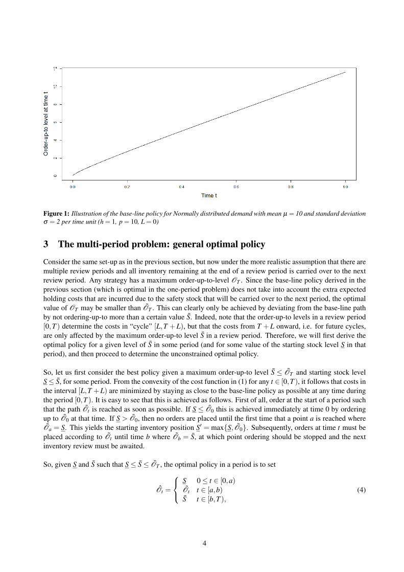
Figure 1: Illustration of the base-line policy for Normally distributed demand with mean µ = 10 and standard deviationσ = 2 per time unit (h = 1, p = 10, L = 0)

3 The multi-period problem: general optimal policy

Consider the same set-up as in the previous section, but now under the more realistic assumption that there aremultiple review periods and all inventory remaining at the end of a review period is carried over to the nextreview period. Any strategy has a maximum order-up-to-level OT . Since the base-line policy derived in theprevious section (which is optimal in the one-period problem) does not take into account the extra expectedholding costs that are incurred due to the safety stock that will be carried over to the next period, the optimalvalue of OT may be smaller than OT . This can clearly only be achieved by deviating from the base-line pathby not ordering-up-to more than a certain value S. Indeed, note that the order-up-to levels in a review period[0,T ) determine the costs in “cycle” [L,T +L), but that the costs from T +L onward, i.e. for future cycles,are only affected by the maximum order-up-to level S in a review period. Therefore, we will first derive theoptimal policy for a given level of S in some period (and for some value of the starting stock level S in thatperiod), and then proceed to determine the unconstrained optimal policy.

So, let us first consider the best policy given a maximum order-up-to level S ≤ OT and starting stock levelS≤ S, for some period. From the convexity of the cost function in (1) for any t ∈ [0,T ), it follows that costs inthe interval [L,T +L) are minimized by staying as close to the base-line policy as possible at any time duringthe period [0,T ). It is easy to see that this is achieved as follows. First of all, order at the start of a period suchthat the path Ot is reached as soon as possible. If S ≤ O0 this is achieved immediately at time 0 by orderingup to O0 at that time. If S > O0, then no orders are placed until the first time that a point a is reached whereOa = S. This yields the starting inventory position S′ = max{S,O0}. Subsequently, orders at time t must beplaced according to Ot until time b where Ob = S, at which point ordering should be stopped and the nextinventory review must be awaited.

So, given S and S such that S≤ S≤ OT , the optimal policy in a period is to set

Ot =

S 0≤ t ∈ [0,a)Ot t ∈ [a,b)S t ∈ [b,T ),

(4)

4

where

a solves Oa = S′, and

b solves Ob = S.

Observe that if S ≤ O0, then a = 0. An illustration of such a policy can be found in Figure 3 of Section 4.It is obvious from the above analysis (and Figure 3) that the optimal level, S, at which to stop ordering isindependent of the starting stock level, S. The latter only affects the time it takes to reach the base-line path.This implies that the optimal policy is stationary in that it applies the same maximum order-up-to level foreach period, independent of the starting stock level.

What remains is to find the optimal value for S. From the above discussion, it follows that the cost of theoptimal policy for a period, given an initial inventory position S, is given by

TC(S, S) = h

a∫0

E(S−Dt+L)+dt +

b∫a

E(Ot −Dt+L)+dt +

T∫b

E(S−Dt+L)+dt

+p

a∫0

E(S−Dt+L)−dt +

b∫a

E(Ot −Dt+L)−dt +

T∫b

E(S−Dt+L)−dt

,This total cost function can be rewritten as

TC(S, S) = h

a∫0

S∫−∞

FDt+L(x)dxdt +b∫

a

Ot∫−∞

FDt+L(x)dxdt +T∫

b

S∫−∞

FDt+L(x)dxdt

+p

a∫0

∞∫S

[1−FDt+L(x)]dxdt +b∫

a

∞∫Ot

[1−FDt+L(x)]dxdt +T∫

b

∞∫S

[1−FDt+L(x)]dxdt

.Using that: (i) the stock at the end of a period is equal to S minus the demand in that period, and (ii) oneorders up to O0 at the start of a period, we get the expected cost per period as

ETC(S) =

∞∫0

TC(S− x, S

)fDT (x)dx

=

S−O0∫0

TC(S− x, S

)fDT (x)dx+P(DT > S− O0)TC(O0, S).

By minimizing this expected cost, the optimal value S can be determined numerically for any demand process.

4 Sensitivity analysis and comparison with pure periodic review

4.1 Numerical examples and sensitivity analysis

The policy derived in the previous section can be applied to any continuous demand process. In this sec-tion, we consider some examples with Normally distributed demand Dr ∼ N(µr,σ2r), zero lead time, and areview period of unit length. For every example, the expected total cost function is approached numericallyby replacing the integrals with variable-dependent bounds by their finite sum equivalents of sufficient length.

Figure 2 shows the expected cycle costs as a function of S for the earlier considered case with µ = 10,σ = 2, h = 1, p = 10, and L = 0. As can be seen, the costs are convex in S and a minimum is achieved

5

Figure 2: Base case example: Derivation of the optimal S for Normally distributed demand with mean µ = 10 andstandard deviation σ = 2 per time unit (p = 10, h = 1, L = 0)

at S ≈ 11.44. Recall that the optimal base-line policy orders up to 12.67. So, the optimal policy is to stopordering in the last phase of the review period, after order-up-to level 11.44 is reached. As this level is stillabove the mean demand of 10 per period, there typically still is (excess) stock left at the start of a period, im-plying an initial phase of the review period without ordering. This leaves a phase in between with continuousordering up to an increasing level. This is illustrated in Figure 3a. In this particular cycle, the observed stocklevel at t = 0 is S = 1.44, which is the expected value of S, given S = 11.44 and µ = 10. This figure shows thetypical three-part structure of the optimal ordering during a review period, with a horizontal start, a slightlydecreasing order speed along the base-line in the middle, and an ordering stop at a level S. Figure 3b showsthe corresponding expected inventory level during the cycle. The expected stock first decreases linearly withslope −µ =−10, after which ordering is started and a safety stock is built up. Finally, orders are halted andthe expected stock level decreases linearly again.

Now that we have seen a full-fledged example of our inventory policy, an interesting question is how itreacts to parameter changes. In Figure 4a and Figure 4b we increase µ (in two steps), ceteris paribus. From(3) we know that an increase in µ leaves the optimal safety stock levels for the base-line policy unchanged.Therefore, the maximum order-up-to level OT increases from 12.7 for µ = 10 to 27.7 for µ = 25 and 52.7for µ = 50. Figures 4a and 4b show that the optimal maximum order-up-to level converges towards OT asµ increases. This is because a higher mean demand rate implies that excess safety stocks, if observed atthe next review, can be depleted at a faster rate and are therefore less costly. Next we analyze the responseof the policy to an increase in demand uncertainty. Specifically, we increase σ to 5. See Figure 4c. Thebase-line policy now orders up to 16.68, whereas the optimal order stop level is S≈ 13.8. Hence, an increasein standard deviation of 150% has led to an increase in the base-line order-up-to level of over 30%, whereasthe optimal order-up-to level increases with approximately 20%. That is, if demand uncertainty increases,then the build-up of safety stock increases in optimum, but the relative deviation from the base-line policyincreases as well.

Instead of altering distribution parameters, we can also study changes in cost parameters. The drawbackof the base-line policy is mainly due to neglection of future holding costs. Let us consider the optimal or-der path if backordering becomes less costly relative to holding costs. In Figure 4d, the backorder cost p isdecreased from 10 to 4. The base-line order level is now decreased to 11.68, whereas the optimal S is now

6

(a) Order path

(b) Expected stock path

Figure 3: Base case example: order path and expected stock path for Normally distributed demand with mean µ =10 and standard deviation σ = 2 per time unit (p = 10, h = 1, L = 0), observed S = 1.44 and corresponding optimalS = 11.44

S≈ 10.45. Hence, compared to the initial case, less safety stock is built up, since a shortage is less expensiveand holding costs have an effect both in the current and in the next period.

7

(a) Mean demand µ per time unit increased to 25 (b) Mean demand µ per time unit increased to 50

(c) Demand variance σ per time unit increased to 5 (d) Backorder cost p per unit per time unit decreased to 4

Figure 4: Sensitivity analysis. Base case: Normally distributed demand with mean µ = 10 and standard deviation σ =2 per time unit (p = 10, h = 1, L = 0)

4.2 Cost savings of continuous over periodic ordering

As discussed in Section 1, most inventory systems in the literature assume either periodic review with pe-riodic ordering, or continuous review with continuous ordering. Under zero ordering costs and with a leadtime equal to 0, the latter will always provide zero cycle costs, as stock can be kept at zero and demandscan be satisfied immediately. So, the cost saving of the optimal continuous ordering policy under periodicreview compared to the optimal periodic ordering policy under periodic review also indicates to what extentcontinuous ordering can compensate for the cost disadvantage of periodic review.

8

We can derive the optimal order-up-to level Sp for periodic ordering by noting that total cycle costs aregiven by

hT∫

0

E(Sp−Dt+L)+dt + p

T∫0

E(Sp−Dt+L)−dt

= hT∫

0

Sp∫−∞

FDt+L(x)dxdt + pT∫

0

∞∫Sp

[1−FDt+L(x)]dxdt,

and so the optimal order-up-to level must satisfy

hT∫

0

FDt+L(Sp)dt = pT∫

0

[1−FDt+L(Sp)]dt.

For the base case, this gives Sp = 9.6 and an expected cycle cost of 5.9. Note that Sp is below the expecteddemand during a review period, despite the 10 to 1 ratio of backorder cost rate vs. holding cost rate. Thereason is that (safety) stocks arrive at the start of a period whereas backorders occur at the end of a period,making it costly to prevent (possible) backorders. Observe that our continuous policy Ot orders more in total,but the spreading of the orders reduces holding costs, such that total costs are only 2.56, which is a reductionby 57%. For σ = 5, the periodic maximum order-up-to level is Sp = 11.7 and the expected cycle cost is 9.3.Figure 5 shows again that Ot orders more in total, but total costs are only 6.45, a reduction by 31%. Hence,a substantial improvement can be made by considering continuous order possibilities, but the improvementdecreases in the variance of the demand distribution. With increasing demand variance, it becomes moredifficult to “predict” demand during a review period and respond with the best continuous ordering plan.

5 Summary & conclusion

In this paper we have presented an optimal inventory policy under periodic review with continuous ordering,for any continuous demand distribution, for any non-negative, deterministic lead time, and for zero fixed or-dering costs. The implied order paths lead to expected inventory paths consisting of two downward slopinglinear parts where no orders are placed, separated by a middle part in which a safety stock is built up at adiminishing rate. An important insight is that typically no order is placed at the start of a period. Instead,excess safety stocks from the previous period are likely to remain. Periodic review ordering policies in theliterature do order at a review and, in fact, typically only at a review. This makes them very ineffective, whichwas confirmed by substantial cost savings of continuous ordering from our numerical examples.

Another important observation from the above described ordering policy is that the build-up of safety stockis not continued until the end of a period. Although the uncertainty surrounding demand since the last reviewdoes continue to increase throughout the period, excess safety stocks increase costs in the first part of the nextreview period. For this reason, no ordering takes place during the last part of a review period.

Given zero ordering costs, the presented policy is applicable and optimal under the quite general conditionsmentioned before. The assumption of continuous demand can be relaxed without severe adaptations, suchthat also discrete alternatives such as the often used Poisson distribution can be studied. Non-deterministiclead times can be approximately dealt with in the same manner as has been suggested for other inventorycontrol systems (see e.g. Axsater (2011)), by increasing the demand variance during the lead time and (partof the) review time. Exact analysis of inventory control models with stochastic lead times is known to be verycomplex, especially if order crossing is allowed.

As follows from our comparisons, in a situation without fixed ordering costs, it can be very lucrative to

9

apply continuous ordering during part of a review period. However, when ordering costs are strictly positive,then such a policy cannot be optimal anymore. An adjusted policy that limits the number of orders placedis needed. This could for instance be achieved by considering more general order level, order-up-to levelpolicies, with both levels changing during a review period. In doing such further research, results on ordersplitting (e.g. by Chiang (2001)) should be taken into account. However, as the term suggests, those modelsstill assume that orders are placed at reviews, and ordering opportunities are also typically predetermined,leaving many opportunities for future research.

Our sensitivity analysis showed that the expected costs incurred by the policy increase when the degree ofrandomness in demand (parametered by σ ) increases. This suggests that further large cost reductions can beaccomplished by integrating (partial) information on demand during the review period into the model in orderto reduce the variance of the remaining, random part. One obvious model is to assume that some but not alldemands are recorded, e.g. customer orders are recorded, but theft, misplacement, etc. are not. Such modelsprovide lower bounds for demand. Similarly, upper bounds can be taken into account. For example, issueslike theft cannot have a larger effect than the current stock at hand. Any method that reduces the uncertaintyin demand will lead to inventory cost reductions. Recall that the ideal situation of complete continuous reviewwith continuous ordering (and under zero lead time) leads to zero costs. Cost improvements of 30 to 60%are achievable by using continuous ordering instead of periodic ordering under periodic review. Timing ofordering is essential in order to realise such a huge cost improvement. This paper shows that it is generallybetter to postpone ordering until some time after the review moment and not order at the review momentitself. Thereby, it makes a fundamental first step in bridging the gap between inefficient periodic review andperiodic ordering policies, and often unrealistic continuous total review and continuous ordering policies.

10

References

Axsater, S. (2006). Inventory control (second ed.). New York: Springer.

Axsater, S. (2011). Inventory control when the lead-time changes. Production and Operations Manage-ment 20(1), 72–80.

Chiang, C. (2001). Order splitting under periodic review inventory systems. International Journal of Produc-tion Economics 70(1), 67 – 76.

Fleisch, E. and C. Tellkamp (2005). Inventory inaccuracy and supply chain performance: a simulation studyof a retail supply chain. International Journal of Production Economics 95(3), 373 – 385.

Flynn, J. and S. Garstka (1990). A dynamic inventory model with periodic auditing. Operations Re-search 38(6), 1089 – 1103.

Goyal, S. K. (1974). Determination of optimum packaging frequency of items jointly replenished. Manage-ment Science 21(4), pp. 436–443.

Nahmias, S. (1982). Perishable inventory theory: A review. Operations Research 30(4), 680 – 708.

Raman, A., N. DeHoratius, and Z. Ton (2001). Execution: The missing link in retail operations. CaliforniaManagement Review 43(3), 136 – 152.

Roushdy, B., N. Sobhy, A. Abdelhamid, and A. Mahmoud (2011). Inventory control for a joint replenishmentproblem with stochastic demand. World Academy of Science, Engineering & Technology, 156 – 160.

Silver, E.A., D.F. Pyke, and R. Peterson (1998). Inventory management and production planning and schedul-ing (third ed.). Hoboken: John Wiley & Sons.

Yano, C. A. and H. L. Lee (1995). Lot sizing with random yields: A review. Operations Research 43(2), 311– 334.

Zhang, R., I. Kaku, and Y. Xiao (2012). Model and heuristic algorithm of the joint replenishment problem withcomplete backordering and correlated demand. International Journal of Production Economics 139(1), 33– 41.

11

1

List of research reports 12001-HRM&OB: Veltrop, D.B., C.L.M. Hermes, T.J.B.M. Postma and J. de Haan, A Tale of Two Factions: Exploring the Relationship between Factional Faultlines and Conflict Management in Pension Fund Boards 12002-EEF: Angelini, V. and J.O. Mierau, Social and Economic Aspects of Childhood Health: Evidence from Western-Europe 12003-Other: Valkenhoef, G.H.M. van, T. Tervonen, E.O. de Brock and H. Hillege, Clinical trials information in drug development and regulation: existing systems and standards 12004-EEF: Toolsema, L.A. and M.A. Allers, Welfare financing: Grant allocation and efficiency 12005-EEF: Boonman, T.M., J.P.A.M. Jacobs and G.H. Kuper, The Global Financial Crisis and currency crises in Latin America 12006-EEF: Kuper, G.H. and E. Sterken, Participation and Performance at the London 2012 Olympics 12007-Other: Zhao, J., G.H.M. van Valkenhoef, E.O. de Brock and H. Hillege, ADDIS: an automated way to do network meta-analysis 12008-GEM: Hoorn, A.A.J. van, Individualism and the cultural roots of management practices 12009-EEF: Dungey, M., J.P.A.M. Jacobs, J. Tian and S. van Norden, On trend-cycle decomposition and data revision 12010-EEF: Jong-A-Pin, R., J-E. Sturm and J. de Haan, Using real-time data to test for political budget cycles 12011-EEF: Samarina, A., Monetary targeting and financial system characteristics: An empirical analysis 12012-EEF: Alessie, R., V. Angelini and P. van Santen, Pension wealth and household savings in Europe: Evidence from SHARELIFE 13001-EEF: Kuper, G.H. and M. Mulder, Cross-border infrastructure constraints, regulatory measures and economic integration of the Dutch – German gas market 13002-EEF: Klein Goldewijk, G.M. and J.P.A.M. Jacobs, The relation between stature and long bone length in the Roman Empire 13003-EEF: Mulder, M. and L. Schoonbeek, Decomposing changes in competition in the Dutch electricity market through the Residual Supply Index 13004-EEF: Kuper, G.H. and M. Mulder, Cross-border constraints, institutional changes and integration of the Dutch – German gas market

2

13005-EEF: Wiese, R., Do political or economic factors drive healthcare financing privatisations? Empirical evidence from OECD countries 13006-EEF: Elhorst, J.P., P. Heijnen, A. Samarina and J.P.A.M. Jacobs, State transfers at different moments in time: A spatial probit approach 13007-EEF: Mierau, J.O., The activity and lethality of militant groups: Ideology, capacity, and environment 13008-EEF: Dijkstra, P.T., M.A. Haan and M. Mulder, The effect of industry structure and yardstick design on strategic behavior with yardstick competition: an experimental study 13009-GEM: Hoorn, A.A.J. van, Values of financial services professionals and the global financial crisis as a crisis of ethics 13010-EEF: Boonman, T.M., Sovereign defaults, business cycles and economic growth in Latin America, 1870-2012 13011-EEF: He, X., J.P.A.M Jacobs, G.H. Kuper and J.E. Ligthart, On the impact of the global financial crisis on the euro area 13012-GEM: Hoorn, A.A.J. van, Generational shifts in managerial values and the coming of a global business culture 13013-EEF: Samarina, A. and J.E. Sturm, Factors leading to inflation targeting – The impact of adoption 13014-EEF: Allers, M.A. and E. Merkus, Soft budget constraint but no moral hazard? The Dutch local government bailout puzzle 13015-GEM: Hoorn, A.A.J. van, Trust and management: Explaining cross-national differences in work autonomy 13016-EEF: Boonman, T.M., J.P.A.M. Jacobs and G.H. Kuper, Sovereign debt crises in Latin America: A market pressure approach 13017-GEM: Oosterhaven, J., M.C. Bouwmeester and M. Nozaki, The impact of production and infrastructure shocks: A non-linear input-output programming approach, tested on an hypothetical economy 13018-EEF: Cavapozzi, D., W. Han and R. Miniaci, Alternative weighting structures for multidimensional poverty assessment 14001-OPERA: Germs, R. and N.D. van Foreest, Optimal control of production-inventory systems with constant and compound poisson demand 14002-EEF: Bao, T. and J. Duffy, Adaptive vs. eductive learning: Theory and evidence 14003-OPERA: Syntetos, A.A. and R.H. Teunter, On the calculation of safety stocks 14004-EEF: Bouwmeester, M.C., J. Oosterhaven and J.M. Rueda-Cantuche, Measuring the EU value added embodied in EU foreign exports by consolidating 27 national supply and use tables for 2000-2007

3

14005-OPERA: Prak, D.R.J., R.H. Teunter and J. Riezebos, Periodic review and continuous ordering

4