arX

iv:1

306.

6756

v2 [

phys

ics.

ins-

det]

4 J

ul 2

013

Performance of the ATLAS Liquid ArgonCalorimeter after Three Years of LHC Operation

and Plans for a Future UpgradeNikiforos Nikiforou, on behalf of the ATLAS Collaboration

Abstract—The ATLAS experiment is designed to study theproton-proton collisions produced at the Large Hadron Collider(LHC) at CERN. Liquid argon sampling calorimeters are used forall electromagnetic calorimetry as well as hadronic calorimetryin the endcaps. After installation in 2004–2006, the calorimeterswere extensively commissioned over the three–year period priorto first collisions in 2009, using cosmic rays and single LHCbeams. Since then, approximately 27 fb−1 of data have beencollected at an unprecedented center of mass energy. Duringall these stages, the calorimeter and its electronics have beenoperating almost optimally, with a performance very close tospecifications. This paper covers all aspects of these first yearsof operation.

The excellent performance achieved is especially presented inthe context of the discovery of the elusive Higgs boson. Thefuture plans to preserve this performance until the end of theLHC program are also presented.

Index Terms—Calorimetry.

I. I NTRODUCTION

T HE ATLAS detector [1] is one of the two large general-purpose experiments designed to study proton-proton

as well as heavy-ion collisions at the CERN Large HadronCollider (LHC). Inside the LHC, bunches of up to1011

protons collide nominally every 25 ns to provide proton-protoncollisions at a design luminosity of1034 cm−2s−1 and a centerof mass energy up to 14 TeV. For its first years of operation, theLHC has been operating at a reduced center of mass energy,namely 7 TeV in 2011 and 8 TeV in 2012, and at an increased50 ns bunch spacing. Already operating close to its designluminosity, the LHC creates an extremely challenging environ-ment for the experiments, by producing multiple interactionsper bunch crossing (pileup), high radiation doses and highparticle multiplicities at unprecedented energies.

The dimensions of the detector (Fig. 1) are 25 m in heightand 44 m in length. The overall weight of the detector isapproximately 7000 tonnes and it is housed in an undergroundexperimental cavern at Point–1 near the CERN main site. Itcovers nearly the entire solid angle around the collision point,and successively consists of an Inner tracking Detector (ID)surrounded by a thin superconducting solenoid, electromag-netic (EM) and hadronic calorimeters, and a muon spectrom-eter incorporating three large toroidal magnet systems.

N. Nikiforou is with the Department of Physics, Columbia University, NewYork, NY 10027 USA (email: nikiforo@cern.ch).

Manuscript received on May 31, 2013.

Fig. 1. Cut-away view of the ATLAS detector [1].

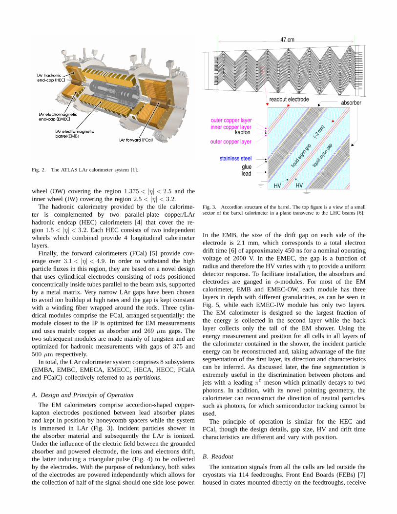
The ATLAS calorimeter system covers the pseudorapid-ity1 range |η| < 4.9 and provides energy measurementsof particles. Sampling calorimeters based on Liquid Argon(LAr) technology are used for the detection of electromagnetic(EM) objects like electrons and photons up to|η| = 3.2, aswell as hadronic objects in the|η| range1.5− 4.9. The LArcalorimeter system (Fig. 2) is the subject of this paper andis described in more detail later. Hadronic calorimetry within|η| < 1.7 is provided by a steel/scintillator-tile calorimeter.

II. T HE ATLAS LA R CALORIMETER SYSTEM

In ATLAS, EM calorimetry is provided by barrel(|η| < 1.475) and endcap (1.375 < |η| < 3.2) accordion ge-ometry lead/LAr sampling calorimeters. An additional thinLAr presampler covering|η| < 1.8 allows corrections forenergy losses in material upstream of the EM calorimeters. Thebarrel electromagnetic (EMB) calorimeter [2] consists of twohalf-barrels housed in the same cryostat. The electromagneticendcap calorimeter (EMEC) [3] comprises two wheels, oneon each side of the EM barrel. The wheels are containedin independent endcap cryostats together with the hadronicendcap and forward calorimeters described later. The wheelsthemselves consist of two co-axial wheels, with the outer

1ATLAS uses a right-handed coordinate system with its originat thenominal interaction point (IP) in the center of the detectorand thez-axisalong the beam pipe. Thex-axis points from the IP to the center of the LHCring, and they-axis points upward. Cylindrical coordinates(r, φ) are used inthe transverse plane,φ being the azimuthal angle around the beam pipe. Thepseudorapidity is defined in terms of the polar angleθ asη = − ln tan(θ/2).In ATLAS, the so-called “side-A” refers to positivez-values while “side-C”refers to the negative side.

(EMB)

Fig. 2. The ATLAS LAr calorimeter system [1].

wheel (OW) covering the region1.375 < |η| < 2.5 and theinner wheel (IW) covering the region2.5 < |η| < 3.2.

The hadronic calorimetry provided by the tile calorime-ter is complemented by two parallel-plate copper/LArhadronic endcap (HEC) calorimeters [4] that cover the re-gion 1.5 < |η| < 3.2. Each HEC consists of two independentwheels which combined provide 4 longitudinal calorimeterlayers.

Finally, the forward calorimeters (FCal) [5] provide cov-erage over3.1 < |η| < 4.9. In order to withstand the highparticle fluxes in this region, they are based on a novel designthat uses cylindrical electrodes consisting of rods positionedconcentrically inside tubes parallel to the beam axis, supportedby a metal matrix. Very narrow LAr gaps have been chosento avoid ion buildup at high rates and the gap is kept constantwith a winding fiber wrapped around the rods. Three cylin-drical modules comprise the FCal, arranged sequentially; themodule closest to the IP is optimized for EM measurementsand uses mainly copper as absorber and269 µm gaps. Thetwo subsequent modules are made mainly of tungsten and areoptimized for hadronic measurements with gaps of375 and500 µm respectively.

In total, the LAr calorimeter system comprises 8 subsystems(EMBA, EMBC, EMECA, EMECC, HECA, HECC, FCalAand FCalC) collectively referred to aspartitions.

A. Design and Principle of Operation

The EM calorimeters comprise accordion-shaped copper-kapton electrodes positioned between lead absorber platesand kept in position by honeycomb spacers while the systemis immersed in LAr (Fig. 3). Incident particles shower inthe absorber material and subsequently the LAr is ionized.Under the influence of the electric field between the groundedabsorber and powered electrode, the ions and electrons drift,the latter inducing a triangular pulse (Fig. 4) to be collectedby the electrodes. With the purpose of redundancy, both sidesof the electrodes are powered independently which allows forthe collection of half of the signal should one side lose power.

47 cm

readout electrodeabsorber

leadglue

kapton

outer copper layer

outer copper layer

inner copper layer

stainless steel

HVHV

liqui

d ar

gon

gap

liqui

d ar

gon

gap

(~2

mm

)

Fig. 3. Accordion structure of the barrel. The top figure is a view of a smallsector of the barrel calorimeter in a plane transverse to theLHC beams [6].

In the EMB, the size of the drift gap on each side of theelectrode is 2.1 mm, which corresponds to a total electrondrift time [6] of approximately 450 ns for a nominal operatingvoltage of 2000 V. In the EMEC, the gap is a function ofradius and therefore the HV varies withη to provide a uniformdetector response. To facilitate installation, the absorbers andelectrodes are ganged inφ-modules. For most of the EMcalorimeter, EMB and EMEC-OW, each module has threelayers in depth with different granularities, as can be seeninFig. 5, while each EMEC-IW module has only two layers.The EM calorimeter is designed so the largest fraction ofthe energy is collected in the second layer while the backlayer collects only the tail of the EM shower. Using theenergy measurement and position for all cells in all layers ofthe calorimeter contained in the shower, the incident particleenergy can be reconstructed and, taking advantage of the finesegmentation of the first layer, its direction and characteristicscan be inferred. As discussed later, the fine segmentation isextremely useful in the discrimination between photons andjets with a leadingπ0 meson which primarily decays to twophotons. In addition, with its novel pointing geometry, thecalorimeter can reconstruct the direction of neutral particles,such as photons, for which semiconductor tracking cannot beused.

The principle of operation is similar for the HEC andFCal, though the design details, gap size, HV and drift timecharacteristics are different and vary with position.

B. Readout

The ionization signals from all the cells are led outside thecryostats via 114 feedtroughs. Front End Boards (FEBs) [7]housed in crates mounted directly on the feedtroughs, receive

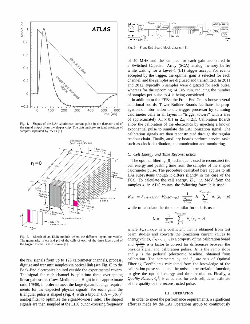
Fig. 4. Shapes of the LAr calorimeter current pulse in the detector and ofthe signal output from the shaper chip. The dots indicate an ideal position ofsamples separated by 25 ns [1].

∆ϕ = 0.0245

∆η = 0.025

37.5mm/8 = 4.69 mmm∆η = 0.0031

∆ϕ=0.0245x436.8mmx

Trigger Tower

∆ϕ = 0.0982

∆η = 0.1

16X0

4.3X0

2X0

1500

mm

470

mm

η

ϕ

η=0

Strip cel l s in L ayer 1

Square cel l s in

L ayer 2

1.7X0

Cells in Layer 3

∆ϕ×∆η = 0.0245×0.05

Cells in PS

∆η×∆ϕ = 0.025×0.1

TriggerTower

=147.3mm4

Fig. 5. Sketch of an EMB module where the different layers arevisible.The granularity in eta and phi of the cells of each of the threelayers and ofthe trigger towers is also shown [1].

the raw signals from up to 128 calorimeter channels, process,digitize and transmit samples via optical link (see Fig. 6) to theBack-End electronics housed outside the experimental cavern.The signal for each channel is split into three overlappinglinear gain scales (Low, Medium and High) in the approximateratio 1/9/80, in order to meet the large dynamic range require-ments for the expected physics signals. For each gain, thetriangular pulse is shaped (Fig. 4) with a bipolarCR−(RC)2

analog filter to optimize the signal-to-noise ratio. The shapedsignals are then sampled at the LHC bunch-crossing frequency

Fig. 6. Front End Board block diagram [1].

of 40 MHz and the samples for each gain are stored ina Switched Capacitor Array (SCA) analog memory bufferwhile waiting for a Level–1 (L1) trigger accept. For eventsaccepted by the trigger, the optimal gain is selected for eachchannel, and the samples are digitized and transmitted. In 2011and 2012, typically 5 samples were digitized for each pulse,whereas for the upcoming 14 TeV run, reducing the numberof samples per pulse to 4 is being considered.

In addition to the FEBs, the Front End Crates house severaladditional boards. Tower Builder Boards facilitate the prop-agation of information to the trigger processor by summingcalorimeter cells in all layers in “trigger towers” with a sizeof approximately0.1 × 0.1 in ∆η ×∆φ. Calibration Boardsallow the calibration of the electronics by injecting a knownexponential pulse to simulate the LAr ionization signal. Thecalibration signals are then reconstructed through the regularreadout chain. Finally, auxiliary boards perform service taskssuch as clock distribution, communication and monitoring.

C. Cell Energy and Time Reconstruction

The optimal filtering [8] technique is used to reconstruct thecell energy and peaking time from the samples of the shapedcalorimeter pulse. The procedure described here applies toallLAr subsystems though it differs slightly in the case of theFCal. To calculate the cell energy,Ecell in MeV, from thesamplessj in ADC counts, the following formula is used:

Ecell = FµA→MeV ·FDAC→µA · 1Mphys

Mcali

·RNsamples∑

j=1

aj (sj − p)

while to calculate the time a similar formula is used:

tcell =1

Ecell

Nsamples∑

j=1

bj (sj − p)

whereFµA→MeV is a coefficient that is obtained from testbeam studies and converts the ionization current values toenergy values,FDAC→µA is a property of the calibration boardand Mphys

Mcaliis a factor to correct for differences between the

physics signal and calibration pulses.R is the ramp slopeand p is the pedestal (electronic baseline) obtained fromcalibration. The parametersaj and bj are sets of OptimalFiltering Coefficients calculated from the knowledge of thecalibration pulse shape and the noise autocorrelation function,to give the optimal energy and time resolution. Finally, aQuality Factor, Q2, is calculated for each cell, as an estimateof the quality of the reconstructed pulse.

III. OPERATION

In order to meet the performance requirements, a significanteffort is made by the LAr Operations group to continuously

monitor the detector status and performance and take cor-rective actions if needed. This task is supported by variousmonitoring systems conceived and installed for this purpose.A Detector Control System (DCS) has been developed in theATLAS-wide DCS framework to provide control, monitoringand human interface with the hardware, based on the commer-cial SCADA software PVSS-II (now named SIMATIC WinCCOpen Architecture) [9].

A. Cryogenic System Stability

The cryogenic system aims to provide stable LAr condi-tions. The temperature sensitivity of the LAr calorimeter hasbeen determined to follow a linear relationship with a 2%decrease of the measured signal per kelvin. This includes thecontribution from LAr density variations with temperatureaswell as drift velocity variations, contributing to changesof-0.45%/K and -1.55%/K respectively. In order to meet thedesign energy resolution, a 100 mK temperature stability anduniformity is required.

A temperature monitoring system is in place to monitorand log the conditions so as to be able to correct for anytemperature variations and non-uniformities. The temperaturemonitoring system comprises more than 400 calibrated preci-sion temperature probes (PT100 platinum resistors) distributedthroughout the three cryostats and immersed in the LAr. Mea-surements are taken every minute and a conditions database isupdated if there is a change from the previous measurement.

Periodic studies are performed to monitor the stability ofthe cryogenic system during data taking. Temperature data arecollected over long periods of time without interventions onthe cryogenic system and low voltage power supply and forconstant general conditions, such as the magnetic field. Fig. 7shows the temperature uniformity of the LAr barrel calorime-ter, demonstrating an overall barrel temperature uniformity of59 mK for data collected over a period of 10 days. Similaror better results are obtained in the endcaps, satisfying thedesign requirements. Finally, Fig. 8 shows the distribution ofthe RMS of the temperature measurements for each of thetemperature probes in the LAr calorimeter cryostats, over thesame period. The average RMS of 1.5 mK demonstrates thereliability of the temperature control and monitoring system.

An additional source of non-uniformity in the cryogenicsystem arises from the presence of impurities in the LAr.Ionization signal electrons can attach to electronegativeimpu-rities, such asO2, which would lead to the degradation of thesignal measurement. A limit of 1000 ppb oxygen impuritiesor equivalent has been set for the efficient operation of thecalorimeter.

The stability of the LAr purity is monitored in 10 to 15minute intervals by a system of 30 purity monitors [11] in-stalled throughout the cryostats. Each purity monitor measuresthe deposition of known charges from two contained monoen-ergetic radioactive sources (207Bi and 241Am) in ionizationchambers. The monitors were shown to have a systematicuncertainty of 19% and a statistical uncertainty for a singlemeasurement of∼ 5 ppb. Fig. 9 shows the impurity levels overthe course of two years between July 2007 and July 2009 for

Temperature [K]

88.3 88.4 88.5 88.6 88.7 88.8 88.9

Num

ber

of p

robe

s

0

5

10

15

20

25

RMS : 59 mK

161 probes

ATLAS

EM BARREL

Fig. 7. Distribution of the average temperature measured over ten days fortemperature probes within the EM Barrel cryostat [10].

Temperature RMS [mK]

0 0.5 1 1.5 2 2.5 3 3.5 4 4.5 5

Num

ber

of p

robe

s

0

10

20

30

40

50

60

Average dispersion : 1.5 mK

429 probes

ATLAS

Fig. 8. Distribution of the RMS of the temperature measurements, over tendays, for each of the temperature probes within all three of the LAr calorimetercryostats [10].

HECA. The overall levels of impurities have been measuredto be approximately200 ppb and140 ppb in the barrel andendcap cryostats respectively, well below the operationallimit.Finally, the levels have been shown to be stable except in thecase of side C of the endcap where a small degradation ofapproximately5 ppb per year is observed.

B. High Voltage Operation

The high voltage (HV) system provides the electric fieldso that the ionization signal propagates to the measurementelectrodes for readout. The HV values are monitored inreal time via the DCS system and stored in a conditionsdatabase. Suitable corrections are applied during the energyreconstruction for any deviations from the nominal values.

During data taking, some HV hardware modules may trip,which leads to loss of power to one side of an electrode,thereby inhibiting the signal measurement. Procedures havebeen established for the manual recovery of tripped HVlines on a case-by-case basis. In addition, an autorecovery

Date DD/MM/YYYY02/07/2007 01/01/2008 01/07/2008 31/12/2008 02/07/2009

Imp

uri

ty [

pp

b]

100

120

140

160

180

200

Purity HEC1 A APurity HEC1 A BPurity HEC1 A CPurity HEC2 A APurity HEC2 A BPurity HEC2 A C

1000 ppb≈Require purity better

Purity HEC1/2 Side A

Fig. 9. Impurity levels inO2 equivalents for HECA. Each point shows themean of the purity values measured over a single day and excludes extremeor unreasonable values that can be attributed to instrumental effects [10].

HV correction factor1 1.2 1.4 1.6 1.8 2

nu

mb

er o

f re

ado

ut

chan

nel

s

1

10

210

310

410

510

30. Aug. 10

LAr correction factors for reduced High Voltage

Fig. 10. Distribution of cell energy correction factors applied for channelsserviced by at least one HV line operated at reduced voltage [12].

system has been implemented for modules that are not trippingsystematically. Owing to the frequent measurement of the HVvalues, data recorded during the ramp-up of tripped lines canbe corrected and used in analysis. Specialized studies wereperformed to verify that data collected during HV recoverycan safely be used in analysis. During the trip itself, the rapidvariation of the voltage makes the proper correction of thesignal impractical, leading to a small loss of data. In orderto limit the number of trips and minimize this inefficiency,problematic lines that trip frequently are set to lower operatingHV values and a correction is applied for the energy of theaffected cells. A typical distribution of correction factors isshown in Fig. 10. Finally, more robust HV modules havebeen deployed that allow the module to run in current controlmode instead of tripping, which prevents the voltage drop.All the above improvements result in the minimization of datarejection due to HV trips in 2012 which was limited to 0.46%.

C. Electronics Calibration and Stability

Calibration campaigns are performed regularly and involvespecial runs in the absence of LHC beams to measure theresponse of the FEB electronics in situ for each of thethree gains. An infrastructure has been deployed to facilitatethe retrieval and processing of those runs, the extraction ofcalibration constants and their propagation to a conditionsdatabase.

Daily pedestal and noise levels for each channel are de-termined by “Pedestal” runs where the channel is triggeredwithout signal injection. The pedestal is computed for eachchannel from the average over the triggers and the number ofsamples.

In order to determine the gain for each channel, “Ramp”runs are also taken on a daily basis. In these runs, eachchannel is pulsed several times with a set of predeterminedcalibration board DAC values, corresponding to input currents.For each DAC value, the resulting pulses are reconstructedand an average pulse shape is computed from which the peakADC value is measured. Thus, the relationship between theDAC and ADC values is obtained for each channel and, byfitting it with a first order polynomial, the ramp slopeR iscalculated.

To demonstrate the excellent stability of the LAr electronics,Fig. 11 shows example stability plots for the pedestal and gainvalues with respect to time in 2012, for FEBs in the LAr EMcalorimeters (EMB and EMEC) in High gain. For each FEB,the pedestal and gain average over all channels serviced by thatboard is calculated and plotted as a function of time. Comparedto a reference value, the pedestal difference distributionhas anRMS of 0.030 ADC counts, while the relative gain differencedistribution has an RMS of 0.343 per mil. The stability issimilar for the other LAr calorimeters (HEC and FCal) andin the other gains, with a pedestal difference RMS rangingfrom 0.022 to 0.029 ADC counts. Finally, the relative gaindifference is distributed with an RMS between 0.316 and 0.343per mil for the EM calorimeters, 0.657–0.814 per mil for theHEC and 0.046–0.086 per mil for the FCal.

Finally, “Delay” runs are taken weekly or as often as itis needed to reconstruct the pulse shape itself in detail. Inthis mode, for each calibration pulse, the channel is triggeredseveral times with incremental delays of 1.04 ns. On eachtrigger, 32 samples are acquired at 40 MHz and the entirepulse is therefore effectively sampled at 1.04 ns, allowingreconstruction of the pulse shape with high precision. Eachchannel is further pulsed several times and the procedure isrepeated to calculate an average pulse shape. The shape is usedto extract the Optimal Filtering Coefficients that describetheshape and are used in the energy and time reconstruction frompulse samples as well as the calculation of the quality of thereconstructed pulse.

The values of the calibration constants are monitored forsignificant variations and are updated in the database typicallyonce a month, or whenever there is a change in the systemconditions.

Date in 201220.04 20.05 19.06 19.07 18.08 17.09 17.10 16.11

PE

DE

STA

L (A

DC

cou

nt)

∆

-0.2

-0.1

0

0.1

0.2

0

20

40

60

80

100

120

ATLAS Preliminary

LAr EM High Gain1376 FEBs

Nb FEBs

0 1000 2000

-0.2

-0.15

-0.1

-0.05

0

0.05

0.1

0.15

0.2 Overflow=3Underflow=8

RMS=0.030 ADC

Date in 201220.04 20.05 19.06 19.07 18.08 17.09 17.10 16.11

GA

IN/G

AIN

(pe

r m

il)∆

-4

-2

0

2

4

0

50

100

150

200

250

300

350

400

ATLAS Preliminary

LAr EM High Gain1376 FEBs

Nb FEBs

0 5000-4

-3

-2

-1

0

1

2

3

4

5

Overflow=4Underflow=2

RMS=0.343 per mil

Fig. 11. Pedestal stability (top) and ramp stability (bottom) with respect totime in 2012 for the LAr EM calorimeters in High gain [10].

D. Timing

A precise timing measurement of calorimeter signals isparticularly useful in the operation of the detector as wellas physics analyses. Knowledge of time with a precisionsmall compared to 25 ns (the nominal LHC bunch interval)is required to differentiate between energy deposits origi-nating from collisions in the triggered bunch crossing asopposed to signals from neighboring bunch crossings. Thelatter phenomenon is known as “out-of-time pileup”. Further,excellent timing can be used to reject other sources of beaminduced background such as satellite collisions and beamhalo [13]. In addition, it provides a means to veto events withenergy deposited by cosmic ray interactions overlapping withthe triggered event. Finally, the timing can be employed insearches for new physics involving long-lived neutral particlesdecaying to photons [14], electrons or jets.

The timing measurement is performed with respect to theLHC clock phase delivered from a central system to ATLASby means of an optical fiber. The clock phase can drift, forexample, due to variations of the fiber length with temperature,and this can be detected by comparing with the actual buncharrival times in ATLAS. The average time is monitored andis corrected for any global variations such as the LHC clockdrift. In 2012, the capability to automatically compensateforany clock drift with a precision of a few tens of ps was

Run number

2010

06

2026

60

2065

64

2088

11

2095

50

2098

99

2118

67

2126

19

2130

39

> [n

s]F

EB

<t

-2

-1.5

-1

-0.5

0

0.5

1

1.5

2

EMB

EMEC

HEC

FCAL

FEB Correction

FCAL HV modulesreplacement

LHC clock driftcompensation off

LHC clock driftautomaticallycompensated

March - mid May-1~1.6 fb

mid May - October-1~14 fb

ATLAS Preliminary

Fig. 12. Mean FEB time synchronization for each LAr partition [12].

> [ns]FEB<t

-4 -2 0 2 4

Num

ber

of F

EB

s pe

r 0.

25 n

s

10

= 8 TeV collisionss FCAL

May 2012

= 0.09 nsσ

ATLAS Preliminary

Fig. 13. Average time per Front End Board in the FCal with 8 TeVcollisiondata on May 2012 [12].

implemented during the June technical stop and performedvery well as shown in Fig. 12.

The calorimeter is timed in with collision data with anonline precision of approximately 1 ns. As shown in Fig. 13,the calorimeter is properly aligned and uniform in time, witha typical spread of the average FEB time between 0.09 ns and0.17 ns, depending on the partition.

To improve the timing performance of the EM calorimetersfurther, a number of effects were studied and corrected forwith good quality W → eν events. Additional calibrationconstants are computed as a function of the data taking period,FEB, channel within the FEB, cell energy and primary vertexposition. After all constants are applied, a timing resolution of≈ 290 ps is achieved for large energy depositions in the EMB,as shown in Fig. 14. By comparing the corrected time of thetwo electrons inZ → ee events, this resolution is understoodto include a correlated contribution of≈ 220 ps, expected to be

Cell Energy [GeV]5 10 15 20 25 30 35 40

Tim

e R

esol

utio

n [n

s]

0.25

0.30

0.35

0.40

0.45

0.50

ATLASData 2011

-1Ldt= 4.8 fb∫=7 TeV, s

Data 2011

Fit

Fig. 14. Single cell time resolution energy dependence, forcells reconstructedin High gain, in the Middle layer of the LAr EM Barrel Calorimeter(|η| < 1.4). A fit with the expected energy dependence, comprising a so-called “noise term” and a “constant term”, added in quadrature, is shownsuperimposed [14].

dominated by the spread of the proton bunches along the LHCbeamline, and an uncorrelated contribution of≈ 190 ps. Thelatter component includes the intrinsic timing resolutionof theLAr EMB and its readout, as well as residual non-uniformitiesand imperfections in the calibration procedure.

IV. DATA QUALITY MONITORING

A complex monitoring procedure was designed to track andquickly identify all potential problems affecting the detector,including the situations described in previous sections. TheData Quality Monitoring effort involves low level hardwaremonitoring via the DCS system as well as checks in everystage of the data acquisition and processing chain. Severalalgorithms assist trained personnel during the data taking(online monitoring) in detecting issues that could compromisedata quality, so corrective actions can be taken. Offline, moredetailed tests are performed using a subset of the recordeddata which are expeditiously reconstructed to pinpoint blocksof data with suspected quality issues, ordefects, before theprocessing of the bulk of the data is launched 48 hours later.The results of the tests are organized through a dedicated webinfrastructure and trained experts decide on the defect type,localization, severity and length in time, with the ultimategoal of optimal detector efficiency. During this process, thedetector conditions during the data taking, stored via DCSare also taken into account (for example HV values andstatus). The proposed actions are propagated as needed to therelevant conditions databases via automated procedures. Afterthe bulk processing is completed, typically several days later,a final data quality assessment is performed to verify that theproblems identified in the previous steps have been handled

x[m]

-2.5 -2 -1.5 -1 -0.5 0 0.5 1 1.5 2 2.5

y[m

]

-2.5

-2

-1.5

-1

-0.5

0

0.5

1

1.5

2

2.5

Ene

rgy[

MeV

]

210

310

410

510

610ATLAS Preliminary

Fig. 15. Example of a single event affected by a noise burst recorded inempty LHC bunches in EMECA [12].

properly. If needed, the databases are further updated to flagthe remaining issues and, if possible, to allow the recoveryofdata in future reprocessing.

A significant source of possible LAr inefficiency with aninteresting pathology is the presence of bursts of large scalecoherent noise, ornoise bursts, mainly located in the endcaps.This phenomenon manifests itself only in the presence ofcollisions and was found to scale with instantaneous lumi-nosity. The effect is very short in time, lasting usually lessthan∼ 5 µs, and during that time a significant percentage ofchannels exhibit signal readings which are significantly abovethe typical electronic noise levels. An example of such anevent is shown in Fig. 15.

A useful variable for the description of noise burst eventsis Y3σ which represents the percentage of channels with asignal greater than three times the electronic noise measuredduring the LHC beam crossings without collisions (emptybunches). Hard noise burst events with largeY3σ are efficientlyidentified and flagged using the quality factors of the pulsemeasurements. However it was found that softer noise bursts,usually peripheral to a hard event and characterized by aY3σof the order 2-3%, are not efficiently flagged. Taking advantageof the short nature of the phenomenon, atime window vetoprocedure was established to identify these occurrences andreject neighboring events within a conservative time windowaround the identified noise burst. The window length was 1 sfor 2011 and 250 ms for the 2012 data taking period. Theefficiency of this method in rejecting large scale coherent noiseevents in empty bunches is demonstrated by Fig. 16.

The procedures described above were established and im-proved over the last few years of ATLAS operation andresulted in a continuous improvement in data quality and nearoptimal LAr efficiency. For 2012, the LAr inefficiency waslimited to 0.88% of which 0.46% is due to HV trips while0.2% is attributed to noise bursts.

[%]σ3Y

0 1 2 3 4 5 6 7 8 9 10

Eve

nts/

0.1%

1

10

210

310

410

510

610

)-1Data acquired in empty bunches with LHC in collision mode (135 hours/1.7 fb

8033 events above 10% (60/h)14664 events above 1% (109/h)

No veto -

0 events above 10%1644 events above 1% (12/h)

Standard flag -

0 events above 10%417 events above 1% (3/h)

t = 250 ms) - δVeto (

ATLAS Preliminary

Fig. 16. Distribution of the percentage of noisy channels inthe EM endcap,measured during empty bunches in LHC collision mode. The black pointsshow the percentage without any corrective action. The red points representthe data after rejection of events identified by means of the quality factor onlywhile the green points show the effect of the time veto procedure [12].

V. PHYSICS PERFORMANCE

While the low-level detector hardware and Data Qualitymonitoring are paramount to the successful running of theexperiment, the ultimate goal is to reconstruct interestingphysics events with efficiency, reliability and precision.It isthe responsibility of the LAr calorimeter system to provideexcellent measurements of physics objects, such as electrons,photons and jets, and contribute to the calculation of the eventmissing energy with high resolution. Tests at the physics levelare performed continuously during the data taking periodsusing benchmark physics processes to gauge the object re-construction stability and precision.

A. Energy Scale, Resolution and Stability

A detailed study was performed [15] to determine theelectron performance of the ATLAS detector using the decaysof the Z, W andJ/ψ particles. The studies demonstrate thelevel of energy scale, resolution and uniformity of the LArsystem as well the excellent overall performance of the ATLASdetector.

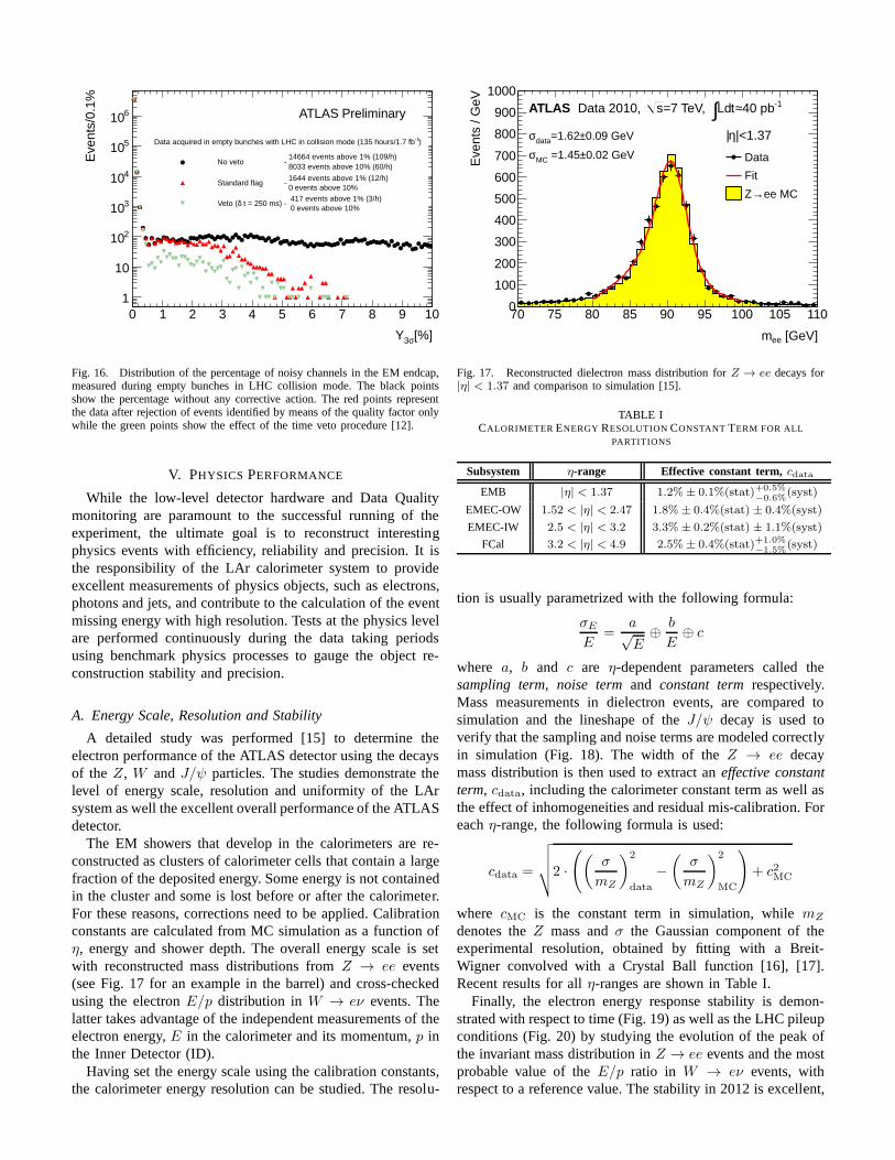
The EM showers that develop in the calorimeters are re-constructed as clusters of calorimeter cells that contain alargefraction of the deposited energy. Some energy is not containedin the cluster and some is lost before or after the calorimeter.For these reasons, corrections need to be applied. Calibrationconstants are calculated from MC simulation as a function ofη, energy and shower depth. The overall energy scale is setwith reconstructed mass distributions fromZ → ee events(see Fig. 17 for an example in the barrel) and cross-checkedusing the electronE/p distribution inW → eν events. Thelatter takes advantage of the independent measurements of theelectron energy,E in the calorimeter and its momentum,p inthe Inner Detector (ID).

Having set the energy scale using the calibration constants,the calorimeter energy resolution can be studied. The resolu-

[GeV]eem

70 75 80 85 90 95 100 105 110

Eve

nts

/ GeV

0

100

200

300

400

500

600

700

800

900

1000

Data

Fit

MCee→Z

|<1.37η|0.09 GeV±=1.62dataσ

0.02 GeV± =1.45MCσ

ATLAS =7 TeV,sData 2010, ∫ -140 pb≈tdL

Fig. 17. Reconstructed dielectron mass distribution forZ → ee decays for|η| < 1.37 and comparison to simulation [15].

TABLE ICALORIMETER ENERGY RESOLUTIONCONSTANT TERM FOR ALL

PARTITIONS

Subsystem η-range Effective constant term, cdata

EMB |η| < 1.37 1.2%± 0.1%(stat)+0.5%

−0.6%(syst)

EMEC-OW 1.52 < |η| < 2.47 1.8%± 0.4%(stat) ± 0.4%(syst)

EMEC-IW 2.5 < |η| < 3.2 3.3%± 0.2%(stat) ± 1.1%(syst)

FCal 3.2 < |η| < 4.9 2.5%± 0.4%(stat)+1.0%

−1.5%(syst)

tion is usually parametrized with the following formula:

σEE

=a√E

⊕ b

E⊕ c

where a, b and c are η-dependent parameters called thesampling term, noise termand constant termrespectively.Mass measurements in dielectron events, are compared tosimulation and the lineshape of theJ/ψ decay is used toverify that the sampling and noise terms are modeled correctlyin simulation (Fig. 18). The width of theZ → ee decaymass distribution is then used to extract aneffective constantterm, cdata, including the calorimeter constant term as well asthe effect of inhomogeneities and residual mis-calibration. Foreachη-range, the following formula is used:

cdata =

√

√

√

√2 ·(

(

σ

mZ

)2

data

−(

σ

mZ

)2

MC

)

+ c2MC

where cMC is the constant term in simulation, whilemZ

denotes theZ mass andσ the Gaussian component of theexperimental resolution, obtained by fitting with a Breit-Wigner convolved with a Crystal Ball function [16], [17].Recent results for allη-ranges are shown in Table I.

Finally, the electron energy response stability is demon-strated with respect to time (Fig. 19) as well as the LHC pileupconditions (Fig. 20) by studying the evolution of the peak ofthe invariant mass distribution inZ → ee events and the mostprobable value of theE/p ratio in W → eν events, withrespect to a reference value. The stability in 2012 is excellent,

[GeV]eem1 1.5 2 2.5 3 3.5 4

Eve

nts

/ 0.0

75 G

eV

0

200

400

600

800

1000

1200

1400

1600

1800

2000

DataFit

MCee→ψJ/Background from fit

2 MeV± = 3080data

µ1 MeV± = 3083

MCµ

2 MeV± = 132dataσ1 MeV± = 134MCσ

ATLAS =7 TeV,sData 2010, ∫ -140 pb≈tdL

Fig. 18. Reconstructed dielectron mass distribution forJ/ψ → ee decaysand comparison to simulation [15].

Date (Day/Month)

03⁄26 04⁄25 05⁄25 06⁄24 07⁄24 08⁄23 09⁄22

Rel

ativ

e en

ergy

sca

le

0.995

0.996

0.997

0.998

0.999

1

1.001

1.002

1.003

1.004

1.005

RMS: 0.023%RMS: 0.033%

E/pνe→ Wee inv. mass→ Z

ATLAS Preliminary

-1 13.0 fb= tdL∫=8 TeV, sData 2012,

Fig. 19. Electron energy response stability with time in 2012 data [18].

Fig. 20. Electron energy response stability with pileup (average number ofinteractions per bunch crossing) in 2012 data [19].

better than0.03% which is expected for a LAr calorimeterwith stable temperature and purity conditions.

Number of reconstructed primary vertices

0 2 4 6 8 10 12 14 16 18 20

Ele

ctro

n id

entif

icat

ion

effic

ienc

y [%

]

60

65

70

75

80

85

90

95

100

105ATLAS Preliminary -1

4.7 fb≈ Ldt ∫Data 2011

Loose++

2012 selection

2011 selection

Medium++

2012 selection

2011 selection

Tight++

2012 selection

2011 selection

Fig. 21. Dependence of electron identification efficiency onpileup, measuredusingZ → ee, J/ψ → ee andW → eν events [21].

B. Identification Efficiency

In addition to having good resolution and uniformity, thecalorimeter is required to have excellent electron/photoniden-tification efficiency and a high jet rejection rate over a broadenergy range. The fine segmentation of the LAr calorimetermakes this possible by providing valuable information forthe shape and other characteristics of the EM showers. Inaddition, photons which leave no tracks in the ID can beefficiently detected and their direction measured using thesame feature. More specifically, the photon flight directioncan be reconstructed by measuring precisely the position ofthe cluster barycenters in the first and second LAr calorimeterlayers in depth.

In ATLAS, electron identification [20] is performed witha cut-based method combining information from the showershape characteristics in the calorimeter with the informationfrom the ID where available. Three reference sets of cutshave been defined with increasing background rejection power:loose, mediumand tight with an expected jet rejection ofapproximately 500, 5000 and 50000, respectively, based onMC simulation. The values of the cuts are optimized accordingto the beam conditions, leading to an improved set of cuts for2012 which performs better in high pileup conditions whilemaintaining similar jet rejection power. As can be seen in Fig.21, an identification efficiency exceeding 95%, 88% and 79%is achieved in 2012 forloose, mediumand tight respectively,for up to 20 reconstructed primary vertices per event.

Photon reconstruction [23] is similar to electrons albeitmore involved due to the fact that photons can be eitherunconverted or converted. The latter are characterized by thepresence of at least one track in the ID that matches theEM cluster in the calorimeter, resulting in an ambiguity inthe distinction between converted photons and electrons. Inaddition, unconverted photons can also be reconstructed aselectrons if their EM clusters are erroneously associated withtracks that typically have low momentum. For this reason, aprocedure has been established to recover photon candidatesfrom a collection of electron candidates, based on combinedinformation from the ID and the calorimeter (number andmomentum of matched tracks, number and position of hitsin the ID, E/p ratio). To provide a pure photon sample and

γ IDε

0.45

0.5

0.55

0.6

0.65

0.7

0.75

0.8

0.85

0.9

0.95

1

ATLAS Preliminary

= 8 TeVs , -1

Ldt = 20.7 fb∫| < 0.6η, |γUnconverted

data 2012γ ll→Z

simulationγ ll→Z

[GeV]γTE

10 15 20 25 30 35 40 45 50 55 60 65 70 75 80

Dat

aγ IDε-

MC

γ IDε -0.1-0.05

00.05

0.1

γ IDε

0.45

0.5

0.55

0.6

0.65

0.7

0.75

0.8

0.85

0.9

0.95

1

ATLAS Preliminary

= 8 TeVs , -1

Ldt = 20.7 fb∫| < 0.6η, |γConverted

data 2012γ ll→Z

simulationγ ll→Z

[GeV]γTE

10 15 20 25 30 35 40 45 50 55 60 65 70 75 80

Dat

aγ IDε-

MC

γ IDε -0.1-0.05

00.05

0.1

Fig. 22. Photon identification efficiency for unconverted (top) and converted(bottom) photon candidates obtained inZ → ℓℓγ events, for|η| < 0.6.Similar performance is observed in otherη ranges [22].

study the photon identification efficiency, the radiativeZ decayZ → ℓℓγ is exploited [22], where the leptonℓ, can be anelectron or a muon. In these studies, no requirements on thephoton shower shape are applied, to avoid any bias. As shownin Fig. 22, the efficiency is very high for both convertedand unconverted candidates, and agrees with the expectedperformance from MC simulation.

The fine granularity of the calorimeter is a significant assetallowing the separation of photons from jets. As can be seenin Fig. 23, the shower shape for a photon is expected tohave a narrower profile compared to the shower shape fora jet. Especially in the presence of aπ0 meson, a distinctiveenergy deposition with two energy maxima is expected in thefirst layer of the LAr calorimeter (strips). To efficiently rejectbackground in analyses using photons, photon identificationis performed, similarly to electrons, using the characteristicsof their shower shape. Two reference sets of cuts,looseandtight, are defined. The former set of cuts has a very highefficiency with a modest jet rejection power, while the latterhas a rejection power of approximately 5000 while keeping a

Fig. 23. Shower shapes for a photon candidate (left) and a candidate for ajet with a leadingπ0 (right), in data recorded in proton-proton collisions [25].

relatively high efficiency, approximately 85% for photons withtransverse energyET > 40 GeV [24].

C. The Discovery of a Higgs-Like Boson in ATLAS

A high functionality of all detector components is requiredfor all ATLAS physics analyses. Especially in the case ofsearches for new physics, the efficient running of the detectoras a whole is imperative for the rapid accumulation of datadelivered by the LHC. As described in previous sections,the LAr calorimeter operated close to optimally over the lastthree years, contributing to the very high ATLAS overallefficiency which culminated in the discovery [26] of a Higgs-like boson in July 2012. By providing efficient identificationand precise measurement of electrons and photons, the LArcalorimeter was invaluable in the search for the Higgs bosonespecially in its decay channelsH → 2µ2e, H → 4e [27] andH → γγ [28].

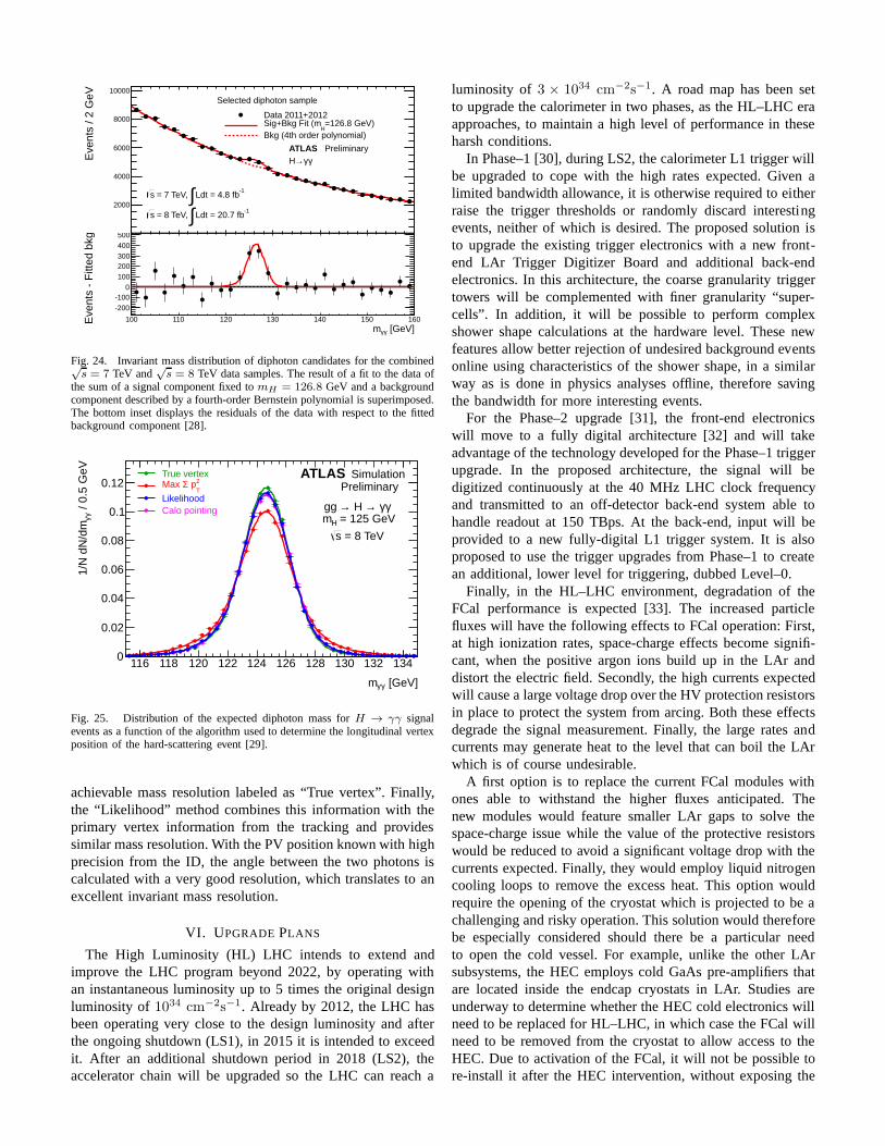
In the search for the Higgs decay to two photons, the LArcalorimeter played an especially significant role. In brief, theH → γγ analysis searches the diphoton invariant mass spec-trum for a small excess over a formidable background (Fig.24). As described in Section V-B, the calorimeter providesexcellent photon identification and jet background rejection,by exploiting its fine longitudinal segmentation, thereby im-proving the signal to background ratio. Further, the diphotoninvariant mass, defined as

mγγ =√

2E1E2 (1− cos θ)

whereE1, E2 are the two photon energies andθ is the anglebetween them, needs to be reconstructed with a very highprecision so a very small excess can be distinguished overa large background. With an excellent energy resolution, thecalorimeter ensures a very good measurement of the photonenergies. In addition, the unique capability to reconstruct thephoton direction is a significant advantage in improving theangle measurement in the high pileup environment of the LHC.More specifically, the calorimeter pointing is used to choosethe event primary vertex (PV) from a set of several tens of PVcandidates. As shown in Fig. 25, the use of the calorimeterinformation, labeled as “Calo pointing” is significantly betterthan the ID-only approach, labeled as “Max

∑

p2T

”, whichselects the PV based on the momentum of the tracks associatedwith each candidate. Further, it is very similar to the optimal

100 110 120 130 140 150 160

Eve

nts

/ 2 G

eV

2000

4000

6000

8000

10000

ATLAS Preliminaryγγ→H

-1Ldt = 4.8 fb∫ = 7 TeV, s

-1Ldt = 20.7 fb∫ = 8 TeV, s

Selected diphoton sample

Data 2011+2012=126.8 GeV)

HSig+Bkg Fit (mBkg (4th order polynomial)

[GeV]γγm100 110 120 130 140 150 160E

vent

s -

Fitt

ed b

kg

-200-100

0100200300400500

Fig. 24. Invariant mass distribution of diphoton candidates for the combined√s = 7 TeV and

√s = 8 TeV data samples. The result of a fit to the data of

the sum of a signal component fixed tomH = 126.8 GeV and a backgroundcomponent described by a fourth-order Bernstein polynomial is superimposed.The bottom inset displays the residuals of the data with respect to the fittedbackground component [28].

[GeV]γγm

116 118 120 122 124 126 128 130 132 134

/ 0.

5 G

eVγγ

1/N

dN

/dm

0

0.02

0.04

0.06

0.08

0.1

0.12True vertex

2

T pΣMax

LikelihoodCalo pointing

ATLAS SimulationPreliminary

γγ → H →gg = 125 GeVHm

= 8 TeVs

Fig. 25. Distribution of the expected diphoton mass forH → γγ signalevents as a function of the algorithm used to determine the longitudinal vertexposition of the hard-scattering event [29].

achievable mass resolution labeled as “True vertex”. Finally,the “Likelihood” method combines this information with theprimary vertex information from the tracking and providessimilar mass resolution. With the PV position known with highprecision from the ID, the angle between the two photons iscalculated with a very good resolution, which translates toanexcellent invariant mass resolution.

VI. U PGRADEPLANS

The High Luminosity (HL) LHC intends to extend andimprove the LHC program beyond 2022, by operating withan instantaneous luminosity up to 5 times the original designluminosity of 1034 cm−2s−1. Already by 2012, the LHC hasbeen operating very close to the design luminosity and afterthe ongoing shutdown (LS1), in 2015 it is intended to exceedit. After an additional shutdown period in 2018 (LS2), theaccelerator chain will be upgraded so the LHC can reach a

luminosity of 3 × 1034 cm−2s−1. A road map has been setto upgrade the calorimeter in two phases, as the HL–LHC eraapproaches, to maintain a high level of performance in theseharsh conditions.

In Phase–1 [30], during LS2, the calorimeter L1 trigger willbe upgraded to cope with the high rates expected. Given alimited bandwidth allowance, it is otherwise required to eitherraise the trigger thresholds or randomly discard interestingevents, neither of which is desired. The proposed solution isto upgrade the existing trigger electronics with a new front-end LAr Trigger Digitizer Board and additional back-endelectronics. In this architecture, the coarse granularitytriggertowers will be complemented with finer granularity “super-cells”. In addition, it will be possible to perform complexshower shape calculations at the hardware level. These newfeatures allow better rejection of undesired background eventsonline using characteristics of the shower shape, in a similarway as is done in physics analyses offline, therefore savingthe bandwidth for more interesting events.

For the Phase–2 upgrade [31], the front-end electronicswill move to a fully digital architecture [32] and will takeadvantage of the technology developed for the Phase–1 triggerupgrade. In the proposed architecture, the signal will bedigitized continuously at the 40 MHz LHC clock frequencyand transmitted to an off-detector back-end system able tohandle readout at 150 TBps. At the back-end, input will beprovided to a new fully-digital L1 trigger system. It is alsoproposed to use the trigger upgrades from Phase–1 to createan additional, lower level for triggering, dubbed Level–0.

Finally, in the HL–LHC environment, degradation of theFCal performance is expected [33]. The increased particlefluxes will have the following effects to FCal operation: First,at high ionization rates, space-charge effects become signifi-cant, when the positive argon ions build up in the LAr anddistort the electric field. Secondly, the high currents expectedwill cause a large voltage drop over the HV protection resistorsin place to protect the system from arcing. Both these effectsdegrade the signal measurement. Finally, the large rates andcurrents may generate heat to the level that can boil the LArwhich is of course undesirable.

A first option is to replace the current FCal modules withones able to withstand the higher fluxes anticipated. Thenew modules would feature smaller LAr gaps to solve thespace-charge issue while the value of the protective resistorswould be reduced to avoid a significant voltage drop with thecurrents expected. Finally, they would employ liquid nitrogencooling loops to remove the excess heat. This option wouldrequire the opening of the cryostat which is projected to be achallenging and risky operation. This solution would thereforebe especially considered should there be a particular needto open the cold vessel. For example, unlike the other LArsubsystems, the HEC employs cold GaAs pre-amplifiers thatare located inside the endcap cryostats in LAr. Studies areunderway to determine whether the HEC cold electronics willneed to be replaced for HL–LHC, in which case the FCal willneed to be removed from the cryostat to allow access to theHEC. Due to activation of the FCal, it will not be possible tore-install it after the HEC intervention, without exposingthe

personnel to unacceptable radiation levels. In this scenario,therefore, complete replacement of the modules is favored.

A second option would consist of installing an additionalwarm calorimeter (namedminiFCal) in available space in frontof the existing FCal system, closer to the interaction point.This option is attractive since it avoids the risk of openingthe cryostat cold volume and can be installed more readily,thereby saving time. Various technologies have been proposedfor the miniFCal. One of them, very radiation hard, involvingdiamond wafers as active material, has been studied to assessits linearity, uniformity and resolution. However, this option isdisfavored mainly due to its prohibiting cost. Other consideredtechnologies include xenon gas as active medium as well asfamiliar LAr technology, each with their own implementationchallenges.

Finally there is the option of not taking any action and livingwith the degraded performance and the possibility of the LArboiling at very high rates, which has yet to be explicitly ruledout. Additional studies are required to better quantify thelevelof FCal degradation to be anticipated in HL–LHC, before adecision is made taking into account detector safety, scheduleand cost.

VII. CONCLUSION

The LAr calorimeter system has performed exceptionallywell over the first few years of operation, with near optimalefficiency as well as impressive performance, contributingto the overall ATLAS performance that culminated in thediscovery in 2012 of the long sought after Higgs boson.Keeping this level of performance requires a tremendous effortby a significant number of people who intend to keep orexceed this level in the coming challenging years. Studies arecontinuing in order to improve the performance as the LHCdelivers data at unprecedented energies and rates, and ensurethat any physics that exists at the TeV-scale will be discovered.

REFERENCES

[1] G. Aad et al., “The ATLAS experiment at the CERN Large HadronCollider,” JINST, vol. 3, p. S08003, 2008.

[2] B. Aubert et al., “Construction, assembly and tests of the ATLASelectromagnetic barrel calorimeter,”Nucl.Instrum.Meth., vol. 558, no. 2,pp. 388 – 418, 2006.

[3] M. Aleksa et al., “Construction, assembly and tests of the ATLASelectromagnetic end-cap calorimeters,”JINST, vol. 3, no. 06, p. P06002,2008.

[4] D. M. Gingrich, “Construction, assembly and testing of the ATLAShadronic end-cap calorimeter,”JINST, vol. 2, no. 05, p. P05005, 2007.

[5] A. Artamonovet al., “The ATLAS Forward Calorimeter,”JINST, vol. 3,p. P02010, 2008.

[6] G. Aad et al., “Drift time measurement in the ATLAS Liquid ArgonElectromagnetic Calorimeter using cosmic muons,”Eur.Phys.J., vol.C70, pp. 755–785, 2010.

[7] N. J. Buchananet al., “ATLAS Liquid Argon calorimeter front endelectronics,”JINST, vol. 3, no. 09, p. P09003, 2008.

[8] W. E. Cleland and E. G. Stern, “Signal processing considera-tions for liquid ionization calorimeters in a high rate environment,”Nucl.Instrum.Meth., vol. A338, pp. 467–497, 1994.

[9] ETM professional control at http://www.etm.at.[10] Public LAr calorimeter plots on detector status at https://twiki.cern.ch/

twiki/bin/view/AtlasPublic/LArCaloPublicResultsDetStatus.[11] M. Adamset al., “A purity monitoring system for liquid argon calorime-

ters,” Nucl.Instrum.Meth., vol. A545, pp. 613–623, 2005.[12] Public LAr calorimeter plots for collision data at

https://twiki.cern.ch/twiki/bin/view/AtlasPublic/LArCaloPublicResults2010.

[13] “Non-collision backgrounds as measured by the atlas detector during the2010 proton-proton run,” CERN, Geneva, Tech. Rep. ATLAS-CONF-2011-137, Sep 2011.

[14] G. Aad et al., “Search for non-pointing photons in the diphoton andEmiss

Tfinal state in

√s = 7 TeV proton-proton collisions using the

ATLAS detector,” Apr 2013, submitted to Phys. Rev. D.[15] ——, “Electron performance measurements with the ATLASdetector

using the 2010 LHC proton-proton collision data,”Eur. Phys. J., vol.C72, p. 1909, 2012.

[16] M. J. Oreglia, “A study of the reactionsψ′ → γγψ,” Ph. D thesis,1980, Appendix D.

[17] J. E. Gaiser, “Charmonium spectroscopy from radiativedecays of theJ/ψ andψ′,” Ph. D thesis, 1982, Appendix F.

[18] “Electron energy response stability with time up to september 2012(hcp dataset),” CERN, Geneva, Tech. Rep. ATL-COM-PHYS-2012-1593, Nov 2012.

[19] “Electron energy response with respect to pileup in 2012 data,” CERN,Geneva, Tech. Rep. ATL-COM-PHYS-2012-1668, Nov 2012.

[20] “Expected electron performance in the ATLAS experiment,” CERN,Geneva, Tech. Rep. ATL-PHYS-PUB-2011-006, Apr 2011.

[21] “Electron identification efficiency dependence on pileup,” CERN,Geneva, Tech. Rep. ATL-COM-PHYS-2011-1636, Nov 2011.

[22] “Photon identification efficiency measurements usingZ → ℓℓγ eventsin 20.7 fb−1 of pp collisions collected by atlas at

√s = 8 tev in 2012,”

CERN, Geneva, Tech. Rep. ATL-COM-PHYS-2013-244, Feb 2013.[23] “Expected photon performance in the ATLAS experiment,” CERN,

Geneva, Tech. Rep. ATL-PHYS-PUB-2011-007, Apr 2011.[24] “Measurements of the photon identification efficiency with the ATLAS

detector using 4.9 fb1 of pp collision data collected in 2011,” CERN,Geneva, Tech. Rep. ATLAS-CONF-2012-123, Aug 2012.

[25] Electron/Gamma public results at https://atlas.web.cern.ch/Atlas/GROUPS/PHYSICS/EGAMMA/PublicPlots/20100721/display-photons/display-photons.pdf.

[26] G. Aad et al., “Observation of a new particle in the search for theStandard Model Higgs boson with the ATLAS detector at the LHC,”Phys.Lett., vol. B716, pp. 1–29, 2012.

[27] “Measurements of the properties of the Higgs-like boson in the fourlepton decay channel with the ATLAS detector using 25 fb−1 of proton-proton collision data,” CERN, Geneva, Tech. Rep. ATLAS-CONF-2013-013, Mar 2013.

[28] “Measurements of the properties of the Higgs-like boson in the twophoton decay channel with the ATLAS detector using 25fb−1 of proton-proton collision data,” CERN, Geneva, Tech. Rep. ATLAS-CONF-2013-012, Mar 2013.

[29] “Observation of an excess of events in the search for theStandard ModelHiggs boson in the gamma-gamma channel with the ATLAS detector,”CERN, Geneva, Tech. Rep. ATLAS-CONF-2012-091, Jul 2012.

[30] “Letter of intent for the Phase-I upgrade of the ATLAS experiment,”CERN, Geneva, Tech. Rep. CERN-LHCC-2011-012. LHCC-I-020,Nov2011.

[31] “Letter of intent for the Phase-II upgrade of the ATLAS experiment,”CERN, Geneva, Tech. Rep. CERN-LHCC-2012-022. LHCC-I-023,Dec2012.

[32] Timothy R Andeen, “Upgraded Readout Electronics for the ATLASLiquid Argon Calorimeters at the High Luminosity LHC,”Journal ofPhysics: Conference Series, vol. 404, no. 1, p. 012061, 2012.

[33] J. Rutherfoord, “Upgrade plans for the ATLAS Forward Calorimeter atthe HL–LHC,” Journal of Physics: Conference Series, vol. 404, no. 1,p. 012015, 2012.