PERFORMANCE OF CEMENT-FREE GEOPOLYMER CONCRETE …
165
United Arab Emirates University United Arab Emirates University Scholarworks@UAEU Scholarworks@UAEU Theses Electronic Theses and Dissertations 4-2021 PERFORMANCE OF CEMENT-FREE GEOPOLYMER CONCRETE PERFORMANCE OF CEMENT-FREE GEOPOLYMER CONCRETE MADE WITH CERAMIC WASTE POWDER USING TAGUCHI MADE WITH CERAMIC WASTE POWDER USING TAGUCHI METHOD METHOD Ponalagappan Chokkalingam Follow this and additional works at: https://scholarworks.uaeu.ac.ae/all_theses Part of the Civil Engineering Commons Recommended Citation Recommended Citation Chokkalingam, Ponalagappan, "PERFORMANCE OF CEMENT-FREE GEOPOLYMER CONCRETE MADE WITH CERAMIC WASTE POWDER USING TAGUCHI METHOD" (2021). Theses. 812. https://scholarworks.uaeu.ac.ae/all_theses/812 This Thesis is brought to you for free and open access by the Electronic Theses and Dissertations at Scholarworks@UAEU. It has been accepted for inclusion in Theses by an authorized administrator of Scholarworks@UAEU. For more information, please contact [email protected].
Transcript of PERFORMANCE OF CEMENT-FREE GEOPOLYMER CONCRETE …

United Arab Emirates University United Arab Emirates University
Scholarworks@UAEU Scholarworks@UAEU
Theses Electronic Theses and Dissertations
4-2021
PERFORMANCE OF CEMENT-FREE GEOPOLYMER CONCRETE PERFORMANCE OF CEMENT-FREE GEOPOLYMER CONCRETE
MADE WITH CERAMIC WASTE POWDER USING TAGUCHI MADE WITH CERAMIC WASTE POWDER USING TAGUCHI
METHOD METHOD
Ponalagappan Chokkalingam
Follow this and additional works at: https://scholarworks.uaeu.ac.ae/all_theses
Part of the Civil Engineering Commons
Recommended Citation Recommended Citation Chokkalingam, Ponalagappan, "PERFORMANCE OF CEMENT-FREE GEOPOLYMER CONCRETE MADE WITH CERAMIC WASTE POWDER USING TAGUCHI METHOD" (2021). Theses. 812. https://scholarworks.uaeu.ac.ae/all_theses/812
This Thesis is brought to you for free and open access by the Electronic Theses and Dissertations at Scholarworks@UAEU. It has been accepted for inclusion in Theses by an authorized administrator of Scholarworks@UAEU. For more information, please contact [email protected].

ii
Declaration of Original Work
I, Ponalagappan Chokkalingam, the undersigned, a graduate student at the United
Arab Emirates University (UAEU), and the author of this thesis entitled
“Performance of Cement-Free Geopolymer Concrete Made with Ceramic Waste
Powder Using Taguchi Method”, hereby, solemnly declare that this thesis is my
own original research work that has been done and prepared by me under the
supervision of Dr. Hilal El-Hassan, in the College of Engineering at UAEU. This
work has not previously been presented or published, or formed the basis for the
award of any academic degree, diploma or a similar title at this or any other
university. Any materials borrowed from other sources (whether published or
unpublished) and relied upon or included in my thesis have been properly cited and
acknowledged in accordance with appropriate academic conventions. I further
declare that there is no potential conflict of interest with respect to the research,
data collection, authorship, presentation and/or publication of this thesis.
Student’s Signature: Date: 18.05.2021

iii
Copyright
Copyright © 2021 Ponalagappan Chokkalingam
All Rights Reserved
iv
Advisory Committee
1) Advisor: Dr. Hilal El-Hassan
Title: Associate Professor
Department of Civil and Environmental Engineering
College of Engineering
2) Co-advisor: Professor Amr S. El-Dieb
Title: Professor
Department of Civil and Environmental Engineering
College of Engineering
v
Approval of the Master Thesis
This Master Thesis is approved by the following Examining Committee Members:
1) Advisor (Committee Chair): Dr. Hilal El-Hassan
Title: Associate Professor
Department of Civil and Environmental Engineering
College of Engineering
Signature Date
2) Member: Yaser Elhanafy Afifi
Title: Professor
Department of Chemistry
College of Science
Signature Date
3) Member (External Examiner): Dr. Mo Kim Hung
Title: Senior Lecturer
Department of Civil Engineering
Institution: University of Malaya, Malaysia
Signature Date
May 18, 2021on behalf on external examiner
Bilal.Elariss
Typewritten Text
Bilal.Elariss
Typewritten Text
Bilal.Elariss
Typewritten Text
May 18, 2021
Bilal.Elariss
Typewritten Text

18/5/2021
30/5/2021
vii
Abstract
The ceramic industry produces a substantial amount of waste during its production
processes. Recycling and reutilizing such ceramic waste is a challenge due to its
extended biodegradation period. Consequently, the ceramic industry is dedicated on
attaining a sustainable solution to dispose of this waste rather than discarding it
wastefully into landfills or stockpiles. In turn, the demand for ordinary Portland
cement has been on a steady increase, leading to concerns about the sustainability of
the construction industry. As a sustainable alternative to cement, alkali-activated
binders have been proposed owing to their ability to reduce carbon emissions,
preserve nonrenewable natural resources, and recycle industrial solid wastes. This
research aims to evaluate the feasibility of recycling ceramic waste powder (CWP) in
cement-free geopolymer concrete. Ground granulated blast furnace slag (GGBFS)
was integrated at different mass replacement percentages to enhance the performance
of said concrete and promote the use of CWP as a main component. The study
encompassed three experimental phases. The first phase characterized the as-
received materials, while the second phase involved the use of the Taguchi method to
proportion different geopolymer concrete mixes. Various factors and levels were
utilized to generate an orthogonal array of the parameters. Mixture proportions were
optimized to attain superior mechanical and short-term durability performance.
Further augmentation was performed in the third phase through multi-response
optimization using the Best Worst Method (BWM) and Technique for Order
Preference by Similarity to Ideal Solution (TOPSIS) based Taguchi method. The
optimized CWP-GGBFS blended geopolymer concrete mix made with a binder
content of 450 kg/m3, GGBFS replacement percentage of 60%, alkaline-activator

viii
solution-to-binder ratio of 0.50, sodium silicate-to-sodium hydroxide ratio of 1.5, and
molarity of SH solution of 10 M exhibited a compressive strength of 80.3 MPa, a
flexural strength of 5.72 MPa, and a splitting tensile strength of 3.81 MPa, among
other properties. Nevertheless, it was possible to produce a concrete made with 80%
CWP with acceptable performance for structural applications. Accordingly, this work
highlights the feasibility of producing geopolymer concrete made with CWP to
promote the recycling of industrial solid waste, reduce carbon emissions, and
preserve natural resources. Recommendations for future investigations were also
included.
Keywords: Ceramic waste powder, ground granulated blast furnace slag,
geopolymer concrete, Taguchi method, BWM, TOPSIS, mechanical performance,
durability performance.

ix
Title and Abstract (in Arabic)
سمنت المصنوعة من مسحوق نفايات داء الخرسانة الجيوبوليمرية الخالية من الإأ
طريقة تاجوتشي السيراميك باستخدام
صالملخ
أثناء إنتاجها. تمثل إعادة تدوير نفايات السيراميك تحديا تنتج صناعة السيراميك كمية كبيرة من النفايات
، تركز صناعات السيراميك على إيجاد حل مستدام للتخلص ذلكبسبب فترة التحلل البيولوجي الطويلة. ل
، أدت الزيادة في مدافن النفايات. وفي الوقت نفسه في أكوام التخزين أو هامن نفاياتها بدلا من هدر
الأسمنت البورتلاندي إلى زيادة المخاوف بشأن استدامة صناعة البناء. تم اقتراح مواد الطلب على
، وتقليل غير متجددةالى الموارد الطبيعية كبديل مستدام للأسمنت نظرا لقدرتها على الحفاظ عل ةقلوي
ث إلى دراسة الصلبة. وفقا لذلك، يهدف هذا البحالصناعية انبعاثات الكربون، وإعادة تدوير النفايات
في الخرسانة غير القابل للتحلل الحيوي(CWP) إعادة استخدام مسحوق نفايات السيراميك قدرة
بنسب مختلفة من استبدال (GGBFS)تم دمج خبث أفران الصهر .الجيوبوليمرية الخالية من الأسمنت
اشتملت الدراسة على كمكون رئيسي. CWP الكتلة لتحسين أداء الخرسانة المذكورة وتعزيز استخدام
المواد المستلمة، بينما تضمنت المرحلة الثانية استخدام درست خواص ثلاث مراحل. المرحلة الأولى
طريقة تاجوشي لتصميم خلطات خرسانية جيوبوليمرية مختلفة. تم استخدام عوامل ومستويات مختلفة
قدرة . تم تحسين نسب الخليط لتحقيق أداء ميكانيكي متفوق المعطياتلإنشاء مجموعة متعامدة من
. تم إجراء المزيد من التعزيز في المرحلة الثالثة من خلال التحمل مع الزمن جسدة على المدى القصير
وتقنية تفضيل الطلب عن طريق التشابه مع طريقة BWMتحسين الاستجابة المتعددة باستخدام
Taguchi مثاليالقائمة على الحل ال (TOPSIS). مزيج الخرسانة الجيوبوليمر الممزوج المحسن
CWP-GGBFS نسبة استبدال 3كجم / م 054المصنوع بمحتوى رابط يبلغ ، GGBFS 04بنسبة ٪
، نسبة سيليكات الصوديوم إلى هيدروكسيد 4.54 محتوى الرابط، محلول المنشط القلوي إلى
MPa 34.3قوة ضغط تبلغ M 54 لـ روكسيد الصودبومهيد محلول قلوية، وأظهرت 5.5الصوديوم
، من بين خصائص أخرى. ومع MPa 3.35، وقوة شد انقسام تبلغ MPa 5.52انثناء تبلغ ، وقوة

x
بأداء مقبول للتطبيقات الإنشائية. وفقا CWP ٪ من34ذلك ، كان من الممكن إنتاج الخرسانة بنسبة
لتعزيز CWP جدوى إنتاج خرسانة جيوبوليمر مصنوعة منلذلك ، يسلط هذا العمل الضوء على
إعادة تدوير النفايات الصلبة الصناعية ، وتقليل انبعاثات الكربون ، والحفاظ على الموارد الطبيعية. كما
.المستقبلية للدراساتتم تضمين توصيات
الخرسانة الجيوبوليمرية ، مسحوق نفايات السيراميك ، خبث أفران الصهر، : مفاهيم البحث الرئيسية
، الخواص الميكانيكية ، خواص التحمل مع الزمن. BWM ،TOPSISطريقة تاجوتشي ،

xi
Acknowledgements
I would like to express my sincere thanks and admiration to my advisor, Dr. Hilal El-
Hassan who has given me endless support, patient supervision, expert guidance and
continuous encouragement during my research works. I was kept on track by his
determination to complete this work more constructively. I would like to thank him
also for the friendly environment he has created for me and the invaluable advice I
received from him.
Deep gratitude goes to the people who brought me in to life and dedicated their lives
to my well-being and happiness. I would like to thank my family for the invaluable
encouragement, unconditional guidance that I have received from them in all
circumstances. I would like to express my sincere thanks to them for believing in me,
sharing their life experience with me and motivating me to resolve the challenges
that I have faced. I am deeply grateful for their blessings, which have always been
the source of inspiration to achieve any success in my life. Without their constant
support it would have been difficult to complete this study.
I would like to thank Eng. Abdel Rahman Alsallamin and Mr. Faisal Abdul Wahab
from UAE University’s concrete laboratory for their assistance, support and patience
during this study.
The project is financially supported by the United Arab University (UAEU) (Grant
Number 31N322). The contribution of UAEU is greatly appreciated.

xii
Dedication
To my beloved parents and family

xiii
Table of Contents
Title ..................................................................................................................................... i
Declaration of Original Work ........................................................................................... ii
Copyright ......................................................................................................................... iii
Advisory Committee ......................................................................................................... iv
Approval of the Master Thesis ........................................................................................... v
Abstract ........................................................................................................................... vii
Title and Abstract (in Arabic) ........................................................................................... ix
Acknowledgements ........................................................................................................... xi
Dedication ....................................................................................................................... xii
Table of Contents ........................................................................................................... xiii
List of Tables................................................................................................................... xvi
List of Figures .............................................................................................................. xviii
List of Abbreviations........................................................................................................ xx
Chapter 1: Introduction ...................................................................................................... 1
1.1 Overview .......................................................................................................... 1
1.2 Scope and Objectives ....................................................................................... 2
1.3 Methodology and Approach ............................................................................. 3
1.4 Outline and Organization of the Thesis ........................................................... 4
1.5 Research Significance (or Impact Statement) .................................................. 5
Chapter 2: Literature Review ............................................................................................. 7
2.1 Introduction ...................................................................................................... 7
2.2 Use of Ceramic Waste in Mortar/Concrete ...................................................... 7
2.2.1 Ceramic Waste as Cement Replacement in
Mortar/Concrete ................................................................................... 13
2.2.2 Ceramic Waste as Coarse Aggregate Replacement in
Mortar/Concrete ................................................................................... 17
2.2.3 Ceramic Waste as Fine Aggregate Replacement in
Mortar/Concrete ................................................................................... 21
2.3 Geopolymer Mortar/Concrete ........................................................................ 24
2.4 Taguchi Method in Concrete .......................................................................... 33
Chapter 3: Experimental Program .................................................................................... 36
3.1 Introduction .................................................................................................... 36
3.2 Test Program .................................................................................................. 36
3.3 As-Received Material Properties ................................................................... 38
xiv
3.3.1 Binding Material .................................................................................. 38
3.3.2 Coarse Aggregates................................................................................ 43
3.3.3 Fine Aggregates.................................................................................... 44
3.3.4 Alkaline Activators .............................................................................. 45
3.3.5 Superplasticizer .................................................................................... 46
3.4 Concrete Mixture Proportions ........................................................................ 46
3.4.1 Selection of Optimal Mixtures by Taguchi Method............................. 47
3.4.2 Control Mix C1 with 100% CWP ........................................................ 48
3.4.3 Control Mix C2 with 100% GGBFS .................................................... 49
3.5 Sample Preparation ........................................................................................ 49
3.6 Concrete Testing Methodology ...................................................................... 50
3.6.1 Compressive Strength .......................................................................... 51
3.6.2 Modulus of Elasticity ........................................................................... 52
3.6.3 Splitting Tensile Strength ..................................................................... 52
3.6.4 Flexural Strength .................................................................................. 53
3.6.5 Bulk Resistivity .................................................................................... 54
3.6.6 Ultrasonic Pulse Velocity ..................................................................... 55
3.6.7 Water Absorption ................................................................................ 56
3.6.8 Sorptivity .............................................................................................. 56
3.6.9 Abrasion Resistance ............................................................................. 57
3.7 Optimization Methodology ............................................................................ 58
3.7.1 Taguchi Method ................................................................................... 61
3.7.2 Taguchi Optimization by Best Worst Method ..................................... 62
3.7.3 Taguchi Optimization by TOPSIS Method .......................................... 64
Chapter 4: Results and Discussion ................................................................................... 67
4.1 Introduction .................................................................................................... 67
4.2 Experimental Results ..................................................................................... 67
4.2.1 Fresh and Hardened Geopolymer Concrete Density ............................ 67
4.2.2 Water Absorption and Sorptivity ......................................................... 69
4.2.3 Compressive Strength .......................................................................... 72
4.2.4 Modulus of Elasticity ........................................................................... 76
4.2.5 Splitting Tensile Strength ..................................................................... 79
4.2.6 Flexural Strength .................................................................................. 84
4.2.7 Bulk Resistivity .................................................................................... 87
4.2.8 Ultrasonic Pulse Velocity ..................................................................... 89
4.2.9 Abrasion Resistance ............................................................................. 90
Chapter 5: Optimization of Mixture Proportions ............................................................. 93
5.1 Optimum Design by Taguchi Method ........................................................... 93
5.2 Taguchi Optimization by Best Worst Method ............................................... 97
5.2.1 Nine Quality Criteria ............................................................................ 97
5.2.2 Five Quality Criteria........................................................................... 103
5.2.3 Two Quality Criteria .......................................................................... 107

xv
5.3 Taguchi Optimization by TOPSIS Method .................................................. 112
5.3.1 Nine Quality Criteria .......................................................................... 112
5.3.2 Five and Two Quality Criteria ........................................................... 116
5.4 Comparison of Results from Taguchi, BWM, and TOPSIS
Optimized Method....................................................................................... 122
5.5 Validation of the Optimized Geopolymer Concrete Mix ............................. 123
Chapter 6: Conclusions and Recommendations ............................................................. 125
6.1 Introduction .................................................................................................. 125
6.2 Limitations ................................................................................................... 126
6.3 Conclusions .................................................................................................. 126
6.4 Recommendations for Future Studies .......................................................... 130
References ...................................................................................................................... 132
xvi
List of Tables
Table 1: Summary of previous studies using ceramic waste as concrete
ingredient replacement ......................................................................................... 8
Table 2: Summary of previous studies related to geopolymer concrete .......................... 28
Table 3: Experimental Test Matrix with designated factors and Levels .......................... 37
Table 4: Chemical composition of CWP and GGBFS ..................................................... 40
Table 5: Physical properties of coarse and fine aggregates ............................................. 44
Table 6: Taguchi factors and levels for CWP geopolymer concrete mixes ..................... 47
Table 7: Design mixtures for Taguchi optimization of geopolymer concrete
(kg/m3) ............................................................................................................... 48
Table 8: List of quality characteristics, standards and samples used, and age
of testing............................................................................................................. 51
Table 9: Scale rate for quality criteria .............................................................................. 62
Table 10: Fresh and hardened density of geopolymer concrete ....................................... 69
Table 11: Water absorption and initial rate of water absorption of CWPGC .................. 70
Table 12: Compressive strength of geopolymer concrete cylinders and cubes ............... 74
Table 13: Factors and modulus of elasticity of geopolymer concrete mixes ................... 78
Table 14: Splitting tensile strength of geopolymer mixtures ........................................... 83
Table 15: Flexural strength of geopolymer concrete ....................................................... 85
Table 16: Bulk resistivity and UPV of geopolymer concrete mixes ................................ 88
Table 17: Contribution of each factor towards cylinder compressive strength ............... 93
Table 18: Response Table for Signal-to-Noise Ratios ..................................................... 96
Table 19: Selected nine quality criteria, target value, and best and worst ....................... 98
Table 20: Comparision of best quality criteria to other eight quality criteria .................. 98
Table 21: Comparision of worst quality criteria to other eight quality criteria ............... 98
Table 22: Weights of the nine quality criteria .................................................................. 98
Table 23: Experimental results of Taguchi array experiments ...................................... 100
Table 24: Comparison of best experiments to other experiments with respect
to each of the nine quality criteria ................................................................. 101
Table 25: The comparison of others to worst experiments with respect to each
of the nine quality criteria. ............................................................................. 101
Table 26: The relative weight of each experiment with respect to each of the
nine quality characteristics ............................................................................ 102
Table 27: Total weight and S/N ratios for each experiment (nine quality
criteria)........................................................................................................... 103
Table 28: Selected five quality criteria, target value, and best and worst
experiment ..................................................................................................... 104
Table 29: Comparison of best quality criteria to other four quality criteria .................. 104
Table 30: Comparison of worst quality criteria to other four quality criteria ................ 104
Table 31: Weights of the five quality criteria ................................................................ 104

xvii
Table 32: Comparison of best experiments to other experiments with respect
to each of the five quality criteria .................................................................. 105
Table 33: The comparison of others to worst experiments with respect to
each of the five quality criteria. ..................................................................... 105
Table 34: The relative weight of each experiment with respect to each of the
five quality characteristics ............................................................................. 106
Table 35: Total weight and S/N ratios for each experiment
(five quality criteria) ...................................................................................... 106
Table 36: Selected five quality criteria, target value, and best and worst
experiment ..................................................................................................... 108
Table 37: Comparison of best quality criteria to the other quality criteria .................... 108
Table 38: Comparison of worst quality criteria to the other quality criteria .................. 108
Table 39: Weights of the two quality criteria................................................................. 108
Table 40: Comparison of best experiments to other experiments with respect
to each of the two quality criteria. ................................................................. 109
Table 41: The comparison of others to worst experiments with respect to
each of the two quality criteria ..................................................................... 109
Table 42: The relative weight of each experiment with respect to each of the
two quality characteristics ............................................................................. 110
Table 43: Total weight and its S/N ratios for each experiment
(two quality criteria) ...................................................................................... 111
Table 44: Contribution of factors in the three BWM-based Taguchi
methods .......................................................................................................... 112
Table 45: S/N ratios decision matrix for nine quality criteria ........................................ 113
Table 46: Normalized decision matrix for nine quality criteria ..................................... 114
Table 47: Weighted normalized decision matrix for nine quality criteria ..................... 115
Table 48: Normalized decision matrix for five quality criteria ...................................... 117
Table 49: Weighted normalized decision matrix for five quality criteria ...................... 118
Table 50: Normalized decision matrix for two quality criteria ...................................... 119
Table 51: Weighted normalized decision matrix for two quality criteria ...................... 120
Table 52: Contribution of the factors in the three TOPSIS-based Taguchi
methods .......................................................................................................... 121
Table 53: Optimum levels of factor obtained using Taguchi, BWM, and
TOPSIS method ............................................................................................. 122
Table 54: Quality criteria values and improvement in optimal mixture design ............. 124

xviii
List of Figures
Figure 1: Particle size distribution of CWP ..................................................................... 39
Figure 2: Dried and ground ceramic waste powder ......................................................... 40
Figure 3: SEM micrograph of ground CWP .................................................................... 41
Figure 4: XRD pattern of CWP ........................................................................................ 41
Figure 5: As-received GGBFS ......................................................................................... 42
Figure 6: Particle size distribution graph, SEM micrograph, and XRD
pattern of GGBFS ........................................................................................... 43
Figure 7: Particle size distribution graph for coarse aggregate ........................................ 44
Figure 8: Particle size distribution of dune sand .............................................................. 45
Figure 9: SEM and XRD pattern for dune sand ............................................................... 45
Figure 10: NaOH flakes, Sodium silicate and Superplasticizer ....................................... 46
Figure 11: Geopolymer concrete mixing and sample preparation ................................... 50
Figure 12: Compressive testing of CWP-GGBFS geopolymer cube and
cylinder specimens ......................................................................................... 52
Figure 13: Splitting tensile test ........................................................................................ 53
Figure 14: Geopolymer concrete prism specimens prior to a flexure test ....................... 54
Figure 15: Bulk resistivity test ......................................................................................... 55
Figure 16: Water absorption test ...................................................................................... 56
Figure 17: Sorptivity test on geopolymer concrete disc specimens ................................. 57
Figure 18: Weighing of specimen, Specimen after 500 revolutions in the
LA abrasion machine ..................................................................................... 58
Figure 19: Optimization methodology proposal.. ............................................................ 60
Figure 20: Schematic of the BWM model ....................................................................... 64
Figure 21: Relationship between fresh and hardened geopolymer concrete
density ............................................................................................................ 68
Figure 22: Development of absorption with time for mixes.............................................71
Figure 23: Compressive strength development of CWPGC with different
ceramic percentages ....................................................................................... 75
Figure 24: Relationship between the 28-day cylinder and cube compressive
strength ........................................................................................................... 76
Figure 25: Typical stress-strain curves of geopolymer concrete mixes with
CWP-to-GGBFS ratio .................................................................................... 80
Figure 26: Relationship between modulus of elasticity and compressive
strength of 28-day geopolymer concrete ....................................................... 81
Figure 27: Predicted versus experimental values of Ec .................................................... 81
Figure 28: Correlation between splitting tensile strength and compressive
strength ........................................................................................................... 83
Figure 29: Predicted and experimental splitting tensile strength ..................................... 84
Figure 30: Relationship between flexural and compressive strength............................... 86
Figure 31: Experimental versus predicted flexural strength ............................................ 87
xix
Figure 32: Bulk resistivity versus cylinder compressive strength of
geopolymer concrete ..................................................................................... 88
Figure 33: Relationship between UPV and compressive strength f’c .............................. 90
Figure 34: Abrasion mass loss of geopolymer concrete mixes ........................................ 92
Figure 35: Relationship between abrasion mass loss after 500 revolutions
and compressive strength .............................................................................. 92
Figure 36: Combined impact of factors and their levels on the cylinder
compressive strength of geopolymer concrete .............................................. 95
Figure 37: Signal-to-noise ratios of Taguchi design for cylinder compressive
strength ........................................................................................................... 96
Figure 38: S/N Ratio plot of nine quality criteria (Q1 to Q9) using BWM
based Taguchi method .................................................................................. 102
Figure 39: S/N Ratio plot of Five quality criteria (Q1, Q2, Q5, Q6, and Q8)
using BWM-based Taguchi method ............................................................. 107
Figure 40: SN Ratio plot of Two quality criteria (Q1 and Q2) using
BWM-based Taguchi method ..................................................................... 111
Figure 41: Optimal level for each factor by TOPSIS optimised Taguchi
method considering all quality criteria (Q1 to Q9) ...................................... 116
Figure 42: Optimal level for each factor by TOPSIS optimised Taguchi
method considering Q1, Q2, Q5, Q6, and Q8 quality criteria ..................... 119
Figure 43: Optimal level for each factor by TOPSIS-optimized Taguchi
method considering Q1 and Q2 quality criteria ........................................... 121
xx
List of Abbreviations
AAGT Alkaline Activated Mortar Using GGBFS and Natural Pozzolan
AAM Alkali Activated Mortars
AAS Alkali-Activator Solution
AASC Alkali-Activated Slag Concrete
ACI American Concrete Institute
ANOVA Analysis of Variance
AS Australian Standards
ASTM American Society for Testing and Materials
b Width of Specimen
BR Bulk Resistivity
BS British Standards
BWM Best Worst Method
CB Ceramic Bricks
CBP Crushed Basaltic Pumice
CC Crushed Ceramic
Ci Ranking score
CWP Ceramic Waste Powder
CWPGC Ceramic Waste Powder Geopolymer Concrete
D Diameter of Specimen
d Depth of Specimen
D Decision Matrix
DTA Differential Thermal Analysis
Ec Modulus of Elasticity of Concrete
xxi
EDS Energy Dispersive Spectroscopy System
FA Fly Ash
f'c Cylinder Compressive Strength
fcu Cube Compressive Strength
FESEM Field Emission Scanning Microscopic
fr Flexural Strength
fsp Splitting Tensile Strength
FTIR Fourier Transform Infrared
GGBFS Ground Granulated Blast Furnace Slag
GPC Geopolymer Concrete
HSSCC High Strength Self-Consolidated Concrete
L Length of Specimen
LFS Ladle Furnace Slag
NDT Non-Destructive Test
NIS Negative Ideal Solution
OPC Ordinary Portland Cement
P Applied Load
PCC Portland Cement Concrete
PCE Polycarboxylic Ether
PIS Positive ideal Solution
rij Vector Normalization
S/N Signal-to-Noise Ratio
SCGPC Self-Compacting Geopolymer Concrete
SCM Supplementary Cementitious Materials

xxii
SEM Scanning Electron Microscope
SH Sodium Hydroxide
SS Sodium Silicate
SSA Specific Surface Area
SSD Saturated Surface Dry
SW Sanitary Ware
TGA Thermogravimetric Analysis
TOPSIS Technique for Order Preference by Similarity to Ideal Solution
UPV Ultrasonic Pulse Velocity
V Normalized Decision Matrix
WSOF White Stoneware Once Fired
WSTF White Stoneware Twice Fired
XRD X-Ray Diffraction
XRF X-ray Fluorescence
ν Velocity
ρf Fresh Concrete Density
ρh Hardened Concrete Density

1
Chapter 1: Introduction
1.1 Overview
Portland cement is commonly used as the main binding agent in concrete
products. Its production consumes a tremendous amount of energy, reduces non-
renewable natural resources, and releases a substantial amount of greenhouse gases
[1]. Indeed, the cement industry alone accounts for 5-7 percent of global CO2
emissions [2], leading to an increase in atmospheric CO2 concentration [3, 4].
Additionally, the continuous population growth and infrastructure development are
instigating a pressing need for more concrete, thereby escalating its adverse
environmental and ecological impacts. Therefore, finding alternative materials that
can serve as binders in concrete products is critical.
Scientists and environmentalists have suggested the utilization of
supplementary cementitious materials (SCMs) to partially replace cement. Indeed, if
less cement could be employed as the binding agent in concrete, it could alleviate the
negative effects of concrete production, including carbon emission and consumption
of non-renewable natural resources. Nevertheless, such a solution would only
postpone the inevitable pollution of the environment and depletion of raw materials
unless cement could be completely replaced. Such complete replacement of cement
in concrete was successfully implemented in the manufacture of inorganic alkali-
activated geopolymer concrete. In this novel production, a precursor binding
material, such as fly ash (FA), ground granulated blast furnace slag (GGBFS), and
others, was activated by an alkaline solution. Thus, it eliminates the need for cement
and reduces its associated detrimental impact on the environment. In fact, the
sustainability of this innovative concrete product has been examined in a recent
2
lifecycle assessment study that reported at least a 25% reduction in greenhouse gas
emissions, energy consumption, and water utilization [2].
In addition to the reduction in cement consumption, geopolymer offers other
important benefits. The precursor binders are industrial by-products, which are
typically disposed of in landfills or stockpiled. As such, their use as a binding agent
in geopolymer serves as a sustainable form of waste management. Of the various
industry practices around the world, ceramic tile manufacturing has reached a global
production of over 12 billion square meters. Yet, its production is associated with the
generation of ceramic waste powder (CWP) at a rate of 19 kg/m2 during the final
polishing process. As such, the global CWP generation exceeds 228 million tons [5].
Owing to its highly crystalline alumina silicate structure, CWP may be used as a
binding agent in the production of alkali-activated geopolymer concrete and mortars
for structural applications. However, such an investigation has not been carried out
yet.
1.2 Scope and Objectives
The main aim of this research is to develop and evaluate the performance of
geopolymer concrete made with CWP. Based on the trial mixes, it was found that
using CWP alone in the mix did not result in adequate workability or compressive
strength. Therefore, slag (GGBFS) was used as in partial replacement of CWP to
promote the geopolymerization reaction and enhance the performance. Dune sand
replaced natural crushed stone as a more sustainable fine aggregate. The mixture
proportions were optimized following the comprehensive evaluation of the physical,
mechanical, and short-term durability properties. The specific objectives of this
project are as follows:

3
Design geopolymer concrete mixture proportions based on a parametric
orthogonal array developed using the Taguchi method.
Evaluate the mechanical properties of the different geopolymer concrete
mixes.
Investigate the effect of different geopolymer concrete mix proportions on
the short-term durability properties.
Optimize the mixture proportions following basic Taguchi, BWM, and
TOPSIS-based Taguchi optimization methods.
1.3 Methodology and Approach
In this study, the Taguchi method was used to optimize the mix design of
geopolymer concrete and maximize the performance. The Taguchi experimental
design was performed through five variables, each at four levels, including binder
content (400, 450, 500, and 550 kg/m3), CWP replacement percentage by GGBFS
(20, 40, 60, and 80%, by mass), alkali-activator solution (AAS)-to-binder ratio (0.5,
0.55, 0.6, and 0.65), sodium silicate-to-sodium hydroxide ratio (1.0, 1.5, 2.0, and
2.5), and sodium hydroxide solution molarity or molar concentration (8, 10, 12, and
14M). A total of 16 mixes were prepared based on the L16 array obtained using the
Taguchi method. Yet, if the Taguchi method were not used, a total of 1024
experiments would be needed. Hardened concrete properties such as compressive
strength, abrasion resistance, splitting tensile strength, flexure strength, and
ultrasonic pulse velocity were measured. Durability characteristics were assessed by
testing for water absorption, sorptivity, and bulk resistivity. Later, the Best Worst
Method (BWM) and Technique for Order Preference by Similarity to Ideal Solution
(TOPSIS) based Taguchi optimization methods were used to determine the optimum

4
mixture proportions of the CWP-GGBFS blended geopolymer concrete that would
maximize the different performance criteria.
1.4 Outline and Organization of the Thesis
This thesis is organized into the following six chapters:
Chapter 1: A brief introduction about the problem statement is given, followed by the
research objectives, methodology, significance, and organization of the thesis.
Chapter 2: An extensive and detailed literature review on the use of different types
and quantities of ceramic waste as cement and aggregate replacement in the
production of concrete is provided. A background on geopolymers is also furnished.
Chapter 3: A detailed description of the properties of the as-received material used to
prepare the concrete mixtures, concrete mixtures proportions, sample preparation,
and experimental tests is given.
Chapter 4: The test results of geopolymer concrete mixes are presented and
discussed, including mechanical properties (compressive strength, split tensile
strength, and flexural strength) and durability properties (abrasion resistance, bulk
resistivity, sorptivity, UPV, and water absorption). Correlations among these
properties are also provided.
Chapter 5: Geopolymer concrete mixture proportions are optimized using the basic
Taguchi method and multi-response optimization techniques, including BWM and
TOPSIS-based Taguchi methods.
Chapter 6: Main conclusions and limitations of the work and recommendations for
future studies on the use of CWP in geopolymer concrete mixtures are described.

5
1.5 Research Significance (or Impact Statement)
The increasing demand for concrete is owed to population growth and the
rapid development of the global economy. Many natural resources have been
consumed in the production of concrete and its basic component, cement. In addition
to its ecological impact, manufacturing cement is associated with the release of large
amounts of carbon dioxide into the atmosphere. In fact, the concentration of CO2 in
the atmosphere has increased by 42% in the past 200 years. Efforts have been made
to alleviate these CO2 emissions by developing environment-friendly construction
materials. Supplementary cementitious materials (SCMs) have been utilized in the
past to partially replace cement. However, unless the cement can be completely
replaced, the pollution of the environment and depletion of raw materials will not
halt.
On one occasion, full cement replacement was attained in the production of
an inorganic alkali-activated geopolymer. This novel material promises to reduce
carbon emissions and mitigate the consumption of natural resources. As the main
precursor binders are in the form of industrial by-products, it also offers to recycle
these wastes rather than disposing of them in landfills or stockpiles. Past research has
extensively investigated geopolymers with a focus on metakaolin, GGBFS, fly ash,
and other materials. Yet, ceramic waste powder, which is a by-product of ceramic
manufacture, has not been examined as a binder for geopolymer concrete. The partial
replacement of CWP with GGBFS in such concrete has also not been investigated.
Further, performance-based optimum mixture proportions of CWP-GGBFS blended
geopolymer concrete have not been developed.

6
This research aims to provide experimental evidence for the potential
utilization of CWP and GGBFS in blended geopolymer concrete. The physical,
mechanical, and durability properties of this novel geopolymer concrete will be
evaluated. The proposed geopolymer concrete will provide a novel sustainable
solution to globally renowned environmental issues, namely the depletion of natural
resources and emission of carbon dioxide. It will also beneficially recycle industrial
by-products in construction materials and applications rather than wastefully
discarding them into landfills and stockpiles.

7
Chapter 2: Literature Review
2.1 Introduction
This chapter summarizes the relevant research work related to the use of
ceramic waste in concrete mixtures. It also provides an overview of geopolymer
concrete and the use of the Taguchi method and other multi-response optimization
techniques in optimizing mixture proportions. Reuse of ceramic wastes in concrete as
aggregate and cement replacement has been an area of focused investigations, owing
to its similarities to other forms of industrial by-products and SCMs. In fact, its use
in concrete can enhance its sustainability and reduce its environmental footprint.
2.2 Use of Ceramic Waste in Mortar/Concrete
Based on the materials used in their production, ceramic ware can be
separated into two groups [6]. Group 1 includes products of burned red clay (bricks,
structural wall, and floor tiles, roof tiles), while Group 2 comprises products made of
white clay, such as technical ceramics (ceramic electrical insulators), ceramic
sanitary ware (washbowls, lavatory pans, bidets, and bathtubs), and medical and
laboratory vessels.
Past literature has widely investigated the use of ceramic waste as a cement or
aggregate replacement in conventional concrete and are explained in the below
sections. Table 1 summarizes the available previous studies related to the use of
recycled ceramic waste material in concrete mixtures as binding materials, fine
aggregate, and coarse aggregate.

8
Table 1: Summary of previous studies using ceramic waste as concrete ingredient
replacement
Author [6] [7] [8] [9] [10] [11]
Type of
Ceramic
Waste Used
for Study
Electrical Industrial Waste
Stone/Table/Ware/White Ceramic Wall
/Floor Tiles
Red ceramic Wall Tiles
Sanitary Ware Waste
Earthen Ware
Bricks
Blocks
Roof Tiles
Mineral Admixture
Ceramic
Waste
Replacing
Cement
Coarse Aggregate
Fine Aggregate
Ceramic
Waste Used
in
Conventional Mortar
Geopolymer Mortar
Conventional Concrete
Geopolymer Concrete
Fresh
or Physical
Properties
Fratini Test
Slump or similar
Density
Air Content
Consistency
Setting Time
Mechanical
or Durability
Properties
Compressive Strength
Splitting Tensile Strength
Flexural Strength
Abrasion Resistance
Water Absorption
Sorptivity
Ultrasonic Pulse Velocity
Electrical Resistivity
/Thermal Conductivity
RCPT
Sulphate Resistance
Modulus of Elasticity
Expansion
Drying Shrinkage
Volume of
Voids/Permeable Pores
Dynamic Modulus
Leaching Test
Water Resistance
Frost Resistance
Flow Number

9
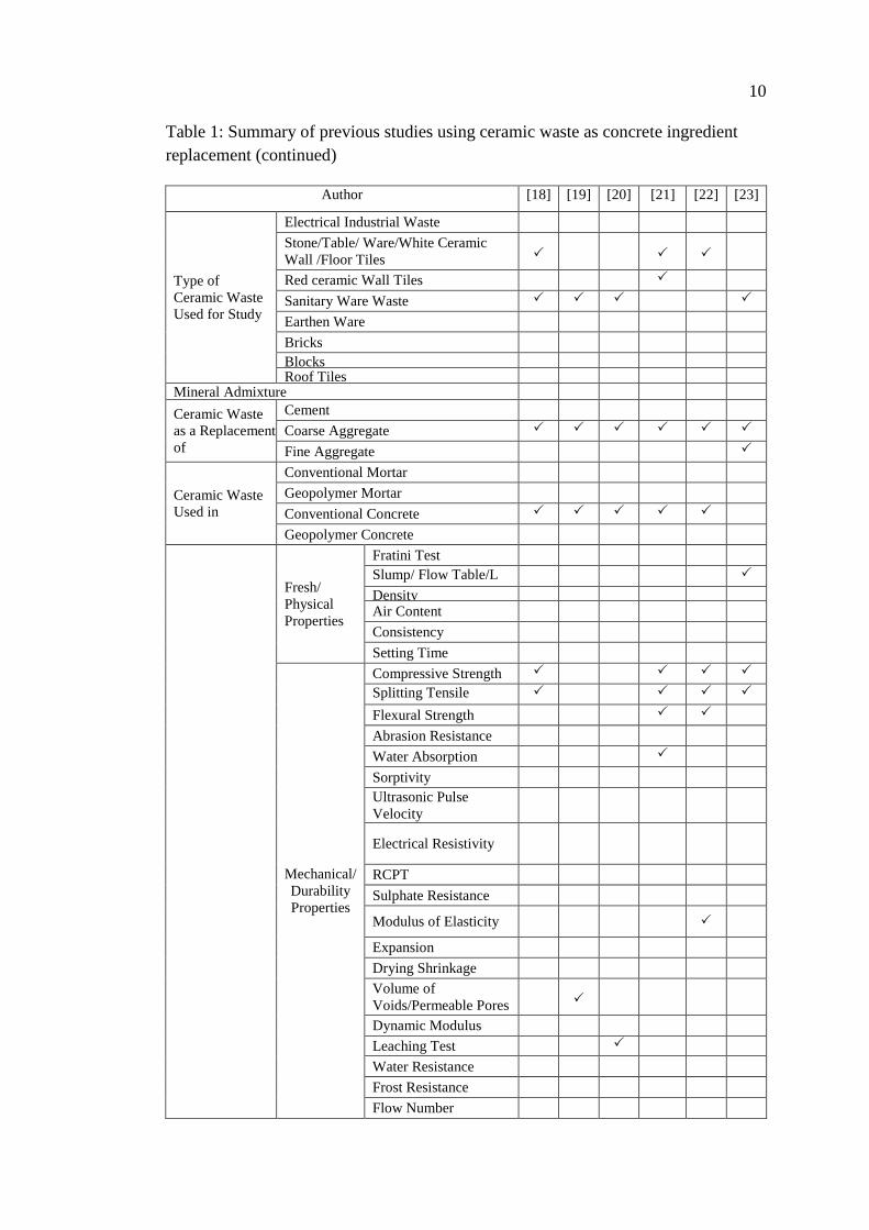
Table 1: Summary of previous studies using ceramic waste as concrete ingredient
replacement (continued)
Author [12] [13] [14] [15] [16] [17]
Type of
Ceramic
Waste Used
for Study
Electrical Industrial Waste
Stone/Table/ Ware/White Ceramic
Wall /Floor Tiles
Red ceramic Wall Tiles
Sanitary Ware Waste
Earthen Ware
Bricks
Blocks
Roof Tiles
Mineral Admixture
GB
GF
S&
Fly
Ash
waste
sand
Ceramic
Waste as a
Replacement
of
Cement
Coarse Aggregate
Fine Aggregate
Ceramic
Waste Used
in
Conventional Mortar
Geopolymer Mortar
Conventional Concrete
Geopolymer Concrete
Fresh/
Physical
Properties
Fratini Test
Slump/ Flow
Table/L Box/ J
Ring
Density
Air Content
Consistency
Setting Time
Mechanical/
Durability
Properties
Compressive
Strength
Splitting Tensile
Strength
Flexural Strength
Abrasion
Resistance
Water Absorption
Sorptivity
Ultrasonic Pulse
Velocity
Electrical
Resistivity
/Thermal
Conductivity
RCPT
Sulphate Resistance
Modulus of
Elasticity
Expansion
Drying Shrinkage
Volume of
Voids/Permeable
Pores
Dynamic Modulus
Leaching Test
Water Resistance
Frost Resistance
Flow Number
10
Table 1: Summary of previous studies using ceramic waste as concrete ingredient
replacement (continued)
Author [18] [19] [20] [21] [22] [23]
Type of
Ceramic Waste
Used for Study
Electrical Industrial Waste
Stone/Table/ Ware/White Ceramic
Wall /Floor Tiles
Red ceramic Wall Tiles
Sanitary Ware Waste
Earthen Ware
Bricks
Blocks
Roof Tiles
Mineral Admixture
Ceramic Waste
as a Replacement
of
Cement
Coarse Aggregate
Fine Aggregate
Ceramic Waste
Used in
Conventional Mortar
Geopolymer Mortar
Conventional Concrete
Geopolymer Concrete
Fresh/
Physical
Properties
Fratini Test
Slump/ Flow Table/L
Box/ J Ring
Density
Air Content
Consistency
Setting Time
Mechanical/
Durability
Properties
Compressive Strength
Splitting Tensile
Strength
Flexural Strength
Abrasion Resistance
Water Absorption
Sorptivity
Ultrasonic Pulse
Velocity
Electrical Resistivity
RCPT
Sulphate Resistance
Modulus of Elasticity
Expansion
Drying Shrinkage
Volume of
Voids/Permeable Pores
Dynamic Modulus
Leaching Test
Water Resistance
Frost Resistance
Flow Number

11
Table 1: Summary of previous studies using ceramic waste as concrete ingredient
replacement (continued)
Author [24] [25] [26] [27] [2
8]
[29]
Type of
Ceramic
Waste Used
for Study
Electrical Industrial Waste
Stone/Table/ Ware/White Ceramic
Wall /Floor Tiles
Red ceramic Wall Tiles
Sanitary Ware Waste
Earthen Ware
Bricks
Blocks
Roof Tiles
Mineral Admixture Laterite
Ceramic
Waste as a
Replacement
of
Cement
Coarse Aggregate
Fine Aggregate
Ceramic
Waste Used
in
Conventional Mortar
Geopolymer Mortar
Conventional Concrete
Geopolymer Concrete
Fresh/
Physical
Properties
Fratini Test
Slump/ Flow Table/L
Box/ J Ring
Density
Air Content
Consistency
Setting Time
Mechanical/
Durability
Properties
Compressive Strength
Splitting Tensile
Strength
Flexural Strength
Abrasion Resistance
Water Absorption
Sorptivity
Ultrasonic Pulse
Velocity
Electrical Resistivity
RCPT
Sulphate Resistance
Modulus of Elasticity
Expansion
Drying Shrinkage
Volume of Voids
Dynamic Modulus
Leaching Test
Water Resistance
Frost Resistance
Flow Number

12
Table 1: Summary of previous studies using ceramic waste as concrete ingredient
replacement (continued)
Author [29
]
[30] [26] [31] [32] [33]
Type of
Ceramic
Waste
Used for
Study
Electrical Industrial Waste
Stone/Table/ Ware/White Ceramic
Wall /Floor Tiles
Red ceramic Wall Tiles
Sanitary Ware Waste
Earthen Ware
Bricks
Blocks
Roof Tiles
Mineral Admixture
Fly
ash
Micro
Silica
Basaltic
pumice
Ceramic
Waste as a
Replacement
of
Cement
Coarse Aggregate
Fine Aggregate
Ceramic
Waste Used
in
Conventional Mortar
Geopolymer Mortar
Conventional Concrete
Geopolymer Concrete
Fresh/
Physical
Properties
Fratini Test
Slump/ Flow
Table/L Box/ J
Ring
Density
Air Content
Consistency
Setting Time
Mechanical/
Durability
Properties
Compressive
Strength
Splitting Tensile
Strength
Flexural Strength
Abrasion
Resistance
Water Absorption
Sorptivity
Ultrasonic Pulse
Velocity
Electrical
Resistivity
RCPT
Sulphate
Resistance
Modulus of
Elasticity
Expansion
Drying Shrinkage
Volume of
Voids/Permeable
Pores
Dynamic Modulus
Leaching Test
Water Resistance
Frost Resistance
Flow Number

13
2.2.1 Ceramic Waste as Cement Replacement in Mortar/Concrete
Sun et al. [7] investigated the thermal behavior of geopolymer pastes
incorporating ceramic waste. The compressive strength was analyzed after exposure
to different temperatures. The study investigated nine mixtures with several
replacement proportions of activating solutions. It was concluded that the
compressive strength of ceramic waste-based geopolymer depends on the initial
reacting system. Also, the alkaline activating solution plays an important role in the
geopolymerization process. The optimal geopolymer concrete mix design gave the
highest compressive strength of 71.1 MPa after 2-hour calcination at 1000°C.
Additionally, El-Dieb and Kanaan [8] investigated the effect of using ceramic
waste powder as a replacement to cement on the fresh and hardened properties of
concrete, including slump, compressive strength, drying shrinkage strain at 120 days,
rapid chloride ion penetration test, and bulk electrical resistivity. The use of 10%
CWP replacement level was adequate for strength improvement, while replacement
levels between 10 and 20% could be used to improve workability retention and a
level of 40% was needed for durability enhancement. To address more than one
performance criterion, a multi-criteria performance index was used. Replacement of
cement by 10-20% CWP was suitable for optimizing the workability retention and
strength of the mixture. The incorporation of 30-40% CWP optimized all the
performance criteria.
A study by El-Gamal et al. [9] investigated the effect of fine ceramic waste
powder on the compressive strength of conventional concrete pre- and post-fire
exposure. Different cement blends were prepared by partially replacing OPC with 5,
10, and 20% CWP, by mass. Compressive strength test was carried out 7, 28, and 90

14
days of hydration. Results showed that replacing OPC with 5-10% ceramic waste
enhanced the compressive strength at all ages while also retaining the highest
residual strength after fire exposure.
The resistance to salt and sulfate attack of mortar comprising ceramic waste
powder as supplementary cementing material and ceramic particles as fine
aggregates was examined by Mohammadhosseini et al. [10]. In their work, the
authors utilized scanning electron microscopy (SEM), X-ray diffraction (XRD), and
Fourier transform infrared spectroscopy (FTIR) analysis. The study revealed that the
utilization of ceramic waste in both forms of binder and fine aggregates significantly
improved the compressive strength of the mortar and provided higher resistance
against the aggressive environments.
Kannan et al. [11] further examined the fresh and hardened properties and
microstructure characteristics of high-performance concrete mixtures incorporating
10-40% ceramic waste powder as partial replacement of Portland cement. The slump,
slump loss, and setting time were measured for the fresh concrete, while the
compressive strength development was reported for hardened concrete. The study
revealed that the initial slump value decreased with the increase in replacement level
of CWP except for 20 and 30% replacement level. The study also suggested that
replacing cement with up to 40% ceramic waste powder produced concrete with a
strength of 42.6 MPa and excellent durability performance. Further, it was concluded
that high-performance concrete can be produced with significant replacement
between 20 and 40% of Portland cement with CWP.
In other work, Bignozzi and Saccani [12] studied the effect of partially
replacing cement and sand with different ceramic waste coming from porcelain
stoneware tiles polishing sludge. The study compared the behavior of polishing

15
sludge-based binder with that of OPC (CEM I) and pozzolan cement (CEM IV/A) by
preparing mortar samples for each type of cement using natural sand and lead silicate
or boron-silicate glass as fine aggregate. Workability, mechanical properties, and
microstructure were examined for the prepared mortar samples. Experimental results
revealed the effectiveness of mortar mixes in reducing/suppressing alkali-silica
reaction promoted by the glass aggregate. The study further showed that the mortar
samples prepared with polishing sludge-based binder obtained a high compressive
strength of 50 MPa, rendering such a binder a valid alternative to commercial
pozzolan cement.
Huseien et al. [13] exposed alkali-activated mortars incorporating GGBFS,
ceramic waste powder (CWP), and fly ash (FA) to various aggressive environments.
The binder was prepared by maintaining the CWP content at 50% in alkali-activated
mortars and FA replacing GGBFS from 10 to 40%. The study revealed that an
enhancement in resistance to freeze-thaw, sulfate attack, acid attack, and wetting-
drying was attained. Also, performed better under elevated temperatures with lower
water permeability as FA content increased.
Katzer [14] utilized multiple waste materials, including ceramic fume, as a
partial cement replacement in the production of cementitious mortar. The author
carried out this study in two stages. Workability of fresh mortars and density of
hardened mortars was determined in stage one, while compressive and tensile
strength of the mortars were evaluated in the second stage. Three groups of mortars
having a water-cement ratio equal to 0.50, 0.55, and 0.60 were tested. In each group
of mortars the amount of cement that was exchanged by ceramic fumes varying from
10 to 50%, by volume. The compressive strength of the mortars decreased for all
water-cement ratios as the volume of cement replaced by ceramic fume increased.

16
The compressive strength varied from 27.9 MPa for cement mortar to 7.4 MPa for
mortar with 50% of cement replaced by ceramic fume. The flexural strength was
between 2.7 and 3.4 MPa. Thus, the study concluded that partial cement replacement
can be used to cast elements characterized by less demanding mechanical
characteristics.
The viability of using ceramic tile waste as raw materials in the mixes used to
manufacture Portland cement clinker was studied by Puertas et al. [15]. This work
explored the reactivity and burnability of cement raw mixes containing fired red or
white ceramic wall tile wastes and combinations of the two as alternative raw
materials. Tests conducted were chemical analysis determining the component
elements, differential thermal (DTA) and thermogravimetric (TG) analyses, X-ray
diffraction (XRD) mineralogical analysis, and morphological analysis. It was
reported that the raw mixes containing ceramic waste with a particle size smaller than
90 µm exhibited good reactivity. However, the reactivity rate could increase when
ceramic waste with a particle size below 45 µm was used. Nevertheless, the mineral
composition and phase distribution in the obtained clinker were comparable to those
of conventionally produced clinker.
Furthermore, Heidari and Tavakoli [24] investigated the use of 10-40%
ground ceramic waste as a pozzolan in concrete. The effect of using 0.5 to 1% of
nanosilica was examined. Results highlighted an increase in the compressive strength
of concrete with the replacement of 20% of cement with ceramic powder; however,
further addition led to a decrease in the strength. In addition, using any volume of
ground ceramic in concrete limited its water-absorbing capacity.

17
2.2.2 Ceramic Waste as Coarse Aggregate Replacement in Mortar/Concrete
Senthamarai and Devadas Manoharan [16] studied the use of ceramic waste
as a replacement for coarse aggregate in concrete. Tests to evaluate the properties of
the ceramic aggregates and the concrete compressive, flexure, and tensile strength
and modulus of elasticity were conducted. Results showed that the properties of
ceramic waste aggregates were similar to those of natural aggregates, providing
evidence of their possible use in the production of concrete. Further, concrete
mixtures made with ceramic waste aggregates were more workable and cohesive
compared to the control mixes. The compressive, splitting tensile, and flexural
strengths of ceramic waste aggregate concrete were lower by 3.8, 18.2, and 6.0%
than normal concrete, respectively.
Senthamarai et al. [17] studied the durability properties of the concrete made
with ceramic electrical insulator waste as coarse aggregate by evaluating the
permeation characteristics, including void content, water absorption, sorption, and
chloride penetration. Six water-to-cement ratios were used. It was found that the
concrete made with the ceramic waste aggregate possessed higher permeation
characteristic values than those of conventional concrete. Yet, these values decreased
with a lower water-to-cement ratio, indicating that the ceramic insulator waste can be
used as coarse aggregate in concrete.
The effect of using recycled ceramic material from sanitary installations on
the mechanical properties of concrete was reported by Guerra et al. [18]. Five
concrete mixtures containing different replacement percentages of coarse aggregate
by ceramic wastes, by mass, were prepared with a constant water-cement ratio of
0.51. Based on the compressive strength results, the authors concluded that the

18
replacement of coarse aggregate by up to 7% ceramic waste, by mass, did not have
any detrimental effect. Beyond this value, the properties of the concrete were inferior
to the control mix made with no ceramic waste.
The reuse of sanitary ware waste as recycled coarse aggregate in partial
substitution (15, 20, and 25%) of natural coarse aggregate in structural concrete was
investigated by Medina et al. [19]. The experimental program evaluated the
consistency, compressive strength, and microscopic investigations, such as XRD and
scanning electron microscope (SEM). The authors concluded that the recycled
aggregate concrete had superior compressive and tensile strength than the control
counterpart. The study also noted that the recycled ceramic aggregate did not
interfere with the cement hydration reactions.
Medina et al. [20] examined the effect of using recycled ceramic sanitary
ware waste as a partial substitute (25%) for natural coarse aggregate in the
manufacture of concrete in direct contact with water intended for human
consumption. A leaching test and chemical analysis of migration water were
conducted. Results highlighted that the inclusion of ceramic waste aggregate in
concrete had no adverse effect on the pH or electrical conductivity of water intended
for human consumption. Yet, it was noted that the use of such recycled aggregate
induced a rise in the concentration of alkalis and a decline in all other elements, such
as B, Si, Cl, and Mg in water.
In other work conducted by Keshavarz and Mostofinejad [21], porcelain and
ordinary red ceramics were used as substitutes for coarse aggregate in concrete. The
compressive, tensile, and flexural strength and water absorption were examined by
casting 65 specimens from 8 different mixes. Experimental findings showed that
porcelain tile waste and red ceramic waste led to an increase in the compressive

19
strength by up to 41 and 29%, respectively. The tensile and flexural strength also
increased by up to 41% and 67%, respectively, upon the incorporation of porcelain
waste. Water absorption tests discovered that while porcelain increased concrete
water absorption by up to 54%, red ceramic waste increased it by 91%. The study
concluded that the superior performance of porcelain over that of red ceramic waste
was attributed to the high porosity of red ceramics.
Anderson et al. [22] replaced concrete coarse aggregate with three different
waste ceramic tile materials in replacement ratios ranging from 20 to 100%. A
standard concrete mix with a characteristic cube strength of 40 MPa was chosen for
use in this study to represent the normal-strength concrete. The water-to-cement ratio
was held constant at 0.55 for all the tested mixes to maintain the same design
strength as standard concrete. Tests to evaluate the properties of the ceramic
aggregates and the concrete compressive, flexure, and tensile strength and modulus
of elasticity were conducted. Results highlighted a general decrease in compressive
strength and an increase in water absorption due to the porous structure of the
ceramic tiles.
Pacheco-Torgal and Jalali [6] examined the feasibility of using ceramic waste
as a replacement to cement and fine and coarse aggregates in concrete. The study
was carried out in two stages. In the first stage, four concrete mixes were prepared
with 20% replacement of cement by ceramic powder and named ceramic bricks
(CB), white stoneware twice fired (WSTF), sanitary ware (SW), and white stoneware
once fired (WSOF). In the second phase, concrete mixes were prepared using
ceramic sand and crushed ceramic coarse aggregate. Compressive strength, water
absorption, permeability, and chloride diffusion tests were examined on all concrete
mixes. The concrete mixture with 20% ceramic brick CB waste had the highest
20
mechanical performance for all ceramic waste. The study also revealed that the
replacement of traditional sand with ceramic sand is a good option since it does not
imply strength loss and has a superior durability performance. Results of concrete
mixes made with ceramic aggregate underperformed slightly in water absorption and
water permeability.
Halicka et al. [23] studied the possible reuse of sanitary waste as fine and
coarse aggregate in concrete. The experiment was carried out in two stages. In the
first stage, the specimens of concrete with ceramic aggregate and alumina cement
were tested. In the second stage, specimens made of concrete with alumina cement
only were examined. Compressive strength, tensile strength, and abrasion resistance
were examined. The study reported that the abrasion resistance of the concrete made
with ceramic sanitary ware aggregate was about 20 percent higher than that of gravel
concrete. Thus, the sanitary ceramic aggregate was recommended for preparing
special types of concrete exposed to high abrasive forces.
A study conducted by Zegardło et al. [25] crushed the sanitary waste to a size
of 0 to 4 mm and 4 to 8 mm to be then used as a coarse aggregate in concrete. For so-
obtained concrete, the physical and mechanical properties such as compressive and
tensile strength, bulk density, water absorption, water permeability, and frost
resistance were evaluated and compared with those of reference mixes made with
gravel and basalt aggregates. Results showed that concrete containing recycled
ceramic aggregate had 24 and 34% higher compressive and tensile strengths than the
concrete with gravel-basalt aggregate, respectively. The study concluded that the
recycled ceramic waste aggregate is suitable for concrete manufacture and does not
require any special processing to be applied to the concrete production.
21
The coarse and fine aggregate in concrete was replaced by the ceramic waste
in other work conducted by Awoyera et al. [26]. The ceramic tiles were crushed
using a hammer mill and graded to reflect natural aggregates using British standard
(BS) sieves. The size of the coarse and fine aggregates was 12.7 mm and 0 to 4 mm,
respectively. Other materials used for this study included gravel, river sand, and
cement. Concrete samples were prepared with a mix ratio of 1:1.5:3
(cement:sand:gravel) and water to binder ratio of 0.6. The tests conducted were
slump, compression strength, and tensile strength. The concrete made with 75%
ceramic coarse aggregate replacement yielded higher strength than the targeted
strength of 25 MPa. Both compressive and split tensile strengths increased with the
curing age.
2.2.3 Ceramic Waste as Fine Aggregate Replacement in Mortar/Concrete
The use of white ceramic powder produced from waste ceramic tiles as
partial replacement of fine aggregates was examined by López et al. [27]. The
ceramic powder was obtained from demolition site rubble and the wastes of ceramic
industries. The study aimed to investigate the physical and mechanical properties of
laboratory-produced concrete having varying proportions of white cement powder as
fine aggregate ranged from 10 to 50%, by mass, while the water-to-cement ratio was
maintained at 0.51. Test results showed an increase in compressive strength by up to
29% when sand was replaced with 50% ceramic powder compared to the control
mix. It was concluded that using the ceramic waste product in the manufacture of
concrete converted it into an eco-efficient material, as it reduced the accumulation of
residues and exploits its incorporated energy.

22
The effect of incorporating recycled fine aggregate obtained from crushed
earthenware and sanitary ware was studied by Abadou et al. [28]. For this study, six
mortar mixes using dune sand and ceramic waste were prepared. Various tests were
performed, such as workability, porosity, flexural and compressive strength, and
modulus of elasticity. Results showed a significant increase in compressive (up to
22.3 MPa) and flexural strength (up to 0.85 MPa) compared to the reference mortar
by substituting up to 50% of the natural dune sand with waste ceramic aggregate.
Moreover, Huang et al. [29] studied the compressive strength, indirect tensile
strength, dynamic modulus, toughness index, and water absorption of Portland
cement concrete (PCC) and asphaltic concrete incorporating cement ceramic waste
materials as fine aggregates. Based on the test results, it was found that the
compressive strength of PCC was improved by adding crushed scrap. However, the
use of less than 10% of crushed scrap was recommended due to high water
absorption. Also, the test results indicated that total resistance to deformation of the
binder was increased by adding up to 15% by weight of ground scrap for hot mix.
Torkittikul and Chaipanich [30] conducted an experimental test program to
investigate the feasibility of using ceramic waste and fly ash to produce mortar and
concrete. The ceramic waste used in this study was obtained from the ceramic
industries in Thailand. The workability, density, and compressive strength of mortars
and concrete mixtures were studied. Research findings verified that, for concrete not
designed with fly ash (FA), the compressive strength increased with up to 50%
ceramic waste aggregate content, by weight. The compressive strength of fly ash
concrete was highest when 100% fine aggregate was substituted by ceramic waste.
Other work was conducted by Awoyera et al. [26] to identify the effect of
ceramic waste and laterite on the mechanical properties of concrete. For concrete

23
mixing, the ceramic fine and coarse aggregates substituted 25, 50, 75, and 100% of
sand and gravel, respectively. Laterite was used to partially replace river sand in
varying proportions of 10, 20, and 30% to produce laterite concrete. Compressive
and indirect tensile strength were studied. Based on the test results, the study
concluded concrete made with up to 75% ceramic coarse aggregate replacement
yielded higher strength.
Moreover, Nayana and Rakesh [31] studied the properties of cement mortar
made with crushed ceramic waste and microsilica by partially replacing sand and
cement, respectively. Compressive strength and durability tests such as water
absorption, sorptivity, and sulfate resistance were conducted to examine the effect of
the recycled materials. Mortar mixes were produced by replacing cement by 5 and 10
with microsilica and 15, 30, and 50% with ceramic waste. The compressive strength
of recycled mortar increased by 20% with 15% ceramic and 10% micro-silica
content in comparison the with control mix. Yet, it decreased with the further
addition of ceramic waste. The water absorption and sorptivity were reduced by 1.2
and 12% for the mix with 15% ceramic waste and 0% micro-silica compared to the
reference mix.
Additionally, Jackiewicz-Rek et al. [32] examined the workability,
mechanical properties, and freeze-thaw resistance of cement mortar modified with
ceramic waste fillers by producing four mixtures of mortars. The reference mortar
M0 was formulated in accordance with EN 196-1 and three mortars contained 10, 15,
and 20% of ceramic fillers, by weight of cement, in replacement of natural
aggregates. The properties of fresh mortars indicated that incorporation of an
increasing amount of ceramic filler resulted in a lower mortar consistency and
plasticity. The flexural and compressive strength test results recorded showed that

24
the incorporation of ceramic waste aggregates led to a systematic improvement of the
mechanical properties, with the benefits increasing with the addition rate. At 2 days,
the use of ceramic aggregates resulted in increases in flexural strength up to 50% and
compressive strength up to 42%. The freeze-thaw resistance revealed that ground
ceramic waste addition did not have any influence on compressive strength up to 25
cycles. Conversely, freeze-thaw was found to negatively affect the flexural strength
of mortars with the reduction increasing with the ceramic waste content. Finally, the
study confirmed the possibility of using ground sanitary waste as an effective filler in
cement mortars with rates of addition (by weight of cement) of less than 20%.
Binici [33] studied the suitability of ceramic industrial waste and basaltic
pumice as a possible substitute for conventional crushed fine aggregates. The
concrete mixture was designed according to the absolute volume method by keeping
the binder content constant (400 kg/m3) and water to cement ratio between 0.48 and
0.51. The compressive strength, abrasive resistance, and chloride penetration tests
were performed on the concrete samples. The study ascertained that the abrasion
resistance of crushed ceramic and crushed basaltic pumice concretes was lower than
that of conventional concretes. Indeed, the abrasion resistance increased as the rate of
fine crushed ceramic decreased. Concrete specimens with 60% crushed ceramic were
significantly more resistant to chloride penetration than those of other specimens.
2.3 Geopolymer Mortar/Concrete
The available previous studies related to geopolymer concrete and the use of
Taguchi, BWM, and TOPSIS methods in optimizing the mixture proportions are
summarized in Table 2.

25
Over the last few years, numerous studies have investigated the use of
geopolymer concrete as a sustainable alternative to OPC concrete. Geopolymer
concrete is a cement-free concrete that utilizes industrial by-products as the main
binding materials. These binders are in the form of calcium or aluminum silicate
materials. Unlike OPC concrete, geopolymer concrete undergoes an activation
reaction using an alkaline solution. A mixture of sodium silicate and sodium
hydroxide is the most frequent alkaline activator solution; however, potassium
silicate and potassium hydroxide have also been used [34]. These activator solutions
react with CWP/GGBFS, which solidifies when cured at low temperatures. The
chemical components present in CWP and GGBFS are then dissolved to form a
three-dimensional macro-molecular structure through geopolymerization [38].
Numerous experimental research work has been proven that geopolymer
concrete possesses good mechanical and durability properties, while also having the
capacity to reduce the carbon footprint and consumption of natural resources
associated with the construction industry [35-39]. A sample of previous papers is
discussed below.
Ramujee and PothaRaju [35] investigated the mechanical properties of fly
ash-based geopolymer concrete. In this study, fly ash was used as the precursor
binder material to produce concrete. Three grades of geopolymer concrete, namely
G20, G40, and G60, were prepared along with one control mix for comparison.
Samples were tested for compressive strength and splitting tensile strength. The cube
compressive strength ranged from 30 to 71 MPa for geopolymer concrete specimens
under heat curing conditions compared to 27 to 68 MPa for the control. It was
concluded from the research that the mechanical behavior of geopolymer concrete
was similar to that of ordinary Portland concrete. Research outcomes also verified

26
that the geopolymer concrete attained its ultimate strength much faster under heat
curing conditions compared to ambient curing conditions.
The capacity of spent garnets as sand replacement for achieving self-
compacting geopolymer concrete was evaluated by Muttashar et al. [36]. Five self-
compacting geopolymer concrete mixes with garnet ratios ranging from 0 to 100%
were prepared for this study. Samples were tested for slump flow, V-funnel and L-
box test, field emission scanning microscopic (FESEM), water absorption, and acid
resistance. Results revealed that the spent garnet was suitable for sand replacement
up to 25% in terms of environmental impact, cost-effectiveness, and conservation of
natural resources. Such concrete had excellent resistance toward rapid carbon dioxide
penetration up to 60 days of exposure in a concentrated carbon dioxide environment.
Valencia-Saavedra et al. [37] used fly ash with high unburned content (21%)
to produce single and binary geopolymer concrete. The result of this study was
complemented by the microstructural characterization of the geopolymer paste using
XRD, Fourier transform infrared (FTIR) spectroscopy, and SEM. Research results
demonstrated that, using the optimal parameters of alkaline activation, concretes with
strength up to 48 MPa can be obtained. The study also revealed that the addition of
GGBFS to fly ash-based geopolymer concrete increased the density, reduced the
setting time, and increased the compressive strength. Using an additional percentage
of 20% GGBFS and a Na2O/SiO2 ratio of 0.25, a strength of approximately 43 MPa
was achieved after 28 days of curing, representing a 115% increase over concrete
composed exclusively of fly ash.
The properties of fly ash-based geopolymer mortars made with dune sand
were studied by Chuah et al. [38]. The geopolymer mortar was prepared with dune
sand, river sand, and different alkaline solutions. Compressive strength, modulus of

27
elasticity, split tensile strength, SEM, porosity, sorptivity, and air void test were
measured. The study revealed that H2O/Al2O3 ratio was the most dominant factor
affecting the compressive strength of geopolymer materials. Higher H2O/Al2O3 ratios
resulted in increased pore volumes and threshold diameter of pores, and thus higher
water absorption ability. Regardless of sand type, the splitting tensile strength of
geopolymer mortars was shown to be higher than the predictions by the ACI code.
The square root of compressive strength linearly affected the modulus of elasticity of
geopolymer mortars. The slope of this relation decreased with strength level.
A study conducted by Wang et al. [39] utilized ladle furnace slag (LFS) in an
alkali-activated technology to trigger LFS. The alkali modulus ratio (SiO2/Na2O) was
fixed to 1. LFS geopolymer was prepared at different liquid-to-solid ratios of 0.35,
0.40, and 0.45 and with different contents of alkali agents of 4, 6, and 8%. The LFS
geopolymer was cured under various conditions (air and saturated limewater) to
determine the engineering properties at different ages. The study revealed that the
workability of the LFS geopolymer increased with an increase in liquid-to-solid ratio
and alkali agent content.

28
Table 2: Summary of previous studies related to geopolymer concrete
Author [35] [36] [37] [38] [39]
Material
GGBFS
Cement
Ceramic waste
Asphalt
Fly Ash
Mineral Admixture Garn
et
Used in
Conventional Mortar
Conventional Concrete
Geopolymer Concrete
Geopolymer Mortar
Test
Approach
Fresh/Physical
Properties
Slump/ Flow Table/ L
Box/ J Ring
Mechanical/Durability
properties
Compressive Strength
Splitting Tensile
Strength
Flexural Strength
Porosity
Water
Penetration/Absorption
Sorptivity
Ultrasonic Pulse
Velocity
Electrical Resistivity
/Thermal conductivity
Modulus of Elasticity
Drying Shrinkage
Sulphate Resistance
Carbonation
Leaching Test
Flow Number
Factor Optimization Method
Anova
Taguchi
Topsis
BWM

29
Table 2: Summary of previous studies related to geopolymer concrete (continued)
Author [40] [41] [42] [43] [44] [34]
Material
GGBFS
Cement
Ceramic waste
Asphalt
Fly Ash
Mineral Admixture Silica
Fume,F
ly
Ash,M
etakaoli
n
Used in
Conventional Mortar
Conventional Concrete
Geopolymer Concrete
Geopolymer Mortar
Test
Approach
Fresh/Physical
Properties
Slump/ Flow Table/
L Box/
J Ring
Mechanical/
Durability
properties
Compressive
Strength
Splitting Tensile
Strength
Flexural Strength
Porosity
Water
Penetration/Absorp
tion
Sorptivity
Ultrasonic Pulse
Velocity
Electrical
Resistivity
/Thermal
conductivity
Modulus of
Elasticity
Drying Shrinkage
Sulphate Resistance
Carbonation
Leaching Test
Flow Number
Factor Optimization Method
Anova
Taguchi
Topsis
BWM
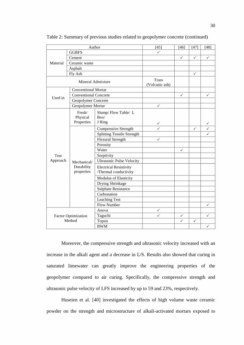
30
Table 2: Summary of previous studies related to geopolymer concrete (continued)
Author [45] [46] [47] [48]
Material
GGBFS
Cement
Ceramic waste
Asphalt
Fly Ash
Mineral Admixture Trass
(Volcanic ash)
Used in
Conventional Mortar
Conventional Concrete
Geopolymer Concrete
Geopolymer Mortar
Test
Approach
Fresh/
Physical
Properties
Slump/ Flow Table/ L
Box/
J Ring
Mechanical/
Durability
properties
Compressive Strength
Splitting Tensile Strength
Flexural Strength
Porosity
Water
Penetration/Absorption
Sorptivity
Ultrasonic Pulse Velocity
Electrical Resistivity
/Thermal conductivity
Modulus of Elasticity
Drying Shrinkage
Sulphate Resistance
Carbonation
Leaching Test
Flow Number
Factor Optimization
Method
Anova
Taguchi
Topsis
BWM
Moreover, the compressive strength and ultrasonic velocity increased with an
increase in the alkali agent and a decrease in L/S. Results also showed that curing in
saturated limewater can greatly improve the engineering properties of the
geopolymer compared to air curing. Specifically, the compressive strength and
ultrasonic pulse velocity of LFS increased by up to 59 and 23%, respectively.
Huseien et al. [40] investigated the effects of high volume waste ceramic
powder on the strength and microstructure of alkali-activated mortars exposed to

31
elevated temperatures. Concrete mixes were produced by blending the wastes from
Malaysian agro and construction industries including CWP, GGBFS, and FA. As-
prepared mortar specimens were heated up to 900°C to determine their temperature-
dependent residual compressive strength, weight loss, and microstructure. The
deterioration of alkali-activated mortar specimens was evaluated at elevated
temperatures by XRD, thermogravimetric analysis (TGA), FTIR spectroscopy, and
field emission scanning electron microscopy (FESEM). The study revealed that the
resistance of the proposed mortars to elevated temperatures was increased by
increasing the CWP content from 50 to 70%. In addition, FA replacement of GGBFS
led to a reduction of the mortar deterioration with mixes made with 70% CWP, 20%
GGBFS, and 10% FA showed the optimum resistance to elevated temperatures.
In another study [41], the effect of CWP on the performance of alkali-
activated mortars made with GGBFS and FA was examined. In this study, the ternary
blend was activated by a low concentration of an alkaline solution (4 M). CWP was
kept with a high content of 50, 60, and 70% of the total binder mass. The specimens
were cured at an ambient temperature of 27°C and tested at eight different ages.
Microstructure tests such as XRD, SEM, and FTIR were conducted to evaluate the
effect of the high content of CWP on the formulation of sodium aluminum silicate
hydrate (N-A-S-H), calcium aluminum silicate hydrate (C-A-S-H), and calcium
silicate hydrate (C-S-H) gels. Results showed that high volume CWP produced
environment-friendly alkali-activated mortars with compressive strength higher than
70 MPa at age of 28 days. The workability and setting time were enhanced with the
increase in CWP content.
El-Hassan et al. [42, 49] studied the performance of alkali-activated GGBFS
concrete with different percentages of fly ash replacement. Three separate molarities

32
of sodium hydroxide were combined with sodium silicate to enable the binding
process. Steel fibers were introduced into the alkali-activated mix in varying volume
ratios up to 3%, by volume. Binder, alkali activator, dune sand, and coarse aggregate
were proportioned and samples were cured in ambient conditions. The study revealed
that a higher fiber content and reduced slag led to less workable concrete mixes but
with improved mechanical properties. The use of up to 25% fly ash replacement
could improve the mechanical properties. The compressive strength increased
rapidly, with, on average, 72 and 78% of the 28-day compressive strength being
obtained at the age of 1 and 7 days. The study also showed that the steel fiber
additions increased the compressive strength by up to 39 and 52% for 1- and 7-day
samples.
In other work, El-Hassan et al. [43, 44] researched the performance and
microstructure of alkali-activated slag and slag-fly ash blended concrete subjected to
different 28-day curing regimes: air, intermittent water curing, and continuous water
curing. Three concrete mixes were arranged with fixed contents of slag, desert dune
sand, and aggregate and were activated by an alkaline solution consisting of sodium
silicate and sodium hydroxide. The ratio of AAS-to-slag was varied between 0.45
and 0.55. Samples were tested to assess transport and mechanical properties. The test
showed optimal results with an alkaline activator solution-to-slag ratio of 0.50. The
study concluded that intermittent water curing was found to be the most effective
method of curing, reducing porosity and sensitivity, and increasing bulk electrical
resistivity, modulus of elasticity, and compressive strength. Microstructure
characterization highlighted calcium aluminosilicate hydrate (CASH) as the
main strength-contributing reaction product.

33
2.4 Taguchi Method in Concrete
Taguchi is a fractional factorial design method that uses orthogonal arrays to
investigate a large number of variables with an optimum number of experiments.
This method can be applied to study the influence of numerous factors in a single
investigation. The signal-to-noise (S/N) ratio is typically used in analyzing the data
and predicting the optimum results.
Hadi et al. [34] used the Taguchi method to optimize the mixture proportions
of ambient-cured geopolymer concrete with GGBFS as the main binder and fly ash,
metakaolin, and silica fume as mineral additives. The authors investigated the effect
of binder content, alkaline activator to the binder content, sodium silicate to sodium
hydroxide ratio (SS/SH), and sodium hydroxide (SH) molar concentration on the
properties of geopolymer concrete. A total of nine different mixes were prepared and
the samples were tested for compressive strength. The study revealed that the highest
7-day compressive strength was 60.4 MPa and achieved at ambient curing
temperatures. Compressive strength of geopolymer concrete reduced when GGBFS
was partially replaced with fly ash, metakaolin, and silica fume.
The feasibility of the Taguchi Method’s dynamic approach to optimize alkali-
activated mortar using GGBFS and natural pozzolans was studied by Onoue and Bier
[45]. The flow and flexural and compressive strength were considered as the
response variables, while the design parameters included the binder content,
concentration of sodium hydroxide solution, GGBFS replacement ratio, mixing
regime, mixing time, curing temperature, and cumulative temperature in heat curing.
Experiments were performed using an L18 orthogonal array and the response
variables were optimized by calculating the S/N ratios. The research concluded that
34
the mortar can be used as a construction material however expansion cracks were
observed due to gypsum formation after long-term immersion in 10% sulphuric acid
solution. The optimum combination of design parameters in this study was 6 M SH
concentration, SS-to-SH of 0.75, GGBFS replacement of 30%, mixing time of 4
minutes, curing temperature of 90°C, and cumulative temperature in heat treatment
of 540°C-hour.
Şimşek and Uygunoğlu [46] used the Taguchi-based TOPSIS optimization
method to determine the optimal mixture proportions of concrete containing different
polymers. Considering thirteen factors with three control levels each, a total of
twenty-seven experiments were carried out in this study using an L27 orthogonal
array. The concrete samples were tested for thermal conductivity, compressive
strength at 3, 7, and 28 days, slump flow, water absorption, split tensile strength,
production cost, and water permeability. The optimum mix design included 1% high-
density polyethylene fiber, 5% low-density polyethylene fiber, 10% polypropylene
fiber, 10% thermoplastic elastomer, 10% dimethyl terephthalate, 5% polyethylene
terephthalate, 5% polyethylene naphthalate, 450 kg of cement, 120 kg of fly ash,
0.46 water-to-binder ratio, 1.05% superplasticizer, 0.5 fine aggregate-to-total
aggregate ratio, and 0.15 coarse aggregate-to-total aggregate ratio. The results of
such a mix included a thermal conductivity, 28-day compressive strength, slump
flow, water absorption, splitting tensile strength, production cost, and water
permeability of 0.70 W/m.K, 36.4 MPa, 14 cm, 2.46%, 2.64 MPa, $608/mm2, and
2.28 cm, respectively.
In a similar approach, the TOPSIS based Taguchi optimization method was
utilized to determine the optimal mixture proportions of high strength self-
compacting concrete in a ready mix concrete plant [47]. The performance criteria

35
identified by the author for this study are the average convective heat transfer
coefficient, the percentage of air content, the slump flow, the T50 time, the water
absorption, the compressive strength, the splitting tensile strength, and the production
cost. These performance criteria were affected by five factors such as cement dosage
(400 and 425), water-to-cementitious material ratio (0.35, 0.37, and 0.39), aggregate
mixture ratio (0.6, 0.65, and 0.7), superplasticizer content (1, 1.25 and 1.5), fly ash
content (80, 100, and 120 kg), and mixture content (100, 110, and 120 kg). The
optimum mixture levels after the Taguchi experiment was found to have an average
convective heat transfer coefficient of 14.556 W/m2.K, percentage of air content of
0.1%, slump flow of 760 cm, a T50 time of 3 seconds, water absorption of 1.7%,
compressive strength of 81.2 MPa, splitting tensile strength of 5.1 MPa, and
production cost of 50.9$/mm2.
In a recent study conducted by Sharifi et al. [48], the Taguchi optimization
method was employed to model the optimum mix design of the high-strength self-
compacting concrete. The authors chose ten different quality criteria’s such as heat
transfer coefficient, air percentage, slump flow, T50 time, absorbed water
percentage, compressive strength at 2, 7, and 28 days, splitting tensile strength at 28
days, and cost. The considered factors were the same as the study [48]. In this study,
the Best-Worst method was used to attain the overall weight of the experiment with
respect to each quality characteristic while also exploiting analysis of variance
(ANOVA) to appraise the contributing factors and optimal mixture designs. The
optimal mixture design was determined to have 425 kg of cement, water-to-
cementitious binder ratio of 0.35, coarse aggregate-to-fine aggregate ratio of 0.6, 1
kg/m3 of superplasticizer, 120 kg of fly ash, and a mixing time of 120 seconds.

36
Chapter 3: Experimental Program
3.1 Introduction
This chapter highlights the detailed experimental program carried out to
attain optimum geopolymer concrete mixture proportions. As-received materials
characteristics were first determined following standardized test procedures. Then,
the optimization was carried out by evaluating the mechanical and durability
properties of mixes designed using the Taguchi method. These properties included
density, compressive, splitting tensile and flexural strength, and modulus of
elasticity, bulk resistivity, ultrasonic pulse velocity, Los Angeles abrasion,
absorption, and sorptivity. After said evaluation, basic Taguchi, BWM, and TOPSIS
methods were employed to determine the optimum geopolymer mix made with CWP
and GGBFS.
3.2 Test Program
The test program includes three experimental stages accompanied by the
empirical analysis of the results of the experiments. Properties and characteristics of
as-received materials, including particle size distribution, chemical composition,
size, surface, shape, texture, pozzolanic activity, and mineralogy were determined in
the first stage using various techniques such as Laser diffractometer, X-ray
fluorescence (XRF), scanning electron microscope (SEM), strength activity index,
and X-ray diffraction (XRD). Physical properties of the coarse and fine aggregates
were also examined in the first stage in accordance with standardized procedures.
In phase two of the study, the Taguchi method for design of experiments was
employed to proportion different geopolymer concrete mixes. Based on the

37
conducted literature survey, it was concluded that five factors, labeled A to E, had a
predominant impact on the performance of geopolymer concrete, including binder
content, CWP replacement percentage by GGBFS, alkali-activator solution (AAS)-
to-binder ratio, SS-to-SH ratio, and SH molarity or molar concentration. Each of
these factors was varied among four levels (1-4) that were suggested based on past
geopolymer-related research. The resulting L16 orthogonal array provided 16
geopolymer concrete mixes that follow the test matrix shown in Table 3. Then, S/N
ratios were developed for each property under investigation. Conditions of “higher is
better” or “lower is better” were adopted to obtain an optimum mix for each
property.
Table 3: Experimental Test Matrix with designated factors and Levels
Run A B C D E
1 1 1 1 1 1
2 1 2 2 2 2
3 1 3 3 3 3
4 1 4 4 4 4
5 2 1 2 3 4
6 2 2 1 4 3
7 2 3 4 1 2
8 2 4 3 2 1
9 3 1 3 4 2
10 3 2 4 3 1
11 3 3 1 2 4
12 3 4 2 1 3
13 4 1 4 2 3
14 4 2 3 1 4
15 4 3 2 4 1
16 4 4 1 3 2

38
The third phase of the study utilized the Best Worst Method (BWM) and
Technique for Order Preference by Similarity to Ideal Solution (TOPSIS) based
Taguchi optimization method to determine the optimum proportions of the CWP-
GGBFS blended geopolymer concrete. Unlike basic Taguchi that employs S/N ratios
and can only provide an optimum mix for each property, these two methods utilize
multi-response optimization to obtain the optimum mix for a group of properties or
all of them.
3.3 As-Received Material Properties
Coarse and fine aggregates, CWP, GGBFS, chemical activators, and
superplasticizer were the primary materials utilized in this study. It is empirical that
their properties be evaluated prior to sample preparation based on Taguchi L16 mix
designs.
3.3.1 Binding Material
Ceramic waste powder and GGBFS were the binding materials used in this
study and their properties are explained in the below sub sections.
3.3.1.1 Ceramic Waste Powder
Exeed Industries Company located in Abu Dhabi, United Arab Emirates
supplied the CWP. Typical ceramic tiles burn the raw materials, including feldspar,
ball clay, china clay, silica, and kaolin, at 1200°C. The product is then polished to
obtain the final ceramic tile. The by-product of this polishing process is the CWP.
The as-received CWP had an average moisture content of about 36%, by mass. The
material was therefore dried in the oven at 110°C for 24 hours to remove any excess

39
moisture. The dried CWP coagulated together and formed larger particles. With
limited quantity passing the 300-µm sieve, the CWP was ground to an average size
of 5-10 µm and a specific surface area (SSA) of 5550 cm2/g. Figure 1 shows the
particle size distribution. The final i.e. dried and ground, CWP is shown in Figure 2.
It was stored in air-tight containers until use to avoid having any contact with
moisture.
Figure 1: Particle size distribution of CWP

40
Figure 2: Dried and ground ceramic waste powder
The chemical composition of CWP, given in Table 4, shows that it mainly
consists of SiO2 (68.6%) and Al2O3 (17.0%), indicating its potential use as an
aluminosilicate binder in geopolymer concrete. The microstructure of CWP is
characterized by irregular and angular particles, as shown in the micrographs of
Figure 3. The XRD spectrum presented in Figure 4 highlights the amorphous
structure of CWP with peaks of feldspar, calcite, and quartz, among others.
Table 4: Chemical composition of CWP and GGBFS
Components CWP (%) GGBFS (%)
SiO2 68.6 35.4
CaO 1.7 42.1
Al2O3 17.0 10.6
Fe2O3 0.8 0.4
MgO 2.5 8.1
SO3 0.1 0.3
LOI 1.8 3.1
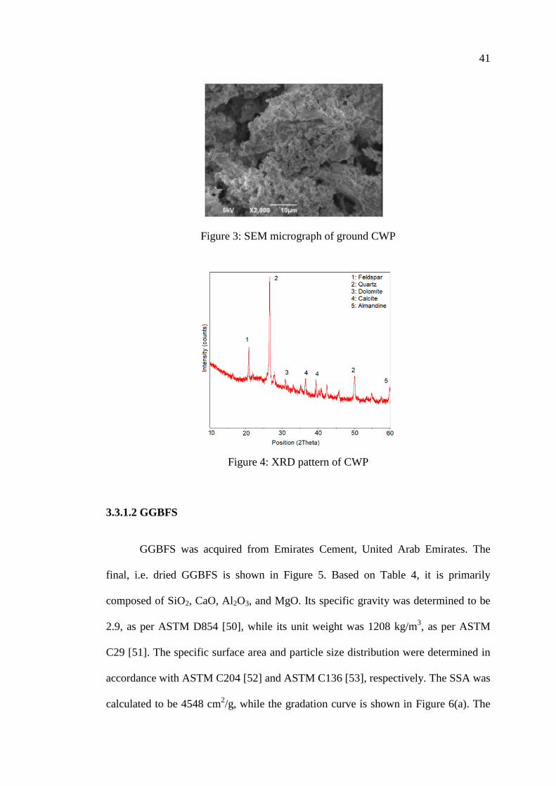
41
Figure 3: SEM micrograph of ground CWP
Figure 4: XRD pattern of CWP
3.3.1.2 GGBFS
GGBFS was acquired from Emirates Cement, United Arab Emirates. The
final, i.e. dried GGBFS is shown in Figure 5. Based on Table 4, it is primarily
composed of SiO2, CaO, Al2O3, and MgO. Its specific gravity was determined to be
2.9, as per ASTM D854 [50], while its unit weight was 1208 kg/m3, as per ASTM
C29 [51]. The specific surface area and particle size distribution were determined in
accordance with ASTM C204 [52] and ASTM C136 [53], respectively. The SSA was
calculated to be 4548 cm2/g, while the gradation curve is shown in Figure 6(a). The

42
morphology of GGBFS is that of glassy angular particles, as shown in the
micrograph of Figure 6(b). Its structure comprises quartz, mullite, and gehlenite with
an amorphous nature given the increase in the baseline of the XRD pattern between
25 and 35°2θ in Figure 6(c). Based on past literature, the use of GGBFS significantly
reduced the setting time of geopolymers but led to impressive mechanical properties
[43, 54-61].
Figure 5: As-received GGBFS
(a)
Figure 6: Particle size distribution graph (a) and SEM micrograph (b) XRD Pattern
(c) of GGBFS
0
20
40
60
80
100
1 10 100
Per
centa
ge
Pas
sing(%
)
Particle size (µm)

43
(b)
(c)
Figure 6: Particle size distribution graph (a) and SEM micrograph (b) XRD Pattern
(c) of GGBFS (continued)
3.3.2 Coarse Aggregates
Coarse aggregates in the form of crushed dolomitic limestone were utilized.
Their nominal maximum size was 19 mm. They were prepared to surface saturated
dry (SSD) conditions prior to use in the mixture. The physical properties of coarse
aggregates are shown in Table 5. Their particle size distribution, shown in Figure 7,
is within the upper and lower limits of ASTM C33 [62].

44
Figure 7: Particle size distribution graph for coarse aggregate
Table 5: Physical properties of coarse and fine aggregates
Property Unit Standard Test Coarse
Aggregate Dune Sand
Dry rodded density kg/m3 ASTM C29 [51] 1635 1660
Absorption % ASTM C127 [63] 0.22 -
Los Angeles abrasion % ASTM C131 [64] 16.0 -
Surface area cm2/g ASTM C136 [53] 2.49 116.90
Soundness (MgSO4) % ASTM C88 [65] 1.20 -
Specific gravity - ASTM C127 [63] 2.82 2.70
Fineness modulus - ASTM C136 [53] 6.82 1.45
3.3.3 Fine Aggregates
Dune sand was used as a fine aggregate. It had a specific gravity of 2.7, a unit
weight of 1660 kg/m3, and a fineness modulus of 1.45. Its specific surface area was
116.9 cm2/g. Sieve analysis was employed to determine the particle size distribution
of dune sand, as illustrated in Figure 8. The physical properties of fine aggregates are
shown in Table 5. The SEM micrograph and XRD pattern of dune sand are provided
in Figure 9 (a) and (b), respectively.
0
20
40
60
80
100
1 10 100
Cu
mu
lati
ve
Pas
sin
g (
%)
Particle Size (mm)

45
Figure 8: Particle size distribution of dune sand
(a) (b)
Figure 9: SEM (a) XRD (b) pattern for dune sand
3.3.4 Alkaline Activators
Sodium hydroxide (SH) and sodium silicate (SS) were combined to form the
alkaline activator solution. Sodium hydroxide solution was formed by mixing 98%-
pure SH flakes (Figure 10(a)) with specific amounts of water to create solutions with
different molarities, namely 8, 10, 12, and 14 M. The grade “N” sodium silicate
solution (Figure 10(b)) consisted of 26.3% SiO2, 10.3% Na2O, and 63.4% H2O.
0
20
40
60
80
100
10 100 1000
Per
cen
tage
pas
sin
g (
%)
Particle size (µm)

46
3.3.5 Superplasticizer
BASF Masterglenium Sky 504 was used as a superplasticizer. It is a
polycarboxylic ether (PCE) polymer-based superplasticizer that helps in obtaining a
high-quality concrete mix with accelerated strength development and extended
workability without delayed setting characteristics. Figure 3.10(c) shows the used
superplasticizer.
(a) (b)
(c)
Figure 10: NaOH flakes (a), Sodium silicate (b), and Superplasticizer (c)
3.4 Concrete Mixture Proportions
Selection of optimal mix using Taguchi method and the details of control
mix-C1 and C2 are given in the below subsections.
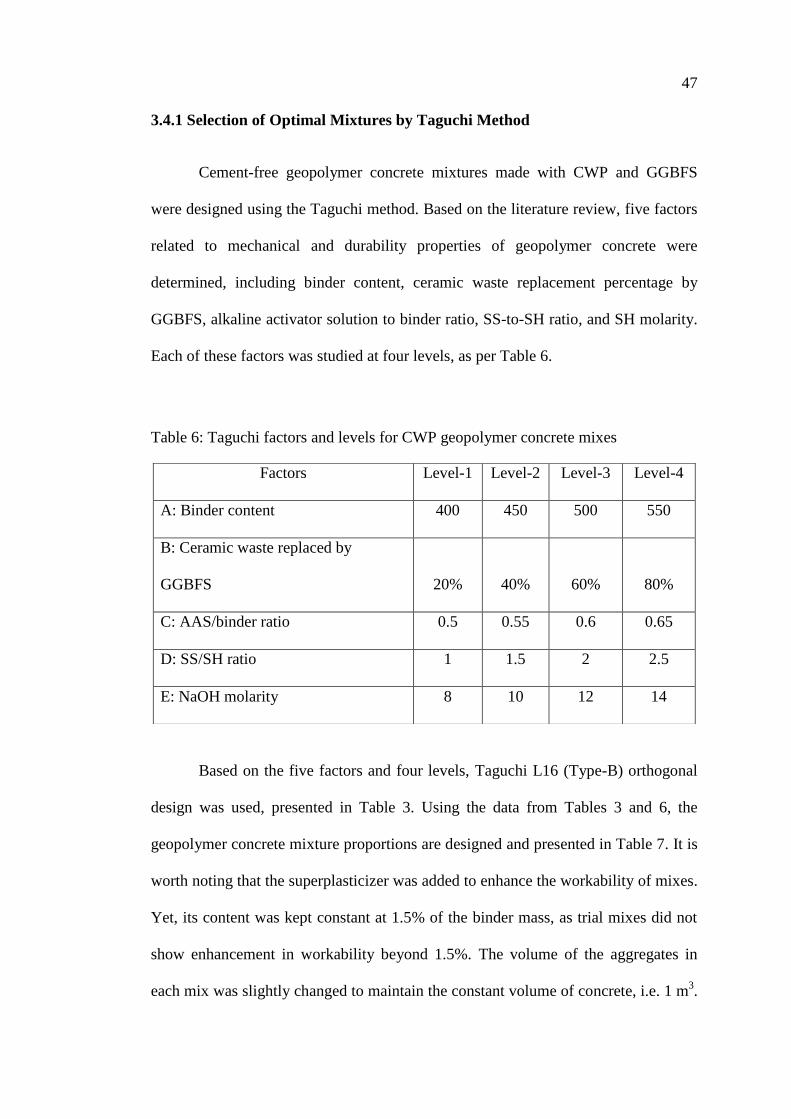
47
3.4.1 Selection of Optimal Mixtures by Taguchi Method
Cement-free geopolymer concrete mixtures made with CWP and GGBFS
were designed using the Taguchi method. Based on the literature review, five factors
related to mechanical and durability properties of geopolymer concrete were
determined, including binder content, ceramic waste replacement percentage by
GGBFS, alkaline activator solution to binder ratio, SS-to-SH ratio, and SH molarity.
Each of these factors was studied at four levels, as per Table 6.
Table 6: Taguchi factors and levels for CWP geopolymer concrete mixes
Based on the five factors and four levels, Taguchi L16 (Type-B) orthogonal
design was used, presented in Table 3. Using the data from Tables 3 and 6, the
geopolymer concrete mixture proportions are designed and presented in Table 7. It is
worth noting that the superplasticizer was added to enhance the workability of mixes.
Yet, its content was kept constant at 1.5% of the binder mass, as trial mixes did not
show enhancement in workability beyond 1.5%. The volume of the aggregates in
each mix was slightly changed to maintain the constant volume of concrete, i.e. 1 m3.
Factors Level-1 Level-2 Level-3 Level-4
A: Binder content 400 450 500 550
B: Ceramic waste replaced by
GGBFS 20% 40% 60% 80%
C: AAS/binder ratio 0.5 0.55 0.6 0.65
D: SS/SH ratio 1 1.5 2 2.5
E: NaOH molarity 8 10 12 14

48
Mixes made with 100% CWP were not considered in the L16 array, as preliminary
testing presented weak compressive strength results. Thus, a mix with 100% CWP
only served as a control. Similarly, mixes made with 100% GGBFS were not
included in the array, as they did not include CWP and were out of the scope of this
work. Yet, such mixes served as control benchmarks, denoted as C1 and C2.
Table 7: Design mixtures for Taguchi optimization of geopolymer concrete (kg/m3)
Mix
Number
Binder Aggregate Activator
SP Total CWP GGBFS Dune
Sand
Coarse
Agg. SS SH
(Molarity) T1 320 80 621 1180 100 100 (8) 6 2407
T2 240 160 605 1172 132 88 (10) 6 2403
T3 160 240 590 1171 160 80 (12) 6 2407
T4 80 320 575 1165 186 74 (14) 6 2406
T5 360 90 568 1132 165 83 (14) 7 2404
T6 270 180 586 1140 161 64 (12) 7 2408
T7 180 270 534 1122 146 146 (10) 7 2405
T8 90 360 551 1127 162 108 (8) 7 2405
T9 400 100 552 1049 214 86 (10) 8 2408
T10 300 200 550 1020 217 108 (8) 8 2403
T11 200 300 551 1095 150 100 (14) 8 2404
T12 100 400 552 1070 138 138 (12) 8 2405
T13 440 110 502 985 215 143 (12) 8 2403
T14 330 220 473 1045 165 165 (14) 8 2406
T15 220 330 495 1050 216 86 (8) 8 2406
T16 110 440 516 1055 183 92 (10) 8 2404
C1 500 0 551 1070 183 92 (14) 8 2404
C2 0 450 600 1100 161 64 (14) 8 2383
3.4.2 Control Mix C1 with 100% CWP
The mixture proportions of the control mix made with 100% CWP,
designated as C1 in Table 7, was designed based on the mix that yielded the highest
compressive strength values among the 16 mixes (T1 to T16) but without the
GGBFS. Accordingly, the control mix C1 was designed with a binder content of 500
kg/m3, AAS/binder ratio of 0.55, SS/SH ratio of 2, and SH molarity of 14. The
aggregates and superplasticizer contents were calculated similarly to other mixes.

49
3.4.3 Control Mix C2 with 100% GGBFS
Past research has utilized the same material used in this work except for the
CWP [42-44]. Thus, the mixture proportions of control mix C2 made with 100%
GGBFS were those of the mix that achieved the highest compressive strength. The
binder content of the mix was 450 kg/m3, SS/SH ratio of 2.5, SH molarity of 14,
AAS/binder of 0.5, and SP of 2.5%, by binder mass, a fine aggregate of 600 kg/m3,
and coarse aggregate of 1100 kg/m3.
3.5 Sample Preparation
The solution of sodium hydroxide was formulated 24 hours before casting.
Once it reached room temperature, it was added to sodium silicate. It was empirical
that the alkaline activator solution is prepared following this mixing procedure to
allow for the dissipation of heat associated with the chemical reactions between SH
flakes and water and SS and SH. The CWP, GGBFS, saturated surface dry (SSD)
coarse aggregates and fine aggregates were thoroughly mixed in a pan mixer for
three to five minutes under ambient temperature of 25±2°C and relative humidity of
50±5%. The prepared alkaline activator solution was then slowly added to the
mixture followed by the superplasticizer and mixed for another 3 minutes to ensure
proper homogeneity and consistency. These freshly mixed concrete mixes were cast
into 100 mm x 200 mm cylinders (diameter x height), 100 mm cubes, and 100 mm x
100 mm x 500 mm (width x height x length) prisms in two to three layers with each
layer being vibrated using a vibrating table for 10 to 15 seconds to ensure adequate
compaction. Concrete specimens were covered and left in the mold for 24 hours, then
demolded and left to cure in ambient conditions. A total of 7 cylinders, 3 prisms, and
9 cubes were cast per mix to test different properties or quality characteristics of the

50
geopolymer concrete. The details of the standard, sample size, number of samples,
and testing age are provided in Table 8 and the prepared samples were shown in
Figure 11. Details on the testing procedures are explained in the following section.
Figure 11: Geopolymer concrete mixing and sample preparation
3.6 Concrete Testing Methodology
More than 300 samples were tested to evaluate the different properties (as per
Table 8) of geopolymer concrete mixes produced in this study. Detailed descriptions
are given in the following sections. Three samples were used for each test to obtain
an average.

51
Table 8: List of quality characteristics, standards and samples used, and age of
testing
Property Standard Sample
used
Sample
Size
No. of
Samples
Testing
Age (days)
Density (Dry) ASTM C138
[66] Cube 100x100x100 9 1, 7, and 28
Compressive
Strength (f’c) ASTM C39 [67] Cylinder 100x200 3 28
Compressive
Strength (fcu)
BS EN 12390-3
[68] Cube 100x100x100 9 1, 7, and 28
Modulus of
Elasticity (Ec)
ASTM C469
[69] Cylinder
100x200
6
28
Tensile
Splitting
strength (fsp)
ASTM C496
[70]
Flexural
strength (fr) ASTM C78 [71] Prism 100x100x500 3 28
Bulk
Resistivity
ASTM C1876
[72] Cylinder 100x200 3 28
UPV ASTM C597
[73] Cube 100x100x100 3 28
Absorption ASTM C642
[74]
Disc 100x50 1 28 Sorptivity ASTM C1585
[75]
Abrasion
Resistance
ASTM C1747
[76]
3.6.1 Compressive Strength
The compressive strength was determined by applying an axial loading on
cube and cylinder specimens at a rate of 7 kN/sec according to BS EN-12390-3 [68]
and ASTM C39 [67]. The cube specimens were tested at age of 1, 7, and 28 days,
while the cylinder specimens were tested at the age of 28 days. The test setup and
tested specimens are shown in Figure 12.
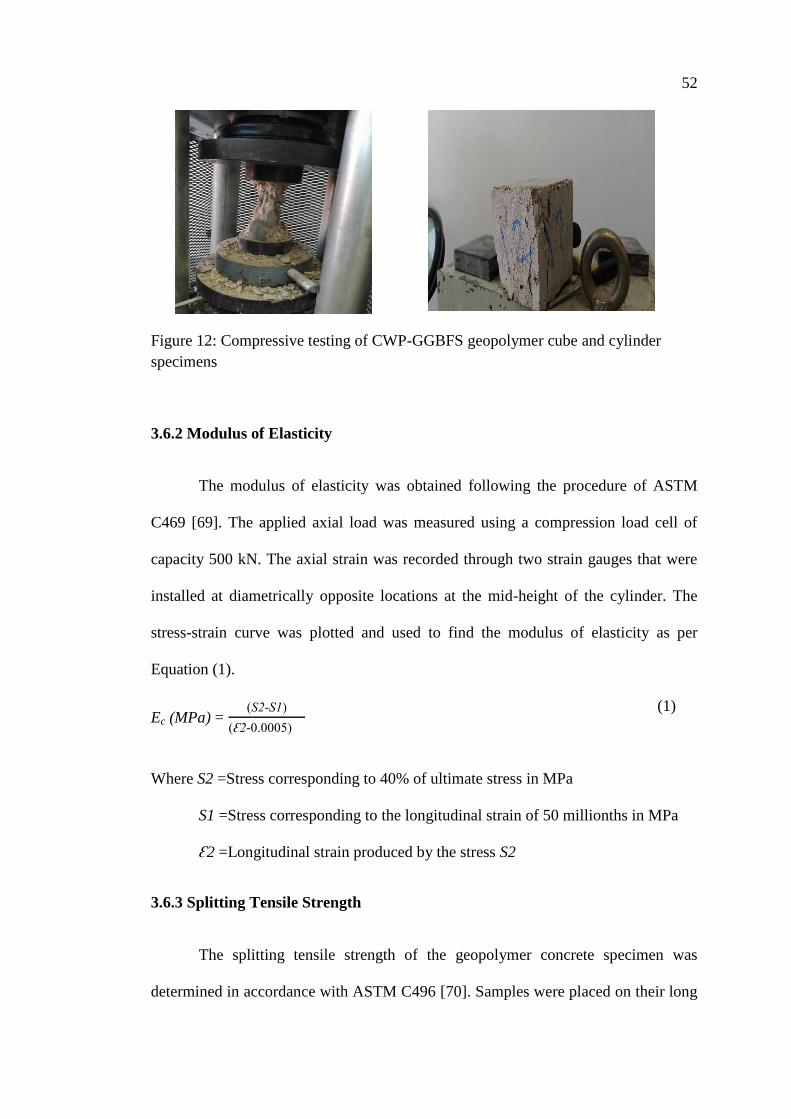
52
Figure 12: Compressive testing of CWP-GGBFS geopolymer cube and cylinder
specimens
3.6.2 Modulus of Elasticity
The modulus of elasticity was obtained following the procedure of ASTM
C469 [69]. The applied axial load was measured using a compression load cell of
capacity 500 kN. The axial strain was recorded through two strain gauges that were
installed at diametrically opposite locations at the mid-height of the cylinder. The
stress-strain curve was plotted and used to find the modulus of elasticity as per
Equation (1).
Ec (MPa) = ( - )
( - )
(1)
Where S2 =Stress corresponding to 40% of ultimate stress in MPa
S1 =Stress corresponding to the longitudinal strain of 50 millionths in MPa
2 =Longitudinal strain produced by the stress S2
3.6.3 Splitting Tensile Strength
The splitting tensile strength of the geopolymer concrete specimen was
determined in accordance with ASTM C496 [70]. Samples were placed on their long
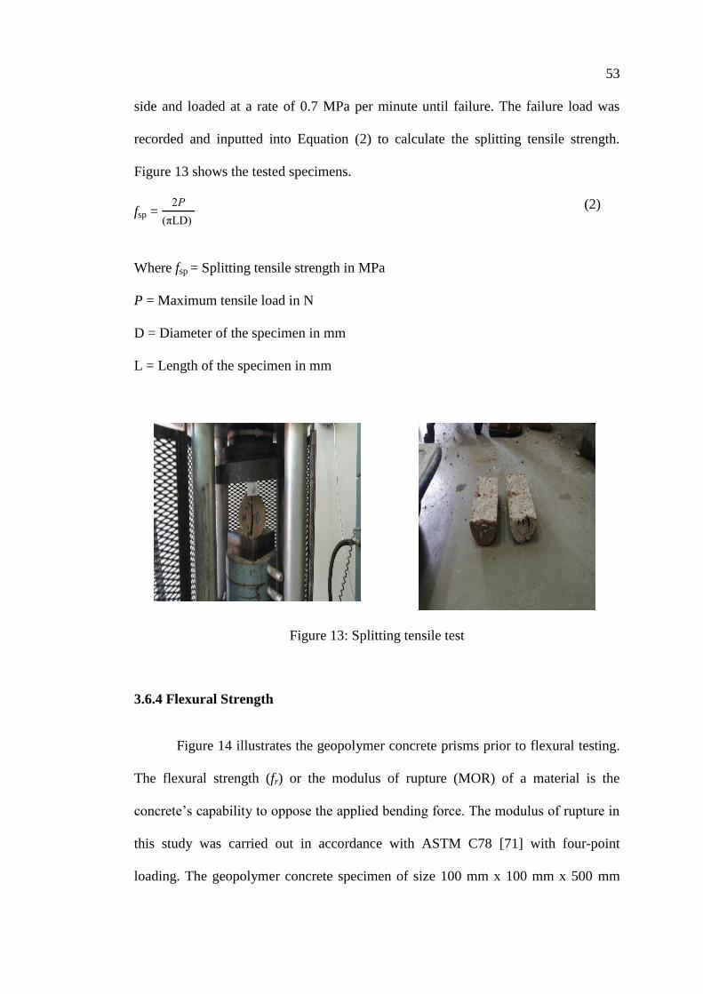
53
side and loaded at a rate of 0.7 MPa per minute until failure. The failure load was
recorded and inputted into Equation (2) to calculate the splitting tensile strength.
Figure 13 shows the tested specimens.
fsp =
( )
(2)
Where fsp = Splitting tensile strength in MPa
P = Maximum tensile load in N
D = Diameter of the specimen in mm
L = Length of the specimen in mm
Figure 13: Splitting tensile test
3.6.4 Flexural Strength
Figure 14 illustrates the geopolymer concrete prisms prior to flexural testing.
The flexural strength (fr) or the modulus of rupture (MOR) of a material is the
concrete’s capability to oppose the applied bending force The modulus of rupture in
this study was carried out in accordance with ASTM C78 [71] with four-point
loading. The geopolymer concrete specimen of size 100 mm x 100 mm x 500 mm

54
(width x height x length) was tested at the age of 28 days. A load cell was used to
record the applied load. The load was applied gradually at a rate of 1 MPa/min till
the point of failure. The flexural strength or modulus of rupture was estimated as per
Equation 3.
fr =
(bd )
(3)
Where fr = flexural strength in MPa,
P = applied load in N,
L = average specimen length in mm,
b = Average specimen width in mm,
d = Average specimen depth in mm.
Figure 14: Geopolymer concrete prism specimens prior to a flexure test
3.6.5 Bulk Resistivity
The durability of the concrete is governed by the rate of penetration of
aggressive ions. The ability of concrete to resist the diffusion of chloride or other
ions is said to be theoretically related to the bulk electrical resistivity (or bulk
resistivity). To evaluate the durability performance of geopolymer concrete made

55
with CWP and GGBFS, the bulk resistivity test was conducted in accordance with
ASTM C1876 [72] at an age of 28 days. The test setup is shown in Figure 15. The
bulk resistivity was calculated using Equation (4).
Bulk resistivity (kΩ.cm) = Applied voltage ( ) (Average sample diameter (mm))
x Current at min (mA) Average sample length in mm (4)
Figure 15: Bulk resistivity test
3.6.6 Ultrasonic Pulse Velocity
The ultrasonic pulse velocity test is a non-destructive test (NDT) that is
typically used to assess the uniformity and quality of the hardened concrete. It
generates and receives pulses of longitudinal stress waves through concrete and
measures the time it takes to cross a specific distance. The test was carried out in
accordance with ASTM C597 [73] on 100 mm geopolymer cube samples at the age
of 28 days. The pulse velocity is measured using Equation (5).
Pulse Velocity (m/s) = istance between transducers (m)
Transit time (s)
(5)

56
3.6.7 Water Absorption
The water absorption of 28-day geopolymer concrete disc specimens (100
mm x 50 mm, diameter x height) was evaluated in accordance with ASTM C642
[74]. Samples were first oven-dried at 105°C until a mass change of less than 0.5%
was reached and then immersed in water for 24 hours. They were then dried with a
towel and the saturated surface-dry mass was measured. Water absorption was
calculated using Equation (6) and the test setup is shown in Figure 16.
Water absorption (%) = SS mass (g)- ry mass (g)
ry mass (g) x
(6)
Figure 16: Water absorption test
3.6.8 Sorptivity
The sorptivity test was carried out as per ASTM C1585 [75] on similar 28-
day geopolymer concrete disc specimens to determine the rate of absorption.
Specimens were oven-dried at 105°C for 24 hours. The sides and top surface of the
disc specimens were wrapped and sealed with impermeable tape to ensure that the
water penetrates only through the bottom face while preventing water evaporation
during the test. The resulting sample was placed on a ring support in a container
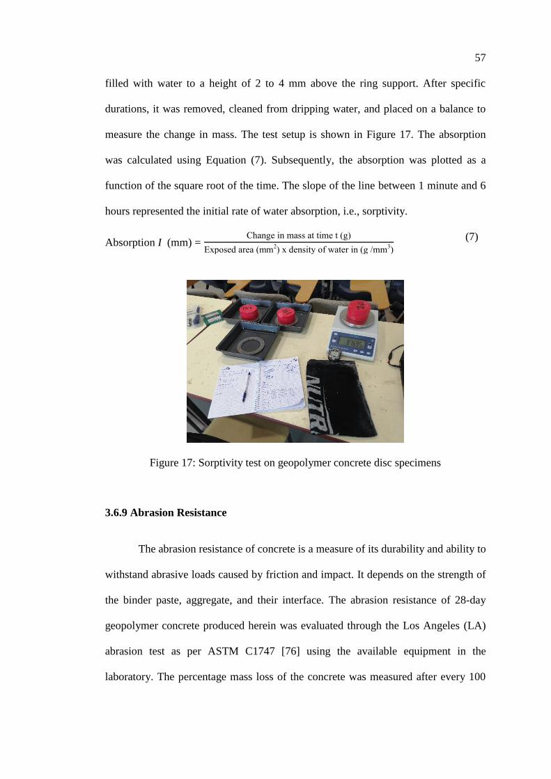
57
filled with water to a height of 2 to 4 mm above the ring support. After specific
durations, it was removed, cleaned from dripping water, and placed on a balance to
measure the change in mass. The test setup is shown in Figure 17. The absorption
was calculated using Equation (7). Subsequently, the absorption was plotted as a
function of the square root of the time. The slope of the line between 1 minute and 6
hours represented the initial rate of water absorption, i.e., sorptivity.
Absorption I (mm) = Change in mass at time t (g)
xposed area (mm ) x density of water in (g mm
) (7)
Figure 17: Sorptivity test on geopolymer concrete disc specimens
3.6.9 Abrasion Resistance
The abrasion resistance of concrete is a measure of its durability and ability to
withstand abrasive loads caused by friction and impact. It depends on the strength of
the binder paste, aggregate, and their interface. The abrasion resistance of 28-day
geopolymer concrete produced herein was evaluated through the Los Angeles (LA)
abrasion test as per ASTM C1747 [76] using the available equipment in the
laboratory. The percentage mass loss of the concrete was measured after every 100

58
revolutions for a total of 500 revolutions. A typical sample after the abrasion test is
shown in Figure 18.
(a) (b)
Figure 18: Abrasion Resistance Test (a) Weighing of specimen (b) Specimen after
500 revolutions in the LA abrasion machine
3.7 Optimization Methodology
Taguchi method can optimize the mixture proportions of any concrete,
including geopolymers, based on a single property or quality criteria. However, to
optimize all the quality criteria instantaneously and solve multi-objective problems,
the Taguchi method cannot be used [48]. Instead, multi-criteria optimization
techniques, such as Best Worst Method (BWM) and Technique for Order Preference
by Similarity to Ideal Solution (TOPSIS), have been considered to efficiently
elucidate the optimum mixture proportions for superior overall performance.
Furthermore, the results of each method can be compared by validating the
performance of its optimum mix. In this work, the steps are shown in Figure 19 and
listed as follows:
1. Identify the problem, as per Section 3.1.

59
2. Determine the control factors and levels, as per Table 6.
3. Identify the required quality criteria, as per Table 8.
4. Identify the type of test to be executed and determine the number of samples
required for the study, as per Table 8.
5. Choose a suitable orthogonal array based on the number of factors and levels.
Taguchi L16 (Type-B) Orthogonal array was chosen and given in Tables 3 and 6.
6. Conduct the experiments and obtain the test results for each quality criterion.
7. Carry out of Taguchi analysis by calculating the S/N ratio for each single quality
criteria and identify optimal values, as per Section 3.7.1.
8. Optimize mixture proportions based on the Best Worst Method, as detailed in
Section 3.7.2.
9. Optimize mixture proportions based on the TOPSIS method, as detailed in
Section 3.7.3.
10. Compare the optimal values obtained from steps 7, 8, and 9.
11. Validate the optimal values through experimental testing.

60
Figure 19: Optimization methodology proposal. Based on [46, 48].
Identify the problem Ascertain control
factors, levels and the
required quality criteria
to be considered
Identify the type of test
to be executed and
determine the number of
samples required
Select the appropriate
orthogonal array
based on chosen
number of factors
and levels
Conduct experiment
Carry out
Taguchi
Analysis
Perform Taguchi
optimization by Best worst
method (BMW) considering
all the quality criteria Perform Taguchi
optimization by
TOPSIS Method
considering all the
quality criteria 1. Calculate S/N
ratio for single
quality criteria (e.g.
compressive
strength)
2. Identify optimal
values based on the
above calculated
signal-to-noise ratio
1. Decide factors, levels and
quality criteria
2. Compute weight of each quality
criteria using BWM
3. Select orthogonal array, list out
the results, rank best experiments
with respect to each quality criteria
4. Rank worst experiments with
respect to each quality criteria
5. Compute weight of experiments
with respect to each individual
quality criteria
6. Find total weight for each
experiment with respect to all
quality criteria
7. Calculate SN ratio, determine
optimal factors and levels
1. Decision matrix computation
2. Normalization decision matrix
calculation
3. Weighted normalization
decision matrix calculation
4. Identification of positive and
negative ideal solution
5. Compute separation measures
6. Reference order Experimental
design to be ranked
7.Compute SN ratio, determine
optimal factors and levels
Analysis result from all above three method and
conclude an optimum levels for factors Validation of
optimized
experiment/mix

61
3.7.1 Taguchi Method
Professor Genichi Taguchi first introduced the Taguchi method as a design of
the experimental method in 1950 [48]. A near-optimal combination of factor levels
can be attained by this method with the least number of experiments, effectively
reducing the time and the cost of the optimization process. In order to design,
conduct, and analyze the experiments more easily and robustly and to gain
significant insight on important factors and optimal settings, Taguchi recommended
the use of orthogonal arrays in this method. These orthogonal arrays are selected
based on the number of factors and levels involved in each experiment. Results are
analyzed using the Signal to Noise (
) ratio, which is indicative of how the responses
have changed over a certain number of experiments. It also indicates the effect of
control factors on the response. The optimal control levels are therefore derived from
the setting of the control factor level with the highest
ratio value, as it minimizes
the effects of the noise factors. Different
ratio formulas, as per Equations (8-9), can
be used depending on the nature of the response.
(
) = ⌈
∑
⌉ Smaller is better (8)
(
) = ⌈
∑
⌉ Larger is better (9)
Where the test is the results for the response j of experiment i in the kth
replication and n is the total number of trial repetition.

62
3.7.2 Taguchi Optimization by Best Worst Method
This method was developed by Brunelli and Razei [68]. The authors propose
the following detailed steps to carry out this method:
1. Determine the quality criteria to be studied in the experiment.
2. Estimate the weight of each quality criteria using the BWM method based on a
comparison of best quality criteria to others and worst quality criteria to others
using a scale of 1 to 9, as per Table 9.
Table 9: Scale rate for quality criteria
Scale Meaning
1 Equal importance
2 Somewhat between Equal and Moderate
3 Moderately more important than
4 Somewhat between Moderate and Strong
5 Strongly more important than
6 Somewhat between Strong and Very strong
7 Very strongly important than
8 Somewhat between Very strong and Absolute
9 Absolutely more important than
3. The best to worst vectors AB can be represented as Equation 10.
AB= (ab1, ab2, ab3…… abn) (10)
abj indicates the preference of the best criteria b over the criteria j (1 to n)
b represents the most important criteria judged by the decision maker.
The worst to best vectors AW can be represented as Equation (11).

63
AW = (a1w, a2w, a3w…… anw) (11)
ajw indicates the preference of the criteria j over the worst criteria w (j = 1 to n).
w represents the most important criteria judged by the decision maker.
4. Reduce the absolute differences ⌊ - ⌋, ⌊ - ⌋ for all j to find the
optimal weights of a criteria. This is carried out by solving the linear equations
given in Equations (12) and (13). These equations were solved here in study by
suing BWM excel solver proposed by Brunelli and Razei [68].
⌊ - ⌋≤ ξ for all j (12)
⌊ - ⌋≤ ξ for all j (13)
where ∑
for all j
ξ is the consistency ratio
is the preference of best criteria b over the criteria j ( , ,…,n)
is the preference of criteria j over the worst criteria w
indicates the optimal weights of best, worst, and other criteria
respectively.
5. Rank the best experiments from Taguchi orthogonal array with respect to each
quality criteria using a scale 1 to 9.
6. Rank the worst experiments from Taguchi orthogonal array with respect to each
quality criteria using a scale 1 to 9
7. Estimate the weight of each experiment with respect to each quality criteria.
8. Estimate the total weight with respect to all quality criteria.
9. Estimate the signal-to-noise ratio for the total weight of the experiment. In this
step, the S/N ratio for the total weight of experiments with respect to all quality

64
criteria is calculated using the appropriate equations given in Equations (8-9).
The highest S/N ratio is chosen as the optimal design.
BWM analysis, as per above the steps, was carried out thrice with three, five,
and nine quality criteria to verify whether similar optimal designs are achieved and to
decide on whether all the quality criteria should be taken into consideration or a
fewer number is sufficient for proper optimization and analysis. Figure 20 shows the
proposed BWM model, where Q1, Q2, Q3, … are the quality characteristics and T ,
T2, T3, ... are the experiments.
Figure 20: Schematic of the BWM model
3.7.3 Taguchi Optimization by TOPSIS Method
Hwang and Yoon developed the TOPSIS method to solve multi-criteria
decision-making problems. The alternatives are categorized on the basis of the idea
of a compromise solution that would take a shorter distance from a positive ideal
solution (PIS) and the longest distance from the negative ideal solution (NIS). The
steps involved in the TOPSIS methodology, which usually converts the multi-
response problem into a single response one, are as follows:

65
1. Determine the decision matrix, D. The characteristic values of alternatives
(experiments) and attributes (calculated
ratios of responses) are arranged in a
matrix form as shown in Equation (14).
D = [
] (14)
where D is the decision matrix
is the number of experiments,
i = , , … the number of experiments m and j = , , … the number of responses n
2. Compute the normal ratings by vector normalisation ( )using Equation (15).
= -
√∑
where i = , ,… m and j = , ,…n (15)
3. Compute the weighted normalised decision matrix. The normalisation values of
each response are multiplied by the corresponding weight value. The same
weight values estimated in step 2 of BWM method were used for this purpose.
Weighted normalised decision matrix (V) was then determined using equation
Equation (16).
V=[ ] (16)
where = ,
and ∑ =1
4. Calculate the positive ideal solution (PIS=A+) and the negative ideal solution
(NIS=A-) using Equations (17) and (18).
A+ = (
, ……,
) where =max (17)
A- = ( -
-,
-……,
-) where
-=min (18)
66
5. The separation measures of alternative (experiment number) i to the positive
ideal solution (Si+) and the distance from the negative ideal solution (Si-) were
estimated using Equations (19) and (20).
Si+ = √∑ ( - ) (19)
Si- = √∑ ( - -) (20)
6. Rank the Reference order Experimental design by calculating the ranking score
Ci* using Equation (21).
Ci* =
-
(21)
7. Calculate the S/N ratio corresponding to all experiments using Equation (9). The
combination with the highest S/N ratio is chosen as the optimal design.
Similar to the BWM method, TOPSIS analysis was carried out, as per the
above steps, thrice with three, five, and nine quality criteria.

67
Chapter 4: Results and Discussion
4.1 Introduction
The main aim of this study is to utilize multiple optimization techniques,
including Taguchi, BWM, and TOPSIS, to attain an optimized geopolymer concrete
mix made with CWP and GGBFS with superior mechanical and durability
properties. To this extent, geopolymer concrete mixture proportions were varied
based on a Taguchi L16 orthogonal array with 5 factors and 4 levels. The
experimental test results comprise density, compressive, splitting tensile and flexural
strength, modulus of elasticity, water absorption, sorptivity, bulk resistivity, UPV,
and abrasion resistance. Yet, it should be noted that mixes T12 and T14 could not be
cast due to rapid hardening and limited workability, possibly due to the use of higher
binder content of 500-550 kg/m3 in conjunction with a low SS/SH ratio of 1. Further,
the potential use of CWP as a binder in geopolymer concrete production is explored
in this chapter.
4.2 Experimental Results
All the obtained experimental results are analysed and explained in the below
subsections.
4.2.1 Fresh and Hardened Geopolymer Concrete Density
Table 10 summarizes the values of fresh and 28-day hardened density of
geopolymer concrete. Since the densities follow a similar trend, the focus will be on
the latter. The values ranged from 2302 to 2486 kg/m3, which were within the range
of normal-weight cement-based concrete mixtures. Mix T11 gave the highest
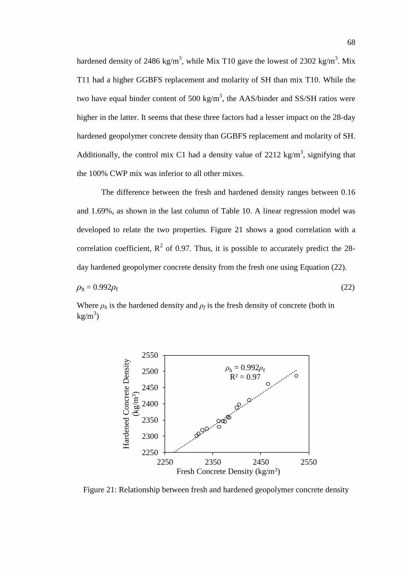
68
hardened density of 2486 kg/m3, while Mix T10 gave the lowest of 2302 kg/m
3. Mix
T11 had a higher GGBFS replacement and molarity of SH than mix T10. While the
two have equal binder content of 500 kg/m3, the AAS/binder and SS/SH ratios were
higher in the latter. It seems that these three factors had a lesser impact on the 28-day
hardened geopolymer concrete density than GGBFS replacement and molarity of SH.
Additionally, the control mix C1 had a density value of 2212 kg/m3, signifying that
the 100% CWP mix was inferior to all other mixes.
The difference between the fresh and hardened density ranges between 0.16
and 1.69%, as shown in the last column of Table 10. A linear regression model was
developed to relate the two properties. Figure 21 shows a good correlation with a
correlation coefficient, R2 of 0.97. Thus, it is possible to accurately predict the 28-
day hardened geopolymer concrete density from the fresh one using Equation (22).
ρh = 0.992ρf (22)
Where ρh is the hardened density and ρf is the fresh density of concrete (both in
kg/m3)
Figure 21: Relationship between fresh and hardened geopolymer concrete density
ρh = 0.992ρf
R² = 0.97
2250
2300
2350
2400
2450
2500
2550
2250 2350 2450 2550
Har
den
ed C
oncr
ete
Den
sity
(kg/m
3)
Fresh Concrete Density (kg/m3)

69
Table 10: Fresh and hardened density of geopolymer concrete
Mixture
Designation
Fresh
Density
(kg/m3)
Hardened
Density
(kg/m3)
Difference between
fresh and hardened
density (%)
T1 2328 2319 0.39
T2 2426 2411 0.62
T3 2371 2346 1.05
T4 2362 2347 0.64
T5 2400 2388 0.50
T6 2384 2357 1.13
T7 2381 2360 0.88
T8 2405 2398 0.29
T9 2337 2323 0.60
T10 2316 2302 0.60
T11 2524 2486 1.51
T13 2320 2308 0.52
T15 2363 2329 1.44
T16 2465 2461 0.16
C1 2250 2212 1.69
C2 2475 2445 1.21
4.2.2 Water Absorption and Sorptivity
Table 11 presents the water absorption of hardened geopolymer concrete.
Based on the results, mixes T11, T16, T2, and T8 have the lowest absorption values,
ranging from 4.15 to 4.53%. Of these mixes, none had a GGBFS replacement below
40%, AAS/binder ratio above 0.6, SS/SH ratio above 2, or SH molarity of 12.
Conversely, mixes T10 and C1 showed the highest absorption of 7.02 and 8.35%,
nearly 69 and 101% larger than that of mix T11, respectively. Clearly, higher
AAS/binder (>0.6) and SS/SH (>2) led to a less dense mix with more pore space, and
consequently, higher water absorption. Also, the incorporation of GGBFS into CWP

70
geopolymer mixes seems critical to obtaining a dense matrix. In fact, 100% GGBFS
mix (C2) had the second-lowest absorption of 4.23%.
The rate of water absorption, i.e. sorptivity, is a measure of geopolymer
concrete’s ability to transport water into its matrix through capillary suction.
Although two forms of sorptivity are typically measured, namely initial and
secondary, past research on geopolymer concrete proved that the former is much
larger than the latter [43]. This is because the former is associated with the sorption
process by the capillary pores while the latter corresponds to the sorption by the gel
pores [78]. Therefore, the focus of this work is on the initial sorptivity.
Table 11: Water absorption and initial rate of water absorption of CWPGC
Mixture Water Initial rate of
Designation absorption
(%)
absorption
(mm √s)
T1 6.31 0.038
T2 4.38 0.028
T3 5.75 0.038
T4 5.71 0.037
T5 4.73 0.027
T6 4.88 0.027
T7 4.98 0.037
T8 4.53 0.029
T9 6.57 0.045
T10 7.02 0.047
T11 4.15 0.027
T13 6.83 0.05
T15 6.1 0.047
T16 4.29 0.028
C1 8.35 0.055
C2 4.23 0.029

71
(a) (b)
(c) (d)
(e)
Figure 22: Development of absorption with time for mixes with CWP-to-GGBFS
ratio of (a) 4:1 (b) 3:2 (c) 2:3 (d) 1:4 and (e) control mixes
Sorptivity test results are presented in the form of absorption over time, as
shown in Figure 22(a-e). Mixes were grouped by GGBFS replacement percentages
20, 40, 60, and 80%. For these groups, the lowest sorptivity values were in the range
of 0.027-0.028 mm/s0.5
for mixes T5, T6, T11, and T16, respectively. Such mixes are
characterized by AAS/binder ratios below 0.6 and SH molarity of 10 and above. In
0
1
2
3
4
5
6
7
8
9
10
0 25 50 75 100 125 150 175
I (m
m)
Time (√s)
T1 T5
T9 T13
0
1
2
3
4
5
6
7
8
9
10
0 25 50 75 100 125 150 175
I (m
m)
Time (√s)
T2 T6
T10
0
1
2
3
4
5
6
7
8
9
10
0 25 50 75 100 125 150 175
I (m
m)
Time (√s)
T3 T7
T11 T15
0
1
2
3
4
5
6
7
8
9
10
0 25 50 75 100 125 150 175
I (m
m)
Time (√s)
T4 T8
T16
0
1
2
3
4
5
6
7
8
9
10
0 25 50 75 100 125 150 175
I (m
m)
Time (√s)
C2
C1
72
contrast, the highest sorptivity values were for mixes T13, T10, T15, and T4,
respectively. Their sorptivity ranged between 0.037 and 0.052 mm/s0.5
, representing
values that were, on average, 71% higher than the lowest ones. Yet, it is worth noting
that this increase in sorptivity was more apparent at lower GGBFS replacement
percentages.
4.2.3 Compressive Strength
Figure 23 presents the compressive strength of the geopolymer mixes at the
ages of 1, 7, and 28 days. The mixes were grouped based on GGBFS replacement
percentages of 20, 40, 60, and 80%. The two control mixes were each in a group of
their own. Mixes T5, T2, T11, and T16 exhibited the highest compressive strength
within each group with values of 53.7, 61.5, 78.5, and 64.0 MPa, respectively. In
addition to altering the GGBFS replacement percentage, each of these mixes had a
different binder content, signifying that it may not be a major component to
obtaining high cube compressive strength (>50 MPa). On the other hand, the
AAS/binder ratio, SS/SH ratio, and SH molarity were found to be in the respective
ranges of 0.50-0.55, 1.5-2, and 10-14. Apparently, geopolymer mixes with
proportions falling beyond these ranges had inferior compressive strength, owing to
lower density and higher pore space, as evidenced by results of sections 4.2.1 and
4.2.2. Conversely, control mixes made with 100% slag or 100% CWP (C2 and C1)
had compressive strengths of 75.1 and 8.1 MPa, respectively. While C2 has a
strength higher than most mixes, except for T11, it is worth noting that eight mixes
utilizing a blend of CWP and GGBFS could attain a compressive strength above 40
MPa, which is sufficient for most structural applications. In addition, these
geopolymer concrete mixes do not require curing through heat treatment, which is

73
typically required in fly ash-based geopolymer concrete [79]. Further, unlike slag-
based geopolymers, where an SS-to-SH ratio of 2.5 led to superior strength [80, 81],
CWP-GGBFS blended geopolymers experience high compressive strength with a
ratio of 2 and less.
The cube compressive strength development profile during subsequent curing
is evaluated through the percent increase in strength from 1 to 7 days, 7 to 28 days,
and 1 to 28 days. Table 12 summarizes the results. The increase in compressive
strength from 1 to 7 days was in the range of 23 to 220%. Such variation is owed
primarily to the changes in the mixture proportions [72]. The highest three increases
were associated with mixes that had a 1-day cube compressive strength below 10
MPa. Such mixes were proportioned with a binder content of 500-550 kg/m3,
AAS/binder ratio of 0.60-0.65, and 20-40% GGBFS replacement percentage.
Apparently, the high binder content did not guarantee superior strength. Also, an
increase in the AAS/binder ratio played a similar role to a high water-to-cement ratio
in conventional concrete in that it reduced the compressive strength. Further, to attain
a 1-day compressive strength beyond 16 MPa, at least 40% GGBFS should be
incorporated into the geopolymer concrete mix. In comparison, control mix C2
experienced a 23% increase over 7 days of curing due to its high early-age
compressive strength. Actually, it presented the highest 1-day strength among all
mixes. Conversely, control mix C1 with 100% CWP did not have a 1-day
compressive strength, as the samples required three days of in-mold curing prior to
demolding and testing.
The increase in cube compressive strength from 7 to 28 days is also shown in
Table 12. Values ranged between 1 to 74%, with the highest increases noted for
mixes replacing 20% CWP with GGBFS. Similarly, the increase from 1 to 28 days

74
was highest for these samples. In comparison, control mix C2 was among those with
the lowest percent increase, owing to an accelerated geopolymerization reaction
within the first days. Also, control mix C2 had a relatively low increase from 7 to 28
days, because of the possible limited degree of reaction with CWP being the sole
binder. It can be thus concluded that early and late strength increases are dependent
on the AAS/binder ratio and GGBFS replacement percentage. The remaining factors
seem to be less impactful on the strength development.
Table 12: Compressive strength of geopolymer concrete cylinders and cubes
Mixture
Designation
Cube Compressive
Strength (MPa)
Increase in fcu
(%) Cylinder
Compressive Strength
at 28 days
(MPa) f’c/fcu
1
Day
7
Day
28
Day
1 to 7
day
7 to 28
day
1 to 28
day
T1 11.9 16.4 26.4 37.8 61.0 121.8 21.6 0.82
T2 35.3 60.5 61.5 71.4 1.7 74.2 38.5 0.63
T3 30.6 37.3 39.0 21.9 4.6 27.5 30.8 0.79
T4 23.6 34.2 40.3 44.9 17.8 70.8 31.0 0.77
T5 16.1 35.0 53.7 117.4 53.4 233.5 34.8 0.65
T6 21.1 43.1 46.7 104.3 8.4 121.3 32.7 0.70
T7 37.0 42.0 44.6 13.5 6.2 20.5 32.1 0.72
T8 42.2 52.2 55.3 23.7 5.9 31.0 37.3 0.67
T9 5.5 17.6 25.5 220.0 44.9 363.6 16.0 0.63
T10 7.6 22.0 22.8 189.5 3.6 200.0 10.6 0.46
T11 39.8 55.7 78.5 39.9 40.9 97.2 56.6 0.72
T13 4.9 13.5 23.5 175.5 74.1 379.6 13.3 0.57
T15 15.6 25.3 26.3 62.2 4.0 68.6 19.1 0.73
T16 26.4 60.9 64.0 130.7 5.1 142.4 40.9 0.64
C1 0.0 7.5 8.1 - 8.0 - 3.3 0.41
C2 59.8 73.6 75.1 23.1 2.0 25.6 54.5 0.73

75
Figure 23: Compressive strength development of CWPGC with different ceramic
percentages
Table 12 summarizes the 28-day cylinder compressive strength test results.
Values ranged from 3.3 to 56.6 MPa and the strength trend was similar to that of the
cube samples. The ratio of the cylinder to cube compressive strength is also
presented in Table 12. It falls between 0.41 and 0.82. Further, a linear regression
model is developed to relate the two compressive strength results. A strong
correlation (R2 = 0.96) existed, as shown in Figure 24. Accordingly, the 28-day
cylinder compressive strength can be predicted from the cube strength with high
accuracy using the relationship presented in Equation (23).
f’c = 0.69fcu (23)
0
10
20
30
40
50
60
70
80
90
T1 T5 T9 T13 T2 T6 T10 T3 T7 T11 T15 T4 T8 T16 C1 C2
20% 40% 60% 80% 0% 100%
Cub
e C
om
pre
ssiv
e S
tren
gth
, fc
u (
MP
a)
Mix Designation with GGBFS Replacement Percentage
1-day7-day28-day
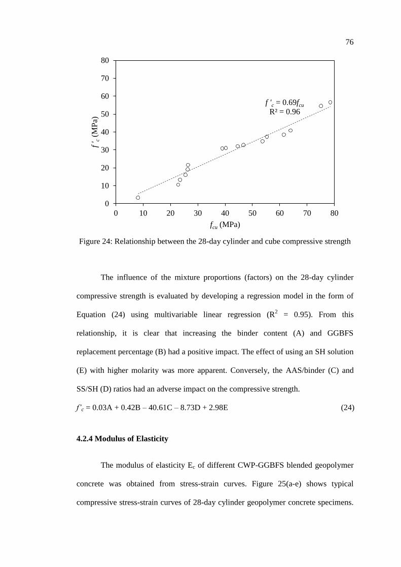
76
Figure 24: Relationship between the 28-day cylinder and cube compressive strength
The influence of the mixture proportions (factors) on the 28-day cylinder
compressive strength is evaluated by developing a regression model in the form of
Equation (24) using multivariable linear regression (R2 = 0.95). From this
relationship, it is clear that increasing the binder content (A) and GGBFS
replacement percentage (B) had a positive impact. The effect of using an SH solution
(E) with higher molarity was more apparent. Conversely, the AAS/binder (C) and
SS/SH (D) ratios had an adverse impact on the compressive strength.
f’c = 0.03A + 0.42B – 40.61C – 8.73D + 2.98E (24)
4.2.4 Modulus of Elasticity
The modulus of elasticity Ec of different CWP-GGBFS blended geopolymer
concrete was obtained from stress-strain curves. Figure 25(a-e) shows typical
compressive stress-strain curves of 28-day cylinder geopolymer concrete specimens.
f 'c = 0.69fcu
R² = 0.96
0
10
20
30
40
50
60
70
80
0 10 20 30 40 50 60 70 80
f ' c
(M
Pa)
fcu (MPa)
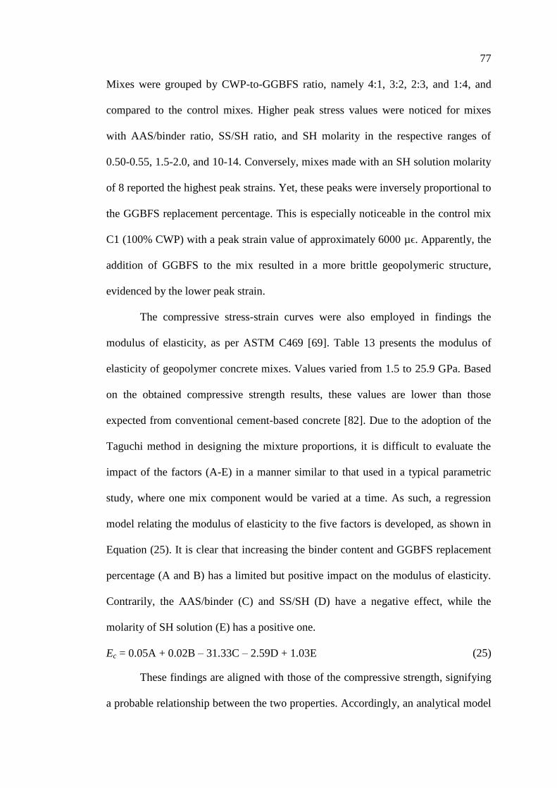
77
Mixes were grouped by CWP-to-GGBFS ratio, namely 4:1, 3:2, 2:3, and 1:4, and
compared to the control mixes. Higher peak stress values were noticed for mixes
with AAS/binder ratio, SS/SH ratio, and SH molarity in the respective ranges of
0.50-0.55, 1.5-2.0, and 10-14. Conversely, mixes made with an SH solution molarity
of 8 reported the highest peak strains. Yet, these peaks were inversely proportional to
the GGBFS replacement percentage. This is especially noticeable in the control mix
C1 (100% CWP) with a peak strain value of approximately 6000 µϵ. Apparently, the
addition of GGBFS to the mix resulted in a more brittle geopolymeric structure,
evidenced by the lower peak strain.
The compressive stress-strain curves were also employed in findings the
modulus of elasticity, as per ASTM C469 [69]. Table 13 presents the modulus of
elasticity of geopolymer concrete mixes. Values varied from 1.5 to 25.9 GPa. Based
on the obtained compressive strength results, these values are lower than those
expected from conventional cement-based concrete [82]. Due to the adoption of the
Taguchi method in designing the mixture proportions, it is difficult to evaluate the
impact of the factors (A-E) in a manner similar to that used in a typical parametric
study, where one mix component would be varied at a time. As such, a regression
model relating the modulus of elasticity to the five factors is developed, as shown in
Equation (25). It is clear that increasing the binder content and GGBFS replacement
percentage (A and B) has a limited but positive impact on the modulus of elasticity.
Contrarily, the AAS/binder (C) and SS/SH (D) have a negative effect, while the
molarity of SH solution (E) has a positive one.
Ec = 0.05A + 0.02B – 31.33C – 2.59D + 1.03E (25)
These findings are aligned with those of the compressive strength, signifying
a probable relationship between the two properties. Accordingly, an analytical model
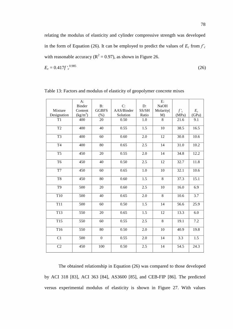
78
relating the modulus of elasticity and cylinder compressive strength was developed
in the form of Equation (26). It can be employed to predict the values of Ec from f’c
with reasonable accuracy (R2 = 0.97), as shown in Figure 26.
Ec = 0.417f 'c0.985 (26)
Table 13: Factors and modulus of elasticity of geopolymer concrete mixes
Mixture
Designation
A:
Binder
Content
(kg/m3)
B:
GGBFS
(%)
C:
AAS/Binder
Solution
D:
SS/SH
Ratio
E:
NaOH
Molarity(
M)
f 'c
(MPa)
Ec
(GPa)
T1 400 20 0.50 1.0 8 21.6 9.1
T2 400 40 0.55 1.5 10 38.5 16.5
T3 400 60 0.60 2.0 12 30.8 10.6
T4 400 80 0.65 2.5 14 31.0 10.2
T5 450 20 0.55 2.0 14 34.8 12.2
T6 450 40 0.50 2.5 12 32.7 11.8
T7 450 60 0.65 1.0 10 32.1 10.6
T8 450 80 0.60 1.5 8 37.3 15.1
T9 500 20 0.60 2.5 10 16.0 6.9
T10 500 40 0.65 2.0 8 10.6 3.7
T11 500 60 0.50 1.5 14 56.6 25.9
T13 550 20 0.65 1.5 12 13.3 6.0
T15 550 60 0.55 2.5 8 19.1 7.2
T16 550 80 0.50 2.0 10 40.9 19.8
C1 500 0 0.55 2.0 14 3.3 1.5
C2 450 100 0.50 2.5 14 54.5 24.3
The obtained relationship in Equation (26) was compared to those developed
by ACI 318 [83], ACI 363 [84], AS3600 [85], and CEB-FIP [86]. The predicted
versus experimental modulus of elasticity is shown in Figure 27. With values

79
converging around the 45°-line, it is clear that the models developed in this work, i.e.
Equation (25) and (26), were most suitable to predict the modulus of elasticity with
acceptable accuracy. Conversely, the models proposed by ACI 318 [83], ACI 363
[84], and CEB-FIP [86] tended to overestimate Ec. Nevertheless, the equation given
by AS3600 [85] slightly overestimated the values of Ec when below 16 GPa, after
which the accuracy improved. It could be thus concluded that the codified equations
may not be suitable for predicting the modulus of elasticity of geopolymer concrete
made with CWP and GGBFS unless some modification was applied.
4.2.5 Splitting Tensile Strength
The splitting tensile strength of 28-day geopolymer concrete is shown in
Table 14. Values ranged from 0.64 to 3.09 MPa with the lowest and highest being
associated with mixes C1 and T11, respectively. The trend noted for splitting tensile
strength is similar to that reported for 28-day cylinder compressive strength. As such,
an analytical model to correlate the two properties was developed, as per Figure 28
and Equation (27). It could be used to predict the splitting tensile strength from the
cylinder compressive strength with good accuracy (R2 = 0.93). Another regression
model was also established to relate fsp to the mixture proportions characterized by
the factors A-E. Equation (28) highlights this relationship. It seems that the factors
were proportional to fsp, except for the molarity of the SH solution, which was
inversely proportional.

80
Figure 25: Typical stress-strain curves of geopolymer concrete mixes with CWP-to-
GGBFS ratio of (a) 4:1 (b) 3:2 (c) 2:3 (d) 1:4 and (e) control mixes
(a) (b)
(c) (d)
(e)
0
10
20
30
40
50
60
70
0 1000 2000 3000 4000 5000 6000
Com
pre
ssiv
e S
tres
s (M
Pa)
Strain (µϵ)
T1
T5
T9
T13
0
10
20
30
40
50
60
70
0 1000 2000 3000 4000 5000 6000
Com
pre
ssiv
e S
tres
s (M
Pa)
Strain (µϵ)
T2
T6
T10
0
10
20
30
40
50
60
70
0 1000 2000 3000 4000 5000 6000
Com
pre
ssiv
e S
tres
s (M
Pa)
Strain (µϵ)
T3
T7
T11
T15
0
10
20
30
40
50
60
70
0 1000 2000 3000 4000 5000 6000
Com
pre
ssiv
e S
tres
s (M
Pa)
Strain (µϵ)
T4
T8
T16
0
10
20
30
40
50
60
70
0 1000 2000 3000 4000 5000 6000
Com
pre
ssiv
e S
tres
s (M
Pa)
Strain (µϵ)
C1
C2

81
Figure 26: Relationship between modulus of elasticity and compressive strength of
28-day geopolymer concrete
Figure 27: Predicted versus experimental values of Ec
Ec = 0.4173f 'c0.9853
R² = 0.97
0
5
10
15
20
25
30
0 10 20 30 40 50 60
Ec
(GP
a)
f'c (MPa)
0
5
10
15
20
25
30
0 5 10 15 20 25 30
Pre
dic
ted E
c (G
Pa)
Experimental Ec (GPa)
ACI 318
ACI 363
AS 3600
CEB-FIB
Equation 25
Equation 26

82
fsp = 0.4276√f
(27)
fsp = 0.001A + 0.021B + 0.063C – 0.444D + 0.134E (28)
Further, the accuracy of these two models was compared to those of codified
equations of ACI 318 [83], ACI 363 [84], AS3600 [85], and CEB-FIP [86]. Figure
29 plots the predicted versus experimental splitting tensile strength of geopolymer
concrete. Results showed that equations of ACI 318 [83] and ACI 363 [84] tended to
overestimate fsp, while those of AS3600 [85] and CEB-FIP [86] underestimated it.
However, as all these models correlate fsp to the square root of f’c, it is possible to
introduce a factor, denoted by α, that may render them more accurate For instance,
the value of α for ACI 318 [83] is noted as 0.76.
The ratio between the compressive strength and splitting tensile strength was
also calculated and is presented in the last column of Table 14. It can be noticed that
the value of fsp/f’c decreased as f’c increased. Evidently, the changes to the mixture
proportions were more impactful on f’c than on fsp. For instance, mix T11 had a 162%
higher compressive strength than mix T1, while the splitting tensile strength was
only 80% higher. This shows that the splitting tensile strength can be enhanced to a
limited extent by modifying the mixture proportions. Yet, higher values could be
achieved with the addition of steel fibers, as reported in other work [42].
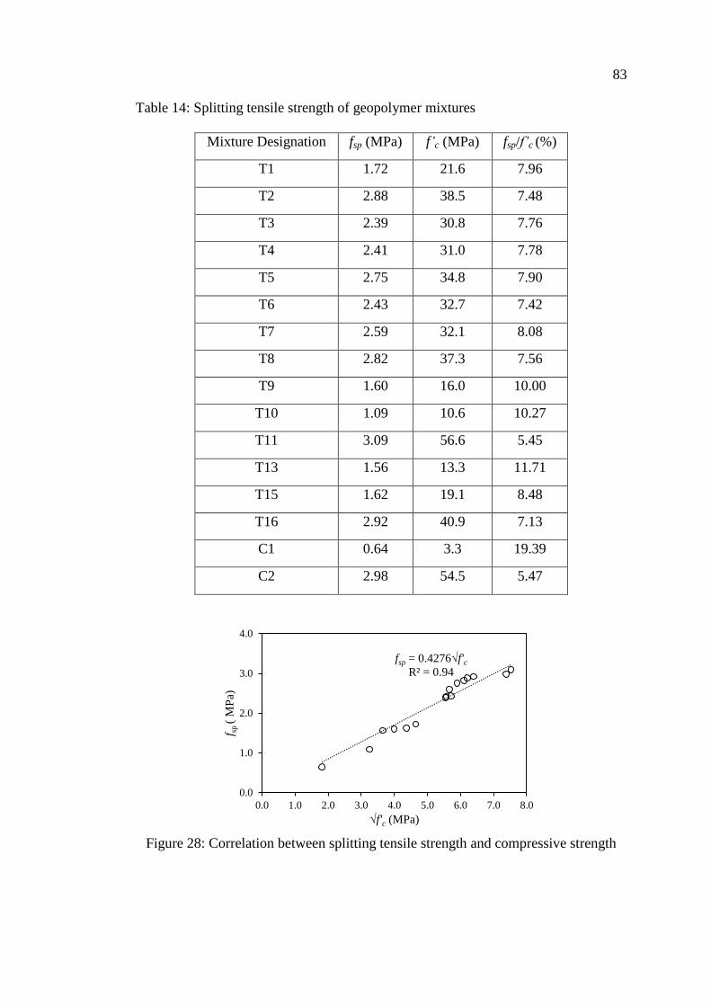
83
Table 14: Splitting tensile strength of geopolymer mixtures
Mixture Designation fsp (MPa) f’c (MPa) fsp/f’c (%)
T1 1.72 21.6 7.96
T2 2.88 38.5 7.48
T3 2.39 30.8 7.76
T4 2.41 31.0 7.78
T5 2.75 34.8 7.90
T6 2.43 32.7 7.42
T7 2.59 32.1 8.08
T8 2.82 37.3 7.56
T9 1.60 16.0 10.00
T10 1.09 10.6 10.27
T11 3.09 56.6 5.45
T13 1.56 13.3 11.71
T15 1.62 19.1 8.48
T16 2.92 40.9 7.13
C1 0.64 3.3 19.39
C2 2.98 54.5 5.47
Figure 28: Correlation between splitting tensile strength and compressive strength
fsp = 0.4276√f'c
R² = 0.94
0.0
1.0
2.0
3.0
4.0
0.0 1.0 2.0 3.0 4.0 5.0 6.0 7.0 8.0
f sp
( M
Pa)
√f'c (MPa)

84
Figure 29: Predicted and experimental splitting tensile strength
4.2.6 Flexural Strength
The flexural strength results of 28-day ambient-cured geopolymer concrete
are given in Table 15. The highest and lowest fr values were 4.87 and 0.8 MPa for
mix T11 and C1, respectively. A more in-depth analysis of the results shows that to
maximize flexural strength, a minimum SH molarity of 10, SS/SH of 1.5, and
AAS/binder of 0.50-0.55 should be adopted in the mixture proportions. The GGBFS
replacement and binder content seem to have a less apparent influence on the flexural
strength. Table 15 also presents the ratio of flexural strength to compressive strength.
Values ranged from 8 to 24% with smaller values being associated with mixes with
higher compressive strength. Accordingly and similar to the splitting tensile strength
results, the ratio is inversely proportional to f’c, signifying that variations in mixture
proportions are more impactful on f’c rather than fr. For example, f’c of mix T11 is
162% higher than that of mix T1, while fr is only 85% higher.
0.0
0.5
1.0
1.5
2.0
2.5
3.0
3.5
4.0
4.5
5.0
0.0 0.5 1.0 1.5 2.0 2.5 3.0 3.5 4.0 4.5 5.0
Pre
dic
ted
fsp
(M
Pa)
Experimental fsp (MPa)
ACI 318
ACI 363
AS3600
CEB-FIB
Equation 27
Equation 28

85
Table 15: Flexural strength of geopolymer concrete
Mixture Designation
Designation
fr (MPa) f’c (MPa) fr/f’c (%)
T1 2.64 21.6 12.24
T2 4.47 38.5 11.61
T3 3.37 30.8 10.95
T4 3.43 31.0 11.06
T5 3.98 34.8 11.44
T6 3.70 32.7 11.32
T7 3.48 32.1 10.84
T8 4.45 37.3 11.93
T9 2.31 16.0 14.44
T10 1.64 10.6 15.47
T11 4.87 56.6 8.61
T13 1.97 13.3 14.79
T15 2.39 19.1 12.51
T16 4.47 40.9 10.93
C1 0.80 3.3 24.24
C2 4.65 54.5 8.53
A comparison between the findings of f’c and fr shows that the two properties
follow similar trends. As such, linear regression analysis was utilized to develop a
model to correlate f’c and fr. The relationship, in the form of Equation (29) and
shown in Figure 30, could be employed to predict the flexural strength from the
cylinder compressive strength with good accuracy (R2 = 0.93). Another multivariable
regression model was developed (Equation 30) to relate the mixture proportions
(factors A-E) to fr. Higher AAS/binder (C) and SS/SH (D) seem to have a negative
impact on the flexural strength, while the molarity of SH solution (E) had a positive
one. Conversely, increasing the binder content (A) and GGBFS replacement
percentage (B) could result in a limited increase in the values of fr.

86
fr = 0.64√f
(29)
fr = 0.002A + 0.033B – 1.62C – 0.471D + 0.213E (30)
The proposed regression models have been developed to predict the flexural
strength of geopolymer concrete made with CWP and GGBFS. Codified equations
have also been developed to provide such estimation but for conventional concrete.
Thus, it is important to evaluate the feasibility of using equations proposed by ACI
318 [83], ACI 363 [84], AS3600 [85], and CEB-FIP [86] to geopolymer concrete
produced herein. This analysis is carried out in Figure 31. It is apparent that
equations of ACI 363 [84] and CEB-FIP [86]overestimate the values of fr. On the
other hand, those of ACI 318 [83] and AS3600 [85] provide an accurate estimation
of fr that is comparable to that of Equation (29). Hence, it is possible to utilize
equations from these two codes or the ones developed in this work to predict the
flexural strength of geopolymer concrete made with CWP and GGBFS with
reasonable accuracy.
Figure 30: Relationship between flexural and compressive strength
fr = 64√f 'c
R² = 0.93
1.0
2.0
3.0
4.0
5.0
6.0
7.0
8.0
3.0 4.0 5.0 6.0 7.0 8.0
f r (
MP
a)
√f 'c (MPa)

87
Figure 31: Experimental versus predicted flexural strength
4.2.7 Bulk Resistivity
The bulk resistivity of the geopolymer concrete was tested at the age of 28
days. The results, presented in Table 16, are between 250 and 4266 Ω cm For
conventional concrete with similar compressive strength, the resistivity is typically at
least two folds higher. This large discrepancy is thought to be owed to the free ions
available in the geopolymeric pore structure, which results in lower resistivity,
despite having a dense structure with low porosity and high compressive strength
[43]. As such, results from geopolymer concrete mixes cannot be directly compared
to those of conventional concrete. However, a comparison among the values obtained
for geopolymer concrete mixes produced herein is valid. In fact, the bulk resistivity
is an indication of the durability of concrete, as its increase is indicative of a decrease
in permeability and increase in strength [87]. For this reason, a correlation between
bulk resistivity (BR) and compressive strength of geopolymer concrete is carried out.
Figure 32 and Equation 31 highlight this relationship. Clearly, a good correlation
1.0
2.0
3.0
4.0
5.0
6.0
7.0
1.0 2.0 3.0 4.0 5.0 6.0 7.0
Pre
dic
ted f
r (
MP
a)
Experimental fr (MPa)
ACI318
AS3600
CEB-FIB
ACI 363
Equation 29
Equation 30

88
exists between these two properties (R2 = 0.92). Its significance is that it is possible
to predict the compressive strength of geopolymer concrete using a non-destructive
test with reasonable accuracy.
f’c = 21ln(BR) – 120 (31)
Figure 32: Bulk resistivity versus cylinder compressive strength of geopolymer
concrete
Table 16: Bulk resistivity and UPV of geopolymer concrete mixes
Mixture
Designation
Bulk Resistivity
(Ω cm)
UPV
(m/s)
T1 875 3362
T2 1822 4271
T3 1053 4217
T4 1024 4241
T5 1331 4440
T6 1334 4119
T7 1266 3972
T8 1730 3936
T9 793 3059
T10 768 2878
T11 4266 6469
T13 733 2881
T15 816 3237
T16 2216 4792
C1 250 2539
C2 3675 5710
f 'c = 21ln(BR) -120
R² = 0.92
0
10
20
30
40
50
60
0 1000 2000 3000 4000 5000
Com
pre
ssiv
e st
rength
, f
' c
(MP
a)
Bulk Resistivity (Ω cm)

89
4.2.8 Ultrasonic Pulse Velocity
Concrete strength and quality can be evaluated by the UPV test. High
velocity indicated a denser concrete structure, which is directly affected by the pores
and voids present in the concrete matrix and aggregates. UPV results are shown in
Table 16. Mixes C1 and T11 were noted to have the lower and highest velocities of
2539 and 6469 m/s. Based on Malhotra and Carino [88], concrete with UPV values
between 3660 and 4580 m/s and greater than 4580 m s are classified as “good” and
“excellent” quality, respectively. Of the produced geopolymer mixes, T2, T4, T5, T6,
T7, and T8 could be labeled as “good” quality concrete, while T , T , T 6, and C
could be designated as “excellent” quality concrete. The latter are associated with 28-
day cylinder compressive strength ranging between 30.8 and 56.6 MPa.
A trend similar to that reported in the compressive strength is noted. As such,
a correlation was carried out to relate the UPV (v in m/s) and 28-day cylinder
compressive strength (f’c in MPa) of geopolymer concrete mixes, as shown in Figure
33. As such, Equation 32 was developed to facilitate the prediction of the 28-day
cylinder compressive strength of geopolymer concrete made with CWP and GGBFS
from a non-destructive UPV test. The strong correlation is evidenced by a correlation
coefficient, R2, of 0.93.
f 'c = 0.0137v – 25.422 (32)

90
Figure 33: Relationship between UPV and compressive strength f’c
4.2.9 Abrasion Resistance
The experimental mass loss due to abrasive forces in geopolymer concrete
mixes is presented in Figure 34. Samples were weighed after every 100 revolutions
for a total of 500 revolutions. Mixes T10 and C1 showed a sharp increase in the mass
loss within the first 100 revolutions and lost 100% of their mass before reaching the
end of the experiment. A more in-depth analysis shows that mixes made with 20%
GGBFS replacement had a continuous increase, while those incorporating 40%
GGBFS and above tended to plateau after 300 revolutions. This may signify a
relatively stronger core structure, improved geometric integrity, and better abrasion
resistance in mixes with higher CWP replacement by GGBFS. It is also worth noting
that the total mass loss after 500 revolutions ranged from 9.27 to 100%. The highest
values were associated with mixes having the highest compressive strength,
indicating a clear influence of f’c on the abrasion resistance.
The relationship between 28-day cylinder compressive strength and abrasion
mass loss after 500 revolutions was evaluated using regression analysis. Figure 35
f 'c = 0.0137v - 25.422
R² = 0.9336
0
10
20
30
40
50
60
70
0 2000 4000 6000 8000
f ' c
(M
Pa)
Velocity (m/s)

91
displays the scatter plot and best-fit model in the form of a power function [Equation
(33)]. Using this equation, it is possible to accurately predict (R2 = 0.95) the mass
loss due to abrasion testing from the compressive strength. Such estimation is of
great value to the construction, as it is possible to estimate the abrasion resistance of
concrete, which is fairly a challenging and time-consuming test, using the commonly
known compressive strength.
Abrasion mass loss (%) = 3382.5f 'c-1.445
(33)
(a) (b)
(c ) (d)
Figure 34: Abrasion mass loss of geopolymer concrete mixes (a) 20% GGBFS (b)
40% GGBFS (c) 60% GGBFS (d) 80% GGBFS and (e) control mixes
0
10
20
30
40
50
60
70
80
90
100
0 100 200 300 400 500
Ab
rasi
on
Mas
s lo
ss (
%)
No. of revolutions
T1
T5
T9
T13
0
10
20
30
40
50
60
70
80
90
100
0 100 200 300 400 500
Ab
rasi
on
Mas
s lo
ss (
%)
No. of revolutions
T2
T6
0
10
20
30
40
50
60
70
80
90
100
0 100 200 300 400 500
Ab
rasi
on
Mas
s L
oss
(%
)
No. of revolutions
T3
T7
T11
T15
0
10
20
30
40
50
60
70
80
90
100
0 100 200 300 400 500
Ab
rasi
on
Mas
s lo
ss (
%)
No. of revolutions
T4
T8
T16

92
(e)
Figure 35: Abrasion mass loss of geopolymer concrete mixes (a) 20% GGBFS (b)
40% GGBFS (c) 60% GGBFS (d) 80% GGBFS and (e) control mixes (continued)
Figure 36: Relationship between abrasion mass loss after 500 revolutions
and compressive strength
0
10
20
30
40
50
60
70
80
90
100
0 100 200 300 400 500
Ab
rasi
on
Mas
s lo
ss (
%)
No. of revolutions
C
1
Mass loss (%) = 3382.5f 'c-1.445
R² = 0.95
0
20
40
60
80
100
0 10 20 30 40 50 60
Abra
sion M
ass
loss
(%
)
Compressive strength, f 'c (MPa)

93
Chapter 5: Optimization of Mixture Proportions
5.1 Optimum Design by Taguchi Method
The Taguchi method adopted herein requires 16 test runs, i.e. mixes, to
evaluate the effect of different mixture proportions on the performance of
geopolymer concrete made with CWP and GGBFS. The cylinder compressive
strength was chosen as the primary factor to be investigated due to the simplicity of
evaluating it and relative association to the quality of the concrete. Also, the results
of Chapter 4 showed that several factors or properties were directly related to the
cylinder compressive strength. Indeed, each factor contributed to the compressive
strength in one way or another. Such contribution was obtained using analysis of
variance (ANOVA) and is highlighted in Table 17. The results indicate that
AAS/binder and GGBFS replacement percentage have the highest contributions of
35.0 and 27.3%, respectively. Conversely, the SS/SH ratio, binder content, and
molarity of SH have lower contributions of 19.6, 9.3, and 8.8%, respectively. These
conclusions correlate well with those provided on the cylinder compressive strength
in Chapter 4.
Table 17: Contribution of each factor towards cylinder compressive strength
Factor Absolute Contribution
Binder content 8.8%
GGBFS Replacement 27.3%
AAS/Binder 35.0%
SS/SH 19.6%
Molarity of SH 9.3%
Total 100.0%

94
The combined effect of two individual factors and their corresponding levels
on the cylinder compressive strength is shown in Figure 36. Based on the contour
plots, it is only possible to attain a value of f’c greater than 50 MPa when a binder
content of 500 kg/m3 is combined with GGBFS replacement of 60%, AAS/binder
ratio of 0.5, SS/SH ratio of 1.5, and SH molarity of 14 M.
(a) (b)
(c) (d)
Figure 36: Combined impact of factors and their levels on the cylinder compressive
strength of geopolymer concrete
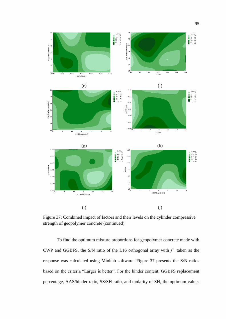
95
(e) (f)
(g) (h)
(i) (j)
Figure 37: Combined impact of factors and their levels on the cylinder compressive
strength of geopolymer concrete (continued)
To find the optimum mixture proportions for geopolymer concrete made with
CWP and GGBFS, the S/N ratio of the L16 orthogonal array with f’c taken as the
response was calculated using Minitab software. Figure 37 presents the S/N ratios
based on the criteria “ arger is better” For the binder content, GGBFS replacement
percentage, AAS/binder ratio, SS/SH ratio, and molarity of SH, the optimum values

96
were 450 kg/m3, 60%, 0.50, 1.5, and 10 M, respectively. The S/N ratios are shown in
Table 18. The optimum mix is denoted by A2B3C1D2E2. Furthermore, it is worth
noting that the lowest S N ratios for factor ‘A’, binder content, were those of and
550 kg/m3. This shows that CWP-GGBFS blended geopolymer concrete does not
necessarily produce higher strength if more binder is used in the mix.
Figure 38: Signal-to-noise ratios of Taguchi design for cylinder compressive strength
Table 18: Response Table for Signal-to-Noise Ratios
Level A B C D E
1 29.499 26.020 31.068 4.205 26.063
2 30.672 15.627 17.040 30.169 29.539
3 14.911 30.145 16.322 28.336 15.635
4 15.083 18.374 25.735 27.455 18.929
Delta 15.760 14.518 14.746 25.964 13.904
Rank 2 4 3 1 5

97
5.2 Taguchi Optimization by Best Worst Method
Taguchi optimization by Best Worst Method considering nine, five and two
quality criteria are explained in the below subsections.
5.2.1 Nine Quality Criteria
The Best-Worst method (BWM) is an optimization technique that is applied
to the Taguchi method. It shows the preference of the most significant, i.e. best, and
least significant, i.e. worst, criteria against all other criteria. The steps explained in
Chapter 3 are adopted to obtain the optimum mixes while considering different
quality criteria as follows:
Step 1: Nine quality criteria were considered for the decision-making process,
including compressive strength, water absorption, sorptivity, abrasion resistance,
modulus of rupture, split tensile strength, modulus of elasticity, bulk resistivity, and
ultrasonic pulse velocity. For each quality criterion, the target value, best experiment
(mix), and worst experiment are determined as shown in Table 19. It is worth noting
that the target value of all quality criteria is ‘ arger is better’ except water absorption
and sorptivity since lower values of these two criteria would indicate enhanced
durability performance.
Step 2: Compressive strength and ultrasonic pulse velocity were chosen as the
best and worst criteria, respectively. Tables 20 and 21 display the comparison of best
and worst quality criteria to others, respectively. The weight of each quality criteria
and the consistency ratio ξL were calculated using Equations (12) and (13). Results
are given in Table 22. For the pair wise comparison, it is required that the
consistency ratio be less than 0.1. In this work, it is 0.06.

98
Table 19: Selected nine quality criteria, target value, and best and worst
No. Symbol Quality
criteria
Unit Target
Value
Best
Experiment
Worst
Experiment
1 Q1 Compressive
strength
MPa Larger is
better
T11 T10
2 Q2 Water
absorption
% Smaller is
better
T11 T10
3 Q3 Sorptivity mm √s Smaller is
better
T11 T15
4 Q4 Abrasion
Resistance
% Smaller is
better
T11 T10
5 Q5 Modulus of
Rupture
MPa Larger is
better
T11 T10
6 Q6 Splitting tensile
strength
MPa Larger is
better
T11 T10
7 Q7 Modulus of
Elasticity
GPa Larger is
better
T11 T10
8 Q8 Bulk Resistivity kΩ cm Larger is
better
T11 T13
9 Q9 Ultrasonic pulse
velocity
m/s Larger is
better
T11 T10
Table 20: Comparision of best quality criteria to other eight quality criteria
Quality Criteria Q1 Q2 Q3 Q4 Q5 Q6 Q7 Q8 Q9
Best Criteria Q1 1 2 3 5 4 6 8 6 9
Table 21: Comparision of worst quality criteria to other eight quality criteria
Quality Criteria Q1 Q2 Q3 Q4 Q5 Q6 Q7 Q8 Q9
Worst Criteria Q9 9 8 7 5 6 4 2 3 1
Table 22: Weights of the nine quality criteria
No. Symbol Quality Criteria Criteria
weight 1 Q1 Compressive strength 28 days (MPa) 0.31179394
2 Q2 Water absorption (%) 0.18978762
3 Q3 Sorptivity (mm √s) 0.12652508
4 Q4 Abrasion Resistance (Mass loss in %) 0.07591505
5 Q5 Modulus of Rupture (MPa) 0.09489381
6 Q6 Splitting tensile strength 28 days (MPa) 0.06326254
7 Q7 Modulus of Elasticity (MPa) 0.0474469
8 Q8 Bulk Resistivity (Ω cm) 0.06326254
9 Q9 Ultrasonic pulse velocity (m/s) 0.02711252
Consistency ratio, Ksi 0.06778129

99
Step 3: The results of the Taguchi Orthogonal experiments (mixes) are
presented in Table 23. The reference comparison of best experiments with respect to
each quality criteria was ranked using a scale of 1 to 9. The best experiments can
easily be identified by scrutinizing the experiment results. For instance, the best and
worst experiments for compressive strength (Q1) were T11 and T10, respectively.
The same procedure was applied to other quality criteria. The respective comparison
to the best and worst experiments are shown in Tables 24 and 25.
Step 4: The weight of each experiment for each quality criteria was determined
with respect to all quality criteria in a similar way to Step 2. Results of the relative
weights are shown in Table 26. The relative weights were then multiplied by the
weights of Table 22 to obtain the total weight for each experiment, as shown in Table
27. Thus, the multi-objective problem was converted into a single objective problem
[47]. Also, it is worth noting that the consistency ratio of the estimated weight was
less than 0.1; thus, the estimated weights were considered reliable.
Step 5: The S/N ratio was calculated using Minitab for the total weight of each
experiment, considering the target ‘ arger is better’, as per quation 9 alues are
shown in Table 27 and plotted in Figure 38. Based on the obtained results, mixture
A2B3C1D2E2 was found to be the optimum mix with a binder content of 450 kg/m3,
GGBFS replacement percentage of 60%, AAS/binder ratio of 0.50, SS/SH ratio of
1.5, and SH molarity of 10 M.
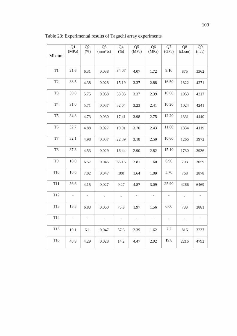
100
Table 23: Experimental results of Taguchi array experiments
Mixture
Q1
(MPa) Q2
(%) Q3
(mm √s) Q4
(%) Q5
(MPa) Q6
(MPa) Q7
(GPa) Q8
(Ω cm) Q9
(m/s)
T1 21.6 6.31 0.038 34.07 4.07 1.72 9.10 875 3362
T2 38.5 4.38 0.028 15.19 3.37 2.88 16.50 1822 4271
T3 30.8 5.75 0.038 33.85 3.37 2.39 10.60 1053 4217
T4 31.0 5.71 0.037 32.04 3.23 2.41 10.20 1024 4241
T5 34.8 4.73 0.030 17.41 3.98 2.75 12.20 1331 4440
T6 32.7 4.88 0.027 19.91 3.70 2.43 11.80 1334 4119
T7 32.1 4.98 0.037 22.39 3.18 2.59 10.60 1266 3972
T8 37.3 4.53 0.029 16.44 2.90 2.82 15.10 1730 3936
T9 16.0 6.57 0.045 66.16 2.81 1.60 6.90 793 3059
T10 10.6 7.02 0.047 100 1.64 1.09 3.70 768 2878
T11 56.6 4.15 0.027 9.27 4.87 3.09 25.90 4266 6469
T12 - - - - - - - - -
T13 13.3 6.83 0.050 75.8 1.97 1.56 6.00 733 2881
T14 - - - - - - - - -
T15 19.1 6.1 0.047 57.3 2.39 1.62 7.2 816 3237
T16 40.9 4.29 0.028 14.2 4.47 2.92 19.8 2216 4792
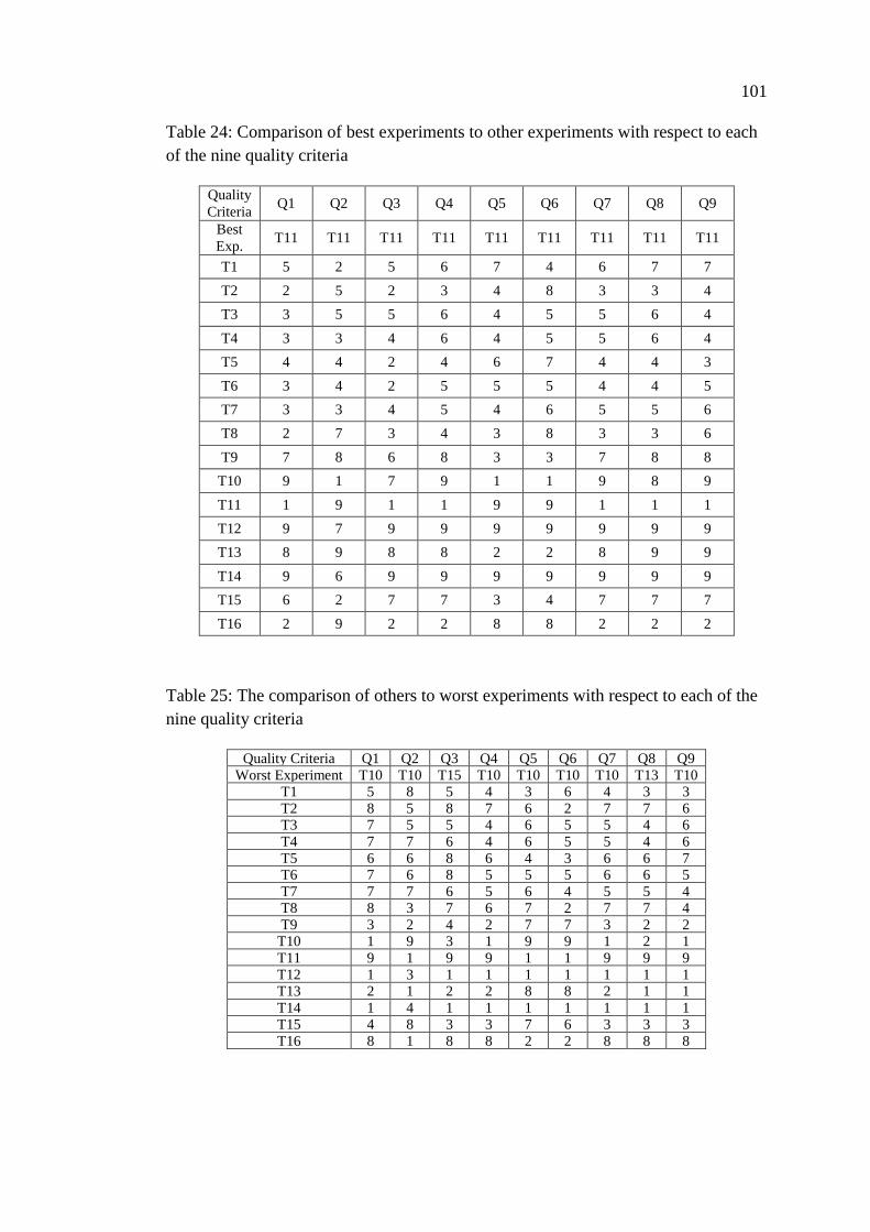
101
Table 24: Comparison of best experiments to other experiments with respect to each
of the nine quality criteria
Quality
Criteria Q1 Q2 Q3 Q4 Q5 Q6 Q7 Q8 Q9
Best
Exp. T11 T11 T11 T11 T11 T11 T11 T11 T11
T1 5 2 5 6 7 4 6 7 7
T2 2 5 2 3 4 8 3 3 4
T3 3 5 5 6 4 5 5 6 4
T4 3 3 4 6 4 5 5 6 4
T5 4 4 2 4 6 7 4 4 3
T6 3 4 2 5 5 5 4 4 5
T7 3 3 4 5 4 6 5 5 6
T8 2 7 3 4 3 8 3 3 6
T9 7 8 6 8 3 3 7 8 8
T10 9 1 7 9 1 1 9 8 9
T11 1 9 1 1 9 9 1 1 1
T12 9 7 9 9 9 9 9 9 9
T13 8 9 8 8 2 2 8 9 9
T14 9 6 9 9 9 9 9 9 9
T15 6 2 7 7 3 4 7 7 7
T16 2 9 2 2 8 8 2 2 2
Table 25: The comparison of others to worst experiments with respect to each of the
nine quality criteria
Quality Criteria Q1 Q2 Q3 Q4 Q5 Q6 Q7 Q8 Q9
Worst Experiment T10 T10 T15 T10 T10 T10 T10 T13 T10 T1 5 8 5 4 3 6 4 3 3
T2 8 5 8 7 6 2 7 7 6 T3 7 5 5 4 6 5 5 4 6
T4 7 7 6 4 6 5 5 4 6
T5 6 6 8 6 4 3 6 6 7 T6 7 6 8 5 5 5 6 6 5
T7 7 7 6 5 6 4 5 5 4 T8 8 3 7 6 7 2 7 7 4
T9 3 2 4 2 7 7 3 2 2 T10 1 9 3 1 9 9 1 2 1
T11 9 1 9 9 1 1 9 9 9
T12 1 3 1 1 1 1 1 1 1 T13 2 1 2 2 8 8 2 1 1
T14 1 4 1 1 1 1 1 1 1 T15 4 8 3 3 7 6 3 3 3
T16 8 1 8 8 2 2 8 8 8

102
Table 26: The relative weight of each experiment with respect to each of the nine
quality characteristics
Experiments Quality Characteristics
Q1 Q2 Q3 Q4 Q5 Q6 Q7 Q8 Q9
T1 0.04
1
0.117 0.04
0
0.04
4
0.03
3
0.06
6
0.04
2
0.03
7
0.03
8 T2 0.10
3
0.046 0.10
3
0.08
1
0.05
8
0.03
3
0.08
4
0.08
6
0.06
6 T3 0.06
8
0.046 0.04
1
0.04
4
0.05
8
0.05
3
0.05
0
0.04
3
0.06
6 T4 0.06
8
0.078 0.05
1
0.04
4
0.05
8
0.05
3
0.05
0
0.04
3
0.06
6 T5 0.05
1
0.058 0.10
3
0.06
6
0.03
9
0.03
8
0.06
3
0.06
4
0.08
8 T6 0.06
8
0.058 0.10
3
0.05
3
0.04
7
0.05
3
0.06
3
0.06
4
0.05
3 T7 0.06
8
0.078 0.05
1
0.05
3
0.05
8
0.04
4
0.05
0
0.05
1
0.04
4 T8 0.10
3
0.033 0.06
9
0.06
6
0.07
8
0.03
3
0.08
4
0.08
6
0.04
4 T9 0.02
9
0.029 0.03
4
0.03
3
0.07
8
0.08
9
0.03
6
0.03
2
0.03
3 T10 0.01
4
0.192 0.02
9
0.01
9
0.19
3
0.22
0
0.01
8
0.03
2
0.01
9 T11 0.16
9
0.016 0.17
0
0.21
9
0.01
6
0.01
9
0.20
7
0.21
3
0.21
8 T12 0.02
2
0.033 0.01
4
0.02
9
0.02
6
0.02
9
0.02
8
0.01
8
0.02
9 T13 0.02
5
0.026 0.02
5
0.03
3
0.11
7
0.13
3
0.03
1
0.02
8
0.02
9 T14 0.02
2
0.039 0.02
3
0.02
9
0.02
6
0.02
9
0.02
8
0.02
8
0.02
9 T15 0.03
4
0.117 0.02
9
0.03
8
0.07
8
0.06
6
0.03
6
0.03
7
0.03
8 T16 0.10
3
0.026 0.10
3
0.13
3
0.02
9
0.03
3
0.12
6
0.12
9
0.13
3 Sum 1.00
0
1.000 1.00
0
1.00
0
1.00
0
1.00
0
1.00
0
1.00
0
1.00
0
Consistency
ratio
0.03 0.04 0.03 0.04 0.04 0.04 0.04 0.04 0.04
Figure 39: S/N Ratio plot of nine quality criteria (Q1 to Q9) using BWM-based
Taguchi method

103
Table 27: Total weight and S/N ratios for each experiment (nine quality criteria)
Experiments Total
Weight
S/N ratios for
Total weight T1 0.05662 -27.8061
T2 0.08005 -20.5914
T3 0.05497 -25.1979
T4 0.06222 -24.9927
T5 0.06113 -23.7621
T6 0.06625 -23.5768
T7 0.06228 -24.6470
T8 0.07269 -21.8111
T9 0.03946 -27.9027
T10 0.08210 -26.2524
T11 0.12651 -15.9215
T12 0.02534 -32.4238
T13 0.04260 -27.2863
T14 0.02809 -31.8293
T15 0.05646 -27.6175
T16 0.08322 -19.9524
5.2.2 Five Quality Criteria
While the BWM optimized Taguchi technique is a reliable means to optimize
experimental design, the use of nine quality criteria can require extensive testing.
Therefore, an attempt is made to utilize five quality criteria, including Q1, Q2, Q5,
Q6, and Q8, as shown in Table 28. These criteria represent part of the mechanical
and durability properties of CWP-GGBFS blended geopolymer concrete. Other
quality characteristics Q3, Q4, Q7, and Q9 were not considered because they are
related to the other quality characteristics. The same steps as those listed in section
5.2.1 were used. The comparison of the best and worst quality criteria to the
remaining ones is shown in Table 29 and 30, respectively. Furthermore, the weights
of each of the five quality criteria were calculated and presented in Table 31. Then, a
comparison among the experiments with respect to the best and worst ones is carried
out. Results are tabulated in Tables 32 and 33. These results are used to obtain the

104
relative weights shown in Table 34 and the total weights of Table 35. By inputting
the total weights in Minitab, the S/N ratios are obtained as in Table 35 and Figure 39.
The findings revealed that the optimum mix is denoted as A2B3C1D2E2.
Table 28: Selected five quality criteria, target value, and best and worst experiment
No. Symbol Quality
criteria
Unit Target
Value
Best
Experiment
Worst
Experiment
1 Q1 Compressive
strength
MPa Larger is
better
T11 T10
2 Q2 Water
absorption
% Smaller is
better
T11 T10
5 Q5 Modulus of
Rupture
MPa Larger is
better
T11 T10
6 Q6 Splitting tensile
strength
MPa Larger is
better
T11 T10
8 Q8 Bulk Resistivity kΩ cm Larger is
better
T11 T13
Table 29: Comparison of best quality criteria to other four quality criteria
Quality Criteria Q1 Q2 Q5 Q6 Q8
Best Criteria Q1 1 2 4 6 9
Table 30: Comparison of worst quality criteria to other four quality criteria
Quality Criteria Q1 Q2 Q5 Q6 Q8
Worst Criteria
Q8
9 8 6 4 1
Table 29: Weights of the five quality criteria
No. Symbol Quality Criteria Criteria
weight 1 Q1 Compressive strength 28 days (MPa) 0.453947
2 Q2 Water absorption (%) 0.276316
5 Q5 Modulus of Rupture (MPa) 0.138158
6 Q6 Splitting tensile strength 28 days (MPa) 0.092105
8 Q8 Bulk Resistivity (Ω cm) 0.039474
Consistency ratio, Ksi 0.098684

105
Table 30: Comparison of best experiments to other experiments with respect to each
of the five quality criteria
Quality
Criteria Q1 Q2 Q5 Q6 Q8
Best
Exp. T11 T11 T11 T11 T11
T1 5 7 7 4 7
T2 2 2 4 8 3
T3 3 5 4 5 6
T4 3 5 4 5 6
T5 4 3 6 7 4
T6 3 4 5 5 4
T7 3 4 4 6 5
T8 2 3 3 8 3
T9 7 7 3 3 8
T10 9 9 1 1 8
T11 1 1 9 9 1
T12 9 9 9 9 9
T13 8 8 2 2 9
T14 9 9 9 9 9
T15 6 6 3 4 7
T16 2 2 8 8 2
Table 31: The comparison of others to worst experiments with respect to each of the
five quality criteria
Quality Criteria Q1 Q2 Q5 Q6 Q8
Worst Experiment T10 T10 T10 T10 T13
T1 5 3 3 6 3
T2 8 8 6 2 7
T3 7 5 6 5 4
T4 7 5 6 5 4
T5 6 7 4 3 6
T6 7 6 5 5 6
T7 7 6 6 4 5
T8 8 7 7 2 7
T9 3 3 7 7 2
T10 1 1 9 9 2
T11 9 9 1 1 9
T12 1 1 1 1 1
T13 2 2 8 8 1
T14 1 1 1 1 1
T15 4 4 7 6 3
T16 8 8 2 2 8

106
Table 32: The relative weight of each experiment with respect to each of the five
quality characteristics
Experiments Quality Characteristics
Q1 Q2 Q5 Q6 Q8
T1 0.041383 0.033541 0.033617 0.066971 0.037098
T2 0.103457 0.117395 0.058829 0.033486 0.086562
T3 0.068971 0.046958 0.058829 0.053577 0.043281
T4 0.068971 0.046958 0.058829 0.053577 0.043281
T5 0.051728 0.078263 0.039219 0.038269 0.064922
T6 0.068971 0.058697 0.047063 0.053577 0.064922
T7 0.068971 0.058697 0.058829 0.044648 0.051937
T8 0.103457 0.078263 0.078439 0.033486 0.086562
T9 0.029559 0.033541 0.078439 0.089295 0.032461
T10 0.014780 0.016771 0.193295 0.220049 0.032461
T11 0.169965 0.192863 0.016808 0.019135 0.213314
T12 0.022990 0.026088 0.026146 0.029765 0.018549
T13 0.025864 0.029349 0.117658 0.133943 0.028854
T14 0.022990 0.026088 0.026146 0.029765 0.028854
T15 0.034486 0.039132 0.078439 0.066971 0.037098
T16 0.103457 0.117395 0.029415 0.033486 0.129843
Sum 1.00000 1.00000 1.00000 1.00000 1.00000
Consistency
ratio
0.03695 0.04193 0.04202 0.04784 0.04637
Table 33: Total weight and S/N ratios for each experiment (five quality criteria)
Experiments Total
Weight
S/N ratios for
Total weight
T1 0.04033 -23.9444 T2 0.09403 -22.5490 T3 0.05906 -24.5748 T4 0.05906 -23.3875 T5 0.05661 -25.8134 T6 0.06153 -24.2186 T7 0.06182 -23.4494 T8 0.08593 -22.6660 T9 0.04303 -27.5618 T10 0.05960 -19.3111 T11 0.14295 -20.5103 T12 0.02473 -31.4404 T13 0.04958 -26.2529 T14 0.02514 -30.8297 T15 0.04494 -23.5354 T16 0.09168 -23.5506

107
Figure 40: S/N Ratio plot of Five quality criteria (Q1, Q2, Q5, Q6, and Q8) using
BWM-based Taguchi method
5.2.3 Two Quality Criteria
The BWM optimization technique typically incorporates quality criteria for
multiple experiments without being directly related. This ensures that each criterion
is considered in the optimization process. However, since some of these criteria or
properties were found to be related in Chapter 4, a modification to the before-
mentioned BWM has been proposed by taking only two quality criteria, the
compressive strength and water absorption, representing the mechanical and
durability performance of CWP-GGBFS blended geopolymer concrete. The results
associated with this technique are shown in Tables 36-43. Based on the total weights,
the S/N ratios are plotted in Figure 40. The optimum mix is labeled A2B3C1D2E2.

108
Table 34: Selected five quality criteria, target value, and best and worst experiment
No. Symbol Quality criteria Target
Value
Best
Experiment
Worst
Experiment
1 Q1 Compressive strength
28 days (MPa)
Larger the
better
T11 T10
2 Q2 Water absorption (%) Smaller the
better
T11 T10
Table 35: Comparison of best quality criteria to the other quality criteria
Quality Criteria Q1 Q2
Best Criteria Q1 1 2
Table 36: Comparison of worst quality criteria to the other quality criteria
Quality Criteria Worst criteria Q2
Q1 9
Q2 8
Table 37: Weights of the two quality criteria
No. Symbol Quality
Criteria
Criteria
weight
1 Q1 Compressive strength 28 days (MPa) 0.5
2 Q2 Water absorption (%) 0.5
Consistency ratio, Ksi 0.5
Three BWM-based Taguchi methods were adopted. While one employed
nine quality criteria, the other two utilized five and two criteria only. The
contribution of each factor based on the three methods is calculated using Minitab
and presented in Table 44. Findings revealed that the highest contributor was the
SS/SH ratio followed by the AAS/binder ratio, the molarity of the SH solution, and
GGBFS replacement percentage. Of the five factors, the binder content had the least
contribution, and therefore, was the least impactful on the optimization.
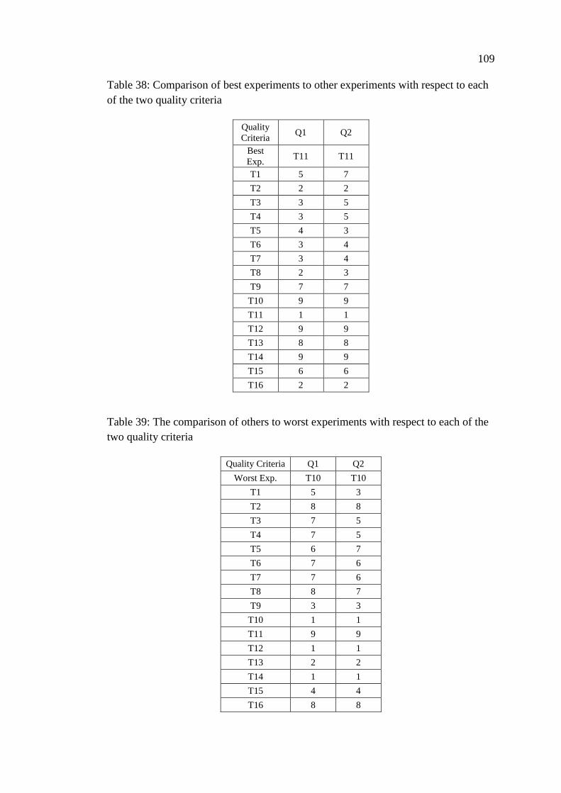
109
Table 38: Comparison of best experiments to other experiments with respect to each
of the two quality criteria
Quality
Criteria Q1 Q2
Best
Exp. T11 T11
T1 5 7
T2 2 2
T3 3 5
T4 3 5
T5 4 3
T6 3 4
T7 3 4
T8 2 3
T9 7 7
T10 9 9
T11 1 1
T12 9 9
T13 8 8
T14 9 9
T15 6 6
T16 2 2
Table 39: The comparison of others to worst experiments with respect to each of the
two quality criteria
Quality Criteria Q1 Q2
Worst Exp. T10 T10
T1 5 3
T2 8 8
T3 7 5
T4 7 5
T5 6 7
T6 7 6
T7 7 6
T8 8 7
T9 3 3
T10 1 1
T11 9 9
T12 1 1
T13 2 2
T14 1 1
T15 4 4
T16 8 8

110
Table 40: The relative weight of each experiment with respect to each of the two
quality characteristics
Experiments Quality Characteristics
Q1 Q2
T1 0.04138 0.03354
T2 0.10346 0.11739
T3 0.06897 0.04696
T4 0.06897 0.04696
T5 0.05173 0.07826
T6 0.06897 0.05870
T7 0.06897 0.05870
T8 0.10346 0.07826
T9 0.02956 0.03354
T10 0.01478 0.01677
T11 0.16996 0.19286
T12 0.02299 0.02609
T13 0.02586 0.02935
T14 0.02299 0.02609
T15 0.03449 0.03913
T16 0.10346 0.11739
Sum 1.00000 1.00000
Consistency ratio 0.03695 0.04193

111
Table 41: Total weight and its S/N ratios for each experiment (two quality criteria)
Experiments Total
Weight
S/N ratios for
Total weight
T1 0.03746 -28.5282
T2 0.11043 -19.1386
T3 0.05796 -24.7367
T4 0.05796 -24.7367
T5 0.06500 -23.7423
T6 0.06383 -23.8989
T7 0.06383 -23.8989
T8 0.09086 -20.8325
T9 0.03155 -30.0199
T10 0.01578 -36.0405
T11 0.18141 -14.8266
T12 0.02454 -32.2028
T13 0.02761 -31.1798
T14 0.02454 -32.2028
T15 0.03681 -28.6810
T16 0.11043 -19.1386
Figure 41: SN Ratio plot of Two quality criteria (Q1 and Q2) using BWM-based
Taguchi method

112
Table 42: Contribution of factors in the three BWM-based Taguchi methods
Factor
Contribution
Q1-Q9 (%)
Contribution
Q1,Q2,Q5,Q6,Q8 (%)
Contribution
Q1,Q2 (%)
Binder
content
3.63 4.13 3.46
GGBFS
Replacement
12.14 13.99 16.28
AAS/Binder 27.12 19.30 26.58
SS/SH 42.17 50.77 34.86
Molarity
of SH
14.94 11.81 18.83
Total 100.00 100.00 100.00
5.3 Taguchi Optimization by TOPSIS Method
Taguchi optimization by TOPSIS Method considering nine, five and two
quality criteria are explained in the below subsections.
5.3.1 Nine Quality Criteria
Another attempt was made to optimize the mixture proportions by modifying
the Taguchi method using TOPSIS. The steps to obtain the optimum mix are as
follows:

113
Table 43: S/N ratios decision matrix for nine quality criteria
Experiment/
Quality criteria Q1 Q2 Q3 Q4 Q5 Q6 Q7 Q8 Q9
T1 26.6
9
16.00 28.40 30.65 12.20 4.71 19.18 58.84 70.53
T2 31.7
1
12.83 31.06 23.63 10.56 9.19 24.35 65.21 72.61
T3 29.7
7
15.19 28.40 30.59 10.56 7.57 20.51 60.45 72.50
T4 29.8
3
15.13 28.64 30.11 10.19 7.64 20.17 60.20 72.55
T5 30.8
3
13.50 31.37 24.82 12.00 8.79 21.73 62.48 72.95
T6 30.2
9
13.77 31.37 25.98 11.36 7.71 21.44 62.50 72.30
T7 30.1
3
13.94 28.64 27.00 10.06 8.27 20.51 62.05 71.98
T8 31.4
3
13.12 30.75 24.32 9.26 9.00 23.58 64.76 71.90
T9 24.0
8
16.35 26.94 36.41 8.97 4.08 16.78 57.98 69.71
T10 20.5
1
16.93 26.56 40.00 4.29 0.75 11.36 57.71 69.18
T11 35.0
6
12.36 31.37 19.34 13.75 9.80 28.27 72.60 76.22
T12 60.0
0
100.0
0
100.0
0
100.0
0
-
60.00
-
60.00
-
60.00
-
60.00
-
60.00 T13 22.4
8
16.69 26.02 37.59 5.88 3.86 15.56 57.30 69.19
T14 60.0
0
100.0
0
100.0
0
100.0
0
-
60.00
-
60.00
-
60.00
-
60.00
-
60.00 T15 25.6
2
15.71 26.56 35.16 7.57 4.19 17.15 58.23 70.20
T16 32.2
3
12.65 31.06 23.05 13.01 9.31 25.93 66.91 73.61
Square Root
of Sum
of Squares
137.
4 151.6 178.5 180.0 93.1 89.1 115.3 247.3 281.8
Step 1: The decision matrix was formed using the characteristic values of
alternatives (experiments) and attributes (calculated S/N ratios of responses). Thus,
the S/N ratios decision matrix was formed as shown in Table 45. Each value is
obtained by inputting the L16 orthogonal array and experimental values of each
criterion in Minitab and obtaining the S/N ratio. The last row represents the square
root of the sum of squares of each column.
Step 2: The normalized decision matrix is determined using the vector
normalization equation of Equation (15). The normalized matrix for the nine quality

114
criteria is shown in Table 46. It is worth noting that the top row is the weight of each
quality, which can be found in Table 22. The other data points are obtained by
dividing the corresponding value in Table 45 by the bottom row of Table 45.
Table 44: Normalized decision matrix for nine quality criteria
Step 3: The weighted normalized decision matrix was calculated using
Equation (16) and is shown in columns 2 to 10 of Table 47. Each data point
represents the product of that corresponding point in Table 46 and the weight (first
row of Table 46). The positive ideal solution (A+) and negative ideal solution (A
-)
were computed using Equations (17) and (18), respectively. They represent the
respective maximum and minimum values in each column. The estimated (A+) and
Experiment/
Weight 0.312 0.190 0.127 0.076 0.095 0.063 0.047 0.063 0.027
T1 0.194 0.116 0.159 0.170 0.131 0.053 0.166 0.238 0.250
T2 0.231 0.093 0.174 0.131 0.113 0.103 0.211 0.264 0.258
T3 0.217 0.111 0.159 0.170 0.113 0.085 0.178 0.244 0.257
T4 0.217 0.110 0.160 0.167 0.109 0.086 0.175 0.243 0.257
T5 0.224 0.098 0.176 0.138 0.129 0.099 0.188 0.253 0.259
T6 0.220 0.100 0.176 0.144 0.122 0.087 0.186 0.253 0.256
T7 0.219 0.101 0.160 0.150 0.108 0.093 0.178 0.251 0.255
T8 0.229 0.095 0.172 0.135 0.099 0.101 0.204 0.262 0.255
T9 0.175 0.119 0.151 0.202 0.096 0.046 0.145 0.234 0.247
T10 0.149 0.123 0.149 0.222 0.046 0.008 0.098 0.233 0.245
T11 0.255 0.090 0.176 0.107 0.148 0.110 0.245 0.294 0.270
T12 -0.437 0.728 0.560 0.555 -0.644 -0.673 -0.520 -0.243 -0.213
T13 0.164 0.121 0.146 0.209 0.063 0.043 0.135 0.232 0.245
T14 -0.437 0.728 0.560 0.555 -0.644 -0.673 -0.520 -0.243 -0.213
T15 0.186 0.114 0.149 0.195 0.081 0.047 0.149 0.235 0.249
T16 0.235 0.092 0.174 0.128 0.140 0.104 0.225 0.271 0.261

115
(A-) values are shown in the last two rows of Table 47. Furthermore, the separation
measures of the alternatives to the positive ideal solution (Si+) and the distance from
the negative ideal solution (Si-) were estimated using Equations (19) and (20),
respectively. The estimated values are given in columns 11 and 12 of Table 47.
Lastly, the ranking or performance score was determined using Equation (21) and
presented in the last column of Table 47.
Table 45: Weighted normalized decision matrix for nine quality criteria
Step 4: The performance score is inputted alongside an L16 orthogonal array in
Minitab to calculate the S/N ratios shown in Figure 41. The target value considered
was ‘ arger is better’ Based on the plot, the optimum mix can be denoted as
A2B3C1D2E2.
vi1 vi2 vi3 vi4 vi5 vi6 vi7 vi8 vi9 Si+ Si- Score
T1 0.06 0.02 0.02 0.01 0.01 0.01 0.01 0.02 0.01 0.13 0.22 0.63 T2 0.07 0.01 0.02 0.01 0.01 0.01 0.01 0.02 0.01 0.13 0.23 0.63
T3 0.06 0.02 0.02 0.01 0.01 0.01 0.01 0.02 0.01 0.13 0.23 0.63
T4 0.06 0.02 0.02 0.01 0.01 0.01 0.01 0.02 0.01 0.13 0.23 0.63 T5 0.07 0.02 0.02 0.01 0.01 0.01 0.01 0.02 0.01 0.13 0.23 0.63
T6 0.06 0.02 0.02 0.01 0.01 0.01 0.01 0.02 0.01 0.13 0.23 0.63 T7 0.07 0.02 0.02 0.01 0.01 0.01 0.01 0.02 0.01 0.13 0.23 0.63
T8 0.07 0.02 0.02 0.01 0.01 0.01 0.01 0.02 0.01 0.13 0.23 0.63 T9 0.05 0.02 0.02 0.02 0.01 0.01 0.01 0.02 0.01 0.13 0.21 0.62
T1
0
0.04 0.02 0.02 0.02 0.01 0.01 0.01 0.02 0.01 0.13 0.20 0.60
T1
1
0.08 0.02 0.02 0.01 0.01 0.01 0.01 0.02 0.01 0.14 0.24 0.64 T1
2
-0.13 0.14 0.07 0.04 -0.06 -0.04 -0.03 -0.02 -0.01 0.24 0.02 0.36
T1
3
0.05 0.02 0.02 0.02 0.01 0.01 0.01 0.02 0.01 0.13 0.21 0.61 T1
4
-0.13 0.14 0.07 0.04 -0.06 -0.04 -0.03 -0.02 -0.01 0.24 0.02 0.36
T1
5
0.05 0.02 0.02 0.02 0.01 0.01 0.01 0.02 0.01 0.13 0.22 0.62
T1
6
0.07 0.02 0.02 0.01 0.01 0.01 0.01 0.02 0.01 0.13 0.23 0.63 A+ 0.08 0.14 0.07 0.04 0.01 0.01 0.01 0.02 0.01
A- -0.13 0.02 0.02 0.01 -0.06 -0.04 -0.03 -0.02 -0.01

116
Figure 42: Optimal level for each factor by TOPSIS optimised Taguchi method
considering all quality criteria (Q1 to Q9)
5.3.2 Five and Two Quality Criteria
Similar to the reasoning given for the BWM method, an attempt has been
made to reduce the number of quality criteria to five and two. The results associated
with the five quality criteria TOPSIS-based optimization technique are shown in
Tables 48 and 49. The obtained S/N of Figure 42 shows an optimum mix with a
binder content of 450 kg/m3, GGBFS replacement percentage of 60%, AAS/binder
ratio of 0.50, SS/SH ratio of 1.5, and SH molarity of 10 M. Similarly, the results of
the two quality criteria TOPSIS method (Tables 50 and 51 and Figure 43) presented
the same optimum mix.
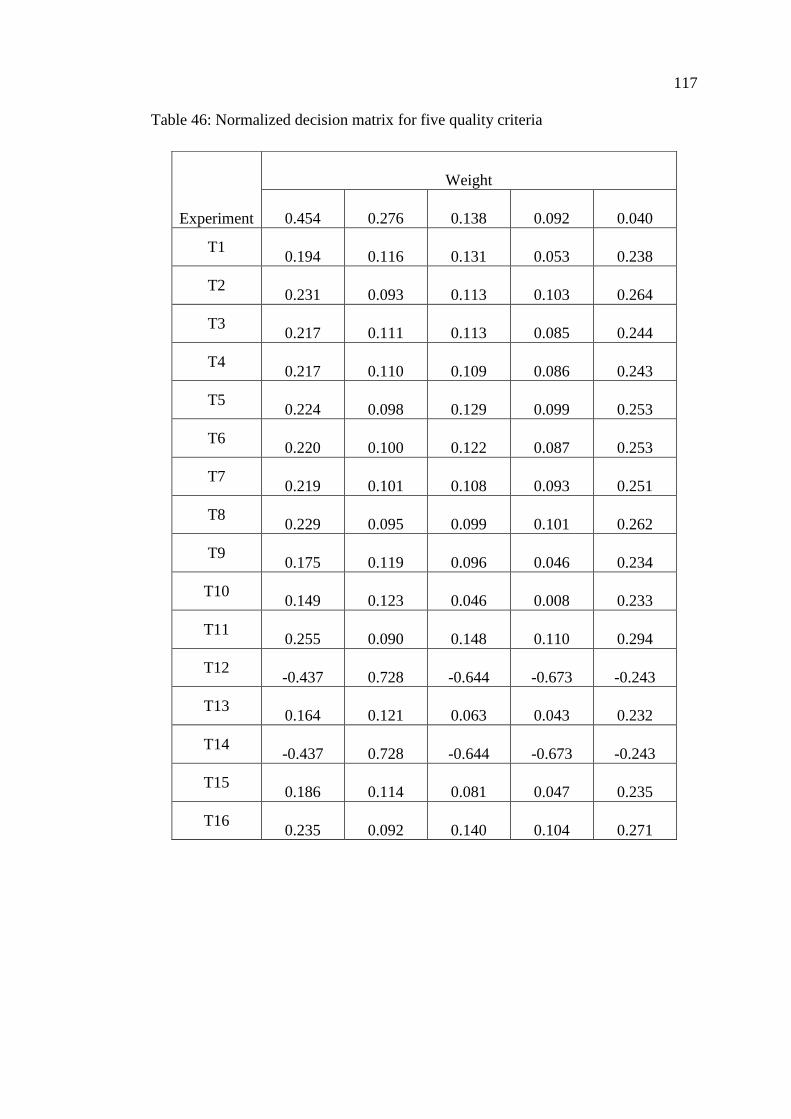
117
Table 46: Normalized decision matrix for five quality criteria
Experiment
Weight
0.454 0.276 0.138 0.092 0.040
T1 0.194 0.116 0.131 0.053 0.238
T2 0.231 0.093 0.113 0.103 0.264
T3 0.217 0.111 0.113 0.085 0.244
T4 0.217 0.110 0.109 0.086 0.243
T5 0.224 0.098 0.129 0.099 0.253
T6 0.220 0.100 0.122 0.087 0.253
T7 0.219 0.101 0.108 0.093 0.251
T8 0.229 0.095 0.099 0.101 0.262
T9 0.175 0.119 0.096 0.046 0.234
T10 0.149 0.123 0.046 0.008 0.233
T11 0.255 0.090 0.148 0.110 0.294
T12 -0.437 0.728 -0.644 -0.673 -0.243
T13 0.164 0.121 0.063 0.043 0.232
T14 -0.437 0.728 -0.644 -0.673 -0.243
T15 0.186 0.114 0.081 0.047 0.235
T16 0.235 0.092 0.140 0.104 0.271

118
Table 47: Weighted normalized decision matrix for five quality criteria
vi1 vi2 vi5 vi6 vi8 Si+ Si- Score
T1 0.088 0.032 0.018 0.005 0.009 0.171 0.314 0.647
T2 0.105 0.026 0.016 0.009 0.010 0.176 0.329 0.652
T3 0.098 0.031 0.016 0.008 0.010 0.171 0.323 0.653
T4 0.099 0.030 0.015 0.008 0.010 0.172 0.323 0.653
T5 0.102 0.027 0.018 0.009 0.010 0.175 0.327 0.652
T6 0.100 0.028 0.017 0.008 0.010 0.174 0.325 0.651
T7 0.100 0.028 0.015 0.009 0.010 0.174 0.324 0.651
T8 0.104 0.026 0.014 0.009 0.010 0.175 0.327 0.651
T9 0.080 0.033 0.013 0.004 0.009 0.172 0.304 0.638
T10 0.068 0.034 0.006 0.001 0.009 0.175 0.290 0.624
T11 0.116 0.025 0.020 0.010 0.012 0.176 0.341 0.659
T12 -0.198 0.201 -0.089 -0.062 -0.010 0.341 0.176 0.341
T13 0.074 0.034 0.009 0.004 0.009 0.173 0.298 0.632
T14 -0.198 0.201 -0.089 -0.062 -0.010 0.341 0.176 0.341
T15 0.085 0.032 0.011 0.004 0.009 0.173 0.308 0.641
T16 0.106 0.025 0.019 0.010 0.011 0.176 0.332 0.654
A+ 0.116 0.201 0.020 0.010 0.012
A- -0.198 0.025 -0.089 -0.062 -0.010

119
Figure 43: Optimal level for each factor by TOPSIS optimised Taguchi method
considering Q1, Q2, Q5, Q6, and Q8 quality criteria
Table 48: Normalized decision matrix for two quality criteria
Experiment
Weight
0.5 0.5
T1 0.194 0.116
T2 0.231 0.093
T3 0.217 0.111
T4 0.217 0.110
T5 0.224 0.098
T6 0.220 0.100
T7 0.219 0.101
T8 0.229 0.095
T9 0.175 0.119
T10 0.149 0.123
T11 0.255 0.090
T12 -0.437 0.728
T13 0.164 0.121
T14 -0.437 0.728
T15 0.186 0.114
T16 0.235 0.092

120
Table 49: Weighted normalized decision matrix for two quality criteria
vi1 vi2 Si+ Si- Score
T1 0.097 0.058 0.307 0.316 0.507
T2 0.115 0.047 0.317 0.334 0.513
T3 0.108 0.055 0.309 0.327 0.514
T4 0.109 0.055 0.309 0.327 0.514
T5 0.112 0.049 0.315 0.330 0.512
T6 0.110 0.050 0.314 0.329 0.511
T7 0.110 0.051 0.314 0.328 0.511
T8 0.114 0.048 0.316 0.333 0.513
T9 0.088 0.059 0.307 0.306 0.499
T10 0.075 0.062 0.307 0.293 0.489
T11 0.128 0.045 0.319 0.346 0.520
T12 -0.218 0.364 0.346 0.319 0.480
T13 0.082 0.061 0.307 0.300 0.495
T14 -0.218 0.364 0.346 0.319 0.480
T15 0.093 0.057 0.309 0.312 0.503
T16 0.117 0.046 0.318 0.336 0.513
A+(best
values)
0.128 0.364
A-(worst
values) -0.218 0.045

121
Figure 44: Optimal level for each factor by TOPSIS-optimized Taguchi method
considering Q1 and Q2 quality criteria
The contribution of each factor towards the optimization of the geopolymer
concrete mixture proportions is presented in Table 52. When nine and five quality
criteria were considered, the SS/SH ratio and binder content provided the highest
contributions. Lower contributions were associated with GGBFS replacement
percentage, AAS/Binder ratio, and molarity of SH solution. While similar results
were noted when only two quality criteria were used, the binder content had a higher
contribution than that when five and nine quality criteria were employed.
Table 50: Contribution of the factors in the three TOPSIS-based Taguchi methods
Factor
Contribution
Q1-Q9 (%)
Contribution
Q1,Q2,Q5,Q6,Q8 (%)
Contribution
Q1,Q2 (%)
Binder content 17.96 17.47 24.42
Slag Replacement 13.77 14.06 16.67
AAS/Binder 13.84 13.88 15.84
SS/SH 42.00 41.93 34.74
Molarity of SH 12.43 12.67 8.33
Total 100.00 100.00 100.00

122
5.4 Comparison of Results from Taguchi, BWM, and TOPSIS Optimized
Method
Table 53 displays the optimized results of conventional Taguchi, BWM, and
TOPSIS methods. All techniques provided the same optimum mix A2B3C1D2E2
with binder content, slag replacement percentage, AAS/binder ratio, SS/SH ratio, and
molarity of SH solution of 450 kg/m3, 60%, 0.50, 1.50, and 10 M, respectively.
Taguchi method is typically incapable of solving multi-objective problems. Yet, in
this study, the developed relationships between some of these quality criteria of
geopolymer concrete mixes made with CWP and GGBFS have allowed it to provide
acceptable results. Nevertheless, this is usually not the case, as these criteria conflict
with each other, i.e. the improvement of one criterion may lead to the worsening of
another. Such findings have been reported in other work that employed BWM and
TOPSIS but had quality criteria as heat transfer, workability, and cost [47].
Table 51: Optimum levels of factor obtained using Taguchi, BWM, and TOPSIS
method
Analysis
Method
List of QC considered
for Analysis
Optimum Factor Level
Result code A B C D E
Taguchi Q1 A2B3C1D2E2 450 60% 0.5 1.5 10
Taguchi
Optimization
by BWM
Q1,Q2,Q3,Q4,
Q5,Q6,Q7,Q8,Q9
A2B3C1D2E2 450 60% 0.5 1.5 10
Q1,Q2,Q5,Q6,Q8 A2B3C1D2E2 450 60% 0.5 1.5 10
Q1,Q2 A2B3C1D2E2 450 60% 0.5 1.5 10
Taguchi
Optimization
by TOPSIS
Q1,Q2,Q3,Q4,
Q5,Q6,Q7,Q8,Q9
A2B3C1D2E2 450 60% 0.5 1.5 10
Q1,Q2,Q5,Q6,Q8 A2B3C1D2E2 450 60% 0.5 1.5 10
Q1,Q2 A2B3C1D2E2 450 60% 0.5 1.5 10
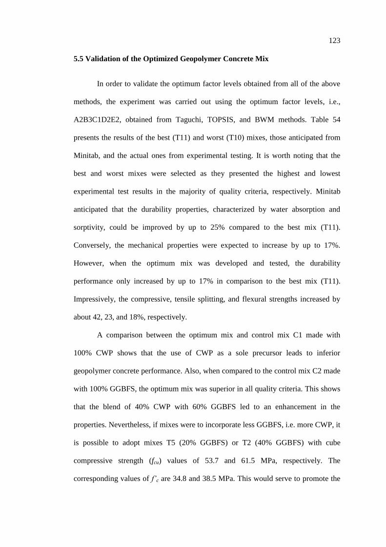
123
5.5 Validation of the Optimized Geopolymer Concrete Mix
In order to validate the optimum factor levels obtained from all of the above
methods, the experiment was carried out using the optimum factor levels, i.e.,
A2B3C1D2E2, obtained from Taguchi, TOPSIS, and BWM methods. Table 54
presents the results of the best (T11) and worst (T10) mixes, those anticipated from
Minitab, and the actual ones from experimental testing. It is worth noting that the
best and worst mixes were selected as they presented the highest and lowest
experimental test results in the majority of quality criteria, respectively. Minitab
anticipated that the durability properties, characterized by water absorption and
sorptivity, could be improved by up to 25% compared to the best mix (T11).
Conversely, the mechanical properties were expected to increase by up to 17%.
However, when the optimum mix was developed and tested, the durability
performance only increased by up to 17% in comparison to the best mix (T11).
Impressively, the compressive, tensile splitting, and flexural strengths increased by
about 42, 23, and 18%, respectively.
A comparison between the optimum mix and control mix C1 made with
100% CWP shows that the use of CWP as a sole precursor leads to inferior
geopolymer concrete performance. Also, when compared to the control mix C2 made
with 100% GGBFS, the optimum mix was superior in all quality criteria. This shows
that the blend of 40% CWP with 60% GGBFS led to an enhancement in the
properties. Nevertheless, if mixes were to incorporate less GGBFS, i.e. more CWP, it
is possible to adopt mixes T5 (20% GGBFS) or T2 (40% GGBFS) with cube
compressive strength (fcu) values of 53.7 and 61.5 MPa, respectively. The
corresponding values of f’c are 34.8 and 38.5 MPa. This would serve to promote the

124
use of CWP as a binder in geopolymer concrete with acceptable performance for
structural applications.
Table 52: Quality criteria values and improvement in optimal mixture design
Property Q1 Q2 Q3 Q4 Q5 Q6 Q7 Q8 Q9
Unit MPa % mm/s0.5
% MPa MPa GPa Ω cm m/s
Best T11 56.6 4.15 0.027 9.27 4.87 3.09 25.9 4266 6469
Worst T10 10.6 7.02 0.047 100 1.64 1.09 3.7 768 2878
Control C1 3.3 8.35 0.055 100 0.8 0.64 1.5 250 2539
Control C2 54.5 4.23 0.029 11.3 4.65 2.98 24.3 3675 5710
Anticipated
Propertya
61.5 3.11 0.02 9.11 5.62 3.62 25.25 4521 6531
Anticipated
Improvement
(%)b
8.7 25.1 25.9 1.7 15.4 17.2 2.5 6 1
Actual
Propertyc
80.3 3.45 0.025 8.98 5.72 3.81 27.4 4652 6745
Actual
Improvement
(%)d
41.9 16.9 7.4 3.1 17.5 23.3 5.8 9 4.3
a The anticipated property is the theoretical value obtained from the optimization methods
b The anticipated improvement is calculated with respect to the best mix T11
c The actual property is the average experimental value of the optimized mix
d The actual improvement is calculated with respect to the best mix T11
125
Chapter 6: Conclusions and Recommendations
6.1 Introduction
The main aim of this study was to develop and evaluate the performance of
geopolymer concrete made with different proportions of CWP and GGBFS. The
viability of using CWP and GGBFS in geopolymer concrete at different ratios to
produce sustainable concrete mixtures was studied in this thesis. This proposed
geopolymer concrete will provide a novel sustainable solution to globally renowned
environmental issues, namely the depletion of natural resources and emission of
carbon dioxide. It will also beneficially recycle industrial by-products in construction
materials and applications rather than wastefully discarding them into landfills and
stockpiles.
The experimental program in this thesis comprised three experimental phases.
As-received CWP, GGBFS, aggregates, and solutions were characterized in the first
phase, such as particle size distribution, moisture content, and specific surface area,
among others, and using various techniques such as SEM and XRD. In the second
phase, the CWP-GGBFS blended geopolymer concrete mixtures were developed
based on Taguchi L16 type-B Orthogonal arrays. Experiments were conducted to
determine the effect of mixture proportions, including binder content, CWP-to-
GGBFS ratio, AAS/binder ratio, SS/SH ratio, and NaOH molarity, on the concrete
properties. These comprise density, compressive strength, modulus of rupture,
splitting tensile strength, modulus of elasticity, ultrasonic pulse velocity, water
absorption, abrasion resistance, bulk electrical resistivity, and sorptivity.
Additionally, the third phase comprised multi-response optimization using the Best

126
Worst Method (BWM) and Technique for Order Preference by Similarity to Ideal
Solution (TOPSIS) based Taguchi methods. Subsequently, verification experiments
were carried out on the proposed optimized mix for validation. The main findings of
this thesis work along with recommendations for future works are outlined hereafter.
6.2 Limitations
The findings of this research work are limited to the types of GGBFS and
CWP employed in this thesis. The coarse and fine aggregates are in the form of
dolomitic limestone and dune sand, respectively, while the alkaline activator
comprised sodium silicate and sodium hydroxide. Variations in the chemical
compositions or physical properties of these binding materials or replacing these
aggregates may result in different outcomes.
6.3 Conclusions
Based on the experimental results presented in this thesis, the following
conclusions can be drawn:
The hardened density of CWP-GGBFS blended geopolymer concrete reached
values up to 2486 kg/m3. It was mainly impacted by the GGBFS replacement
and molarity of the SH solution. Other factors, including binder content,
AAS/binder, and SS/SH seemed to be less impactful. The lowest value was
that of the control mix made with 100% CWP.
A linear regression model was developed to relate the fresh and hardened
density. With a correlation coefficient, R2, of 0.97, it was deemed possible to
predict one density from another with high accuracy.

127
The water absorption was lowest in mixes that had a GGBFS replacement
above 40%, AAS/binder ratio below 0.6, SS/SH ratio below 2, and SH
molarity other than 12. Indeed, the highest absorption was for the control mix
made with 100% CWP. It was apparent that the incorporation of GGBFS into
CWP geopolymer mixes was critical to obtaining a dense matrix with low
absorption capacity. Similar findings were noted for the sorptivity.
The compressive strength was affected by the GGBFS replacement,
AAS/binder, SS/SH, and molarity of SH solution. In fact, respective values in
the ranges of 20-60%, 0.50-0.55, 1.5-2, and 10-14 M led to superior
compressive strength. The highest compressive strength was for mix T11
incorporating 60% GGBFS followed by the control made with 100%
GGBFS. While geopolymer concrete mixes made 80% CWP could reach a
cube compressive strength up to 53 MPa (f’c = 35 MPa), which is sufficient
for most structural applications, cube strengths exceeding 60 MPa (f’c = 39
MPa) require at least 40% GGBFS replacement.
The cube and cylinder compressive strengths of CWP-GGBFS blended
geopolymer concrete were correlated using a linear regression model. With a
high correlation coefficient (R2) of 0.96, it is possible to accurately predict
one strength from the other.
Compression stress-strain curves showed that the replacement of CWP by
GGBFS resulted in a more brittle geopolymeric structure with a lower peak
strain. Nevertheless, the modulus of elasticity was higher. In fact, Ec varied
based on the mixture proportions. A newly-developed multivariable
regression model showed that AAS/binder and SS/SH had a negative impact
on the modulus of elasticity, while binder content, GGBFS replacement, and

128
molarity of SH solution had a positive influence, with the latter being most
significant.
The splitting tensile and flexural strengths of CWP-GGBFS blended
geopolymer concrete followed a similar trend to the 28-day cylinder
compressive strength. Indeed, values of fsp and fr were highest in mixes with
GGBFS replacement, AAS/binder, SS/SH, and molarity of SH solution in the
ranges of 20-60%, 0.50-0.55, 1.5-2, and 10-14 M, respectively. Nevertheless,
it was apparent that the impact of varying the mixture proportions was more
impactful on f’c than fsp and fr.
The abrasion mass loss continuously increased over 500 revolutions for
mixes made with 20% GGBFS replacement. Conversely, mixes with higher
replacements of 40% and above tended to plateau after 300 revolutions. The
values ranged between 9.27 and 100% with the lowest mass losses being
attributed to mixes with the highest compressive strength.
The 28-day cylinder compressive strength of CWP-GGBFS blended
geopolymer concrete was correlated to each of the modulus of elasticity,
flexure strength, splitting tensile strength, and abrasion mass loss. Good
correlations were reported for all regression models with R2 > 0.90 in all
cases. Thus, it is possible to predict these mechanical and durability
properties from the cylinder compressive strength with reasonable accuracy.
Codified equations were generally less accurate in predicting the
performance.
The bulk resistivity of CWP-GGBFS blended geopolymer concrete varied
between 250 and 4266 Ω.cm. Compared to conventional concrete with
similar strength values, the bulk resistivity reported herein is significantly

129
lower, owing to the free ions available in the geopolymeric pore structure.
Yet, they were aligned with the variations shown in the compressive strength.
A correlation model was developed to predict the 28-day compressive
strength from this non-destructive test with reasonable accuracy (R2 = 0.92).
The ultrasonic pulse velocity results indicated that six and four of the
produced mixes were classified to have “good” and “excellent” quality,
respectively. This NDT could also be used to predict the 28-day compressive
strength using a newly-developed linear regression model with reasonable
accuracy (R2 = 0.93).
The ANOVA results showed that the contribution of AAS/binder and
GGBFS replacement on the 28-day cylinder compressive strength were the
highest. The other parameters seemed to be less impactful, with binder
content having the lowest contribution.
The ANOVA of S/N ratios using the Taguchi method for the 28-day cylinder
compressive strength showed that the optimum mix was that with a binder
content, GGBFS replacement percentage, AAS/binder ratio, SS/SH ratio, and
molarity of SH of 450 kg/m3, 60%, 0.50, 1.5, and 10 M, respectively
(A2B3C1D2E2).
The application of the Best-Worst method using nine, five, and two quality
criteria led to the same optimum mix. In fact, it was the same as that
suggested by the Taguchi method to optimize the 28-day cylinder
compressive strength, owing to the strong correlations between the
mechanical properties and f’c. The ANOVA of S/N ratios, considering nine,
five, and two quality criteria, showed that the contribution of the SS/SH and
AAS/binder were the highest. The GGBFS replacement and molarity of SH

130
solution had similar contributions, while the binder content had a limited
contribution (<5%).
The optimum factor levels from TOPSIS-based Taguchi optimization were
found to be A2B3C1D2E2 whether nine, five, or two criteria were
considered. This is similar to the optimum mix determined by Taguchi and
BWM. Considering the nine quality criteria, the ANOVA of S/N ratios of the
TOPSIS method revealed that the contribution of the SS/SH was the highest.
The remaining parameters had similar contributions. For the cases of five and
two quality criteria, the contribution of the binder content increased while
those of the molarity of SH solution and SS/SH decreased.
The optimum factors obtained from Taguchi, BWM, and TOPSIS methods
were validated. The CWP-GGBFS blended geopolymer concrete mix
exhibited a compressive strength of 80.3 MPa, water absorption of 3.45%,
sorptivity of 0.025 mm/s0.5
, abrasion mass loss of 8.98%, flexural strength of
5.72 MPa, splitting tensile strength of 3.81 MPa, modulus of elasticity of 27.4
GPa, bulk resistivity of 4652 Ω.cm, and UPV of 6745 m/s.
6.4 Recommendations for Future Studies
Based on the experimental test results and the above conclusions, a number of
recommendations for future studies in the field of CWP-GGBFS blended
geopolymer concrete are proposed as follows:
Investigate the impact of variant contents of different superplasticizers on
the workability of CWP-GGBFS blended geopolymer concrete.
Examine the structural shear and flexural behaviors of CWP-GGBFS
blended geopolymer concrete.

131
Study the resistance of CWP-GGBFS blended geopolymer concrete to
elevated temperatures, seawater exposure, and acid and sulfate attack.
Evaluate the performance of CWP-GGBFS blended geopolymer concrete
incorporating other waste materials, including recycled aggregates.
Examine the effect of ternary and quaternary mixes incorporating other
industrial by-products on the performance of CWP-GGBFS blended
geopolymer.
Characterize the microstructure of CWP-GGBFS blended geopolymer
concrete.
Perform a lifecycle assessment analysis to verify the feasibility of
utilizing CWP-GGBFS blended geopolymer concrete in structural
applications.

132
References
[1] Afkhami, B., et al., Energy consumption assessment in a cement production
plant. Sustainable Energy Technologies and Assessments, 2015. 10: p. 84-89.
[2] Benhelal, E., et al., Global strategies and potentials to curb CO2 emissions in
cement industry. Journal of Cleaner Production, 2013. 51: p. 142-161.
[3] Herzog, H., et al., Capturing greenhouse gases. Scientific American, 2000.
282, DOI: 10.1038/scientificamerican0200-72
[4] Tans, P. Trends in Atmospheric Carbon Dioxide. 2008.
[5] El-Dieb, A.S., et al., The use of ceramic waste powder (CWP) in making eco-
friendly concretes in ceramic materials - synthesis, characterization,
applications and recycling, D.E. Quesada, Editor. 2018, Intech Open:
London, UK, DOI: 10.5772/intechopen.81842
[6] Pacheco-Torgal, F. and Jalali, S., Reusing ceramic wastes in concrete.
Construction and Building Materials, 2010. 24(5): p. 832-838.
[7] Sun, Z., et al., Synthesis and thermal behavior of geopolymer-type material
from waste ceramic. Construction and Building Materials, 2013. 49: p. 281-
287.
[8] El-Dieb, A.S. and Kanaan, D.M., Ceramic waste powder an alternative
cement replacement – Characterization and evaluation. Sustainable Materials
and Technologies, 2018. 17, https://doi.org/10.1016/j.susmat.2018.e00063
[9] El-Gamal, S.M.A., et al., Ceramic waste as an efficient material for
enhancing the fire resistance and mechanical properties of hardened
Portland cement pastes. Construction and Building Materials, 2017. 154: p.
1062-1078.

133
[10] Mohammadhosseini, H., et al., Enhanced performance of green mortar
comprising high volume of ceramic waste in aggressive environments.
Construction and Building Materials, 2019. 212: p. 607-617.
[11] Kannan, D.M., et al., High performance concrete incorporating ceramic
waste powder as large partial replacement of Portland cement. Construction
and Building Materials, 2017. 144: p. 35-41.
[12] Bignozzi, M.C., and Saccani, A., Ceramic waste as aggregate and
supplementary cementing material: A combined action to contrast alkali
silica reaction (ASR). Cement and Concrete Composites, 2012. 34(10): p.
1141-1148.
[13] Huseien, G.F., et al., Evaluation of alkali-activated mortars containing high
volume waste ceramic powder and fly ash replacing GBFS. Construction and
Building Materials, 2019. 210: p. 78-92.
[14] Katzer, J., Strength performance comparison of mortars made with waste fine
aggregate and ceramic fume. Construction and Building Materials, 2013. 47:
p. 1-6.
[15] Puertas, F., et al., Ceramic wastes as alternative raw materials for Portland
cement clinker production. Cement and Concrete Composites, 2008. 30(9): p.
798-805.
[16] Senthamarai, R.M. and Devadas Manoharan, P., Concrete with ceramic waste
aggregate. Cement and Concrete Composites, 2005. 27(9–10): p. 910-913.
[17] Senthamarai, R.M., et al., Concrete made from ceramic industry waste:
Durability properties. Construction and Building Materials, 2011. 25(5): p.
2413-2419.

134
[18] Guerra, I., et al., Eco-efficient concretes: The effects of using recycled
ceramic material from sanitary installations on the mechanical properties of
concrete. Waste Management, 2009. 29(2): p. 643-646.
[19] Medina, C., et al., Reuse of sanitary ceramic wastes as coarse aggregate in
eco-efficient concretes. Cement and Concrete Composites, 2012. 34(1): p. 48-
54.
[20] Medina, C., et al., Leaching in concretes containing recycled ceramic
aggregate from the sanitary ware industry. Journal of Cleaner Production,
2014. 66: p. 85-91.
[21] Keshavarz, Z. and Mostofinejad, D., Porcelain and red ceramic wastes used
as replacements for coarse aggregate in concrete. Construction and Building
Materials, 2019. 195: p. 218-230.
[22] Anderson, D.J., et al., Mechanical properties of concrete utilising waste
ceramic as coarse aggregate. Construction and Building Materials, 2016.
117: p. 20-28.
[23] Halicka, A., et al., Using ceramic sanitary ware waste as concrete aggregate.
Construction and Building Materials, 2013. 48: p. 295-305.
[24] Heidari, A. and Tavakoli, D., A study of the mechanical properties of ground
ceramic powder concrete incorporating nano-SiO2 particles. Construction
and Building Materials, 2013. 38: p. 255-264.
[25] Zegardło, B , et al., Ultra-high strength concrete made with recycled
aggregate from sanitary ceramic wastes – The method of production and the
interfacial transition zone. Construction and Building Materials, 2016. 122:
p. 736-742.

135
[26] Awoyera, P.O., et al., Green concrete production with ceramic wastes and
laterite. Construction and Building Materials, 2016. 117: p. 29-36.
[27] López, V., et al., Eco-efficient concretes: impact of the use of white ceramic
powder on the mechanical properties of concrete. Biosystems Engineering,
2007. 96(4): p. 559-564.
[28] Abadou, Y., et al., Ceramic waste influence on dune sand mortar
performance. Construction and Building Materials, 2016. 125: p. 703-713.
[29] Huang, B., et al., Laboratory evaluation of incorporating waste ceramic
materials into Portland cement and asphaltic concrete. Construction and
Building Materials, 2009. 23(12): p. 3451-3456.
[30] Torkittikul, P. and Chaipanich, A., Utilization of ceramic waste as fine
aggregate within Portland cement and fly ash concretes. Cement and
Concrete Composites, 2010. 32(6): p. 440-449.
[31] Nayana, A.M. and Rakesh, P., Strength and durability study on cement
mortar with ceramic waste and micro-silica. Materials Today: Proceedings,
2018. 5(11, Part 3): p. 24780-24791.
[32] Jackiewicz-Rek, W., et al., Properties of cement mortars modified with
ceramic waste fillers. Procedia Engineering, 2015. 108: p. 681-687.
[33] Binici, H., Effect of crushed ceramic and basaltic pumice as fine aggregates
on concrete mortars properties. Construction and Building Materials, 2007.
21(6): p. 1191-1197.
[34] Hadi, M.N.S., et al., Design of geopolymer concrete with GGBFS at ambient
curing condition using Taguchi method. Construction and Building Materials,
2017. 140: p. 424-431.

136
[35] Ramujee, K. and PothaRaju, M., Mechanical properties of geopolymer
concrete composites. Materials Today: Proceedings, 2017. 4(2, Part A): p.
2937-2945.
[36] Muttashar, H.L., et al., Self-compacting geopolymer concrete with spend
garnet as sand replacement. Journal of Building Engineering, 2018. 15: p.
85-94.
[37] Valencia-Saavedra, et al., Geopolymeric concretes based on fly ash with high
unburned content. Construction and Building Materials, 2018. 165: p. 697-
706.
[38] Chuah, S., et al., The properties of fly ash based geopolymer mortars made
with dune sand. Materials & Design, 2016. 92: p. 571-578.
[39] Wang, W-C., et al., Study on engineering properties of alkali-activated ladle
furnace slag geopolymer. Construction and Building Materials, 2016. 123: p.
800-805.
[40] Huseien, G.F., et al., Waste ceramic powder incorporated alkali activated
mortars exposed to elevated Temperatures: Performance evaluation.
Construction and Building Materials, 2018. 187: p. 307-317.
[41] Huseien, G.F., et al., Properties of ceramic tile waste based alkali-activated
mortars incorporating GBFS and fly ash. Construction and Building
Materials, 2019. 214: p. 355-368.
[42] El-Hassan, H. and Elkholy, S., Performance evaluation and microstructure
characterization of steel fiber-reinforced alkali-activated slag concrete
incorporating fly ash. Journal of Materials in Civil Engineering, 2019.
31(10): p. 04019223, https://doi.org/10.1061/(ASCE)MT.1943-5533.0002872

137
[43] El-Hassan, H., et al., Influence of different curing regimes on the
performance and microstructure of alkali-activated slag concrete. Journal of
Materials in Civil Engineering, 2018. 30(9): p. 04018230,
https://doi.org/10.1061/(ASCE)MT.1943-5533.0002436
[44] El-Hassan, H., et al., Effect of curing regime on the performance and
microstructure characteristics of alkali-activated slag-fly ash blended
concrete. Journal of Sustainable Cement-Based Materials, 2021,
https://doi.org/10.1080/21650373.2021.1883145
[45] Onoue, K. and Bier, T.A., Optimization of alkali-activated mortar utilizing
ground granulated blast-furnace slag and natural pozzolan from Germany
with the dynamic approach of the Taguchi method. Construction and Building
Materials, 2017. 144: p. 357-372.
[46] Şimşek, B and Uygunoğlu, T., Multi-response optimization of polymer
blended concrete: A TOPSIS based Taguchi application. Construction and
Building Materials, 2016. 117: p. 251-262.
[47] Şimşek, B , Y et al., A TOPSIS-based Taguchi optimization to determine
optimal mixture proportions of the high strength self-compacting concrete.
Chemometrics and Intelligent Laboratory Systems, 2013. 125: p. 18-32.
[48] Sharifi, E., et al., Optimization of high-strength self-consolidating concrete
mix design using an improved Taguchi optimization method. Construction
and Building Materials, 2020. 236: p. 117-547.

138
[49] Elkholy, S. and El-Hassan, H., Mechanical and micro-structure
characterization of steel fiber-reinforced geopolymer concrete. in
Interdependence between Structural Engineering and Construction
Management. 2019. Chicago, IL: ISEC Press,
DOI:10.14455/ISEC.res.2019.109
[50] ASTM, Standard test methods for specific gravity of soil solids by water
pycnometer, in D854. 2014, ASTM International: West Conshohocken, PA.
[51] ASTM, Standard test method for bulk density (“unit weight”) and voids in
aggregate, in C29. 2017, ASTM International: West Conshohocken, PA.
[52] ASTM, Standard test methods for fineness of hydraulic cement by air-
permeability apparatus, in C204. 2017, ASTM International: West
Conshohocken, PA.
[53] ASTM, Standard test method for sieve analysis of fine and coarse
aggregates, in C136. 2014, ASTM International: USA.
[54] Ismail, N. and El-Hassan, H., Development and characterization of fly
ash/slag-blended geopolymer mortar and lightweight concrete. Journal of
Materials in Civil Engineering, 2018. 30(4),
https://doi.org/10.1061/(ASCE)MT.1943-5533.0002209
[55] El-Hassan, H. and Ismail, N., Effect of process parameters on the
performance of fly ash/GGBS blended geopolymer composites. Journal of
Sustainable Cement-Based Materials, 2018. 7(2): p. 122-140.
[56] Ismail, N., et al., Development of a low-cost cement free polymer concrete
using industrial by-products and dune sand. MATEC Web Conf., 2017. 120,
DOI:10.1051/matecconf/201712003005

139
[57] El-Hassan, H., et al., Effect of GGBS and curing temperature on
microstructure characteristics of lightweight geopolymer concrete. MATEC
Web Conf., 2017. 120: p. 03004, DOI.org/10.1051/matecconf/201712003004
[58] Zhang, P., et al., Properties of fresh and hardened fly ash/slag based
geopolymer concrete: A review. Journal of Cleaner Production, 2020. 270,
https://doi.org/10.1016/j.jclepro.2020.122389
[59] Elahi, M.M.A., et al., A review on alkali-activated binders: Materials
composition and fresh properties of concrete. Construction and Building
Materials, 2020. 260, https://doi.org/10.1016/j.conbuildmat.2020.119788.
[60] Mehta, A., et al., Fly ash and ground granulated blast furnace slag-based
alkali-activated concrete: Mechanical, transport and microstructural
properties. Construction and Building Materials, 2020. 257,
https://doi.org/10.1016/j.conbuildmat.2020.119548.
[61] Ismail, I., et al., Modification of phase evolution in alkali-activated blast
furnace slag by the incorporation of fly ash. Cement and Concrete
Composites, 2014. 45: p. 125-135.
[62] ASTM, Standard specification for concrete aggregates, in C33. 2016, ASTM
International: West Conshohocken, PA.
[63] ASTM, Standard test method for relative density (specific gravity) and
absorption of coarse aggregate, in C127. 2015, ASTM International: West
Conshohocken, PA.
[64] ASTM, Standard test method for resistance to degradation of small-size
coarse aggregate by abrasion and impact in the los angeles machine, in
C131. 2014, ASTM International: West Conshohocken, PA.

140
[65] ASTM, Standard test method for soundness of aggregates by use of sodium
sulfate or magnesium sulfate, in C88. 2013, ASTM International: West
Conshohocken, PA.
[66] ASTM, Standard test method for density (unit weight), yield, and air content
(gravimetric) of concrete, in C138. 2017, ASTM International: West
Conshohocken, PA.
[67] ASTM, Standard test method for compressive strength of cylindrical concrete
specimens, in C39. 2015, ASTM: West Conshohocken, PA.
[68] British Standard, Testing hardened concrete - Compressive strength of test
specimens, in BS EN 12390-3. 2009, British Standard: London, UK.
[69] ASTM, Standard test method for static modulus of elasticity and poisson’s
ratio of concrete in compression, in C469. 2014, ASTM International: West
Conshohocken, PA.
[70] ASTM, Standard test method for splitting tensile strength of cylindrical
concrete specimens, in C496. 2011, ASTM: West Conshohocken, PA.
[71] ASTM, Standard test method for flexural strength of concrete (using simple
beam with third-point loading), in C78. 2016, ASTM International: West
Conshohocken, PA.
[72] ASTM, Standard test method for bulk electrical resistivity or bulk
conductivity of concrete, in C1876. 2019, ASTM International: West
Conshohocken, PA.
[73] ASTM, Standard test method for pulse velocity through concrete, in C597.
2016, ASTM: West Conshohocken, PA.
[74] ASTM, Standard test method for density, absorption, and voids in hardened
concrete, in C642. 2013, ASTM International: West Conshohocken, PA.

141
[75] ASTM, Standard test method for measurement of rate of absorption of water
by hydraulic-cement concretes,, in C1585. 2013, ASTM International: West
Conshohocken, PA.
[76] ASTM, Standard test method for determining potential resistance to
degradation of pervious concrete by impact and abrasion, in C1747. 2013,
ASTM International: West Conshohocken, PA.
[77] Brunelli, M. and Rezaei, J., A multiplicative best–worst method for multi-
criteria decision making. Operations Research Letters, 2019. 47(1): p. 12-15.
[78] Martys, N.S. and Ferraris, C.F., Capillary transport in mortars and concrete.
Cement and Concrete Research, 1997. 27(5): p. 747-760.
[79] Saha, S. and Rajasekaran, C., Enhancement of the properties of fly ash based
geopolymer paste by incorporating ground granulated blast furnace slag.
Construction and Building Materials, 2017. 146(Supplement C): p. 615-620.
[80] Bakharev, T., et al., Effect of admixtures on properties of alkali-activated
slag concrete. Cement and Concrete Research, 2000. 30(9): p. 1367-1374.
[81] Aydın, S and Baradan, B., Effect of activator type and content on properties
of alkali-activated slag mortars. Composites Part B: Engineering, 2014. 57:
p. 166-172.
[82] Olivia, M. and Nikraz, H., Properties of fly ash geopolymer concrete
designed by Taguchi method. Materials & Design (1980-2015), 2012. 36: p.
191-198.
[83] ACI Committee 318, Building code requirements for structural concrete and
commentary. 2014, American Concrete Institute: Farmington Hills, Michigan.
[84] ACI Committee 363, State of the art report on high-strength concrete. 1992,
American Concrete Institute: Farmington Hills, MI. p. 364-411.

142
[85] AS3600, Concrete structures. 2009, Standards Australia: Australia. p. 198.
[86] Comité euro-international du béton and Federation International de la
Precontrainte, CEB-FIP Model Code 1990: Design Code. 1993: T. Telford.
[87] Mehta, P.K., and Monteiro, J. P., Concrete microstructure, properties and
material. 2006, New York: McGraw Hill.
[88] Malhotra, V.M. and Carino, N.J., Handbook on nondestructive testing of
concrete. 2nd ed. 1976, Boca Raton, USA: CRC Press.