RESEARCH PAPER

Performance of alternative spatial models in empirical Douglas-firand simulated datasets

Eduardo Pablo Cappa1,2 & Facundo Muñoz3 & Leopoldo Sanchez3

Received: 7 September 2018 /Accepted: 15 April 2019# INRA and Springer-Verlag France SAS, part of Springer Nature 2019

Abstract& Key message Based on an empirical dataset originating from the French Douglas-fir breeding program, we showed thatthe bidimensional autoregressive and the two-dimensional P-spline regression spatial models clearly outperformed theclassical block model, in terms of both goodness of fit and predicting ability. In contrast, the differences between bothspatial models were relatively small. In general, results from simulated data were well in agreement with those fromempirical data.& Context Environmental (and/or non-environmental) global and local spatial trends can lead to biases in the estimation ofgenetic parameters and the prediction of individual additive genetic effects.& Aims The goal of the present research is to compare the performances of the classical a priori block design (block) and twodifferent a posteriori spatial models: a bidimensional first-order autoregressive process (AR) and a bidimensional P-splineregression (splines).& Methods Data from eight trials of the French Douglas-fir breeding program were analyzed using the block, AR, and splinesmodels, and data from 8640 simulated datasets corresponding to 180 different scenarios were also analyzed using the two aposteriori spatial models. For each real and simulated dataset, we compared the fitted models using several performance metrics.& Results There is a substantial gain in accuracy and precision in switching from classical a priori blocks design to any of the twoalternative a posteriori spatial methodologies. However, the differences between AR and splines were relatively small. Simulations,covering a larger though oversimplified hypothetical setting, seemed to support previous empirical findings. Both spatial ap-proaches yielded unbiased estimations of the variance components when they match with the respective simulation data.& Conclusion In practice, both spatial models (i.e., AR and splines) suitably capture spatial variation. It is usually safe to use anyof them. The final choice could be driven solely by operational reasons.

Keywords Global and local spatial trends . Forest genetics trials . Autoregressive residual . Two-dimensional P-splines

Handling Editor: Ricardo Alia

Contributions of the co-authors EPC, FM, and LS conceived anddesigned the research; FM, LS, and EPC planned and carried out thesimulations; EPC and FM analyzed the data; EPC, FM, and LS wrote theoriginal paper; LS supervised the work and coordinated the researchproject.

Electronic supplementary material The online version of this article(https://doi.org/10.1007/s13595-019-0836-9) contains supplementarymaterial, which is available to authorized users.

* Eduardo Pablo Cappacappa.eduardo@inta.gob.ar

1 Bosques Cultivados, Centro de Investigación en Recursos Naturales,Instituto Nacional de Tecnología Agropecuaria (INTA), Instituto deRecursos Biológicos, De Los Reseros y Dr. Nicolás Repetto s/n,1686, Hurlingham, Buenos Aires, Argentina

2 Consejo Nacional de Investigaciones Científicas y Técnicas(CONICET), Buenos Aires, Argentina

3 UMR BioForA, INRA, 45160 Ardon, France

Annals of Forest Science (2019) 76:53 https://doi.org/10.1007/s13595-019-0836-9

1 Introduction

Global and local spatial trends are well known empirically inforestry field trials as a result of environmental factors such asvariations in soil characteristics and land topography. Treebreeders have attempted to account for this environmentalvariability using a priori designs (i.e., by design), includingrandomized complete and incomplete blocks and lattices.However, in most cases, even under the most efficient exper-imental layout, the spatial heterogeneity is conveniently re-vealed at the evaluation stage (Fu et al. 1999). Thus, it is oftennecessary to model such variability a posteriori within themodel of evaluation (i.e., by analysis). Additionally, the spa-tial heterogeneity can also include other non-environmentalfactors such as competition, non-random arrangements of ge-notypes, or any other unexplained variation (Gilmour et al.1997), which could further affect the performance of evalua-tion methods.

Although environmental heterogeneity has been oftenconsidered a nuisance in forest genetic evaluation,where the main goal is the prediction of breedingvalues, ignoring such a source of heterogeneity can leadto biases in the estimation of genetic parameters and theprediction of individual additive genetic effects other-wise known as breeding values (Magnussen 1993,1994). Several a posteriori approaches called Bspatialmodels^ have been developed and widely applied toforest genetic trials in order to account accurately forsite heterogeneity. The impact of small-scale spatial het-erogeneity is accounted for by including a spatially cor-related structure into the model residuals expressed as aKronecker product of first-order autoregressive process-es for rows and columns (Gilmour et al. 1997). Otheralternatives to model the small-scale spatial variabilityuse nearest neighbor techniques (Anekonda and Libby1996; Joyce et al. 2002; Kroon et al. 2008; Gezanet al. 2010) or kriging (Hamann et al. 2002; Zas2006). Large-scale continuous spatial variation has beenmodeled following a variety of approaches, like post-blocking (Ericsson 1997; Lopez et al. 2002; Gezanet al. 2006), the inclusion of spatial coordinatesexpressed as either classification variables such as poly-nomials (Thomson and El-Kassaby 1988; Federer 1998;Saenz-Romero et al. 2001), or smoothing splines(Gilmour et al. 1997; Verbyla et al. 1999). Of theseme thods , a Kronecke r p roduc t o f f i r s t - o rde rautoregressive residual (co)variance structure has be-come commonly used in forest tree breeding. In onedimension (either in rows or in columns), the resultingfirst-order autoregressive structure is equivalent to a

geostatistical model with an exponential covariancefunction. Many forest genetic studies using this spatialmodel approach displayed a consistent reduction in theerror variance and increases in both heritabilities andaccuracies of predicted breeding values with respect tothe a priori model with block design (e.g., Costa e Silvaet al. 2001, Dutkowski et al. 2002, 2006, Ye andJayawickrama 2008). In a first-generation Douglas-firprogeny trial, Ye and Jayawickrama (2008) showed thatthe spatial autoregressive model removed on average 14to 34% of residual variance due to spatial heterogeneity,which resulted in 20% increase in accuracy of breedingvalue prediction with respect to the classical non-spatialmodel.

An alternative approach to model complex patterns of en-vironmental heterogeneity proposed by Cappa and Cantet(2007) is to use a mixed model representation of a two-dimensional P-spline regression (Eilers and Marx, 2003) withspatially structured coefficients. Over a series of studies withforest genetic trials involving large scale (Cappa and Cantet2007), small scale (< 1 ha) (Cappa et al. 2011), and both largeand small scales (Cappa et al. 2015a), the P-splines approachalso displayed a consistent reduction in the residual variancewith respect to the blocks’ model, together with increases inheritability and accuracy of the predicted breeding values ofparents and offspring.

Many forest genetic studies have already compared apriori design models with one of the several a posteriorispatial approaches available. Gezan et al. (2010) com-pared the results from the a priori incomplete blockdesign with those obtained with a model with anautoregressive residual structure, by using simulated da-ta of unrelated genotypes with different surface patterns.The comparison indicated that the incorporation of thisautoregressive structure yielded the highest correlationsbetween the predicted and true treatment effects. Fewstudies, however, have systematically compared severala posteriori methods over a range of trials and paramet-ric scenarios. Saenz-Romero et al. (2001) combinedquadratic polynomials and autoregressive approaches in-to a mixed model to fit simultaneously global and localtrends in a nursery trial. The study showed that thecombination of the two methods was one of the bestanalytical choices. Rodríguez-Álvarez et al. (2018) com-pared the autoregressive approach with a more sophisti-cated spatial model based on splines in an agriculturalcontext.

The goal of the present research is to compare theperformances of alternative approaches to account forvarious patterns of spatial autocorrelation on forest

53 Page 2 of 16 Annals of Forest Science (2019) 76:53

genetic data. Competing methods are the classical apriori block design and two different spatial models: abidimensional separable first-order autoregressive spatialprocess and a bidimensional P-spline regression (hereaf-ter, Bblock,^ BAR,^ and Bsplines^ models, respectively).These are the three most widely used models to accom-modate the spatial heterogeneity in forest genetic trials.The block model is the classical approach to handleenvironmental variation and dates back to the develop-ment of the theory of experimental design almost a cen-tury ago. The AR model is a more modern and flexibleapproach that estimates a nearly continuous surface ofenvironmental effects. Finally, the splines model hasbeen gaining more recognition recently. Besides theirpopularity, they represent three fundamentally differentapproaches to environmental variation. The block modelis based on the aggregation of individuals into groupsthat share similar environments and assume the effect ofthe environment being constant in each group. The ARmodel estimates the correlation between neighboring re-sidual effects. Finally, the splines model belongs to thefamily of kernel smoothers, representing the spatial ef-fect as a linear combination of a set of basis functions.In addition, the present study showcases different mo-dalities for diagnosing competing models, as an addi-tional but important step in the analysis of spatial data.One of the most common tools is the analysis of theresidual semivariograms, which helps to quantify theunaccounted spatial autocorrelation from a given model.Another approach involves cross-validation, a measureof model’s adequacy independent of any model assump-tions (Grondona et al. 1996).

For generality, we based our study on simulated andreal data. Simulated data offer the advantage of cover-ing large parametric ranges that are difficult to find inreal datasets, and allow for a more accurate assessmentof model performance. Our simulated datasets involvedcontrasting spatial patterns generated by both AR andsplines models under different scenarios. Each datasetwas then fitted with AR and splines models and theirrespective performances assessed and compared underseveral criteria. Among the alternative scenarios, thecases of single- and multiple-tree plot designs, andhalf-full-sibs, and clonal genetic structures were studied.We also used data from the French Douglas-fir treeimprovement program to complement simulated scenar-ios and confront the alternative methods to real datasets.These datasets involved a number of mature progenytrials that were established across a range of contrastingsites but yet appropriate for productivity in the context

of the species in France. Precise genetic evaluation atthis stage is of critical importance before selection. Forthis reason, previous analyses based on a priori designwere re-analyzed with these alternative a posteriori spa-tial models (i.e., AR and splines) and the new resultscompared with the previous ones. We discuss the impli-cations of our findings for the French Douglas-fir breed-ing program led by the French National Institute forAgricultural Research (INRA), and wider implicationsfor diagnosis of spatial modeling and genetic evaluationin general.

2 Materials and methods

2.1 Genetic material, mating design, and trialdescription

Data from eight trials of the French Douglas-fir breed-ing program of an appropriated age for genetic evalua-tion were used in the current study (Bastien et al.2013). These trials correspond to progeny tests involv-ing either breeding stock for the renewal of the breedingpopulation (2.707.1, 2.707.3, 2.708.1, and 2.708.3) orprogeny-tested genotypes from first-generation seed or-chards going into genetic thinning (3.704.2, 3.713.1,3.713.1, and 3.713.1). Trials were roughly the sameage, 18 to 21 years after planting, and were chosen tobe representative of the French trial network forDouglas-fir breeding program, accounting for geography,climate, and basic trial disposition. The features of eachof the trials are given in Table 1. The standard designin all eight trials corresponded to a randomized com-plete block setting following a single-tree plot design,with as many blocks as replicates per family. The num-ber of replicates per trial can be found in Table 1.

Two traits, height and diameter at breast height, were mea-sured at 6–8 and 16–20 years, respectively (Table 1).However, not all traits were available for every trial.

2.2 Statistical models of analysis and inference

We compared three individual-tree models of general form:

y ¼ Xβþ Bbþ Zaþ e

with alternative formulations of the spatial random ef-fect Bb: block, AR, and splines. These three models

Annals of Forest Science (2019) 76:53 Page 3 of 16 53

were evaluated for each combination of site and trait inthe Douglas-fir dataset. Although genetic evaluation isgenerally conducted with multiple-trait and multiple-sitemodels, splitting data analyses in this way was justifiedby the need of collecting a broad spectrum of spatialpatterns. The vector y contains the phenotypic data, andall three models included a fixed effect of provenance(β , genetic group) to account for different sub-population means. A set of genetic (a) and residual (e)random effects were also considered in all models. Theformer was a normally distributed random additive ge-netic effect (breeding values) with (co)variance matrixAσ2

a, where A is the additive relationship matrix among

all trees (Henderson 1984), and σ2a is the additive ge-

netic variance. The residuals were independently distrib-uted with mean 0 and residual variance σ2

e . X and Z arethe incidence matrices relating the observations (y) tothe model effects β and a.

The spatial random effect was modeled differently inthe three alternative models. For the block model, Bwas the incidence matrix for blocks and b was a nor-mally distributed random effect with mean 0 and vari-ance σ2

s . The AR model considers b a random effect at

individual level with a covariance structure σ2s

AR1 ρrowð Þ⨂AR1 ρcolð Þ½ � given by the Kronecker productof first-order autoregressive processes AR1(ρ.) in therows (row) and the columns (col) with spatial varianceparameter σ2

s , while B is a permutation matrix to sortobservations by columns within rows (Gilmour et al.1997) . Fina l ly, the spl ines model f i t s a two-dimensional surface built as a tensor product of cubicB-splines basis (Eilers and Marx 2003). The matrix Bcontains the two-dimensional B-splines basis evaluatedin the corresponding row and column for each tree,while the vector of regression coefficients b is normallydistributed with mean 0 and covariance matrix Uσ2

s ,

where U is a fixed spatial structure and σ2s is the spatial

variance parameter. A more detailed explanation of thetwo-dimensional surface and the covariance structureused in this work can be found in Cappa and Cantet(2007). Note that the three formulations (block, AR, andsplines) are mutually exclusive. In particular, the ARand splines models do not include the effect of theblocks.

In order to make the alternative parameters of spatialvariance comparable, we scaled the covariance matrices

so that σ2s represented exactly the characteristic marginal

variance of the spatial effect (Sørbye and Rue 2014).

Table1

Designandphenotypicinform

ationacross

theeightD

ouglas-firprogenytrials

Site

2.707.1

2.707.3

2.708.1

2.708.3

3.704.2

2.713.1

2.713.2

2.713.3

No.of

treeswith

records

5434

6248

6709

8977

2759

3976

3458

1459

Parentsnumber

183

198

221

235

68134

117

66Family

number

OPa

183

198

219

228

6895

7829

FSb|

––

68

–38

3031

No.of

provenances

79

67

–6

88

Replicate(blocks)

8888

100

101

9153

4034

Row

196

120

234

164

5563

9079

Colum

n140

153

83109

74172

9751

Spacing(m

)3×3

3.6×2.75

3×3

4×2.5

3.5×3

3×3

3.5×3

2.5×3.5

Age

atheight

assessment

87

78

87

–6

Age

atdiam

eteratbreastheight

assessment

19–

––

2016

1616

Heightm

ean(m

m)(and

SDc )

413.0(123.4)

405.8(89.8)

416.4(105.9)

572.4(97.1)

443.1(99.4)

495.9(109.3)

–345.7(96.5)

Diameter

atbreastheight

(cm)(and

SD)

415.7(155.8)

––

–636.3(161.9)

486.5(130.0)

530.2(106.0)

449.9(153.9)

Altitude

(ma.s.l.)

330

700

425

720

550

500

710

650

Slope(%

)5–10

1010

108

05–30

2–20

Meanannualprecipitatio

n(m

m)

1100

1440

900

1140

–1200

1300

1100

aOP:o

pen-pollinatedfamilies,b

FS:full-sibfamilies,c

SD:standarddeviation

53 Page 4 of 16 Annals of Forest Science (2019) 76:53

Residual maximum likelihood (REML, Patterson andThompson 1971) was used to estimate the variancecomponents for the random effects in the three spatialmodels described previously, by using the functionremlf90 in the R-package breedR (Muñoz andSanchez, 2015), which is based on the programsREMLF90 and AIREMLF90 of the BLUPF90 library(Misztal 1999). While REML90 uses the Bexpectationmaximization^ algorithm for the variance component es-timation, AIREMLF90 is based on the Baverageinformation^ approach. The former is slower but morerobust to initial values and was used for the more com-plex splines models, while the latter was used for theAR models.

The autocorrelation parameters in the AR models andthe number of row and column knots in the splinesmodels, respectively, were estimated by a grid-searchapproach that fits the model using several combinationsof these values and selects the one with highest log-likelihood. Specifically, for the empirical Douglas-fir da-ta, we used a two-step procedure for AR, initially fittingthe models on a coarse grid with all combinations ofthe values (− 0.8, − 0.2, 0.2, 0.8) for the autoregressiveparameters in each direction. A refined grid of the samesize around the previous best combination was used inthe second step, considering a variation of roughly 20%at each side in each dimension in the logit scale. Forthe spline models, the initial number of knots in eachdimension is a power function of the size of the fieldgiven as a default by breedR. We tested all the

combinations of five values around this initial value ineach dimension, similarly to AR. As a result, searchprocess for the empirical Douglas-fir data assumed anisot-ropy for the AR and splines models; i.e., differentautoregressive parameters and number of knots were fittedin row and column directions.

Standard errors for estimated variances and functions ofvariances (i.e., heritabilities, see equation below) were calcu-lated via Monte Carlo (Manly 1991). This implied samplingrandom realizations of datasets from the corresponding ana-lytical models and estimated variance components.

2.3 Model comparison and diagnosticsfor the empirical Douglas-fir datasets

We compared the predictive ability of the fitted modelswith the Akaike information criterion (AIC, Akaike1974), which is an approximation of the average out-of-sample deviance based on the marginal likelihood. Asmaller AIC value indicates a better trade-off betweengoodness of fit and parsimony.

In addition, a 12-fold cross-validation was conducted.Each dataset was subdivided into 12 equally sized inde-pendent samples. Each of the samples was used forvalidation after fitting the model. The predicting abilitywas obtained as the Pearson correlation between ob-served phenotypes and fitted values. A complementarymeasure of the prediction quality was obtained as theroot mean square error (RMSE) of the fitted values.

Fig. 1 Empirical semivariograms of residuals from the bidimensionalseparable first-order autoregressive (AR) and bidimensional spline re-gression (splines) models fitted to a simulated dataset with a high-

variance short-ranged AR spatial effect under a single-tree plot structure.The horizontal (darker) lines are the estimated values of the residualvariances for a true value of 1

Annals of Forest Science (2019) 76:53 Page 5 of 16 53

Single-site narrow-sense individual heritability h2

� �was

estimated as h2 ¼ σ2

a= σ2a þ σ2

e

� �, where σ2

a is the estimated

additive genetic variance, and σ2e is the estimated resid-

ual variance. We explicitly excluded the spatial variancefrom the denominator in order to get comparable esti-mates of heritability across sites. This simple definitionof heritability does not adhere to the standard quantita-tive genetics assumptions (Cullis et al. 2006), and sothis measure should only be interpreted as a descriptivemeasure of precision (or ability) to detect additive ge-netic differences among the three models studied.

Further model comparison was provided by the predictiveaccuracy of breeding values, computed as:

r ¼ffiffiffiffiffiffiffiffiffiffiffiffiffi1−SE2

σ2a

vuut

where SE stands for the standard error of predictedbreeding values using the Bbest linear unbiasedpredictors^ (BLUPs) of parents and offspring. Finally,Spearman correlations between the best 10% candidatebreeding values obtained by any two alternative modelswere also calculated, in order to check whether theranking of breeding values differed between alternativesand therefore selection decisions were impacted by thechoice of the model.

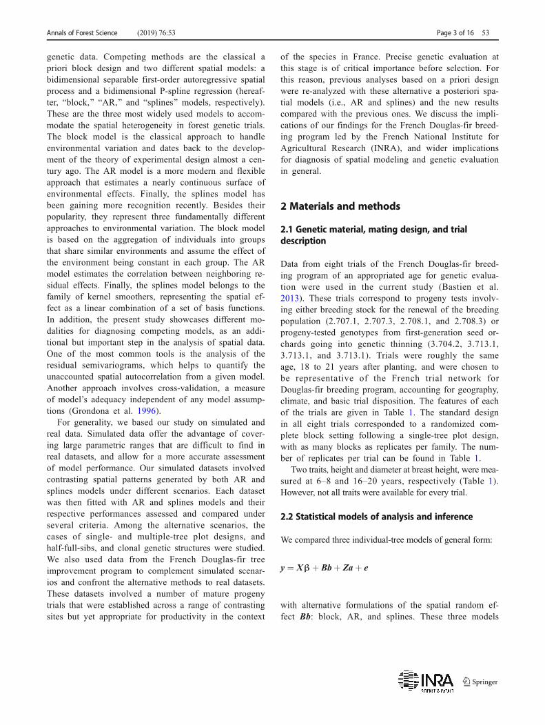
We also computed the empirical semivariogram ofresiduals as a standard model diagnostics tool. The iso-tropic semivariogram represents the half-average varia-tion in pairwise residual differences as a function of thedistance (Cressie 1993). Since the synthetic residualswere simulated independently and identically distributed,a logical expectation is that the empirical semivariogramof the residuals from a model properly accounting forall relevant effects will be approximately constant at theestimated residual variance. Thus, it might be disturbingto obtain empirical residual semivariograms such asthose shown in Fig. 1 after fitting an AR or splinesmodel to an ideal, simulated dataset.

We have seen this pattern emerging often frommodels fitted to real datasets as well (e.g., progeny trial3.704.2; see Fig. 2b), most noticeably with AR spatialmodels. Specifically, the two challenging aspects are:

1. a discrepancy between the variance of the empirical resid-uals and the estimated residual variance, and

2. a remarkable non-flat slope in the first few lags.

Such behavior could lead to thinking that there re-mains some unaccounted structure in the residuals, orthat the spatial effect is overfitting the observations.To assess this, we devised two metrics for quantifyingthe extent of these effects in the simulation experiment(see Section 2.5). For each fitted model, we measuredthe discrepancy between the empirical and estimatedresidual variances (i.e., empirical vs. estimated differ-ences; RV_disc) and the slope of the empiricalsemivariogram of residuals at distance 0 (vgslope).

2.4 Selection of representative trials accordingto spatial patterns

Twelve site-trait combinations from height differenceprogeny trials were analyzed in order to assess the pat-terns of environmental heterogeneity. We examined thespatial distribution of residuals (heat map) and their iso-tropic empirical semivariograms from a model withfixed genetic groups whenever present and individual-tree level additive genetic effects (breeding values).

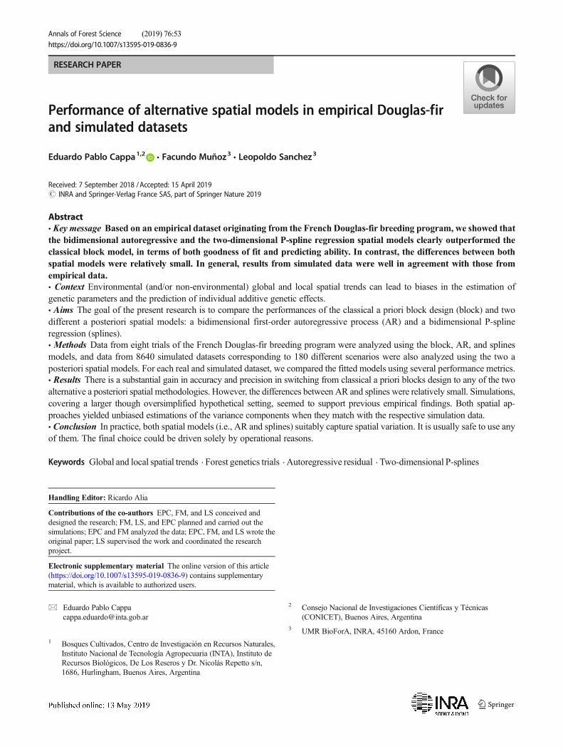
Although all cases were used for comparing the per-formance of the different spatial models, only three ofthem were used as representative cases of the differentspatial pattern scenarios (Fig. 2) for further illustrationin Section 3. The first selected trial (2.708.3, height) isa typical case exhibiting large-scale variation in twodimensions, with a heat map displaying large patchesof similar residuals and a semivariogram with a cleartrend of increasing variation with the distance betweentrees. A trial with mostly short-scale variation is shownin the next panel (2.707.1, height) , where thesemivariogram depicts a rapid change in variation atclose distances with a leveling out at medium distances.The heat map displayed smaller aggregates of similartones than in the previous case. Finally, the last selectedtrial (3.704.2, diameter) displays a very short-scale spatialpattern, with the heat map showing antagonistic residualsin neighboring cells, and a semivariogram with no generaltrend but at the very short range.

Fig. 2 Heat maps (a) and isotropic empirical semivariograms (b)from the residuals of a basic genetic model not accounting forspatial autocorrelation, for three contrasting cases of the eightDouglas-fir progeny trials b

53 Page 6 of 16 Annals of Forest Science (2019) 76:53

0

30

60

90

0 50 100 150

Rows

Columns

−200

0

200

Residuals

3500

4000

4500

5000

5500

0 20 40

distance

variogram

0

50

100

150

0 50 100 150 200

Rows

Columns

−200

0

200

Residuals

a

10000

12500

15000

17500

0 20 40 60 80

distance

variogram

b

0

20

40

60

80

0 20 40

Rows

Columns

−200

0

200

Residuals

13000

13500

14000

0 10 20 30

distance

variogram

Annals of Forest Science (2019) 76:53 Page 7 of 16 53

2.5 Performance assessment of AR and splinesapproaches under simulated scenarios

We designed an extensive simulation experiment where a num-ber of datasets were sampled under several alternative scenarios.We fitted AR and splines models to each dataset and comparedtheir relative performance according to a few selected measures.

Specifically, we simulated 180 datasets of dimension 70 ×70 individuals in each of the 12 scenarios which arise from thecombination of the following:

& generating model: AR and splines& range: short and long& variance ratio of spatial and residual variances: low, me-

dium, and high

Given that the environmental spatial variation may interactwith other non-environmental factors like additive genetic resem-blance between neighbors or plot structure and this interactioncan affect differently the performance of alternative spatialmodeling, we simulated four additional scenarios involving

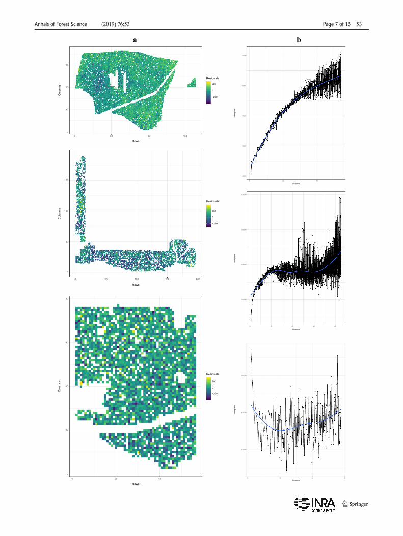
Fig. 3 Random realizations ofexamples of simulated spatialpatterns with the bidimensionalseparable first-orderautoregressive (AR) andbidimensional spline regression(splines) models at short and longspatial ranges

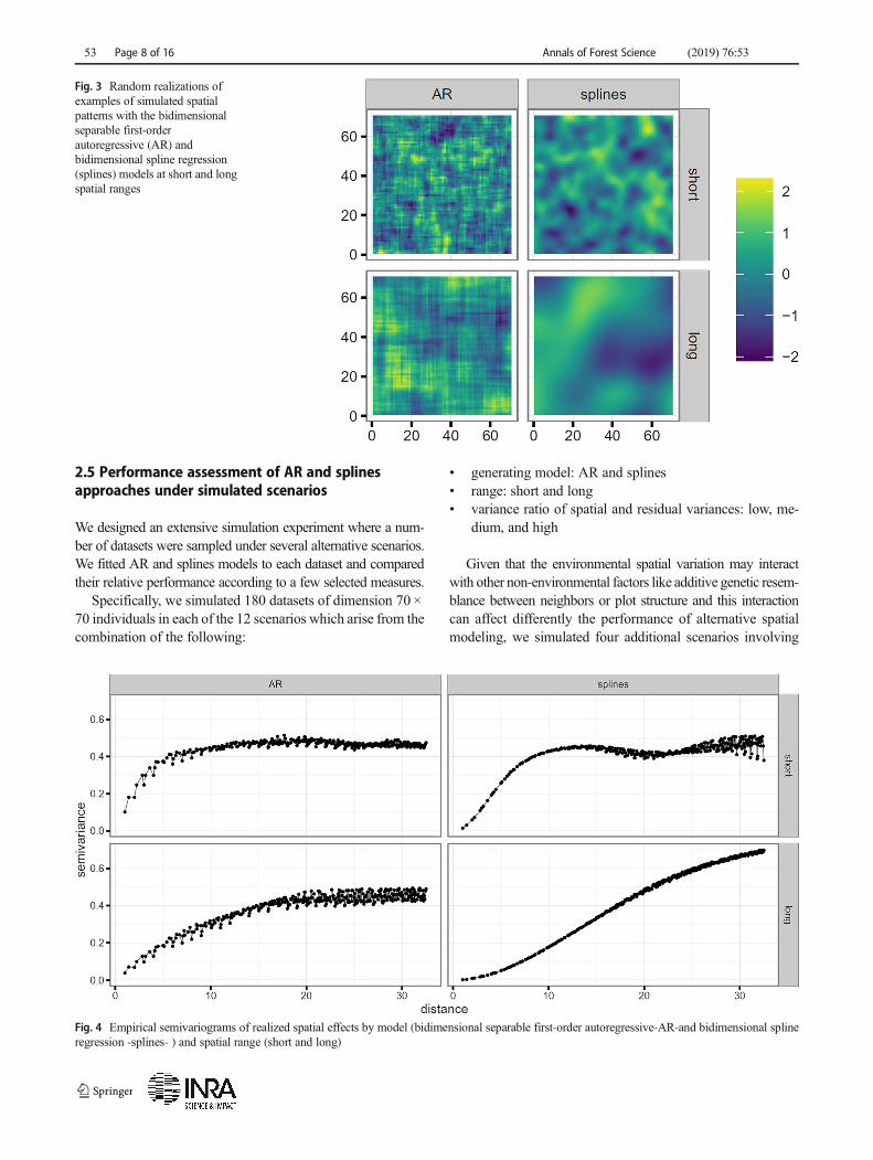
Fig. 4 Empirical semivariograms of realized spatial effects by model (bidimensional separable first-order autoregressive-AR-and bidimensional splineregression -splines- ) and spatial range (short and long)

53 Page 8 of 16 Annals of Forest Science (2019) 76:53

combinations of plot design and within-plot genetic relatedness.The basic scenario was a single-tree plot design (STP) with aGaussian residual variance of 1. No genetic effects were simu-lated in this scenario, since their effect on the estimation of thespatial component would be indistinguishable from the residualsdue to the stochastic independence. Three other alternative sce-narios with multiple-tree plot designs (MTP) of seven trees inline plots differed in their within-plot genetic composition, withclonal, full-sib, and half-sib family structures with independentprogenitors. The STP designs were completely randomized,while the MTP designs were arranged into 10 bands of random-ized line plots with seven individuals each (see SupplementaryFig. S1). For the MTP designs, we assumed an additive geneticvariance of half the residual variance (1/3 and 2/3 respectively),keeping the total at 1 for comparability, and simulated breedingvalues according to the specific family structure. We rescaled thegenetic and residual effects to keep the total variance comparableto that of the STP design.

A short (long) range was simulated with an autocorrelationparameter of 0.80 (0.93) for the AR model and 20 (7) internalknots for the splines model. In all cases, the same parameter wasused for both the row and column directions. The specific valueswere selected to produce spatial patterns with qualitatively dif-ferent ranges of approximately equivalent extent across models.

Figure 3 shows four random realizations of spatial patterns bymodel and range (more examples in Supplementary Fig. S2).

The differences in perceived smoothness between the spatialpatterns from AR and splines are intrinsic to the nature of thesemodels. Specifically, this feature is caused by a fundamentaldifference in the curvature of the semivariogram at 0 (e.g., seeCressie 1993, p. 60). Figure 4 displays the corresponding empir-ical semivariograms for the realized spatial patterns in Fig. 3 (andSupplementary Fig. S3, the corresponding empiricalsemivariograms for the realized spatial patterns inSupplementary Fig. S2).

The categories of the ratio of the spatial effect variance (σ2s )

with respect to the residual variance (σ2e ) (i.e., σ2

s=σ2e ) were

0.0625, 0.25, and 0.5 for low, medium, and high, respectively.The R code used for simulating the entire datasets used in thisstudy is given as an Electronic Supplementary Material(Supplementary R_code S1). Additionally, an R code to generatea reduced simulation studymimicking the entire datasets is givenalso as an Electronic Supplementary Material (SupplementaryR_code S2).

Each of the resulting 180 × 12 × 4 = 8640 datasets was fittedwith both AR and splines models using a grid search for theirrespective parameters (i.e., autocorrelation parameter and

Table 2 Akaike informationcriterion (AIC), estimates ofvariance components (Genetics,Spatial, Residual), heritabilities(Heritability), and average of thecorrelation coefficients and rootmean square errors (RMSE) fromthe cross-validation analyses foreach of the three spatial mixedmodels studied (see text formodels’ abbreviations). Standarderrors are in brackets. The corre-sponding traits analyzed are totalheight for sites 2.708.3 and2.707.1, and diameter for site3.704.2. The lowest AIC andRMSE values, and highest corre-lations values are highlighted initalics

Trial Modela

block AR splines

2.708.3 AIC 104,886 104,454 104,523

Genetic 2507 (172) 2484 (182) 2514 (173)

Spatial 1889 (320) 1786 (172) 1649 (341)

Residual 4625 (107) 4089 (114) 4359 (111)

Heritability 0.35 (0.02) 0.38 (0.002) 0.37 (0.02)

Correlation coefficients 0.54 (0.04) 0.57 (0.03) 0.56 (0.03)

RMSE 23.65 (1.09) 23.1 (1.06) 23.22 (1.03)

2.707.1 AIC 64,179 63,722 63,905

Genetic 1723 (180) 1882 (224) 1770 (217)

Spatial 2050 (403) 4804 (378) 4693 (890)

Residual 11,353 (262) 7998 (163) 10,430 (292)

Heritability 0.13 (0.01) 0.19 (0.02) 0.15 (0.02)

Correlation coefficients 0.38 (0.03) 0.49 (0.03) 0.44 (0.04)

RMSE 33.02 (1.21) 31.07 (1.15) 32.03 (1.24)

3.704.2 AIC 33,830 33,799 33,798

Genetic 7833 (971) 7719 (978) 7731 (1170)

Spatial 286 (137) 907 (354) 578 (268)

Residual 18,155 (799) 18,060 (839) 18,070 (824)

Heritability 0.30 (0.03) 0.30 (0.03) 0.30 (0.04)

Correlation coefficients 0.24 (0.07) 0.26 (0.07) 0.27 (0.07)

RMSE 45.38 (1.91) 45.07 (2.04) 45.05 (2.08)

a block: block design model, AR: bidimensional separable first-order autoregressive model, splines:bidimensional spline regression model

Annals of Forest Science (2019) 76:53 Page 9 of 16 53

number of knots, respectively). The search process assumed isot-ropy (i.e., same parameter value in row and column directions)and fitted seven different values around the true simulated pa-rameter value. The specific values for ρ were defined in a logitscale as logit(ρ0) + (k − 4)/2, k= 1,… , 7, where ρ0 is the value ofthe autocorrelation parameter used for simulation. The specificvalues for the number of knots were defined as exp(log(k0− 2) +(k− 4)/6 + 2), k = 1,… , 7, where k0 is the number of knots usedfor simulation. The resulting values were rounded to two andzero decimal places, respectively. These somewhat arbitraryscales were designed to produce approximately uniformly dis-tributed values in qualitative terms, since, for example, a 0.05increase in correlation from 0.5 has a very different relevancethan from 0.9. The model with the highest likelihood was select-ed as the outcome of the grid-search processes for theautoregressive and knots parameters.

In summary, for each approach (i.e., AR or splines), wefitted seven models to each of the 8640 datasets, which result-ed in more than 120K model fits.

For each dataset and approach, we calculated the followingperformance metrics:

& AIC: Akaike Information Criterion, see above& RMSE: root mean square error of prediction of the expect-

ed phenotype

& RVRD: residual variance relative deviation, i.e., σ2e−σ2eσ2e

& SCor: correlation between predicted and true spatial ef-fects based on the simulations

& SVRD: spatial variance relative deviation, i.e., σ2s−σ2sσ2s

Note that AIC and RMSE are always positive, and lowervalues are better. For RVRD and SVRD, values closer to 0 arepreferable, while SCor ranges between 0 and 1, and higher valuesare superior.

Finally, in order to compare the relative performances of theAR and splines approaches, we computed the differences be-tween the absolute values of their metrics (|mSplines| − |mAR|) foreach simulated dataset. This resulted in a Monte Carlo

approximation (with 8640 samples coming from the 180 differ-ent scenarios) of the sampling distribution of these relative-performance metrics where positive (negative) values favor theAR (splines) approach, except for SCor where this relationship isreversed.

Data availability The datasets generated and analyzed duringthe current study are available in the Zenodo repository(Cappa et al. 2019) at https://doi.org/10.5281/zenodo.2629151.

3 Results

3.1 Results from Douglas-fir case studies

Only one of the 12 traits by site combinations resulted in theblock model being the best performing analytical method. Wepresent the measures of model comparison for the three repre-sentative case studies in Table 2. The equivalent measurementsfor the rest of the trial by trait combinations are shown inSupplementary Table S1. According to AIC, the block modelresulted in the worst fit (i.e., highest AIC), while AR yieldedthe lowest AICs for the cases with large- and short-scale envi-ronmental heterogeneity (2.708.3 and 2.707.1, respectively). Forthe case with very-short-scale environmental heterogeneity(3.704.2), splines gave the best fit although differences were verysmall compared to AR (33,798 versus 33,799, respectively).Both AR and splines yielded smaller residual variance estimatesthan the block model, which resulted ultimately in higher herita-bilities. Measures of predictive ability from cross-validation re-vealed a similar picture of advantages for AR and splines overthe block model (correlation coefficient and RMSE in Table 2).In general, differences between the two best fitting models (ARand splines) were more important when environmental variationwas at short scale than when compared at larger scales, with ARoutperforming splines in terms of AIC and predicting ability.

Apart from fitting quality and heritability increase, accuracy ofbreeding values and eventual change in candidate ranking be-tween models are also of concern for the breeder. Table 3 shows

Table 3 Accuracy of prediction of breeding values from the blockdesign (block), bidimensional separable first-order autoregressive (AR)and bidimensional spline regression (splines) models, and Spearman

correlations coefficients between predicted breeding values of the 10%best candidates for all pairs of models. The corresponding traits analyzedare total height for sites 2.708.3 and 2.707.1, and diameter for site 3.704.2

Trail Accuracy of breeding values Spearman correlation of breeding values

block AR splines block/AR block/splines splines/AR

Parents Offspring Parents Offspring Parents Offspring Parents Offspring Parents Offspring Parents Offspring

2.708.3 0.87 0.66 0.88 0.67 0.88 0.67 0.95 0.83 0.95 0.86 0.96 0.93

2.707.1 0.70 0.47 0.73 0.51 0.71 0.49 0.81 0.74 0.93 0.88 0.90 0.83

3.704.2 0.86 0.63 0.86 0.63 0.86 0.63 0.96 0.95 0.96 0.95 1.00 1.00

53 Page 10 of 16 Annals of Forest Science (2019) 76:53

some statistics concerning resulting breeding values from thethreemodels. As expected, parents reached higher accuracies thanoffspring, and accuracies increased with heritabilities. There wereno clear differences between AR and splines models for accura-cies, except for the short-scale environmental variation case study,for which AR model presented slightly higher accuracies. Blockmodel accuracies were similar or lower than those of AR andsplines models. However, we observed some changes in rankingof best 10% candidates, which were particularly important be-tween block and AR models, presumably because the formertakes mostly account for large-scale environmental variation only.

3.2 Results from simulated scenarios

Figure 5 shows a summary of the sampling distributions of theconsidered performance metrics by fitted model, spatial range,and plot structure. For ease of interpretation, we removed somescenarios that did not add any further insight. Specifically, wekept only the scenarios with highest ratio of spatial to residualvariances, which displayed the same patterns than lower ratiosbut at a higher scale. Furthermore, we show only STP and half-sib MTP designs, since they behave very similar to clone-MTPand full-sib MTP designs, respectively. The full version of theFig. 5, for all scenarios and mating designs with two additionalmetrics considered later, is available in Supplementary Fig. S4.

From Fig. 5, we can confirm some expected results concerningthe differences among scenarios. For instance, that STP designsgenerally yielded more accurate predictions (most clearly interms of RMSE) than MTP, and that MTP designs had largersampling variability (e.g., standard error), notably in the estima-tion of the residual variance. In general, long-ranged spatial ef-fects were easier to fit, and spline-generated spatial effects werealso more easily recovered than AR counterparts. Furthermore,both approaches yielded unbiased estimations of the variancecomponents when they matched the generating spatial model(i.e., simulated model = fitted model; outermost couple of pointsin each panel). Conversely, both approaches are biased in thenon-matching context. It is important to note that the relevantcomparison here is that between fitted models, rather than thatbetween generating models. These latter were simply two alter-native ways of generating a Breality,^ the spatial heterogeneity,for which the experimenter has no clue of its nature.

The relative performances of the splines and AR approachesunder these settings are more accurately assessed from Fig. 6,which displays the differences in absolute value between thesplines and AR metrics by spatial range, simulated model, andplot structure. The distributions over the BAR^ column tended tobe concentrated further away from 0 (meaning larger differencesbetween splines and ARmetrics) than their corresponding coun-terparts over the Bsplines^ column, and this happened for most

Fig. 5 Median and 90% centralquantile of sampling distributionof metrics (root mean squarederror of prediction of the expectedphenotype -RMSE-; residualvariance relative deviation-RVRD- ; correlation betweenpredicted and true simulatedspatial effects -Scor-; and spatialvariance relative deviation-SVRD-) by fitted model(bidimensional separable first-order autoregressive -AR- andbidimensional spline regression-splines-), spatial range (short andlong), and plot structure (design,single-tree plot -STP- andmultiple-tree plot -MTP-)

Annals of Forest Science (2019) 76:53 Page 11 of 16 53

metrics except SVRD at long range which showed the contrary.For example, with spline-generated data, the AR approach isalmost as good as the splines when it comes to estimating theresidual variance, or in terms of correlation between simulatedand predicted spatial effect. There is a more remarkable differ-ence in these metrics in favor of AR when the spatial effect isgenerated by an AR model. We can conclude that even if thedifferences in performance are relatively small with respect to thetarget values, it is easier for the AR approach to fit spline-generated data than the converse. This is particularly true undera scenario of long-ranged spatial effect and STP structure (e.g., interms of RMSE). Under MTP structure, however, the RMSEincreases dramatically for both approaches and the advantageof the AR over splines vanishes almost completely.

Figure 7 displays the marginal distributions of thesemivariogram metrics residual variance discrepancy (RV_disc)and semivariogram slope (vgslope) by (simplified) scenario, de-sign, and approach. Note how the discrepancy between the em-pirical and estimated residual variance is most important underMTP designs, where there is the additional confounding of thespatialized genetic arrangement. For STP designs on the otherhand, the discrepancy is more important for short- rather than forlong-ranged spatial effects, and for the AR than for the splinesapproach, due to the weaker partial pooling. The slope of theempirical semivariogram is systematically negative, except for

the case where the data were simulated with a long-ranged ARspatial process and fitted with a splines approach. This is certain-ly due to unaccounted autocorrelation at a shorter scale, andreflects the mismatch in the covariance model. Otherwise, forthe AR approach under STP structure at short-ranged spatialscale, the negative slope is remarkably steeper than for the splinesapproach, both for AR- or splines-simulated data. This is likely aside effect of the increased correlation between spatial and resid-ual BLUPs. It is not the semivariogram peak which is taller butthe empirical variance which is lower. This can be seen from thenegative correlations between these two metrics for the non-matching cases in Supplementary Fig. S5. From the same Fig.S5, we can see that neither the empirical discrepancy with theestimated residual variance (RV_disc) nor the semivariogramslope (vgslope) is associated with any other metric. This suggeststhat the discrepancy and slope are not signs of over- or under-fitting but a generally expected outcome. Moreover, the fact thatthe AR approach usually displays a steeper slope than splinesdoes not hamper its predictive ability.

4 Discussion

In genetic evaluation and quantitative genetic analyses in for-est trees, environmental heterogeneity is of relevance given

Fig. 6 Median and 90% centralconfidence interval of differencesbetween the bidimensional splineregression (splines) andbidimensional separable first-order autoregressive (AR) abso-lute metrics (i.e., |mSplines| − |mAR|for m equal to root mean squareerror of prediction of the expectedphenotype -RMSE-; residual var-iance relative deviation -RVRD-;correlation between predicted andtrue simulated spatial effects-Scor-; and spatial variance rela-tive deviation -SVRD-) by spatialrange (short and long) and plotstructure (design, single-tree plot-STP- and multiple-tree plot-MTP-). Positive (negative)values indicate a betterperformance by AR (splines),except for SCor where therelationship is the reverse

53 Page 12 of 16 Annals of Forest Science (2019) 76:53

that trials usually comprise large areas often established inmarginal heterogeneous lands, which in turn can exacerbate themagnitude of environmental effects and the need to account pre-cisely for them in the evaluation process. In the era of genome-driven accuracy, we should not forget that environmental termsalso need to be assessed with precision in the populations usedfor calibration, in order to be able to split precisely genetic andenvironmental effects. In this study, we compared one of themost common and classical methods to account for environmen-tal heterogeneity in experimental trials, the blockmodel, which isan a priori method based on design, with two alternatives that arebased on a posteriori analyses using an empirical Douglas fir dataand the a posteriori AR and splines models under different sim-ulated scenarios. Of these latter methods, the ARmodel is one ofthe most popular methods in the spatial literature in forest andcrop evaluation (e.g., Qiao et al. 2000; Smith et al. 2001; Costa eSilva et al. 2001; Dutkowski et al. 2006). P-splines represents amethodologically distinct approach which is considered suitableto fitting trends over large scales than those usually associated toAR models.

We found that a posteriori analyses byAR and splines modelsclearly outperformed the blockmodel. This was the case across aseries of 11 out of the 12 traits by site combinations comprisingeight sites from the Douglas fir genetic evaluation program thatwere used in the present study. Similar outcomes have been

found in previous works involving forest genetic trials, whencomparing a block model to AR (Costa e Silva et al. 2001;Dutkowski et al. 2006; Ye and Jayawickrama 2008) and splines(Cappa et al. 2011 and Cappa et al., 2015a) models. Other aposteriori approaches for spatial modeling showed also improve-ment of estimates of genetic parameters and breeding values overstandard designs, like kriging (Hamann et al. 2002, Zas 2006),and nearest neighbor techniques (Anekonda and Libby 1996,Joyce et al. 2002). In summary, there is a considerable amountof work, of which we referenced just a few studies, all showingthe benefits of a posteriori spatial analyses over classical a prioridesign-based approaches. However, there is a lack of compari-sons between some of the best a posteriori methods.

This study presents one of the first comparisons between twomethodologically distinct a posteriori methods by using bothempirical and simulated data. Our empirical results revealed thatdifferences between AR and splines models in terms of fittingand predicting ability, although in absolute terms favorable to theformer, were relatively small or difficult to discernwhen account-ing for replicate variation in the cross-validation analysis. Theseresults are consistent with those obtained from Velazco et al.(2017) where the performance of the splines model was equiva-lent to the AR model when considering the improvement in theprecision and the predictions of genetic values, even though theyconsidered anisotropic models and a different covariance

Fig. 7 Median and 90% centralquantile of sampling distributionof variogram metrics (empiricaland estimated residual variancesdifferences -RV_disc- and slopeof the empirical semivariogram ofresiduals at distance 0 -vgslope-)by fitted model (bidimensionalseparable first-orderautoregressive -AR- andbidimensional spline regression-splines-), spatial range (short andlong), and plot structure (design,single-tree plot -STP- andmultiple-tree plot -MTP-)

Annals of Forest Science (2019) 76:53 Page 13 of 16 53

structure in the splines model. Our results showed, however, thatthe differences between splines andARwere of somehowgreatermagnitude for cases where spatial heterogeneity happened atrelatively short scale, which is well in agreement with what isconsidered a favorable scenario for the ARmodel (Gilmour et al.1997). Therefore, the ARmodel could well be considered a goodgeneral option for most field testing situations, to the level ofgenerality that can be drawn from the experimental coverage thatwas used in the present study. This study also comported a sys-tematic comparison between the two a posteriorimethods involv-ing a comprehensive collection of simulated data covering awiderange of parametric situations. In general, results from simulateddatawere well in agreement with those from empirical data. Bothmethods performed similarly well, although AR model seemedto handle more easily all kinds of spatial scenarios. Notably,splines-based data resulted in AR fits being almost as good asthose obtained with splines counterparts, while AR-based datawere in general more challenging for the fit with splines. Theseadvantages were, however, of very small magnitude in relativeterms. Whenever MTP were fitted, any differences between thetwo models vanished as a consequence of a decrease in predic-tive ability for both models.

The result in the comparison between AR and splines modelsbrings an important point here: the fact that the best model is acase-based choice and that for this there are now excellent alter-natives to classical designs. This was already presented byGilmour et al. (1997), and other authors who reached similarconclusions when facing analytical choices for spatial data inagriculture. Although the gain by perfecting the choice for eachdataset between different a posteriori methods might appear asnegligible in most cases, it is clear that the exercise can give thebreeder an excellent insight into the way spatial heterogeneityaffects genetic evaluation.

Bymeans of the simulation experiment, we showed that somediscrepancy between the variance of the empirical residuals andthe estimated residual variance along with some non-flat slope inthe first few lags of the empirical residual semivariogram (Fig. 7)are to be expected and are not an indication of modelmisspecification of any sort. Indeed, Stein (1999) shows that itis not generally possible to recover the covariance function of aGaussian random field from observations in a bounded region(see Section 6.3 in Stein 1999). The reason is that the empiricalresiduals are predicted conditional to the observations, and thusthey are neither independent nor identically distributed in gener-al. In particular, they are prone to be positively correlated withother random effects in the model, which are also conditional onthe data. This is enhanced by high-dimensional (e.g., individuallevel) random effects with little shrinkage (also known as partialpooling, or information sharing) such as short-ranged ARmodels. The positive correlation among BLUPs explains thatthe sum of the empirical variances of the effects is lower thanthe empirical variance of the sum (i.e., the phenotypic variance),and in turn, why the empirical semivariogram of residuals is

shifted downwards from its theoretical level. On the other hand,the negative slope at distance 0 is a consequence of the partialpooling performed by the spatial effect, where the spatial BLUPsare shrunk towards the local average value. The remains of thisshrinkage are left over as increased residual variance in the dif-ferences among neighboring residuals, which can be detected inthe first few semivariogram lags.

Our simulation results also demonstrated that the AR andsplines approaches yielded unbiased estimations of the variancecomponents when they match the generating spatial model (Fig.5). This contrasts with the results from Rodríguez-Álvarez et al.(2018), who found a slight but systematic bias in the estimates ofthe spatial and residual variances for the AR model (see Table 4in Rodríguez-Álvarez et al. 2018). However, this bias is mostapparent for extremely low values of the autocorrelation param-eter (ρ = 0.1) which causes a lack of identifiability with the re-sidual component. In our work, we did not consider these lowlevels of autocorrelation since they do not produce spatial effectsof any practical interest as argued in Section 2. The remainingdiscrepancy can be explained by differences in the implementa-tion. Specifically, our implementation was restricted to an isotro-pic grid search among 7 candidate values of the autocorrelationparameter, which is estimated within the REML algorithm inRodríguez-Álvarez et al. (2018).

Our work has focused on positive correlations between twoadjoining trees caused by small- and large-scale environmentalvariation. Moreover, it showed how these environmental varia-tions can interact with other non-environmental factors occurringat the same spatial scale (i.e., mating design and plot structure),and how these interactions can affect the performance of the ARand splines models. Interplant competition may be another non-environmental factor at small-scale spatial variation that mayaffect the performance of the AR and splines models. Tree com-petition for resources may also bias breeding value estimationfrom competing individuals by inducing a negative correlationbetween either individual trees or neighbor plots, and is causedby genetic and environmental sources (e.g., Cappa and Cantet2008; Costa e Silva and Kerr 2013). In forest genetic trials, bothphenomena (i.e., competition and environmental heterogeneity)are dynamic and coexist simultaneously (e.g., Magnussen 1994;Cappa et al. 2015b). We would expect that splines will be lessaffected than the AR models by a very short-scale disturbance,for instance, due to competition. Further study is required on thistopic.

5 Implications for French Douglas fir breedingprogram and conclusion

Progeny test of the French Douglas-fir breeding program of-fered a good opportunity to test alternative methods formodeling spatial heterogeneity. Many of these trials are large,with surfaces often being between 5 and 10 ha, and

53 Page 14 of 16 Annals of Forest Science (2019) 76:53

established on marginal heterogeneous lands, which are goodpreconditions for the use of efficient modeling approaches.Results suggested that there is a substantial gain in accuracyand precision in switching from classical a priori blocks de-sign to any of the two alternative a posteriori methodologies.Simulations, covering a larger though oversimplified hypo-thetical setting, seemed to support previous empirical find-ings. As a result of this, one possibility offered by the use ofthese alternative methods for future trials would be to trade theextra precision and accuracy granted by these a posteriorimethods for some reduction in trial size. In addition, there isa number of recommendations that are fully applicable to ourDouglas-fir breeding program, but that could be also of gen-eral use for any program relying on progeny testing. Theserecommendations are the following:

1. In practice, both models (i.e., AR and splines) suit-ably capture spatial variation. It is usually safe to useany of them. The final choice could be driven solelyby operational reasons. Sometimes, it will be moreconvenient to use AR (e.g., faster), or splines (e.g.,irregular arrangement of observations). In most cases,changes in estimated parameters and predicted valueswill be negligible.

2. It might be worth to assess second-order behavior by vi-sual inspection of the empirical semivariogram of resid-uals from a non-spatial model and determine whether it ismore similar to an AR process or to a splines counterpart.Otherwise, an AR process emerges as a safe defaultchoice. If possible, it is recommended to fit both modelsand confirm that they yield similar results. If they do not,then investigate possible causes.

3. It might be worth to combine multiple spatial models,notably if they can capture spatial variation at differentscales or different sources of variation (i.e., block andsplines, or block and AR) to capture spatial variation atdifferent scales or different sources of variation.

4. The empirical semivariogram of residuals from a fittedmodel with a spatial effect (especially AR models, underMTP designs) can sometimes display a sudden initial dropand a subsequent stabilization at a value below the esti-mated residual variance (see Fig. 1). This is expected andit does not necessarily mean that the model is mis-speci-fied, nor that the predictions are wrong.

Acknowledgments The authors sincerely acknowledge Jean-CharlesBastien for his help in identifying trials and accessing data. Thanks goto the staff of INRA experimental units (UEGBFOR, INRAVal de Loire)who have established, maintained, and assessed the field trials.

Funding Eduardo P Cappa, F. Muñoz, and L. Sánchez received fundingfrom the European Union’s Seventh Framework Program for research,technological development, and demonstration under grant agreement no.284181 (BTrees4Future^). F. Muñoz is partially funded by research grant

MTM2016-77501-P from the Spanish Ministry of Economy andCompetitiveness.

Compliance with ethical standards

Conflict of interest The authors declare that they have no conflict ofinterest.

References

Akaike H (1974) A new look at the statistical model identification. IEEETrans on Automat Contr 19(6):716–723

Anekonda TS, Libby WJ (1996) Effectiveness of nearest neighbor dataadjustment in a clonal test of redwood. Silvae Genet 45(1):46–51

Bastien JC, Sánchez L, Michaud D (2013) Douglas-fir (Pseudotsugamenziesii (Mirb.) Franco). In: Ecosystems PLEMF (ed) Forest treebreeding in Europe, vol 24. Springer, New York, pp 325–369

Cappa EP, Muñoz F, Sanchez L (2019) Performance of alternative spatialmodels in empirical Douglas-fir and simulated datasets. V1.Zenodo. [dataset]. https://doi.org/10.5281/zenodo.2629151

Cappa EP, Yanchuk AD, Cartwright CV (2015a) Estimation of geneticparameters using spatial analysis in Tsuga heterophylla full-siblingfamily trials in British Columbia. Silvae Genet 64:59–73

Cappa EP, Muñoz F, Sanchez L, Cantet RJC (2015b) A novel individual-tree mixed model with competition effects and environmental het-erogeneity: a Bayesian approach. Tree Genet Genomes 11:120–135

Cappa EP, Lstiburek M, Yanchuk AD, El-Kassaby YA (2011) Two-dimensional penalized splines via Gibbs sampling to account forspatial variability in forest genetic trials with small amount of infor-mation available. Silvae Genet 60:25–35

Cappa EP, Cantet RJC (2008) Direct and competition additive effects intree breeding: Bayesian estimation from an individual tree mixedmodel. Silvae Genet 57:45–56

Cappa EP, Cantet RJC (2007) Bayesian estimation of a surface to accountfor a spatial trend using penalized splines in an individual-tree mixedmodel. Can J For Res 37:2677–2688

Costa e Silva J, Kerr RJ (2013) Accounting for competition in geneticanalysis, with particular emphasis on forest genetic trials. Tree GenetGenomes 9:1–17

Costa e Silva J, Dutkowski GW, Gilmour AR (2001) Analysis of earlytree height in forest genetic trials is enhanced by including a spatiallycorrelated residual. Can J For Res 31:1887–1893

Cressie N (1993) Statistics for Spatial Data. Wiley series in probabilityand statistics. Wiley, New York

Cullis BR, Smith AB, Coombes NE (2006) On the design of early gen-eration variety trials with correlated data. J Agric Biol Environ Stat11:381–393

Dutkowski GW, Costa e Silva J, Gilmour AR, Lopez GA (2002) Spatialanalysis methods for forest genetic trials. Can J For Res 32:2201–2214

Dutkowski GW, Costa e Silva J, Gilmour AR, Wellendorf H, Aguiar A(2006) Spatial analysis enhances modeling of a wide variety of traitsin forest genetic trials. Can J For Res 36:1851–1870

Eilers PHC, Marx BD (2003) Multivariate calibration with temperatureinteraction using two-dimensional penalized signal regression.Chemometr Intell Lab Syst 66:159–174

Ericsson T (1997) Enhanced heritabilities and best linear unbiased pre-dictors through appropriate blocking of progeny trials. Can J ForRes 27:2097–2101

Federer WT (1998) Recovery of interblock, intergradient, andintervarietal information in incomplete block and lattice rectangledesigned experiments. Biometrics 54:471–481

Annals of Forest Science (2019) 76:53 Page 15 of 16 53

Fu YB, Yanchuk AD, Namkoong G (1999) Incomplete block designs forgenetic testing: some practical considerations. Can J For Res 29:1871–1878

Gezan SA,White TL, Huber DA (2010)Accounting for spatial variabilityin breeding trials: a simulation study. Agron J 102:1562–1571

Gezan SA, Huber DA, White TL (2006) Post hoc blocking to improveheritability and precision of best linear unbiased genetic predictions.Can J For Res 36:2141–2147. https://doi.org/10.1139/X06-112

Gilmour AR, Cullis BR, Verbyla AP (1997) Accounting for natural andextraneous variation in the analysis of field experiments. J AgricBiol Environ Stat 2:269–293

GrondonaMO, Crossa J, Fox PN, PfeifferWH (1996) Analysis of varietyyield trials using two-dimensional separable ARIMA processes.Biometrics 52:763–770

Hamann A, Koshy M, Namkoong G (2002) Improving precision ofbreeding values by removing spatially autocorrelated variation inforestry field experiments. Silvae Genet 51:210–215

Henderson CR (1984) Applications of linear models in animal breeding.University of Guelph, Guelph, Ont, Canada

Joyce D, Ford R, Fu YB (2002) Spatial patterns of tree height variationsin a black spruce farm-field progeny test and neighbors-adjustedestimations of genetic parameters. Silvae Genet 51:13–18

Kroon J, Andersson B, Mullin TJ (2008) Genetic variation in thediameter-height relationship in scots pine (Pinus sylvestris). Can JFor Res 38:1493–1503

Lopez GA, Potts BM, Dutkowski GW, Apiolaza LA, Gelid P (2002)Genetic variation and inter-trait correlations in Eucalyptus globulusbase population trials in Argentina. For Genet 9:223–237

Manly BFJ (1991) Randomization, bootstrap and Monte Carlo methodsin biology, 2nd edn. Chapman and Hall/CRC, New York

Magnussen S (1993) Bias in genetic variance estimates due to spatialautocorrelation. Theor Appl Genet 86:349–355

Magnussen S (1994) A method to adjust simultaneously for spatialmicrosite and competition effects. Can J For Res 24:985–995

Misztal I (1999) Complexmodels, more data: simpler programming. ProcInter Workshop Comput Cattle Breed ‘99, March 18-20, Tuusala,Finland. Interbull Bul. 20:33-42

Muñoz F, Sanchez L (2015) breedR: statistical methods for forest geneticresources analysts. R package version 0.7–16. https://github.com/famuvie/breedR

Patterson HD, Thompson R (1971) Recovery of inter-block informationwhen block sizes are unequal. Biometrika 58:545–554

Qiao CG, Basford KE, DeLacy IH, Cooper M (2000) Evaluation ofexperimental designs and spatial analyses in wheat breeding trials.Theor Appl Genet 100:9–16

Rodríguez-Álvarez MX, Boer MP, van Eeuwijk FA, Eilers PHC (2018)Correcting for spatial heterogeneity in plant breeding experimentswith P-splines. Spatial Statistics 23:52–71

Saenz-Romero C, Nordheim EV, Guries RP, Crump PM (2001) A casestudy of a provenance/progeny test using trend analysis with corre-lated errors and SAS PROC MIXED. Silvae Genet 50:127–135

Smith AB, Cullis BR, Gilmour A (2001) The analysis of crop varietyevaluation data in Australia. Aust N Z J Stat 43:129–145

Stein ML (1999) Interpolation of spatial data: some theory for kriging.Springer-Verlag, New York

Sørbye SH, Rue H (2014) Scaling intrinsic Gaussian Markov randomfield priors in spatial modelling. Spat Stat 8:39–51

Thomson AJ, El-Kassaby YA (1988) Trend surface analysis ofprovenance-progeny transfer data. Can J For Res 18: 515–520

Velazco JG, Rodríguez-Álvarez MX, Boer MP, Jordan DR, Eilers PH,Malosetti M, van Eeuwijk FA (2017) Modelling spatial trends insorghum breeding field trials using a two-dimensional P-splinemixed model. Theor Appl Genet 130:1375–1392. https://doi.org/10.1007/s00122-017-2894-4

Verbyla AP, Cullis BR, Kenward MG,Welham SJ (1999) The analysis ofdesigned experiments and longitudinal data by using smoothingsplines (with discussion). Appl Stat 48:269–311

Ye TZ, Jayawickrama KJS (2008) Efficiency of using spatial analysis infirest-generation coastal Douglas-fir progeny tests in the US PacificNorthwest. Tree Genet Genomics 4:677–692

Zas R (2006) Iterative kriging for removing spatial autocorrelation inanalysis of forest genetic trials. Tree Genet Genomics 2:177–185

Publisher’s note Springer Nature remains neutral with regard to jurisdic-tional claims in published maps and institutional affiliations.

53 Page 16 of 16 Annals of Forest Science (2019) 76:53