An Empirical Comparison of the Performance of

Alternative Option Pricing Models Forthcoming in Investigaciones Económicas

Eva Ferreira

Departamento de Econometría y Estadística (Universidad del País Vasco)

Mónica Gago

Departamento de Economía y Finanzas (Universidad de Mondragón)

Ángel León

Departamento de Economía Financiera (Universidad de Alicante)

Gonzalo Rubio

Departamento de Fundamentos del Análisis Económico II (Universidad del País Vasco)

Abstract This paper presents a comparison of alternative option pricing models based neither on jump-diffusion nor stochastic volatility data generating processes. We assume either a smooth volatility function of some previously defined explanatory variables or a model in which discrete-based observations can be employed to estimate both path-dependence volatility and the negative correlation between volatility and underlying returns. Moreover, we also allow for liquidity frictions to recognize that underlying markets may not be fully integrated. The simplest models tend to present a superior out-of sample performance and a better hedging ability, although the model with liquidity costs seems to display better in-sample behavior. However, none of the models seems to be able to capture the rapidly changing distribution of the underlying index return or the net buying pressure characterizing option markets.

Keywords: option pricing, conditional volatility, hedging, liquidity, net buying pressure JEL classification: G12, G13, C14 Corresponding author: Gonzalo Rubio, Departamento de Fundamentos del Análisis Económico II, Facultad de Ciencias Económicas, Universidad del País Vasco, Avda. del L. Aguirre 83, 48015 Bilbao, Spain; e-mail: jepruirg@bs.ehu.es Eva Ferreira and Gonzalo Rubio acknowledge the financial support provided by Ministerio de Ciencia y Tecnología grant BEC2001-0636. We appreciate the helpful comments of Alejandro Balbás, José Luis Fernández, José Garrido and Andreu Sansó, and seminar participants at the Universidad de las Islas Baleares. The comments of two anonymous referees substantially improved the contents of the paper. All errors are the sole responsibility of the authors.

2

1. Introduction

It is well known that subsequent to the crash of October 1987, implied volatilities of

European index options have exhibited a pronounced smile or smirk with a slope

that is higher the shorter the life of the option is. These empirical regularities have

generally been interpreted as reflecting heavily left-skewed risk-neutral index

distributions with excess kurtosis.

A double-jump stock price model as per Duffie, Pan, and Singleton (2000) is

designed to capture these demanding regularities simultaneously. This model

accommodates stochastic volatility, return-jumps, and volatility jumps. A key

characteristic of the model is that it allows for a flexible correlation between return-

jumps and volatility-jumps where upward volatility-jumps may provoke downward

return-jumps. This is interesting because it may capture high kurtosis without

imposing more negative skewness. Moreover, it nests the stochastic volatility model

of Heston (1993), the stochastic volatility with return-jumps model of Bates (1996),

the volatility-jump model of Duffie, Pan, and Singleton (2000), and the double-jump

with independent arrival rate model of Duffie, Pan, and Singleton (2000) and

Eraker, Johannes and Polson (2003). Finally, it is easily extended to include the

random-intensity or state-dependent model of Bates (2000) and Pan (2002) 1.

Unfortunately, even the papers with both diffusive stochastic volatility and

independent return and volatility jumps are not able to fully explain the smirkness

and excess kurtosis found in the cross-section of index options2. In other words, the

parameter values necessary to match the smile in index options appear inconsistent

1 See also the alternative routes recently proposed by Huang and Wu (2004) and Santa-Clara and Yan (2004). Huang and Wu suggest a time-changed Lévy processes allowing an infinite number of jumps within any finite interval to be able to capture highly frequent discontinuous movements in the index return. By contrast, the typical compound Poisson jump model generates a finite number of jumps within a finite time interval. The authors show that this new specification is well suited to the behavior of short-term options, while long-term options are better priced allowing randomness in the arrival rate of jumps. Santa-Clara and Yan propose a linear-quadratic jump-diffusion model in which the jump intensity follows explicitly its own stochastic process to allow the jump intensity to have its own separate source of uncertainty. They employ this model to estimate the ex-ante equity premium. 2 See the evidence reported by Bakshi, Cao and Chen (1997), Bates (2000), Chernov and Ghysels (2000), Anderson, Benzoni and Lund (2002), Eraker, Johannes and Polson (2003), Bakshi and Cao (2003) and Fiorentini, León and Rubio (2002) using Spanish data. In any event, it seems also to be the case that there are prices for volatility and jump risk. The above models are well posited for allowing estimation of these risk premia by using both the time series data on stock returns and the panel data on option prices. See the papers by Pan (2002) and Garcia, Ghysels and Renault (2004).

3

with the time series properties of the stock index returns. On the other hand, Bakshi

and Cao (2003), using individual option data, conclude that return-jumps are of a

higher-order of importance than volatility-jumps, and that incorporating correlated

volatility-jumps offers the further potential to reconcile option prices especially

deep-out-of-the-money puts. It should be recognized that this flexibility has not

been yet allowed for index options; however, individual risk-neutral return

distributions are far-less negatively-skewed and more peaked than the index

counterpart. For this reason, this does not seem to be a helpful extension when

testing models with index option data. In other words, characterizing high kurtosis

without strong negative skewness does not seem to be as crucial with index return

data as with individual data3.

Interestingly, there is an alternative point of view on the issues involved to explain

option pricing data anomalies known as the net buying pressure hypothesis. As

recently pointed out by Bates (2003), Whaley (2003), and Bollen and Whaley

(2004) a more promising avenue of research than developing more elaborate

theoretical models is the study of the option market participants´ supply and demand

for different option series. The limited capitalization of the market makers implies a

limited supply of options. On the other hand, dynamic replication, implicitly

assumed by previous models, ensures that the supply curve for all options is a

horizontal line. Independently of how large demand is for buying options, price and

implied volatility are unaffected. However, it is clear that market makers are not

willing to sell an unlimited number of contracts of a given option. The larger their

positions, the larger the expected hedging costs are in both the bid-ask spreads of

other options and in the availability of other series needed to hedge positions.

Hence, the current literature debate seeks to distinguish between the stochastic

process and the net buying pressure explanations of the available empirical evidence

regarding option pricing.4.

Models in the Duffie, Pan, and Singleton (2000) family assume that volatility may

be inferred when it is in fact impossible exactly to filter a volatility variable from

3 See the evidence reported by Bakshi, Kapadia and Madan (2003). 4 As an example, Bollen and Whaley (2004) find that changes in implied volatility of index option and stock option series are directly related to net buying pressure from public order flow.

4

discrete observations of the continuous-time data generating process of the

underlying asset. Moreover, the estimation risk associated with the relevant

parameters is clearly substantial, and the potential for overparametrization as we

move toward more complicated models becomes a crucial issue in empirical

evidence. Finally, stochastic models with jumps in both returns and volatility are

difficult to estimate, and closed-form affine expressions become increasingly

difficult to obtain.

This paper reports alternative and more easily applicable empirical evidence on

option pricing. We argue that before we further investigate more sophisticated

models we should perform a comprehensive analysis of time-varying discrete

volatility. In particular, we ask whether the volatility function is a smooth function

of some underlying variables and check the daily predictive power of the estimated

coefficients. At the same time, we incorporate the potential impact of transaction

costs by recognizing that the underlying asset market and the option market are not

integrated. In this sense, our paper adds new evidence associated with the current

debate by noting that net buying pressure is related to the impact of transaction

costs. Thus, discrepancies between the properties associated with prices in the two

markets may be explained by liquidity costs that are idiosyncratic to the options

market, and not to the underlying distribution process.

Along these lines, we compare five option pricing models, avoiding the stochastic

framework but allowing for the potential impact of skewness, excess kurtosis, time-

varying volatility and liquidity frictions5. The models are the traditional Black-

Scholes (1973) method (BS hereafter), an ad-hoc BS method where the implied

volatility is assumed to be a (parametric) quadratic function of the exercise price as

suggested by Dumas, Fleming and Whaley (1998), a similar semiparametric model

also extended by the explicit recognition of liquidity costs, and the Heston and

Nandi (2000) (HN hereafter) GARCH option pricing model where volatility is

readily predictable from the history of the underlying asset prices6. The comparison

5 See Garcia, Ghysels and Renault (2004) for an excellent presentation of option pricing under a discrete time setting using the stochastic discount factor paradigm. 6 As far as we know, this is the first evidence available on the HN model besides the results provided by the authors for the US market.

5

is made in terms of daily in-sample and out-of-sample pricing performance and

hedging behavior of the models. To the best of our knowledge this is the first

empirical evidence available that simultaneously analyzes, at least indirectly, the

two current approaches to empirical option pricing.

Generally speaking, our out-of-sample empirical results tend to support the simplest

models since the ad-hoc BS, and the univariate semiparametric models lead to the

smallest errors in terms of both pricing and hedging. On the hand, liquidity costs are

clearly relevant when pricing is analyzed in-sample.

The rest of the paper is organized as follows. Section 2 contains a brief discussion of

the five competing models used in the research and Section 3 describes the option

data employed in the paper. The results regarding the pricing performance of all

models are shown in Section 4, while Section 5 contains the hedging evidence.

Section 6 analyzes the structure of pricing errors, while Section 7 provides some

final remarks and concludes. Technical details on several of the models are

relegated to Appendices A.1 and A.2.

2. Competing Option Pricing Models and Estimation Details

3.1 The Traditional Black-Scholes Method

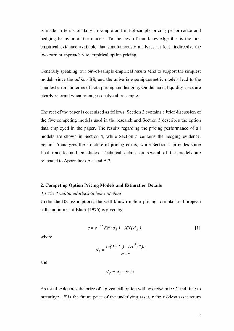
Under the BS assumptions, the well known option pricing formula for European

calls on futures of Black (1976) is given by

)d(XN)d(FNec 21r −= − τ [1]

where

τστσ )2()XFln(d

21

+=

and

τσ−= 12 dd

As usual, c denotes the price of a given call option with exercise price X and time to

maturityτ . F is the future price of the underlying asset, r the riskless asset return

6

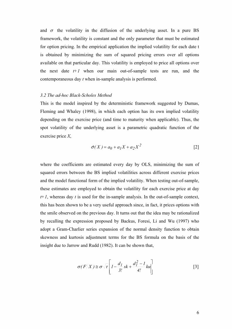
and σ the volatility in the diffusion of the underlying asset. In a pure BS

framework, the volatility is constant and the only parameter that must be estimated

for option pricing. In the empirical application the implied volatility for each date t

is obtained by minimizing the sum of squared pricing errors over all options

available on that particular day. This volatility is employed to price all options over

the next date t+1 when our main out-of-sample tests are run, and the

contemporaneous day t when in-sample analysis is performed.

3.2 The ad-hoc Black-Scholes Method

This is the model inspired by the deterministic framework suggested by Dumas,

Fleming and Whaley (1998), in which each option has its own implied volatility

depending on the exercise price (and time to maturity when applicable). Thus, the

spot volatility of the underlying asset is a parametric quadratic function of the

exercise price X,

2210 XaXaa)X(ˆ ++=σ [2]

where the coefficients are estimated every day by OLS, minimizing the sum of

squared errors between the BS implied volatilities across different exercise prices

and the model functional form of the implied volatility. When testing out-of-sample,

these estimates are employed to obtain the volatility for each exercise price at day

t+1, whereas day t is used for the in-sample analysis. In the out-of-sample context,

this has been shown to be a very useful approach since, in fact, it prices options with

the smile observed on the previous day. It turns out that the idea may be rationalized

by recalling the expression proposed by Backus, Foresi, Li and Wu (1997) who

adopt a Gram-Charlier series expansion of the normal density function to obtain

skewness and kurtosis adjustment terms for the BS formula on the basis of the

insight due to Jarrow and Rudd (1982). It can be shown that,

−+−≅ ku

!41dsk

!3d1)XF(

211τσσ [3]

7

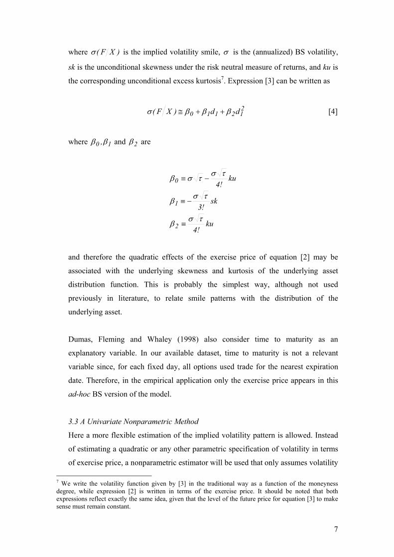
where )XF(σ is the implied volatility smile, σ is the (annualized) BS volatility,

sk is the unconditional skewness under the risk neutral measure of returns, and ku is

the corresponding unconditional excess kurtosis7. Expression [3] can be written as

212110 dd)XF( βββσ ++≅ [4]

where 10 ,ββ and 2β are

ku!4

sk!3

ku!4

2

1

0

τσβ

τσβ

τστσβ

≡

−≡

−≡

and therefore the quadratic effects of the exercise price of equation [2] may be

associated with the underlying skewness and kurtosis of the underlying asset

distribution function. This is probably the simplest way, although not used

previously in literature, to relate smile patterns with the distribution of the

underlying asset.

Dumas, Fleming and Whaley (1998) also consider time to maturity as an

explanatory variable. In our available dataset, time to maturity is not a relevant

variable since, for each fixed day, all options used trade for the nearest expiration

date. Therefore, in the empirical application only the exercise price appears in this

ad-hoc BS version of the model.

3.3 A Univariate Nonparametric Method

Here a more flexible estimation of the implied volatility pattern is allowed. Instead

of estimating a quadratic or any other parametric specification of volatility in terms

of exercise price, a nonparametric estimator will be used that only assumes volatility 7 We write the volatility function given by [3] in the traditional way as a function of the moneyness degree, while expression [2] is written in terms of the exercise price. It should be noted that both expressions reflect exactly the same idea, given that the level of the future price for equation [3] to make sense must remain constant.

8

to be a smooth function of exercise price. A similar approach is considered by Aït-

Sahalia and Lo (1998). However, we propose a different nonparametric technique

that, as we argue below, is especially appropriate for option pricing data. In

particular, the Symmetrized Nearest Neighbor (SNN) estimator is selected, since it

presents better properties when the explanatory variable does not present a uniform

design. In our case, the explanatory variable is the exercise price, which is far from

being uniform, and the SNN estimation procedure rather than the traditional kernel

estimator is the natural choice. This point has not been recognized by previous

empirical applications of nonparametric methods to option data.

Let us briefly describe both kernel and SNN nonparametric regressions. Given the

options available on a particular day t, the dataset tΩ will contain the information

tiii X, ∈σ where iσ denotes the implied volatility for the ith option, and iX its

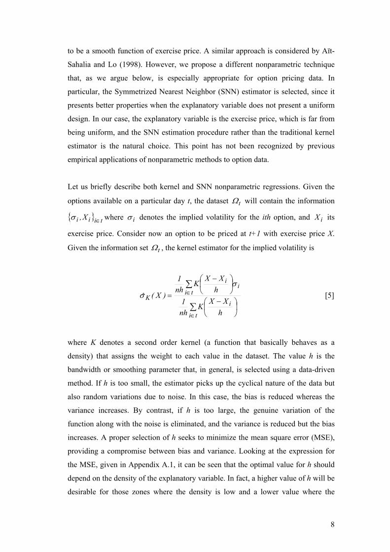
exercise price. Consider now an option to be priced at t+1 with exercise price X.

Given the information set tΩ , the kernel estimator for the implied volatility is

∑

∑

∈

∈

−

−

=

ti

i

tii

i

K

hXX

Knh1

hXX

Knh1

)X(ˆσ

σ [5]

where K denotes a second order kernel (a function that basically behaves as a

density) that assigns the weight to each value in the dataset. The value h is the

bandwidth or smoothing parameter that, in general, is selected using a data-driven

method. If h is too small, the estimator picks up the cyclical nature of the data but

also random variations due to noise. In this case, the bias is reduced whereas the

variance increases. By contrast, if h is too large, the genuine variation of the

function along with the noise is eliminated, and the variance is reduced but the bias

increases. A proper selection of h seeks to minimize the mean square error (MSE),

providing a compromise between bias and variance. Looking at the expression for

the MSE, given in Appendix A.1, it can be seen that the optimal value for h should

depend on the density of the explanatory variable. In fact, a higher value of h will be

desirable for those zones where the density is low and a lower value where the

9

density is high. To deal with this fact a kernel with a variable smoothing parameter

might be a solution, although it turns out to be difficult to implement and its

performance in practice is not satisfactory8.

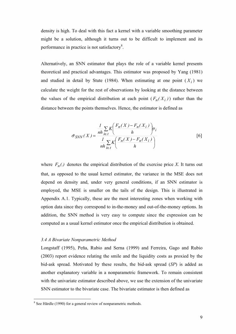
Alternatively, an SNN estimator that plays the role of a variable kernel presents

theoretical and practical advantages. This estimator was proposed by Yang (1981)

and studied in detail by Stute (1984). When estimating at one point ( iX ) we

calculate the weight for the rest of observations by looking at the distance between

the values of the empirical distribution at each point ( )X(F in ) rather than the

distance between the points themselves. Hence, the estimator is defined as

∑

∑

∈

∈

−

−

=

ti

inn

tii

inn

SNN

h)X(F)X(F

Knh1

h)X(F)X(F

Knh1

)X(ˆσ

σ [6]

where (.)Fn denotes the empirical distribution of the exercise price X. It turns out

that, as opposed to the usual kernel estimator, the variance in the MSE does not

depend on density and, under very general conditions, if an SNN estimator is

employed, the MSE is smaller on the tails of the design. This is illustrated in

Appendix A.1. Typically, these are the most interesting zones when working with

option data since they correspond to in-the-money and out-of-the-money options. In

addition, the SNN method is very easy to compute since the expression can be

computed as a usual kernel estimator once the empirical distribution is obtained.

3.4 A Bivariate Nonparametric Method

Longstaff (1995), Peña, Rubio and Serna (1999) and Ferreira, Gago and Rubio

(2003) report evidence relating the smile and the liquidity costs as proxied by the

bid-ask spread. Motivated by these results, the bid-ask spread (SP) is added as

another explanatory variable in a nonparametric framework. To remain consistent

with the univariate estimator described above, we use the extension of the univariate

SNN estimator to the bivariate case. The bivariate estimator is then defined as

8 See Härdle (1990) for a general review of nonparametric methods.

10

∑

∑

∈

∈

−

−

−

−

=

ti SP

inn

X

inn

SPX

tii

SP

inn

X

inn

SPXSNN

h)SP(F)SP(F

Kh

)X(F)X(FK

hnh1

h)SP(F)SP(F

Kh

)X(F)X(FK

hnh1

)X(ˆσ

σ [7]

where the information set for each day will also include the bid-ask spread of the

options; that is, tiiiit SP,X, ∈= σΩ . The statistical properties from the univariate

estimator do not translate straightforwardly to the multivariate setting. However, the

main result remains true and, under very general conditions, the performance of the

bivariate SNN estimator is better in the tails of the marginal distributions for the

covariates. Some theoretical results are also provided in Appendix A.1 and a more

detailed study can be found in Ferreira and Gago (2002), where a simulation study is

carried out that supports the theoretical results.

In the implementation of our two nonparametric regressions discussed above, a

Gaussian kernel has been selected, although any other second order kernel would

lead to similar results. Several methods for selecting smoothing parameters can be

considered for the univariate case. As a general classification, we have the so called

plug-in approach, leave-one-out methods and methods based on penalizing the sum

of residuals9. The resulting estimator depends crucially on the parameter choice and

therefore, the selection procedures matters. Since different methods may end up

with different estimations, we have computed the estimators using three different

alternatives. The first is the univariate plug-in method of Gasser, Kneip and Köhler

(1991). The second and third are the natural extensions of the Generalized Cross

Validation (GCV) and Rice criteria to the bivariate case. As it turns out, the results

are very similar for all of them and the main conclusions remain the same

independently of the method used in practice. In the empirical results below we

report only the estimations obtained with the Rice method.

Let us describe the steps involved in the empirical application. For each option

traded on day t, the procedure to estimate the implied volatility goes as follows: (i)

9 See Härdle (1990).

11

the smoothing parameters are computed each month with all data available and

remain fixed until the next month; (ii) the bid-ask spread is estimated as the average

of the relative bid-ask of all options of the same class, with the same time to

maturity and exercise price, traded on t and t+1 until just before the corresponding

option is observed; (iii) given the smoothing parameters and the bid-ask spread

estimate, the implied volatility is estimated using the information set tΩ and

applying the formula for )X(ˆ SNNσ in the univariate case and )SP,X(ˆ SNNσ in the

bivariate case; (iv) the estimated volatility is then plugged in the BS formula to price

all options at t+110. This implies that under the SNN nonparametric volatity

functions both with and without liquidity costs we obtain semiparametric theoretical

option prices11.

Some remarks are in order. The univariate nonparametric method is similar in spirit

to the ad-hoc volatility estimation procedure. The difference relies on the flexibility

of the implied volatility function allowed by the SNN procedure. The price for

flexibility is a slower rate of convergence to the true function. This means that if the

function is indeed quadratic, as considered in the ad-hoc BS model, this method

should better capture this pattern. However, if the function presents a different

pattern, the ad-hoc BS method leads to wrong estimates while the nonparametric

estimator is still consistent, due to its independence of the particular specification

for the volatility function.

3.5 The HN GARCH Method

All the above methods are useful for practical purposes although they do not

explicitly explain the reasons for the underlying path that determines the volatility

pattern; they just take this pattern as given and try to estimate it by the most

reasonable procedure. They are based merely on the simple idea that an adaptive

estimation of the implied volatility should improve the BS pricing formula.

As a final competing model, we consider the HN (2000) GARCH(1,1) option

pricing formula as particularly appealing because it permits us to capture the path

10 In the in-sample analysis only information up to date t is employed. 11 This is like Aït-Sahalia and Lo (1998). See their discussion on the dimensionality problem.

12

dependence in volatility as well as the negative correlation of volatility with index

returns. Moreover, a closed-form pricing formula is obtained. From a practical point

of view, the HN model presents an advantage with respect to Heston´s (1993)

continuous-time approach. The model is discrete and the parameters can be

estimated using maximum likelihood. Moreover, the asymmetric GARCH(1,1)

version has a continuous limit that is identified as Heston´s model with perfect

correlation between the underlying asset and the volatility. This implies that neither

the volatility risk premium nor the jump-risk premium exist in this framework. Also,

for the purpose of comparing pricing methods, the HN model can be considered as a

model with predictable volatility, since volatility can be estimated from the past

information of the underlying return path. Therefore, a good empirical performance

would provide evidence in favour of deterministic volatility models, frequently

updated, rather than models considering new risk factors. Once again, the idea is to

check whether this simple discrete-time model is rich enough to incorporate the

peculiarities of option prices.

The HN model considers that the log-spot asset price, lnS(t), is characterized by the

following GARCH(1,1) process:

)t(z)t(h)t(h r)t(Sln)t(Sln +++−= λ∆ [8]

( )2)t(h)t(z)t(h)t(h ∆γ∆α∆βω −−−+−+= [9]

where h(t) is the conditional variance of the log return between ∆−t and t and is

predictable from the information set at time ∆−t ; λ is the risk premium embedded

in returns; z(t) is a standard normal disturbance, and the parameter γ controls the

skewness of the distribution.

The model allows for the prediction of )t(h ∆+ at time t from the spot price as

( ))t(h

)t(h )t(h r)t(Sln)t(Sln)t(h)t(h2γλ∆αβω∆ −−−−−

++=+ [10]

13

where α determines the kurtosis of the distribution, and because of the asymmetric

parameter, γ , a large negative shock, )t(z , raises the variance more than a large

positive shock. This model enables us to capture the observed negative correlation

between returns and variance. In particular,

[ ] )t(h 2)t(Sln),t(hcovt γα∆∆ −=+− [11]

where, given a positive α , positive values for γ result in negative correlation

between returns and variance.

To obtain the pricing formula, the process is written in terms of the risk-neutral

measure and it can be shown that the value of a call option is given by

[ ]21r XPP)t(Fec −= − τ [12]

where, as in the BS formula, 2P is the risk neutral probability of the asset being

greater than X at maturity and 1P corresponds to the delta of the call value. Of

course, the computation of 1P and 2P in this case requires estimates of the risk-

neutral parameters in the GARCH model. A more detailed description of the pricing

procedure is given in Appendix A.2.

For empirical analysis the model is estimated daily and for the out-of-sample tests

the parameters obtained with data up to day t are used to price the options traded at

t+1. As with other models, for the in-sample case, only information available up to

date t is employed to price options traded at t. Thus, the parameters are estimated

daily and recursively with two years and one month of past data, or 522 daily

observations of the index return12. The only parameter that needs to be changed in

12 We have both closing price daily returns for the IBEX-35 from January 1994 to November 1998, and 15-minute returns from 1996 to 1998. The daily returns are used in the estimation of the NH GARCH model, and it is therefore the basic data to estimate the conditional daily volatility during our sample period. The rationality of using two years of daily past data to estimate parameters comes from the experience of León and Mora (1999) when estimating several models of the GARCH family with Spanish data. The additional month is due to the maximum length period of the nearest expiration contracts of the options in our dataset.

14

the option pricing formula is the skewness parameter γ which, under the risk

neutral process, turns out to be equal to 21* ++= λγγ . Proceeding in this way,

the model does not really need data from option prices. However, in order to

incorporate simultaneously information from the option and common stock markets,

the risk neutral skewness parameter *γ is implicitly computed from the cross-

section of option prices. The implicit estimator is defined as the minimizer of the

pricing errors in the options traded at time t; that is,

( )∑ −=

∈ti

2ii,HN

*t c)(cminarg γγ

γ, where ic is the price observed in the market, and

)(c i,HN γ denotes the price resulting from the HN formula, where the rest of

parameters are those estimated from the underlying asset return time series. Given

all parameter estimates available at data t, the HN formula is applied to obtain the

out-of-sample price of each option at t+1, and the in-sample price at day t.

As discussed above, and unlike the continuous-time stochastic volatility version of

the model, all the parameters may be estimated directly from the daily closing

returns of the IBEX-35 index using the well known maximum likelihood estimation

proposed by Bollerslev (1986). To illustrate the behavior of the GARCH model,

Table 1 shows the maximum likelihood estimates of the model on the daily IBEX-

35 data from January 1996 to November 1998. The skewness parameter,γ , is

positive and significantly different from zero, indicating that shocks to returns and

volatility covary negatively. The parameter that measures the degree of mean

reversion, given by 2αγβ + and equal to 0.944, is higher than the estimate reported

by HN for the US market. The volatility of volatility, α , is small but also

statistically significant, and the annualized long-run mean of volatility, as given by

)1()(252 2αγβαω −−+ (assuming 252 trading days), is 21.7%. Although not

reported, the restricted version of the model with 0=γ is rejected using both the

log-likelihood ratio test and the SIC statistic.

[Table 1 around here]

15

3. Option Data Description

The Spanish IBEX-35 index is a value-weighted index comprising the 35 most

liquid Spanish stocks traded in the continuous auction market system. The official

derivative market for risky assets, which is known as MEFF, trades a futures

contract on the IBEX-35, the corresponding option on the IBEX-35 futures contracts

for calls and puts, and individual option contracts for blue-chip stocks.

The Spanish option contract on the IBEX-35 futures is a cash settled European

option with trading over the three nearest consecutive months and the other three

months of the March-June-September-December cycle. The expiration day is the

third Friday of the contract month. Prices are quoted in full points, with a minimum

price change of one index point. The exercise prices are given by 50 index point

intervals.

Our database comprises of all call and put options on the IBEX-35 index futures

traded daily on MEFF during the period January 1996 through November 199813.

Liquidity is concentrated on the nearest expiration contract. In fact, during the

sample period almost 90% of trades occurred in this type of contract. Given the

concentration in liquidity, our daily set of observations includes only calls and puts

with the nearest expiration date.

For each option traded we have the transaction price, the relative bid-ask spread, the

exercise price, the expiration date, the simultaneous future price as measured by its

bid-ask spread average, and the annualized repo T-bill rates with approximately the

same maturity as the option.

We restrict our attention to options transacted from 11:00 to 16:45. Every trade

recorded during this window is used in the estimation. Note that care has also been

taken to eliminate the artificial trading potential problems associated with market

makers margin requirements, and also with the well known intraday seasonalities on

13 It may seem appropriate to extend the sample period. However, the structural organization of the Spanish market and its liquidity has changed importantly over time. We argue that our sample period may be characterized as a very homogeneous time period and, in this sense, it is quite useful for our objectives.

16

the underlying index behavior. Finally, we eliminate all call and put prices that

violate the well known arbitrage bounds given by14,

( )

( ) τ

τ

r

r

eFXp

eXFc

−

−

−≥

−≥

These exclusionary criteria yield a final daily sample of 30542 observations (18656

calls and 11886 puts). Table 2 describes the sample properties of the call and put

option prices employed in this work. Average prices, average relative bid-ask

spread, average number of contracts per day and the number of options are reported

for each moneyness category. Moneyness is defined as the ratio of the exercise price

to futures price. A call (put) option is said to be deep out-of-the-money (deep in-the-

money) if the ratio X/F is greater than 1.03; out-of-the-money (in-the-money) if 1.03

≥ X/F > 1.01; at-the-money when 1.01 ≥ X/F > 0.99; in-the-money (out-of-the-

money) when 0.99 ≥ X/F > 0.97; and deep-in-the-money (deep out-of-the-money) if

0.97 > X/F. The average option price ranges from 60.7 pesetas for deep out-of-the-

money calls (deep in-the-money puts) to 110.2 pesetas for at-the-money options. As

expected, the extreme options (in terms of moneyness) have the highest bid-ask

spreads. In other words, deep out-of-the-money (in-the-money) options have the

highest liquidity cost, while at-the-money options have the lowest.

[Table 2 around here]

4. Pricing Performance

4.1 Testing the Statistical Performance of Competing Models

This section reports both in-sample and out-of-sample daily pricing performance of

the five competing models analyzed by our paper. The statistical significance of

performance for in-sample and out-of-sample pricing errors is assessed first by

analyzing the proportions of theoretical prices lying outside their corresponding bid-

ask boundaries. Then we test whether or not the differences between proportions of

14 Approximately 1.1% of all options in the dataset violated these arbitrage bounds.

17

any two competing models are statistically different from zero, taking into account

that any two competing models are not independent.

Specifically, we take any pair of two models. Let 1p be the proportion of calls

(puts) whose theoretical price lies outside the bid-ask spread when we price with

model 1, and let 2p be the corresponding proportion when we price with model 2.

Also, let 1Z be 1 if the theoretical price (for model 1) is outside the spread and 0

otherwise. Finally, 2Z is 1 if the theoretical price (for model 2) is outside the spread

and 0 otherwise. Then, 21 ZZ − equals -1 with probability 1π , 0 with probability

2π , and 1 with probability 211 ππ −− . Under the null hypothesis of equal

proportions,

1

2112

21

2)ZZvar(

210)ZZ(E

π

ππ

=−

−=⇒=−

Note that,

1n

1i

1i pZ

n1

=∑=

2n

1i

2i pZ

n1

=∑=

Consider the statistic defined as,

( ) ( )[ ]2n

1n

21

11 ZZ...ZZ

n1Z −++−= [13]

by the Central Limit Theorem,

→

n2,0 NZ 1π

where 1π can be estimated as

18

2nones minus of no. ones of no.

ˆ 1+

=π

Since the differences in proportions coincide with the Z-statistic, then the final

statistic employed to compare the models is given by

→−=nˆ2

,0NppZ 121 π [14]

We also compare the performance of all models by analyzing prices inferred from

each theoretical model against the observed market prices. In particular, we compute

for each model the absolute pricing error as given by the square root of the squared

differences between the theoretical price and the market price of each option i:

( )∑ −==

n

1i

2mket,ielmod,i PPn1APE [15]

where n is the number of options, and elmod,iP and mket,iP are the theoretical price

for either a call or a put for each of the five models, and the observed market price

respectively.

To test statistically whether the average absolute pricing errors of two competing

models are significantly different from zero, we perform a GMM overidentifying

restriction test, with the Newey-West weighting covariance matrix. We consider the

following set of moment conditions for any two competing models

=

−∑

−∑

=

−=

−

00

mAPEn

mAPEn

n

1i

2i

1

n

1i

1i

1

[16]

where 2,1iAPE is the absolute pricing error for option i and either model 1 or 2, and

m is the common mean pricing error under the null hypothesis that both models

19

have the same pricing error. The test statistic is distributed as a 2χ with one degree

of freedom.

4.2 In-Sample Pricing Performance

The statistical in-sample performance of all models using the proportion that the

theoretical price is outside the bid-ask spread is contained in Table 3 for both calls

and puts. The figures in each panel are the proportions of theoretical prices lying

outside the spread for options within a moneyness category15, and below the

identifying number of the competing model that has a significantly lower proportion

than the model being analyzed according to our Z-statistic in equation [14]. As an

example, and in order to facilitate the reading of the following tables, note that the

semiparametric model with liquidity costs has 16.4% of all call prices outside the

observed bid-ask spread. Moreover, analyzing the statistical significance of that

proportion relative to the proportion associated with any other model by Z-statistic,

we conclude that this proportion is statistically different (lower) than the proportions

given by BS (model 1), the semiparametric model with the nonparametric volatility

function depending only on the exercise price (model 2), the ad-hoc BS (model 4),

and HN (model 5). Therefore, for call options the flexible semiparametric model

with liquidity costs presents a statistically better performance than the rest of

models. Interestingly, however, ATM calls are better priced in the sense defined

above by the the ad-hoc BS. As expected, under the net buying pressure hypothesis

and for calls, liquidity costs are more relevant for options with extreme moneyness

degrees. At the same time, theoretical put prices always present statistically lower

proportions outside the bid-ask boundary when liquidity costs are included. The

flexibility of the nonparametric estimation of the volatility function together with

liquidity costs seems to be a key consideration when pricing options in-sample. It is

important to note, however, that the key in understanding the results lies in the

impact of liquidity costs rather than in the flexible functional form of the volatility

function. The ad-hoc BS has lower proportions of theoretical prices outside the

spread when compared to the semiparametric model with the exercise price as the

only explanatory variable. Indeed, the quadratic parametric representation of the

15 In Tables 3 to 7, deep in-the-money (out-of-the-money) calls (puts), and deep out-of-the-money (in-the-money) calls (puts), as reported in Table 1, are now included in the corresponding out-of-the-money and in-the-money categories.

20

volatility function seems to be, on average, a good representation of the volatility

smile.

[Table 3 around here]

When performance is analyzed in terms of pricing differences by the APE statistic

given by equation [15] and the 2χ GMM test in [16], we find very similar results.

The results are reported in Table 4. Again, liquidity costs seem to be a key

consideration when pricing options in-sample. Note that even ATM calls have less

pricing differences. Given that these options have lower proportions outside the

spread when pricing by ad-hoc BS, we may conclude that options which belong to

the 16.9% outside the boundaries, as reported in Table 3, must have quite large

pricing differences to justify the worse performance found under the APE statistic in

Table 4.

[Table 4 around here]

Finally, both the traditional BS model and the HN GARCH(1,1) present a very poor

performance both in terms of proportions outside the bid-ask spread and in terms of

pricing differences. We will come back to these results when analyzing out-of-

sample performance.

4.3 Out-of-Sample Pricing Performance

Of course, from the practitioner’s point of view, it is more relevant to know how

option pricing models value derivatives out-of-sample. This has always been the

important perspective in option modeling. The results using proportions off the

spread are contained in Table 5. As before, they are the frequencies of theoretical

prices lying outside the bid-ask spread, and below the identifying number of the

competing model that has a significantly lower proportion than the model being

analyzed according to our Z-statistic. In this case, and contrary to the in-sample

evidence, the ad-hoc BS dominates all models with 41.0% (39.6%) of all call (put)

prices outside the observed bid-ask spread. Moreover, the proportions observed in

the ad-hoc BS case are statistically lower for all moneyness categories except for in-

21

the-money options. Therefore, the ad-hoc BS presents a statistically superior out-of-

sample performance than the rest of option pricing models considered in the paper16.

[Table 5 around here]

Surprisingly, the out-of-sample results show that the univariate nonparametric

pricing method obtains significantly lower proportions outside the spread than the

model with liquidity costs. First, the fact that a parametric model outperforms the

more flexible approach indicates that again, on average, the symmetric smile rather

than the downward sloping smirk captures the behavior of the distribution of the

underlying asset during this sample period. Note that this ad-hoc parametric model

is consistent with pricing by market makers in actual trading. Secondly, the impact

of moving from in-sample to out-of-sample is quite dramatic. The proportions

outside the spread increase by 100% for the best models, while the frequencies

under BS and HN go up by approximately 14%. Of course, these models present

very high proportions outside the spread for both the in-sample and out-of-sample

cases. It seems therefore that daily market conditions change considerably either

because of variations of moments in the underlying distribution of returns or

because demand conditions vary sufficiently to move prices quite a lot given the

limited supply of contracts provided by market makers. It is probably a combination

of the two factors that plays the key role in explaining out-of-sample performance.

Both rapidly changing market conditions which affect the distribution of returns of

the underlying asset and a limited supply of options having a strong impact on

hedging (and trading) costs lead towards instability of parameters in option pricing

models. Thus, our traditional theoretical framework fails in the out-of-sample

context. Along this line of reasoning, it should be pointed out that recent papers

using Spanish data and variants of an approximation of the risk-neutral density of

terminal underlying prices by the lognormal Gram-Charlier series expansion also

obtain poor out-of-sample performance. Serna (2004) employs this method to

implicitly estimate the risk-neutral skewness and kurtosis of the underlying asset. 16 Using quarterly data, as in Ferreira, Gago and Rubio (2003), the results employing the exercise price or the moneyness degree, as measured by X/F, in the estimation of the volatility function are the same. Note that when using moneyness the issue is to decide the appropriate underlying price. In principle, it should be the same for different exercise prices. In the application with quarterly data, the average of the underlying price during each sample period is taken as a proxy for the denominator. However, to employ this ratio with daily data is more problematic and it is discarded from the estimation.

22

Although a more consistent performance than BS is reported, pricing errors remain

quite substantial. Prado (2004) argues that under this expansion one may obtain a

negative risk-neutral density for some values of skewness and excess kurtosis. He

incorporates the adjustment suggested by Jondeau and Rockinger (2001) to

guarantee the positivity of the Gram-Charlier risk-neutral density and, as before,

out-of-sample performance is quite disappointing. Similar results are obtained by

León, Mencía and Sentana (2004) using semi-nonparametric densities of Gallant

and Nychka (1987) which are always positive and more general than the truncated

Gram-Charlier expansions. Hence, relaxing the assumption of lognormality does not

seem to be sufficient to adequately price options out-of-sample.

It is also the case that liquidity costs, as proxied by the past bid-ask spreads, do not

improve option pricing performance. This is consistent with the evidence reported

by Peña, Rubio and Serna (2001) using a parametric approach within an out-of-

sample context, and it suggests that past spreads are not useful in characterizing

current market conditions. Again, it is difficult to rationalize this evidence without

recurring to limited supply arguments in the option market.

To conclude, models based on smooth functions of volatility do not capture the

underlying behavior of the underlying asset or of its volatility, and they seem to be

useless in explaining the idiosyncratic characteristics of the internal organization of

option markets.

The extremely poor performance of the HN model is also striking but, at the same

time, very informative on what is missing from GARCH option pricing. Figure 1

contains the daily implied BS volatility and the daily conditional volatility estimated

by expression [10]. During most of the sample period, the volatility estimated by the

HN GARCH model undervalues the implied volatility from the cross-section of

available options. This is a very important point. The implicit estimation of the

skewness parameter is not sufficient to introduce the information contained in the

cross-section of option prices17. It should be noted that the HN model is the only one

17 Despite the fact that Christoffersen and Jacobs (2003) argue that GARCH models with volatility clustering and standard asymmetric effects like the one suggested by HN perform well compared to less parsimonious alternative models.

23

in which the estimate of volatility does not employ option data. In our case, this

makes its pricing performance to be very poor relative to all other models, including

the traditional BS method18. Given the lack of integration between the underlying

and option markets, employing parameters estimated directly from the underlying

return process does not seem to help out-of-sample pricing19.

[Figure 1 around here]

Independently of the above arguments, the GARCH methodology is not clearly

appropriate for inferring future volatility in the option pricing context. It should be

recalled that we are dealing with short-term option data. In fact, HN report that their

model does not improve on the ad-hoc BS model when they price the shortest to

maturity options in their US database. Their GARCH modeling of variance is not

able to reproduce the rapidly increasing behavior of conditional volatility needed to

price short-term options, despite the fact that the model adapts to changes in

volatility associated with changes in market levels. Note that jumps in returns can

generate large movements, but the impact of a jump is transitory and consequently

does not affect future prices. On the other hand, conditional volatility is persistent

but it may only increase via small gradual normally distributed steps. In order to

allow conditional volatility of returns to increase quickly, it becomes necessary to

permit jumps in volatility on the underlying data generating process of equity

returns. This is the point raised by Eraker, Johannes and Polson (2003) and Eraker

(2004) who model jumps in volatility with constant arrival intensity and constant

amplitude. However, as mentioned in our introductory comments, this approach is

not flexible enough to explain the cross-section of option prices. Moreover, GARCH

option modeling with jumps in volatility has not yet been developed, even under the

simplest specification.

Finally, it has been recently argued by Ghysels, Santa-Clara and Valkanov (2004)

that the so called mixed data sampling regression (MIDAS) framework is more

appropriate than GARCH modeling when predicting volatility. Its success is based

on the additional power of using more data, estimating less parameters and,

18 Similar results are found when the sample is divided into three independent years. 19 Not even in-sample performance.

24

especially, because of the more flexible (and optimum) weighting scheme employed

when incorporating past volatility. In particular, the asymmetry in the response of

the conditional volatility to positive and negative returns is more complex than

previously recognized by the GARCH family. According to their evidence, negative

shocks have a higher immediate effect but are ultimately dominated by positive

innovations. Simultaneously, there is a strong asymmetry in the persistence of

positive and negative shocks, with positive shocks being responsible for the

persistence of the conditional volatility for horizons beyond two or three weeks of

trading20. By construction, these effects are not captured by any GARCH model.

This recent evidence casts doubts on the validity of GARCH option modeling and it

may also be responsible in part for the extremely poor performance of the HN

model.

The out-of-sample performance of pricing errors using the APE statistic tends to

give similar results. They are reported in Table 6. The ad-hoc BS pricing model and

the flexible univariate semiparametric option model are the best performing models.

As before, there is a slight advantage for the ad-hoc BS, but the differences between

the two models are less pronounced than when using proportions lying outside the

bid-ask spread.

[Table 6 around here]

5. Hedging Performance

The analysis of hedging performance follows Bakshi, Cao and Chen (1997), in

which a single instrument is employed. The objective is to hedge a short position for

a call option with τ periods to expiration and exercise price X. Let F∆ be the

number of shares in the underlying asset to be purchased and let FcB F∆−=0 be

the residual position, so that the value of a replicating portfolio at t is )t(FB F∆+0 .

Solving the standard minimum variance hedging problem, the option delta, F∆ , has

the expression

20 These results have been confirmed by León, Nave and Rubio (2004) using European equity indices including the IBEX-35 index.

25

)d(NePeF

),,r,X,F(c rrF 11

ττστ∆ −− ==∂

∂= [17]

where we recall that the term 1d is given in equation [1].

Therefore, the different methods proposed in Section 2 for estimating volatility lead

to different deltas. If the HN formula is used, the delta of the option has also the

form 1Pe rF

τ∆ −= , where 1P is different from the normal distribution, and it depends

on the parameters in the GARCH model, as described in Appendix A.2.

For all models, we assume that portfolio rebalancing takes place at intervals of

length t δ (either a day or a week)21. Once the delta is estimated for each option in

the sample, we obtain the resulting cash position as FˆcB F∆−=0 which we invest

in the equivalent maturity risk free bond. At time t t δ+ we calculate the hedging

error for each model as

)t ,t t(ceB)t t(Fˆ)t t(H t rF δτδδ∆δ δ −+−++=+ 0 [18]

For computation of the hedging errors, we employ the first option in each class

(same time to maturity and exercise price) that appears in the 45-minute window

between 16:00 and16:45 for both t and t t δ+ 22.

To analyze the differences in hedging behavior between our competing models, we

calculate the average absolute hedging error for each model as

∑=

=n

iiH

nH

1

1 [19]

where n is the number of options over the complete sample period.

21 Although the hedging errors become larger when one week is employed, qualitative conclusions are the same, and the results reported below only contain portfolio rebalancing taking place at intervals of one day. 22 As an alternative, the hedging performance for the last option traded in each class during each day has been analyzed and the results remain the same.

26

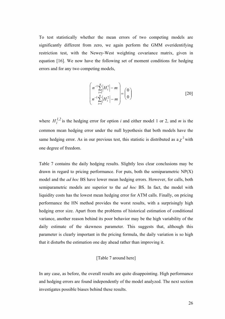
To test statistically whether the mean errors of two competing models are

significantly different from zero, we again perform the GMM overidentifying

restriction test, with the Newey-West weighting covariance matrix, given in

equation [16]. We now have the following set of moment conditions for hedging

errors and for any two competing models,

=

−

−

∑

∑

=

−

=

−

00

1

21

1

11

n

ii

n

ii

mHn

mHn [20]

where 2,1iH is the hedging error for option i and either model 1 or 2, and m is the

common mean hedging error under the null hypothesis that both models have the

same hedging error. As in our previous test, this statistic is distributed as a 2χ with

one degree of freedom.

Table 7 contains the daily hedging results. Slightly less clear conclusions may be

drawn in regard to pricing performance. For puts, both the semiparametric NP(X)

model and the ad hoc BS have lower mean hedging errors. However, for calls, both

semiparametric models are superior to the ad hoc BS. In fact, the model with

liquidity costs has the lowest mean hedging error for ATM calls. Finally, on pricing

performance the HN method provides the worst results, with a surprisingly high

hedging error size. Apart from the problems of historical estimation of conditional

variance, another reason behind its poor behavior may be the high variability of the

daily estimate of the skewness parameter. This suggests that, although this

parameter is clearly important in the pricing formula, the daily variation is so high

that it disturbs the estimation one day ahead rather than improving it.

[Table 7 around here]

In any case, as before, the overall results are quite disappointing. High performance

and hedging errors are found independently of the model analyzed. The next section

investigates possible biases behind these results.

27

6. The Structure of Pricing Errors

A further analysis trying to understand the structure of the out-of-sample pricing

errors of these models would seem to be called for. We now use a simple regression

framework to study the relationship between percentage pricing errors and factors

that are either option-specific or market dependent. We first take as given an option

pricing model, and let ite be the ith option’s percentage pricing error on day t

defined as the theoretical price minus the market price, divided by the market price.

Finally, we run the following regression for the whole sample period and for calls

and puts separately:

ititittttitit SPbXlnbKUbSKbbbae εστ +++++++= 654321 [21]

where itτ is the annualized time to maturity of the ith option at day t, tσ is the

annualized daily standard deviation of the IBEX-35 index returns computed from

15-minute intradaily returns, and similarly tSK and tKU are the daily skewness

and the (excess) kurtosis at day t respectively; itX is the exercise price and itSP is

the relative bid-ask spread of the ith option. The results are reported in Table 8,

where the results for calls and puts are reported separately. As can be observed, the

explanatory variables are significantly different from zero in almost all cases. These

results provide evidence against models trying to explain the time-varying behavior

of the volatility function as a smooth function of previously defined variables, be it

in an ad hoc way, in a GARCH parametric framework or in our nonparametric

context. The results are consistent with the need to simultaneously incorporate a

more complex behavior in the process of returns and volatility with (probably)

correlated jumps and the effects of organizational characteristics of the option

market.

[Table 8 around here]

It is interesting to notice the large biases associated with the HN model. The

(negative) magnitude of the 2b coefficient related to the model is very high and

significant. It is the largest coefficient (in absolute value) of all the models, and it

28

reflects that the conditional variance estimated with historical return data

undervalues the variance reflected in option prices, particularly when there is a lot of

variability in the market. This is clearly consistent with Figure 1. As expected, the

second largest coefficient (in absolute value) comes from the BS model, where

constant volatility across options is imposed. Moreover, again for these two models,

the 1b coefficients are also large. Thus, they reflect a large time to maturity bias for

both calls and puts. As reflected in the magnitude of the coefficients, the most

problematic pricing performance of the two models tends to be associated with

options with the longest time to expiration. Hence, the deficiencies discussed for

these models become more pronounced with options that have more days to

maturity. In any case, it should be recognized that, at least for puts, all pricing

models except the univariate semiparametric case have more difficulties in pricing

options as time to expiration becomes longer.

Finally, the coefficient associated with the bid-ask spread is again large in the HN

case. If the underlying asset and the option market are not fully integrated, any

model estimating most relevant parameters only from the stock market will be

unable to capture idiosyncratic characteristics of option prices.

In short, neither model seems to reflect appropriately the underlying distribution

characteristics of the IBEX-35 and/or the idiosyncratic characteristics of the option

market microstructure.

7. Conclusions

In this paper, we employ intraday option data from the Spanish market to test both

the pricing and hedging performance of the five option pricing models. The results

show that, from the out-of-sample point of view, simplicity is an important

characteristic in the option pricing framework used. The ad-hoc BS and the simplest

univariate semiparametric models are the best performing models. In fact, the

overall picture suggests that the ad-hoc BS is slightly superior despite the flexibility

added by the nonparametric estimation of the volatility function. However, the

overall out-of-sample performance of all models is quite poor. On the other hand,

in-sample pricing performance shows that liquidity cost is a key issue in option

29

pricing. If our liquidity costs reflect the net buying pressure from public orders, our

evidence may indicate that there exists a strong daily changing behavior in the

demand for options at different exercise prices with an upward sloping supply curve,

given the quite different performance of the model with liquidity costs when we

move from in-sample to out-of-sample tests.

Simultaneously, the overall poor performance of the models may also suggest that

(probably) correlated jumps in returns and volatility are a key feature to be adopted

for any competitive option pricing model. It seems that the volatility function is not

a smooth function of the underlying variables used in the estimation. Also, and

somewhat surprisingly, the HN specification presents a very poor pricing and

hedging performance. The GARCH framework cannot generate (time-varying)

skewness and kurtosis in the degree needed to price options. In other words,

GARCH volatility does not incorporate the rich information contained in the cross-

section of option prices, in spite of the fact that the asymmetric GARCH parameter

is estimated implicitly from option data. The volatility inferred from the history of

the index returns is not high enough to obtain reasonable option prices.

Our results, together with the evidence currently available from stochastic models

with volatility and jump risk factors, suggest that an integrated approach of both

options and stock markets that also incorporates correlated jumps in volatility may

be a promising area of research. Simultaneously, explicit analysis of financial

intermediation of the underlying risks by option market makers and the effects of

time-varying net buying pressure along with upward sloping supply curves in option

prices is probably more effective. Given our experience with option data, we support

microstructure explanations rather than more elaborate (and difficult to estimate)

models23. In any case, further research is clearly justified with a view to

understanding the seemingly rapidly changing behavior of the underlying equity

asset return distribution and net buying pressure conditions as described by Bollen

and Whaley (2004).

23 It must be recognized that we are dealing with options characterized by very short-term to expiration traded in a rather thin option trading market. The results should be taken under this perspective. For example, Huang and Wu (2004) show that the factors dominating short-term and long-term options are substantially different when pricing options within large markets.

30

Appendix A1. The Procedure in the Nonparametric Estimation

We summarize the main results that have motivated the nonparametric estimation

process employed in this work. Proofs and specific details can be found in Ferreira

and Gago (2002).

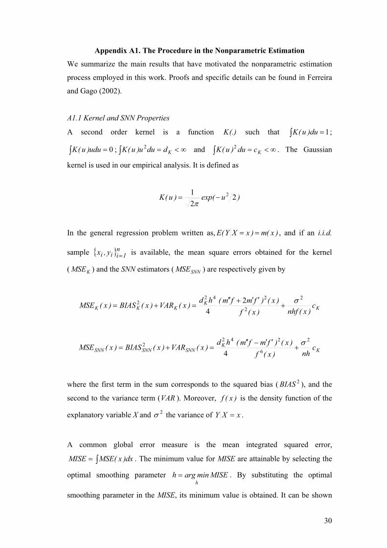
A1.1 Kernel and SNN Properties

A second order kernel is a function (.)K such that ∫ =1du)u(K ;

∫ = 0udu)u(K ; ∫ ∞<= Kdduu)u(K 2 and ∫ ∞<= Kcdu)u(K 2 . The Gaussian

kernel is used in our empirical analysis. It is defined as

)uexp()u(K 221 2−=π

In the general regression problem written as, )x(m)xXY(E == , and if an i.i.d.

sample n1iii y,x = is available, the mean square errors obtained for the kernel

( KMSE ) and the SNN estimators ( SNNMSE ) are respectively given by

KK

KKK c)x(nhf)x(f

)x()fmfm(hd)x(VAR)x(BIAS)x(MSE2

2

2422 2

4σ

+′′+′′

=+=

KK

SNNSNNSNN cnh)x(f

)x()fmfm(hd)x(VAR)x(BIAS)x(MSE2

6

2422

4σ

+′′−′′

=+=

where the first term in the sum corresponds to the squared bias ( 2BIAS ), and the

second to the variance term (VAR ). Moreover, )x(f is the density function of the

explanatory variable X and 2σ the variance of xXY = .

A common global error measure is the mean integrated squared error,

∫= dx)x(MSEMISE . The minimum value for MISE are attainable by selecting the

optimal smoothing parameter MISEminarghh

= . By substituting the optimal

smoothing parameter in the MISE, its minimum value is obtained. It can be shown

31

that, under very general situations, the SNNMISE is smaller than the KMISE in the

tails of the distribution; that is, in those zones where the data density is low.

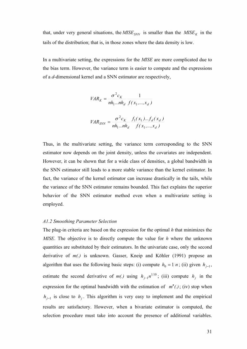
In a multivariate setting, the expressions for the MISE are more complicated due to

the bias term. However, the variance term is easier to compute and the expressions

of a d-dimensional kernel and a SNN estimator are respectively,

)x,...,x(f)x(f)...x(f

nh...nhcVAR

)x,...,x(fnh...nhcVAR

d

dd

d

KSNN

dd

KK

1

11

1

2

11

2 1

σ

σ

=

=

Thus, in the multivariate setting, the variance term corresponding to the SNN

estimator now depends on the joint density, unless the covariates are independent.

However, it can be shown that for a wide class of densities, a global bandwidth in

the SNN estimator still leads to a more stable variance than the kernel estimator. In

fact, the variance of the kernel estimator can increase drastically in the tails, while

the variance of the SNN estimator remains bounded. This fact explains the superior

behavior of the SNN estimator method even when a multivariate setting is

employed.

A1.2 Smoothing Parameter Selection

The plug-in criteria are based on the expression for the optimal h that minimizes the

MISE. The objective is to directly compute the value for h where the unknown

quantities are substituted by their estimators. In the univariate case, only the second

derivative of m(.) is unknown. Gasser, Kneip and Köhler (1991) propose an

algorithm that uses the following basic steps: (i) compute nh 10 = ; (ii) given 1−jh ,

estimate the second derivative of m(.) using 1011nh j− ; (iii) compute jh in the

expression for the optimal bandwidth with the estimation of (.)m ′′ ; (iv) stop when

1−jh is close to jh . This algorithm is very easy to implement and the empirical

results are satisfactory. However, when a bivariate estimator is computed, the

selection procedure must take into account the presence of additional variables.

32

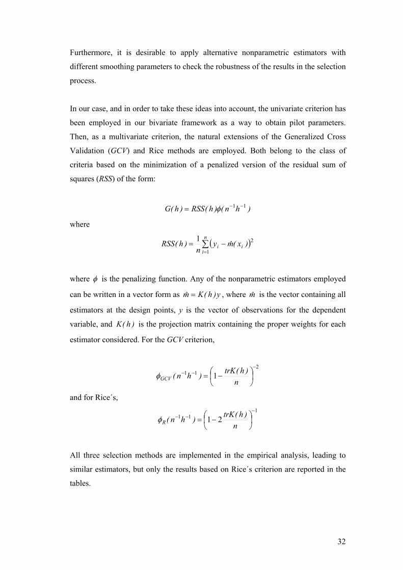
Furthermore, it is desirable to apply alternative nonparametric estimators with

different smoothing parameters to check the robustness of the results in the selection

process.

In our case, and in order to take these ideas into account, the univariate criterion has

been employed in our bivariate framework as a way to obtain pilot parameters.

Then, as a multivariate criterion, the natural extensions of the Generalized Cross

Validation (GCV) and Rice methods are employed. Both belong to the class of

criteria based on the minimization of a penalized version of the residual sum of

squares (RSS) of the form:

)hn()h(RSS)h(G 11 −−= φ

where

( )∑=

−=n

iii )x(my

n)h(RSS

1

21

where φ is the penalizing function. Any of the nonparametric estimators employed

can be written in a vector form as y)h(Km = , where m is the vector containing all

estimators at the design points, y is the vector of observations for the dependent

variable, and )h(K is the projection matrix containing the proper weights for each

estimator considered. For the GCV criterion,

2

11 1−

−−

−=

n)h(trK)hn(GCVφ

and for Rice´s, 1

11 21−

−−

−=

n)h(trK)hn(Rφ

All three selection methods are implemented in the empirical analysis, leading to

similar estimators, but only the results based on Rice´s criterion are reported in the

tables.

33

Appendix A2. The Heston and Nandi (HN) Option Pricing Formula

In the computations, daily returns are considered and therefore ∆ is set equal to 1 in

the HN formula. In this setting, the HN risk-neutral process is given by

( )2111

211

)t(h*)t(*z)t(h)t(h

)t(*z)t(h)t(hr)t(Sln)t(Sln

−−−+−+=

+−+−=

γαβω

where

21

21

++=

++=

λγγ

λ

*

)t(h)t(z)t(*z

The option pricing formula is then given by

[ ]21 XPP)t(Fec rHN −= − τ

where

φφ

φπ

φφ

φπ

φ

φ

d )(*f i

)i(*fXReP

d )(*f i

)i(*fXReP

i

i

∫

∫

∞ −

∞ −

+=

++=

02

01

11

21

111

21

The function )(*f φ corresponds to the conditional generating function of the risk-

neutral process of the asset price. In this case, it takes the log-linear form

[ ] )t(h),T;t(B),T;t(A*t e)t(S)T(SE)(*f 1++== φφφφφ

The terms A(.) and B(.) depend on the set of parameters *),,,( γβαω and the

estimation procedure is performed in a recursive form as

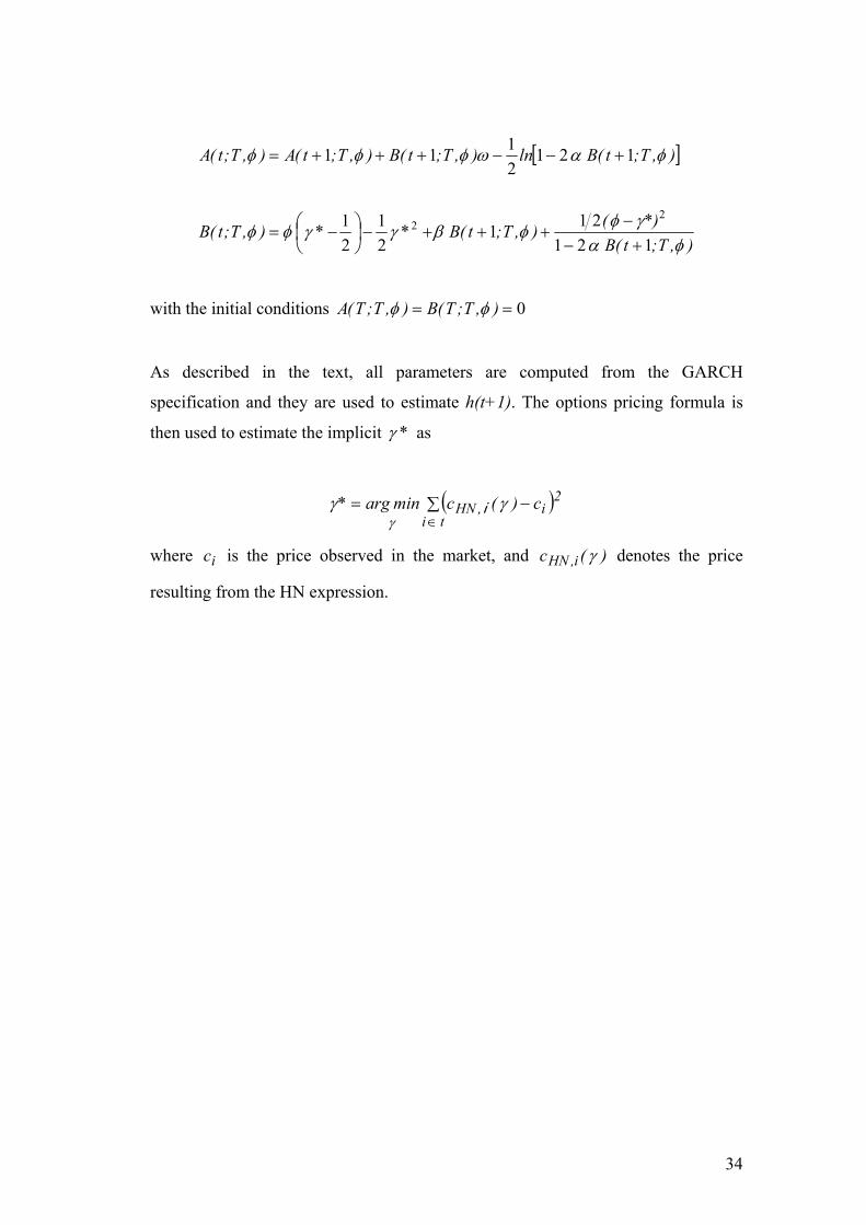
34

[ ]

),T;t(B *)(),T;t(B ** ),T;t(B

),T;t(B ln),T;t(B),T;t(A),T;t(A

φαγφφβγγφφ

φαωφφφ

121211

21

21

1212111

22

+−−

+++−

−=

+−−+++=

with the initial conditions 0== ),T;T(B),T;T(A φφ

As described in the text, all parameters are computed from the GARCH

specification and they are used to estimate h(t+1). The options pricing formula is

then used to estimate the implicit *γ as

( )∑ −=∈ ti

2i,HN c)(cminarg*

i γγ

γ

where ic is the price observed in the market, and )(c i,HN γ denotes the price

resulting from the HN expression.

35

References

Aït-Sahalia, Y., and A. Lo (1998), “Nonparametric estimation of state-price densities

implicit in financial asset prices”, Journal of Finance 53, pp.499-547.

Anderson, T., Benzoni, L., and J. Lund (2002), “An empirical investigation of

continuous-time equity return model”, Journal of Finance 57, pp. 1239-1284.

Backus, D., Foresi, S., Li, K., and L. Wu (1997) “Accounting for biases in Black-

Scholes”, Working Paper, Stern School of Business, New York University.

Bakshi, G., Kapadia, N., and D. Madan (2003), “Stock return characteristics, skew laws,

and the differential pricing of individual equity options”, Review of Financial Studies

16, pp. 101-143.

Bakshi, G., and C. Cao (2003) “Risk-neutral kurtosis, jumps, and option pricing.

Evidence from 100 most actively traded firms on the CBOE”, Working Paper, Smith

School of Business, University of Maryland.

Bakshi, G., Cao, C., and Z. Chen (1997), “Empirical performance of alternative option

pricing models”, Journal of Finance 52, pp. 2003-2049.

Bates, D. (1996), “Jumps and stochastic volatility: exchange rate processes implicit in

Deutsche mark options”, Review of Financial Studies 9, pp. 69-107.

Bates, D. (2000), “Post-`87 crash fears in S&P 500 futures options”, Journal of

Econometrics 94, pp. 181-238.

Bates, D. (2003), “Empirical option pricing: A retrospection”, Journal of Econometrics

116, pp. 387-404.

Black, F. (1976), “The pricing of commodity contracts”, Journal of Financial

Economics 3, pp. 167-179.

36

Black, F. and M. Scholes (1973), “The pricing of options and corporate liabilities”,

Journal of Political Economy 81, pp. 637-659.

Bollen, N., and R. Whaley (2004), “Does net buying pressure affect the shape of

implied volatility functions?”, Journal of Finance 59, pp. 711-753.

Bollerslev, T. (1986), “Generalized autoregressive conditional heteroskedasticity”,

Journal of Econometric 31, pp. 307-327.

Chernov, M. and E. Ghysels (2000), “A study towards a unified approach to the joint

estimation of objective and risk neutral measures for the purpose of option valuation”,

Journal of Financial Economics 56, pp. 407-458.

Christoffersen, P., and K. Jacobs (2003) “Which volatility model for option valuation?”,

Working Paper, Faculty of Management, McGill University.

Duffie, D., Pan, J., and K. Singleton (2000), “Transform analysis and asset pricing for

affine jump-diffusions”, Econometrica 68, pp. 1343-1376.

Dumas, B., J. Fleming and R. Whaley (1998), “Implied volatility functions: empirical

tests”, Journal of Finance, 53, pp. 2059-2106.

Eraker, B. (2004), “Do stock prices and volatility jump? Reconciling evidence from

spot and option prices”, Journal of Finance 59, pp. 1367-1404.

Eraker, B., Johannes, M., and N. Polson (2003), “The impact of jumps in equity index

volatility and returns”, Journal of Finance 58, pp. 1269-1300.

Ferreira, E. and M. Gago (2002) “Kernel vs. SNN estimators in a multivariate context:

An application to finance”, Working Paper, Departamento de Econometría y

Estadística, Universidad del País Vasco.

37

Ferreira, E., Gago, M., and G. Rubio (2003), “A semiparametric estimation of liquidity

effects on option pricing”, Spanish Economic Review Vol 5, 2003, pp. 1-24.

Fiorentini, G., León A. and G. Rubio (2002), “Estimation and empirical performance of

Heston´s stochastic volatility model: the case of a thinly traded market”, Journal of

Empirical Finance, 9, pp. 225-255.

Gallant, A. and D. Nychka (1987), “Seminonparametric maximum likelihood

estimation”, Econometrica 55, pp. 363-390.

Garcia, R., Ghysels, E., and E. Renault (2004) “The econometrics of option pricing”,

Série Scientifique no. 4, CIRANO, Montreal.

Gasser, T., Kneip, A. and W. Köhler (1991), “A flexible and fast method for automatic

smoothing”, Journal of the American Statistical Association, 86, pp. 643-652.

Ghysels, E., Santa-Clara, P., and R. Valkanov (2004) “There is a risk-return tradeoff

after all”, Working Paper, The Anderson School of Management, University of

California at Los Angeles.

Härdle, W. (1990). Applied nonparametric regression, Cambridge University Press,

Cambridge.

Heston, S. (1993), “A closed-form solution for options with stochastic volatility with

applications to bond and currency options”, Review of Financial Studies 6, pp. 327-344.

Heston, S., and S. Nandi (2000), “A closed-form GARCH option valuation model”,

Review of Financial Studies 13, pp. 585-625.

Huang, J, and L. Wu (2004), “Specification analysis of option pricing models based on

time-changed Lévy processes”, Journal of Finance 59, pp. 1405-1440.

Jarrow, R., and A. Rudd (1982), “Approximate option valuation for arbitrary stochastic

processes”, Journal of Financial Economics 10, pp. 347-369.

38

Jondeau, E., and M. Rockinger (2001), “Gram-Charlier Densities”, Journal of

Economics Dynamics and Control 25, pp. 1457-1483.

León, A. and J. Mora (1999), “Modeling conditional heteroskedasticity: Application to

the IBEX-35 stock-return index”, Spanish Economic Review 1, pp. 215-238.

León, A., Mencía, J., and E. Sentana (2004) “Parametric properties of semi-parametric

distributions with applications to option valuation”, Working Paper, CEMFI, Madrid.

León, A., Nave, J., and G. Rubio (2004) “The relationship between risk and expected

return in Europe”, para Fundación BBVA: “Estudios sobre Agregados Económicos

Europeos y Políticas Estructurales”

Longstaff, F.(1995), “Option pricing and the martingale restriction”, Review of

Financial Studies 8, pp. 1091-1124.

Pan, J, (2002), “The jump-risk premia implicit in options: evidence from an integrated

time-series study”, Journal of Financial Economics 63, pp. 3-50.

Peña, I., Rubio, G. and G. Serna (1999), “Why do we smile? On the determinants of the

implied volatility function”, Journal of Banking and Finance 23, pp. 1151-1179.

Peña, I., Rubio, G. and G. Serna (2001), “Smiles, bid-ask spreads and option pricing”,

European Financial Management Journal 7, pp. 351-374.

Prado, J.M. (2004) “IBEX-35 option pricing under alterative models”, Working Paper,

CEMFI, Madrid.

Santa-Clara, P., and S. Yan (2004) “Jump and volatility risk and risk premia: A new

model and lessons from the S&P 500”, Working Paper, The Anderson School of

Management, University of California at Los Angeles.

39

Serna, G. (2004), “El modelo de Corrado y Su en el mercado de opciones sobre el

futuro del IBEX-35”, Revista de Economía Aplicada 34, pp. 101-125.

Stute, W. (1984), “Asymptotic normality of nearest neighbor regression function

estimates”, Annals of Statistics 12, pp. 917-926.

Taylor, S. J. and X. Xu (1994), “The magnitude of implied volatility smiles: theory and

empirical evidence for exchange rates”, The Review of Futures Markets 13, pp. 355-

380.

Whaley, R. (2003), “Derivatives”, en Constantinides, G, M. Harris, and R. Stulz (eds.),

Handbook of the Economics of Finance, Vol. 1B, Financial Markets and Asset Pricing, ,

North Holland, Amsterdam, pp.1129-1206.

Yang, S. (1981), “Linear functions of concomitants of order statistics with applications

to nonparametric estimation of a regression function”, Journal of the American

Statistical Association 76, pp. 658-662.

40

Una Comparación Empírica sobre la Evaluación de Modelos Alternativos de

Valoración de Opciones

Resumen

Este trabajo presenta una comparación de modelos alternativos de valoración de

opciones que no utilizan procesos generadores de datos basados en difusión con saltos o

volatilidad estocástica. Suponemos una función de volatilidad suave de variables

explicativas definidas previamente o un modelo en el cual, usando directamente

observaciones discretas, podemos estimar volatilidades dependientes y una correlación

negativa entre volatilidad y los rendimientos subyacentes. También admitimos

fricciones de liquidez para reconocer que los mercados subyacentes pudieran no estar

integrados. Los modelos más sencillos tienden a presentar resultados superiores fuera de

muestra y una mejor capacidad de cobertura, aunque el modelo con costes de liquidez

parece tener un mejor comportamiento dentro de la muestra. Sin embargo, ninguno de

los modelos es capaz de capturar los rápidos cambios en la distribución de los

rendimientos del índice subyacente, ni la presión neta de compra que caracteriza a los

mercados de opciones.

Palabras clave: valoración de opciones, volatilidad condicional, cobertura, liquidez, presión neta de compra

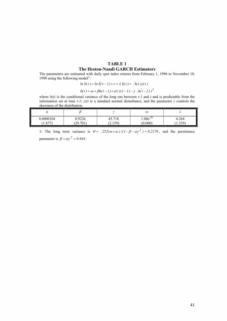
41

TABLE 1 The Heston-Nandi GARCH Estimators

The parameters are estimated with daily spot index returns from February 1, 1996 to November 10, 1998 using the following model1/:

2))1t(h)1t(z()1t(h)t(h

)t(z)t(h)t(h r)1t(Sln)t(Sln

−−−+−+=

+++−=

γαβω

λ

where h(t) is the conditional variance of the long run between t-1 and t and is predictable from the information set at time t-1; z(t) is a standard normal disturbance, and the parameter γ controls the skewness of the distribution.

α β γ ω λ

0.0000104 (1.877)

0.9226 (29.701)

45.718 (2.159)

1.00e-20 (0.000)

4.264 (1.339)

1/ The long term variance is 2170.0)1/()(252 2 =−−+= αγβαωθ , and the persistence

parameter is 944.02 =+αγβ .

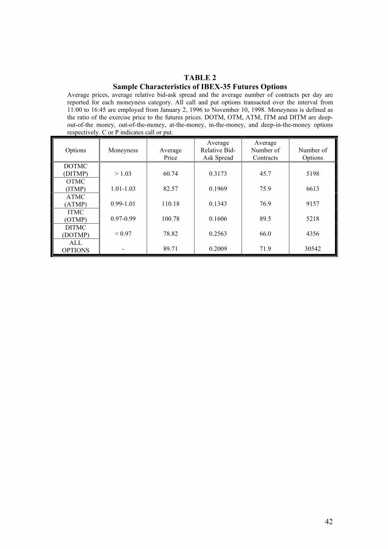
42

TABLE 2 Sample Characteristics of IBEX-35 Futures Options

Average prices, average relative bid-ask spread and the average number of contracts per day are reported for each moneyness category. All call and put options transacted over the interval from 11:00 to 16:45 are employed from January 2, 1996 to November 10, 1998. Moneyness is defined as the ratio of the exercise price to the futures prices. DOTM, OTM, ATM, ITM and DITM are deep-out-of-the money, out-of-the-money, at-the-money, in-the-money, and deep-in-the-money options respectively. C or P indicates call or put.

Options

Moneyness

Average

Price

Average Relative Bid-Ask Spread

Average Number of Contracts

Number of

Options DOTMC (DITMP) OTMC (ITMP) ATMC

(ATMP) ITMC

(OTMP) DITMC

(DOTMP) ALL

OPTIONS

> 1.03

1.01-1.03

0.99-1.01

0.97-0.99

< 0.97

-

60.74

82.57

110.18

100.78

78.82

89.71

0.3173

0.1969

0.1343

0.1606

0.2563

0.2009

45.7

75.9

76.9

89.5

66.0

71.9

5198

6613

9157

5218

4356

30542

43

TABLE 3 Daily In-Sample Pricing Performance of Alternative Option Pricing Models for

Calls and Puts BS is the Black-Scholes model; NP(X) is the semiparametric option model, where the volatility function is estimated nonparametrically for each day from January 2, 1996 to November 10, 1998 using all available call/put options transacted from 11:00 to 16:45, and considering only the exercise price as an explanatory variable. The call/put price is calculated by using the BS pricing function evaluated at the contemporaneous (nonparametrically) estimated volatility; NP(X, SP) is a similar price except that the nonparametric estimated volatility includes not only the exercise price but also the bid-ask spread of each option as a proxy for liquidity; Ad-hoc BS is a version of the BS model with exercise specific implied volatility; HN is the closed-form GARCH model proposed by Heston and Nandi (2000) estimated with an updated asymmetric GARCH. The statistical performance for the pricing errors is assessed by analyzing the proportion of theoretical prices lying outside their bid-ask spread boundaries; that is, Prob [Price model ∉ (Bid, Ask)]. In each case we report the corresponding proportion for a given model and, in parentheses, the identifying number of the competing model that has a significantly higher proportion than the model being analyzed according to our Z-statistics at the 5% level. OTM, ATM, ITM are out-of-the-money, at-the-money, in-the-money options respectively. X is the exercise price, and SP is the relative bid-ask spread.

1996-1998 CALLS

BS (1)

NP(X) (2)

NP(X, SP) (3)

Ad-hoc BS (4)

HN (5)

ALL 0.470 Z(5)

0.205 Z(1,5)

0.164 Z(1,2,4,5)

0.180 Z(1,2,5)

0.579 Z(-)

OTM 0.455 Z(5)

0.211 Z(1,5)

0.160 Z(1,2,4,5)

0.190 Z(1,2,5)

0.631 Z(-)

ATM 0.456 Z(5)

0.195 Z(1,5)

0.180 Z(1,2,5)

0.169 Z(1,2,3,5)

0.528 Z(-)

ITM 0.470 Z(-)

0.200 Z(1,5)

0.137 Z(1,2,4,5)

0.157 Z(1,2,5)

0.428 Z(1)

1996-1998 PUTS

BS (1)

NP(X) (2)

NP(X, SP) (3)

Ad-hoc BS (4)

HN (5)

ALL 0.471 Z(5)

0.252 Z(1,5)

0.181 Z(1,2,4,5)

0.200 Z(1,2,5)

0.555 Z(-)

OTM 0.499 Z(5)

0.271 Z(1,5)

0.186 Z(1,2,4,5)

0.208 Z(1,2,5)

0.541 Z(-)

ATM 0.394 Z(5)

0.217 Z(1,5)

0.164 Z(1,2,4,5)

0.190 Z(1,2,5)

0.579 Z(-)

ITM 0.517 Z(5)

0.213 Z(1,5)

0.158 Z(1,2,4,5)

0.197 Z(1,5)

0.595 Z(-)

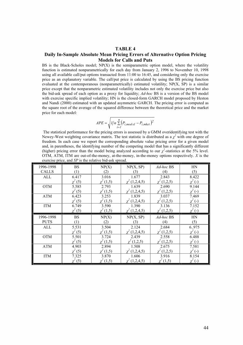
44

TABLE 4 Daily In-Sample Absolute Mean Pricing Errors of Alternative Option Pricing

Models for Calls and Puts BS is the Black-Scholes model; NP(X) is the semiparametric option model, where the volatility function is estimated nonparametrically for each day from January 2, 1996 to November 10, 1998 using all available call/put options transacted from 11:00 to 16:45, and considering only the exercise price as an explanatory variable. The call/put price is calculated by using the BS pricing function evaluated at the contemporanous (nonparametrically) estimated volatility; NP(X, SP) is a similar price except that the nonparametric estimated volatility includes not only the exercise price but also the bid-ask spread of each option as a proxy for liquidity; Ad-hoc BS is a version of the BS model with exercise specific implied volatility; HN is the closed-form GARCH model proposed by Heston and Nandi (2000) estimated with an updated asymmetric GARCH. The pricing error is computed as the square root of the average of the squared difference between the theoretical price and the market price for each model:

( )∑ −==

n

1i

2mket,ielmod,i PPn1APE

The statistical performance for the pricing errors is assessed by a GMM overidentifying test with the Newey-West weighting covariance matrix. The test statistic is distributed as a χ2 with one degree of freedom. In each case we report the corresponding absolute value pricing error for a given model and, in parentheses, the identifying number of the competing model that has a significantly different (higher) pricing error than the model being analyzed according to our χ2-statistics at the 5% level. OTM, ATM, ITM are out-of-the-money, at-the-money, in-the-money options respectively. X is the exercise price, and SP is the relative bid-ask spread.

1996-1998 CALLS

BS (1)

NP(X) (2)

NP(X, SP) (3)

Ad-hoc BS (4)

HN (5)

ALL 6.417 χ2 (5)

3.016 χ2 (1,5)

1.677 χ2 (1,2,4,5)

2.843 χ2 (1,2,5)

8.422 χ2 (-)

OTM 5.585 χ2 (5)

2.793 χ2 (1,5)

1.639 χ2 (1,2,4,5)

2.690 χ2 (1,2,5)

9.144 χ2 (-)

ATM 6.423 χ2 (5)

3.253 χ2 (1,5)

1.839 χ2 (1,2,4,5)

3.037 χ2 (1,2,5)

7.469 χ2 (-)

ITM 6.749 χ2 (5)

3.590 χ2 (1,5)

1.390 χ2 (1,2,4,5)

3.136 χ2 (1,2,5)

7.152 χ2 (-)

1996-1998 PUTS

BS (1)

NP(X) (2)

NP(X, SP) (3)

Ad-hoc BS (4)

HN (5)

ALL 5.531 χ2 (5)

3.504 χ2 (1,5)

2.124 χ2 (1,2,4,5)

2.684 χ2 (1,2,5)

6..975 χ2 (-)

OTM 5.501 χ2 (5)

3.724 χ2 (1,5)

2.439 χ2 (1,2,5)

2.558 χ2 (1,2,5)

6.488 χ2 (-)

ATM 4.903 χ2 (5)

2.894 χ2 (1,5)

1.508 χ2 (1,2,4,5)

2.675 χ2 (1,2,5)

7.581 χ2 (-)

ITM 7.325 χ2 (5)

3.870 χ2 (1,5)

1.606 χ2 (1,2,4,5)

3.916 χ2 (1,5)

8.154 χ2 (-)

45

TABLE 5 Daily Out-of-Sample Pricing Performance of Alternative Option Pricing

Models for Calls and Puts BS is the Black-Scholes model; NP(X) is the semiparametric option model, where the volatility function is estimated nonparametrically for each day from January 2, 1996 to November 10, 1998 using all available call/put options transacted from 11:00 to 16:45, and considering only the exercise price as an explanatory variable. The call/put price is calculated by using the BS pricing function evaluated at the previously (nonparametrically) estimated volatility; NP(X, SP) is a similar price except that the nonparametric estimated volatility includes not only the exercise price but also the bid-ask spread of each option as a proxy for liquidity; Ad-hoc BS is a version of the BS model with exercise specific implied volatility; HN is the closed-form GARCH model proposed by Heston and Nandi (2000) estimated with an updated asymmetric GARCH. The statistical performance for the pricing errors is assessed by analyzing the proportion of theoretical prices lying outside their bid-ask spread boundaries; that is, Prob [Price model ∉ (Bid, Ask)]. In each case we report the corresponding proportion for a given model and, in parentheses, the identifying number of the competing model that has a significantly higher proportion than the model being analyzed according to our Z-statistics at the 5% level. OTM, ATM, ITM are out-of-the-money, at-the-money, in-the-money options respectively. X is the exercise price, and SP is the relative bid-ask spread.

1996-1998 CALLS

BS (1)

NP(X) (2)

NP(X, SP) (3)

Ad-hoc BS (4)

HN (5)

ALL 0.516 Z(5)

0.418 Z(1,3,5)

0.447 Z(1,5)

0.410 Z(1,2,3,5)

0.657 Z(-)

OTM 0.579 Z(5)

0.461 Z(1,3,5)

0.479 Z(1,5)

0.456 Z(1,2*,3,5)

0.709 Z(-)

ATM 0.419 Z(5)

0.375 Z(1,3,5)

0.406 Z(1,5)

0.356 Z(1,2,3,5)

0.618 Z(-)

ITM 0.446 Z(5*)

0.302 Z(1,3,5)

0.383 Z(1,5)

0.304 Z(1,3,5)

0.469 Z(-)

1996-1998 PUTS

BS (1)

NP(X) (2)

NP(X, SP) (3)

Ad-hoc BS (4)

HN (5)

ALL 0.565 Z(5)

0.424 Z(1,3,5)

0.504 Z(1,5)

0.396 Z(1,2,3,5)

0.614 Z(-)

OTM 0.588 Z(-)

0.446 Z(1,3,5)

0.520 Z(1,5)

0.412 Z(1,2,3,5)

0.594 Z(-)

ATM 0.520 Z(5)

0.372 Z(1,3,5)

0.476 Z(1,5)

0.358 Z(1,2,3,5)

0.651 Z(-)

ITM 0.527 Z(5)

0.422 Z(1,3,5)

0.461 Z(1,5)

0.405 Z(1,3,5)

0.655 Z(-)

* means significantly higher at the 10% rather than the otherwise reported 5% level

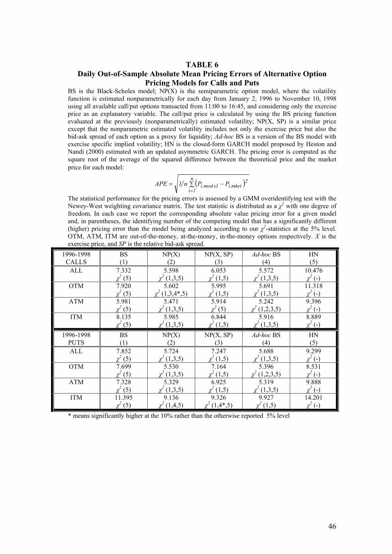
46

TABLE 6 Daily Out-of-Sample Absolute Mean Pricing Errors of Alternative Option

Pricing Models for Calls and Puts BS is the Black-Scholes model; NP(X) is the semiparametric option model, where the volatility function is estimated nonparametrically for each day from January 2, 1996 to November 10, 1998 using all available call/put options transacted from 11:00 to 16:45, and considering only the exercise price as an explanatory variable. The call/put price is calculated by using the BS pricing function evaluated at the previously (nonparametrically) estimated volatility; NP(X, SP) is a similar price except that the nonparametric estimated volatility includes not only the exercise price but also the bid-ask spread of each option as a proxy for liquidity; Ad-hoc BS is a version of the BS model with exercise specific implied volatility; HN is the closed-form GARCH model proposed by Heston and Nandi (2000) estimated with an updated asymmetric GARCH. The pricing error is computed as the square root of the average of the squared difference between the theoretical price and the market price for each model:

( )∑ −==

n

1i

2mket,ielmod,i PPn1APE

The statistical performance for the pricing errors is assessed by a GMM overidentifying test with the Newey-West weighting covariance matrix. The test statistic is distributed as a χ2 with one degree of freedom. In each case we report the corresponding absolute value pricing error for a given model and, in parentheses, the identifying number of the competing model that has a significantly different (higher) pricing error than the model being analyzed according to our χ2-statistics at the 5% level. OTM, ATM, ITM are out-of-the-money, at-the-money, in-the-money options respectively. X is the exercise price, and SP is the relative bid-ask spread.

1996-1998 CALLS

BS (1)

NP(X) (2)

NP(X, SP) (3)

Ad-hoc BS (4)

HN (5)

ALL 7.332 χ2 (5)

5.598 χ2 (1,3,5)

6.053 χ2 (1,5)

5.572 χ2 (1,3,5)

10.476 χ2 (-)

OTM 7.920 χ2 (5)

5.602 χ2 (1,3,4*,5)

5.995 χ2 (1,5)

5.691 χ2 (1,3,5)

11.318 χ2 (-)

ATM 5.981 χ2 (5)

5.471 χ2 (1,3,5)

5.914 χ2 (5)

5.242 χ2 (1,2,3,5)

9.396 χ2 (-)

ITM 8.135 χ2 (5)

5.985 χ2 (1,3,5)

6.844 χ2 (1,5)

5.916 χ2 (1,3,5)

8.889 χ2 (-)

1996-1998 PUTS

BS (1)

NP(X) (2)

NP(X, SP) (3)

Ad-hoc BS (4)

HN (5)

ALL 7.852 χ2 (5)

5.724 χ2 (1,3,5)

7.247 χ2 (1,5)

5.688 χ2 (1,3,5)

9.299 χ2 (-)

OTM 7.699 χ2 (5)

5.530 χ2 (1,3,5)

7.164 χ2 (1,5)

5.396 χ2 (1,2,3,5)

8.531 χ2 (-)

ATM 7.328 χ2 (5)

5.329 χ2 (1,3,5)

6.925 χ2 (1,5)

5.319 χ2 (1,3,5)

9.888 χ2 (-)

ITM 11.395 χ2 (5)

9.136 χ2 (1,4,5)

9.326 χ2 (1,4*,5)

9.927 χ2 (1,5)

14.201 χ2 (-)

* means significantly higher at the 10% rather than the otherwise reported 5% level

47

TABLE 7 Daily Hedging Errors of Alternative Option Pricing Models for Calls and Puts

BS is the Black-Scholes model; NP(X) is the semiparametric option model, where the volatility function is estimated nonparametrically for each day from January 2, 1996 to November 10, 1998 using all available call/put options transacted from 11:00 to 16:45, and considering only the exercise price as an explanatory variable. The call/put price is calculated by using the BS pricing function evaluated at the previously (nonparametrically) estimated volatility; NP(X, SP) is a similar price except that the nonparametric estimated volatility includes not only the exercise price but also the bid-ask spread of each option as a proxy for liquidity; Ad-hoc BS is a version of the BS model with exercise specific implied volatility; HN is the closed-form GARCH model proposed by Heston and Nandi (2000) estimated with an updated asymmetric GARCH. The statistical performance of the hedging errors is assessed by a GMM overidentifying test with the Newey-West weighting covariance matrix. The test statistic is distributed as a χ2 with one degree of freedom. In each case we report the corresponding mean hedging error for a given model and, in parentheses, the identifying number of the competing model that has a significantly different (higher) mean hedging error than the model being analyzed according to our χ2-statistics at the 5% level. OTM, ATM, ITM are out-of-the-money, at-the-money, in-the-money options respectively. X is the exercise price, and SP is the relative bid-ask spread.

1996-1998 CALLS

BS (1)

NP(X) (2)

NP(X, SP) (3)

Ad-hoc BS (4)

HN (5)

ALL 11.694 χ2 (5)

10.038 χ2 (1,3,4,5)

10.170 χ2 (1,5)

10.122 χ2 (1,3,5)

24.549 χ2 (-)

OTM 14.101 χ2 (5)

11.516 χ2 (1,3,4*,5)

11.816 χ2 (1,5)

11.571 χ2 (1,3,5)

26.792 χ2 (-)

ATM 8.300 χ2 (5)

8.013 χ2 (4*,5)

7.951 χ2 (1,2,4,5)

8.089 χ2 (5)

24.333 χ2 (-)

ITM 7.302 χ2 (4,5)

7.123 χ2 (1,4*,5)

6.800 χ2 (1,4,5)

7.440 χ2 (-)

9.846 χ2 (-)

1996-1998 PUTS

BS (1)

NP(X) (2)

NP(X, SP) (3)

Ad-hoc BS (4)

HN (5)

ALL 10.430 χ2 (3,5)

8.512 χ2 (1,3,5)

10.635 χ2 (5)

8.757 χ2 (1,3,5)

40.387 χ2 (-)

OTM 10.587 χ2 (3,5)

8.766 χ2 (1,3,5)

11.105 χ2 (5)

9.219 χ2 (1,3,5)

35.032 χ2 (-)

ATM 9.856 χ2 (5)

7.317 χ2 (1,3,5)

9.264 χ2 (5)

7.564 χ2 (1,3,5)

37.471 χ2 (-)

ITM 11.030 χ2 (5)

10.378 χ2 (5)

11.290 χ2 (5)

8.884 χ2 (1,5)

44.511 χ2 (-)

* means significantly higher at the 10% rather than the otherwise reported 5% level

48

TABLE 8 Percentage Pricing Errors and Explanatory Variables

BS is the Black-Scholes model; NP(X) is the semiparametric option model, where the volatility function is estimated nonparametrically for each day from January 2, 1996 to November 10, 1998 using all available call/put options transacted from 11:00 to 16:45, and considering only the exercise price as an explanatory variable. The call/put price is calculated by using the BS pricing function evaluated at the previously (nonparametrically) estimated volatility; NP(X, SP) is a similar price except that the nonparametric estimated volatility includes not only the exercise price but also the bid-ask spread of each option as a proxy for liquidity; Ad-hoc BS is a version of the BS model with exercise specific implied volatility; HN is the closed-form GARCH model proposed by Heston and Nandi (2000) estimated with an updated asymmetric GARCH. X is the exercise price, and SP is the relative bid-ask spread. For a given option pricing model, the following regression is employed to explain the percentage pricing errors of all call/put options transacted in our sample:

itit6it5t4t3t2it1it SPbXlnbKUbSKbbbae εστ +++++++= where for the ith option at date t, ite is the percentage pricing error defined as the difference between the theoretical price and the market price divided by the market price; itτ the time to maturity;

itX the exercise price and itSP the bid-ask spread. tt SK,σ and tKU are respectively the daily volatility, skewness and (excess) kurtosis. P-values in parentheses.

1996-1998 CALLS

BS (1)

NP(X) (2)

NP(X, SP) (3)

Ad-hoc BS (4)

HN (5)

Intercept -1.069 (0.000)

-0.173 (0.000)

-0.209 (0.000)

-0.049 (0.268)

-0.050 (0.680)

Time to maturity

0.562 (0.000)

-0.031 (0.586)

-0.114 (0.065)

-0.082 (0.187)

3.420 (0.000)

Volatility -0.455 (0.000)

-0.163 (0.000)

-0.169 (0.000)

-0.115 (0.000)

-0.997 (0.000)

Skewness -0.041 (0.000)

-0.019 (0.000)

-0.019 (0.000)

-0.015 (0.000)

-0.008 (0.000)

Kurtosis -0.001 (0.536)

-0.000 (0.705)

0.001 (0.291)

0.003 (0.002)

0.004 (0.157)

Ln Exercise 0.124 (0.000)

0.020 (0.000)

0.024 (0.000)

0.005 (0.323)

-0.001 (0.945)

Spread 0.212 (0.000)

0.057 (0.000)

0.080 (0.000)

0.062 (0.000)

0.785 (0.000)

1996-1998 PUTS

BS (1)

NP(X) (2)

NP(X, SP) (3)

Ad-hoc BS (4)

HN (5)

Intercept -0.279 (0.000)

-0.657 (0.000)

-0.886 (0.000)

-0.335 (0.000)

0.597 (0.000)

Time to maturity

-0.496 (0.000)

-0.036 (0.601)

-0.294 (0.000)

0.183 (0.016)

1.737 (0.000)

Volatility -0.200 (0.000)

-0.119 (0.000)

-0.137 (0.000)

-0.064 (0.007)

-0.619 (0.000)

Skewness 0.021 (0.000)

0.032 (0.000)

0.035 (0.000)

0.049 (0.000)

0.045 (0.000)

Kurtosis -0.003 (0.003)

-0.004 (0.000)

-0.004 (0.005)

-0.001 (0.248)

-0.001 (0.620)

Ln Exercise 0.041 (0.000)

0.082 (0.000)

0.112 (0.000)

0.043 (0.000)

-0.065 (0.000)

Spread -0.299 (0.000)

-0.069 (0.000)

-0.072 (0.000)

-0.014 (0.122)

0.146 (0.000)

49

FIGURE 1

Daily Annualized Volatilities: Heston & Nandi vs. Implied Volatility

1996-1998

0

10

20

30

40

50

60

70

1 48 95 142 189 236 283 330 377 424 471 518 565

Time

Vol

atili

ty Volatility H&NImplied Volatility