Performance of a Hot-Dry Climate Whole-House Retrofit E. Weitzel, A. German, and E. Porse Alliance for Residential Building Innovation

June 2014

NOTICE

This report was prepared as an account of work sponsored by an agency of the United States government. Neither the United States government nor any agency thereof, nor any of their employees, subcontractors, or affiliated partners makes any warranty, express or implied, or assumes any legal liability or responsibility for the accuracy, completeness, or usefulness of any information, apparatus, product, or process disclosed, or represents that its use would not infringe privately owned rights. Reference herein to any specific commercial product, process, or service by trade name, trademark, manufacturer, or otherwise does not necessarily constitute or imply its endorsement, recommendation, or favoring by the United States government or any agency thereof. The views and opinions of authors expressed herein do not necessarily state or reflect those of the United States government or any agency thereof.

Available electronically at http://www.osti.gov/scitech

Available for a processing fee to U.S. Department of Energy and its contractors, in paper, from:

U.S. Department of Energy Office of Scientific and Technical Information

P.O. Box 62 Oak Ridge, TN 37831-0062

phone: 865.576.8401 fax: 865.576.5728

email: mailto:reports@adonis.osti.gov

Available for sale to the public, in paper, from: U.S. Department of Commerce

National Technical Information Service 5285 Port Royal Road Springfield, VA 22161 phone: 800.553.6847

fax: 703.605.6900 email: orders@ntis.fedworld.gov

online ordering: http://www.ntis.gov/ordering.htm

Printed on paper containing at least 50% wastepaper, including 20% postconsumer waste

iii

Performance of a Hot-Dry Climate Whole-House Retrofit

Prepared for:

The National Renewable Energy Laboratory

On behalf of the U.S. Department of Energy’s Building America Program

Office of Energy Efficiency and Renewable Energy

15013 Denver West Parkway

Golden, CO 80401

NREL Contract No. DE-AC36-08GO28308

Prepared by:

Elizabeth Weitzel

Alliance for Residential Building Innovation (ARBI)

Davis Energy Group, Team Lead

123 C Street

Davis, California 95616

NREL Technical Monitor: Michael Gestwick

Prepared under Subcontract No. KNDJ-0-40340-03

June 2014

iv

[This page left blank]

v

Contents List of Figures ............................................................................................................................................ vi List of Tables .............................................................................................................................................. vi Definitions .................................................................................................................................................. vii Acknowledgments ..................................................................................................................................... ix Executive Summary .................................................................................................................................... x 1 Introduction ........................................................................................................................................... 1

1.1 Background ..........................................................................................................................1 1.2 Research Questions ..............................................................................................................2

2 Characterization of Site and Retrofit Measures ................................................................................ 3 2.1 Residence Description .........................................................................................................3 2.2 Retrofit Measure Options and Details..................................................................................4 2.3 Preliminary Savings Estimations .........................................................................................8

3 Evaluation Methodology .................................................................................................................... 10 3.1 General Technical Approach .............................................................................................10 3.2 Measurements ....................................................................................................................10

3.2.1 Short-Term Tests ...................................................................................................10 3.2.2 Monitoring Points ..................................................................................................10

3.3 Utility Bill Disaggregation and Model Calibration ...........................................................11 4 Results and Discussion ..................................................................................................................... 13

4.1 Short-Term Test Results ....................................................................................................13 4.2 System Commissioning .....................................................................................................13 4.3 Annual Energy Use ............................................................................................................14 4.4 Project Economics .............................................................................................................18 4.5 Homeowner Feedback .......................................................................................................19

5 Conclusions and Recommendations ............................................................................................... 22 References ................................................................................................................................................. 24 Appendix: Homeowner Survey ................................................................................................................ 25

vi

List of Figures Figure 1. Front view of Stockton house .................................................................................................... 3 Figure 2. BEopt optimization curve ........................................................................................................... 6 Figure 3. Assumed seasonal effect on water heating loads ................................................................. 12 Figure 4. Natural gas usage (pre- and post-retrofit) .............................................................................. 14 Figure 5. Electrical energy usage (pre- and post-retrofit) ..................................................................... 15 Figure 6. Monthly calculated source energy savings from utility bill ................................................. 17 Figure 7. Normalized source energy savings (TMY3) ........................................................................... 17 Figure 8. Winter comfort levels ............................................................................................................... 20 Figure 9. Summer comfort levels ............................................................................................................ 20

Unless otherwise noted, all figures were created by the ARBI team. List of Tables Table 1. Building Energy Efficiency Improvements ................................................................................ 4 Table 2. Measure Incremental Costs ......................................................................................................... 5 Table 3. BEopt Projected Annual Site Energy Use of the Pre-Retrofit and Post-Retrofit Building .... 8 Table 4. BEopt Projected Annual Source Energy for the Pre-Retrofit and Post-Retrofit Building ..... 9 Table 5. Measurement Point List ............................................................................................................. 11 Table 6. Sensor Specifications ................................................................................................................ 11 Table 7. Short-Term Diagnostic Test Results ........................................................................................ 13 Table 8. Characterization of Pre- and Post-Retrofit Weather, Projected Energy Use, and Costs .... 16 Table 9. Projected Savings and Cost Effectiveness .............................................................................. 18 Table 10. Comparison of Standard and Whole-House Retrofit Package Savings and Economics .. 19

Unless otherwise noted, all tables were created by the ARBI team.

vii

Definitions

ACCA Air Conditioning Contractors of America

ACH50 Air changes per hour at a pressure difference of 50 Pascal

AFUE Annual Fuel Utilization Efficiency

ARBI Alliance for Residential Building Innovation

ASHRAE American Society for Heating, Refrigerating and Air Conditioning Engineers

BEopt™ Building Energy Optimization simulation

Btu British Thermal Units

CDD Cooling Degree Day

CFL Compact Fluorescent Lamp

CFM Cubic feet per minute

CFM50 Cubic feet per minute at a pressure differential of 50 Pascal

DEG Davis Energy Group, Inc.

EER Energy Efficiency Ratio

EF Energy Factor

GHS Green Home Solutions by Grupe

HDD Heating Degree Day

HEU Home Energy Upgrade

HVAC Heating, Ventilation, and Air Conditioning

kWh Kilowatt-hour

MEL Miscellaneous Electric Load

RH Relative Humidity (%)

RTD Resistive temperature device

SCFM Standard cubic feet per minute

viii

SEER Seasonal Energy Efficiency Ratio

SHGC Solar Heat Gain Coefficient

TMY3 Typical Meteorological Year 3

UV Ultraviolet

ix

Acknowledgments

Davis Energy Group would like to acknowledge the U.S. Department of Energy Building America Program for its funding and support of this research effort. In addition, we would like to thank Green Home Solutions, for its cooperation and coordination throughout all stages of this project.

x

Executive Summary

The Stockton house retrofit is a two-story Tudor style single-family home located in Stockton, California. Although classified as a hot-dry climate region, Stockton generally has relatively mild summers due to its proximity to the San Joaquin Delta that brings in cool night-time breezes from the San Francisco Bay Area. The homeowners completed a whole-house energy retrofit under a Stockton area Large-Scale Retrofit Program administered by the Alliance for Residential Building Innovation (ARBI). The implemented retrofit package included:

• Heating, ventilation, and air conditioning, water heater, and window replacements

• Duct sealing

• Adding attic and floor insulation

• Envelope sealing

• Domestic hot water pipe insulation

• Compact fluorescent lamp replacements

• Mechanical ventilation upgrades.

The objective of this work is to expand the level of understanding of whole-house retrofit impacts in climates where lighting and miscellaneous electric loads represent a large fraction of annual energy consumption. In many climates with high space conditioning loads, whole-house retrofits can demonstrate significant operating cost savings and favorable economics through the reduction of space conditioning energy consumption. In milder climates, similar to that of Stockton, whole-house retrofits represent an opportunity to evaluate overall performance and cost-effectiveness, and to develop findings that will assist future efforts. This information is important for the home energy retrofit industry as it gains a better understanding of cost and performance tradeoffs in a range of applications and climates.

Source energy savings (normalized to a Typical Meteorological Year’s weather data, TMY3) with the whole-house retrofit were estimated at 23% compared to the pre-retrofit case, or 15 percentage points higher than the projected 8% savings identified for the basic package of measures typically implemented in the Large-Scale Retrofit Program project1. Projected (TMY3) annual energy savings totaling 1,377 kWh and 295 therms/year were largely a result of the water heater upgrade and reduced furnace heating consumption (improved furnace efficiency and load reduction benefits due to envelope sealing, added insulation, and duct sealing). Savings were considerably lower than the 47% savings identified with BEopt modeling, primarily due to very low cooling energy usage and much higher than typical miscellaneous electric loads (representing 40% of annual source energy in the Stockton house). The economics could not generate a favorable cash flow for the standard package of measures due to high financed costs and lower than typical heating, ventilation, and air conditioning system operation. This whole-

1 Standard package includes R-49 attic insulation, duct replacement, envelope sealing, hot-water pipe insulation, water heater blanket, lighting upgrade to high efficacy lamps, low-flush toilet upgrade, and mechanical ventilation upgrade.

xi

house retrofit package promised additional utility savings, but could not bridge the gap of cost effectiveness.

Despite the lower than expected savings, the homeowner expressed a high degree of satisfaction with the retrofit and the improved comfort. The project highlighted the complexities that occur in implementing projects that go beyond the simple envelope/duct sealing and attic insulation steps. The more complicated whole-house retrofits must integrate homeowner priorities, as well as deal with more costly implementation issues. In this specific case, a window retrofit was a high priority for the homeowner, despite the $11,000 cost and poor economics. Mild climate whole-house retrofits are challenged by reduced paybacks for many measures. Learning how to maximize the cost effectiveness of whole-house energy retrofits and developing a viable approach to addressing miscellaneous energy use are key needs for developing effective retrofit strategies.

1

1 Introduction

1.1 Background The Stockton (California) House retrofit is part of The Energy Challenge in Stockton project. This pilot project is administered by Davis Energy Group (DEG) and funded by the California Energy Commission and the Alliance for Residential Building Innovation (ARBI) team for Building America. The Large-Scale Retrofit Program pilot project primary objective is to increase energy efficiency in the residential sector through improved uptake of whole-house Home Energy Upgrades (HEUs). The Energy Challenge aims to develop a market for energy efficiency retrofits through consumer outreach and education, identification of market efficiencies, and promotion of HEUs in the marketplace. The pilot uses a deemed cost-effective Standard Package of energy efficiency measures consisting of the following:

• R-49 attic insulation

• Duct replacement

• Envelope sealing

• Hot-water pipe insulation

• Water heater blanket

• Lighting upgrade to high efficacy lamps

• Low-flush toilet upgrade

• Mechanical ventilation upgrade.

The Standard Package is designed to meet annual site energy savings of 25% and cost participants $9,456 ($6,706 after rebates and incentives). A comprehensive “whole-house” retrofit would include additional measures (e.g., heating, ventilation, and air conditioning [HVAC] equipment replacement and/or window replacement), generating additional energy savings and thermal comfort, but at a higher cost and tailored to the individual home. Although the Energy Challenge in Stockton has successfully marketed Standard Package HEUs with more than 165 retrofits completed to date, the Stockton House whole-house retrofit project is one of the few HEUs implemented that includes additional energy efficiency measures. Thus, the Stockton House offers a unique opportunity to study and document the energy performance and cost effectiveness of the more complicated retrofit savings, as well as gauge occupant satisfaction. Results can inform program design and marketing activities, including efforts to develop more effective incentives to homeowners participating in the HEU process. Previous research has identified early adopters as an important tool in encouraging broader implementation of retrofit programs within a neighborhood (Berman et al. 2012).

For the Stockton House whole-house retrofit project, homeowner dissatisfaction with existing energy bills and overall comfort were key motivators for pursuing the whole-house retrofit. The link between energy efficiency, increased occupant satisfaction, and enhanced home resale price is a potentially powerful marketing tool that is just beginning to gain recognition (Kok and Kahn 2012). Identifying cost-optimized climate appropriate packages through detailed modeling (Fairey and Parker 2012) is a valuable step in the evolution of the HEU industry, but the

2

implementation and documentation of projects such as this are also needed to develop case studies that inform stakeholders and the broader public on how implementation may be impacted by site constraints, homeowner input, and available financial resources.

1.2 Research Questions The following research questions were explored in this study:

1. Are there measured savings and homeowner comfort benefits resulting from whole-house retrofits that may motivate homeowners to invest more in whole-house retrofits as opposed to more standard upgrades?

2. What energy upgrade strategies are most effective (in terms of cost and energy savings) in whole-house retrofit projects?

The study used a combination of pre- and post-retrofit energy simulations to predict energy savings, monitoring of site energy use to document end use performance, and an assessment of homeowner feedback to determine qualitative response to the retrofit activities.

3

2 Characterization of Site and Retrofit Measures

2.1 Residence Description The Stockton House is a two-story, Tudor-style single-family home located in Stockton, California (Figure 1), approximately 90 miles east of San Francisco. Although the climate is defined as Hot-Dry by Building America conventions,2 the summer climate is considerably more moderate than much of California’s central valley, due to the proximity to the San Francisco Bay Area. Based on Typical Meteorological Year (TMY3)3 data, Stockton experiences an average of 2,494 heating degree days (HDDs) and 1,295 cooling degree days (CDDs), on a 65°F base.

Figure 1. Front view of Stockton house

The 2,152-ft2 home was originally built in 1939 and is currently occupied by an adult couple. The house has a combined raised floor and partial basement foundation. Table 1 summarizes the pre-retrofit conditions and the energy efficiency improvements implemented as part of the whole-house retrofit.

2 and climate zone 3B by the International Energy Conservation Code. 3 Statistics for USA_CA_Stockton.Metro.AP.724920_TMY3 http://apps1.eere.energy.gov/buildings/energyplus/cfm/weather_data3.cfm/region=4_north_and_central_america_wmo_region_4/country=1_usa/cname=USA#CA

4

Table 1. Building Energy Efficiency Improvements

Measure Pre-Retrofit Post-Retrofit Basic Building Characteristics

Building Type/Stories Single-family, 2-story, partial basement

Single-family, 2 story, partial basement

Conditioned Floor Area 2,152 2,152 Number of Bedrooms 3 3

Envelope Attic Vented, R-11 Vented, R-49 Roof

Wall Insulation Tile

None Tile

None Raised Floor Insulation None R-19

Framing Standard 2 × 4, 16 in. o.c. Standard 2 × 4, 16 in. o.c. Glazing Properties

Window Type Metal single pane Vinyl dual pane U-Value/SHGCa 1.28/0.80 0.30/0.30

HVAC Equipment Heating System Type and

Rated Efficiency Natural gas (64% AFUEb) Single speed, 105 kBtu/h

Natural gas (95% AFUE) Two speed, 64–92 kBtu/h

Cooling System Type and Rated Efficiency 8 SEERc/7.7 EERd 16 SEER/12 EER

Ventilation Ducting

Kitchen and one bath fan R-2.1

Kitchen and two bath fans Crawlspace and attic R-8,

Interstitial space R-2.1 Water Heating Equipment

Water Heater Type and Efficiency Natural gas storage 0.62 EFe Condensing tankless-

Natural gas 0.96 EF Tank Capacity/Gallons 40,000 Btu/h 50 gal 15,000 - 150,000 Btu/h

Appliances and Lighting

Appliances ENERGY STAR clothes washer, dryer

ENERGY STAR clothes washer, dryer

Dryer Fuel Electric Electric Oven/Range Fuel Natural gas Natural gas

Lighting 100% CFLf 100% CFL a Solar heat gain coefficient b Annual fuel utilization efficiency c Seasonal energy efficiency ratio d Energy efficiency ratio e Energy factor f Compact fluorescent lamp 2.2 Retrofit Measure Options and Details The Stockton House retrofit opportunity was identified and executed by Building America Partner Green Home Solutions by Grupe (GHS). Construction work was completed early fall 2011. Cost data provided by GHS indicated total upgrade costs of $38,000. Table 2 summarizes the installed retrofit measures and their associated costs. The incremental cost for the new

5

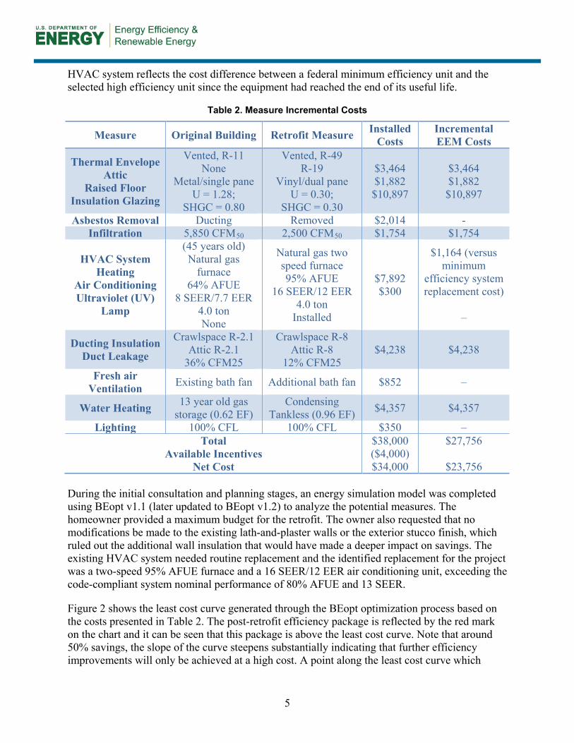
HVAC system reflects the cost difference between a federal minimum efficiency unit and the selected high efficiency unit since the equipment had reached the end of its useful life.

Table 2. Measure Incremental Costs

Measure Original Building Retrofit Measure Installed Costs

Incremental EEM Costs

Thermal Envelope Attic

Raised Floor Insulation Glazing

Vented, R-11 None

Metal/single pane U = 1.28;

SHGC = 0.80

Vented, R-49 R-19

Vinyl/dual pane U = 0.30;

SHGC = 0.30

$3,464 $1,882 $10,897

$3,464 $1,882 $10,897

Asbestos Removal Ducting Removed $2,014 - Infiltration 5,850 CFM50 2,500 CFM50 $1,754 $1,754

HVAC System Heating

Air Conditioning Ultraviolet (UV)

Lamp

(45 years old) Natural gas

furnace 64% AFUE

8 SEER/7.7 EER 4.0 ton None

Natural gas two speed furnace 95% AFUE

16 SEER/12 EER 4.0 ton

Installed

$7,892 $300

$1,164 (versus minimum

efficiency system replacement cost)

–

Ducting Insulation Duct Leakage

Crawlspace R-2.1 Attic R-2.1

36% CFM25

Crawlspace R-8 Attic R-8

12% CFM25 $4,238 $4,238

Fresh air Ventilation Existing bath fan Additional bath fan $852 –

Water Heating 13 year old gas storage (0.62 EF)

Condensing Tankless (0.96 EF) $4,357 $4,357

Lighting 100% CFL 100% CFL $350 – Total

Available Incentives Net Cost

$38,000 ($4,000) $34,000

$27,756

$23,756 During the initial consultation and planning stages, an energy simulation model was completed using BEopt v1.1 (later updated to BEopt v1.2) to analyze the potential measures. The homeowner provided a maximum budget for the retrofit. The owner also requested that no modifications be made to the existing lath-and-plaster walls or the exterior stucco finish, which ruled out the additional wall insulation that would have made a deeper impact on savings. The existing HVAC system needed routine replacement and the identified replacement for the project was a two-speed 95% AFUE furnace and a 16 SEER/12 EER air conditioning unit, exceeding the code-compliant system nominal performance of 80% AFUE and 13 SEER.

Figure 2 shows the least cost curve generated through the BEopt optimization process based on the costs presented in Table 2. The post-retrofit efficiency package is reflected by the red mark on the chart and it can be seen that this package is above the least cost curve. Note that around 50% savings, the slope of the curve steepens substantially indicating that further efficiency improvements will only be achieved at a high cost. A point along the least cost curve which

6

achieves similar savings as the proposed package (47%) differs from the proposed package in the following areas:

• R-13 wall insulation

• No additional attic insulation

• No window upgrade

• No duct upgrade.

The contractor’s costs for attic and floor insulation and duct sealing/insulating were substantially higher than what has been observed from other contractors in California. Case studies have demonstrated that these measures, particularly ductwork and attic insulation, are accepted as cost-effective components of retrofits in hot-dry climates (PNNL 2009a, 2009b; DOE 2010a, 2010b). Window upgrades in single-family homes are rarely deemed cost effective from a purely energy savings perspective, especially in milder climates. However, there are other motivations for replacing windows, primarily from an occupant comfort perspective. As noted above, adding wall insulation was not an option in this project.

Figure 2. BEopt optimization curve

$0

$500

$1,000

$1,500

$2,000

$2,500

$3,000

$3,500

$4,000

$4,500

0 10 20 30 40 50 60

Annu

alize

d En

ergy

Rel

ated

Cos

ts (

$/yr

)

Avg. Source Energy Savings (%/yr)

Least Cost Curve & Optimization Curve

7

Using the BEopt model, the final set of recommended measures was optimized given the project constraints. The following lists detailed information for many of the selected retrofit measures and discusses their tradeoffs as appropriate.

• Raised floor insulation: The raised floor was insulated with R-19 fiberglass batt insulation using wire hangers installed at 18-in. intervals. Care was taken to prevent restriction of the crawlspace vents to maintain proper crawlspace airflow and avoid potential crawlspace moisture problems. A vapor barrier was not installed on the existing dirt floor due to the dry climate and low soil moisture content.

• Windows: The existing windows were single-pane metal windows with an assumed U-value of 1.28 and an SHGC of 0.80. Based on homeowner feedback, the windows provided unacceptable performance and were therefore a high priority retrofit opportunity. The proposed windows have a U-value of 0.30 and an SHGC of 0.30, and are anticipated to contribute to the improved occupant comfort through reduced radiant heat transfer, noise reduction, and reduced drafts from both induced sources and direct air leakage. Window replacement also reduces the detrimental effects from condensation common with single pane, aluminum frame windows. In addition to the energy and comfort benefits associated with window replacement, there are also home and resale value benefits for the homeowner.

• Envelope sealing: During a blower door test, air leakage in the existing building was estimated to be above average at 21.2 ACH50.4 DEG completed an inspection while the blower door was active and traced a large amount of envelope leakage to the basement door seals, upstairs storage space access doors to knee walls, openings to the crawlspace under the kitchen sink, and gaps at the stairs directly over the unconditioned basement. The measured post-retrofit air leakage at test out was 8.2 ACH50.

• HVAC: Although the existing HVAC system was 45 years old, it was well maintained and found to be in reasonably good condition. Based on equipment age, however, replacement was recommended. The upgraded system is a high efficiency (95% AFUE) two-stage furnace, coupled with a 16 SEER/12 EER condensing unit. GHS completed heating and cooling equipment sizing using Recurve software,5 which utilizes a sizing methodology equivalent to ACCA Manual J (ACCA 2006). Ducts are located in the crawlspace, in interstitial wall spaces between the first and second floors, and in the attic. Ducts in the crawlspace and attic spaces were upgraded with R-8 flex duct and inaccessible ducts located in interstitial spaces were not altered.

• Water heating: The existing water heater is located in the partial basement and was installed in 1998. The upgraded water heating system is a high efficiency (96 EF) condensing tankless model that was installed on the exterior of the house. A demand recirculation pump with push button control was installed due to the long pipe run (and hot water wait times) to the first floor bathroom with the existing distribution system. The

4 The blower door test was not able to reach 50 Pascal during test-in and the ACH50 was approximated using the following equation: ACH50 = ACHP*(50/P)^0.65, where P is the maximum pressure that was achieved. 5 http://apps1.eere.energy.gov/buildings/tools_directory/software.cfm/ID=593/pagename=alpha_list_sub

8

first floor bathroom was added after the house was built and modifying the existing hot water distribution system was deemed to be too expensive.

• Lighting: While the house already had been upgraded to 100% CFL screw-in lights over time, the contractor still recommended to change out all bulbs, as is included in its standard retrofit package.

2.3 Preliminary Savings Estimations Energy simulations were performed using BEopt v1.2 to estimate energy savings of the house using the Building America House Simulation Protocols for existing buildings. The pre-retrofit energy use was estimated using existing building conditions and post-retrofit energy use was estimated by applying proposed energy efficiency measures to the existing building. The thermostat schedules were adjusted in BEopt to match actual set points employed by the owner. Additionally, annual miscellaneous electric load (MEL) usage was adjusted such that total non-cooling/heating electricity use (lighting + appliances + MEL + exhaust fans) reflected actual annual consumption from monitoring data. Standard BEopt assumptions resulted in much higher MEL use than observed. Table 3 presents annual BEopt projected gas and electricity consumption by end use and Table 4 presents site and source energy savings.

Table 3. BEopt Projected Annual Site Energy Use of the Pre-Retrofit and Post-Retrofit Building

End Use Pre-Retrofit Post-Retrofit kWh therm kWh therm

Space Heating 595 861 182 340 Space Cooling 4,517 – 1,448 –

DHW - 151 - 99 Lighting 1,130 – 1,130 –

Appliances and MELs 2,881 29 2,884 29 Fresh Air Ventilation 16 – 22 –

Total Usage 9,139 1,041 5,666 468

9

Table 4. BEopt Projected Annual Source Energy for the Pre-Retrofit and Post-Retrofit Building

End Use

Estimated Annual Source Energy6 Source Energy Savings

Pre-Retrofit (MBtu)

Post-Retrofit (MBtu)

% of End Use Versus Pre-Retrofit

% of Total Versus

Pre-Retrofit Space Heating 101 39 61% 28% Space Cooling 52 17 68% 16%

DHW 17 11 35% 3% Lighting 13 13 0% 0%

Appliances and MELs 36 36 0% 0% Fresh Air Ventilation 0.2 0.3 –39%7 0%

Total Usage 219 116 47% 47%

6 Source ratios of 3.365 source Btu/kWh is used for grid electricity and 1.092 source Btu/Btu for natural gas. 7 The negative savings are due to the addition of a second bath fan.

10

3 Evaluation Methodology

3.1 General Technical Approach Short-term tests, long-term monitoring, and modeling were all used to identify the attributes of performance, cost, and comfort related to the retrofit measures. A final homeowner assessment was performed to determine perceived comfort and value of the retrofit. Monitoring data for a full year were compiled for whole-house electric and HVAC and water heating equipment gas and electrical end use, along with indoor and outdoor temperature and relative humidity (RH). Data were compared to utility bill data to disaggregate uses and savings.

Monitoring data were carefully reviewed and analyzed in an effort to respond to research questions and to identify sources of energy savings (e.g., reduced heating and cooling load, improved equipment efficiency). At the conclusion of the monitoring period, the homeowners were surveyed to qualitatively evaluate their satisfaction and perception of comfort in the post-retrofit home. An economic analysis was completed to determine the cost effectiveness and viability of incremental costs for whole-house retrofit measures. Post-retrofit energy consumption was compared relative to the pre-retrofit energy consumption using Building America House Simulation Protocol schedules.

The specific technical approach for evaluating the energy use of the post-retrofit house was to measure furnace and air conditioner energy use, total house energy use, and domestic hot water energy use. Indoor temperature and RH were recorded on the first and second floors, while outdoor temperature and RH were recorded on the north side of the house.

3.2 Measurements The site was equipped with a DataTaker data logger, sensors, and modem to continuously collect, store, and transfer data via telephone lines. Sensors were scanned every 15 seconds, with data summed or averaged, as appropriate, and stored in the data logger memory every 15 minutes. Data were downloaded every 24 hours, and range checks were automatically performed to identify problems with monitoring sensors or the systems being monitored. The monitoring period lasted from mid-September 2011 to mid-September 2012.

3.2.1 Short-Term Tests Short-term tests were conducted before and after the retrofit to verify air tightness of the building envelope and the duct system. Blower door tests measured envelope leakage and a duct pressurization test measured duct leakage.

3.2.2 Monitoring Points Table 5 lists all the measurement points that were monitored on a continuous basis. Total house electricity measured did not include the spa and workshop, which are included in the utility bills but are extraneous to the house performance.

Standard specifications for the sensor types used are listed in Table 6. Sensor selection was based on functionality, accuracy, cost, reliability, and durability. Specific model numbers are listed as examples; similar models by other manufacturers may be used. Signal ranges for temperature sensors correspond approximately to listed spans.

11

Table 5. Measurement Point List

Point No. Abbrev. Description Location Sensor

Type

Sensor Manufacturer

Model

1 TAO Temperature, air, outdoors North side RTD*, 4-

20mA Gen Eastern MRHT3-2-1

2 RHO RH, outdoors

3 TAI1 Indoor temperature, 1st floor 1st floor RTD, 4-

20mA Gen Eastern-

Humitrac 4 RHI1 Indoor air RH, 1st floor

5 TAI2 Indoor temperature, 2nd floor 2nd floor RTD, 4-

20mA Gen Eastern-

Humitrac 6 RHI2 Indoor air RH, 2nd floor

7 GASFURN Furnace gas use Basement near Furnace

Pulsing gas meter IMAC AC-250

8 GASWH Water heater gas use Outside at tankless Unit

Pulsing gas meter IMAC AC-250

9 EFAN Energy, air handler Basement at furnace

Power Monitor

Wattnode/WNA-1P-240-P

10 ECOND Energy, condensing unit House breaker panel

Power Monitor

Wattnode/WNA-1P-240-P

11 EHOUSE Energy, whole-house (w/out spa/workshop)

House breaker panel

Power Monitor

Wattnode/WNA-1P-240-P

* Resistive temperature device

Table 6. Sensor Specifications

Type Application Manufacturer/ Model Signal Span Accuracy

RTD Outdoor

temperature and RH

GE MRHT3 4-20 mA 32°–132°F ±1.5%

0%–100% +2% RH

RTD Indoor/duct temperature/RH GE Humitrac 4-20 mA 32°–122°F ±1.5%

0%–100% +2% RH Small Power

Monitor

Fan and condenser power

WattNode pulse CTA/40 ±0.5%

WNA-1-P-240-P

Diaphragm Gas Meter Tankless gas use IMAC/Rockwell Pulse 250 SCFM ±1 ft3

3.3 Utility Bill Disaggregation and Model Calibration The pre-retrofit energy use was evaluated using a combination of utility bills, weather-station data and an estimate of weather-normalized water heating loads.8 At first, the base loads were isolated by the assumption that the gas usage during the summer would be accounted for by the 8 A curve that estimates the change in water heating loads based on heating degree days, based on prior research monitoring data (Berman et al. 2012).

12

water heater and range only, while the electricity usage during the winter would account for the MELs and fan usage only. Any additional gas and electricity use would be assumed space heating and cooling respectively.

To separate the water heating gas usage from the gas cooking loads, the minimum gas use was applied to a curve (Figure 3) relating the change in consumption as a function of HDDs based on a method developed from prior monitoring at three homes in the Stockton climate (Berman et al. 2012). The local weather station (Stockton Metropolitan Airport) provided the source for historical data, including HDDs and CDDs.

Figure 3. Assumed seasonal effect on water heating loads

The data from the pre-retrofit utility bills were further analyzed to determine the weather-normalized effect on the energy use. The gas usage (in therms/day) was charted against daily HDD, to characterize the variation of heating gas use on outdoor weather conditions. The curve fit provided a direct relationship to use with TMY3 data to determine weather-normalized gas usage. The gas usage was then charted against average outdoor temperatures to determine the balance point, or the temperature at which the homeowner is more inclined to call for space heating. A similar process was completed to determine the cooling balance point. The electricity usage was charted against average daily HDDs and CDDs, to determine the seasonal influence on electric loads. The curve fits acquired were then combined to develop a relationship of electricity usage based on HDDs and CDDs. The same method was applied to post-retrofit utility bills, to provide a direct comparison of the pre-and post-retrofit performance over TMY3.

0.00

0.50

1.00

1.50

2.00

2.50

Wat

er H

eatin

g M

onth

ly M

ultip

lier

13

4 Results and Discussion

4.1 Short-Term Test Results Diagnostic testing was conducted at the start of the retrofit by DEG and GHS to verify existing conditions. At the conclusion of the retrofit, GHS retested to document post-retrofit envelope and duct leakage levels. Table 7 summarizes the short term test findings.

Table 7. Short-Term Diagnostic Test Results

Short Term Test Original Post-Retrofit Blower Door Infiltration 21.2 ACH509 8.2 ACH50

Duct Blaster Test @ 25 Pascals 36% of supply CFM 12% of supply CFM

4.2 System Commissioning The contractor began the retrofit on August 9 and concluded the work on September 14, 2011. DEG commissioned the monitoring system 2 days later, September 16 and monitored through September 2012. Utility bill and modeling data were used to analyze pre-retrofit energy usage, as DEG was unable to gain access to install monitoring equipment before the construction was initiated. The electricity loads from the workshop and spa were extracted from the difference of post-retrofit monitoring and utility bill data and used in the base assumptions for the pre-retrofit period. The homeowner provided utility bills for the period of April 2009 through July 2011 (pre-retrofit), and September 2011 through September 2012 (post-retrofit).

Monitoring data were reviewed weekly to verify the integrity of the data stream, which proved valuable in aiding the commissioning process. Two weeks after commissioning of the HVAC system, the furnace shut off due to sensed exhaust flow restrictions, which required a technician visit. During the site visit, DEG noticed a continual 30-Watt draw from the air handler and determined the UV lamp was incorrectly configured and was operating continuously. The technician was able to reconfigure the UV lamp to operate only during fan operation. The UV lamp was an additional retrofit option requested by the homeowner and is not typical of most furnace installations.

By December, the homeowner noted that the furnace was running more frequently than he expected and was therefore concerned about higher gas bills. The thermostat has an adaptive recovery function that controls furnace operation so that full temperature setup is achieved by the time the thermostat schedule moves from “sleep” to “wake.” The adaptive control was activating earlier than expected and was subsequently disabled. With some continual concerns over system heating operation, a DEG technician visited the site to review the system configuration and discovered a disconnected duct for a second floor register. The duct was repaired and the duct system was retested and acceptable post-retrofit leakage rate was confirmed. The cause for the disconnected duct was not identified, though it appears to have happened after the retrofit was completed, as the leakage rate was the same as was tested at the conclusion of the retrofit work.

9 The blower door test was not able to fully pressurize, therefore the ACH50 was approximated by the equation ACH50 = ACHP*(50/P)^0.65 where P is the pressure below 50 Pascal.

14

4.3 Annual Energy Use The monitoring system was installed on September 16, 2011 and data were captured continuously over 1 full year with little interruption other than isolated modem connection faults. The following discussion compares monitored post-retrofit data with pre-retrofit utility bill data, as well as normalization efforts to bring the pre-retrofit data in line with the post-retrofit data and also TMY3 “typical” weather conditions. The normalization process is important for a climate like Stockton’s, which although characterized as hot-dry, is impacted by changing summer weather that can significantly influence annual cooling energy consumption.10

Figure 4 plots pre-retrofit (sourced from utility bills) and post-retrofit natural gas usage (monitored October 2011 through September 2012). In addition to the furnace and water heater, the only other appliance that uses natural gas was the range/cooktop, which was calculated as the difference between the post-retrofit billed and monitored usage. The range load averaged 1.5 therms/month and this value was used to update the previous estimate for the pre-retrofit case.11 The graph also shows normalized pre-retrofit gas usage based on the methodology presented in Section 3.3. During the summer months, the source of savings is entirely water heating usage, with the tankless unit estimated to save approximately 18 therms/month.

Figure 4. Natural gas usage (pre- and post-retrofit)

10 This effect can be further compounded in households that have higher cooling set points. 11 The original BEopt estimate of appliance + miscellaneous gas usage was 3 therms/month.

0

100

200

300

400

500

600

700

0

20

40

60

80

100

120

140

160

180

Oct

ober

Nov

embe

r

Dec

embe

r

Janu

ary

Febr

uary

Mar

ch

Apr

il

May

June July

Aug

ust

Sept

embe

r

Hea

ting

Deg

ree

Day

s (6

5 °F

Bas

e)

Nat

ural

Gas

(The

rms/

mon

th)

Natural Gas Usage

Pre Retrofit (Normalized to Post Retrofit Weather) Post Retrofit (Utility Bill)Post Retrofit Furnace and Water Heating HDD Pre RetrofitHDD Post Retrofit

15

Figure 5 plots site electricity usage by month and classification for the pre- and post-retrofit billing periods. Cooling energy use was minimal as evidenced by the limited variation in HVAC electricity consumption during the year. The garage/spa load represents a significant non-weather dependent base load. The garage contains a workshop that is used regularly. Combined with house non-HVAC electrical loads, monthly total MEL use varied from 534 kWh to 942 kWh/month (average of 662 kWh/month). The highest MEL usage in December and January stands out and may be attributable to higher consumption associated with the holidays (outdoor lights, more cooking, guests, etc.).

Note that the base load includes a substantial energy use contribution from the spa and the garage, which are used regularly. For the post-retrofit monitoring period these loads represented almost half of the total base load (gray series in bar chart) and 23% of total house electricity (~3,750 kWh). This end use could not be disaggregated in the pre-retrofit data and was not targeted in the retrofit work.

Figure 5. Electrical energy usage (pre- and post-retrofit)

Actual and normalized energy costs are summarized in Table 8. The pre-retrofit utility bill data are presented in the first column, with the base case weather normalized to the post-retrofit monitoring period in the third column. Both pre- and post-retrofit energy use was also

Gar

age +

Spa

Hou

se M

isc.

HVA

C---

Pre

Ret

rofit

(Util

ity B

ill)

------

Post

Ret

rofit

0

200

400

600

800

1000

1200

0

200

400

600

800

1,000

1,200

Oct

ober

Nov

embe

r

Dec

embe

r

Janu

ary

Febr

uary

Mar

ch

Apr

il

May

June

July

Aug

ust

Sept

embe

r

Ele

ctric

ity (k

Wh

/mon

th)

16

normalized to TMY3 data for Stockton to approximate a typical year. Utility costs for normalized energy use were calculated using the current Pacific Gas & Electric rate schedule as of January 2012 (PG&E 2014). These rates vary monthly, ranging from $0.87 to $1.06/therm for baseline usage and $1.16 to $1.37 for usage in excess.

Table 8. Characterization of Pre- and Post-Retrofit Weather, Projected Energy Use, and Costs

Pre-

Retrofit

Pre-Retrofit (Normalized

to Post-Period)

Post-Retrofit Diff.

Pre-Retrofit (Normalized

to TMY3)

Post-Retrofit (Normalized

to TMY3) Diff.

Period July 2010 July 2011

October 2011 September 2012

HDD/CDD 2,656/1,135 2,276/1,490 2,494/1,295 Electric

kWh 10,108 9,870 8,560 1,310 9,887 8,511 1,376

Electric Cost $1,988 $2,001 $1,565 $436 $2,013 $1,378 $635

Gas therms 942 826 544 282 882 587 295

Gas Cost $1,234 $1,036 $633 $403 $1,119 $718 $401 Under a typical year scenario (TMY3) total annual electricity use is projected to decrease by 14% (1,377 kWh/year) and natural gas use by 33% (295 therms/year). The total electricity cost savings were 32% ($636/year), and gas savings of 36% ($402/year).

Actual monthly source energy use (non-weather normalized) is presented in Figure 6. On an annual basis the retrofit achieved 23% source energy savings with respect to the base case. Source energy usage was greatest in the winter months due to the higher heating demands. The occupants’ use of natural ventilation during the summer months reduced the available savings that may have been realized with compressor cooling. The BEopt model shows approximately 112 annual hours of cooling demand for the retrofit case, down from 667 hours in the pre-retrofit case, while the post-retrofit monitoring data reported only 61 hours of cooling demand.

Pre- and post-retrofit source energy use (normalized to TMY3 data) results are presented in Figure 7. On a normalized base, 48 MMBtu in source energy savings are projected. If the garage and spa energy is removed from total house energy, the projected savings increase to 29%. Overall, about one-third of the source energy savings was achieved by the water heater alone, saving 23,852 kBtu/year, or 5.5 kBtu/year-dollar spent. The source energy savings attributed to the envelope and HVAC upgrades was approximately 24,127 kBtu/year, or 1.02 kBtu/year-dollar spent.12

12 Omitting the cost for asbestos removal and like-kind lighting upgrades.

17

Figure 6. Monthly calculated source energy savings from utility bill

Figure 7. Normalized source energy savings (TMY3)

16%20%

27% 29% 27%

20%17%

14%

22% 24% 22% 22%

0%

20%

40%

60%

80%

100%

0

5,000

10,000

15,000

20,000

25,000

30,000

35,000

40,000

Oct

ober

Nov

embe

r

Dec

embe

r

Janu

ary

Febr

uary

Mar

ch

Apr

il

May

June July

Aug

ust

Sept

embe

r

% S

ourc

e E

nerg

y Sa

ving

s

Sour

ce E

nerg

y (k

Btu

)

Billing End Date (month )

Source Energy Savings (%) Pre-Retro Post-Retro

84.840%

92.744%

32.316%

Pre RetrofitSource Energy Usage

(209 MMBtu/Year)

60.629%

92.744%

8.54%

48.023%

Post Retrofit Source Energy Usage

(162 MMBtu/year)

HVAC

House Base Load + Garage/SpaWater Heating

Savings

18

4.4 Project Economics During the course of the monitoring period, DEG acquired pre-and post-retrofit utility bills, which were used in conjunction with the monitored data to revise the BEopt model base assumptions. The simulation reported a much higher space conditioning load, based on standard BEopt assumptions. The thermostat schedules were adjusted to match actual set points employed by the owner, yet the model still overpredicted the heating and cooling loads. The difficulties in reconciling the model with monitored performance are due in part to the DOE-2 and EnergyPlus simulation tools’ difficulty in accurately modeling heat transfer through uninsulated exterior walls. The space heating energy use estimated in the model was nearly twice that observed.

The GHS standard retrofit package does not typically include HVAC replacement; however, in order to better align the savings with the retrofit measures, a pre-retrofit case with a standard HVAC replacement was simulated with BEopt. The simulation results, which overpredicted heating and cooling loads, were then adjusted using monitoring and utility bill data to obtain a better estimate of performance. This pre-retrofit case with a standard HVAC was used to determine the project economics presented in Tables 8 and 9.

Table 9. Projected Savings and Cost Effectiveness

Capital Cost

$23,756 Electricity (kWh)

Gas (therms)

Savings ($)

Annual Cash Flow Annualized Cost $944

Post-Retrofit Energy Savings (normalized to monitoring period

weather) 1,310 282 $893 ($105)

Estimated Average Energy Savings (normalized to TMY3 weather13) 887 284 $837 ($107)

The incremental total project cost was $23,756 (after incentives and excluding standard HVAC upgrade cost and asbestos abatement), which financed over 30 years at a 4.5% interest rate amounts to an annualized cost of $944/year. The projected energy savings are presented in Table 9. The realized energy savings is based on a direct comparison of utility bills, in which the utility savings were $1,025. The weather was only slightly warmer in the winter following the retrofit and substantially warmer in the summer, therefore the weather normalized comparison of the pre- and post-retrofit utility bills resulted in even less savings than was expected. Finally, the pre- and post-retrofit usage patterns were normalized to TMY3 to determine “typical year” savings of approximately $837/year.

While the existing HVAC system needed to be replaced, the selection of a two-speed furnace and a 16 SEER air conditioner was not determined to be cost effective. BEopt models were run for a comparison of the energy impacts of selecting a minimum code-compliant furnace and condensing unit, which showed that the high efficiency unit contributes only 3% to site energy savings, or approximately 3.2 MBtu/year over the code-compliant model.

The package selected for this retrofit was one of several packages being offered by GHS to neighborhood retrofits. The measures included in the standard package (described in Section 1.1) 13 Assumes pre-retrofit case with code-compliant HVAC unit.

19

did not include replacing the existing windows or insulating the floor. The total for the GHS standard package is $9,456 with $2,750 in incentives, making the installed cost $6,706. The annualized cost for the standard package is $266 (if financed at 30 years and 4.5%). The updated BEopt model was simulated with the standard retrofit package to provide a base from which to determine the incremental savings associated with the whole-house retrofit. The base package would have achieved about 27% of the whole-house retrofit package source energy savings, with most of the reduction in space heating costs. While neither the base package nor the retrofit was cost effective, the base package would have saved $196 of the pre-retrofit annual utility costs. The additional measures needed to quadruple the energy savings come at a cost that surpasses the benefit, most significantly the window package and water heating change. Table 10 compares the annualized cost and savings for the standard and whole-house retrofit packages.

Table 10. Comparison of Standard and Whole-House Retrofit Package Savings and Economics

Model Annualized Cost ($)

Source Energy Savings (MBtu)

Savings ($)

Annual Cash Flow

Base Package $266 11.1 $196 ($70) Whole-House Retrofit

Package $944 41.6 $837 ($107) Difference $678 30.5 $641 $37

4.5 Homeowner Feedback The homeowner was surveyed at the conclusion of the monitoring period to ascertain overall satisfaction and the perceived change in comfort related to retrofit measures. During the initial proposal for work, the homeowner expressed discomfort with the upstairs rooms, specifically that they were too warm in the summer. Although comparative pre-retrofit data weren’t available, a temperature and humidity sensor was installed upstairs and downstairs after the retrofit to evaluate comfort. According to ASHRAE Standard 55, there exists a range of temperature and humidity at which 80% of sedentary or slightly active people would find the environment comfortable. The ranges, as shown in Figure 8 and Figure 9, are defined by clothing level, where 1 clo is equivalent to a winter business suit, and 0.5 clo is equivalent to short sleeves and trousers, representing summer comfort.

Throughout the heating season (from the middle of October to the middle of April), 95% of the time the first floor is within the acceptable range; less than 1% of the time temperatures were lower than the comfort range. The second floor is often warmer than the comfort range due to thermal stratification and the fact that the thermostat is located on the first floor. In the summer (Figure 8) nearly half the time the temperatures exceeded standard comfort levels; however, the homeowner considers the home to be more comfortable, and set the thermostat to a higher set point, than prior to the retrofit. Overall the difference in the first and second floor temperatures during the summer months was less than 2°F.

20

Figure 8. Winter comfort levels

Figure 9. Summer comfort levels

CLO 0.5

0.0000

0.0020

0.0040

0.0060

0.0080

0.0100

0.0120

0.0140

0.0160

0.0180

0.0200

50 60 70 80 90 100

Hum

idity

Rat

io (l

b w/l

b da)

Dry Bulb Temperature (°F)

Zone1Zone2First FloorSecond Floor

CLO 1.0

CLO 0.5

0.0000

0.0020

0.0040

0.0060

0.0080

0.0100

0.0120

0.0140

0.0160

0.0180

0.0200

50 60 70 80 90 100

Hum

idity

Rat

io (l

b w/l

b da)

Dry Bulb Temperature (°F)

Zone1Zone2First FloorSecond Floor

CLO 1.0

21

Specific questions to the homeowner were targeted to determine any pre-/post- retrofit behavioral changes, including occupancy, water heating usage patterns, and thermostat settings. No occupancy pattern changes between the pre-retrofit and post-retrofit periods were noted. Questions were posed to determine any sensitivities with respect to water heating time lag, flow sensitivity, and cold-water sandwich behaviors that are commonly experienced with tankless water heaters and known to affect usage. The homeowners had a recirculation pump installed to minimize the wait times normally experienced when tankless units are installed in large branch distribution systems. Overall the homeowners reported no significant behavioral influences that would affect energy consumption. The homeowners did note that they were less inclined to adjust the thermostat set points after the retrofit, an indicator that the house remains more comfortable. The full homeowner survey report is included in the Appendix.

22

5 Conclusions and Recommendations

1. Are there measured savings and homeowner comfort benefits resulting from whole-house retrofits that may motivate homeowners to invest more in whole-house retrofits as opposed to more standard?

Overall the whole-house retrofit package implemented at the Stockton, California, site demonstrated 23% source energy savings with respect to the prior year’s TMY3 normalized utility bills. The energy savings were largely due to projected water heating savings, as well as reductions in heating energy use due to load impacts from envelope and duct sealing, increased ceiling and floor insulation, and improved furnace efficiencies. Cooling savings were minimal due to a combination of it being in a moderate climate and the occupants having fairly low cooling demands.

The preliminary BEopt model projected 47% source energy savings; however, it overestimated the heating and cooling loads in comparison with what was experienced, likely due to how the software handles uninsulated exterior and transitional walls. The BEopt model was adjusted using monitored data and reported thermostat schedules to determine the proportion of savings attributed to the whole-house retrofit package over the base package. The base package is estimated to have achieved 8% source energy savings (normalized to TMY3) over prior year utility bills ($196 projected annual utility bill savings). The whole-house retrofit package is projected to save an additional 15% in source energy savings with a corresponding savings in utility bills of an additional $641/year.

The financed annualized cost of the whole-house retrofit ($944) exceeded the projected energy savings ($837). This was largely due to the inclusion of an expensive window upgrade (~$11,000) and an expensive tankless water heater retrofit ($4,400). The standard package was also not cost effective, with an annualized cost of $266 and a projected utility savings of $196/year. The window upgrade improved occupant comfort and increased the perceived value of the house, both of which were desired by the homeowner. However, from a cost effectiveness perspective, window retrofits are very hard to justify through energy savings in mild climates such as Stockton’s. With whole-house retrofits in many climates, the homeowner will need to make value assessments about which measures to add beyond a basic package that will increase overall performance, although the economic justification may not be strong.

Overall savings were much lower than projected in the original BEopt model for a variety of reasons. Cooling energy use and the resulting savings were much lower than projected. In addition miscellaneous electrical consumption (house loads, garage, and spa) amounted to ~7,000 kWh/year. This report highlights the complexities of achieving energy savings on projects where miscellaneous end uses represent nearly half of the household source energy use and opportunities to reduce those loads are not addressed.

2. What energy upgrade strategies are most effective (in terms of cost and energy savings) in whole-house retrofit projects?

Whole-house retrofits combine a standard package of measures that represent the most cost-effective options, with additional measures that balance the desires and budget of the homeowner, site constraints, and the recommendations of the participating building performance

23

contractor. For each individual project, this can be an imprecise process which brings less cost-effective measures into play to satisfy homeowner preferences and project constraints. In the case of the Stockton house, the Standard Package of measures was found to reduce pre-retrofit source energy consumption by 8% while the annualized cost was slightly higher than the savings. The whole-house retrofit, which included new windows ($11,000) and a tankless water heater retrofit ($4,400), resulted in a 15 percentage point increase in savings (from 8% to 23%) relative to the standard package, but the annualized homeowner cash flow decreased from a negative $70/year, to $107 a year. Neither windows nor a gas tankless water heater retrofit are considered cost-effective retrofit measures in relatively mild climates14 and low occupant loads as seen with this retrofit. The moderate summer climate and high cooling set points utilized in the house also minimized the expected cooling energy savings associated with the high SEER equipment.

The variability in impacts for a whole-house retrofit package is highly dependent on the selected measures, the climate, the characteristics of the house, and how the occupant interacts with the house. In most cases, the occupant will influence the selection of measures based on areas of concern, aesthetic desires, and budget constraints. For a whole-house retrofit to be successful, it should both make measurable reductions in energy use and be cost effective. In the case of the Stockton project the selected whole-house retrofit measures improved the annual savings, but did not improve the overall package cost effectiveness.

14 Windows due to the mild climate and tankless water heater due to gas line and venting upgrade costs.

24

References

ACCA (2006). Manual J. HVAC Residential Load Calculation, 8th Edition. Arlington, VA: Air Conditioning Contractors of America.

ASHRAE. ANSI/ASHRAE Standard 55-2010 “ Thermal Environmental Conditions for Human Occupancy.” Atlanta GA: American Society of Heating, Refrigerating and Air-Conditioning Engineers, Inc.

Berman, M.; Smith, P.; Porse, E. (2012). Evaluation of Retrofit Delivery Packages. Prepared for Building America, Building Technologies Program by the Alliance for Residential Building Innovation, December.

DOE. (2010a). “Case Study: SMUD’s Energy Efficient Remodel Demonstration Project – Fair Oaks, CA.” Building America Comprehensive Energy Retrofit – Efficient Solutions for Existing Homes. October, 2010. PNNL-SA-76139.

DOE. (2010b). “Case Study: SMUD’s Energy Efficient Remodel Demonstration Project – Sacramento, CA.” Building America Comprehensive Energy Retrofit – Efficient Solutions for Existing Homes. October, 2010. PNNL-SA-75681.

Fairey, P.; Parker, D. (2012). Cost Effectiveness of Home Energy Retrofits in Pre-Code Vintage Homes in the United States. Prepared for Building America, Building Technologies Program by Building America Partnership for Improved Residential Construction, November.

Kok, N.; Kahn, M. (2012). The Value of Green Labels in the California Housing Market. Accessed June 2014. www.usgbc.org/sites/default/files/ValueofGreenHomeLabelsStudy_July2012.pdf.

PG&E (2014). Tariff Book. Accessed June 2014. www.pge.com/tariffs/ERS.SHTML.

PNNL. (2009a). “Case Study: Green Home Solutions by Grupe – Lodi, CA.” Efficient Solutions for Existing Homes – Home Performance with ENERGY STAR Case Study. September. PNNL-SA-68406.

PNNL. (2009b). “Case Study: HartmanBaldwin Design/Build – Pasadena, CA.” Efficient Solutions for Existing Homes – Home Performance with ENERGY STAR Case Study. September. PNNL-SA-68405.

25

Appendix: Homeowner Survey

26

27

28

The image part with relationship ID rId41 was not found in the file.

DOE/GO-102014-4443 ▪ June 2014

Printed with a renewable-source ink on paper containing at least 50% wastepaper, including 10% post-consumer waste.

buildingamerica.gov