Performance Based Design of Laterally Loaded Drilled Shafts · Performance Based Design of...
113
Performance Based Design of Laterally Loaded Drilled Shafts Dr. Robert Liang & Dr. Haijian Fan Department of Civil Engineering The University of Akron
-
Upload
nguyenkien -
Category
Documents
-
view
247 -
download
1
Transcript of Performance Based Design of Laterally Loaded Drilled Shafts · Performance Based Design of...

Performance Based Design of
Laterally Loaded Drilled Shafts
Dr. Robert Liang & Dr. Haijian Fan
Department of Civil Engineering
The University of Akron

outlines
1. problem statement
– uncertainties in deep foundation design
– deficiencies of ASD and LRFD
2. research method
– performance based design
– reliability method
3. computer-based tools and results
4. summary and conclusions

source of uncertainties
• soil properties and construction materials
• loads
• model errors
• design criteria
• construction

soil properties
Phoon, K.K. and Kulhawy, F. “Characterization of geotechnical
variability” Canadian Geotechnical Journal

concrete compressive strength
ACI Committee 214. Evaluation of Strength Test Results of Concrete.

concrete compressive strength
ACI Committee 214. Evaluation of Strength Test Results of Concrete.

load variability
• Dead load, COV = 8% to 10%
• Live load, COV = 18% to 88%
Nowak, A. S., and Collins, K. R. (2000). Reliability of Structures.
New York: McGraw-Hill.

model errors
• load transfer curves
– p-y curves
– t-z curves
– q-w curves
• elastic modeling of piles
– concrete behavior
– steel behavior

design criteria
• specify the allowable displacements
• foundations may not fail when the actual
displacements are greater than the
allowable displacements

How to consider the
uncertainties in the design ?
ASD
LRFD
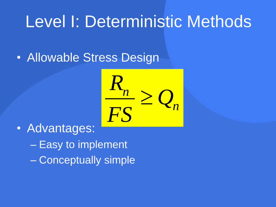
Level I: Deterministic Methods
• Allowable Stress Design
• Advantages:
– Easy to implement
– Conceptually simple
nn
RQ
FS

Level II: Semi-probabilistic Methods
• Load and Resistance Factor Design (LRFD)
η:load modifier; γ: load factor; ϕ: resistance factor
• Advantages:
– Consider uncertainties of R and Q
– A consistent format as ASD
i i i i iQ R

resistance factors
AASHTO LRFD Bridge Design Specifications
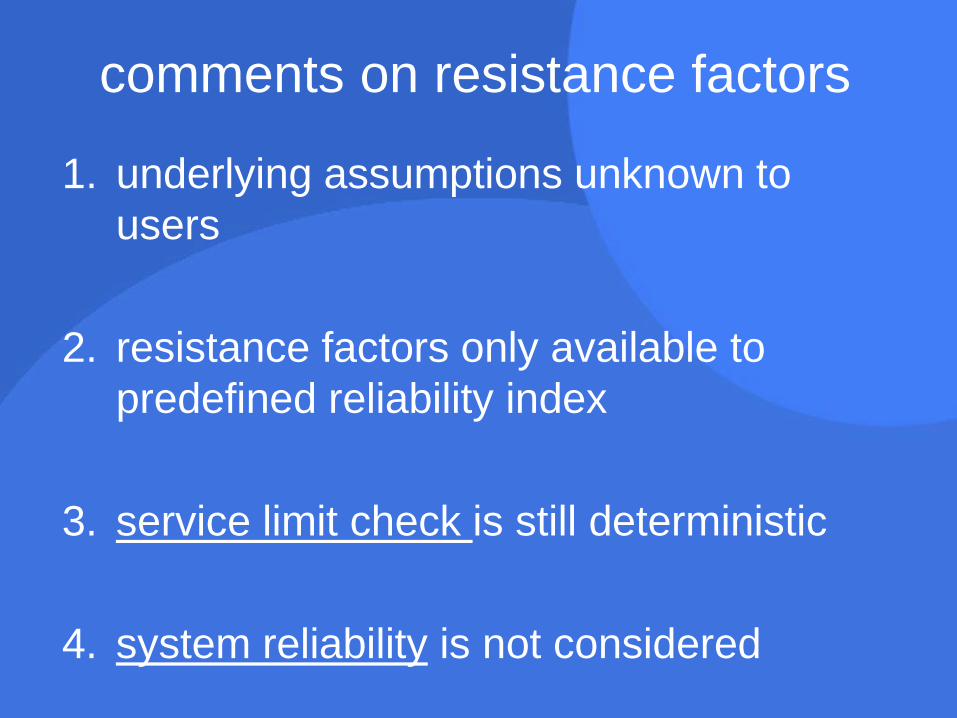
comments on resistance factors
1. underlying assumptions unknown to
users
2. resistance factors only available to
predefined reliability index
3. service limit check is still deterministic
4. system reliability is not considered
LRFD
implementation issue
Example
Axially Loaded Piles

• Ultimate capacity
• LRFD requires that
1 1 2 2 3 3R R R Q
1 2 3uR R R R
Q
R1
R2
R3
uR Q
or

The soil stratifications change!
Q Q Q
R1
R2
R3
1 2 3uR R R R

The soil stratifications change!
Ru
Ru
1 2 3uR R R R

Q V M
Q V M
Q V M
laterally loaded piles

observations
1. Soil stratifications differ from site to site.
2. The mean and/or variance of each soil
stratification would differ from site to site.
3. The same resistance factor is applied in
LRFD, regardless of soil stratifications.

CONCLUSION
A uniform level of safety cannot be
achieved in the LRFD framework,
when LRFD is implemented
independently of soil stratifications.
Reference
Ching, J.Y., Phoon, K.K., Chen, J.R. and Park, J.H.
(2013). “Robustness of constant load and resistance
factor design factors for drilled shafts in multiple strata.”
Journal of Geotechnical and Geoenvironmental
Engineering, Vol. 139(7):1104-1114.

PROBLEM STATEMENT
How to accommodate the
uncertainties in deep foundation
design?

an alternative to LRFD
in
reliability based design
computer-based reliability tools

Reliability-Based Design
• How to define the failure event ?
– design criteria
• How to calculate the failure probability?
– reliability analysis

Performance Based Design
(PBD) • design criteria
displacements
• parameter variability
random variable modeling
random field modeling for soil properties
mean, variance and correlation function
• Monte Carlo statistical methods
regular MCS
importance sampling

research methods

design criteria
• axial movement
• lateral deflection
• angular distortion

dep
th
soil property
random field
Q
sectional
stiffness, EA
•••
•••
toe spring
zn
tn
z2
t2
z1
t1
zn-1
tn-1
•••
w
q
side springs
t-z model

M V
Q
yn
pn
y2
p2
y1
p1
yn-1
pn-1
dep
th
soil property
random field
p-y method

design criteria in PBD
0 500 1000 15000
20
40
60
80
100
120
Sett
lem
en
t, m
m
Load, KN

random field
• distribution type
• mean
• variance
• correlation function
random
variable

correlation function
• To describe how points are correlated
spatially, a correlation function is required.
2
, exp

realizations of 1-D random fields -4
-2
0
2
4X
(z)
= 0.1
0 0.2 0.4 0.6 0.8 1-4
-2
0
2
4
z
X(z
)
= 4
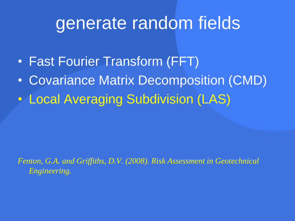
generate random fields
• Fast Fourier Transform (FFT)
• Covariance Matrix Decomposition (CMD)
• Local Averaging Subdivision (LAS)
Fenton, G.A. and Griffiths, D.V. (2008). Risk Assessment in Geotechnical
Engineering.

model errors
• load transfer curves
– p-y curves
– t-z curves
– q-w curves
• modeling of pile material
– concrete behavior
– steel behavior

accounting for model error
• The prediction most of the time deviates
from the measurement.
m pY e Y
Ym: The measurement
Yp: The prediction by using a model
e: Bias Factor, A Random Number that is applied to correct the
prediction
e may be a normal or lognormal variate.
In this study, N is assumed to be lognormal.

multiple failure modes
• structural failures
– bending moment, m
– shear, v
– axial force (ignored)
• performance-related failures
– lateral deflection, δ
– vertical movement, w
– angular distortion, α

system reliability
• structural failure
• performance-related failure
• system failure
struct M VP F P F F
perf wP F P F F F
system struct perfP F P F F

Tools: Computer Codes
1. Laterally loaded piles
2. Axially loaded piles
3. XPILE

inputs to computer codes
1. variability model of soil properties (µ,σ,θ)
2. variability model of concrete and steel
properties (probability distribution, µ,σ)
3. variability model of allowable
displacements
4. variability model of external loads
– live load component
– dead load component
5. uncertainty of load transfer curves

reliability analysis
• first order reliability method
• Monte Carlo simulation (MCS)

Deficiency of FORM
• For concave g(x’)
• For convex g(x’)
• For linear g(x’)
fP
fP
fP
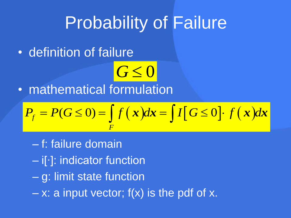
Probability of Failure
• definition of failure
• mathematical formulation
– f: failure domain
– i[∙]: indicator function
– g: limit state function
– x: a input vector; f(x) is the pdf of x.
( 0) 0f
F
P P G f d I G f d x x x x
0G

0 2 4 6 8 10
x 104
0
0.5
1
1.5
2
2.5
3x 10
-3
Number of samples
Pro
ba
bil
ity
of
fail
ure
1
1Failure
n
f i
i
P In

comments on MCS
• Mathematically simple to evaluate Pf
• Unbiased estimate of Pf
• But computationally demanding

• Limit state function
• X1 ~ standard normal variable
• X2 ~ standard normal variable
• Calculate P (G ≤ 0) using MCS
example of MCS
1 2 1 2, 3 2 12G x x x x

• Limit state function
• Reliability index
• Design point
FORM Solution
2 2
123.3282
3 2
1 2 1 2, 3 2 12G x x x x
* 2.7692,1.8462x
1 4.3704E 04fP

when you use
Monte Carlo simulations…
-6
-4
-2
0
2
4
6
-6 -1 4
Failure Domain
G < 0
Safe Domain
G >0
Limit State
G = 0
x2
x1
1
1Failure
n
f i
i
P In

observation
The crude MCS method has
low computational efficiency.

• Draw samples from a different function
• Importance Sampling Quotient
implement importance Sampling
0f
fP I G h d
h
xx x
x
1
10
n
IS i
i
fP I G
n h
x
x
fR
h
x
x

• crude MCS
• importance sampling
difference between mcs and is
,
1
10
n
f MCS i
i
P I Gn
,
1
10
n
f IS i
i
fP I G
n h
x
x

when you implement importance sampling method,
you will get…
-6
-4
-2
0
2
4
6
-6 -1 4
Failure Region
G < 0 Safe Region
G >0
Limit State
G = 0
x2
x1
Importance Sampling

0 200 400 600 800 10000
1
2
3
4
5
6
7
8
x 10-4
Number of Samples
Pro
bab
ilit
y o
f F
ailu
re
Importance SamplingP
IS = 4.4617E-04
COV = 6.17%n = 1000
Exact Solution

soil variability model
how to determine
μ, σ and θ

How to determine the variability
model of soil properties
• Standard penetration test (SPT) data is
used
• Bayesian approach
• Markov Chain Monte Carlo

Standard Penetration Test
Corrected N value
ER: Energy efficiency
N0
N1
N2
60 1 260
ERN N N
1 2N N N

Empirical correlations
• To convert SPT data to soil properties
0.72
600.29u aS N p
1 60
0
tan
12.2 20.3a
N
p
reference
Braja Das. Principles of Foundation Engineering, seventh edition. page 84 & 88.

Assumptions
1. Each N value is considered a unit in
Bayesian approach;
2. The mean, standard deviation and
correlation length do NOT change in the
unit;
3. Soil properties are lognormally
distributed.

Bayesian Approach
1. λ = (µ,σ,θ) are the parameters of interest;
X : log ( soil properties );
c : normalizing constant
2. L(λ|X) : Likelihood function
3. f′(λ) and f″ (λ) are prior and posterior PDF.
|f c L f X

observational data X
• Invoke Assumption #1.
0.72
600.29u aS N p
1 60
0
tan
12.2 20.3a
N
p
60 2 , 1,260
i
ERN N i
N0
N1
N2

likelihood function L
• Invoke Assumption #2 and #3
2 22
1 1| exp
2 12 1
TL
X X R X
1
1
R
ρ: correlation coefficient

Flow Chart

Example 1: Lateral Loading
Resource: Brown, D. A., Turner, J. P. and Casetelli, R. J. (2010). “Drilled shaft:
construction procedures and LRFD design methods.” No. FHWA-NHI-10-016, Federal
Highway Administration. page 12-27
Service load: H=111.2 kN (25 kips) and M=677.9 kN∙m (500 kip-ft.)

original design outcome
• shear = 25 kips and moment = 500 kip-ft
• D = 1.22 m (4 ft) and L = 6.10 m (20 ft)
• reinforced by 12 #11 bars with cover of 3
in.

parametric study
parameter probability
distribution mean cov θ
Su lognormal 103.4 KPa 40% varied
ε50 lognormal 0.005 20% varied
γ' lognormal 19.0 KN/m3 4% varied
conversion
Su: 103.4 Kpa = 15 psi
UW: 19 KN/m3 = 0.07 pci

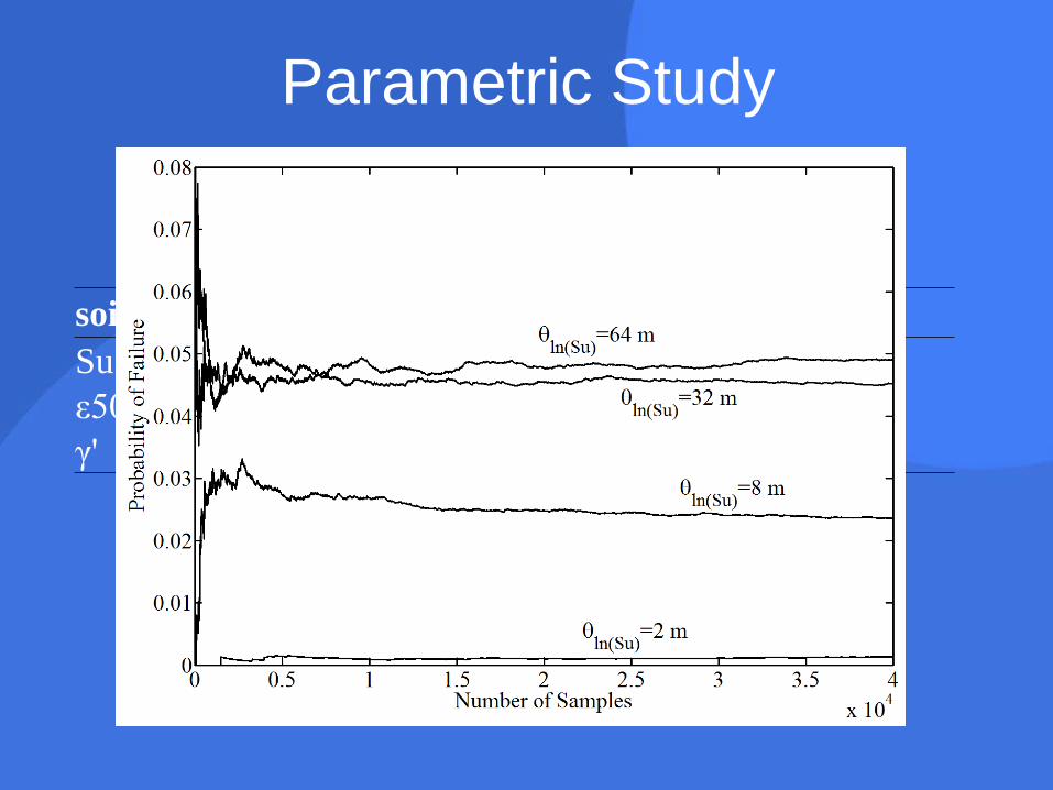
Parametric study
soil mean cov θ
Su 103.4 KPa 40% varied
ε50 0.005 20% 1.0 m
γ' 19.0 KN/m3 4% 1.0 m

Parametric study
soil mean cov θ
Su 103.4 KPa 40% varied
ε50 0.005 20% 1.0 m
γ' 19.0 KN/m3 4% 1.0 m

Parametric Study
soil properties mean cov θ
Su 103.4 kpa 40% varied
ε50 0.005 20% 1.0 m
γ' 19.0 kn/m3 4% 1.0 m
Parametric Study
soil properties mean cov θ
Su 103.4 kpa 40% varied
ε50 0.005 20% 1.0 m
γ' 19.0 kn/m3 4% 1.0 m

Effects of Spatial Variability of Su

-4
-2
0
2
4
X(z
)
= 0.1
0 0.2 0.4 0.6 0.8 1-4
-2
0
2
4
z
X(z
)
= 4

Example 2
importance sampling

parameters
• axial load = 1300 KN
• allowable settlement = 25 mm
• D = 1.10 m and L = 8.0 m
• soil type: clay
– average Su = 100 KPa, lognormal distributed
– COV = 20%
– correlation length θ = 1 m

crude Monte Carlo simulation
0 0.5 1 1.5 2 2.5 3
x 105
0
0.5
1
1.5
2
2.5
3x 10
-3
Number of Samples
Pro
ba
bil
ity
of
Fa
ilu
re
Regular MCSp
f = 0.0013
COV = 5.24%
= 3.022
Crude MCSP
f,MCS = 0.0013
COV = 5.24%
= 3.022

importance sampling
don’t wow…
0 200 400 600 800 10000
0.5
1
1.5
2
2.5
3x 10
-3
Number of Samples
Pro
ba
bil
ity
of
Fa
ilu
re
Importance samplingP
f,IS = 0.0012
COV = 6.13%
= 3.035
FORMP
f,FORM = 0.0016
= 2.939

Example 3
real-world project

outlines of the example
1. general description
2. use of markov chain monte carlo to
determine (µ,σ,θ)
3. use of kriging to estimate unknown
parameters
4. reliability analysis and design


subsurface investigation
2 to 12 inches of topsoil
8.5 to 26.5 ft of hard gray silt and clay
10.5 to 14.3 ft of silt and clay
15.5 ft of very stiff to hard brown and gray clay
18 to 30 ft of very stiff to hard clay, silty clay and silt
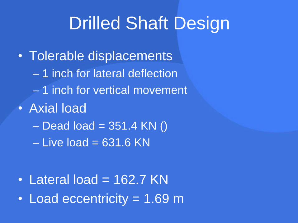
Drilled Shaft Design
• Tolerable displacements
– 1 inch for lateral deflection
– 1 inch for vertical movement
• Axial load
– Dead load = 351.4 KN ()
– Live load = 631.6 KN
• Lateral load = 162.7 KN
• Load eccentricity = 1.69 m
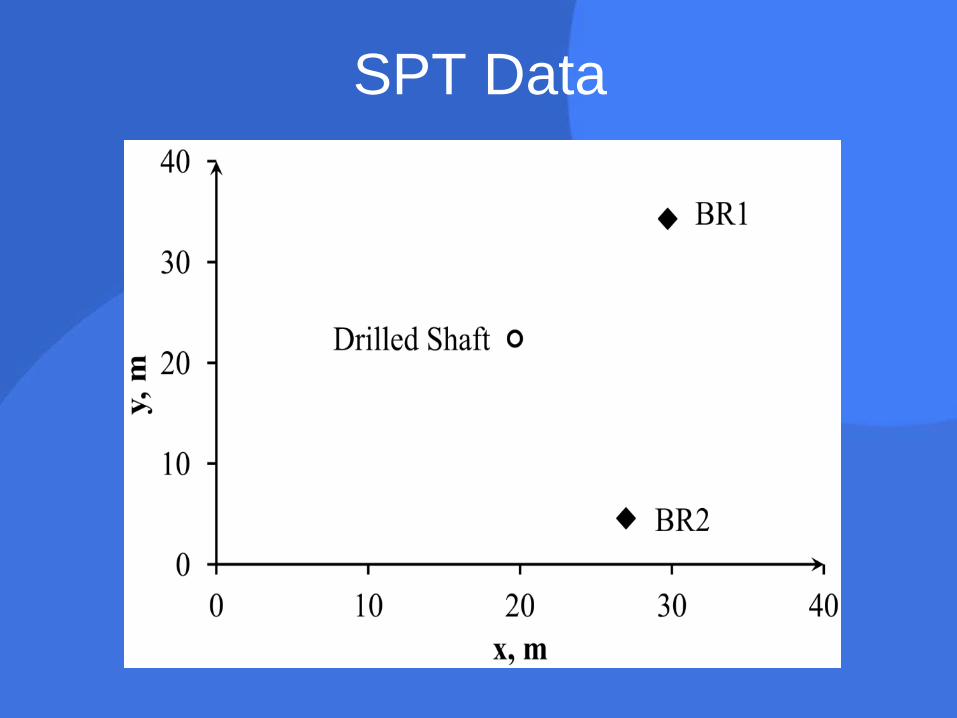
SPT Data

SPT Data

MCMC

MCMC
3
4
5
6
0
0.2
0.4
0.6
0 1000 2000 3000 4000 5000 6000 7000 8000 9000 100000
0.5
1
No. of Iterations

Statistical Analysis

Partial Results
Elevation
(m)
x
Soil
Strength
μ σ ρ θ (m) μx σx
256.5 ϕ′ 39.987 3.688 0.111 0.536 0.489 40.222 4.473
255.8 Su 218.740 5.360 0.285 0.392 0.326 221.55 64.375
255.0 Su 276.494 5.605 0.233 0.359 0.298 279.32 65.931
257.4 Su 93.621 4.549 0.502 0.663 0.742 107.20 57.353

correlation length θ
0.2 0.3 0.4 0.5 0.6 0.7 0.8 0.90
0.2
0.4
0.6
0.8
1
Cohesive SoilsSample Size = 18Minimum = 0.288 mMaximum = 0.751 mMean = 0.448 mStandard Deviation = 0.149 m
, m
Cu
mu
lati
ve
Dis
trib
uti
on
Fu
nct
ion
0.4 0.5 0.6 0.7 0.80
0.2
0.4
0.6
0.8
1
Granular SoilsSample Size = 27Minimum = 0.312 mMaximum = 0.771 mMean = 0.516 mStandard Deviation = 0.130 m
, m
Cu
mu
lati
ve D
istr
ibu
tio
n F
un
cti
on


Kriging
Tj is an observation and lj is the corresponding
distance between Tj and the interested location.
0
1
m
j j
j
T w T
1
, 1,2, ,m
v v
j j i
i
w l l j m
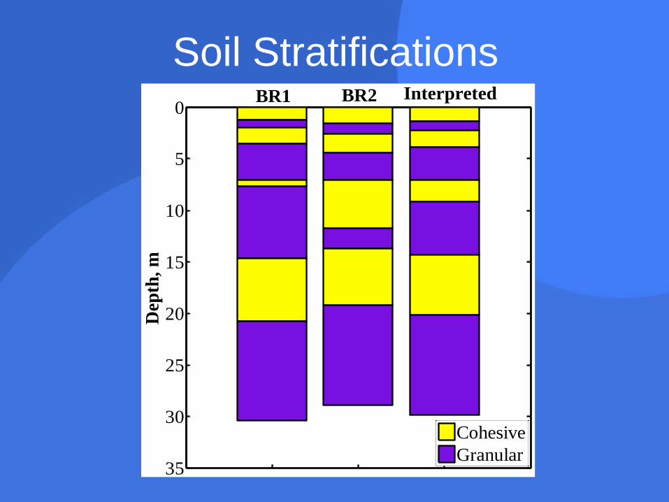
Soil Stratifications 0
5
10
15
20
25
30
35
Dep
th,
m
BR1 BR2 Interpreted
Cohesive
Granular

Interpreted Soil Profile
Elevation(m) x μx
253.0 ϕ′ 36.2
251.0 ϕ′ 36.2
251.0 Su 199.5
250.5 Su 199.4
250.0 Su 199.2
248.9 Su 199.0
248.9 ϕ′ 35.8

Interpreted soil profile
Soil Layer
BR1 BR2 Interpreted
σx θ (m) σx θ (m) σx θ (m)
#1 57.35 0.74 53.73 0.75 56.01 0.75
#2 4.47 0.49 4.49 0.51 4.48 0.50
#3 65.15 0.31 56.35 0.52 61.90 0.39
#4 4.38 0.56 4.27 0.58 4.34 0.57
#5 59.63 0.46 60.09 0.43 59.80 0.45
#6 4.58 0.46 4.55 0.46 4.57 0.46
#7 60.19 0.43 62.10 0.36 60.90 0.41
#8 4.65 0.45 4.60 0.45 4.63 0.45

Reliability Analysis Variable Distribution Mean COV Remarks
f'c Lognormal 31 MPa 7% ACI (2002)
fy Lognormal 415 MPa 5% Mirza and MacGregor (1979)
Es Lognormal 200 GPa 5% Mirza and MacGregor (1979)
epy Lognormal 1 10% (Assumed)
etz Lognormal 1 10% (Assumed)
eqw Lognormal 1 10% (Assumed)
da,δ Lognormal 2.54 cm 10% Zhang and Ng (2005)
da,w Lognormal 2.54 cm 10% Zhang and Ng (2005)
da,ψ — — — —
VD Lognormal 162.72 KN 25% Nowak and Collins (2000)
VL — — — —
QD Lognormal 351.39 KN 10% Nowak and Collins (2000)
QL Lognormal 631.62 KN 50% Nowak and Collins (2000)

old design
1. Diameter = 42 in.
2. Length = 83 ft.
3. Reinforcement: 20 #11 bars, cover
thickness = 3 in.

reliability analysis of original design
0 2 4 6 8 10
x 104
0
1
2
3
4
5
6x 10
-3
Number of Simulations
Pro
ba
bil
ity
of
Fa
ilu
re
Pf = 0.0028
Pf,
= 0.0028
Pf,w
= 0

new design
design parameters old design
diameter 42 in
length 83 ft
rebar 20 #11 bars
cover thickness 3 in
new design
42 in
55 ft
22 #11 bars
3 in

reliability analysis of new design
0 2 4 6 8 10
x 104
0
0.5
1
1.5x 10
-3
Number of Simulations
Pro
ba
bil
ity
of
Fa
ilu
re
Pf = 5.1E-4
Pf,
= 7.0E-5
Pf,w
= 4.4E-4
Target

factor of safety
• Old design: 5.215
• New design: 3.311

computer program XPILE

computer program XPILE

computer program XPILE

computer program XPILE

computer program XPILE

computer program XPILE

computer program XPILE

computer program XPILE

computer program XPILE

Summary and Conclusions
1. Performance-Based Design (PBD) is
developed for deep foundation design.
2. Soil properties are modeled as random
fields.
3. Probability of failure is sensitive to θ.
4. A few computer codes were developed.
5. System reliability should be considered if
multiple failure modes exist.

Recommendations for future research
• computer-based reliability tool for pile group;

Recommendations for future research
• statistics of tolerable displacements
dT: tolerable displacement
d: actual displacement
TG d d

Recommendations for future research
• to develop guidance of determining the
variability of external loads.
Q V M

Recommendations for future research
• to calibrate model errors
– p-y curves
– t-z curves and
– q-w curves

Thank you!