Performance Assessment and Enhancement of

Precision Controlled Structures During

Conceptual Design

Homero L. Gutierrez and David W. Miller

February 1999 SERC#1–99

This report is based on the unaltered thesis of Homero L. Gutierrez submitted to the

Department of Aeronautics and Astronautics in partial fulfillment of the requirements for

the degree of Doctor of Philosophy at the Massachusetts Institute of Technology.

2

Abstract

Future optical space systems such as interferometers and filled-aperture telescopes will ex-

tend the resolution and sensitivity offered by their on-orbit and ground-based predecessors.

These systems face the challenge of achieving nanometer and milli-arcsecond precision con-

trol of stellar light passing through the optical train of a lightweight, flexible structure

subjected to various disturbances. It is advantageous to assess the performance of initial

concepts of these precision systems early in the design stage to aid in the requirements

flowdown and resource allocation process. A complete end-to-end performance assessment

methodology is developed which incorporates disturbance, sensitivity, and uncertainty anal-

ysis tools within a common state-space framework. The disturbance analysis is conducted

using either a time-domain, frequency-domain, or Lyapunov approach to obtain nominal

predictions of performance metric root-mean-square (RMS) values. Calculating power spec-

tral density and cumulative RMS functions of the performance metrics allows critical system

modes and frequencies to be identified, and in some instances, contributions from each of the

disturbances can be determined. A Lagrange multiplier method is used to derive a governing

equation for the sensitivities of the performance metrics with respect to model parameters.

For a system whose structural dynamic equations are represented in modal form, the sensi-

tivities can be calculated exactly and efficiently with respect to modal frequencies, masses,

and damping ratios. The most critical modal parameters are carried into a parametric

uncertainty analysis that seeks to identify the worst-case performance RMS values. A con-

strained optimization technique is described which searches for the worst-case performance

over all allowable parameter values. When required, a performance enhancement approach

is used to apply controlled structures technologies such as input/output isolation to achieve

large performance changes. Structural modifications based on insight provided by a physi-

cal parameter sensitivity analysis are then employed to “fine tune” the performance to keep

the worst-case values within the requirements. Analytical physical parameter sensitivities

are experimentally validated on a truss structure and used to implement stiffness and mass

perturbations that reduce the tip displacement of a flexible appendage. The overall frame-

work is applied to an integrated model of the Space Interferometry Mission to demonstrate

its practical use on a large order system.

3

4

Acknowledgments

The author was supported by a National Defense Science and Engineering Graduate Fel-

lowship. The work was performed for the Jet Propulsion Laboratory under JPL Contract

#961123 (Modeling and Optimization of Dynamics and Control for the NASA Space Inter-

ferometry Mission and the Micro-Precision Interferometer Testbed), with Dr. Robert Laskin

as Technical/Scientific Officer, Dr. Sanjay Joshi as Contract Monitor, and Ms. SharonLeah

Brown as MIT Fiscal Officer.

5

6

Contents

1 Introduction 211.1 Background . . . . . . . . . . . . . . . . . . . . . . . . . . . . . . . . . . . . 211.2 Research Objectives and Approach . . . . . . . . . . . . . . . . . . . . . . . 231.3 Literature Review . . . . . . . . . . . . . . . . . . . . . . . . . . . . . . . . 241.4 Thesis Overview . . . . . . . . . . . . . . . . . . . . . . . . . . . . . . . . . 29

2 Integrated Modeling 312.1 Integrated Modeling Description . . . . . . . . . . . . . . . . . . . . . . . . 31

2.1.1 Motivation . . . . . . . . . . . . . . . . . . . . . . . . . . . . . . . . 312.1.2 Structural modeling . . . . . . . . . . . . . . . . . . . . . . . . . . . 332.1.3 Control modeling . . . . . . . . . . . . . . . . . . . . . . . . . . . . . 352.1.4 Performance modeling . . . . . . . . . . . . . . . . . . . . . . . . . . 372.1.5 Disturbance modeling . . . . . . . . . . . . . . . . . . . . . . . . . . 392.1.6 Numerical conditioning . . . . . . . . . . . . . . . . . . . . . . . . . 44

2.2 Space Interferometry Mission Overview . . . . . . . . . . . . . . . . . . . . 462.2.1 Modes of operation . . . . . . . . . . . . . . . . . . . . . . . . . . . . 482.2.2 Finite-element model . . . . . . . . . . . . . . . . . . . . . . . . . . . 512.2.3 Optical model . . . . . . . . . . . . . . . . . . . . . . . . . . . . . . . 542.2.4 Optical control . . . . . . . . . . . . . . . . . . . . . . . . . . . . . . 562.2.5 Reaction wheel assembly stochastic disturbance model . . . . . . . . 60

2.3 Summary . . . . . . . . . . . . . . . . . . . . . . . . . . . . . . . . . . . . . 75

3 Disturbance Analysis Framework 773.1 Types of Disturbance Analyses . . . . . . . . . . . . . . . . . . . . . . . . . 77

3.1.1 Time-domain analysis . . . . . . . . . . . . . . . . . . . . . . . . . . 783.1.2 Frequency-domain analysis . . . . . . . . . . . . . . . . . . . . . . . 793.1.3 Lyapunov analysis . . . . . . . . . . . . . . . . . . . . . . . . . . . . 843.1.4 Comments . . . . . . . . . . . . . . . . . . . . . . . . . . . . . . . . . 87

3.2 Demonstration of Analysis Methods on a Single DOF System . . . . . . . . 873.3 Frequency-Domain Disturbance Analysis on SIM . . . . . . . . . . . . . . . 923.4 Summary . . . . . . . . . . . . . . . . . . . . . . . . . . . . . . . . . . . . . 102

4 Sensitivity Analysis Framework 1034.1 System State-Space Representation . . . . . . . . . . . . . . . . . . . . . . . 1044.2 Governing Sensitivity Equation . . . . . . . . . . . . . . . . . . . . . . . . . 1064.3 Modal Parameter Sensitivities . . . . . . . . . . . . . . . . . . . . . . . . . . 108

4.3.1 Structural modal form . . . . . . . . . . . . . . . . . . . . . . . . . . 108

7

4.3.2 Simplification of governing equation . . . . . . . . . . . . . . . . . . 1114.4 Demonstration of Modal Parameter Sensitivity Analysis . . . . . . . . . . . 113

4.4.1 Single DOF system . . . . . . . . . . . . . . . . . . . . . . . . . . . . 1144.4.2 Multi-DOF system . . . . . . . . . . . . . . . . . . . . . . . . . . . . 1164.4.3 SIM Classic . . . . . . . . . . . . . . . . . . . . . . . . . . . . . . . . 117

4.5 Physical Parameter Sensitivities . . . . . . . . . . . . . . . . . . . . . . . . . 1254.5.1 Derivation of physical parameter sensitivities . . . . . . . . . . . . . 1264.5.2 Mode shape and natural frequency derivatives . . . . . . . . . . . . . 1304.5.3 Implementation . . . . . . . . . . . . . . . . . . . . . . . . . . . . . . 137

4.6 Demonstration of Physical Parameter Sensitivity Analysis . . . . . . . . . . 1404.6.1 Cantilever beam . . . . . . . . . . . . . . . . . . . . . . . . . . . . . 1404.6.2 SIM Classic . . . . . . . . . . . . . . . . . . . . . . . . . . . . . . . . 147

4.7 MATLAB Implementation . . . . . . . . . . . . . . . . . . . . . . . . . . . . 1544.8 Summary . . . . . . . . . . . . . . . . . . . . . . . . . . . . . . . . . . . . . 155

5 Uncertainty Analysis Framework 1575.1 Types of model uncertainties . . . . . . . . . . . . . . . . . . . . . . . . . . 1585.2 Parametric Uncertainty Analysis Methods . . . . . . . . . . . . . . . . . . . 159

5.2.1 Evaluation of “bad corners” . . . . . . . . . . . . . . . . . . . . . . . 1605.2.2 First-order approach . . . . . . . . . . . . . . . . . . . . . . . . . . . 1615.2.3 Constrained optimization approach . . . . . . . . . . . . . . . . . . . 1635.2.4 Robust control approach . . . . . . . . . . . . . . . . . . . . . . . . . 164

5.3 Approximate Performance and Sensitivity Calculations . . . . . . . . . . . . 1685.3.1 Balanced model reduction . . . . . . . . . . . . . . . . . . . . . . . . 1695.3.2 Analysis approximations during optimization iterations . . . . . . . 173

5.4 Demonstration of Uncertainty Analysis . . . . . . . . . . . . . . . . . . . . . 1775.4.1 Single DOF system . . . . . . . . . . . . . . . . . . . . . . . . . . . . 1775.4.2 Cantilever beam . . . . . . . . . . . . . . . . . . . . . . . . . . . . . 1815.4.3 Multi-DOF system . . . . . . . . . . . . . . . . . . . . . . . . . . . . 1885.4.4 SIM Classic . . . . . . . . . . . . . . . . . . . . . . . . . . . . . . . . 196

5.5 Summary . . . . . . . . . . . . . . . . . . . . . . . . . . . . . . . . . . . . . 200

6 Experimental Validation 2036.1 Description of Testbed . . . . . . . . . . . . . . . . . . . . . . . . . . . . . . 2046.2 Testbed Model . . . . . . . . . . . . . . . . . . . . . . . . . . . . . . . . . . 2106.3 Automated Finite-Element Model Updating . . . . . . . . . . . . . . . . . . 2126.4 Disturbance Analysis Results . . . . . . . . . . . . . . . . . . . . . . . . . . 2186.5 Sensitivity Analysis Results . . . . . . . . . . . . . . . . . . . . . . . . . . . 2196.6 Performance Enhancement Exercise . . . . . . . . . . . . . . . . . . . . . . 2306.7 Summary . . . . . . . . . . . . . . . . . . . . . . . . . . . . . . . . . . . . . 234

7 Performance Enhancement Framework 2357.1 Methodology . . . . . . . . . . . . . . . . . . . . . . . . . . . . . . . . . . . 2357.2 Application to SIM Classic . . . . . . . . . . . . . . . . . . . . . . . . . . . 2377.3 Summary . . . . . . . . . . . . . . . . . . . . . . . . . . . . . . . . . . . . . 256

8

8 Conclusions and Recommendations 2598.1 Thesis Summary . . . . . . . . . . . . . . . . . . . . . . . . . . . . . . . . . 2598.2 Contributions . . . . . . . . . . . . . . . . . . . . . . . . . . . . . . . . . . . 2668.3 Recommendations for Future Work . . . . . . . . . . . . . . . . . . . . . . . 268

A Performance Assessment and Enhancement of NGST 273

B Derivation of RWA Disturbance Cross-Spectral Density Function 295

C Derivation of Curvature Equation 297

References 301

9

10

List of Figures

1.1 Performance assessment and enhancement framework. . . . . . . . . . . . . 221.2 Analysis procedure. . . . . . . . . . . . . . . . . . . . . . . . . . . . . . . . . 30

2.1 Open-loop system provided by structural modeling. . . . . . . . . . . . . . . 342.2 Additions made by control modeling. . . . . . . . . . . . . . . . . . . . . . . 362.3 Addition made by performance modeling. . . . . . . . . . . . . . . . . . . . 372.4 Addition made by disturbance modeling. . . . . . . . . . . . . . . . . . . . . 392.5 Timeline of Origins Program missions . . . . . . . . . . . . . . . . . . . . . 472.6 SIM Classic concept . . . . . . . . . . . . . . . . . . . . . . . . . . . . . . . 472.7 Schematic of the basic elements of an interferometer. . . . . . . . . . . . . . 492.8 (a) Flat mirror attached to a gimbal [4]. (b) Fast-steering mirror [3]. . . . . 502.9 (a) SIM finite-element model. (b) Ray trace through +x arm of guide #1

interferometer. . . . . . . . . . . . . . . . . . . . . . . . . . . . . . . . . . . 522.10 (a) Bottom view of ray trace. (b) Side view of ray trace. (c) Bottom view of

ray trace through siderostat bay. (d) Side view of ray trace through siderostatbay. . . . . . . . . . . . . . . . . . . . . . . . . . . . . . . . . . . . . . . . . 55

2.11 Side view of ray trace through ODL assembly. . . . . . . . . . . . . . . . . . 562.12 (a) Block diagram of ODL and fringe tracker controllers. (b) Block diagram

of ACS controller. . . . . . . . . . . . . . . . . . . . . . . . . . . . . . . . . 572.13 (a) Transfer function magnitudes of voice coil controller Kvc (top) and PZT

controller Kpzt (bottom). (b) Transfer function magnitudes of fringe trackercontroller. . . . . . . . . . . . . . . . . . . . . . . . . . . . . . . . . . . . . . 59

2.14 (a) Singular values of ODL sensitivity transfer function matrix. (b) Singularvalues of fringe tracker sensitivity transfer function matrix (with internalmetrology loop closed). . . . . . . . . . . . . . . . . . . . . . . . . . . . . . . 60

2.15 (a) ACS compensator. (b) Singular values of ACS sensitivity transfer func-tion matrix. . . . . . . . . . . . . . . . . . . . . . . . . . . . . . . . . . . . . 61

2.16 Local wheel frame . . . . . . . . . . . . . . . . . . . . . . . . . . . . . . . . 642.17 XY Z Euler angles . . . . . . . . . . . . . . . . . . . . . . . . . . . . . . . . 652.18 Position vector r, which locates the wheel frame origin in the spacecraft frame 662.19 Power spectral density functions of disturbances from a Hubble-class reaction

wheel . . . . . . . . . . . . . . . . . . . . . . . . . . . . . . . . . . . . . . . 732.20 Power spectral density functions of disturbances in spacecraft frame . . . . 742.21 Representative cross-spectral density functions of disturbances in spacecraft

frame . . . . . . . . . . . . . . . . . . . . . . . . . . . . . . . . . . . . . . . 74

3.1 Plant disturbance-to-performance filter. . . . . . . . . . . . . . . . . . . . . 783.2 Disturbance filter and plant disturbance-to-performance filter. . . . . . . . . 80

11

3.3 White noise-to-performance filter. . . . . . . . . . . . . . . . . . . . . . . . . 853.4 Single DOF system. . . . . . . . . . . . . . . . . . . . . . . . . . . . . . . . 883.5 (a) Disturbance PSD and cumulative RMS. (b) Disturbance time history. . 883.6 (a) Performance PSD and cumulative RMS curve computed from the time

history shown in (b). . . . . . . . . . . . . . . . . . . . . . . . . . . . . . . . 893.7 Performance PSD (bottom) and cumulative RMS (top) from frequency-domain

analysis. . . . . . . . . . . . . . . . . . . . . . . . . . . . . . . . . . . . . . . 903.8 Effects of (a) frequency resolution and (b) truncated time-domain simulation. 913.9 Stellar ray trace through guide interferometer #1 of SIM. . . . . . . . . . . 933.10 Example of balanced model reduction on original system (plots on left) and

system with scaled output 2 (plots on right). . . . . . . . . . . . . . . . . . 953.11 Example disturbance-to-performance transfer function before and after model

is reduced. . . . . . . . . . . . . . . . . . . . . . . . . . . . . . . . . . . . . . 963.12 Cumulative RMS curves (top) and PSD’s (bottom) of RWA disturbances. . 973.13 RMS estimates of the five performance metrics as a function of frequency

resolution, model order, and disturbance correlation. . . . . . . . . . . . . . 983.14 Computation times corresponding to the runs in Figure 3.13. . . . . . . . . 993.15 Cumulative RMS (top), PSD (middle), and disturbance contribution (bot-

tom) for total OPD. . . . . . . . . . . . . . . . . . . . . . . . . . . . . . . . 1003.16 Cumulative variance plot used to identify critical frequencies. . . . . . . . . 1013.17 Bar chart showing percent contribution of each mode to overall performance

variance. Disturbance contribution to PSD at each frequency is indicated bythe relative partition of each bar. . . . . . . . . . . . . . . . . . . . . . . . . 101

4.1 Disturbance filter and plant disturbance-to-performance filter. . . . . . . . . 1044.2 (a) Single DOF system. (b) Disturbance PSD (bottom) and cumulative RMS

(top). . . . . . . . . . . . . . . . . . . . . . . . . . . . . . . . . . . . . . . . 1144.3 Normalized sensitivities of SDOF system performance with respect to modal

parameters. . . . . . . . . . . . . . . . . . . . . . . . . . . . . . . . . . . . . 1154.4 Magnitudes of the percent errors in the finite-difference approximation to

the sensitivities with respect to frequency (left) and damping (right) as afunction of parameter perturbation size. . . . . . . . . . . . . . . . . . . . . 116

4.5 (a) 20 DOF spring/mass system. (b) Disturbance PSD’s (bottom) and cu-mulative RMS (top). (c) Performance PSD (bottom) and cumulative RMS(top). (d) Normalized sensitivities of critical modes. . . . . . . . . . . . . . 118

4.6 Magnitudes of the percent errors in the finite-difference approximation tothe sensitivities with respect to frequency (left) and damping (right) as afunction of parameter perturbation size. . . . . . . . . . . . . . . . . . . . . 119

4.7 Analytical RWA disturbance PSD’s and approximate PSD’s from low-orderfilter (bottom). Cumulative RMS curves (top). . . . . . . . . . . . . . . . . 122

4.8 (a) Approximate PSD’s from low-order filter, and cumulative RMS curves.(b) Performance PSD, cumulative RMS, and disturbance contribution. . . . 122

4.9 (a) Cumulative performance variance. (b) Critical frequencies and distur-bances. . . . . . . . . . . . . . . . . . . . . . . . . . . . . . . . . . . . . . . . 123

4.10 Normalized modal parameter sensitivities. . . . . . . . . . . . . . . . . . . . 1244.11 Magnitudes of the percent errors in the finite-difference approximation to

the sensitivities with respect to frequency (left) and damping (right) as afunction of perturbation size. . . . . . . . . . . . . . . . . . . . . . . . . . . 125

12

4.12 (a) Cantilever beam demonstration case. (b) Tip force disturbance PSD. (c)Tip displacement cumulative RMS (top) and PSD (bottom). . . . . . . . . 141

4.13 (a) Performance RMS normalized sensitivities with respect to modal param-eters. (b) Strain energy contributions to each mode from the four types ofbeam deformation. . . . . . . . . . . . . . . . . . . . . . . . . . . . . . . . . 142

4.14 Bar chart representation of Table 4.5. . . . . . . . . . . . . . . . . . . . . . 1464.15 (a) Stellar ray trace through guide interferometer #1 of SIM. (b) Approxi-

mate PSD’s (bottom) and cumulative RMS (top) of reaction wheel distur-bances. (c) Performance PSD (bottom) and cumulative RMS (top). (d)Normalized sensitivities of performance RMS with respect to modal param-eters of critical modes. . . . . . . . . . . . . . . . . . . . . . . . . . . . . . . 148

4.16 (a) Strain energy contributions for the 16.95 Hz mode. (b) Mode shape ofthe 16.95 Hz mode. . . . . . . . . . . . . . . . . . . . . . . . . . . . . . . . . 149

4.17 (a) Strain energy contributions for the 18.91 Hz mode. (b) Mode shape ofthe 18.91 Hz mode. (c) Strain energy contributions for the 21.39 Hz mode.(d) Mode shape of the 21.39 Hz mode. . . . . . . . . . . . . . . . . . . . . . 151

4.18 SIM physical parameter sensitivities. . . . . . . . . . . . . . . . . . . . . . . 153

5.1 Example uncertainty bounds for different designs. . . . . . . . . . . . . . . . 1585.2 Parameter space for the case of two uncertain parameters. . . . . . . . . . . 1605.3 Uncertain system modeled by ∆ block in feedback with nominal system. . . 1655.4 Model reduction options during constrained optimization uncertainty analy-

sis. (a) No model reduction. (b) Exact balanced reduction at each iteration.(c) Approximate balanced reduction at each iteration step. Both (b) and (c)rely on approximate cost and sensitivity evaluations. . . . . . . . . . . . . . 175

5.5 (a) Single DOF system. (b) Normalized sensitivities. (c) Disturbance PSD(bottom) and cumulative RMS (top). (d) Performance PSD (bottom) andcumulative RMS (top). . . . . . . . . . . . . . . . . . . . . . . . . . . . . . . 179

5.6 Results of uncertainty analysis on single DOF case. Bottom plot, parametervalues: Constrained optimization initial guess, , and converged solution, ∗.Parameter #1 = ωn, #2 = ζ, #3 = m. · · ·: upper or lower bound. Topplot, RMS values: −−− nominal; · · · initial guess; ∗−∗ worst case; −·−first-order approximation. . . . . . . . . . . . . . . . . . . . . . . . . . . . . 180

5.7 (a) Time statistics for constrained optimization uncertainty analysis. (b) Per-cent differences between first-order approach and constrained optimization asa function of uncertainty size. . . . . . . . . . . . . . . . . . . . . . . . . . . 181

5.8 Cantilevered beam with nearly square cross-section. . . . . . . . . . . . . . 1825.9 Tip displacement PSD’s and cumulative RMS curves for systems with various

combinations of first and second mode frequencies. (a) Full frequency range.(b) Zoom around first two modes. . . . . . . . . . . . . . . . . . . . . . . . . 183

5.10 (a) Normalized sensitivities for the first four modes. (b) Tip displacementPSD’s and cumulative RMS curves for system with frequencies placed atlower bounds (−) and for system with frequencies specified by uncertaintyanalysis results (−−). . . . . . . . . . . . . . . . . . . . . . . . . . . . . . . 183

5.11 Various plots obtained when ω1 (∗ − ∗) is swept up while ω2 (× − −×) isswept down. (a) Top: normalized sensitivity w.r.t. ω; bottom: performanceRMS. (b) Top: normalized sensitivity w.r.t. ζ; bottom: normalized sensitivityw.r.t. m. . . . . . . . . . . . . . . . . . . . . . . . . . . . . . . . . . . . . . . 184

13

5.12 Results of uncertainty analysis optimization after ten runs for beam withclosely-space modes. (a) Uncertainties only in frequencies of first two modes.(b) Uncertainties in frequency, damping, and modal mass of first two modes. 185

5.13 (a) Tip displacement PSD’s and cumulative RMS curves for systems withvarious combinations of first and second mode frequencies. (b) Normalizedsensitivities for the first four modes. . . . . . . . . . . . . . . . . . . . . . . 186

5.14 Various plots obtained when ω1 (∗ − −∗) is swept up while ω2 (× − ×) isswept down. (a) Top: normalized sensitivity w.r.t. ω; bottom: performanceRMS. (b) Top: normalized sensitivity w.r.t. ζ; bottom: normalized sensitivityw.r.t. m . . . . . . . . . . . . . . . . . . . . . . . . . . . . . . . . . . . . . . 187

5.15 Results of uncertainty analysis optimization after ten runs for beam with well-separated modes. (a) Uncertainties only in frequencies of first two modes.(b) Uncertainties in frequency, damping, and modal mass of first two modes. 187

5.16 (a) 20 DOF spring/mass system. (b) Disturbance PSD’s (bottom) and cu-mulative RMS (top). (c) Performance PSD (bottom) and cumulative RMS(top). (d) Normalized sensitivities of critical modes. . . . . . . . . . . . . . 189

5.17 Results of uncertainty analysis optimization after ten runs. (a) Full-ordermodel without gradient calculations. (b) Full-order model with gradientcalculations. . . . . . . . . . . . . . . . . . . . . . . . . . . . . . . . . . . . . 191

5.18 (a) Time statistics for different order models when gradients are or are notsupplied. ∗: 42 states, no gradient info., : 42 states, w/ gradient info., :28 states, w/ gradient info., 2: 28 states, no gradient info. (b) Effects ofuncertainty size on accuracy of first-order uncertainty analysis. . . . . . . . 192

5.19 (a) Performance PSD’s of different order models (bottom) and cumulativeRMS (top). (b) Gramian values of balanced full-order system. . . . . . . . . 192

5.20 (a) Time statistics for different order models (gradients are supplied in eachcase). (b) Percent errors between worst-case RMS predicted by reduced-ordermodels and worst-case RMS predicted by full-order model. . . . . . . . . . . 193

5.21 Results of uncertainty analysis optimization after ten runs. (a) Reduced-order model (28 states) without gradient calculations. (b) Reduced-ordermodel (28 states) with gradient calculations. . . . . . . . . . . . . . . . . . . 194

5.22 (a) Gramian values of exactly balanced system and approximately balancedsystem. Values shown are for one specific iteration during uncertainty op-timization run. (b) Average error in approximate sensitivity computationduring uncertainty optimization run. . . . . . . . . . . . . . . . . . . . . . . 195

5.23 (a) Stellar ray trace through guide interferometer #1 of SIM. (b) Approxi-mate PSD’s (bottom) and cumulative RMS (top) of reaction wheel distur-bances. (c) Performance PSD (bottom) and cumulative RMS (top). (d)Normalized sensitivities of performance RMS with respect to modal param-eters of critical modes. . . . . . . . . . . . . . . . . . . . . . . . . . . . . . . 197

5.24 (a) Uncertainty analysis runs when SIM model is reduced to 150 states ateach iteration. (b) Uncertainty analysis runs when SIM model is reducedto 120 states at each iteration. Both plots: , initial guess; ∗, convergedsolution; · · ·, upper or lower bound; − − −, nominal; 2, exact; − · −, first-order approximation. . . . . . . . . . . . . . . . . . . . . . . . . . . . . . . . 199

5.25 Gramian values of SIM model. . . . . . . . . . . . . . . . . . . . . . . . . . 2005.26 Uncertainty analysis runs when SIM model is reduced to 150 states at each

iteration. (nine uncertain parameters) . . . . . . . . . . . . . . . . . . . . . 201

14

6.1 (a) View of entire testbed. (b) Close-up of flexible appendage. (c) Compo-nents of flexible appendage. . . . . . . . . . . . . . . . . . . . . . . . . . . . 207

6.2 (a) Close-up of J-struts. (b) Close-up of stiff spring with added soft springs.(c) Close-up of shaker. . . . . . . . . . . . . . . . . . . . . . . . . . . . . . . 208

6.3 Four views of the testbed finite-element model. . . . . . . . . . . . . . . . . 2106.4 Comparison of transfer functions from data, updated FEM, and two types of

un-updated FEM . . . . . . . . . . . . . . . . . . . . . . . . . . . . . . . . . 2186.5 (a) Modal parameter sensitivities. (b) Measured load cell PSD. (c) Measured

(—) and predicted (−−) tip displacement PSD’s and cumulative RMS curves.2206.6 (a) Predicted and measured physical parameter sensitivities. (b) Predicted

and measured RMS values. . . . . . . . . . . . . . . . . . . . . . . . . . . . 2246.7 Comparison of measured (left column) and FEM (right column) PSD’s and

cumulative RMS curves. — Nominal (4 mil shim), −− 14 mil shim, − · − 2mil shim, · · · no shim. . . . . . . . . . . . . . . . . . . . . . . . . . . . . . . 228

6.8 Comparison of measured (left column) and FEM (right column) PSD’s andcumulative RMS curves. — Nominal (0 soft springs), −− 2 soft springs, −·−4 soft springs. . . . . . . . . . . . . . . . . . . . . . . . . . . . . . . . . . . . 229

6.9 Predicted physical parameter sensitivities based on different finite-elementmodels. . . . . . . . . . . . . . . . . . . . . . . . . . . . . . . . . . . . . . . 230

6.10 Weighted sensitivities. . . . . . . . . . . . . . . . . . . . . . . . . . . . . . . 2326.11 Comparison of measured (left column) and FEM (right column) PSD’s and

cumulative RMS curves. — Nominal , −− Redesign 1, − · − Redesign 2. . . 233

7.1 Controlled structures technology framework. . . . . . . . . . . . . . . . . . . 2377.2 SIM optical performance metrics as a function of isolator corner frequency

and levels of optical control. Structural damping = 0.1%. (Based on HSTRWA 0–3000 RPM disturbance model.) . . . . . . . . . . . . . . . . . . . . . 240

7.3 (a) Differential wavefront tilt of guide interferometer #1 with open opticsloops and either no isolation or a 10 Hz isolator. (b) Total OPD of guideinterferometer #1 with no isolation and either open or closed optics loops. . 241

7.4 Loop transfer function for one of twelve fast-steering mirror loops. . . . . . 2437.5 (a) Sample system to demonstrate washout effect. (b) Transfer function from

disturbance to differential tip displacement for various isolators. (b) Transferfunction from disturbance to differential tip rotation for various isolators. . 245

7.6 Disturbance PSD’s for the 0–3000 RPM case (—) and for the 0–600 RPMcase (−−). . . . . . . . . . . . . . . . . . . . . . . . . . . . . . . . . . . . . . 246

7.7 SIM optical performance metrics as a function of isolator corner frequencyand levels of optical control. Structural damping = 0.1%. (Based on HSTRWA 0–600 RPM disturbance model.) . . . . . . . . . . . . . . . . . . . . . 247

7.8 (a) Differential wavefront tilt of guide interferometer #1 with closed FSMloops and either a 0–3000 RPM RWA speed range or a 0-600 RPM speedrange (10 Hz isolator). (b) Total OPD of guide interferometer #1 with closedpathlength loops and either a 0–3000 RPM RWA speed range or a 0-600 RPMspeed range (5 Hz isolator). . . . . . . . . . . . . . . . . . . . . . . . . . . . 248

7.9 SIM optical performance metrics as a function of isolator corner frequencyand levels of optical control. Structural damping = 1%. (Based on HSTRWA 0–3000 RPM disturbance model.) . . . . . . . . . . . . . . . . . . . . . 250

15

7.10 (a) PSD, cumulative RMS, and disturbance contribution plots of weightedOPD for guide 1 and guide 2. (b) Critical modes and disturbances. (b)Modal parameter sensitivities of weighted OPD. . . . . . . . . . . . . . . . . 252

7.11 Physical parameter sensitivities. . . . . . . . . . . . . . . . . . . . . . . . . . 2537.12 PSD’s and cumulative RMS curves for the nominal design and the design

with 15% decrease in torsional constant J and 15% decrease in siderostatbay stiffnesses. . . . . . . . . . . . . . . . . . . . . . . . . . . . . . . . . . . 254

8.1 New SIM Concept. . . . . . . . . . . . . . . . . . . . . . . . . . . . . . . . . 271

A.1 Finite-element model of an early NGST concept. . . . . . . . . . . . . . . . 276A.2 Four modes of the finite-element model. . . . . . . . . . . . . . . . . . . . . 276A.3 Disturbance PSD’s. . . . . . . . . . . . . . . . . . . . . . . . . . . . . . . . . 277A.4 Ray trace used to define DPL and WFT. . . . . . . . . . . . . . . . . . . . 278A.5 DPL PSD’s. . . . . . . . . . . . . . . . . . . . . . . . . . . . . . . . . . . . . 281A.6 WFT PSD’s. . . . . . . . . . . . . . . . . . . . . . . . . . . . . . . . . . . . 282A.7 DPL as a function of location on mirror. . . . . . . . . . . . . . . . . . . . . 283A.8 WFT as a function of location on mirror. . . . . . . . . . . . . . . . . . . . 284A.9 Tower frequency trade study. . . . . . . . . . . . . . . . . . . . . . . . . . . 285A.10 Backsheet stiffness trade study. . . . . . . . . . . . . . . . . . . . . . . . . . 286A.11 Modal damping trade study. . . . . . . . . . . . . . . . . . . . . . . . . . . . 287A.12 Tower modal damping trade study. . . . . . . . . . . . . . . . . . . . . . . . 288A.13 Mirror modal damping trade study. . . . . . . . . . . . . . . . . . . . . . . . 289A.14 Isolator corner frequency trade study. . . . . . . . . . . . . . . . . . . . . . 289

16

List of Tables

2.1 Listing of some spacecraft disturbances. . . . . . . . . . . . . . . . . . . . . 402.2 Dependence of CCD integration time and fringe tracker bandwidth on stellar

magnitude . . . . . . . . . . . . . . . . . . . . . . . . . . . . . . . . . . . . . 58

4.1 Number of Lyapunov equations needed for exact and approximate sensitivitycalculations. ns is the number of states in Azd. . . . . . . . . . . . . . . . . 113

4.2 DOF ordering for a single, two-node Bernoulli-Euler beam element. . . . . . 1344.3 Cantilever beam frequencies and mode shapes. . . . . . . . . . . . . . . . . 1424.4 Notation used for the four types of beam deformation. (jth mode, kth beam

element) . . . . . . . . . . . . . . . . . . . . . . . . . . . . . . . . . . . . . . 1434.5 Comparison of tip displacement RMS normalized sensitivities with respect

to beam properties. . . . . . . . . . . . . . . . . . . . . . . . . . . . . . . . . 146

5.1 Uncertain parameters for single DOF case. . . . . . . . . . . . . . . . . . . . 1785.2 Uncertain parameters for multi-DOF case. . . . . . . . . . . . . . . . . . . . 1905.3 Uncertain parameters for SIM case. . . . . . . . . . . . . . . . . . . . . . . . 199

6.1 Desired characteristics of testbed. . . . . . . . . . . . . . . . . . . . . . . . . 2066.2 Testbed components. . . . . . . . . . . . . . . . . . . . . . . . . . . . . . . . 2096.3 Supporting experimental hardware. . . . . . . . . . . . . . . . . . . . . . . . 2096.4 Parameter values for un-updated and updated models. . . . . . . . . . . . . 2176.5 Sensitivity validation test matrix. . . . . . . . . . . . . . . . . . . . . . . . . 222

7.1 Application of CST options during performance enhancement process. . . . 2387.2 Comparison of RMS values for different SIM designs. . . . . . . . . . . . . . 2497.3 Comparison of RMS values for different SIM designs. . . . . . . . . . . . . . 255

A.1 Results of disturbance analysis on nominal NGST model. . . . . . . . . . . 280A.2 Comparison of use of controlled structures technologies. . . . . . . . . . . . 290A.3 Results of CST Layering. . . . . . . . . . . . . . . . . . . . . . . . . . . . . 292

C.1 Number of Lyapunov equations needed for exact sensitivity and curvaturecalculations. . . . . . . . . . . . . . . . . . . . . . . . . . . . . . . . . . . . . 299

17

18

Nomenclature

AbbreviationsACS attitude control systemCMG control moment gyroCST controlled structures technologiesDOF degree of freedomEVP eigenvalue problemFEM finite-element model; finite-element methodFSM fast steering mirrorIMOS Integrated Modeling of Optical SystemsJPL Jet Propulsion LaboratoryNGST Next Generation Space TelescopeODL optical delay lineOPD optical path differencePDF probability density functionPSD power spectral densityRBE rigid body elementRMS root mean squareRWA reaction wheel assemblySIM Space Interferometry MissionSQP Sequential Quadratic ProgrammingWFT wavefront tilt

SymbolsA cross-sectional areaAc compensator dynamics matrixAd disturbance filter dynamics matrixAzd augmented disturbance/plant/control dynamics matrixBc compensator input matrixBd disturbance filter input matrixBu plant control input matrixBw plant disturbance input matrixBzd augmented disturbance/plant/control input matrixC physical damping matrixCc compensator output matrixCd disturbance filter output matrixCzd augmented disturbance/plant/control performance matrixCzx plant performance output matrixDc compensator feedthrough matrix

19

Dd disturbance filter feedthrough matrixDzd augmented disturbance/plant/control feedthrough matrixE Young’s modulusG shear modulus; transfer function matrixI cross-sectional bending moment of inertiaJ cross-sectional torsional constant; performance costK stiffness matrixK dynamic stiffness matrix (= −ω2M +K)L Lagrange multiplier matrix; element lengthM mass matrixM modal mass matrixR transformation from all DOF’s to nset DOF’s; performance weighting matrixT coordinate transformation matrixWc,Wo controllability and observability gramiansd unity-intensity white noisep generic parameterq augmented disturbance/plant/control state vectorw disturbance variablex FEM physical DOF’sy sensor measurementz performance variable∆ uncertainty block; change in quantityΓ modal damping matrixΩ modal frequency matrixΦ mode shape matrixΣ gramian matrix (squared Hankel singular values)Σq state covariance matrixα CELAS scale factorβ Euler angle for RWA orientation; CONM scale factorβu plant control influence matrixβw plant disturbance influence matrixγ Euler angle for RWA orientationη FEM modal coordinate vectorφ mode shape vector; phase angleψ particular solution used in eigenvector derivativesρ mass densityσ standard deviation (= RMS if zero-mean); Hankel singular valueσ2 variance (= mean-square if zero-mean)θ Euler angle for RWA orientationζ modal damping ratio

Subscripts and Superscripts(·)∗ Lagrangian(·)H Hermitian (complex-conjugate transpose)(·)T transpose(·)i,j ,(·)ij (i, j) entry of a matrix(·)i ith entry of a vector

20

Chapter 1

Introduction

1.1 Background

Two space observatories that will be in operation during the first decade of the 21st century

are the Space Interferometry Mission (SIM) and the Next Generation Space Telescope

(NGST). To achieve improvements in angular resolution and sensitivity, they will be pushing

the state-of-the-art beyond the level currently used by similar ground-based and space-based

systems. The ability of these instruments to satisfy ambitious performance requirements

will depend heavily on their structural dynamic behavior [53]. They must achieve precision

control and stabilization of the science light using optical elements attached to a lightweight,

flexible structure subjected to on-board and external disturbances. They will need to use a

combination of optical control and vibration suppression techniques to mitigate the effects

of the disturbance-induced response of the structure on the optical performance metrics

[51].

The conceptual design phase is a crucial time during which various system architectures

are analyzed and enabling technologies are identified. The allocation of design requirements

and resources during these early stages of a program is based on preliminary analyses

using simplified models that try to capture the behavior of interest [15]. These models are

generally suitable for judging relative merits between competing designs in a trade study;

however, the validity of their use in making absolute performance assessments is not as clear.

It is important that correct decisions be made during the conceptual design process so that

costly redesigns at later stages are avoided. A way to account for model deficiencies (e.g.,

uncertainties) when making performance predictions is therefore beneficial. Furthermore,

21

Plant Model

closed-loop)(open or

DisturbanceModel

plantuncertainty

disturbanceuncertainty

performanceassessment

white noiseunit-intensity

z req

SensitivityAnalysis

designmargin

δz pδ/

performance prediction

Gd (ω) A ,B ,C ,D d d d d;;G A ,B ,C ,D zw zw zwzw(ω)zw

wd +

_z

redesignoptions

∆d∆

PerformanceEnhancement

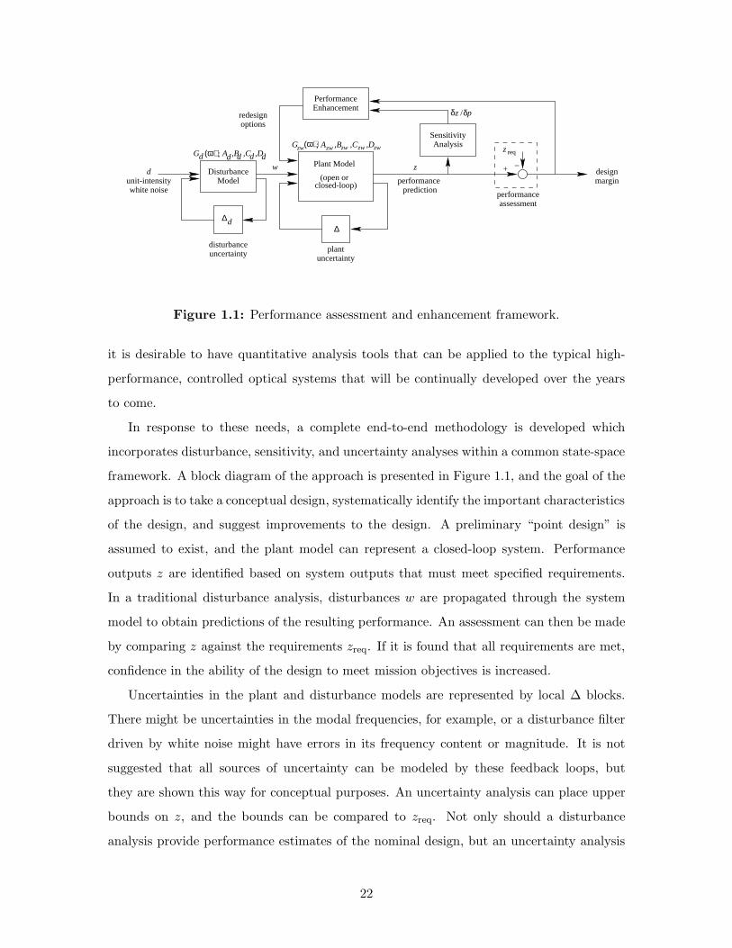
Figure 1.1: Performance assessment and enhancement framework.

it is desirable to have quantitative analysis tools that can be applied to the typical high-

performance, controlled optical systems that will be continually developed over the years

to come.

In response to these needs, a complete end-to-end methodology is developed which

incorporates disturbance, sensitivity, and uncertainty analyses within a common state-space

framework. A block diagram of the approach is presented in Figure 1.1, and the goal of the

approach is to take a conceptual design, systematically identify the important characteristics

of the design, and suggest improvements to the design. A preliminary “point design” is

assumed to exist, and the plant model can represent a closed-loop system. Performance

outputs z are identified based on system outputs that must meet specified requirements.

In a traditional disturbance analysis, disturbances w are propagated through the system

model to obtain predictions of the resulting performance. An assessment can then be made

by comparing z against the requirements zreq. If it is found that all requirements are met,

confidence in the ability of the design to meet mission objectives is increased.

Uncertainties in the plant and disturbance models are represented by local ∆ blocks.

There might be uncertainties in the modal frequencies, for example, or a disturbance filter

driven by white noise might have errors in its frequency content or magnitude. It is not

suggested that all sources of uncertainty can be modeled by these feedback loops, but

they are shown this way for conceptual purposes. An uncertainty analysis can place upper

bounds on z, and the bounds can be compared to zreq. Not only should a disturbance

analysis provide performance estimates of the nominal design, but an uncertainty analysis

22

should place the equivalent of “error bars” around znominal. The uncertainty analysis is

essentially a disturbance analysis that accounts for uncertainties.

Unsatisfactory results lead to a system improvement phase during which modifications

to the design are considered. The objective is to suggest modifications (e.g., applying

controlled structures technologies) that lead to acceptable design margins. A sensitivity

analysis can be used to identify the critical parameters to which the performance is most

sensitive, and these parameters can be targeted for redesign. The improvement phase ends

when a comfortable design margin exists, or when it is discovered that zreq can only be

satisfied if the uncertainty levels are reduced. A rigorous testing program which serves to

improve knowledge of the parameters should then be planned.

1.2 Research Objectives and Approach

The primary objectives of the research are summarized below.

• Develop a consistent and general methodology for assessing the performance of sys-

tems in which the structural dynamic and control aspects must be considered.

• Implement the methodology as a series of compatible analysis tools that are applied

to a nominal system model driven by disturbance models. The tools should consist of

– a disturbance analysis tool for predicting performance outputs,

– a sensitivity analysis tool for predicting changes in performance outputs due to

changes in model parameters, and

– an uncertainty analysis tool for estimating variations in the predicted perfor-

mance outputs due to uncertainties in model parameters.

• Identify computation and time-saving measures that permit the analysis tools to be

applied to large-order systems.

• Suggest an approach for performance enhancement that utilizes the analysis results

to identify design options with improved performance.

• Validate the analysis tools on various mathematical systems and on an experimental

testbed.

23

• Apply the overall methodology to an existing integrated model of the Space Interfer-

ometry Mission.

The approach that is taken to develop the end-to-end methodology is as follows. The

governing equations are derived and then implemented in MATLAB code. The code is ap-

plied to problems of different levels of complexity, beginning with simple, low-order models

that provide an understanding of the basic issues as well as help to validate the equations.

Then, the technique is applied to more complex models to investigate issues that might not

be readily apparent on the simple models. All of the analysis methods are designed to be

applied to the large-order, sophisticated models of systems that motivate this research. An

underlying theme is the development of model reduction and other approximation strategies

that permit results to be obtained in realistic time without significant loss of accuracy. The

product of this work is not only a conceptual methodology, but also a software toolbox that

has been tested and which is ready for application to real-world systems.

1.3 Literature Review

The research does build upon previous work in the different areas that are encompassed by

the assessment and enhancement framework. Creating the nominal plant and disturbance

models occurs during an integrated modeling process. A software package called IMOS

(Integrated Modeling of Optical Systems) [46] was developed at the Jet Propulsion Labora-

tory (JPL) to facilitate the generation of initial models of optical instruments. IMOS offers

the ability to significantly reduce the time required to take a concept of a system, build an

integrated model, and conduct analyses and trade studies. The need for such a capability

was described by Laskin and San Martin during a traditional design and analysis exercise

on the Focus Mission Interferometer [53].

Modeling precision optical systems requires fundamental knowledge of several distinct

disciplines. Structural dynamics is one field, and a popular textbook by Craig [13] offers a

good introduction. Since most structural dynamic models are based on the finite-element

method, the books by Bathe [5] and Cook [12] should be consulted. Another important

aspect of structural modeling is damping, and it is critical that realistic levels of damping

be used in the integrated models. In particular, the damping of structures at the small

vibration levels that are expected on precision spaceborne optical systems is an area that

24

has recently been investigated. The research by Ting and Crawley [84] and Ingham [39]

was motivated by the lack of experimental data at these low vibration levels.

The reliance of these systems on closed-loop control requires that actuators, sensors,

and compensators be included in the integrated model. Introductory textbooks such as

those by Van de Vegte [85] and Ogata [71] are useful for a review of classical control design

techniques, while that of Zhou et al. [88] emphasizes modern control theory approaches.

Since most control systems are implemented on digital computers, the standard references

by Astrom [1] and Franklin and Powell [22] are recommended.

Optical modeling is another area that is essential, and Redding and Breckenridge [78]

describe the mathematics behind linear ray trace theory. The main product of the optical

modeling process is a sensitivity matrix that relates perturbations in optical quantities such

as pathlength and beam walk to motion of the optical elements. A software program called

MACOS (Modeling and Analysis for Controlled Optical Systems) [45] creates the sensitivity

matrix based on a prescription of optical elements in the system. The optical sensitivity

matrix can be readily incorporated with a state-space representation of the structure and

control system.

Although disturbance modeling is often overlooked, its importance cannot be under-

stated. All potential disturbance sources that can hinder the performance of a high preci-

sion optical system need to be identified. Eyerman and Shea [20] provide a very complete

overview of spacecraft disturbances. Two specific disturbances that are anticipated to cause

problems for these systems are reaction wheel disturbances and thermal snap. Disturbance

characterization efforts related to both have been conducted in recent years. Bialke [6] offers

a good explanation of the sources of reaction wheel disturbances. The reaction wheels of the

Hubble Space Telescope, in particular, have been extensively analyzed [17], and Melody [60]

uses data from tests on a single wheel to derive a stochastic disturbance model. This model

serves as the basis for the development of a more general reaction wheel assembly (RWA)

disturbance model in Chapter 2. The relatively unknown effects of thermal snap prompted

experimental and modeling efforts in this area. Modeling thermal snap phenomena was

the subject of research by Kim [49]. The IPEX (Interferometry Program Experiment)

sequence of flight experiments was designed to quantify some of the thermal snap and as-

sociated microdynamics issues. IPEX-1 (STS-80, Dec. 1996) identified the microdynamic

characteristics of the Astro-Spas, a reusable spacecraft scientific platform, using a suite of

25

accelerometers [54]. IPEX-2 (STS-85, Aug. 1997) studied the representative dynamics of

a deployable, pre-loaded truss that was cantilevered from the Astro-Spas. Data suggests

the presence of thermal snap-like events that occur during orbital sun-shade transitions;

however, SIM-derived structural stability criteria are satisfied [55]. Efforts were also made

to use ground test data to quantify the magnitude of various disturbance sources on the

Astro-Spas (e.g., rate gyros, tape recorders, thrusters) [30]. Tests such as these should be

performed prior to launch of high performance optical systems.

Also of great use when creating large-order integrated models are methods for model

reduction. Creating a balanced state-space realization [65] can not only improve the nu-

merical conditioning properties of a model, but it also serves as a technique for identifying

states that can be eliminated from the model due to low observability and controllability

[88]. For the case of systems dominated by lightly-damped modes, the method proposed by

Gregory [27] is an efficient approach for ranking the importance of these modes.

The integrated modeling process is demonstrated by Melody and Neat [63] on JPL’s

Micro-Precision Interferometer testbed and is experimentally validated based on the com-

parison of predicted and measured closed-loop transfer functions. It is also demonstrated

by Shaklan et al. [79] on a SIM precursor design.

The theory behind conducting a stochastic disturbance analysis is well-developed.

Random vibration textbooks such as those by Crandall [14] and Wirsching [86] characterize

the response of systems driven by stochastic inputs in the time-domain (using autocorre-

lation functions) and equivalently in the frequency-domain (using power spectral density

functions). The concept of a linear shaping or “pre-whitening” filter whose input is white

noise and whose output is “colored” noise with desired magnitude and spectral content is

covered by Brown and Hwang [8]. For the case of state-space systems driven by white noise,

the output steady-state covariance matrix is known to be the solution of a Lyapunov equa-

tion [2]. These techniques are used extensively for performance assessment throughout this

thesis. Sample disturbance analysis results for space optical systems have been presented

for SIM [29],[32], an open-loop model of NGST [18], another proposed space interferometer

called POINTS [62], and a proposed Space Shuttle interferometry experiment called SITE

[15].

A sensitivity analysis provides useful information related to how dependent certain

quantities of a model are with respect to parameters of the model. Most sensitivities are

26

computed using a finite-difference approach; however, in certain instances, the sensitivities

can be calculated exactly. A goal of the sensitivity analysis framework in Chapter 4 is to

derive analytical expressions whenever possible and to avoid the inexact and often inefficient

finite-difference technique. A Lagrange multiplier approach is used by Jacques [40] to obtain

analytical sensitivities of a system’s outputs with respect to various parameters, and this

same methodology is employed in Chapter 4. The calculation of sensitivities with respect

to physical parameters requires mode shape and frequency derivatives, which fall under

the category of eigenvalue and eigenvector derivatives. (A good survey of various methods

is provided by Murthy and Haftka [66].) When the parameters are element mass and

stiffness properties of a finite-element model, these derivatives can be computed exactly

using methods developed by Fox and Kapoor [21] and Nelson [68]. Practical implementation

of these methods is done by Kenny [48], and this work is extended for use in Chapter 4.

The physical parameter sensitivity analysis framework derived in Chapter 4 for state-space

systems is similar to the approach used by Hou and Koganti [36] in the context of integrated

controls-structure design.

Past work relevant to the uncertainty analysis portion of the performance and en-

hancement framework includes the robust control design approach of Yang [87] and How

[37]. They derive estimates for bounds on a system’s H2 performance that are used in

the process of obtaining controllers that have stability and performance robustness to un-

certain modal frequencies. An approximate method for predicting worst-case performance

RMS values due to parametric uncertainties is that used by Bryson and Mills [9]. An ex-

haustive search of “corners” of the uncertain parameter space is conducted to identify the

combination of parameter bounds that results in the largest RMS value. From a structural

dynamics standpoint, the work by Hasselsman et al. [33], [34] provides different approaches

for estimating uncertainty in transfer function magnitude and phase due to uncertainties

in modal parameters. One particular method is the first-order approach that relates the

covariance matrix of output quantities in terms of the covariance matrix of uncertain param-

eters and the sensitivity matrix of the outputs with respect to the parameters. More general

treatment of model error and uncertainty from a control aspect is provided by Skelton [80]

and Zhou et al. [88]. Also applicable to the types of systems under consideration is the

work by Campbell and Crawley [10]. Modal parameter uncertainty models developed from

1-g tests are used to identify uncertainties in FEM mass and stiffness properties. These

27

uncertainties are propagated into modal parameter uncertainty models for the system in a

different environment (e.g., 0-g) or configuration.

Work in performance enhancement includes integrated control/structure optimiza-

tion. The objective is to develop structure and control designs simultaneously such that

the overall system design has improved properties compared to a system design obtained

through a traditional, sequential approach. This allows the same performance to be achieved

with less control effort or less structural mass, for example. The combined optimization can

be a challenging task, especially if the design parameters include stiffness/mass distribution,

structural connectivity/topology, actuator/sensor placement and type, and control design

parameters. Many of these options need to be fixed ahead of time to make the problem

formulation tractable for realistic systems. Solutions are dependent on the type of cost

functional specified and the solution technique employed. Jacques uses a typical section

approach to gain insight into the control/structure optimization problem [40]. The method

developed by Milman et al. [64] does not seek the global optimal design, but rather gen-

erates a series of Pareto-optimal designs that can help identify the characteristics of better

system designs. Masters and Crawley use Genetic Algorithms to identify member cross-

sectional properties and actuator/sensor locations that minimize an optical performance

metric of an interferometer concept [57]. The approach was experimentally validated on

a closed-loop, truss-like testbed [58], and this marks one of the few experimental investi-

gations into integrated control/structure optimization. Another example is the work done

at NASA Langley Research Center by Maghami et al. [56]. The pointing performance of

a large, laboratory testbed was successfully maintained while control effort was decreased.

Design parameters were controller gains and cross-sectional properties of groups of truss

elements. Topological redesign was performed by Keane on an open-loop, truss structure

to minimize the response in a truss member due to an external disturbance [47].

Performance enhancement on systems with uncertain parameters is treated by Parkinson

et al. [76] and Pritchard et al. [77]. The method by Parkinson et al. finds an optimal

design that satisfies specified constraints even when certain parameters are uncertain. It

is a two-step procedure whereby the nominal optimum design is determined first, then a

second optimization problem is solved whose constraints are modified by the uncertainties.

The effects of uncertainties are calculated based on a first-order approximation. Pritchard

et al. use a nested procedure in which an inner loop is a standard constrained optimization

28

problem and an outer loop searches for the optimum design whose performance is least

sensitive to specified parameters. Both methods are applied to and demonstrated on simple,

static structural problems.

Finally, Crawley et al. present a methodology for the conceptual design of controlled

structural systems [15]. It applies a controlled structures technology (CST) framework in

a consistent level of modeling detail. The goal is to identify the critical disturbance-to-

performance transmission paths and to determine the amount of CST options that are

required to achieve performance requirements.

1.4 Thesis Overview

Figure 1.2 is designed to provide a sense of the chronological order of the analyses. It also

serves as a thesis roadmap to help put the chapter sequence in context. Before any of the

performance assessment tools can be applied, a nominal model of the proposed system is

needed. For spaceborne systems such as SIM and NGST, an integrated modeling process

unifies structural dynamic, control, optics, and disturbance models. An overview of each

of these disciplines is offered in Chapter 2, and the SIM integrated model is used as a

representative example. Once the model is created, the disturbance analysis is conducted.

Chapter 3 describes time-domain, frequency-domain, and Lyapunov analyses that can be

used to estimate the nominal root-mean-square (RMS) values of the performance metrics.

The chapter also demonstrates how to identify the critical structural modes and distur-

bances from a frequency-domain analysis. A sensitivity analysis with respect to the modal

parameters of the critical modes is then performed, and details are provided in Chapter 4.

After the important modal parameters are identified, an uncertainty analysis predicts the

worst-case RMS values when the modal parameters are not known exactly but are bounded.

Chapter 5 develops a technique that solves a constrained optimization problem in order to

find the combination of uncertainties that maximizes the RMS values. When the results are

unsatisfactory, the performance enhancement phase is entered. Useful redesign options can

be identified by physical parameter sensitivities, and the basic theory is discussed in Chap-

ter 4. The parameters that affect the critical modes are selected for the sensitivity analysis,

and this process is also included in Chapter 4. Chapter 7 summarizes various options to

try during performance improvement efforts, and it includes an example application to the

29

performance assessmentphysical parametersensitivity analysis

z , critical modesnom

nomz + z∆

uncertainty analysis(modal domain)

modal parameter tophysical parameter mapping

important modalparameters

disturbance analysis

modal parametersensitivity analysis

comments

(c) requires state-space formulation [Chap. 4]

(b) 3 types (time-domain, freq.-domain, Lyap.) [Chap. 3]

important physicalparameters

(c)

sensitivities design margin

(d)

routine to identify worst-case parameters

[Chap. 5]

[Chap. 4]

[Chap. 7]

integrated modeling

nominal model

(a) integrates disturbance, structural, control, and optical models [Chap. 2]

(a)

(b)

(e)

(f)

(h)

frequency derivatives

unsatisfactory

(d) strain energy plots useful

(e) uses constrained optimization

(f) requires mode shape and

(g) applies CST methodology

(h) if performance

[Chap. 4,6]

performance enhancement process(g)

improveddesign

Figure 1.2: Analysis procedure.

SIM model. The results of an experimental validation exercise are found in Chapter 6.

30

Chapter 2

Integrated Modeling

This chapter discusses the integrated modeling approach as motivated by high precision

opto-mechanical space systems. Although the contributions in this thesis are primarily

related to the development and application of analysis tools, it will be seen that some of the

underlying assumptions are based heavily on the type of model being analyzed as well as the

type of inputs and outputs. In particular, the specific disciplines that are considered in the

modeling process are structural dynamics, controls, and optics. The inputs are stochastic

on-board disturbances, and the outputs are optical performance metrics expressed in a root-

mean-square (RMS) sense. The first section will explore these different areas of integrated

modeling a bit further. Section 2.2 will then describe the integrated model of the Space

Interferometry Mission that was developed at the Jet Propulsion Laboratory. This model

is frequently used in the other chapters to demonstrate the analysis tools on a realistic

system, and a better understanding of the model will help to put the results in perspective.

One contribution that is made in the modeling area is the creation of a multiple reaction

wheel disturbance model based on an existing model for a single wheel, and the details are

provided in Section 2.2.5.

2.1 Integrated Modeling Description

2.1.1 Motivation

As the next generation of space telescopes push the limits of achievable performance, initial

end-to-end system modeling will play a greater role in evaluating potential concepts. The

31

modeling and subsequent analyses will help to identify key trades and to assess the effec-

tiveness of various technologies. These high performance systems will rely on a number of

subsystems from different disciplines to help meet requirements. In response to this, models

will need to incorporate the disciplines in a unified approach.

For the purposes of this thesis, the term integrated modeling will refer to the process

of creating an overall input-output model of a system using modeling tools from a number

of distinct disciplines. The correct disciplines can be determined by first identifying what

the requirements are that must be satisfied. Then, aspects of the system should be isolated

which are needed to accurately predict the quantities on which the requirements are placed.

This can be accomplished based on previous modeling experience on similar systems, or

it might be an iterative process whereby more disciplines are added as they are deemed

important for greater predictive accuracy.

To illustrate this, consider the disciplines required for a model of a spaceborne observa-

tory such as an interferometer, which is the motivation for the work in this thesis. Inter-

ferometers typically have tight precision requirements on the phase, pointing, and overlap

differences of stellar light beams that are interfered together to produce the desired fringe

pattern [11]. Any deviation will lead to a reduction in fringe visibility, and dynamic ef-

fects in particular result in so-called “fringe blur.” A desired fringe visibility value can be

translated into requirements on errors such as pathlength difference. To be able to estimate

optical outputs, the integrated model must contain an optical model based on prescriptions

of the elements along the optical train. The elements such as mirrors and detectors are

attached to a supporting structure, so a structural model is needed. Since dynamic effects

are important, a structural dynamic model rather than just a static structural model is

required. This is especially true since the interferometer is on a flexible space structure

rather than a fairly rigid, ground-based support structure. The flexibility implies that the

optical requirements can probably not be met by relying solely on the passive rigidity of

the structure, so active optical control must be employed to control the light path. Thus, a

control system model should be incorporated as well. Finally, the spacecraft is not perfectly

“quiet,” and there are sources of disturbances that affect the interferometer’s ability to meet

the optical requirements. These disturbances should also be characterized and modeled.

Thus, the following disciplines have been identified as important in the integrated mod-

eling process of precision controlled optical systems.

32

• structural modeling

• control modeling

• performance (e.g., optical) modeling

• disturbance modeling

Each one will now be described in more depth.

2.1.2 Structural modeling

There are several tools available for modeling of structural systems, and they generally

are well developed. The most accepted standard is the finite-element method (FEM), and

this will be the assumed method of choice. This, of course, is case specific, and there

can be instances where the actual system being modeled can be better represented by a

different technique. For instance, an interferometer which has large slewing masses on a

flexible structure will require multi-body modeling techniques as well as standard FEM-

based structural dynamic models.

In the finite-element method, an important consideration is the level of fidelity and

discretization that is required. Early generation models of conceptual designs are more

useful if they can capture the essential physics of the system with a minimal amount of

complexity. This will help during the analysis phase when several types of analysis or trade

studies are required and computational effort can become an issue. The amount of fidelity

is usually dictated by the frequency range of importance, but this might not be identified

until after an initial model has been created and analyzed. Thus, some iteration is possible

before an appropriate amount of fidelity is reached. If the frequencies of interest are high,

then the fidelity might need to be increased; however, this leads to a larger order model,

and the predictive capability of an FEM might become an issue at these higher frequencies.

As an example of model fidelity, consider a long truss-like boom that is a component

of a structure. If only the first bending mode is particularly important in the performance

output of interest, then the truss can be modeled as a homogeneous beam comprised of

enough beam elements to yield a good estimate of the fundamental mode. This might

require only five elements as opposed to a number such as 100 (one for each strut in the

truss) which would be needed for a detailed model.

33

The fidelity and discretization issues not only affect the number of elements to use in the

model, but also what types of elements to use. For instance, plate-like components might

be part of the initial design, but frequency considerations could allow the components to be

treated as rigid bodies. Struts that are part of a truss could be modeled by rod elements

rather than Bernoulli-Euler beam elements.

Another aspect of structural modeling that is often not provided by an FEM approach

deals with structural damping. Unless there are discrete dampers present in a design,

the damping is typically specified in terms of modal damping ratios of specific modes. The

values are usually conservative (i.e., light damping in the range ζ = 0.1% – 0.5%), but efforts

should be made to choose damping ratios that are realistic rather than overly conservative

or overly ambitious. Specifying damping in this manner does require a structural model

in modal coordinates, and this raises the issue of how many modes should be kept in the

model.

Thermal modeling can also be placed under the generic heading of structural modeling.

If thermal effects are anticipated to cause thermal deformations of optical elements (such

as mirrors), and these deformations can contribute as much wavefront error as the dynamic

model, then a thermal model should be incorporated into the overall integrated model.

To be accommodated within the analysis framework proposed in this thesis, the final

result of structural modeling should be an input-output (i.e., state-space) system of the

form shown in Figure 2.1. Section 4.3.1 will provide further detail on how to create this

model based on standard structural dynamic equations expressed in modal coordinates.

F - Structuralmodel

- x

Figure 2.1: Open-loop system provided by structural modeling.

The vector F represents a generic force vector applied at all physical degrees of freedom.

A goal of disturbance and control modeling is to identify the degrees of freedom at which

the disturbances and control inputs actually enter. Note that this implies the structural

modeling process should keep in mind where control inputs act and where potential dis-

turbance sources enter. If the proper degrees of freedom are not exposed in the model,

then modifications will have to be made to accommodate these inputs. This can lead to

34

significant analysis delays if it is not done early in the model generation stage.

The vector x in Figure 2.1 represents all the physical degrees of freedom in the model.

A goal of performance and control modeling is to produce estimates of the performance

metrics and sensor outputs in terms of these quantities. Although not shown in Figure 2.1,

other outputs can be the velocity x and acceleration x if they are required.

Only some issues have been mentioned related to structural modeling, and in no way

is this brief discussion meant to address all of the requirements of the structural modeling

process. In fact, some systems might require a coupled-field formulation (e.g., structural-

acoustic coupling [25]), so the structural model block in Figure 2.1 would actually be re-

placed by a coupled-field model.

2.1.3 Control modeling

When a system relies on closed-loop control to improve its performance, it is the closed-

loop system that must be used during performance assessment. One option is to use simple

frequency-domain filters that approximate the effects of closed-loop control without actually

closing a loop in the model. This approach is used by Jandura when doing isolator trade

studies on a SIM model [42]. Another option that is more common is to model the controller

explicitly. This requires that a model of the control system be incorporated with the

structural model. In the most simplest form, the control model can consist of the three

additional components shown in Figure 2.2. A matrix Cyx maps the structural states into

the ideal sensor measurements y. A controller then takes these measurements and computes

a desired control input u applied by the actuators. The matrix βu then maps the control

inputs into forces and/or moments at the appropriate degrees of freedom in the structural

model. Note that the feedback used is shown as positive in Figure 2.2 since it is assumed

that the controller model incorporates any negative signs due to feedback. As an example,

consider a Linear-Quadratic-Gaussian (LQG) compensator. The control input u might be

defined as u = −Gx, where G is the Linear Quadratic Regulator (LQR) feedback gain and

x is the state estimate produced by a Kalman filter [88]. In this case, think of the quantity

βuu as being the actual physical forces and/or moments applied to the structure.

This simple representation of the control system in Figure 2.2 is often adequate dur-

ing a conceptual design phase to examine the benefits and top-level issues of control. The

controller can be represented by a continuous-time state-space filter even though the actual

35

Fg - Structural

model

Controller

Cyxβu

x-

?6

6

-+

+0

u y

Figure 2.2: Additions made by control modeling.

control system will be implemented in discrete form in a computer. The linear, state-space

assumption made in the subsequent chapters is not too restrictive since many control ap-

proaches can lead to a control model in this form. What should be kept in mind, though,

is that a realistic controller should be used when evaluating the performance of the over-

all system. For instance, a controller design that achieves good performance at the cost

of minimal phase margin would probably lead to instability when implemented in digital

form at realistic sampling rates. The original performance predictions would therefore be

misleading. As another example, consider a model-based compensator that utilizes precise

knowledge of the modal frequencies to achieve many dB of performance improvement. The

robustness to errors in the model would more than likely be very poor, and the performance

predictions would again be unrealistic.

There are a number of other issues related to control modeling that should be consid-

ered in terms of potential importance to fair and accurate system assessment. Figure 2.2

makes the assumption that the sensors provide perfect measurements and that the actuators

provide the exact control inputs. This ignores the fact that actual sensors and actuators

have internal dynamics and limited range and resolution, and these might lead to perfor-

mance limitations. The controller design should take these into account either explicitly

(such as with appended dynamics to the model) or implicitly (by using realistic gains and

bandwidths).

Some issues pertaining to digital control implementation include time delay, quantiza-

tion, signal processing, and computational precision. A model of time delay can easily be

added in the form of a Pade approximation to the control model in order to keep the con-

trol design “honest.” For the case of high performance systems that push the limits of the

36

current state of the art, issues such as these might need to be accounted for at some level

early in the conceptual design. For other systems, however, these effects can typically be

added at later stages when the design and the models are more mature.

A last item associated with real control systems involves sensor and actuator noise,

which can also place limitations on performance. These are better classified and modeled

as disturbances, so they will be mentioned again in the disturbance modeling section.

2.1.4 Performance modeling

Although at first glance it might appear to be the easiest of the modeling tasks to do,

modeling the performance of a system can be quite challenging. This is especially true

for the complicated, high performance systems being considered in this thesis. The aim of

performance modeling is to provide the relation between states in the model and metrics

on which requirements are placed. This is shown in Figure 2.3 as the matrix Czx, which

expresses the performances z as a linear combination of the states x.

Fg - Structural

model

Controller

Cyxβu

xCzx

z--

?6

6

-+

+0

u y

Figure 2.3: Addition made by performance modeling.

The success of a system is usually defined in terms of its ability to achieve certain goals.

For a space interferometer, a goal might be to achieve a desired level of accuracy when

measuring the angular separation between stars of a specified stellar magnitude. A high-

level requirement such as this is often not directly associated with the performance outputs

in z. What is normally done in practice is to flow down the high-level requirements into

requirements on quantities that can be directly predicted by the integrated model. For

instance, the requirements flowdown approach can levy a 1 nm requirement on optical path

difference (OPD) for the interferometer case.

The most difficult and often least rigorous part of performance modeling is this flowdown

37

process. An error budget tree is usually created, and requirements on subsystems are

normally allocated in an ad hoc fashion. If design decisions and resource allocation are

based on an unrealistic requirement, then the final system design might be quite inefficient.

Efforts should be made to iterate on the requirements based on preliminary analyses so that

a more reasonable allocation is achieved.

Once requirements are placed in terms of quantities that the integrated model can

address, then the next step is to determine how to obtain the quantities from the model.

This can be straightforward if the requirements are on physical displacements, velocities, or

accelerations of points on the structure. For the case of optical systems, the requirements

will be on optical quantities, and these are inherently dependent on motion of the optical

elements. An additional optical modeling process is needed that provides an estimate of

the effect of this motion.

The analysis framework to be discussed in the following chapters assumes that the

transformation from structural displacements to performance quantities is linear. It can

simply be a Czx matrix as shown in Figure 2.3, or it can be represented by a linear dynamic

system if frequency weighting is used. The use of a linear performance model might not

be valid in some situations, and this is an issue that must be addressed further when

encountered.

If there are multiple performance outputs (i.e., z is a vector), then whenever possible,

a weighting matrix should be applied to z and an appropriate norm should be calculated

to produce a scalar performance cost. For instance, weightings can be incorporated in a

matrix R, and the weighted performance outputs can be denoted by z.

z = Rz (2.1)

A scalar cost J can then be defined as a norm of z

J = ||z|| (2.2)

and the weighting matrix R can be absorbed into the Czx matrix.

For the types of systems of interest, the performance requirements will generally be

specified in terms of RMS values, which is a 2-norm (i.e., an H2 measure).

38

2.1.5 Disturbance modeling

The last major task of the integrated modeling process is to characterize the disturbances

w. A key step in creating a disturbance model is specifying the locations on the system at

which the physical disturbances act, and this is captured by βw in Figure 2.4. As mentioned

previously, sensor and process noise can corrupt y and u as well, but these disturbances

are not explicitly shown. The remaining discussion regarding disturbance modeling will

emphasize ways to identify and characterize the disturbances w.

Fg - Structural

model

Controller

Cyxβu

xCzx

z--

?6

6

-βw-w

++

u y

Figure 2.4: Addition made by disturbance modeling.

When assessing the impact of disturbances on high-performance systems, it is critical

that the disturbance models be fairly representative of the actual disturbances. An ex-

tremely accurate plant model can still produce erroneous results when improperly modeled

disturbances are applied to it. If design trades and decisions are based on the results of

disturbance analyses that use mismodeled disturbances, then the performance of the actual

system in operation might be quite different from that which was predicted. As a result,

the disturbance characterization process should be given as high a priority as the integrated

modeling process. This is especially true for high performance systems in which even low

disturbance levels can cause the response to exceed requirements.

The types of disturbances that can affect a system are numerous, and spacecraft in par-

ticular face a myriad of them [20]. Table 2.1 lists some potential disturbances, and they are

classified depending on whether the disturbance source is the space environment (external)

or a component of the spacecraft (internal). The frequency range column indicates the

approximate frequencies at which the disturbances acts.

Disturbances can be quantified by their frequency content, magnitude level, and the

39

Table 2.1: Listing of some spacecraft disturbances.

Disturbance Frequency Description

External

gravity gradienttorque

low nonuniform gravitational field acting on dis-tributed body

atmospherictorque

low center of pressure 6= center of mass

magnetic torque low net spacecraft magnetic dipole not alignedwith external magnetic flux

solar pressuretorque

low center of pressure 6= center of mass

solar thermal flux low can cause thermal deformation (static re-sponse) and thermal snap (high freq. re-sponse) during transients (e.g., sun-shadetransition)

Internal

RWA/CMG mid/high series of harmonic disturbances (due to im-balances, bearings, motor ripple and cogging,etc.) that are functions of wheel speed

thrusters low/mid/high on/off cycling causes impulse-like or step-like disturbances (due to propellant expulsionand/or valve operation)

fluid slosh low/mid excitation of propellant or coolant sloshmodes in storage tanks causes motion ofspacecraft

fluid flow low/mid/high propellant or coolant flow and valve operation

servomechanisms low/mid/high drive motor disturbances (e.g., friction, cog-ging, ripple in antenna/solar array gimbals,ODL trolley)

tape recorders low/mid/high motion of mechanisms during operation

rate gyros mid/high one or more harmonic disturbances due to im-balances in spinning elements

thermal control low/mid mechanisms in cryocooler pumps, louvers

sensor noise low/mid/high bandwidth/resolution limitations, A/D quan-tization, electrical noise, etc.

actuator noise low/mid/high bandwidth/resolution limitations, D/A quan-tization, electrical noise, etc.

40

location and direction at which they enter the structure. The frequency content determines

which modes of the structure can be excited and what the bandwidth of a control system

should be. The magnitude level determines how much energy enters the structure. The

location and direction information determine to what extent the modes in the frequency

range can be excited. This is the disturbability notion from modern control theory, or

the modal force notion from structural dynamics. Both can be expressed in terms of the

quantity ΦTβw, where Φ is the modal matrix and βw is the disturbance influence matrix

which maps the disturbances w to the physical DOF’s. If φi is the ith mode in the matrix

Φ, then φTi βw = 0 implies that the ith mode is not disturbable by w since the modal force

is zero. This arises, for example, when a point force is acting at a location which is a node

(zero displacement) for a particular mode of the structure.

Disturbances are also characterized by whether they are stochastic (i.e., random) or

deterministic in nature. A deterministic signal is one which can be predicted exactly during

the time interval of importance. For example, the harmonic signal w(t) = 2 sin 5.2t is

known exactly for any desired time t. Stochastic processes can be deterministic in form,

yet can have some random element. The signal w(t) = 2 sin(5.2t+ φ), where φ is a random

phase angle between 0 and 2π, is an example. Stochastic processes can also be completely

nondeterministic in form, such as is the case with most sources of sensor noise.

The deterministic vs. stochastic classification can be illustrated with some of the dis-

turbances listed in Table 2.1. Servomechanisms, for instance, can lead to deterministic

disturbances. A desired motion of an antenna will require a certain torque, and the reac-

tion torque can be thought of as a disturbance. The drive motors used in servomechanisms

can also introduce a stochastic component due to electromechanical noise. Solar pressure

torque can be calculated deterministically based on parameters such as the distance from

the spacecraft to the Sun, and the absorptivity and reflectance coefficients [50].

Most of the external spacecraft disturbances can lead to internal disturbances. These

external disturbances are usually in the form of torques, and ACS actuators (reaction wheels,

CMG’s, or thrusters) that counteract these in order to maintain pointing requirements can

produce other unwanted forces and moments, generally at higher frequencies. Another

example is when a sudden change in solar thermal flux leads to on-board thermal snap

events due to a spontaneous release of stored strain energy. In these situations, a decision

needs to be made regarding whether to ignore the external disturbances or to model them

41

explicitly, along with the system’s response to them. For instance, a gravity gradient torque

can be explicitly modeled as an exogenous disturbance, and ACS control loops that are in

the spacecraft model can send the appropriate command signals to the reaction wheels. A

reaction wheel model which contains as its output the resulting desired torque might also

include the disturbance forces and torques that arise.

It might be difficult to create an overall model that is driven by external disturbance

estimates and which produces the corresponding internal disturbances. If the external

disturbances are ignored, then one option is to assume typical time histories of the internal

disturbances based on experience. For example, a thruster firing profile can be created

that is typical during station-keeping mode. For the reaction wheel assembly case, typical

wheel speed profiles can be assumed, and the resulting wheel-speed-dependent disturbance

time histories w(t) can be generated. A potential problem with this approach is that if

the sample disturbance time history is not really representative of what can arise during

the course of a mission, then multiple analyses need to be conducted that use a series of

these sample time histories. If the disturbances are stochastic in nature, then this process

can be avoided by using random process theory. “Expected” levels of response can then be

predicted by conducting a single analysis; however, a drawback is that worst-case conditions

or transient effects might not be identified.

Since disturbances will be modeled primarily as stochastic throughout this thesis, a

brief review of the pertinent theory of random processes will now be presented. Certain

stochastic processes can be characterized by their so-called correlation and spectral density

functions, which in general can be matrices. The correlation function of the random process

w(t) is defined as

Rww(t1, t2) = E[w(t1)wT (t2)

](2.3)

where E[·] is the expectation operator. If w(t) is stationary (i.e., the statistics of w do not

change in time), then Rww is a function of a single time-lag variable τ .

Rww(τ) = E[w(t)wT (t+ τ)

](2.4)

The covariance matrix Σw will be defined (for zero-mean processes) as the value of the

42

correlation matrix at τ = 0.

Σw = Rww(0) =

w21 w1w2 · · · w1wn

w2w1 w22 · · · w2wn

......

. . ....

wnw1 wnw2 · · · w2n

=

σ2w1

σw1w2 · · · σw1wn

σw2w1 σ2w2

· · · σw2wn

......

. . ....

σwnw1 σwnw2 · · · σ2wn

(2.5)

where n is the total number of elements in the vector w, and the notation (·) is analogous

to the expectation operator. To see why this simplification can be made for zero-mean

processes, consider a typical term σwiwj in the covariance matrix.

σwiwj = (wi − wi) (wj − wj)

= wiwj − wiwj − wiwj + wi wj

= wiwj − wi︸︷︷︸=0

wj︸︷︷︸=0

= wiwj (2.6)

The mean-square values of the elements of w are simply the diagonal entries in the covariance

matrix.

(Σw)i,i = E[w2

i (t)]≡ w2

i (2.7)

where wi(t) is the ith element in w. If w is zero-mean, then the mean-square values and

the variances are identical. For simplicity, all stochastic processes will be considered to have

zero mean. This assumption will be valid throughout this thesis.

σ2wi

= E[w2

i (t)]− (E [wi])

2︸ ︷︷ ︸=0

= w2i (2.8)

Taking the Fourier transform of Eq. 2.4 produces the spectral density function Sww(ω)

[8].

Sww(ω) = F [Rww(τ)]

≡∫ +∞

−∞Rww(τ)e−jωτ dτ (2.9)

43

Notice that the factor 12π is not included in this definition of the Fourier transform. Other

definitions (e.g., [86]) do place this factor in the Fourier transform formula. Either definition

will produce the same results in the end as long as the definition is used consistently.

The inverse Fourier transform of Sww(ω) recovers the correlation function.

Rww(τ) = F−1 [Sww(ω)]

≡ 12π

∫ +∞

−∞Sww(ω)e+jωτ dω (2.10)

Evaluating Eq. 2.10 at τ = 0 will produce the covariance matrix of w.

Σw =12π

∫ +∞

−∞Sww(ω) dω (2.11)

Eq. 2.11 suggests an alternative approach to calculating the mean-square values of w if the

spectral density functions are available, namely

σ2wi

= [Σw]i,i =12π

∫ +∞

−∞[Sww(ω)]i,i dω (2.12)

As a matter of terminology, the diagonal elements of the spectral density function matrix

are usually referred to as power spectral densities (PSD’s). Eq. 2.12 states that the variance

is equal to the area beneath the PSD scaled by a factor of 12π . In engineering practice, a PSD

is typically plotted versus a frequency axis with units in Hz. Making the transformation

ω = 2πf in Eq. 2.12 yields

σ2wi

=∫ +∞

−∞[Sww(f)]i,i df (2.13)

This is a powerful result that will be utilized quite often when frequency-domain disturbance

analyses are performed.

2.1.6 Numerical conditioning

An often overlooked aspect of integrated modeling deals with numerical conditioning. Large-

order models, in particular, can suffer from poor numerical conditioning if they are created

without measures that address this issue. Analysis results can be inaccurate if they are

based on a model with a bad numerical representation.

Since integrated models are assumed to be in state-space form, a balancing transforma-

tion can be used to convert the system into a balanced realization. (This will be described

in more detail in Section 5.3.1.) It is well known that different state representations of

a system can still produce the same input-output relationship. Some representations can

44

be better numerically conditioned than others, as measured by the condition number of

the state dynamics matrix A. A balanced realization typically yields a system that has an

improved numerical behavior.

One example of a situation that can lead to poor numerical conditioning is when a

compensator is designed using classical loop-shaping techniques. The compensator is nor-

mally in transfer function form and then converted to state space form via a canonical

representation [23]. If the compensator has more than a few states, then the coefficients

in the denominator of the transfer function can be fairly large. For instance, a canonical

representation of the fourth-order transfer function

u(s)y(s)

= G(s) =1

(s+ 4)(s + 10)(s + 40)(s + 100)

=1

s4 + 154s3 + 6000s2 + 61600s + 160000(2.14)

is given by

x =

−154 −6000 −61600 −160000

1 0 0 0

0 1 0 0

0 0 1 0

x+

1

0

0

0

y

u =[

0 0 0 1]x (2.15)

The condition number of the A matrix is 1.84 × 105. The condition number of a matrix

is defined as the ratio of the largest singular value to the smallest singular value. Nearly-

singular matrices are characterized by a large condition number. The technique described

by Moore in [65] can be used to obtain a balanced realization of the state-space equations

in Eq. 2.15. The “balanced” system of equations is then given by

˙x =

−1.445 4.131 1.613 0.4202

−4.131 −9.246 −9.766 −2.356

1.613 9.766 −37.41 −19.7

−0.4202 −2.356 19.7 −105.9

x+

−0.003341

−0.003807

0.001888

−0.0004856

y

u =[−0.003341 0.003807 0.001888 0.0004856

]x (2.16)

This time the condition number of the A matrix is 38.9, and this represents a significant

improvement in the numerical conditioning of the model. Thus, one recommendation that

45

can be made is that compensator state-space representations should be balanced if they are

obtained from transfer function form.

Examining Eq. 2.16 further leads to another recommendation. From a numerical preci-

sion or model reduction standpoint, it is often advantageous if the transfer functions from

the inputs to the outputs have numerical values of similar order of magnitude. To achieve

this, the units of the inputs and outputs should be scaled. For instance, if one of the out-

puts of an interferometer model is OPD, the natural unit of the output might be µm or

nm rather than the typical unit of meters. This allows the entries in the Czx matrix to be

changed by factors of 106 or 109, thereby addressing numerical precision limitations.

Transforming a system into a balanced realization can also help in model reduction, as

will be seen in Section 5.3.1. A balanced realization is useful in identifying unobservable

or uncontrollable states which can be removed from the model. Obtaining a minimal-order

model from an initial non-minimal order model is another useful step in improving the

numerical conditioning of a system.

Thus, numerical conditioning of integrated models should be considered in as much

detail as the actual modeling process. A few recommendations have been provided that

make an effort to avoid some potential pitfalls related to this issue, especially when dealing

with large-order systems.

2.2 Space Interferometry Mission Overview

The Space Interferometry Mission (SIM) will be one of the first-generation of missions that

are being planned as part of NASA’s Origins Program [81]. The Origins Program seeks

to answer some fundamental questions related to the birth and early evolution of galaxies,

stars, and planets [74]. Another objective is the search for potential life-sustaining planets

outside of our solar system. SIM is just one of a series of missions shown in Figure 2.5 that

will collectively attempt to provide answers to these questions.

This section will begin with the specific objectives of SIM and will provide an overview

of its operation. Then the integrated model of SIM that was developed at JPL will be

described in detail. The section will conclude with a rigorous development of a disturbance

model of a general reaction wheel assembly.

46

Figure 2.5: Timeline of Origins Program missions [43].

Figure 2.6: SIM Classic concept [44].

47

2.2.1 Modes of operation

SIM is an optical interferometer that can operate in one of several modes during scientific

observations. It consists of a series of seven discrete, separated apertures used to collect

the incoming starlight, and these are clearly visible in Figure 2.6. The concept shown in

Figure 2.6 will be referred to as SIM Classic, and it will be the concept on which many of

the analysis tools developed in this thesis will be demonstrated. Subsequent trade studies

at JPL have produced alternative architectures; however, these will not be described, and

their analysis will be left for future work.

One of the benefits of interferometry for space-based applications is that it can achieve

significant improvements in angular resolution without facing the same cost, mass, and

technical issues that could cause larger aperture telescopes to be infeasible with current

funding, launch vehicles, and technology. The basic premise behind interferometry is to

coherently interfere light from a pair of distributed apertures to produce interference fringes.

Scientific information can then be derived from the resulting fringe. Phase information is

related to the position of the fringe, and amplitude information is related to the visibility

of the fringe. Figure 2.7 includes some of the important elements required by a SIM-like

interferometer. The two collecting apertures, which are commonly called siderostats, are

used to point at a target of interest by means of a 2-axis gimbal. The light is redirected

into the instrument and follows a path through the optical train until arriving at a beam

combiner. Also shown in the figure is the path traveled by an internal metrology beam,

which is used to measure internal pathlength changes due to motion of the optical elements.

A layered control approach is used while the interferometer is in operation so that point-

ing and pathlength requirements can be met [53]. Pointing control is distributed among the

spacecraft attitude control system (ACS), siderostat pointing mechanisms, and fast steer-

ing mirrors (FSM’s). The ACS provides large angle, low bandwidth control, the siderostats

provide coarse angle, medium bandwidth control, and the FSM’s provide high resolution,

high bandwidth control. Photos of a commerically available gimbal-mounted mirror and

fast steering mirror are shown in Figure 2.8. The pathlength control is distributed in a

similar fashion; however, it is accomplished within the same unit, which is known as an

optical delay line (ODL). Large path delay (up to approximately 1 meter) is introduced by

using a belt-drive mechanism to translate the ODL along a trolley. This is performed at

48

#1siderostat

ODL introducesinternal pathdelay

fringe detector

Baseline B

common stellar wavefront= Bcos

stellar light

internal metrology

θ

θ

External path delay

siderostat#2

Figure 2.7: Schematic of the basic elements of an interferometer.

49

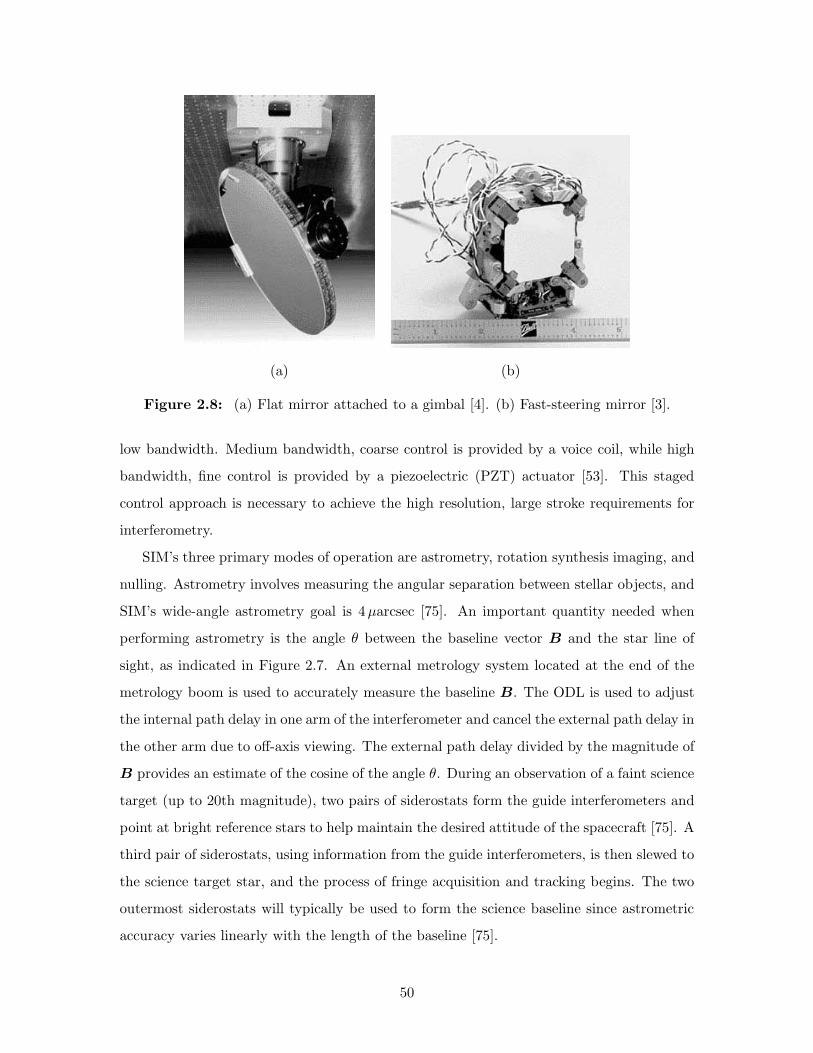
(a) (b)

Figure 2.8: (a) Flat mirror attached to a gimbal [4]. (b) Fast-steering mirror [3].

low bandwidth. Medium bandwidth, coarse control is provided by a voice coil, while high

bandwidth, fine control is provided by a piezoelectric (PZT) actuator [53]. This staged

control approach is necessary to achieve the high resolution, large stroke requirements for

interferometry.

SIM’s three primary modes of operation are astrometry, rotation synthesis imaging, and

nulling. Astrometry involves measuring the angular separation between stellar objects, and

SIM’s wide-angle astrometry goal is 4µarcsec [75]. An important quantity needed when

performing astrometry is the angle θ between the baseline vector B and the star line of

sight, as indicated in Figure 2.7. An external metrology system located at the end of the

metrology boom is used to accurately measure the baseline B. The ODL is used to adjust

the internal path delay in one arm of the interferometer and cancel the external path delay in

the other arm due to off-axis viewing. The external path delay divided by the magnitude of

B provides an estimate of the cosine of the angle θ. During an observation of a faint science

target (up to 20th magnitude), two pairs of siderostats form the guide interferometers and

point at bright reference stars to help maintain the desired attitude of the spacecraft [75]. A

third pair of siderostats, using information from the guide interferometers, is then slewed to

the science target star, and the process of fringe acquisition and tracking begins. The two

outermost siderostats will typically be used to form the science baseline since astrometric

accuracy varies linearly with the length of the baseline [75].

50

During the imaging mode, SIM rotates about the line of sight to the object and takes

u− v measurements by alternating between pairs of siderostats to create baselines of differ-

ent lengths and orientations. As in the astrometry mode, two guide interferometers track

bright stars as the third interferometer makes the necessary measurements on the target.

At each orientation, amplitude and phase information is obtained from the fringe position

and visibility, and a posteriori data processing synthesizes the actual image from the mea-

surements in the u − v plane [75]. Since the maximum baseline is 10 meters, an angular

resolution is achieved that is several times better than that of the Hubble Space Telescope.

The nulling mode is used during imaging when light from a very bright star would

otherwise hide any neighboring planets. In this case, the science light is sent to a nulling

beam combiner, which introduces a 180 phase shift to light in one arm of the interferometer.

This phase shift is designed to null the light arriving exactly down the line of sight by a

factor of 110000 [75]. This provides a means of direct planet detection, which is in contrast to

indirect techniques which infer the existence of an orbiting planet based on a parent star’s

“wobble,” for example.

Each of these operational modes has a unique set of requirements that must be met for

successful operation. As motivated earlier, such a complicated system requires an integrated

modeling approach for performance assessment. The structural, optical, and control models

will now be discussed in depth.

2.2.2 Finite-element model

The SIM finite-element model was created at JPL using the Integrated Modeling of Optical

Systems (IMOS) software package [46]. IMOS is a set of MATLAB functions that offer

the capability for structural dynamic, optical, control, and thermal modeling. An attrac-

tive feature of IMOS is that it can be used to create complete end-to-end models within

one computational environment. This facilitates trade studies and other analyses of early

generation system concepts.

Figure 2.9(a) shows the stick representation of the finite-element model of SIM. Node

locations are represented by circles, and elements are represented by line segments. Fig-

ure 2.9(b) shows the ray trace of stellar light passing through one arm of a guide inter-

ferometer. The siderostat booms and the metrology boom are modeled by Bernoulli-Euler

beam elements. Each of the two siderostat booms is considered to be a box beam and is

51

(a) (b)

Figure 2.9: (a) SIM finite-element model. (b) Ray trace through +x arm of guide#1 interferometer.

discretized using 15 nodes. Rigid elements attach the 7 siderostat center-of-mass nodes to

neighboring nodes on the siderostat boom. Rigid elements also attach various mirrors to

the support structure. The metrology boom is represented simply as a thin walled cylinder

and is discretized using 10 nodes. The beam launchers at the end of the metrology boom

are accounted for by a lumped, rigid-body mass [42].

The optics boom is treated as a rectangular rigid body with a total mass of 1200 kg.

Attached to it via rigid elements are 8 beam combiner nodes, 8 upper switchyard mirror

nodes, 8 lower switchyard mirror nodes, 8 fold mirror nodes, and 8 ODL center-of-mass

nodes.

Attached to one of the nodes along the optics boom is a coincident node at which the

reaction wheel assembly (RWA) is located. The two nodes are joined by an ideal hexapod

isolator model that represents a Stewart platform configuration of six struts [82]. When the

struts are perfectly pinned at their ends and are modeled by six identical axial springs with

stiffness k, the resulting stiffness matrix can be shown to be diagonal and in terms of the

52

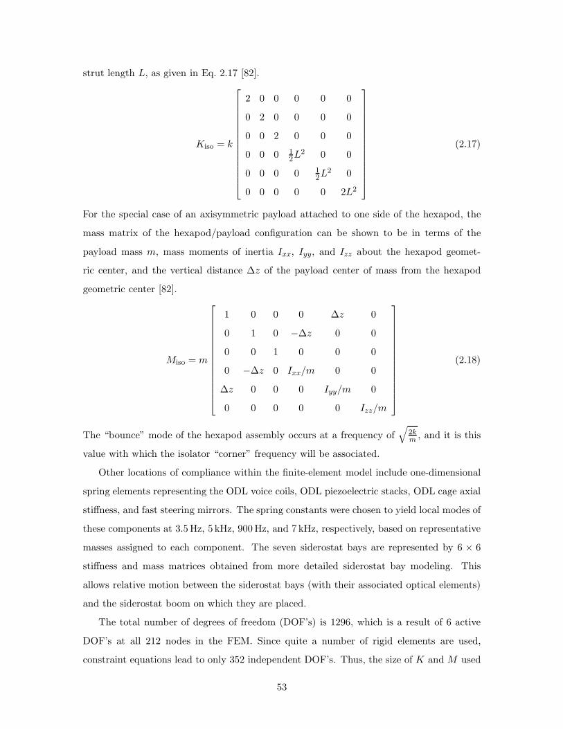
strut length L, as given in Eq. 2.17 [82].

Kiso = k

2 0 0 0 0 0

0 2 0 0 0 0

0 0 2 0 0 0

0 0 0 12L

2 0 0

0 0 0 0 12L

2 0

0 0 0 0 0 2L2

(2.17)

For the special case of an axisymmetric payload attached to one side of the hexapod, the

mass matrix of the hexapod/payload configuration can be shown to be in terms of the

payload mass m, mass moments of inertia Ixx, Iyy, and Izz about the hexapod geomet-

ric center, and the vertical distance ∆z of the payload center of mass from the hexapod

geometric center [82].

Miso = m

1 0 0 0 ∆z 0

0 1 0 −∆z 0 0

0 0 1 0 0 0

0 −∆z 0 Ixx/m 0 0

∆z 0 0 0 Iyy/m 0

0 0 0 0 0 Izz/m

(2.18)

The “bounce” mode of the hexapod assembly occurs at a frequency of√

2km , and it is this

value with which the isolator “corner” frequency will be associated.

Other locations of compliance within the finite-element model include one-dimensional

spring elements representing the ODL voice coils, ODL piezoelectric stacks, ODL cage axial

stiffness, and fast steering mirrors. The spring constants were chosen to yield local modes of

these components at 3.5 Hz, 5 kHz, 900 Hz, and 7 kHz, respectively, based on representative

masses assigned to each component. The seven siderostat bays are represented by 6 × 6

stiffness and mass matrices obtained from more detailed siderostat bay modeling. This

allows relative motion between the siderostat bays (with their associated optical elements)

and the siderostat boom on which they are placed.

The total number of degrees of freedom (DOF’s) is 1296, which is a result of 6 active

DOF’s at all 212 nodes in the FEM. Since quite a number of rigid elements are used,

constraint equations lead to only 352 independent DOF’s. Thus, the size of K and M used

53

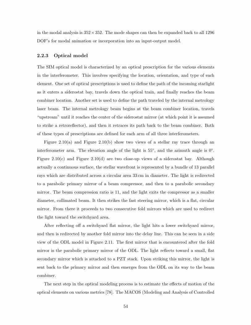
in the modal analysis is 352×352. The mode shapes can then be expanded back to all 1296

DOF’s for modal animation or incorporation into an input-output model.

2.2.3 Optical model

The SIM optical model is characterized by an optical prescription for the various elements

in the interferometer. This involves specifying the location, orientation, and type of each

element. One set of optical prescriptions is used to define the path of the incoming starlight

as it enters a siderostat bay, travels down the optical train, and finally reaches the beam

combiner location. Another set is used to define the path traveled by the internal metrology

laser beam. The internal metrology beam begins at the beam combiner location, travels

“upstream” until it reaches the center of the siderostat mirror (at which point it is assumed

to strike a retroreflector), and then it retraces its path back to the beam combiner. Both

of these types of prescriptions are defined for each arm of all three interferometers.

Figure 2.10(a) and Figure 2.10(b) show two views of a stellar ray trace through an

interferometer arm. The elevation angle of the light is 55, and the azimuth angle is 0.

Figure 2.10(c) and Figure 2.10(d) are two close-up views of a siderostat bay. Although

actually a continuous surface, the stellar wavefront is represented by a bundle of 13 parallel

rays which are distributed across a circular area 33 cm in diameter. The light is redirected

to a parabolic primary mirror of a beam compressor, and then to a parabolic secondary

mirror. The beam compression ratio is 11, and the light exits the compressor as a smaller

diameter, collimated beam. It then strikes the fast steering mirror, which is a flat, circular

mirror. From there it proceeds to two consecutive fold mirrors which are used to redirect

the light toward the switchyard area.

After reflecting off a switchyard flat mirror, the light hits a lower switchyard mirror,

and then is redirected by another fold mirror into the delay line. This can be seen in a side

view of the ODL model in Figure 2.11. The first mirror that is encountered after the fold

mirror is the parabolic primary mirror of the ODL. The light reflects toward a small, flat

secondary mirror which is attached to a PZT stack. Upon striking this mirror, the light is

sent back to the primary mirror and then emerges from the ODL on its way to the beam

combiner.

The next step in the optical modeling process is to estimate the effects of motion of the

optical elements on various metrics [78]. The MACOS (Modeling and Analysis of Controlled

54

−6 −4 −2 0 2 4 6−2

0

2

4

6

8

10

x

y

−2 0 2 4 6 8 10−6

−5

−4

−3

−2

−1

0

1

2

3

4

yz

(a) (b)

3 3.5 4 4.5

−0.8

−0.6

−0.4

−0.2

0

0.2

0.4

0.6

−1 −0.5 0 0.5 1−0.4

−0.2

0

0.2

0.4

0.6

0.8

1

(c) (d)

Figure 2.10: (a) Bottom view of ray trace. (b) Side view of ray trace. (c) Bottomview of ray trace through siderostat bay. (d) Side view of ray tracethrough siderostat bay.

55

−1 −0.5 0 0.5 1−4

−3.5

−3

−2.5

−2

−1.5

−1

Figure 2.11: Side view of ray trace through ODL assembly.

Optical Systems) program is used to create a linear model in the form of an optical “C”

matrix, which maps element motion into metrics such as pathlength, tilt, and spot motion

[45]. The outputs are for each of the rays in the light bundle, and the metrics for the bundle

as a whole are obtained by averaging over the rays. The main product of optical modeling

is this sensitivity matrix, and it allows optical control loops to be closed and optical-related

performance predictions to be made.

2.2.4 Optical control

The block diagrams in Figure 2.12 show two types of control loops that are implemented

in the SIM integrated IMOS model. Figure 2.12(a) represents the pathlength control ar-

chitecture, which consists of three compensators: Kvc (ODL voice coil), Kpzt (ODL piezo),

and Kft (fringe tracker). The outer loop is closed during fringe tracking mode once the

white-light fringe has been acquired. (Note: The fringe acquisition process is not explicitly

modeled, but the outer loop can be broken to examine the OPD levels due to disturbances.)

It is assumed that the ODL trolley has been locked in place once the fringe is acquired;

therefore, ODL trolley control is not shown. A CCD detector in the beam combiner mea-

sures the interference fringe position, which is related to the actual total OPD. In the block

56

Kft

Kvc

Kpzt Gpzt

Gvc

internal metrology

0 +

-

ext.OPD

disturb.disturb.OPDint.

totalOPD

+ +

+ +

+

+

+

ODLcontroller

fringe trackercontroller

-

plant

(a)

+

-

controller plant

r

+

+Kacs Gacs

ACS

attitude

Gd

disturb.

(b)

Figure 2.12: (a) Block diagram of ODL and fringe tracker controllers. (b) Blockdiagram of ACS controller.

diagram, this measurement is assumed to be ideal, and practical considerations such as

fringe tracker noise and sampled-data effects (due to finite integration time on the detector)

are not shown. The desired total OPD value is indicated to be zero, which is the criterion

for equal pathlength in two arms of an interferometer. The measured variation from zero

is then provided to the fringe tracker compensator, which sends a desired command to the

optical delay line. Subtracted from this command is the measured internal OPD from the

internal metrology laser system, and the difference represents the net change in OPD that

the ODL must introduce.

The ODL control design places the voice coil and piezo loops in parallel, and as men-

tioned previously, the two actuators are designed to operate at different bandwidths and

stroke ranges. The compensators were obtained using classical loop-shaping methods, and

their transfer function magnitudes are shown in Figure 2.13(a). The control design achieves

a realistic loop gain (< 150 dB) and bandwidth (300 Hz) which are comparable to those

57

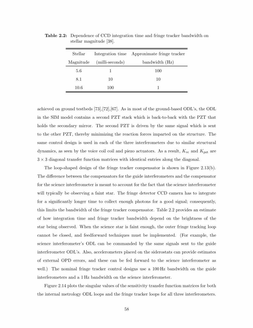
Table 2.2: Dependence of CCD integration time and fringe tracker bandwidth onstellar magnitude [38].

Stellar Integration time Approximate fringe tracker

Magnitude (milli-seconds) bandwidth (Hz)

5.6 1 100

8.1 10 10

10.6 100 1

achieved on ground testbeds [73],[72],[67]. As in most of the ground-based ODL’s, the ODL

in the SIM model contains a second PZT stack which is back-to-back with the PZT that

holds the secondary mirror. The second PZT is driven by the same signal which is sent

to the other PZT, thereby minimizing the reaction forces imparted on the structure. The

same control design is used in each of the three interferometers due to similar structural

dynamics, as seen by the voice coil coil and piezo actuators. As a result, Kvc and Kpzt are

3× 3 diagonal transfer function matrices with identical entries along the diagonal.

The loop-shaped design of the fringe tracker compensator is shown in Figure 2.13(b).

The difference between the compensators for the guide interferometers and the compensator

for the science interferometer is meant to account for the fact that the science interferometer

will typically be observing a faint star. The fringe detector CCD camera has to integrate

for a significantly longer time to collect enough photons for a good signal; consequently,

this limits the bandwidth of the fringe tracker compensator. Table 2.2 provides an estimate

of how integration time and fringe tracker bandwidth depend on the brightness of the

star being observed. When the science star is faint enough, the outer fringe tracking loop

cannot be closed, and feedforward techniques must be implemented. (For example, the

science interferometer’s ODL can be commanded by the same signals sent to the guide

interferometer ODL’s. Also, accelerometers placed on the siderostats can provide estimates

of external OPD errors, and these can be fed forward to the science interferometer as

well.) The nominal fringe tracker control designs use a 100 Hz bandwidth on the guide

interferometers and a 1 Hz bandwidth on the science interferometer.

Figure 2.14 plots the singular values of the sensitivity transfer function matrices for both

the internal metrology ODL loops and the fringe tracker loops for all three interferometers.

58

10−1

100

101

102

103

100

105

1010

Hz

Mag

nitu

de (

N/c

md)

Voice coil compensator

10−1

100

101

102

103

105

1010

Hz

Mag

nitu

de (

N/c

md)

PZT compensator

10−3

10−2

10−1

100

101

102

103

10−10

10−5

100

105

1010

Hz

Mag

nitu

de (

cmd/

m)

Fringe tracker compensator

Guide 1Guide 2Science

(a) (b)

Figure 2.13: (a) Transfer function magnitudes of voice coil controller Kvc (top)and PZT controller Kpzt (bottom). (b) Transfer function magni-tudes of fringe tracker controller.

The sensitivity transfer function matrix for a system with loop gain GK is defined as

(I + GK)−1, and large peaks in the maximum singular value of this function indicate

frequencies at which the system is sensitive to perturbations [28]. The sensitivity transfer

function is also good at indicating the frequency range over which the control is effective

in minimizing the effects of disturbances. Figure 2.14(a) shows that the ODL loops can

reject internal pathlength disturbances up to about 200 Hz. The fringe tracker sensitivity

in Figure 2.14(b) shows that the two guide interferometers (represented by the two smallest

singular values) have good disturbance rejection properties up to about 60 Hz, while the

science interferometer (associated with the largest singular value) is limited to about 7Hz

due to its lower bandwidth. The sensitivity transfer function does not provide an indication

of the stability of a system, so a Nyquist or a Nichols plot must be provided as well [28];

however, all controllers discussed in this section produce a stable system, and these plots

will be omitted.

A last control loop found within the integrated SIM model is the attitude control system.

The ACS loop shown in Figure 2.12(b) is in the form of a standard regulator, and the

control model simply assumes that the ACS compensator Kacs outputs desired moments

Mx, My, Mz based on a measure of the difference between the desired attitude and the actual

attitude. The compensator is in the form of a proportional-derivative (PD) controller with a

59

100

101

102

103

−140

−120

−100

−80

−60

−40

−20

0

20Singular values of ODL sensitivity transfer function

Frequency (Hz)

Mag

nitu

de (

dB)

σ1

σ2

σ3

10−2

10−1

100

101

102

103

−140

−120

−100

−80

−60

−40

−20

0

20Singular values of fringe tracker sensitivity transfer function

Frequency (Hz)

Mag

nitu

de (

dB)

σ1

σ2

σ3

(a) (b)

Figure 2.14: (a) Singular values of ODL sensitivity transfer function matrix. (b)Singular values of fringe tracker sensitivity transfer function matrix(with internal metrology loop closed).

highly-damped 2nd order lag filter to introduce a −20dB/decade roll-off at high frequencies.

The diagonal elements of the 3 × 3 compensator transfer function matrix are plotted in

Figure 2.15(a), and the slight difference in magnitude is due to non-identical spacecraft

mass moments of inertia about the principal axes. The corresponding singular value plot of

the sensitivity transfer function is shown in Figure 2.15(b), and it is evident that the ACS

loop has a bandwidth of approximately 0.1 Hz.

In the current SIM Classic model, no loops are closed between wavefront tilt measure-

ments and the fast-steering mirrors. If performance assessment does reveal that wavefront

tilt metrics exceed requirements, then these loops can be closed using compensators that

are of the same form as those used in ground-based experimental testbeds [70].

2.2.5 Reaction wheel assembly stochastic disturbance model

Now that the SIM integrated model has been described, the remaining task is to quan-

tify anticipated disturbances. One source of unwanted forces and moments on SIM and

other space-based observatories is the reaction wheel assembly (RWA). Reaction wheels can

impart disturbances at mid to high frequencies. The high frequencies can be beyond the

bandwidth of the optical control, thereby necessitating the use of some form of isolation.

Accurate reaction wheel disturbance models can lead to an increased level of confidence in

60

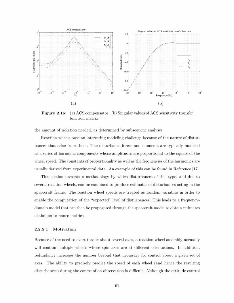
10−3

10−2

10−1

100

101

102

103

101

102

103

104

105

Hz

Mag

nitu

de (

N−

m/r

ad)

ACS compensator

Mx/θ

xM

y/θ

yM

z/θ

z

10−4

10−3

10−2

10−1

100

101

102

−100

−80

−60

−40

−20

0

20Singular values of ACS sensitivity transfer function

Frequency (Hz)

Mag

nitu

de (

dB)

σ1

σ2

σ3

(a) (b)

Figure 2.15: (a) ACS compensator. (b) Singular values of ACS sensitivity transferfunction matrix.

the amount of isolation needed, as determined by subsequent analyses.

Reaction wheels pose an interesting modeling challenge because of the nature of distur-

bances that arise from them. The disturbance forces and moments are typically modeled

as a series of harmonic components whose amplitudes are proportional to the square of the

wheel speed. The constants of proportionality as well as the frequencies of the harmonics are

usually derived from experimental data. An example of this can be found in Reference [17].

This section presents a methodology by which disturbances of this type, and due to

several reaction wheels, can be combined to produce estimates of disturbances acting in the

spacecraft frame. The reaction wheel speeds are treated as random variables in order to

enable the computation of the “expected” level of disturbances. This leads to a frequency-

domain model that can then be propagated through the spacecraft model to obtain estimates

of the performance metrics.

2.2.5.1 Motivation

Because of the need to exert torque about several axes, a reaction wheel assembly normally

will contain multiple wheels whose spin axes are at different orientations. In addition,

redundancy increases the number beyond that necessary for control about a given set of

axes. The ability to precisely predict the speed of each wheel (and hence the resulting

disturbances) during the course of an observation is difficult. Although the attitude control

61

logic that is used to issue commands to each wheel is known a priori, what is not known

to the the same level of certainty is the external torque disturbance which the wheels

are counteracting. Also, the initial wheel speeds at the start of an observation might be

impossible to predict. It is for these reasons that conducting a time simulation might not be

desirable. While initial conditions on wheel speeds can be assumed and external-torque time

histories can be estimated, the resulting simulation is valid only for that particular case.

What is more useful is a sense of how the performance metrics of interest (e.g., optical path

difference) are affected by disturbances arising from all possible combinations of wheel speed

variations. Running countless time simulations to try numerous combinations is prohibitive

due to the computational expense.

A possible alternative is to estimate what the disturbances are “on average.” These dis-

turbances can then be used in a first-cut performance assessment. If performance require-

ments are easily met even when appropriate bounds (e.g., 3σ) are placed on the outputs,

then the first-cut analysis might be all that is needed. If, however, the results of the analysis

are unclear as to whether the requirements can be satisfied, then a more refined approach

is necessary.

The “on-average” disturbance approach motivates the treatment of wheel speed as a

random variable. Making this assumption enables the mathematics of stochastic processes

to be applied in a systematic manner. Stochastic process theory is attractive because it per-

mits a random process to be described in the frequency domain by a power spectral density

(PSD) function. This can then be used in a frequency-domain disturbance analysis, which

can be less computationally intensive that a time-domain simulation. Another advantage

to the “on-average” approach is that external torque models and initial wheel speeds are

not required.

The following analysis is somewhat analogous to the derivation by Melody in [60].

Melody treats the wheel speed as a random variable and proceeds to derive expressions

for the PSD’s of axial force, radial force, and radial torque for a single wheel. The objective

of the current work is to follow a similar approach, but to consider the general case of

multiple wheels at specified orientations with respect to the spacecraft axes.

62

2.2.5.2 Disturbance Model and Nomenclature

We begin by defining a reaction wheel disturbance model consisting of a series of harmonic

components of the form

mijk(t) = Cjkf2i sin(2πhjkfit+ φijk) (2.19)

where

m = disturbance force (j = 1, 2, 3) or torque (j = 4, 5, 6)

i = wheel number (1, 2, . . . , N); N = total number of wheels

j = disturbance number (1, 2, . . . , 6); (see Eq. 2.21)

k = harmonic number (1, 2, . . . , nj); nj = number of

harmonics for jth disturbance number

Cjk = amplitude coefficient for kth harmonic of jth

disturbance; assumed the same for all wheels

fi = wheel speed of ith wheel (in Hz)

hjk = ratio of frequency of kth harmonic of jth disturbance

to frequency of wheel rotation; assumed the same for all wheels

φijk = phase angle of kth harmonic of jth disturbance of ith wheel

Both fi and φijk are assumed to be independent random variables. By independent we

mean that the joint probability density function (PDF) can be written as the product of the

individual PDF’s. If we use the notation fX(x) to denote the PDF of the random variable

X, then independence implies fHjkΦijk(hjk, φijk) = fHjk

(hjk)fΦijk(φijk).

The total disturbance of type j for the ith wheel is simply the sum over the harmonics.

mij(t) =nj∑

k=1

mijk(t) (2.20)

Let us now define the disturbances in the local coordinate frame of a wheel. The pre-

63

x

y

zw

w

w

Figure 2.16: Local wheel frame (z axis along spin axis, x axis and y axis in planeof wheel).

superscript w signifies that the disturbances are expressed in the wheel frame.

wmi(t) =

w

m1(t)

m2(t)

m3(t)

m4(t)

m5(t)

m6(t)

i

=

w

Fx(t)

Fy(t)

Fz(t)

Mx(t)

My(t)

Mz(t)

i

(2.21)

The local wheel axes are shown in Figure 2.16. These axes remain fixed in space and do not

rotate as the wheel spins. Fx and Fy are the radial forces, Fz is the axial force, Mx and My

are the torques about orthogonal radial axes, and Mz is the torque about the wheel’s spin

axis. One simplification that can be made (and which is supported by experimental data) is

that Mz is approximately zero. For instance, the causes that contribute to Mz (torque ripple

and motor cogging) were found to be negligible for the Hubble Space Telescope reaction

wheels [60]. Recall however that the torque required for attitude control is provided by Mz.

This torque will not be included in the disturbance model since it is assumed that it will

be accounted for in the ACS loop of the closed-loop spacecraft model.

The radial disturbances are assumed to rotate in the plane of the wheel at the frequencies

of the harmonics. Hence, the disturbance forces in, and the moments about, the y axis are

90 out of phase with the disturbance forces in, and moments about, the x axis. This

suggests that the following relationship holds:

φijk = φi(j−1)k +π

2, j = 2, 5 (2.22)

64

2.2.5.3 Transformation of Disturbances

The transformation of the disturbances from the local wheel frame to the global spacecraft

frame requires a rotation matrix. The orientation of the wheel frame relative to the space-

craft frame can be specified by a set of Euler angles. Define the so-called XY Z Euler angles

as follows. Begin by having the local wheel axes aligned with the spacecraft axes1. Each of

the three Euler angles specifies rotation about an intermediate axis. In particular, let

β = angle of rotation about original z axis

θ = angle of rotation about new y axis after previous rotation

γ = angle of rotation about new x axis after previous rotation

These rotations are shown in Figure 2.17.

oyw

oz w

ox w

xs/c

ys/c

zs/c

ox w

oyw

x w/ x w

/

oz w

z w//

z w//

yw/

yw/

x w//

β

z w/,

θ

first rotation second rotation

, yw//

x w,

, ywyw///,z w z w

///

third rotation

γ

Figure 2.17: XY Z Euler angles (xw, yw, and zw are axes of actual wheel frame).

Let

s/cp be a vector in the spacecraft axeswp be a vector in the wheel axes

Ri be the 3× 3 rotation matrix from the ith wheel frame to the spacecraft frame.

Then s/cp = Riwp, and it can be shown that Ri is of the form

Ri =

cβicθi cβisθisγi − sβicγi cβisθicγi + sβisγi

sβicθi sβisθisγi + cβicγi sβisθicγi − cβisγi

−sθi cθisγi cθicγi

(2.23)

1Note: The “spacecraft” axes might not be the same as the global axes (e.g., the coordinate frame used

to build the finite-element model). In this thesis, the spacecraft axes will refer to the coordinate frame whose

origin is at the location at which the disturbance forces and moments are desired. In most cases, this frame

will be parallel to but displaced from the global frame.

65

where “c” is an abbreviation for “cos” and “s” is an abbreviation for “sin”.

The axes now need to be displaced to account for the fact that all the wheels are not at

the same location. A simplifying assumption is that the spin axis (z axis) of all the wheels

intersect at a point, which happens to coincide with the origin of the spacecraft axes. Let

the distance from this point to each of the wheel frame origins be d. Then the vector from

the spacecraft frame origin to the origin of the ith wheel frame is given by

s/cri = Riwri = Ri

0

0

d

(2.24)

and is shown graphically in Figure 2.18.

z w

xs/c

ys/c

zs/c

r

O

Figure 2.18: Position vector r, which locates the wheel frame origin in the space-craft frame.

The moment about O (in the spacecraft frame) due to the forces Fx, Fy, Fz in the wheel

frame is given by the cross product

s/cri ×

Ri

wFx

Fy

Fz

i

We can now express in the spacecraft frame the disturbance forces and moments due to

a single wheel. The disturbances can be written in terms of the rotation matrix Ri, the

moment arms ri, and local disturbances wmi. As a means of simplification, the cross

66

product r× ( ) can be written as a matrix multiplication as follows

ri × a =

0 −r3 r2

r3 0 −r1−r2 r1 0

i︸ ︷︷ ︸≡Ri

a (2.25)

The disturbance vector in the spacecraft frame is therefore

s/cmi(t) =

Ri 03×3

ri × (Ri Ri

wmi(t) =

Ri 03×3

RiRi Ri

︸ ︷︷ ︸call this Ti

wmi(t) = Tiwmi(t) (2.26)

The individual wheel disturbances can then be summed to obtain the overall disturbance

acting in the spacecraft frame.

s/cm(t) =N∑

i=1

s/cmi(t) =

s/c

m1(t)

m2(t)

m3(t)

m4(t)

m5(t)

m6(t)

=

s/c

Fx(t)

Fy(t)

Fz(t)

Mx(t)

My(t)

Mz(t)

(2.27)

2.2.5.4 Calculation of the Spectral Density Matrix

The objective now is to derive the spectral density matrix of s/cm(t). The first step is to

determine the correlation matrix, Rs/cm(t1, t2). Let E[(·)] signify the expectation operator.

Rs/cm(t1, t2) = E[s/cm(t1)s/cmT (t2)

](2.28)

= E

N∑

p=1

s/cmp(t1)

N∑

q=1

s/cmTq (t2)

(2.29)

Now substitute the transformation s/cmi(t) = Tiwmi(t) (which was defined in Eq. 2.26).

Rs/cm(t1, t2) = E

N∑

p=1

Tpwmp(t1)

N∑

q=1

wmTq (t2)T T

q

(2.30)

= E

N∑

p=1

N∑q=1

Tpwmp(t1)wmT

q (t2)T Tq

67

Neither Tp nor Tq is a function of a random variable, so the expectation operator can be

brought inside the summation.

Rs/cm(t1, t2) =N∑

p=1

N∑q=1

TpE[wmp(t1)wmT

q (t2)]

︸ ︷︷ ︸=Rwmpwmq (t1,t2)

T Tq (2.31)

=N∑

p=1

N∑q=1

Tp

...

· · · Rwmprwmqs(t1, t2) · · ·

...

T T

q

Thus, the correlation matrix of s/cm can be written in terms of the transformation matrices

Tp and Tq and the cross-correlation matrix of wmp and wmq, where p and q loop over the

number of wheels.

As shown in Eq. 2.31, scalar cross-correlation terms like Rwmprwmqs(t1, t2) appear. Ex-

panding this term using Eq. 2.19 and Eq. 2.20,

Rwmprwmqs(t1, t2)

= E [mpr(t1)mqs(t2)] (2.32)

= E

[nr∑

k=1

Crkf2p sin(2πhrkfpt1 + φprk)

ns∑l=1

Cslf2q sin(2πhslfqt2 + φqsl)

]

= E

[nr∑

k=1

ns∑l=1

CrkCslf2pf

2q sin(2πhrkfpt1 + φprk)sin(2πhslfqt2 + φqsl)

]

Making use of the trigonometric identity sinAsinB = 12 [cos(A−B)− cos(A+B)] leads to

Rwmprwmqs(t1, t2) = E

[nr∑

k=1

ns∑l=1

CrkCslf2p f

2q

2cos (2π(hrkfpt1 − hslfqt2) + φprk − φqsl) (2.33)

− cos (2π(hrkfpt1 + hslfqt2) + φprk + φqsl)]

The random variables are fp, fq, φprk, and φqsl. We make the following assumptions:

• φ’s are independent (except when Eq. 2.22 is in effect)

• φ’s are uniform random variables over the interval [0, 2π]

• f ’s are independent, and the probability density function of the pth wheel is expressed

as fFP(fp)

We now consider several cases.

68

Case 1

p = q and r = s (i.e., same wheel and same disturbance number)

This case is identical to that considered by Melody in [60]. The result is equivalent to

Rwmprwmpr(t1, t2) =

nr∑k=1

C2rk

2E[f4

p cos (2πhrkfp(t1 − t2))]

(2.34)

Letting t1 − t2 = τ leads to the following stationary autocorrelation function.

Rwmprwmpr (τ) =

nr∑k=1

C2rk

2E[f4

p cos (2πhrkfpτ)]

(2.35)

Case 2

p = q and (r, s) ∈ [(1, 2), (2, 1), (4, 5), (5, 4)] (i.e., same wheel, and disturbances are of the

same type and 90 out of phase)

Appendix B derives the result

Rwmprwmps(τ) = ∓

nr∑k=1

C2rk

2E[f4

p sin (2πhrkfpτ)],

− , r > s

+ , r < s(2.36)

Case 3

p = q and (r, s) 6∈ [(1, 2), (2, 1), (4, 5), (5, 4)] and r 6= s (i.e., remaining combinations of r

and s for the same wheel)

Using the definition of the expectation operator to rewrite Eq. 2.33 produces

Rwmprwmps(t1, t2) =

nr∑k=1

ns∑l=1

∫ +∞

−∞

∫ 2π

0

∫ 2π

0

CrkCslf4p

2cos [2πfp(hrkt1 − hslt2) + φprk − φpsl]

(2.37)

− cos [2πfp(hrkt1 + hslt2) + φprk + φpsl] 12π

12π

fFP(fp)dφprkdφpsldfp = 0

The entire expression is equal to zero because φprk and φpsl are uniformly distributed over

[0, 2π] and are independent. To see this, consider the following simplified case.∫ 2π

0cos(φ+A)dφ = 0 (2.38)

Integrating a cosine function over one period will always produce zero. So for every cosine

term that contains a φprk or φpsl, the integral from 0 to 2π with respect to φprk or φpsl will

vanish.

69

Case 4

p 6= q (i.e., different wheels and any combination of disturbances)

Allowing different wheel speeds still produces the same result.

Rwmprwmqs(t1, t2) =

nr∑k=1

ns∑l=1

∫ +∞

−∞

∫ 2π

0

∫ 2π

0

CrkCslf2pf

2q

2cos (2π(hrkfpt1 − hslfqt2) + φprk − φqsl)

(2.39)

− cos (2π(hrkfpt1 + fqhslt2) + φprk + φqsl) 12π

12π

fFP(fp)fFQ

(fq)dφprkdφqsldfqdfp = 0

since φprk and φqsl are uniformly distributed over [0, 2π] and are independent.

At this point, all the various correlation functions have been computed. The next step

is to derive the spectral density functions. Taking the Fourier transform of Eq. 2.31 (which

can be done since all the nonzero correlation functions have been shown to be functions of

a single time-lag variable τ) results in

Ss/cm(ω) =N∑

p=1

N∑q=1

Tp

...

· · · Swmprwmqs(ω) · · ·...

T T

q (2.40)

where Ss/cm(ω) signifies the spectral density matrix of the reaction wheel disturbances in

the spacecraft frame.

The spectral density functions corresponding to each of the four cases can now be

determined.

Case 1

p = q and r = s

As before, this case was considered by Melody in [60]. The resulting PSD is given by

Swmprwmpr(ω) =

nr∑k=1

πC2rkω

4

2(2πhrk)5

[fFP

(ω

2πhrk

)+ fFP

( −ω2πhrk

)](2.41)

Case 2

p = q and (r, s) ∈ [(1, 2), (2, 1), (4, 5), (5, 4)]

70

Appendix B derives the following result.

Swmprwmps(ω) = ±

nr∑k=1

jπC2rkω

4

2(2πhrk)5

[fFP

(ω

2πhrk

)+ fFP

( −ω2πhrk

)],

+ , r > s

− , r < s

j =√−1

(2.42)

Note that this only differs from the result of the p = q and r = s case by a factor of ±j.

Case 3 and Case 4

These cases lead to the result Swmprwmqs(ω) = 0 since the corresponding correlation func-

tions are zero.

The double sum in Eq. 2.40 can be replaced by a single sum since all the terms in which

p 6= q drop out.

Ss/cm(ω) =N∑

p=1

Tp

...

· · · Swmprwmps(ω) · · ·...

T T

p =N∑

p=1

TpSwmp(ω)T Tp (2.43)

If we make the further assumption that all the wheels have the same wheel speed probability

density function, namely fF1(f1) = fF2(f2) = · · · = fFN(fN ), as well as the same amplitude

coefficients and harmonics, then we obtain

Ss/cm(ω) =N∑

p=1

Tp

...

· · · Swmprwmps(ω) · · ·...

T T

p (2.44)

=N∑

p=1

Tp

Sm1(ω) Sm1m2(ω)

Sm2m1(ω) Sm2(ω)

Sm3(ω)

Sm4(ω) Sm4m5(ω)

Sm5m4(ω) Sm5(ω)

Sm6(ω)

T T

p

and elements not shown are equal to zero. For simplicity we use the notation Smj(ω)

to represent the PSD of the jth disturbance of a single wheel in local wheel coordinates.

71

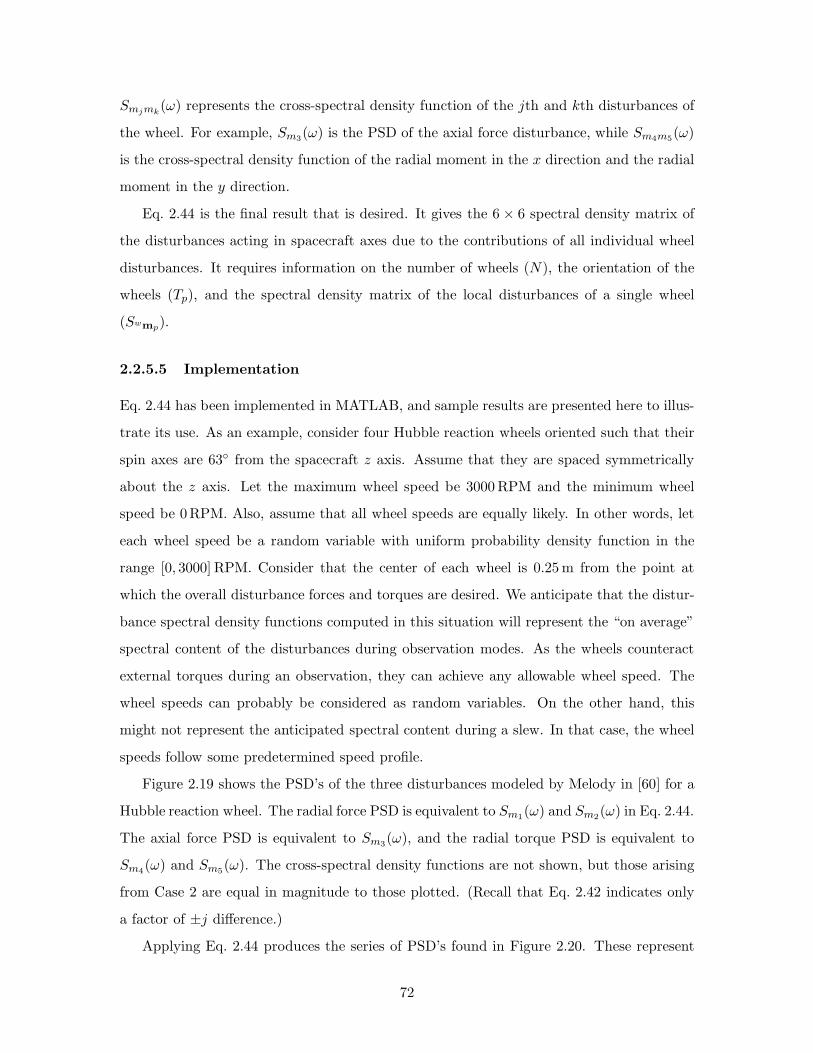
Smjmk(ω) represents the cross-spectral density function of the jth and kth disturbances of

the wheel. For example, Sm3(ω) is the PSD of the axial force disturbance, while Sm4m5(ω)

is the cross-spectral density function of the radial moment in the x direction and the radial

moment in the y direction.

Eq. 2.44 is the final result that is desired. It gives the 6 × 6 spectral density matrix of

the disturbances acting in spacecraft axes due to the contributions of all individual wheel

disturbances. It requires information on the number of wheels (N), the orientation of the

wheels (Tp), and the spectral density matrix of the local disturbances of a single wheel

(Swmp).

2.2.5.5 Implementation

Eq. 2.44 has been implemented in MATLAB, and sample results are presented here to illus-

trate its use. As an example, consider four Hubble reaction wheels oriented such that their

spin axes are 63 from the spacecraft z axis. Assume that they are spaced symmetrically

about the z axis. Let the maximum wheel speed be 3000 RPM and the minimum wheel

speed be 0RPM. Also, assume that all wheel speeds are equally likely. In other words, let

each wheel speed be a random variable with uniform probability density function in the

range [0, 3000] RPM. Consider that the center of each wheel is 0.25 m from the point at

which the overall disturbance forces and torques are desired. We anticipate that the distur-

bance spectral density functions computed in this situation will represent the “on average”

spectral content of the disturbances during observation modes. As the wheels counteract

external torques during an observation, they can achieve any allowable wheel speed. The

wheel speeds can probably be considered as random variables. On the other hand, this

might not represent the anticipated spectral content during a slew. In that case, the wheel

speeds follow some predetermined speed profile.

Figure 2.19 shows the PSD’s of the three disturbances modeled by Melody in [60] for a

Hubble reaction wheel. The radial force PSD is equivalent to Sm1(ω) and Sm2(ω) in Eq. 2.44.

The axial force PSD is equivalent to Sm3(ω), and the radial torque PSD is equivalent to

Sm4(ω) and Sm5(ω). The cross-spectral density functions are not shown, but those arising

from Case 2 are equal in magnitude to those plotted. (Recall that Eq. 2.42 indicates only

a factor of ±j difference.)

Applying Eq. 2.44 produces the series of PSD’s found in Figure 2.20. These represent

72

100

101

102

103

10−10

10−9

10−8

10−7

10−6

10−5

10−4

10−3

10−2

Frequency (Hz)

Mag

nitu

de

Power Spectral Density Functions

radial force PSD [N2/Hz] axial force PSD [N2/Hz] radial torque PSD [(Nm)2/Hz]

Figure 2.19: Power spectral density functions of disturbances from a Hubble-classreaction wheel with uniform probability density function in the in-terval [0, 3000]RPM. Based on the disturbance model from Melody[60].

the diagonal elements of Ss/cm(ω). Due to the symmetry of the problem, the Fx and Fy

PSD’s overlap, as do the Mx and My PSD’s.

The off-diagonal elements (i.e., cross-spectral density functions) are not all zero, as

indicated in Figure 2.21. A representative subset of these functions is plotted. Since cross-

spectral density functions are typically complex-valued, both the magnitude and phase are

shown. Note that the phase corresponding to the larger magnitude functions is ±90, which

indicates a factor of ±j. The phase corresponding to the smaller magnitude functions is

corrupted by numerical noise.

2.2.5.6 Comments

Because the wheel speeds and phase angles of the harmonics are treated as independent

random variables, the disturbance spectral densities can be thought of as the “expected”

levels. What this approach probably does not capture is the worst-case disturbance level.

Lifting some of the assumptions on independence might lead to a better approximation of the

73

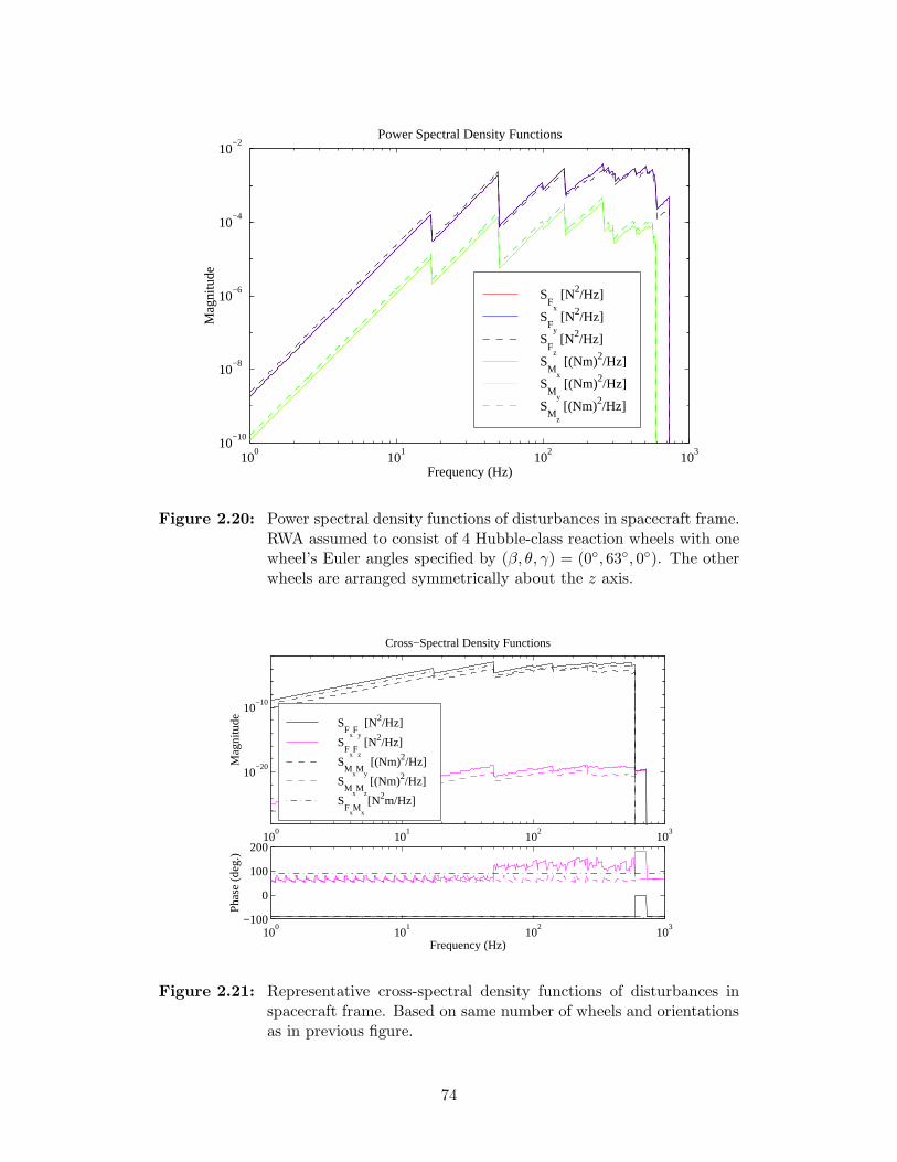
100

101

102

103

10−10

10−8

10−6

10−4

10−2

Frequency (Hz)

Mag

nitu

de

Power Spectral Density Functions

SF

x

[N2/Hz]

SF

y

[N2/Hz]

SF

z

[N2/Hz]

SM

x

[(Nm)2/Hz]

SM

y

[(Nm)2/Hz]

SM

z

[(Nm)2/Hz]

Figure 2.20: Power spectral density functions of disturbances in spacecraft frame.RWA assumed to consist of 4 Hubble-class reaction wheels with onewheel’s Euler angles specified by (β, θ, γ) = (0, 63, 0). The otherwheels are arranged symmetrically about the z axis.

100

101

102

103

10−20

10−10

Mag

nitu

de

Cross−Spectral Density Functions

SF

xF

y

[N2/Hz]

SF

xF

z

[N2/Hz]

SM

xM

y

[(Nm)2/Hz]

SM

xM

z

[(Nm)2/Hz]

SF

xM

x

[N2m/Hz]

100

101

102

103

−100

0

100

200

Frequency (Hz)

Pha

se (

deg.

)

Figure 2.21: Representative cross-spectral density functions of disturbances inspacecraft frame. Based on same number of wheels and orientationsas in previous figure.

74

worst case. For instance, Eq. 2.33 can be used as the starting point, and new assumptions

such as that all wheels are at the same speed (i.e., fp = fq = f) and all disturbances

are at the same “clock angle” (i.e., φprk, φqsl → φrk, φrk) can be made. Following the

same procedure as has been outlined previously will lead to a different expression for the

total disturbance spectral density matrix than what is shown in Eq. 2.44. The assumption

of equivalent wheel speeds is valid when wheel speeds “cross” as angular momentum is

transferred from one wheel to another. Further analysis is required to determine how well

the frequency-domain approach can predict the effects of these scenarios.

Another issue not brought up in this section but which is of concern is how resonances

of the reaction wheel and/or the test mount affect the PSD’s. Reference [17] clearly shows

a case where the mount resonance at approximately 100 Hz is visible in a waterfall plot

from a test of a single Hubble reaction wheel. Reference [6] describes some internal wheel

modes that can occur below 100 Hz. Figure 2.20 indicates a large amount of energy above

100 Hz. It might be unlikely that this energy will be unattenuated before it propagates

into the spacecraft. A possible remedy is to create a physical model which includes the

effects of wheel resonances and mount dynamics. If the true disturbance sources can be

identified from the test data, then they can be used to drive the physical model which has

been coupled to the spacecraft model. This should provide the most accurate results, but

it is unclear whether the complexity of this approach will outweigh any improved accuracy.

One last issue deals with how appropriate it is to use reaction wheel disturbance models

derived from “blocked-force” tests (i.e., tests conducted when the wheel is mounted to a

rigid base). The impedance of the spacecraft at the location of the RWA will be different

from that which the wheel sees during the test. Consequently, the actual disturbances

entering the spacecraft might not be the same as what is modeled. It is recommended that

more work in this area be conducted to see if a truly coupled model is required.

2.3 Summary

This chapter has provided an overview of the integrated modeling process. This process

unifies structural, control, performance, and disturbance models into an overall disturbance-

to-performance model required for performance assessment. To help illustrate this, the

Space Interferometry Mission has been described and has served as an example of a high

75

performance optical system. The structural, control, and optical models were described in

some detail so that the results of analyses in later chapters can be better understood.

In addition, a general methodology has been developed which uses individual reaction

wheel stochastic disturbance models to produce the total spectral density function matrix

of the disturbances in the spacecraft frame. The spectral density function matrix for the

disturbances of a single wheel is first derived in the local wheel frame. This is based on

a harmonic disturbance model which treats the wheel speed and phase angles as random

variables. This work extends the results presented by Melody in [60] by also deriving the

cross-spectral density functions. A coordinate transformation is then applied to express the

disturbances in the spacecraft frame, and the contributions from all the wheels are summed.

This then facilitates their use in subsequent disturbance analyses.

76

Chapter 3

Disturbance Analysis Framework

After developing an integrated model of a nominal system design, as described in the

previous chapter, the next step is to assess the performance when the model is subjected to

anticipated disturbances. Disturbance analyses are usually conducted in order to predict

the effect of disturbances on system outputs of interest. The disturbances can be modeled in

a number of forms, and as a result, various types of disturbance analyses can be performed.

This chapter summarizes three particular types of disturbance analyses and illustrates the

use of a MATLAB code that was developed to implement each one.

3.1 Types of Disturbance Analyses

There are at least three ways in which a disturbance analysis can be conducted on the

nominal plant model. The approaches include:

• time domain

• frequency domain

• Lyapunov

This section will introduce each one and then demonstrate their use on a simple single

degree-of-freedom system. Practical issues related to the accuracy of the results will be

discussed. Section 3.3 will show sample results of a frequency-domain analysis on a model

of the Space Interferometry Mission (SIM).

77

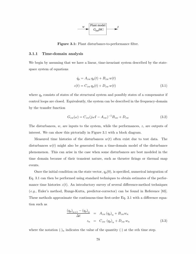
Gzw(ω)Plant modelw z

Figure 3.1: Plant disturbance-to-performance filter.

3.1.1 Time-domain analysis

We begin by assuming that we have a linear, time-invariant system described by the state-

space system of equations

qp = Azw qp(t) +Bzw w(t)

z(t) = Czw qp(t) +Dzw w(t) (3.1)

where qp consists of states of the structural system and possibly states of a compensator if

control loops are closed. Equivalently, the system can be described in the frequency-domain

by the transfer function

Gzw(ω) = Czw(jωI −Azw)−1Bzw +Dzw (3.2)

The disturbances, w, are inputs to the system, while the performances, z, are outputs of

interest. We can show this pictorially in Figure 3.1 with a block diagram.

Measured time histories of the disturbances w(t) often exist due to test data. The

disturbances w(t) might also be generated from a time-domain model of the disturbance

phenomenon. This can arise in the case when some disturbances are best modeled in the

time domain because of their transient nature, such as thruster firings or thermal snap

events.

Once the initial condition on the state vector, qp(0), is specified, numerical integration of

Eq. 3.1 can then be performed using standard techniques to obtain estimates of the perfor-

mance time histories z(t). An introductory survey of several difference-method techniques

(e.g., Euler’s method, Runge-Kutta, predictor-corrector) can be found in Reference [83].

These methods approximate the continuous-time first-order Eq. 3.1 with a difference equa-

tion such as

(qp)n+1 − (qp)n

∆t= Azw (qp)n +Bzwwn

zn = Czw (qp)n +Dzw wn (3.3)

where the notation (·)n indicates the value of the quantity (·) at the nth time step.

78

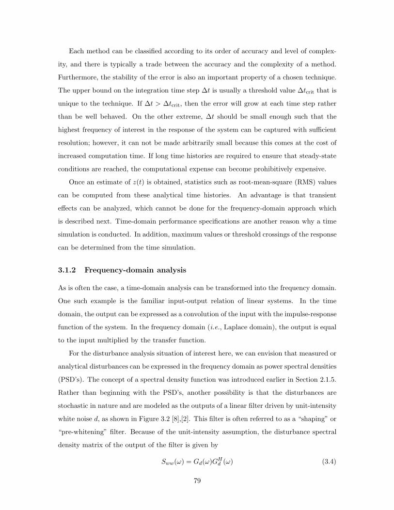
Each method can be classified according to its order of accuracy and level of complex-

ity, and there is typically a trade between the accuracy and the complexity of a method.

Furthermore, the stability of the error is also an important property of a chosen technique.

The upper bound on the integration time step ∆t is usually a threshold value ∆tcrit that is

unique to the technique. If ∆t > ∆tcrit, then the error will grow at each time step rather

than be well behaved. On the other extreme, ∆t should be small enough such that the

highest frequency of interest in the response of the system can be captured with sufficient

resolution; however, it can not be made arbitrarily small because this comes at the cost of

increased computation time. If long time histories are required to ensure that steady-state

conditions are reached, the computational expense can become prohibitively expensive.

Once an estimate of z(t) is obtained, statistics such as root-mean-square (RMS) values

can be computed from these analytical time histories. An advantage is that transient

effects can be analyzed, which cannot be done for the frequency-domain approach which

is described next. Time-domain performance specifications are another reason why a time

simulation is conducted. In addition, maximum values or threshold crossings of the response

can be determined from the time simulation.

3.1.2 Frequency-domain analysis

As is often the case, a time-domain analysis can be transformed into the frequency domain.

One such example is the familiar input-output relation of linear systems. In the time

domain, the output can be expressed as a convolution of the input with the impulse-response

function of the system. In the frequency domain (i.e., Laplace domain), the output is equal

to the input multiplied by the transfer function.

For the disturbance analysis situation of interest here, we can envision that measured or

analytical disturbances can be expressed in the frequency domain as power spectral densities

(PSD’s). The concept of a spectral density function was introduced earlier in Section 2.1.5.

Rather than beginning with the PSD’s, another possibility is that the disturbances are

stochastic in nature and are modeled as the outputs of a linear filter driven by unit-intensity

white noise d, as shown in Figure 3.2 [8],[2]. This filter is often referred to as a “shaping” or

“pre-whitening” filter. Because of the unit-intensity assumption, the disturbance spectral

density matrix of the output of the filter is given by

Sww(ω) = Gd(ω)GHd (ω) (3.4)

79

Gzw(ω)Gd(ω)Plant modelDisturbance model

white noise

d w z

Figure 3.2: Disturbance filter and plant disturbance-to-performance filter.

Thus, Sww(ω) can be specified directly or can be obtained from a shaping filter model.

In either case, given the disturbance spectral density matrix Sww(ω) and the transfer

function matrix Gzw(ω), the performance spectral density matrix can be computed from

the relation (see [86])

Szz(ω) = Gzw(ω)Sww(ω)GHzw(ω) (3.5)

This can also be expressed in the more typical frequency units of Hz.

Szz(f) = Gzw(f)Sww(f)GHzw(f) (3.6)

Sww(ω) can be a continuous function of frequency, or for the case of disturbances consisting

of a series of discrete harmonics, it can contain impulses at the frequencies of the harmonics.

In the latter case, Szz(ω) will also contain a series of impulses.

Szz(ω) provides information on the frequency content of the performance metrics. As

shown previously in Eq. 2.11, integrating the elements of a spectral density function matrix

across frequency and scaling by 12π (if the frequency is in rad/s) yields the covariance matrix

(for zero-mean processes).

Σz =12π

∫ +∞

−∞Szz(ω) dω

=∫ +∞

−∞Szz(f) df (3.7)

The variance of the ith performance metric is therefore given by

σ2zi

= [Σz]i,i =12π

∫ +∞

−∞[Szz(ω)]i,i dω

=∫ +∞

−∞[Szz(f)]i,i df

= 2∫ +∞

0[Szz(f)]i,i df (3.8)

Taking the square root of σ2zi

produces the root-mean-square (RMS) value. This is conve-

nient since in many instances requirements are placed on RMS values of the performance

metrics. The quantity 2 [Szz(f)]i,i will be referred to as a one-sided PSD.

80

Although Eq. 3.8 provides an attractive way to determine the mean-square value of the

performance, there are some practical issues that can affect the accuracy of the results.

The first issue arises when the disturbance spectral density matrix is either measured ex-

perimentally or generated analytically and is passed on to the person who will conduct the

disturbance analysis. An incorrect assumption might be made regarding the form of the

PSD’s (e.g., rad/s vs. Hz, one-sided vs. two-sided). It is therefore extremely important that

there are no misunderstandings if such a hand-off occurs.

Two other issues deal with numerical integration. The df in Eq. 3.8 is replaced by

the frequency resolution ∆f . Too large of a ∆f can cause important narrowband features

(e.g., lightly-damped modes) to be missed. This can result in an incorrect RMS estimate,

so it is important that additional frequency points be added around each mode and at the

frequency of each mode (where the peak occurs). The appropriate number is directly related

to the damping and frequency of each mode since a mode’s “bandwidth” is proportional to

the quantity ζω. The number to add is also dependent on how strongly each mode appears

in the outputs of interest. For example, there is no need to increase the frequency resolution

around a mode that is completely unobservable or undisturbable. Rather than stating any

rules of thumb, it is recommended that a cumulative RMS plot (which is discussed shortly)

be inspected to determine if the frequency resolution is sufficient.

The limits of integration usually span a finite frequency range when a numerical inte-

gration scheme such as trapezoidal integration is used. (The frequency limits might also be

set by the frequency range of a measured PSD.) This results in Eq. 3.8 being expressed in

terms of the minimum and maximum frequencies, fmin and fmax.

σ2zi≈ 2

∫ +fmax

−fmin

[Szz(f)]i,i df (3.9)

It is important to ensure that the frequency range that contributes most to the RMS value is

sufficiently captured within these limits. This also impacts model reduction since important

modes within the range should be retained. One way to check this is by computing the

cumulative RMS function.

81

Cumulative RMS and cumulative variance functions

Define a cumulative RMS function σzi,c(fo) as

σzi,c(fo) =

(2∫ +fo

−fmin

[Szz(f)]i,i df

) 12

(3.10)

where fo ∈ [ fmin . . . fmax ]. If most of the energy lies within this range, then σzi,c(fmax)

should be very close to the true value σzi . An indication that the frequency range might

not be sufficient is if the cumulative RMS curve has a significant slope (when plotted on

a linear vertical scale) near either fmin or fmax. This would suggest that frequencies just

below or just above the range would contribute a non-negligible amount. Consequently, one

clue that the frequency range is sufficient is if it appears as if the cumulative RMS curve is

asymptotically approaching a horizontal line near the frequency limits.

It should be pointed out, however, that even if the cumulative RMS has this feature,

it still does not ensure a correct overall RMS value. Lightly-damped modes that are well

outside the bandwidth can still contribute a significant amount of energy. To avoid this situ-

ation, the PSD should roll off at a rate such that an unmodelled mode at higher frequencies

would still not be able to contribute significantly to the RMS.

Besides indicating if the frequency range of integration is sufficient, a cumulative RMS

curve can also help to identify the frequencies of critical structural modes in the system. The

important modes are often those that are lightly damped, and these manifest themselves as

sharp “steps” in a cumulative RMS curve. To notice why this is the case, first differentiate

the square of Eq. 3.10 with respect to fo.

dσ2zi,c(fo)dfo

=d

dfo

(2∫ +fo

−fmin

[Szz(f)]i,i df

)

= 2Szz(fo) (3.11)

The function σ2zi,c(fo) is the cumulative variance, and its slope at a particular frequency

is simply twice the value of the PSD at that frequency. So if fo is in the vicinity of a

lightly-damped mode, [Szz(f)]i,i will be large, thereby implying that the slope will be steep.

[Szz(f)]i,i is also always a positive and real function since it is a PSD; consequently, the

cumulative variance is a non-decreasing function.

Another use of the cumulative variance plot is to determine if there are enough frequency

points around the critical modes. If the locations of frequency points are indicated on the

82

plot, then the “density” of points within each step can be examined. A sharp step that

is comprised of only a few points is an indication that the frequency resolution is not

sufficient. Since the cumulative variance (area) rapidly changes in the vicinity of a mode, a

more accurate estimate requires enough points to capture this rate of change.

The cumulative variance can also provide a quick indication of the percent contribution

of each of the lightly-damped modes. First define a normalized cumulative variance function

that has a maximum value of 1.

σ2zi,c(fo) ≡

σ2zi,c(fo)

σ2zi,c(fmax)

(3.12)

When a sharp step is present in a plot of σ2zi,c(fo) due to a mode, that mode’s contribution

can be approximated as the “height” of the step. For example, if the step begins at a value

of 0.2 and ends at a value of 0.9, then the mode responsible for that step can be thought

of as contributing about 70% to the overall variance. This is not as simple to do when

there are closely-spaced modes; however, the plot still can indicate the contributions from

all modes in a certain frequency range.

Since a cumulative RMS function and the associated cumulative variance function con-

tain useful information, it is recommended that either one of them always be plotted with

the corresponding PSD. It is for this reason that most of the PSD plots in this thesis have

a cumulative RMS subplot above them.

Disturbance contributions

While the cumulative RMS function indicates critical modes, what is also important is iden-

tifying which disturbances excite the critical modes the most. To help with this, disturbance

contributions can be calculated.

For the special case when all the disturbances are uncorrelated, the spectral density

matrix Sww(ω) will be a diagonal matrix. Eq. 3.5 can then be simplified to

Szkzk(ω) =

# of dist.∑i=1

|Gzkwi(jω)|2Swiwi(ω)︸ ︷︷ ︸≡S(zkzk)i

(ω)

(3.13)

where Szkzk(ω) is the PSD of the kth performance metric, Swiwi(ω) is the PSD of the ith

disturbance, and Gzkwi(jω) is the transfer function from the ith disturbance to the kth

performance. These are all scalar functions of frequency. The notation S(zkzk)iis used to

83

represent the contribution of the ith disturbance to the kth performance. Eq. 3.13 indicates

that the overall performance PSD can be though of as a sum of PSD’s due to each of

the separate disturbances. At a particular frequency, the percent contribution of the ith

disturbance can be calculated to be

% contribution =S(zkzk)i

(ω)Szkzk

(ω)× 100% (3.14)

This value can also be plotted as a function of frequency for each of the performance metrics.

Near the frequencies of the critical modes, the plot can help identify which disturbances

are exciting the important modes the most. If the disturbances are correlated, then a

disturbance contribution approximation can be made which ignores the off-diagonal terms

in Sww(ω).

Summary of frequency-domain analysis steps

Generally, the frequency-domain approach is more efficient than a time-domain analysis.

The most computationally-intensive task that is required is evaluating the transfer function

matrix. After that, only matrix multiplications and numerical integration (e.g., trapezoidal

integration) is necessary. The key computation steps involve:

• Determining the transfer function matrix Gzw(ω) from Eq. 3.2. (If Azw is fairly large,

a brute force inversion of jωI − Azw would be impractical. A state transformation

that produces a diagonal Azw would lead to a more efficient computation.)

• Performing the matrix multiplication in Eq. 3.6 at each frequency.

• Numerically integrating the PSD’s (Eq. 3.9).

• Calculating the cumulative RMS and/or variance curves from Eq. 3.10 and Eq. 3.12.

• Calculating the disturbance contributions using Eq. 3.13 and Eq. 3.14 (for uncorre-

lated disturbances).

3.1.3 Lyapunov analysis

The third type of disturbance analysis can be conducted if the disturbances are modeled as

the outputs of a shaping filter, as discussed in Section 3.1.2. Assume that the disturbance

84

z

white noiseGzd (ω)d

Figure 3.3: White noise-to-performance filter.

filter in Figure 3.2 can be expressed in the state-space form

qd(t) = Ad qd(t) +Bd qd(t)

w(t) = Cd qd(t) (3.15)

In order to keep the disturbancew from having infinite energy, there should be no feedthrough

matrix Dd. (If the disturbance filter does have a Dd term, consult Section 5.3.1.3 for a

method to remove Dd by augmenting the model with high frequency poles.) By placing

this state-space system in series with the plant state-space equations from Eq. 3.1, an overall

system of the form

q(t) = Azd q(t) +Bzd d(t)

z(t) = Czd q(t) (3.16)

can be created. Figure 3.3 shows the corresponding block diagram.

If the system is asymptotically stable, then the state covariance matrix Σq is obtained

from the following steady-state Lyapunov equation

AzdΣq + ΣqATzd +BzdB

Tzd = 0 (3.17)

This is a matrix equation in the unknown matrix Σq, and solution techniques are available

through standard commercial software packages such as MATLAB. It should be emphasized

that Σq represents the steady-state covariance matrix. One can imagine that if the stochastic

disturbances w are suddenly applied to the system, there will be a period when transient

behavior is dominant and the performance outputs are non-stationary. The dynamics of

Σq(t) are governed by [24]

AzdΣq(t) + Σq(t)ATzd +BzdB

Tzd = Σq(t) (3.18)

and it is assumed that the initial state covariance matrix Σqo is specified. When these

transients decay away, the outputs can be characterized as stationary random processes

with a covariance matrix equal to Σq.

85

The performance covariance matrix is then given by

Σz = E[zzT

]= E

[Czdqq

TCTzd

]= CzdE

[qqT

]CT

zd

= CzdΣqCTzd (3.19)

The RMS values of the performance metrics are given by the square roots of the diagonal

entries in Σz, where Σz is of the form

Σz =

σ2z1

σz1z2 · · · σz1zn

σz2z1 σ2z2

· · · σz2zn

......

. . ....

σznz1 σznz2 · · · σ2zn

(3.20)

and n is the total number of elements in the performance vector z.

Thus, the Lyapunov method provides a relatively direct way of arriving at the RMS

estimates (in the sense of statistical steady state) by solving one matrix equation (Eq. 3.17)

and computing a matrix triple product (Eq. 3.19). It theoretically accounts for all fre-

quencies and, therefore, does not suffer from the frequency resolution and frequency range

issues of the frequency-domain approach. It provides the exact mean-square values of the

performance variables. Of course, this is subject to the accuracy of the disturbance and

plant models.

In certain instances, the quantity of interest is a weighted sum of other performance

outputs. If the zi in Eq. 3.20 represent these weighted outputs, then the performance cost

J (a scalar) can be defined as

J = trace [Σz] = σ2z1

+ σ2z2

+ · · · + σ2zn

(3.21)

The percent contribution of the ith weighted output to the overall performance cost is then

% contribution =σ2

zi

J× 100% (3.22)

The Lyapunov approach does suffer from a few drawbacks. It does not provide any direct

insight into the frequency content of the outputs. Rather, it yields the overall variances

of the states and the outputs. Since the disturbance spectral density matrix Sww(ω) can

86

be obtained from Eq. 3.4, a frequency-domain analysis can still be conducted to identify

critical modes and disturbances. A time-domain analysis can also be done by creating a

representative white-noise disturbance d(t) and performing a time-simulation of the state-

space system in Eq. 3.16.

Another potential drawback is that the time to solve the Lyapunov equation can be

excessive for large-order systems. In such cases, model reduction should first be performed to

bring the number of states to a reasonable level without sacrificing the predictive capability

of the model. Some model reduction techniques produce a D term, but this presents a

problem from a Lyapunov standpoint because of the infinite energy that passes through from

the assumed driving white-noise process. Techniques to model the feedthrough terms with

high-frequency poles are therefore required, and one approach is discussed in Section 5.3.1.3.

3.1.4 Comments

The type of disturbance models available and the type of insight desired will dictate which of

the three approaches to use, but whenever possible, more than one of these techniques should

be periodically implemented to validate the results of the primary analysis. For example, a

discrepancy between a Lyapunov analysis and a frequency-domain analysis might indicate

that the frequency range or resolution is not sufficient in Eq. 3.9. It should be mentioned

that the sensitivity analysis framework and uncertainty analysis framework to be introduced

in later chapters both utilize the Lyapunov approach. These powerful tools can be applied

when the system is modeled in this manner.

The next section will show the consistency that is achieved in the results when all three

approaches are demonstrated on a low-order example problem. It will also provide a sense

of the time required to perform each approach.

3.2 Demonstration of Analysis Methods on a Single DOF

System

The simple mass-spring system of Figure 3.4 will be used to illustrate the three analysis

methods. The disturbance is a force acting on the mass, and this force is the output of a

first-order system driven by unit-intensity white noise. The performance is the position of

the mass. The mass and stiffness parameters were chosen to yield a natural frequency of

87

m w

zζ=1%

k

Figure 3.4: Single DOF system.

10−1

100

101

10−6

10−5

10−4

10−3

Frequency (Hz)

N2 /H

z

10−1

100

101

0

0.01

0.02

0.03Disturbance PSD’s and cumulative RMS curves

N

0 200 400 600 800 1000

−0.1

−0.05

0

0.05

0.1

0.15

Time (sec)

Disturbance time history

N

(a) (b)

Figure 3.5: (a) Disturbance PSD and cumulative RMS. (b) Disturbance time his-tory.

1 Hz, and the modal damping was specified to be 1%. A function called dist analysis.m

has been written in MATLAB to perform each of the techniques.

The PSD of the disturbance is shown in Figure 3.5(a). Notice that the corner frequency

is at about 1Hz and that the slope at high frequencies is −2. This is consistent with the

earlier statement that the disturbance filter is first order. The PSD can be thought of as

the square of the transfer function (recall Eq. 3.4). So a slope of −1 in the transfer function

translates to a slope of −2 in the PSD. Plotted above the disturbance PSD is a cumulative

RMS curve. As defined in Section 3.1.2, it represents the RMS contribution as a function

of frequency. The disturbance time history in Figure 3.5(b) was generated by letting a

pseudo-white noise process drive the disturbance first-order filter.

The disturbance time history was then taken as the input to the spring-mass system.

88

10−1

100

101

0

2

4m

mPSD and cumulative RMS (Position of mass)

10−1

100

101

10−15

10−10

10−5

100

105

Frequency (Hz)

mm

2 /Hz

0 200 400 600 800 1000−15

−10

−5

0

5

10

15

Time (sec)

Time history: Position of mass (RMS = 3.4372 mm)

mm

(a) (b)

Figure 3.6: (a) Performance PSD and cumulative RMS curve computed from thetime history shown in (b).

The analysis code dist analysis.m uses the MATLAB command lsim to perform the

numerical integration of the state-space equations. (More efficient numerical integration

code probably exists, but for the time being, lsim is used.) The plot in Figure 3.6(b) shows

the response of the mass. The code dist analysis.m provides the option of computing

the PSD’s from the time simulation results. This permits an evaluation of the frequency-

domain properties of the disturbance-induced response. Figure 3.6(a) contains the PSD

computed from the sample time history, and the cumulative RMS curve is shown above the

PSD. Notice that it asymptotes to a value of about 3.6 mm. If the cumulative RMS curve

is still rising at the maximum frequency, this is an indication that the higher frequencies

are contributing a significant amount of energy. Consequently, a larger frequency range is

required. Notice that the “jump” in the curve occurs at the frequency of the mode.

The pure frequency-domain analysis involved taking the analytical disturbance PSD in

Figure 3.5(a) and propagating it through the system transfer function via Eq. 3.5. The

resulting performance PSD is shown in Figure 3.7. As expected, it looks very similar to the

PSD in Figure 3.6(a), which was computed from the time history.

One issue that needs to be addressed when performing a disturbance analysis is re-

lated to the accuracy of the results. Assuming that the disturbance and plant models are

correct, errors can still arise due to insufficient frequency resolution, time history length,

etc.Figure 3.8 contains plots that help to illustrate this point.

89

0

2

4

mm

PSD and cumulative RMS (Position of mass)

100

101

10−10

10−5

100

105

mm

2 /Hz

Frequency (Hz)

Figure 3.7: Performance PSD (bottom) and cumulative RMS (top) fromfrequency-domain analysis.

The two plots in Figure 3.8(a) address the frequency resolution issue. The horizon-

tal axes are in terms of the number of original frequency points logarithmically spaced

within the desired frequency range. The term “original” is used because dist analysis.m

augments the original frequency vector with more points within the bandwidth of each

lightly-damped mode, including at the frequency of the mode. This ensures that the reso-

nant peaks are accurately captured. Lack of frequency points can manifest itself as higher

apparent damping. The upper plot in Figure 3.8(a) shows how the RMS value computed

from the performance PSD appears to asymptote to the exact solution (obtained from the

Lyapunov equation) as more frequency points are used. However, this comes at the cost of

a slight increase in computation time, as indicated in the lower plot. Choosing the right

number of frequency points is therefore quite important. For the case of disturbance PSD’s

from test data, the frequency resolution might be fixed. If the resolution is found to be

insufficient, then efforts should be made to add more points via interpolation.

The plots in Figure 3.8(b) address the issue of the length of the disturbance time history

used in a time-domain analysis. A nominal disturbance time history was created which was

5000 s in length and had a time step of 0.01 s (i.e., Nyquist frequency of 50 Hz). A number of

different cases were run in which the time simulation was stopped prior to reaching 5000 s.

The RMS values computed from performance time histories of different lengths are indicated

90

100 200 300 400 500 600 700 800 900 10003.55

3.6

3.65

3.7

3.75

3.8

3.85

3.9

Lyap. solution

RM

S (

mm

)

RMS predictions from PSD’s with varying freq. resolution

100 200 300 400 500 600 700 800 900 100010

−2

10−1

100

Number of original freq. pts

Tim

e (s

)

Computation time

(a)

0 500 1000 1500 2000 2500 3000 3500 4000 4500 50003

4

5

6RMS values

Lyap. solution

RM

S (

mm

) From time histories From PSDs of time histories

0 500 1000 1500 2000 2500 3000 3500 4000 4500 50000

50

100

150Number of avgs. used to compute PSD’s

#

0 500 1000 1500 2000 2500 3000 3500 4000 4500 500010

−1

100

101

102

Computation time

Tim

e (s

)

Number of seconds in time simulation

(b)

Figure 3.8: Effects of (a) frequency resolution and (b) truncated time-domainsimulation.

91

in the upper subplot of Figure 3.8(b). The RMS values computed from the time histories’

PSD’s are also shown on the same subplot. The general trend is that errors on the order of

10% can exist for short time simulations (when compared to the exact Lyapunov solution),

while the errors become small for longer time simulations. This suggests that when time

simulations are performed and statistical steady-state results are desired, simulations of

varying time length should be conducted to provide confidence that transient effects are

not dominant. However, if transient results are desired, then this issue does not need to be

considered.

The middle subplot of Figure 3.8(b) indicates the number of averages used when com-

puting the PSD’s from the time histories. Longer time histories allow more averages to be

taken, thereby producing more accurate PSD’s. The bottom subplot shows the solution

time for each time simulation case. As expected, longer time histories require more com-

putation time. Comparing the two bottom subplots of Figure 3.8(a) and Figure 3.8(b), we

notice that to achieve approximately the same error level requires on the order of 2 s for the

time-domain case and on the order of 0.2 s for the frequency-domain case. This represents

a factor of 10 improvement in solution time for the frequency-domain approach. It should

be noted that an efficient transfer function computation routine is used (qbode.m) for the

frequency-domain calculations, while the standard MATLAB time-simulation routine lsim

is used for the time integration. A more efficient time-simulation code might narrow the

gap between the two methods.

The results of this section reveal the consistency achieved with the disturbance analysis

code dist analysis.m for the three different approaches. Some issues that need to be

kept in mind have been discussed. The next section will demonstrate the frequency-domain

method on a more realistic system and show the insights that can be provided by such an

approach.

3.3 Frequency-Domain Disturbance Analysis on SIM

The SIM Classic model will now be used to illustrate the benefits of a frequency-domain dis-

turbance analysis. Figure 3.9 shows a stick representation of the finite-element model, along

with a ray trace of stellar light passing through two arms of one of the guide interferometers.

Some specific model parameters are:

92

SIM Optical Model Ray Trace

Figure 3.9: Stellar ray trace through guide interferometer #1 of SIM.

• 10 Hz 6-axis isolator (50% damping) at the reaction wheel assembly location

• 0.1% modal damping for structural modes

• 100 Hz bandwidth on fringe tracking control

In the sample results to follow, the performance metrics are:

1. total stellar optical path difference (OPD)

2. differential wavefront tilt (DWFT), x component in detector axes

3. differential wavefront tilt (DWFT), y component in detector axes

4. differential beam shear (DBS), x component in detector axes

5. differential beam shear (DBS), y component in detector axes

The full-order closed-loop SIM model in this case consists of 309 states. To avoid large

order models such as this, model reduction should be performed. One approach is to

first transform the state-space system to a balanced realization such that the observability

and controllability gramians are diagonal and equal [65]. States corresponding to small

gramian values (i.e., states which are not very disturbable or observable) are eliminated.

As mentioned previously, a D term can arise from this method if the reduced states are

93

assumed to be infinitely fast. Finite-frequency poles should be augmented to the system to

remove the D term if a Lyapunov analysis is to be conducted (see Section 5.3.1.3).

In the general MIMO case, if the inputs and outputs are not normalized properly,

specific input-output pairs can have different units. The corresponding transfer functions

might differ significantly in magnitude. Model reduction might then eliminate states that

are not “important” in the larger magnitude transfer functions, but which can be important

in other transfer functions. For example, consider a one-input, two-output, second-order

transfer function matrix given by

G(s) =

y1(s)

u(s)

y2(s)u(s)

=

1

s2+2ζ1ω1s+w21

+ 10−4

s2+2ζ2ω2s+w22

10−4

s2+2ζ1ω1s+w21− 10−2

s2+2ζ2ω2s+w22

(3.23)

where the specific values of the parameters are ζ1 = 0.1%, ζ2 = 0.2%, ω1 = 1 rad/s, and

ω2 = 100 rad/s. Figure 3.10 demonstrates the model reduction process on this system. The

two subplots in the lower left show the nominal transfer function magnitudes. The second

transfer function is several orders of magnitude smaller than the first transfer function. The

gramian values of the balanced system are shown in the upper left subplot, and based on the

sharp drop after the second state, the last two states might be chosen for elimination. This

will cause the reduced system to miss the second mode, which is dominant in the second

transfer function. If this transfer function is scaled to be the same order as the first, then

the balanced system will have gramian values that are similar in magnitude, as is evident

in the upper right subplot. This would be an indication that the last two states should not

be reduced from the system.

Figure 3.11 shows a representative disturbance-to-performance transfer function from

the SIM model before and after model reduction. The model reduction was only per-

formed once. In actuality, the model reduction process should be iterative in nature, and

states should be removed until performance predictions begin to deviate by a predetermined

amount. (Note: dist analysis.m does not perform model reduction. The state-space sys-

tem should be reduced prior to being sent to this function.)

The representative disturbance source is that due to the reaction wheel assembly (RWA).

Figure 3.12 shows the PSD’s of the three force and three moment disturbances (in space-

craft axes) caused by four Hubble-class reaction wheels. The PSD’s are derived based

on an assumption of random wheel speeds with uniform probability density in the range

94

0 1 2 3 4 510

−6

10−4

10−2

100

State #

Normalized Gramian values

100

102

10−4

10−2

100

102

104

Mag

. (y1

/u)

100

102

10−5

100

Freq. (rad/s)

Mag

. (y2

/u)

0 1 2 3 4 510

−6

10−4

10−2

100

State #

Normalized Gramian values

100

102

10−4

10−2

100

102

104

Mag

. (y1

/u)

100

102

10−5

100

Freq. (rad/s)

Mag

. (y2

/u)orig.

reduced

Figure 3.10: Example of balanced model reduction on original system (plots onleft) and system with scaled output 2 (plots on right).

95

100

101

102

103

−10000

−5000

0

5000

Frequency (Hz)

Pha

se (

deg)

100

101

102

103

−100

−80

−60

−40

−20

0

20

40

60

80

Frequency (Hz)

Mag

nitu

de (

dB, n

m/N

−m

)

SIM Model Transfer Function, RWA Mz to Total OPD (int. 1)

Original model (ns = 309)Reduced model (ns = 117)

Figure 3.11: Example disturbance-to-performance transfer function before andafter model is reduced.

[0,3000] RPM. The wheels are assumed to be symmetrically oriented about the z axis, with

their spin axes 63 away from the z axis. The larger magnitude curves are force PSD’s

while the lower magnitude curves are moment PSD’s. (See Section 2.2.5 for a derivation of

these PSD’s.) As shown in Section 2.2.5, some cross-spectral density terms are nonzero and

have magnitudes comparable to that of the PSD’s. The next section will compare results

obtained when these terms are kept (i.e., Sww is fully-populated) and when these terms are

neglected (i.e., Sww is diagonal).

Figure 3.13 shows the RMS values of the five performance outputs for cases with different

initial frequency resolution. Three curves are shown in each subplot. One corresponds to

the RMS values computed from PSD’s of the full-order model using a fully-populated cross-

spectral density disturbance matrix. Another corresponds to the results from a full-order

model with a diagonal cross-spectral density matrix. The third is based on a reduced-order

model (117 states) with a diagonal cross-spectral density matrix. The fact that these curves

overlap almost exactly in all the subplots is an indication that neglecting the cross-spectral

terms is a valid approximation in this case. Another conclusion is that the reduced model

retains a sufficient number of states for accurate performance predictions.

Figure 3.14 shows the time required to compute all five performance RMS values as

96

0.20.40.60.8

11.21.4

Mag

nitu

de

Disturbance cumulative RMS curves

100

101

102

103

10−12

10−10

10−8

10−6

10−4

10−2

Frequency (Hz)

Mag

nitu

de

PSD’s

SF

x

[N2/Hz]

SF

y

[N2/Hz]

SF

z

[N2/Hz]

SM

x

[(N−m)2/Hz]

SM

y

[(N−m)2/Hz]

SM

z

[(N−m)2/Hz]

Figure 3.12: Cumulative RMS curves (top) and PSD’s (bottom) of RWA distur-bances.

a function of frequency resolution and model type. It indicates that a slight decrease in

computation time can be achieved if the disturbances are uncorrelated (i.e., the disturbance

spectral density matrix is diagonal). A significant savings is achieved by using a lower-order

model.

For the case of the full-order model driven by uncorrelated disturbances, Eq. 3.5 produces

the OPD PSD shown in the middle plot of Figure 3.15. The cumulative RMS plot indicates

a total RMS value of approximately 6.4 nm. The lower plot in Figure 3.15 is meant to

help visualize which disturbances are contributing most. For uncorrelated disturbances,

the overall PSD is the superposition of PSD’s due to each disturbance (see Eq. 3.13).

At a particular frequency, the relative percent contribution from each disturbance can be

calculated. The plot indicates this by using black for 100% contribution and white for 0%.

For example, across the frequency range from 16–22 Hz (where the larger steps occur in the

cumulative RMS plot), it appears as if the dominant disturbance is Mz.

Figure 3.16 shows an example of a normalized cumulative variance plot. This plot is

obtained by first squaring each value of the cumulative RMS curve and then dividing by the

largest value (as defined in Eq. 3.12). Each frequency point is denoted with a +, and the fact

that there are approximately 15 frequency points around the dominant mode at 16.97 Hz

97

500 1000 1500 2000 2500 3000 3500 4000 4500 50006

7

8

9R

MS

OP

D (

nm)

500 1000 1500 2000 2500 3000 3500 4000 4500 50003.5

4

4.5

5

RM

S D

WT

,x (µ

rad)

500 1000 1500 2000 2500 3000 3500 4000 4500 50000.22

0.24

0.26

0.28

0.3

RM

S D

WT

,y (µ

rad)

500 1000 1500 2000 2500 3000 3500 4000 4500 50002.5

3

3.5

4

RM

S D

BS

,x (

µm)

500 1000 1500 2000 2500 3000 3500 4000 4500 500045

50

55

60

65

RM

S D

BS

,y (

µm)

# of base freq. points

Figure 3.13: RMS estimates of the five performance metrics as a function of fre-quency resolution, model order, and disturbance correlation.

98

500 1000 1500 2000 2500 3000 3500 4000 4500 50000

20

40

60

80

100

120

140

160

180

200

# of base freq. points

Tim

e (s

)

Computation time

Correlated disturbances, full−order model (309 states) Uncorrelated disturbances, full−order model (309 states) Uncorrelated disturbances, reduced−order model (117 states)

Figure 3.14: Computation times corresponding to the runs in Figure 3.13.

99

0

5

10Cumulative RMS (Total OPD (int. 1))

nm

10−5

100

nm2 /H

z

PSD

100

101

102

FxFyFz

MxMyMz

Disturbance Contribution

Frequency (Hz)

Dis

turb

ance

Figure 3.15: Cumulative RMS (top), PSD (middle), and disturbance contribution(bottom) for total OPD.

is an indication that the resolution is adequate. The gaps in points near the beginning and

end of the corresponding step suggest that better accuracy might be achieved if additional

frequency values are added at these locations. The function dist analysis.m includes

the option of allowing the user to interactively choose important frequencies by selecting

frequencies where the largest “steps” occur.

The critical frequencies and disturbances can be summarized in bar chart form, and an

example is presented in Figure 3.17. The plot lists several frequencies that were identified

from the cumulative variance plot and indicates the percent contribution to the overall

variance by the structural modes at those frequencies. Furthermore, each bar is subdivided

in proportion to the percent contribution to the PSD by each disturbance. As can be seen,

Mz is the disturbance that most excites the modes at 16.97 Hz, 18.89 Hz, and 21.38 Hz.

PSD plots and critical frequency bar charts for the remaining four performance metrics

are not shown but do indicate that the mode at 16.97 Hz is the problem mode in all cases,

and it is excited most by Mz. If it is determined that some or all of the performance metrics

do not satisfy requirements, then information such as this can help suggest performance-

improving redesigns.

To summarize, frequency-domain disturbance analyses can provide vital information

100

100

101

102

103

0

0.1

0.2

0.3

0.4

0.5

0.6

0.7

0.8

0.9

1

Frequency (Hz)

Normalized Cumulative Area (Total OPD (int. 1))

Figure 3.16: Cumulative variance plot used to identify critical frequencies.

12.30 16.97 18.89 21.38 45.250

10

20

30

40

50

60

70

80

Critical frequencies (Hz)

% c

ontr

ibut

ion

Total OPD (int. 1)

RWA Fx RWA Fy RWA Fz RWA Mx RWA My RWA Mz

Figure 3.17: Bar chart showing percent contribution of each mode to overall per-formance variance. Disturbance contribution to PSD at each fre-quency is indicated by the relative partition of each bar.

101

concerning important frequency ranges and dominant disturbances, as was seen in this

example for SIM. The next step is to perform a sensitivity analysis on parameters affecting

the critical modes.

3.4 Summary

The development within the MATLAB framework of the function dist analysis.m permits

three types of disturbance analyses to be performed on a state-space model of a system.

Depending on the form of the disturbance model, either time-domain, frequency-domain,

or Lyapunov analyses can be conducted. Practical considerations regarding frequency reso-

lution and time simulation lengths have been investigated using a simple one DOF system

driven by band-limited white noise. The one DOF system was also used to help validate

the code by comparing results obtained from the three different types of disturbance anal-

yses. The SIM example analysis demonstrated the useful information that can be provided

by a frequency-domain analysis. Neglecting the off-diagonal terms of a disturbance cross-

spectral density matrix was shown to be a good approximation. This enabled disturbance

contribution plots to be created and then to be used to identify important disturbances.

Results showed that the Mz RWA disturbance excited three of the critical modes the most.

The next chapter will introduce a method for computing the sensitivities of the performance

RMS values with respect to modal parameters of the critical modes and physical parameters

of the finite-element model.

102

Chapter 4

Sensitivity Analysis Framework

Determining the sensitivity of certain outputs (e.g., performance metrics) of a system

with respect to model parameters can provide useful information. For example, when

correlating a model to test data, sensitivities can indicate which parameters should be

tweaked and in which direction. Another use of sensitivities is to predict how performance

predictions can vary if specific parameters contain some degree of uncertainty. Also, when

it is found that a system does not satisfy specified performance requirements, sensitivity

information can identify which components in the system are important. The most crucial

parameters might be the focus of future testing programs that seek to accurately identify

them, thereby reducing the uncertainty and leading to a more accurate model. Or the

parameters might be the focus of redesign efforts that attempt to reduce the sensitivity

to uncertainty. Finally, another possible use of a sensitivity analysis is to supply gradient

information to any optimization routines are that implemented during the design phase.

Because of applications such as these, a sensitivity analysis framework is therefore beneficial,

and this chapter describes initial progress made in this area.

The following section describes the mathematical theory for computing sensitivities when

the system is written in state-space form. The results are then specialized to the case when

the structural equations of motion are expressed in modal form, and natural frequencies,

modal damping ratios, and modal masses appear explicitly. Computation of sensitivities

is demonstrated on models of different order: a single degree-of-freedom system, a multi-

degree-of-freedom system (20 DOF’s), and a closed-loop model of SIM Classic. Comparing

the results obtained analytically with the results obtained from finite-difference approxi-

103

Gzw(ω)Plant modelw z

Gd(ω)white noise

d Disturbance model

Figure 4.1: Disturbance filter and plant disturbance-to-performance filter.

mations reveals the numerical conditioning problems associated with large-order models.

Section 4.5 then discusses the computation of sensitivities with respect to physical param-

eters of a finite-element model. The technique is applied to a beam example and a model

of SIM Classic.

4.1 System State-Space Representation

As before, we assume that the mathematical description of the time-invariant system of in-

terest is in linear state-space form. The overall system block diagram is shown in Figure 4.1,

where z is a vector containing the performance metrics, and the physical disturbances w are

modeled as the outputs of a filter that shapes unit-intensity, Gaussian white noise d. It is

important to emphasize that all of the results presented in this chapter rely on a disturbance

model of the form

qd = Ad qd +Bd d

w = Cd qd (4.1)

Since all physical disturbance processes have finite energy, the feedthrough term Dd is

assumed to be zero.

In general, there can exist a closed-loop control system consisting of a suite of sensors

and actuators. The open-loop dynamics of the plant are given byqp

z

y

=

Ap Bw Bu

Cz Dzw Dzu

Cy Dyw Dyu

qp

w

u

(4.2)

Sensor outputs are denoted by y, and control actuator inputs are denoted by u. In the

closed-loop case, a compensator commands u based on the measurements y. The general

form of a strictly proper, linear, dynamic compensator is

qc = Ac qc +Bc y

u = Cc qc (4.3)

104

The closed-loop dynamics of the plant are thenqp

qc

=

Ap BuCc

BcCy Ac +BcDyuCc

qp

qc

+

Bw

BcDyw

w

z =[Cz DzuCc

]qp

qc

+Dzww (4.4)

Placing the plant in series with the disturbance filter produces the following overall state-

space form.

qd

qp

qc

︸ ︷︷ ︸

q

=

Ad 0 0 Bw

BcDyw

Cd

Ap

BcCy

BuCc

Ac +BcDyuCc

︸ ︷︷ ︸A

zd

qd

qp

qc

︸ ︷︷ ︸

q

+

Bd

0

0

︸ ︷︷ ︸B

zd

d

z =[DzwCd Cz DzuCc

]︸ ︷︷ ︸

Czd

qd

qp

qc

(4.5)

which can be written more compactly as

q = Azd q +Bzd d

z = Czd q (4.6)

As described in Section 3.1.3, a nominal disturbance analysis consists of solving first for

the state covariance matrix Σq from the Lyapunov equation

AzdΣq + ΣqATzd +BzdB

Tzd = 0 (4.7)

and then computing the performance covariance matrix Σz from

Σz = CzdΣqCTzd (4.8)

According to Eq. 3.20, the diagonal terms of Σz represent the mean-square values σ2zi

,

and the root-mean-square (RMS) values are simply σzi. We continue to assume zero-mean

processes; therefore, the term “standard deviation” is used synonymously with “RMS”, and

the term “variance” is used synonymously with “mean square.”

105

If we are only interested in the variance of the ith performance metric, then we need

only to use the ith row of Czd in Eq. 4.8.

Czd =

∗ ∗ ∗· · · Ci · · ·∗ ∗ ∗

← ith row (4.9)

The corresponding variance of this performance metric is given by

σ2zi

= CiΣqCTi (4.10)

The next section will derive the sensitivity of this quantity with respect to model parameters.

4.2 Governing Sensitivity Equation

Let p be a generic parameter that might or might not appear explicitly in the state-space

representation of the system model. The sensitivity (i.e., derivative) that we would like to

find is∂σzi

∂p= sensitivity of ith performance RMS with respect to p (4.11)

The first step is to find the derivative of the variance σ2zi

with respect to p. We cannot

take the derivative of Eq. 4.10 with respect to p directly because Σq is the solution to

Eq. 4.7; therefore, Σq is implicitly dependent on p. To get around this problem, we can

treat the Lyapunov equation (Eq. 4.7) as a constraint equation, and augment it to Eq. 4.10

via a symmetric Lagrange multiplier matrix Li. (A subscript i is used since there will be a

different matrix for every performance metric.) The notation(σ2

zi

)∗is used to denote the

Lagrangian of σ2zi

.

(σ2

zi

)∗= σ2

zi+ trace

[Li

(AzdΣq + ΣqA

Tzd +BzdB

Tzd

)]= CiΣqC

Ti + trace

[Li

(AzdΣq + ΣqA

Tzd +BzdB

Tzd

)](4.12)

The derivative of the variance σ2zi

with respect to p is equal to the derivative of the La-

grangian function if and only if the derivatives with respect to Σq and Li are equal to zero.

(See [40].)

∂σ2zi

∂p=∂(σ2

zi

)∗∂p

∣∣∣∣∣∣∂(σ2zi)

∗

∂Li

=0,∂(σ2

zi)∗

∂Σq=0

(4.13)

106

The derivative with respect to Li is

∂(σ2

zi

)∗∂Li

=∂

∂Li

trace[Li

(AzdΣq + ΣqA

Tzd +BzdB

Tzd

)](4.14)

=∂

∂Li

trace[Li AzdΣq

]+

∂

∂Li

trace[Li ΣqA

Tzd

]+

∂

∂Li

trace[Li BzdB

Tzd

]= 0 (4.15)

The following matrix derivative formula from [88] is helpful in simplifying Eq. 4.15 further.

∂

∂Xtrace [AXB] =

∂

∂Xtrace [BAX] =

∂

∂Xtrace [XBA] = ATBT (4.16)

Applying Eq. 4.16 to Eq. 4.15 and making use of the fact that Σq is symmetric leads to

∂(σ2

zi

)∗∂Li

= ΣqATzd +AzdΣq +BzdB

Tzd = 0 (4.17)

This just recovers the Lyapunov constraint equation in Eq. 4.7.

The derivative of Eq. 4.12 with respect to Σq is

∂(σ2

zi

)∗∂Σq

=∂

∂Σq

trace[CiΣqC

Ti + Li

(AzdΣq + ΣqA

Tzd +BzdB

Tzd

)](4.18)

=∂

∂Σq

trace[CiΣqC

Ti

]+

∂

∂Σq

trace[Li AzdΣq

]

+∂

∂Σq

trace[Li ΣqA

Tzd

]= 0 (4.19)

Applying Eq. 4.16 to Eq. 4.19 and making use of the fact that Li is symmetric leads to

∂(σ2

zi

)∗∂Σq

= CTi Ci + LiAzd +AT

zdLi = 0 (4.20)

As can be seen, this produces another Lyapunov equation that is used to determine Li.

LiAzd +ATzdLi + CT

i Ci = 0 (4.21)

This can be recognized as a dual form of the standard Lyapunov equation given in Eq. 4.7.

Taking the derivative of Eq. 4.12 with respect to p leads to

∂σ2zi

∂p= trace

[Σq

∂(CTi Ci)∂p

]+ trace

[Li

(∂Azd

∂pΣq + Σq

∂ATzd

∂p+∂(BzdB

Tzd)

∂p

)](4.22)

Note: The following identity was used in the process of obtaining Eq. 4.22.

trace[CiΣqC

Ti

]= trace

[ΣqC

Ti Ci

](4.23)

107

In performance modeling, the actual performance might be equal to a weighted sum of

individual system outputs. For example, let the performance “cost” J be defined as

J = E[zT z

]= trace

[E[zzT

]]= trace

[E[Czdqq

TCTzd

]]= trace

[CzdE

[qqT

]CT

zd

]= trace

[CzdΣqC

Tzd

](4.24)

The sensitivity of J can be obtained by following a similar procedure as has just been

described. The resulting equation is

∂J

∂p= trace

[Σq

∂(CTzdCzd)∂p

]+ trace

[L

(∂Azd

∂pΣq + Σq

∂ATzd

∂p+∂(BzdB

Tzd)

∂p

)](4.25)

In this situation, there is only one Lagrange multiplier matrix L, and it is the solution of

LAzd +ATzdL+ CT

zdCzd = 0 (4.26)

As before, Σq is the solution of Eq. 4.7.

In summary, Eq. 4.22 is used to obtain the exact sensitivity∂σ2

zi∂p . It requires the solution

of two Lyapunov equations (one for Li and one for Σq) as well as the computation of the

derivatives of the system state-space matrices with respect to the parameter p. The next

section will specialize the results to the case when p is a modal parameter that appears

explicitly in Azd. Section 4.5 will then take the results one step further by allowing p to be

a physical parameter of the finite-element model.

4.3 Modal Parameter Sensitivities

4.3.1 Structural modal form

When dealing with large order structural models, it is convenient to transform to modal

coordinates prior to creating the open-loop state-space system in Eq. 4.2. The standard

equation of motion of a discretized structural system in physical coordinates is

Mx+ Cx+Kx = βuu+ βww (4.27)

108

where M is the mass matrix, C is the damping matrix, K is the stiffness matrix, and βu

and βw map the control inputs u and disturbances w to the physical degrees of freedom.

Sensor and performance outputs can also typically be expressed as linear combinations of

the physical DOF’s.

y = Cyxx (4.28)

z = Czxx (4.29)

where Cyx and Czx map the physical DOF’s in x to the outputs of interest. Note that

no feedthrough of disturbances (including sensor noise) to the sensors or performances is

included; however, this can be done explicitly if desired.

The mode shapes and natural frequencies are obtained from the generalized eigenprob-

lem

KΦ = MΦΩ2 (4.30)

where Φ consists of the mode shapes organized column-wise, and Ω2 is a diagonal matrix

with the squares of the corresponding natural frequencies placed along the diagonal.

Ω2 =

. . .

ω2i

. . .

(4.31)

Usually only a truncated set of mode shapes is used, and the following transformation is

made

x = Φη (4.32)

where Φ represents a subset of the columns of Φ. After some matrix manipulation, Eq. 4.27

becomes

Iη + 2ZΩη + Ω2η =M−1ΦTβuu+M−1ΦTβww (4.33)

while Eqs. 4.28 and 4.29 become

y = CyxΦη (4.34)

z = CzxΦη (4.35)

Rewriting in state-space form leads toη

η

︸ ︷︷ ︸

qp

=

0 I

−Ω2 −2ZΩ

︸ ︷︷ ︸Ap

η

η

︸ ︷︷ ︸

qp

+

0

M−1ΦTβu

︸ ︷︷ ︸Bu

u+

0

M−1ΦTβw

︸ ︷︷ ︸Bw

w (4.36)

109

y = Cyx

[Φ 0

]︸ ︷︷ ︸

Cy

η

η

+ 0︸︷︷︸

Dyu

u+ 0︸︷︷︸Dyw

w (4.37)

z = Czx

[Φ 0

]︸ ︷︷ ︸

Cz

η

η

+ 0︸︷︷︸

Dzu

u+ 0︸︷︷︸Dzw

w (4.38)

All of the D terms are zeros because of the assumptions that have been made. Proportional

damping is specified, which implies that Z is a diagonal matrix whose ith diagonal element

is the modal damping ratio ζi of the ith mode in Φ.

Z =

. . .

ζi. . .

(4.39)

The diagonal matrix Ω contains the natural frequencies of the kept modes. The diagonal

matrix M is the modal mass matrix and is computed from ΦTMΦ.

M =

. . .

mi

. . .

(4.40)

The mode shapes can be mass-normalized such that M is nominally the identity matrix.

Substituting Eq. 4.36 and Eq. 4.37 into the state-space model in Eq. 4.5 results in an Azd

matrix of the form

Azd =

Ad 0 0

0

M−1ΦTβw

0

Cd

0 I

−Ω2 −2ZΩ

BcCyx

[Φ 0

] 0

M−1ΦTβu

Cc

Ac

(4.41)

and a Czd matrix of the form

Czd =[

0 Czx

[Φ 0

]0]

(4.42)

For a given mode number i, the associated modal parameters are mi, ζi, and ωi. All

three of these quantities appear explicitly in the Azd matrix given by Eq. 4.41, but do not

appear explicitly in Czd. The only modal information in Czd is contained in the mode shape

matrix Φ.

110

4.3.2 Simplification of governing equation

Analyzing Eq. 4.22, we notice that the computation of the sensitivity is straightforward if

the parameter p appears in any of the matrices Azd, Bzd, and Ci. Consider first the case

when p is a modal parameter, namely either the natural frequency ω, damping ratio ζ, or

modal mass m of an open-loop mode. These parameters only appear in the Azd matrix, as

can be seen in Eq. 4.41. Thus, Eq. 4.22 reduces to

∂σ2zi

∂p= trace

[Li

(∂Azd

∂pΣq + Σq

∂ATzd

∂p

)](4.43)

Eq. 4.43 is used to determine the sensitivity of the variance σ2zi

. What is actually desired

is the sensitivity of the RMS value σzi . This can be derived by applying the following simple

rule from calculus.

∂[f2(x)

]∂x

= 2f(x)∂ [f(x)]∂x

(4.44)

⇒ ∂ [f(x)]∂x

=1

2f(x)∂[f2(x)

]∂x

(4.45)

Therefore, the sensitivity of a performance RMS value is given by

∂σzi

∂p=

12σzi

∂σ2zi

∂p(4.46)

=1

2σzi

trace

[Li

(∂Azd

∂pΣq + Σq

∂ATzd

∂p

)](4.47)

Since only modal parameters are being considered at this point, the parameters p can

be defined as

p ∈[ωj ζj mj

](4.48)

where j = 1, . . . ,# of modes. Although entries of the mode shape vector φj are not in-

cluded, the following derivation can be easily extended to handle these parameters.

The matrix derivatives needed in Eq. 4.47 are ∂Azd∂ωj

, ∂Azd∂ζj

, and ∂Azd∂mj

. These derivatives

can be determined by inspection, and they are

∂Azd

∂ωj=

0 0 0

0

0

0

0 0

0

−2ωj

0

0

−2ζj

0

0

0

0

0

(4.49)

111

∂Azd

∂ζj=

0 0 0

0

0

0

0 0

0

0

0

0

−2ωj

0

0

0

0

0

(4.50)

∂Azd

∂mj=

0 0 0

0

−φTj βw

0

Cd

0 0

0 0

0

0

−φTj βu

Cc

0

(4.51)

The matrix derivatives with respect to ωj and ζj consist entirely of zeros except at the

locations where those specified modal parameters appear. For the case of the modal mass

sensitivities, the matrix derivatives are only slightly more complicated. In addition, notice

that the modal masses are assumed to be nominally equal to one because of the mass-

normalization of the mode shapes.

In order to compare sensitivities taken with respect to parameters of different units

(as is the case when the parameters are frequency and damping), compute a normalized

sensitivity as follows.

pnom

(σzi)nom

∂σzi

∂p=

∂σzi

(σzi)nom

∂ppnom

≈∆σzi

(σzi)nom

∆ppnom

≈ % change in σzi

% change in p(4.52)

This normalized sensitivity indicates the percent change in the performance RMS for a small

percent change in the parameter. For instance, a normalized sensitivity value of −0.75 with

respect to the frequency of a particular mode implies that a 1% increase in the frequency

will result in a 0.75% decrease in the RMS value. Although a 1% parameter change might

be large enough such that the constant sensitivity approximation is invalid, comparing

normalized sensitivities in this manner still provides a sense of the relative influence of the

parameters on the performance metric.

Instead of computing the sensitivity exactly, another approach is to approximate the

derivative with a simple finite difference. The parameter p is changed by an amount ∆p, and

the change ∆σzi in the RMS value is computed after the disturbance analysis is performed

112

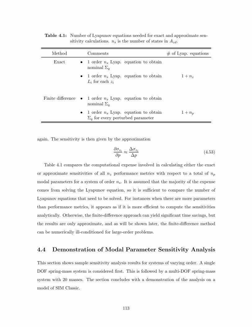
Table 4.1: Number of Lyapunov equations needed for exact and approximate sen-sitivity calculations. ns is the number of states in Azd.

Method Comments # of Lyap. equations

Exact • 1 order ns Lyap. equation to obtainnominal Σq

• 1 order ns Lyap. equation to obtainLi for each zi

1 + nz

Finite difference • 1 order ns Lyap. equation to obtainnominal Σq

• 1 order ns Lyap. equation to obtainΣq for every perturbed parameter

1 + np

again. The sensitivity is then given by the approximation

∂σzi

∂p≈ ∆σzi

∆p(4.53)

Table 4.1 compares the computational expense involved in calculating either the exact

or approximate sensitivities of all nz performance metrics with respect to a total of np

modal parameters for a system of order ns. It is assumed that the majority of the expense

comes from solving the Lyapunov equation, so it is sufficient to compare the number of

Lyapunov equations that need to be solved. For instances when there are more parameters

than performance metrics, it appears as if it is more efficient to compute the sensitivities

analytically. Otherwise, the finite-difference approach can yield significant time savings, but

the results are only approximate, and as will be shown later, the finite-difference method

can be numerically ill-conditioned for large-order problems.

4.4 Demonstration of Modal Parameter Sensitivity Analysis

This section shows sample sensitivity analysis results for systems of varying order. A single

DOF spring-mass system is considered first. This is followed by a multi-DOF spring-mass

system with 20 masses. The section concludes with a demonstration of the analysis on a

model of SIM Classic.

113

m w

zζ=1%

k

10−1

100

101

10−6

10−5

10−4

10−3

Frequency (Hz)

N2 /H

z

10−1

100

101

0

0.01

0.02

0.03Disturbance PSD’s and cumulative RMS curves

N

(a) (b)

Figure 4.2: (a) Single DOF system. (b) Disturbance PSD (bottom) and cumula-tive RMS (top).

4.4.1 Single DOF system

The simple mass-spring system of Figure 4.2(a) is identical to the one presented in Sec-

tion 3.2. The mass and stiffness values were chosen to obtain a natural frequency of 1 Hz,

and the modal damping is 1%. Recall that the performance is the position of the mass, and

the disturbance force w acts on the mass. This force is the output of a first-order system

driven by unit-intensity white noise. The PSD of the disturbance is shown in Figure 4.2(b).

Plotted above the disturbance PSD is the cumulative RMS curve.

Placing the disturbance filter in series with the plant leads to a form equivalent to

Eq. 4.6. Solving the Lyapunov equation given by Eq. 4.7 yields the state covariance matrix

Σq, which can then be substituted into Eq. 4.8 to determine the performance covariance

matrix Σz. Since there is only one performance metric in this case, Σz is a scalar and equals

the variance σ2z . For the specific numerical values in this problem, the RMS turns out to

be about 3.6 mm. The normalized sensitivities of this value with respect to the natural

frequency, damping ratio, and modal mass can be determined by solving for the Lagrange

multiplier matrix from Eq. 4.21 and then applying Eqs. 4.47–4.52.

The results are presented in bar chart form in Figure 4.3. The horizontal axis represents

the normalized sensitivity, and the vertical axis represents the open-loop mode with which

the modal parameters are associated. The mode is identified by its undamped natural

frequency. The values of the black, gray, and white bars are the normalized sensitivities

114

−2 −1.5 −1 −0.5 0

1

Ope

n−lo

op m

odal

freq

uenc

y (H

z)

pnom

/σz,nom

*∂ σz /∂ p

p = ωp = ζ p = m

Figure 4.3: Normalized sensitivities of SDOF system performance with respect tomodal parameters.

with respect to the natural frequency, damping ratio, and modal mass, respectively. All

three sensitivities are negative, which indicates that an increase in any parameter will cause

the RMS to decrease. However, the RMS sensitivity to the frequency is about four times

larger than the damping sensitivity and about twice as large as the modal mass sensitivity.

The bar chart indicates that raising the frequency by 1% will lower the RMS by 2%. Of

course in reality, the frequency cannot be changed directly. Rather, only physical properties

of the system (e.g., stiffness, mass) can be modified to affect the frequency. Another item of

practicality is that even though the sensitivities have been normalized to address the issue

of units, they still might not be comparable. For instance, does a 1% change in frequency

“equal” a 1% change in damping? If the sensitivities are to be used to identify parameters

for redesign, then an additional normalization step should be done that takes into account

engineering judgment to “equalize” parameter changes based on the apparent “cost” of

varying the parameters. For example, a 10% change in damping might be deemed to require

the same amount of resources as a 2% change in the frequency. If the sensitivities are to be

used to identify parameters for an uncertainty analysis, then the additional normalization

step might incorporate the uncertainty range for each parameter.

115

10−5

100

10−8

10−6

10−4

10−2

100

102

f = 1

Hz,

ζ =

1%

% Perturbation

Freq. Sens. % Errors

10−5

100

10−8

10−6

10−4

10−2

100

102

% Perturbation

Damping Sens. % Errors

Position of mass

Figure 4.4: Magnitudes of the percent errors in the finite-difference approxima-tion to the sensitivities with respect to frequency (left) and damping(right) as a function of parameter perturbation size.

Validation of the analytical sensitivities shown in Figure 4.3 involved computing a finite-

difference approximation (Eq. 4.53) by perturbing each parameter and determining the

resulting change in the RMS value. The magnitude of the percent error between the finite-

difference value and the exact value is shown as a function of perturbation size in Figure 4.4.

The errors in the sensitivities with respect to frequency and damping decrease as the per-

turbation size becomes smaller. This is expected because the ∆σzi∆p approximation to the

derivative should approach the exact answer in the limit as ∆p approaches 0. In reality,

numerical precision limitations can arise, and this might explain the “kink” in the curves

at a perturbation size of about 10−5%.

4.4.2 Multi-DOF system

To demonstrate the method on a slightly more complicated system, the 20 mass/19 spring

example problem in Figure 4.5(a) was created. Each mass and spring constant was randomly

selected from a specified interval. Modal damping was uniformly assigned a value of 0.1%.

There are six disturbance input locations at DOF’s 7 through 12. The performance metric

is the differential motion of the two end masses (i.e., z = x20 − x1). The PSD’s of the

six disturbances are shown in Figure 4.5(b). They are bandpass in nature, with the peak

magnitude occurring at 100 Hz and the low and high frequency asymptotes having values

of +4 and −4, respectively. Only two curves are visible because the first three disturbance

PSD’s overlap to form the larger magnitude curve, and the last three overlap to form the

116

smaller magnitude curve. The disturbance filter that created the PSD’s in Figure 4.5(b) was

augmented to the spring/mass system’s state-space representation. The frequency-domain

disturbance analysis discussed in Section 3.1.2 was used to create the plot in Figure 4.5(c),

which shows the PSD of the performance metric and its corresponding cumulative RMS

curve. The modal parameters associated with the first three modes were selected for the

sensitivity analysis because the largest contributions to the RMS are due to these modes.

The normalized sensitivities are presented in Figure 4.5(d), and the largest one corresponds

to the frequency of the third mode. All the normalized sensitivities are negative, and the

first mode is unique in that the sensitivity with respect to modal mass is larger in magnitude

than the sensitivity with respect to frequency.

Figure 4.6 shows the comparison between the exact sensitivities and the approximate

finite-difference sensitivities. Each row of subplots is associated with a particular mode

while each column is associated with either the frequency or damping parameter of the

mode. (Modal mass sensitivity errors are not shown, but they exhibit a similar trend.)

As the perturbation size becomes smaller, the trend is initially the same as that found for

the single DOF case. However, a point is reached when the errors start to climb as ∆p

decreases. Thus, numerical issues arise sooner for this larger order system. Nevertheless,

errors on the order of only 0.1% can be achieved by choosing a ∆pp of 0.1% for the finite-

difference approximation.

4.4.3 SIM Classic

The model used to demonstrate the sensitivity analysis methodology on a realistically-sized

problem is the three-baseline integrated model of SIM developed at JPL and described in

Chapter 2. Recall that some model parameters are:

• 10 Hz 6-axis isolator (50% damping) at the reaction wheel assembly location (IM-

PORTANT NOTE: The SIM model used in this chapter contains a slightly improved

isolator model. This results in a small shift in the frequencies of the open-loop modes.

The critical frequencies identified in the frequency-domain disturbance analysis of Sec-

tion 3.3 do not correspond exactly to the critical frequencies identified in this section.)

• 0.1% modal damping for structural modes

• 100 Hz bandwidth on fringe tracking control

117

x1

1m

ζ=0.1%

kkkk1

2x

m2

2

m

x

m

x

19

18

19

19

20

20

(a)

101

102

103

10−6

10−5

10−4

10−3

10−2

Frequency (Hz)

Mag

nitu

de (

N2 /Hz)

0

0.5

1

1.5Disturbance PSD’s and cumulative RMS curves

N

0

5

10

nm

Performance PSD and cumulative RMS curve

101

102

103

10−15

10−10

10−5

100

105

Frequency (Hz)

Mag

nitu

de (

nm2 /H

z)

(b) (c)

−1 −0.9 −0.8 −0.7 −0.6 −0.5 −0.4 −0.3 −0.2 −0.1 0

47.81

83.55

110.8

Normalized sensitivities

Ope

n−lo

op m

odal

freq

uenc

y (H

z)

pnom

/σz,nom

*∂ σz /∂ p

p = ωp = ζ p = m

(d)

Figure 4.5: (a) 20 DOF spring/mass system. (b) Disturbance PSD’s (bottom)and cumulative RMS (top). (c) Performance PSD (bottom) and cu-mulative RMS (top). (d) Normalized sensitivities of critical modes.

118

10−5

100

10−4

10−2

100

102

f = 4

7.8

Hz,

ζ =

0.1

%

Freq. Sens. % Errors

10−5

100

10−4

10−2

100

102

Damping Sens. % Errors

10−5

100

10−4

10−2

100

102

f = 8

3.5

Hz,

ζ =

0.1

%

10−5

100

10−4

10−2

100

102

10−5

100

10−4

10−2

100

102

f = 1

11 H

z, ζ

= 0

.1%

% Perturbation 10

−510

010

−4

10−2

100

102

% Perturbation

Total OPD (int. 1)

Figure 4.6: Magnitudes of the percent errors in the finite-difference approxima-tion to the sensitivities with respect to frequency (left) and damping(right) as a function of parameter perturbation size.

119

The optical path difference (OPD) of guide interferometer #1 is the performance metric

selected for the modal parameter sensitivity analysis.

In order to maintain the explicit modal parameter dependence in Azd, as indicated

in Eq. 4.41, the model could not be reduced using a technique such as balanced model

reduction [65]. However, since the Lyapunov equation can only be solved for strictly stable

systems, the translational rigid-body mode states had to be removed. It was assumed that

these modes are unobservable in the optical performance metrics of interest and can be

eliminated by a strict truncation. Since SIM constantly undergoes rigid-body translation

as it moves through inertial space, this should only cause SIM’s siderostats to sample a

different portion of the incoming stellar wavefront during an observation. This translation

should not affect differential pathlength or wavefront tilt metrics.

The strict truncation of rigid-body mode states led to Azd being of order 307 (= dis-

turbance states + modal states + compensator states). Solving a 307th order Lyapunov

equation took on average 110 seconds on a Sun Ultra 1. This is not an unreasonably long

computation time, but the restriction on model reduction can pose a problem for higher-

order systems. The sensitivity analysis technique that has been described relies on the

specific form of Azd. Application to much larger systems will require the technique to be

modified so that alternative model reduction approaches can be accommodated.

The reaction wheel assembly (RWA) disturbances are modeled by fourth-order band-

pass filters that approximate the analytical PSD’s derived in Section 2.2.5. Figure 4.7 plots

both the analytical PSD’s and the PSD’s of the filter. The six disturbances are the three

forces and three moments acting at the interface between the RWA and the spacecraft. Note

that the PSD’s are similar to those used in the multi-DOF case of the previous section.

The sensitivity analysis requires that the disturbances be modeled by shaping filters

driven by white noise. The analytical PSD’s have a characteristic “sawtooth” shape and

can not be represented exactly in state-space form. The “smooth” curves represent a simple,

low-order approximation to the more complex PSD’s. They are based on a disturbance filter

of the form

Gd(s) =As2

(s + ωo)4(4.54)

Gd(ω) =A(jω)2

(jω + ωo)4(4.55)

120

The approximate disturbance PSD’s are therefore of the form

Sww(ω) = Gd(ω)GHd (ω)

=

[A(jω)2

(jω + ωo)4

] [A(−jω)2

(−jω + ωo)4

]

=A2ω4

(jω + ωo)4(−jω + ωo)4(4.56)

The double zero at s = 0 creates the +4 slope in the PSD at low frequencies, while the

fourth-order pole causes the high frequency slope to be −4. The actual analytical PSD’s

drop to zero magnitude at the frequency corresponding to the highest harmonic of the

maximum wheel speed. A faster roll-off can be achieved in the approximate PSD’s by

using more poles; however, this comes at the cost of more states in the system. The corner

frequency ωo was arbitrarily chosen to be at the geometric mean of the frequencies of the

first and last “drops” in the analytical PSD’s. Referring to Figure 4.7, these frequencies

are at about 18 Hz and 720 Hz. This placed the center frequency of the band-pass filter in

a location that one might choose by visual inspection. The magnitudes of the filter-based

PSD’s were chosen such that the overall RMS values matched those of the analytical PSD’s.

In other words, both the analytical and the approximate PSD’s contain the same amount

of energy.

It can be seen that the “smooth” filter-based PSD’s do not fit the “sawtooth” analytical

PSD’s extremely well; however, a better result can be achieved with a higher-order shaping

filter model. Since the main goal of this section is to demonstrate the sensitivity analysis

technique, no further effort was made to obtain a close fit. In practice, further iterations

should be made in creating a more accurate disturbance filter model.

Rather than computing sensitivities with respect to parameters of all the modes in the

system, a frequency-domain disturbance analysis can be used first to identify which modes

are the most critical. The disturbance PSD’s are simply those corresponding to the approx-

imate PSD’s. They are shown alone in Figure 4.8(a), and the resulting PSD of the OPD

is presented in Figure 4.8(b). Also plotted in Figure 4.8(b) is the disturbance contribu-

tion plot that indicates which disturbances are dominant across the frequency range. It is

based on the approximation that the disturbance cross-spectral density matrix is diagonal.

The critical modes from the cumulative variance plot in Figure 4.9(a) are summarized in

Figure 4.9(b).

121

10−5

100

RM

S (

N o

r N

−m

)

100

101

102

103

10−12

10−10

10−8

10−6

10−4

10−2

Freq. (Hz)

Mag

nitu

de (

N2 /Hz

or (

N−

m)2 /H

z)

Figure 4.7: Analytical RWA disturbance PSD’s and approximate PSD’s from low-order filter (bottom). Cumulative RMS curves (top).

100

101

102

103

0

0.5

1

1.5Disturbance PSD’s and cumulative RMS curves

Forces in N

Moments in N−m

100

101

102

103

10−10

10−8

10−6

10−4

10−2

Frequency (Hz)

Mag

nitu

de RWA FxRWA FyRWA FzRWA MxRWA MyRWA Mz

0

5

nm

PSD and cumulative RMS (Total OPD (int. 1))

10−10

10−5

100

nm2 /H

z

100

101

102

FxFyFz

MxMyMz

Disturbance Contribution

Frequency (Hz)

Dis

turb

ance

(a) (b)

Figure 4.8: (a) Approximate PSD’s from low-order filter (bottom), and cumula-tive RMS curves (top). (b) Performance PSD (middle), cumulativeRMS (top), and disturbance contribution (bottom).

122

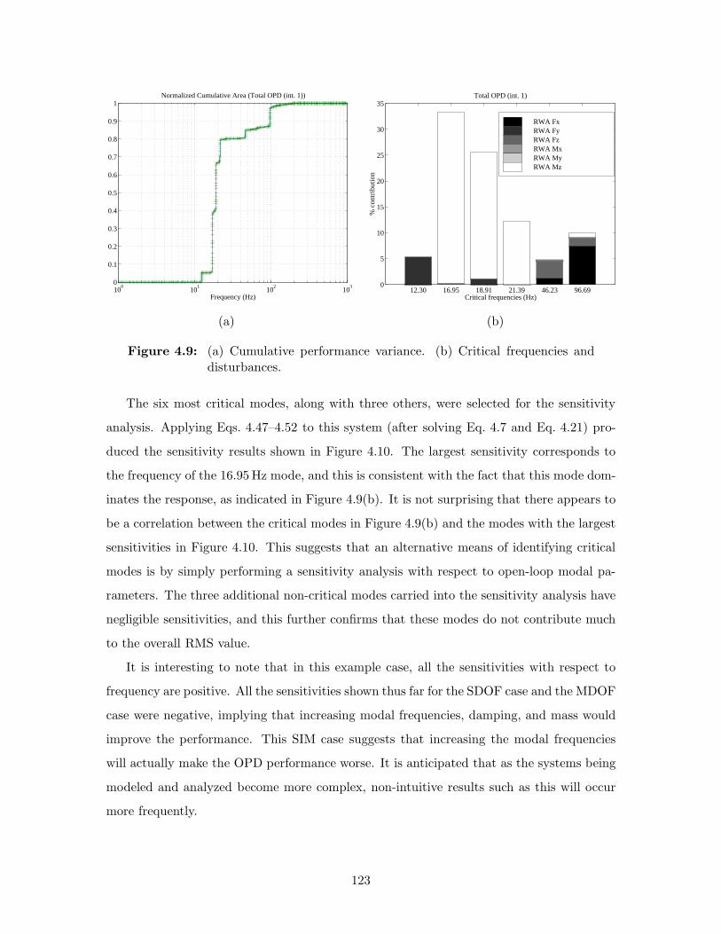
100

101

102

103

0

0.1

0.2

0.3

0.4

0.5

0.6

0.7

0.8

0.9

1

Frequency (Hz)

Normalized Cumulative Area (Total OPD (int. 1))

12.30 16.95 18.91 21.39 46.23 96.690

5

10

15

20

25

30

35

Critical frequencies (Hz)

% c

ontr

ibut

ion

Total OPD (int. 1)

RWA Fx RWA Fy RWA Fz RWA Mx RWA My RWA Mz

(a) (b)

Figure 4.9: (a) Cumulative performance variance. (b) Critical frequencies anddisturbances.

The six most critical modes, along with three others, were selected for the sensitivity

analysis. Applying Eqs. 4.47–4.52 to this system (after solving Eq. 4.7 and Eq. 4.21) pro-

duced the sensitivity results shown in Figure 4.10. The largest sensitivity corresponds to

the frequency of the 16.95 Hz mode, and this is consistent with the fact that this mode dom-

inates the response, as indicated in Figure 4.9(b). It is not surprising that there appears to

be a correlation between the critical modes in Figure 4.9(b) and the modes with the largest

sensitivities in Figure 4.10. This suggests that an alternative means of identifying critical

modes is by simply performing a sensitivity analysis with respect to open-loop modal pa-

rameters. The three additional non-critical modes carried into the sensitivity analysis have

negligible sensitivities, and this further confirms that these modes do not contribute much

to the overall RMS value.

It is interesting to note that in this example case, all the sensitivities with respect to

frequency are positive. All the sensitivities shown thus far for the SDOF case and the MDOF

case were negative, implying that increasing modal frequencies, damping, and mass would

improve the performance. This SIM case suggests that increasing the modal frequencies

will actually make the OPD performance worse. It is anticipated that as the systems being

modeled and analyzed become more complex, non-intuitive results such as this will occur

more frequently.

123

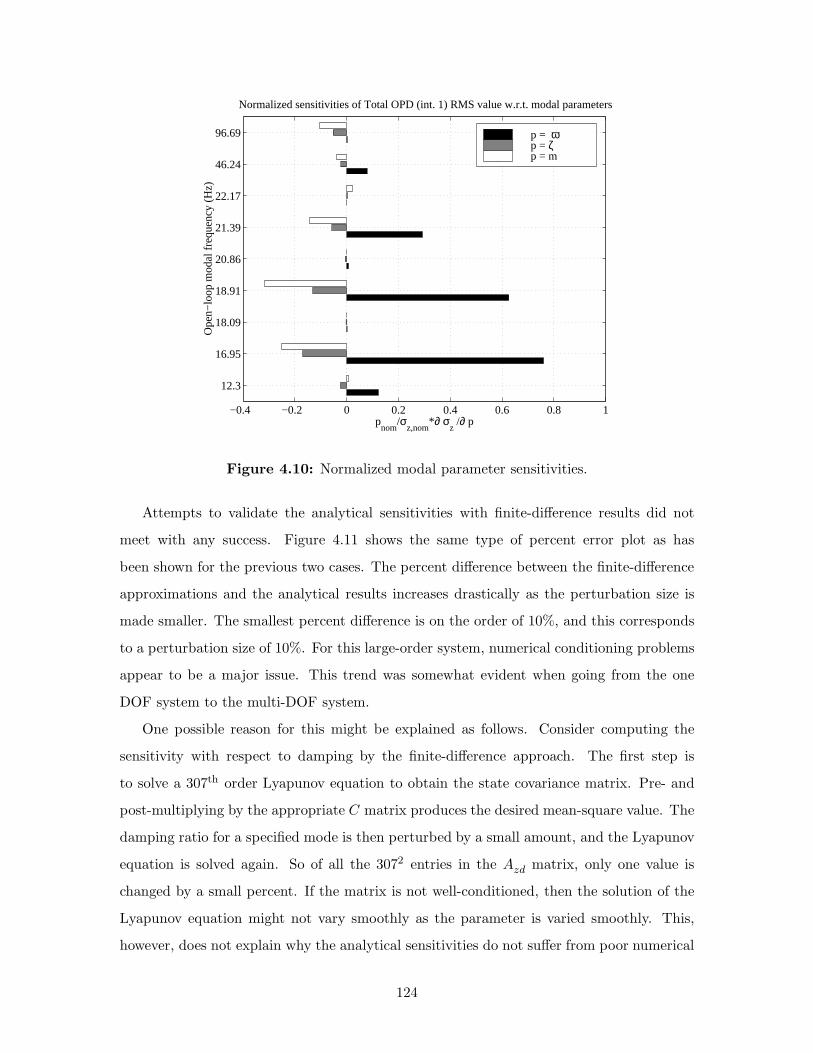
−0.4 −0.2 0 0.2 0.4 0.6 0.8 1

12.3

16.95

18.09

18.91

20.86

21.39

22.17

46.24

96.69

Normalized sensitivities of Total OPD (int. 1) RMS value w.r.t. modal parameters

Ope

n−lo

op m

odal

freq

uenc

y (H

z)

pnom

/σz,nom

*∂ σz /∂ p

p = ωp = ζ p = m

Figure 4.10: Normalized modal parameter sensitivities.

Attempts to validate the analytical sensitivities with finite-difference results did not

meet with any success. Figure 4.11 shows the same type of percent error plot as has

been shown for the previous two cases. The percent difference between the finite-difference

approximations and the analytical results increases drastically as the perturbation size is

made smaller. The smallest percent difference is on the order of 10%, and this corresponds

to a perturbation size of 10%. For this large-order system, numerical conditioning problems

appear to be a major issue. This trend was somewhat evident when going from the one

DOF system to the multi-DOF system.

One possible reason for this might be explained as follows. Consider computing the

sensitivity with respect to damping by the finite-difference approach. The first step is

to solve a 307th order Lyapunov equation to obtain the state covariance matrix. Pre- and

post-multiplying by the appropriate C matrix produces the desired mean-square value. The

damping ratio for a specified mode is then perturbed by a small amount, and the Lyapunov

equation is solved again. So of all the 3072 entries in the Azd matrix, only one value is

changed by a small percent. If the matrix is not well-conditioned, then the solution of the

Lyapunov equation might not vary smoothly as the parameter is varied smoothly. This,

however, does not explain why the analytical sensitivities do not suffer from poor numerical

124

10−5

100

100

105

f = 1

2.3

Hz,

ζ =

0.1

%Freq. Sens. % Errors

10−5

100

100

105

Damping Sens. % Errors

10−5

100

100

105

f = 1

7 H

z, ζ

= 0

.1%

10−5

100

100

105

10−5

100

100

105

f = 1

8.9

Hz,

ζ =

0.1

%

% Perturbation 10

−510

0

100

105

% Perturbation

Total OPD (int. 1)DWFT, x (int. 1) DWFT, y (int. 1) DBS, x (int. 1) DBS, y (int. 1)

Figure 4.11: Magnitudes of the percent errors in the finite-difference approxima-tion to the sensitivities with respect to frequency (left) and damping(right) as a function of perturbation size.

conditioning if it is present. Further investigation into this effect is recommended.

At this point, the results shown in Figure 4.10 cannot be verified, but since the sen-

sitivities are the expected order of magnitude, then some confidence can be placed in the

accuracy of the results. As will be shown in Section 5.4.4, the use of these analytical sensi-

tivities in an example SIM uncertainty analysis yields results that are consistent with those

obtained using another method. This will serve to indirectly validate the sensitivities.

4.5 Physical Parameter Sensitivities

Of particular use in the early design phases of a system is the ability to identify modifications

that can improve the performance of the system. This is especially true when it is discovered

125

during performance assessment analyses that the nominal design fails to meet specified

requirements. Identifying areas for redesign can be made easier if sensitivity information

is available. Sensitivities reveal the amount of change in the performance metrics that

can be achieved by varying parameters in a model of the system. Parameters with large

sensitivities can then be the focus of structural redesigns and/or uncertainty management.

Section 4.3 introduced a method to compute the exact sensitivities with respect to

open-loop modal parameters. While these sensitivities do identify which modes are the

most important, they do not reveal directly what physical characteristics of the design

should be modified to affect the modes and improve the performance. Physical parameter

sensitivities are therefore more intuitive, and this fact motivated the efforts to expand the

sensitivity analysis to include physical parameters.

The following section presents the mathematics behind computing sensitivities with

respect to physical parameters. The model is assumed to be in state-space form, and the

general case assumes that disturbance filter and compensator dynamics are also present. As

is shown, the derivatives of the finite-element model mode shapes, natural frequencies, and

modal masses with respect to the parameters are required. Section 4.5.2 reviews the theory

behind eigenvalue and eigenvector derivatives of structural systems with no repeated eigen-

values. The analytical sensitivities are then compared to finite-difference approximations

on a simple cantilever beam example. To explore issues faced when dealing with large-order

models, an integrated model of SIM Classic is used to demonstrate the technique. Potential

simplifications to the sensitivity equations are investigated in order to reduce computational

effort.

4.5.1 Derivation of physical parameter sensitivities

In Section 4.1, the overall state-space system was placed into the form

q = Azd q +Bzd d

z = Czd q (4.57)

126

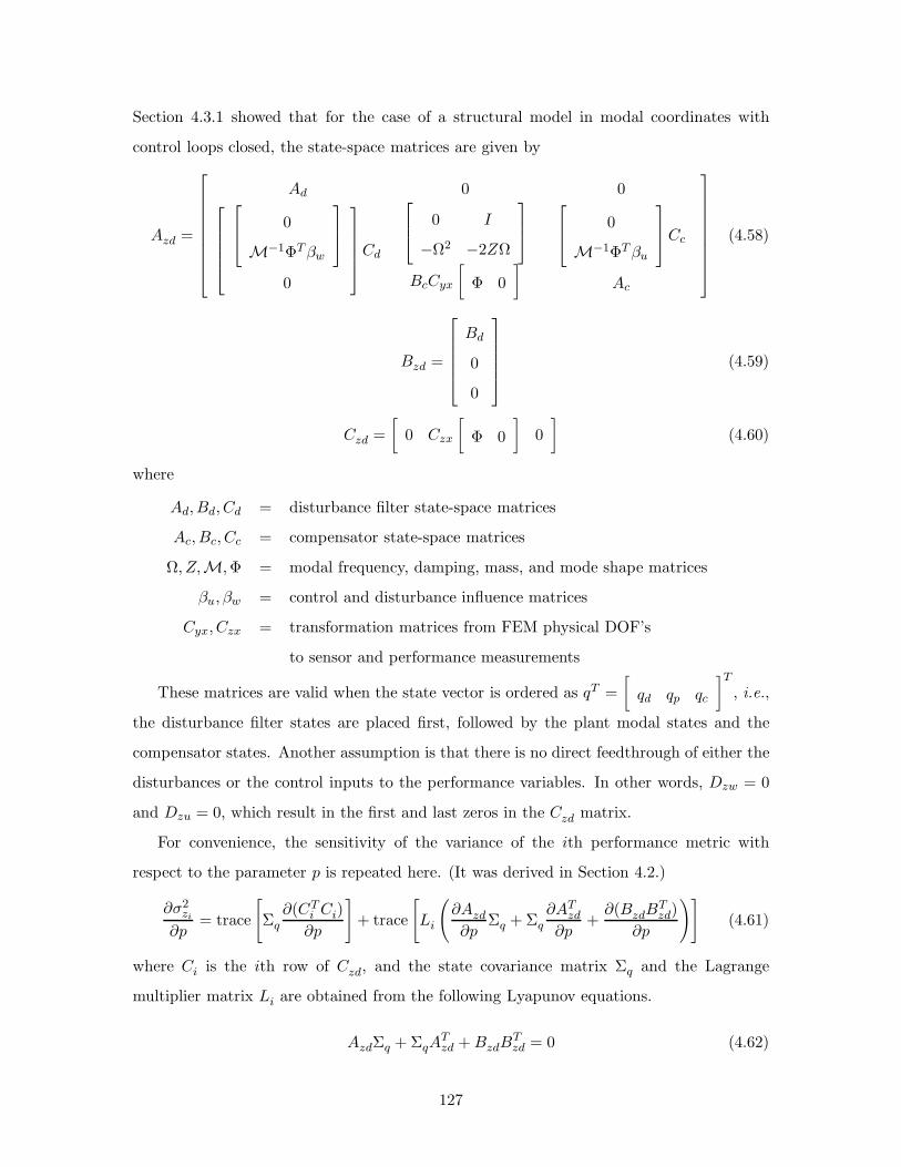
Section 4.3.1 showed that for the case of a structural model in modal coordinates with

control loops closed, the state-space matrices are given by

Azd =

Ad 0 0

0

M−1ΦTβw

0

Cd

0 I

−Ω2 −2ZΩ

BcCyx

[Φ 0

] 0

M−1ΦTβu

Cc

Ac

(4.58)

Bzd =

Bd

0

0

(4.59)

Czd =[

0 Czx

[Φ 0

]0]

(4.60)

where

Ad, Bd, Cd = disturbance filter state-space matrices

Ac, Bc, Cc = compensator state-space matrices

Ω, Z,M,Φ = modal frequency, damping, mass, and mode shape matrices

βu, βw = control and disturbance influence matrices

Cyx, Czx = transformation matrices from FEM physical DOF’s

to sensor and performance measurements

These matrices are valid when the state vector is ordered as qT =[qd qp qc

]T, i.e.,

the disturbance filter states are placed first, followed by the plant modal states and the

compensator states. Another assumption is that there is no direct feedthrough of either the

disturbances or the control inputs to the performance variables. In other words, Dzw = 0

and Dzu = 0, which result in the first and last zeros in the Czd matrix.

For convenience, the sensitivity of the variance of the ith performance metric with

respect to the parameter p is repeated here. (It was derived in Section 4.2.)

∂σ2zi

∂p= trace

[Σq

∂(CTi Ci)∂p

]+ trace

[Li

(∂Azd

∂pΣq + Σq

∂ATzd

∂p+∂(BzdB

Tzd)

∂p

)](4.61)

where Ci is the ith row of Czd, and the state covariance matrix Σq and the Lagrange

multiplier matrix Li are obtained from the following Lyapunov equations.

AzdΣq + ΣqATzd +BzdB

Tzd = 0 (4.62)

127

ATzdLi + LiAzd + CT

i Ci = 0 (4.63)

If p is a physical parameter of the finite-element model, then in general it will not appear

explicitly in the state-space matrices Azd, Bzd, or Czd. However, the mode shapes in Φ, the

modal frequencies in Ω , and the modal masses inM can depend on p. Thus, the parameter

dependence can be expressed in functional notation as

Azd → Azd(Φ(p),Ω(p),M(p)) (4.64)

Czd → Czd(Φ(p)) (4.65)

Notice that the modal damping matrix Z has not been mentioned yet. In most situa-

tions, damping is specified in terms of modal damping rather than as a physical damping

matrix C. As a result, Z will not be a function of a physical parameter in the model.

The damping ratios ζi are specified rather than derived. This is the reason why damping

parameter dependence will not be carried into the subsequent derivation.

Since Bzd is only a function of the disturbance filter Bd matrix, Eq. 4.61 can be simplified

to

∂σ2zi

∂p= trace

[∂Ci

∂pΣqC

Ti + CiΣq

∂CTi

∂p

]+ trace

[Li

(∂Azd

∂pΣq + Σq

∂ATzd

∂p

)](4.66)

The matrix derivatives ∂Ci∂p , ∂Azd

∂p , and their transposes need to be computed. By invoking

the chain rule based on the parameter dependence expressed in Eq. 4.64 and Eq. 4.65, the

derivatives can be written as

∂Azd

∂p=

N∑j=1

∂Azd

∂ωj︸ ︷︷ ︸†

∂ωj

∂p︸︷︷︸‡

+∂Azd

∂mj︸ ︷︷ ︸†

∂mj

∂p︸ ︷︷ ︸‡

+n∑

i=1

∂Azd

∂Φij︸ ︷︷ ︸†

∂Φij

∂p︸ ︷︷ ︸‡

(4.67)

∂Czd

∂p=

N∑j=1

n∑i=1

[0 ∂Cz

∂Φij0]

︸ ︷︷ ︸†

∂Φij

∂p︸ ︷︷ ︸‡

(4.68)

where N is the number of modes in Φ, and n is the number of degrees of freedom. Recall

that the matrices Ω and M in Eq. 4.58 are diagonal.

Ω =

. . .

ωj

. . .

, M =

. . .

mj

. . .

where j = 1, 2, . . . , N (4.69)

128

At this point, it is apparent that two types of derivatives are required. The first type

involves state-space matrix derivatives with respect to frequencies, mode shapes, and modal

masses (e.g., ∂Azd∂ωj

, ∂Azd∂mj

, ∂Azd∂Φij

, and ∂Czd∂Φij

). They are indicated by a † in Eqs. 4.67 and 4.68.

The second type involves the mode shape, frequency, and modal mass derivatives, namely∂Φij

∂p , ∂ωj

∂p and ∂m∂p . These are indicated by a ‡ in Eqs. 4.67 and 4.68. The first type will be

examined next, and Section 4.5.2 will discuss the mode shape, frequency, and modal mass

derivatives.

First examine the computation of ∂Azd∂ωj

and ∂Azd∂mj

. If Azd is of the form shown in Eq. 4.58,

then these derivatives are very straightforward to compute. In fact, they were required in

Section 4.3.2 for the sensitivities with respect to modal parameters, and the results shown

in Eq. 4.49 and Eq. 4.51 are repeated here.

∂Azd

∂ωj=

0 0 0

0

0

0

0 0

0

−2ωj

0

0

−2ζj

0

0

0

0

0

(4.70)

∂Azd

∂mj=

0 0 0

0

−φTj βw

0

Cd

0 0

0 0

0

0

−φTj βu

Cc

0

(4.71)

It is important to note that when using numerical software such as MATLAB, sparse matri-

ces can be used to alleviate the storage requirements of a matrix comprised almost entirely

of zeros. This also helps to reduce the time required to perform matrix manipulations.

The derivatives with respect to Φij can also be obtained by inspection. If we make the

standard assumption that the mode shapes are mass normalized such thatM = I, then

∂Azd

∂Φij=

0 0 0

0

(1n×Ni,j )Tβw

0

Cd

0 0

0 0

BcCyx

[(1n×N

i,j ) 0]

0

(1n×Ni,j )Tβu

Cc

0

(4.72)

129

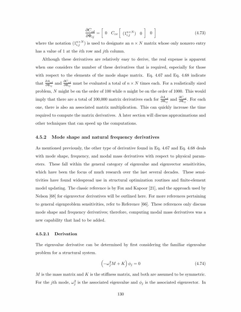
∂Czd

∂Φij=[

0 Czx

[(1n×N

i,j ) 0]

0]

(4.73)

where the notation (1n×Ni,j ) is used to designate an n×N matrix whose only nonzero entry

has a value of 1 at the ith row and jth column.

Although these derivatives are relatively easy to derive, the real expense is apparent

when one considers the number of these derivatives that is required, especially for those

with respect to the elements of the mode shape matrix. Eq. 4.67 and Eq. 4.68 indicate

that ∂Azd∂Φij

and ∂Czd∂Φij

must be evaluated a total of n×N times each. For a realistically sized

problem, N might be on the order of 100 while n might be on the order of 1000. This would

imply that there are a total of 100,000 matrix derivatives each for ∂Azd∂Φij

and ∂Czd∂Φij

. For each

one, there is also an associated matrix multiplication. This can quickly increase the time

required to compute the matrix derivatives. A later section will discuss approximations and

other techniques that can speed up the computations.

4.5.2 Mode shape and natural frequency derivatives

As mentioned previously, the other type of derivative found in Eq. 4.67 and Eq. 4.68 deals

with mode shape, frequency, and modal mass derivatives with respect to physical param-

eters. These fall within the general category of eigenvalue and eigenvector sensitivities,

which have been the focus of much research over the last several decades. These sensi-

tivities have found widespread use in structural optimization routines and finite-element

model updating. The classic reference is by Fox and Kapoor [21], and the approach used by

Nelson [68] for eigenvector derivatives will be outlined here. For more references pertaining

to general eigenproblem sensitivities, refer to Reference [66]. These references only discuss

mode shape and frequency derivatives; therefore, computing modal mass derivatives was a

new capability that had to be added.

4.5.2.1 Derivation

The eigenvalue derivative can be determined by first considering the familiar eigenvalue

problem for a structural system. (−ω2

jM +K)φj = 0 (4.74)

M is the mass matrix and K is the stiffness matrix, and both are assumed to be symmetric.

For the jth mode, ω2j is the associated eigenvalue and φj is the associated eigenvector. In

130

more familiar structural dynamic terminology, ωj is the natural frequency and is a diagonal

entry in the modal frequency matrix Ω. The vector φj is the mode shape and is a column

of the modal matrix Φ.

Differentiating both sides of Eq. 4.74 with respect to a structural parameter p and

pre-multiplying by φTj leads to

φTj

(−ω2

jM +K)

︸ ︷︷ ︸=[(−ω2

j M+K)φj]T =0

∂φj

∂p+ φT

j

(−ω2

j

∂M

∂p+∂K

∂p

)φj −

∂ω2j

∂pφT

j Mφj︸ ︷︷ ︸=1

= 0 (4.75)

and it can be seen that the unity modal mass normalization of the mode shapes has been

enforced. Solving for the eigenvalue derivative∂ω2

j

∂p produces the simple result

∂ω2j

∂p= φT

j

(−ω2

j

∂M

∂p+∂K

∂p

)φj (4.76)

Eq. 4.76 indicates that the derivative of the squared natural frequency of the jth mode is

given in terms of the corresponding mode shape and frequency as well as the mass and

stiffness derivatives with respect to the parameter p. It does not depend on knowing the

values of other modal frequencies and mode shapes.

Unfortunately, computing the mode shape derivative requires substantially more effort.

Prior to the pre-multiplication step that produced Eq. 4.75, the following intermediate

equation can be obtained.

(−ω2

jM +K)

︸ ︷︷ ︸≡Kj

∂φj

∂p=∂ω2

j

∂pMφj −

(−ω2

j

∂M

∂p+∂K

∂p

)φj︸ ︷︷ ︸

≡bj

(4.77)

Once Eq. 4.76 is evaluated, the right-hand side of Eq. 4.77 is known. Also, the coefficient

matrix in front of ∂φj

∂p is known. Eq. 4.77 is therefore of the form

Kj∂φj

∂p= bj (4.78)

where we will refer to Kj as the dynamic stiffness matrix associated with the jth mode.

Eq. 4.78 is a system of linear equations in terms of the elements of the vector ∂φj

∂p . A

direct solution can not be obtained via a procedure such as Gauss-Jordan elimination and

back substitution because Kj is a singular matrix. This is evident because Eq. 4.74 has

nonzero solutions for φj . In particular, Kj will have a rank of n− 1 if all the ωj are unique,

i.e., if there are no repeated eigenvalues [35]. If a particular problem does have repeated

131

eigenvalues, then alternative solution techniques are required. However, the remainder of

this section will only consider the case of distinct modal frequencies.

The solution procedure begins by assuming that ∂φj

∂p can be expressed as the sum of a

particular solution of Eq. 4.77 and a homogeneous solution. Since the mode shape vector φj

is in the nullspace of Kj , as indicated by Eq. 4.74, the homogeneous solution is φj multiplied

by an undetermined scalar a. Denote the particular solution as ψj and write ∂φj

∂p as

∂φj

∂p= ψj + aφj (4.79)

Differentiating the mass normalization relation φTj Mφj = 1 with respect to p produces

∂φTj

∂pMφj + φT

j

∂M

∂pφj + φT

j M∂φj

∂p= 0 (4.80)

Noting that the first term is just the transpose of the third term leads to

2φTj M

∂φj

∂p+ φT

j

∂M

∂pφj = 0 (4.81)

Replacing ∂φj

∂p by the right-hand side of Eq. 4.79 results in

2φTj M (ψj + aφj) + φT

j

∂M

∂pφj = 0 (4.82)

which can be expanded to give

2φTj Mψj︸ ︷︷ ︸

=0

+2aφTj Mφj︸ ︷︷ ︸

=1

+φTj

∂M

∂pφj = 0 (4.83)

To see why the first term is set to zero, notice that Eq. 4.79 explicitly separates the homo-

geneous solution aφj from the particular solution ψj . Hence, ψj does not have a component

in the direction of φj . In fact, ψj can be thought of as a linear combination of all of the

remaining eigenvectors since the mode shapes are linearly independent. In other words, ψj

is in the column space of the matrix[φ1 φ2 · · · φj−1 φj+1 · · · φm

](4.84)

All of these modes are mass orthogonal to φj ; therefore, φTj Mψj = 0. Solving Eq. 4.83 for

a produces

a = −12φT

j

∂M

∂pφj (4.85)

The technique used by Nelson in Reference [68] to obtain the particular solution ψj

involves constraining one of the elements of ψj to be zero. The element is arbitrarily chosen

132

to be the degree of freedom associated with the largest component (in magnitude) of the

mode shape φj. Imposing a value of zero allows a row and column of Kj to be removed,

thereby truncating Eq. 4.78 into a non-singular set of linear equations of the form

Kjψj = bj (4.86)

which can be solved using standard techniques such as Gauss-Jordan elimination (rather

than by inverting Kj). The vector ψj is then simply ψj with a zero inserted at the appro-

priate location.

Once the mode shape derivatives have been determined, the modal mass derivatives

readily follow. The modal mass equation is given by

mj = φTj Mφj (4.87)

Differentiating with respect to p leads to

∂mj

∂p= 2φT

j M∂φj

∂p+ φT

j

∂M

∂pφj (4.88)

Since ∂φj

∂p and ∂M∂p have already been calculated, the right-hand side is known.

To summarize, the eigenvalue derivative for each mode is computed using Eq. 4.76. The

mode shape derivative is computed by first solving for the scaling factor a in Eq. 4.85 to

obtain the homogeneous solution aφj. The particular solution ψj is obtained by solving

Eq. 4.86, which is the same as Eq. 4.77, but with one degree of freedom removed. The

modal mass derivative is given by Eq. 4.88.

4.5.2.2 Example Beam Element Derivatives

The key to being able to compute eigen-sensitivities with respect to physical parameters is

whether it is possible to evaluate the matrix derivatives ∂K∂p and ∂M

∂p . Notice that the term(−ω2

j∂M∂p + ∂K

∂p

)φj appears in both the equation for the eigenvalue derivative (Eq. 4.76)

and the right-hand side of the eigenvector derivative equation (Eq. 4.77). K and M are the

system stiffness and mass matrices in global coordinates and typically have contributions

from many different elements. What is usually done in practice is to first compute derivative

matrices at the element level, then transform to global coordinates, and keep a running sum

from all the contributing elements [48].

133

Table 4.2: DOF ordering for a single, two-node Bernoulli-Euler beam element.

# DOF Description

1 x1 Node 1 displacement in x

2 y1 Node 1 displacement in y

3 z1 Node 1 displacement in z

4 θx1 Node 1 rotation about x

5 θy1 Node 1 rotation about y

6 θz1 Node 1 rotation about z

7 x2 Node 2 displacement in x

8 y2 Node 2 displacement in y

9 z2 Node 2 displacement in z

10 θx2 Node 2 rotation about x

11 θy2 Node 2 rotation about y

12 θz2 Node 2 rotation about z

Take for example the element stiffness matrix for a two-node, constant cross-section,

Bernoulli-Euler beam element with shear deformation and rotary inertia effects ignored.

Assume that the local degrees of freedom are ordered as shown in Table 4.2.

The general form of the matrix is (see for example Reference [13])

Kelement =

EAL

−EAL

12EIzL3

6EIzL2 − 12EIz

L36EIzL2

12EIy

L3 − 6EIy

L2 − 12EIy

L3 − 6EIy

L2

GJL

−GJL

− 6EIy

L24EIy

L

6EIy

L22EIy

L

6EIz

L24EIz

L− 6EIz

L22EIz

L

−EAL

EAL

− 12EIzL3 − 6EIz

L212EIz

L3 − 6EIzL2

− 12EIy

L36EIy

L212EIy

L36EIy

L2

−GJL

GJL

− 6EIy

L22EIy

L

6EIy

L24EIy

L

6EIzL2

2EIzL

− 6EIzL2

2EIzL

(4.89)

134

The element mass matrix can either be created using a lumped mass approach or a

consistent mass formulation. The form of the element mass matrix used in IMOS (and

based on NASTRAN’s formulation) is

Melement =ρAL

420×

175 35

156 22L 54 −13L

156 −22L 54 13L

105(Iy+Iz)

A

−22L 4L2 −13L −3L2

22L 4L2 13L −3L2

35 175

54 13L 156 −22L

54 −13L 156 22L

105(Iy+Iz)

A

13L −3L2 22L 4L2

−13L −3L2 −22L 4L2

(4.90)

The entries that are boxed are the result of a NASTRAN technique that averages the

lumped mass and consistent mass entries associated with the axial (i.e., extensional) degrees

of freedom.

The parameter dependence of Kelement and Melement can be expressed as

Kelement → Kelement(A, J, Iy, Iz , E,G,L) (4.91)

Melement →Melement(ρ,A, Iy , Iz, L) (4.92)

where

A = cross-sectional area

J = cross-sectional torsional constant

Iy = cross-sectional bending moment of inertia about the y axis

Iz = cross-sectional bending moment of inertia about the z axis

E = Young’s modulus

G = shear modulus

L = element length

ρ = mass density

135

For simplicity, the element length L will be treated as constant; hence, no sensitivities

will be computed with respect to this parameter. The difficulty arises due to the fact that

a change in an element’s length affects the nodal locations of all elements “downstream”

of the element. This implies that the transformation from local to global coordinates for

each element is no longer a constant based on the original geometry of the model. The

transformation matrix becomes a function of the changes in element lengths, which greatly

increases the difficulty of the problem. This is one of the reasons why structural redesigns

based on changing the topology of a model are hard to implement using a gradient approach.

Nevertheless, the remaining beam element parameters can be accommodated in the

derivative equations previously introduced. Therefore, the physical parameter p satisfies

p ∈[A J Iy Iz E G ρ

]

The matrix derivatives ∂Kelement∂p and ∂Melement

∂p can be computed symbolically and stored in

an element library for subsequent use.

Having evaluated these derivatives, the next step is to transform to global coordinates

via the element transformation matrix Tk, which satisfies

φj,k = Tkφj,k (4.93)

where φj,k represents the entries of the jth mode shape that correspond to the kth beam

element’s DOF’s in local coordinates. The vector φj,k is simply the same vector expressed

in global coordinates. It can be shown that

(−ω2

j

∂M

∂p+∂K

∂p

)φj =

# of elements∑k=1

Tk

(−ω2

j

∂Melement

∂p+∂Kelement

∂p

)φj,k (4.94)

The left hand side of the equation is the term that appears in both the eigenvalue and eigen-

vector derivatives, as mentioned previously. The summation extends over all the elements

of interest containing the parameter p. Eq. 4.76 becomes

∂ω2j

∂p=

# of elements∑k=1

φTj,k

(−ω2

j

∂Melement

∂p+∂Kelement

∂p

)φj,k (4.95)

while Eq. 4.77 becomes

(−ω2

jM +K)

︸ ︷︷ ︸≡Kj

∂φj

∂p=∂ω2

j

∂pMφj −

# of elements∑k=1

Tk

(−ω2

j

∂Melement

∂p+∂Kelement

∂p

)φj,k (4.96)

136

4.5.2.3 Example Generalized Spring and Inertia Derivatives

Although element derivative matrices have been shown only for the case of beam elements,

the same procedure can be applied to more complicated elements such as plates. In addi-

tion, early generation finite-element models typically incorporate generalized spring (e.g.,

CELAS) and inertia (e.g., CONM) elements. In the most general form, each of these ele-

ments can be characterized by a 6 × 6 matrix. (The following equations are also valid for

matrices of other sizes.) Let them be denoted by KCELAS and MCONM, respectively. In-

troduce scalar factors α and β that are used to capture overall stiffness and mass increases

as represented by αKCELAS and βMCONM, where α and β are nominally equal to 1. If

p = α or β, then Eq. 4.95 and Eq. 4.96 can be written as

∂ω2j

∂α= φT

j,CELAS

∂(αKCELAS)∂α︸ ︷︷ ︸

=KCELAS

φj,CELAS (4.97)

∂ω2j

∂β= −ω2

jφTj,CONM

∂(βMCONM)∂β︸ ︷︷ ︸

=MCONM

φj,CONM (4.98)

Kj∂φj

∂α=

∂ω2j

∂αMφj − ∂(αKCELAS)

∂α︸ ︷︷ ︸=KCELAS

φj,CELAS (4.99)

Kj∂φj

∂β=

∂ω2j

∂βMφj + ω2

j

∂(βMCONM)∂β︸ ︷︷ ︸

=MCONM

φj,CONM (4.100)

The previous equations assume that KCELAS and MCONM are expressed in the global coor-

dinate frame. φj,CELAS represents the entries in φj that correspond to the CELAS DOF’s,

while φj,CONM represents the entries in φj that correspond to the CONM DOF’s.

4.5.3 Implementation

An IMOS-compatible series of MATLAB functions that compute structural eigenvalue and

eigenvector derivatives for beam elements was written by S. Kenny (MIT) and are doc-

umented in Reference [48]. The main piece of code is called nelson.m, and it was used

to obtain the results presented in the following sections. Furthermore, the code was also

modified to compute modal mass sensitivities (Eq. 4.88), and a new function nelson mod.m

was created to calculate sensitivities with respect to the α and β parameters associated

with CELAS and CONM elements.

137

Another modification that was made to nelson.m and implemented in nelson mod.m

involves accounting for rigid-body elements (RBE’s) that result in constraint equations

relating certain “master” DOF’s (called the nset) and “slave” DOF’s (called the mset).

RBE’s are often found in first-generation conceptual models since much of the detailed

design has yet to be done. Certain components of the model are simply treated as behaving

like a rigid body.

To see how the constraint relations affect the equations for eigenvalue and eigenvector

derivatives, first write the standard undamped, unforced equations of motion for a finite-

element model.

Mx+Kx = 0 (4.101)

Assume the mass and stiffness matrices are partitioned according to the nset and mset

DOF’s.

M =

Mnn Mnm

Mmn Mmm

K =

Knn Knm

Kmn Kmm

x =

xn

xm

(4.102)

A constraint matrix Tc relates the nset DOF’s to the mset DOF’s.

xm = Tc xn (4.103)

The physical DOF’s x can therefore be expressed in terms of xn.

x =

I

Tc

︸ ︷︷ ︸

≡R

xn (4.104)

Reducing out the mset DOF’s from Eq. 4.101 results in

RTMR︸ ︷︷ ︸M

xn +RTKR︸ ︷︷ ︸K

xn = 0 (4.105)

138

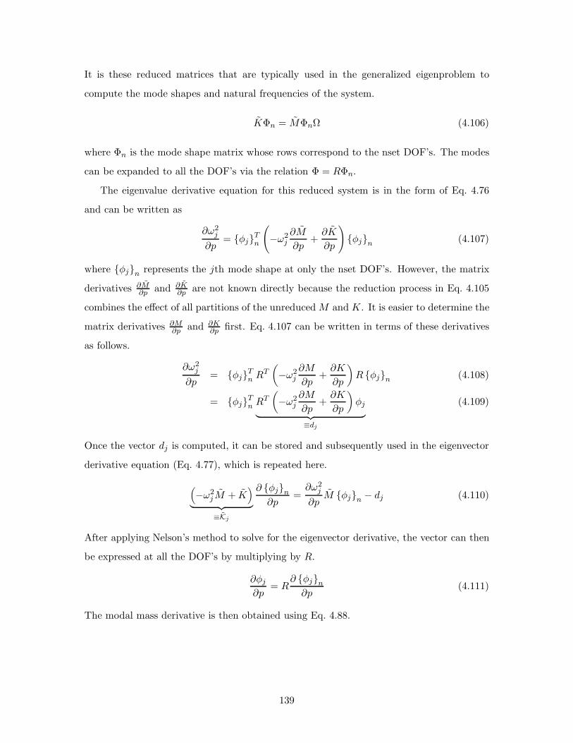
It is these reduced matrices that are typically used in the generalized eigenproblem to

compute the mode shapes and natural frequencies of the system.

KΦn = MΦnΩ (4.106)

where Φn is the mode shape matrix whose rows correspond to the nset DOF’s. The modes

can be expanded to all the DOF’s via the relation Φ = RΦn.

The eigenvalue derivative equation for this reduced system is in the form of Eq. 4.76

and can be written as

∂ω2j

∂p= φjTn

(−ω2

j

∂M

∂p+∂K

∂p

)φjn (4.107)

where φjn represents the jth mode shape at only the nset DOF’s. However, the matrix

derivatives ∂M∂p and ∂K

∂p are not known directly because the reduction process in Eq. 4.105

combines the effect of all partitions of the unreduced M and K. It is easier to determine the

matrix derivatives ∂M∂p and ∂K

∂p first. Eq. 4.107 can be written in terms of these derivatives

as follows.

∂ω2j

∂p= φjTn RT

(−ω2

j

∂M

∂p+∂K

∂p

)R φjn (4.108)

= φjTn RT(−ω2

j

∂M

∂p+∂K

∂p

)φj︸ ︷︷ ︸

≡dj

(4.109)

Once the vector dj is computed, it can be stored and subsequently used in the eigenvector

derivative equation (Eq. 4.77), which is repeated here.

(−ω2

j M + K)

︸ ︷︷ ︸≡Kj

∂ φjn∂p

=∂ω2

j

∂pM φjn − dj (4.110)

After applying Nelson’s method to solve for the eigenvector derivative, the vector can then

be expressed at all the DOF’s by multiplying by R.

∂φj

∂p= R

∂ φjn∂p

(4.111)

The modal mass derivative is then obtained using Eq. 4.88.

139

4.6 Demonstration of Physical Parameter Sensitivity Anal-

ysis

4.6.1 Cantilever beam

To validate the equations that have been presented for physical parameter sensitivities, a

cantilever beam example was created. The beam depicted in Figure 4.12(a) is assumed to

be made from aluminum, with density 2700 kg/m3, Young’s modulus 70 GPa, length 0.50 m,

width 1 cm, and height 1.8 cm. The primary bending direction is in the horizontal plane

(i.e., the plane perpendicular to the page). The disturbance is a tip force oriented at a

45 angle in the plane of the cross-section. It is bandlimited white noise with intensity

10−4 N2/Hz across the frequency range of the beam dynamics, as shown in Figure 4.12(b).

The performance metric is the tip displacement (in millimeters) along the same direction.

The RMS is 0.43 mm, as indicated in Figure 4.12(c). The beam is modeled with a single

Bernoulli-Euler beam element with six DOF’s at the tip node. The use of additional finite

elements would lead to better estimates of the modal frequencies; however, the purpose of

the model is to demonstrate the physical parameter sensitivities. Consequently, a single

beam element model was deemed sufficient. The stiffness and mass matrices are of the form

given in Eq. 4.89 and Eq. 4.90. Due to the fixed end, the first six rows and columns of

Kelement and Melement are deleted.

The modal frequencies and mode shape descriptions are listed in Table 4.3. Only the

first four modes are disturbable and observable, which is the reason why just four resonant

peaks are visible in the performance PSD plot.

Performing a sensitivity analysis of the tip displacement RMS with respect to modal

parameters results in the normalized sensitivities presented in Figure 4.13(a). As is evident,

the first mode is the most dominant, followed by the second mode. Perturbing the frequency,

modal mass, or damping of the higher modes has no appreciable affect. To confirm the mode

shape descriptions in Table 4.3, the strain energy contribution from the four primary types

of beam deformation (1 axial, 2 bendings, 1 twist) are displayed in Figure 4.13(b). Due

to the form of the element stiffness matrix given in Eq. 4.89, the modes are uncoupled,

meaning that there are no extension/twist or bending/twist coupled modes. The first four

modes are characterized by bending, the fifth mode is an axial mode, and the sixth mode

is a torsion mode.

140

h

y

x

LF (white noise)

δb

(a)

102

104

106

10−5

10−4

Frequency (Hz)

Mag

nitu

de (

N2 /Hz) 10

110

210

310

40

0.2

0.4

mm

101

102

103

104

10−15

10−10

10−5

100

Frequency (Hz)

Mag

nitu

de (

mm2 /H

z)

(b) (c)

Figure 4.12: (a) Cantilever beam demonstration case. (b) Tip force disturbancePSD. (c) Tip displacement cumulative RMS (top) and PSD (bot-tom).

141

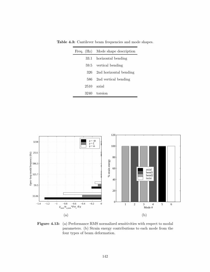
Table 4.3: Cantilever beam frequencies and mode shapes.

Freq. (Hz) Mode shape description

33.1 horizontal bending

59.5 vertical bending

326 2nd horizontal bending

586 2nd vertical bending

2510 axial

3240 torsion

−1.4 −1.2 −1 −0.8 −0.6 −0.4 −0.2 0

33.06

59.5

325.7

586.3

2511

3238

Ope

n−lo

op m

odal

freq

uenc

y (H

z)

pnom

/σz,nom

*∂ σz /∂ p

p = ωp = ζ p = m

1 2 3 4 5 60

20

40

60

80

100

120

Mode #

% s

trai

n en

ergy

axialbend1bend2twist

(a) (b)

Figure 4.13: (a) Performance RMS normalized sensitivities with respect to modalparameters. (b) Strain energy contributions to each mode from thefour types of beam deformation.

142

Table 4.4: Notation used for the four types of beam deformation. (jth mode, kthbeam element)

element DOF’s mode shape components element stiffness submatrix

axial (1,7) φj,k,axial Kk,axial

bending 1 (2,6,8,12) φj,k,bend1 Kk,bend1

bending 2 (3,5,9,11) φj,k,bend2 Kk,bend2

twist (4,10) φj,k,twist Kk,twist

The strain energy contributions are determined as follows. First consider the mode

shape partitioning shown symbolically below.

φj1−→ φj,k

2−→ φj,k3−→ φj,k,axial, φj,k,bend1, φj,k,bend2, φj,k,twist

Specifically, for the jth mode shape φj , the steps are:

1. Extract a vector of size 12 × 1 that corresponds to the 12 DOF’s of the kth beam

element.

2. Transform the vector to local element coordinates.

3. Split this vector into four separate vectors, each of which corresponds to the DOF’s

of one of the deformation types.

In addition, the rows and columns associated with the different sets of DOF’s can be ex-

tracted from the element stiffness matrix (recall Eq. 4.89) to form smaller stiffness subma-

trices. The notation is summarized in Table 4.4. The modal strain energies for the different

types of motion are simply

Uj,k,axial =12φT

j,k,axialKk,axialφj,k,axial (4.112)

Uj,k,bend1 =12φT

j,k,bend1Kk,bend1φj,k,bend1 (4.113)

Uj,k,bend2 =12φT

j,k,bend2Kk,bend2φj,k,bend2 (4.114)

Uj,k,twist =12φT

j,k,twistKk,twistφj,k,twist (4.115)

Dividing through by the total modal strain energy

Uj,total =12φT

j Kφj =12ω2

j (4.116)

143

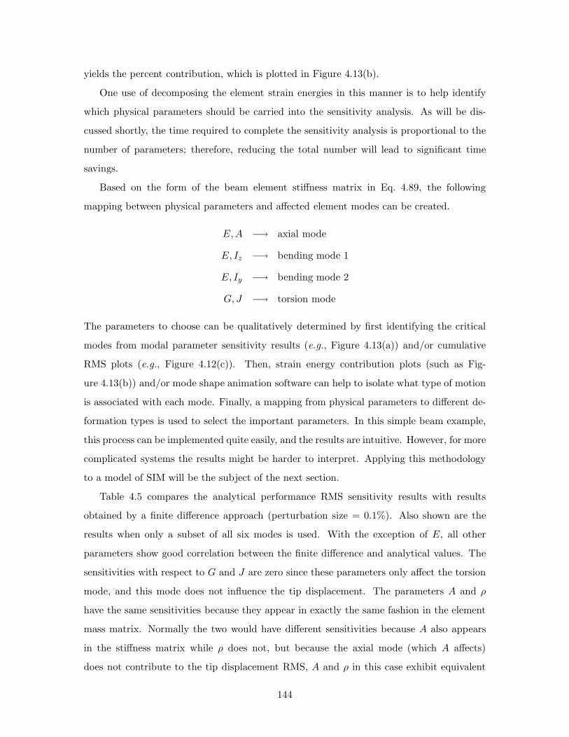
yields the percent contribution, which is plotted in Figure 4.13(b).

One use of decomposing the element strain energies in this manner is to help identify

which physical parameters should be carried into the sensitivity analysis. As will be dis-

cussed shortly, the time required to complete the sensitivity analysis is proportional to the

number of parameters; therefore, reducing the total number will lead to significant time

savings.

Based on the form of the beam element stiffness matrix in Eq. 4.89, the following

mapping between physical parameters and affected element modes can be created.

E,A −→ axial mode

E, Iz −→ bending mode 1

E, Iy −→ bending mode 2

G,J −→ torsion mode

The parameters to choose can be qualitatively determined by first identifying the critical

modes from modal parameter sensitivity results (e.g., Figure 4.13(a)) and/or cumulative

RMS plots (e.g., Figure 4.12(c)). Then, strain energy contribution plots (such as Fig-

ure 4.13(b)) and/or mode shape animation software can help to isolate what type of motion

is associated with each mode. Finally, a mapping from physical parameters to different de-

formation types is used to select the important parameters. In this simple beam example,

this process can be implemented quite easily, and the results are intuitive. However, for more

complicated systems the results might be harder to interpret. Applying this methodology

to a model of SIM will be the subject of the next section.

Table 4.5 compares the analytical performance RMS sensitivity results with results

obtained by a finite difference approach (perturbation size = 0.1%). Also shown are the

results when only a subset of all six modes is used. With the exception of E, all other

parameters show good correlation between the finite difference and analytical values. The

sensitivities with respect to G and J are zero since these parameters only affect the torsion

mode, and this mode does not influence the tip displacement. The parameters A and ρ

have the same sensitivities because they appear in exactly the same fashion in the element

mass matrix. Normally the two would have different sensitivities because A also appears

in the stiffness matrix while ρ does not, but because the axial mode (which A affects)

does not contribute to the tip displacement RMS, A and ρ in this case exhibit equivalent

144

sensitivities. They have negative sensitivities, which agrees with the modal mass sensitivities

found in Figure 4.13(a). These sensitivities are negative, which implies that increasing the

modal mass will decrease the RMS. But an increased modal mass can be achieved by

increasing either ρ or A, and the physical parameter sensitivities in Table 4.5 also indicate

that increasing these quantities will reduce the RMS.

The largest sensitivities correspond to E and Iy, and this supports the findings in

Figure 4.13. Mode 1, which is the dominant mode, is characterized by bending mode

type 2. The physical parameter mapping indicates that E and Iy affect this mode, and

bending about the y-axis corresponds to the “weak” bending direction.

The columns in Table 4.5 that correspond to the analytical predictions are based on

retaining all or only a subset of the modes when evaluating the Azd and Czd matrix deriva-

tives in Eq. 4.67 and Eq. 4.68. These derivatives involve summing over 1 to N , where N

is the total number of modes. The column headings that take integer values from 1 to 6

indicate what value of N was used to compute the sensitivity values in the columns of the

table. For instance, the column with the heading “4” means that only the first four modes

were used in the calculations.

This is the first attempt at investigating time-saving simplifications that can be exploited

in models of appreciable size. As shown previously, the first two modes are the dominant

contributors to the tip displacement RMS. The analytical approximation that only uses

these two modes produces reasonably accurate sensitivities. The maximum error does not

exceed 0.4%. Even the approximation that only retains the first mode does a good job of

estimating most of the sensitivities. Notice that the sensitivity with respect to Iz goes to

zero in this one-mode approximation since Iz has no effect on the primary bending mode.

These results suggest that only the modes in the frequency range where most of the

RMS contribution occurs need to be used in Eq. 4.67 and Eq. 4.68 in order to obtain good

estimates of the sensitivities. While this appears to hold for this simple example, the next

section will explore how valid the assumption is for the more complicated SIM model.

Although not used here, a time-saving measure which does not introduce any approxi-

mations is based on looping only over the DOF’s in Eq. 4.67 and Eq. 4.68 at which

• disturbances enter (based on βw),

• control inputs are applied (based on βu),

145

Table 4.5: Comparison of tip displacement RMS normalized sensitivities with re-spect to beam properties.

pnom

σz,nom

∆σz∆p

pnom

σz,nom

∂σz∂p (analytical), # of modes =

p (finite diff.) 6 5 4 3 2 1

A −0.2498 −0.2500 −0.2500 −0.2500 −0.2499 −0.2490 −0.2127

J 1.08 × 10−7 0 0 0 0 0 0

Iz −0.1099 −0.1100 −0.1100 −0.1100 −0.1096 −0.1096 0

Iy −0.6394 −0.6400 −0.6400 −0.6400 −0.6400 −0.6375 −0.6375

E −0.7493 −0.6739 −0.6739 −0.6739 −0.6738 −0.6713 −0.6375

G 1.08 × 10−7 0 0 0 0 0 0

ρ −0.2498 −0.2500 −0.2500 −0.2500 −0.2499 −0.2490 −0.2127

−0.8 −0.6 −0.4 −0.2 0 0.2

A

J

Iz

Iy

E

G

rho

Tip displacement RMS sensitivities

pnom

/σz,nom

∂ σz / ∂ p

finite diff.6 modes 5 modes 4 modes 3 modes 2 modes 1 mode

Figure 4.14: Bar chart representation of Table 4.5.

146

• sensor measurements are made (based on Cyx),

• and performance metrics are obtained (based on Czx).

These DOF’s are the ones that are important in Azd and Czd. The DOF’s that fall into

these categories should only be a fraction of the total number of DOF’s. The remaining

DOF’s contribute nothing because ∂Azd∂Φij

= 0 and ∂Czd∂Φij

= 0 for values of i that correspond

to these DOF’s.

As a simple illustrative example, consider a system which is open loop (hence no βu or

Cyx) and which has a single disturbance and collocated performance metric. Assume there

are 1000 DOF’s, and the disturbance and performance are associated with DOF #100.

Then βw and Czx contain only one nonzero element at the 100th entry.

βTw = Czx = [0 · · · 0 1 0 · · · 0]

↑ 100th element(4.117)

The terms ΦTβw and CzxΦ which appear in Eqs. 4.58 and 4.60 are given by

CzxΦ =(ΦTβw

)T=[

Φ(100,1) · · · Φ(100,1000)

]= 100th row of Φ (4.118)

Thus, the second summation in Eq. 4.67 and Eq. 4.68 needs to be evaluated only when

i = 100. This leads to significant time savings with no loss of accuracy.

4.6.2 SIM Classic

Results of a physical parameter sensitivity analysis on the model of SIM Classic will now

be presented. Figure 4.15 summarizes the results of the disturbance analysis and modal

parameter sensitivity analysis that have previously been done. Figure 4.15(a) shows the

familiar finite-element model and ray trace. Approximate PSD’s of RWA disturbance forces

and moments are plotted in Figure 4.15(b), and the resulting PSD of the OPD is shown in

Figure 4.15(c). The modal parameter sensitivities are presented in Figure 4.15(d)

To help identify which stiffness-related physical parameters should be used in the sen-

sitivity analysis, the percent strain energy stored in various elements was computed. Fig-

ure 4.16(a) shows the distribution of strain energy for the 16.95 Hz mode. The left subplot

shows the contribution from all the beam elements in the model. Elements 1–14 correspond

to the beam elements on the −x siderostat boom, elements 15–28 correspond to those on

the +x siderostat boom, and elements 29–37 correspond to those on the metrology boom.

147

SIM Optical Model Ray Trace

100

101

102

103

0

0.5

1

1.5Disturbance PSD’s and cumulative RMS curves

Forces in N

Moments in N−m

100

101

102

103

10−10

10−8

10−6

10−4

10−2

Frequency (Hz)

Mag

nitu

de RWA FxRWA FyRWA FzRWA MxRWA MyRWA Mz

(a) (b)

0

5

nm

PSD and cumulative RMS (Total OPD (int. 1))

10−10

10−5

100

nm2 /H

z

100

101

102

FxFyFz

MxMyMz

Disturbance Contribution

Frequency (Hz)

Dis

turb

ance

−0.4 −0.2 0 0.2 0.4 0.6 0.8 1

12.3

16.95

18.09

18.91

20.86

21.39

22.17

46.24

96.69

Normalized sensitivities of Total OPD (int. 1) RMS value w.r.t. modal parameters

Ope

n−lo

op m

odal

freq

uenc

y (H

z)

pnom

/σz,nom

*∂ σz /∂ p

p = ωp = ζ p = m

(c) (d)

Figure 4.15: (a) Stellar ray trace through guide interferometer #1 of SIM. (b)Approximate PSD’s (bottom) and cumulative RMS (top) of reactionwheel disturbances. (c) Performance PSD (bottom) and cumulativeRMS (top). (d) Normalized sensitivities of performance RMS withrespect to modal parameters of critical modes.

148

0 20 400

1

2

3

4

5

6

Beam element #

% s

trai

n en

ergy

axialbend1bend2twist

1 2 3 4 5 6 70

1

2

3

4

5

6

Sid. celas element #

% s

trai

n en

ergy

1 2 3 4 5 60

1

2

3

4

5

6

Hex. celas element #

% s

trai

n en

ergy

dx dy dz drxdrydrz

Mode #19, Freq 16.946907 Hz, Scaling factor 10.36622x y

z

(a) (b)

Figure 4.16: (a) Strain energy contributions for the 16.95 Hz mode. (b) Modeshape of the 16.95 Hz mode.

All the beam elements are ordered beginning at the root of each boom. Eqns. 4.112–4.115

were used to calculate the strain energy in the four different types of beam deformation, and

the results indicate that all the siderostat boom elements are in torsion while the metrology

boom is in bending. Most of the siderostat boom elements contain more than twice the

strain energy stored in the metrology boom elements. This suggests that the parameters

which should have a large effect on this mode are G and J of the siderostat boom. Recall

that G and J will have the same sensitivities because only the product GJ appears in a

beam element’s stiffness matrix. Examining the mode shape in Figure 4.16(b) reveals that

the siderostat booms are indeed undergoing torsion, and the boom tips are 180 out of

phase.

The middle subplot in Figure 4.16(a) shows the strain energy fraction stored in each

of the siderostat bay generalized spring elements. The SIM model includes these CELAS

elements to try to capture local flexibility between a siderostat bay and the supporting

siderostat boom. Since these CELAS elements are in the form of a fully-populated 6 × 6

stiffness matrix, the strain energy could not be decomposed into contributions from de-

formations such as extension and twist. Instead, the total strain energy in each CELAS

element was computed as12φT

j,CELASKCELASφj,CELAS (4.119)

149

The largest strain energy fraction is found in siderostat CELAS element #3. In Fig-

ure 4.16(b), this siderostat is the third one from the left, and in Figure 4.15(a), it is the

leftmost one through which stellar light is passing. The siderostat bays are numbered start-

ing with the outboard bay on the +x arm, proceeding to the inboard bay on the +x arm,

then starting with the outboard siderostat on the −x arm and proceeding to the inboard

siderostat on the same arm. Other potential parameters for the sensitivity analysis are the

α and β parameters associated with this siderostat bay. As discussed previously, these are

scalar factors that multiply the nominal KCELAS and MCONM matrices to capture overall

stiffness and mass increases or decreases.

The next largest contributor to the strain energy is siderostat CELAS element #6,

and this is the other siderostat that forms the pair for the guide interferometer shown in

Figure 4.15(a). The relative motion of the siderostats is difficult to see in the displayed

mode shape in Figure 4.16(b), so it is harder to verify the strain energy results based on

this picture; however, the use of modal animation software to zoom into areas of the model

did confirm the results.

The right subplot of Figure 4.16(a) shows the contributions from another class of strain

energy storage elements, namely the hexapod strut elements. These are also modeled with

CELAS elements, but instead of being characterized by a full 6×6 stiffness matrix, the end

of each strut is joined to a coincident node with a diagonalKCELAS in local strut coordinates.

This permits the contributions to be further decomposed into differential motion in each of

the six axes. However as expected, the plot shows that the strain energy is dominated by

axial (i.e., dx) deformation of the six struts that form the hexapod. The modal animation

software (called XVIEW) does not use visible line elements to represent spring elements,

and this is the reason why the hexapod appears to be “discontinuous” in Figure 4.16(b).

The two other dominant modes at 18.91 Hz and 21.39 Hz are characterized by local

modes of the siderostat bays, as shown in Figure 4.17. Both the mode shapes and the

siderostat CELAS strain energy plots clearly indicate which bays have the largest motion.

Siderostats 1 and 3 participate the most at 18.91 Hz, while siderostats 5 and 6 participate

the most at 21.39 Hz. The motion of the siderostats is comprised mostly of rotation about

x with some displacement in y. Recall that siderostats 3 and 6 collect the light for guide

interferometer #1; consequently, any motion by them will have a strong effect on the OPD.

The results of the physical parameter sensitivity analysis are presented in Figure 4.18.

150

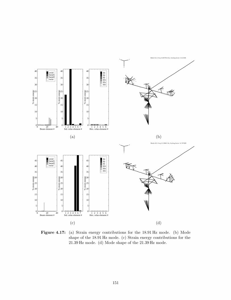
0 20 400

5

10

15

20

25

30

35

40

Beam element #

% s

trai

n en

ergy

axialbend1bend2twist

1 2 3 4 5 6 70

5

10

15

20

25

30

35

40

Sid. celas element #

% s

trai

n en

ergy

1 2 3 4 5 60

5

10

15

20

25

30

35

40

Hex. celas element #

% s

trai

n en

ergy

dx dy dz drxdrydrz

Mode #21, Freq 18.907816 Hz, Scaling factor 14.25589x y

z

(a) (b)

0 20 400

5

10

15

20

25

30

35

40

45

Beam element #

% s

trai

n en

ergy

axialbend1bend2twist

1 2 3 4 5 6 70

5

10

15

20

25

30

35

40

45

Sid. celas element #

% s

trai

n en

ergy

1 2 3 4 5 60

5

10

15

20

25

30

35

40

45

Hex. celas element #

% s

trai

n en

ergy

dx dy dz drxdrydrz

Mode #23, Freq 21.39061 Hz, Scaling factor 14.707899x y

z

(c) (d)

Figure 4.17: (a) Strain energy contributions for the 18.91 Hz mode. (b) Modeshape of the 18.91 Hz mode. (c) Strain energy contributions for the21.39 Hz mode. (d) Mode shape of the 21.39 Hz mode.

151

Two different sets of modes were used in the computations, and the plot shows that no

appreciable change in the predicted sensitivities occurs when more modes are used. This

confirms that the dominant modes are present in both sets of modes. Although the strain

energy contributions suggest that only certain parameters should be important, more are

included in the figure to check if the intuitive choices are correct. Parameters A through ρ

are the material and geometric properties of the siderostat boom. Parameters a1 through

a7 represent the α factors for each of the seven siderostat bay CELAS elements. Parameters

b1 through b7 represent the β factors for each of the seven siderostat bay CONM elements.

Note that hexapod stiffness parameters and metrology boom parameters were not included

in the analysis.

Figure 4.18 does confirm that G and J are the most important parameters of the sidero-

stat boom. Also, α3 and β3 have relatively large sensitivities. Since siderostat bay 3 has

large strain energy contribution in two out of the three critical modes, it makes sense that

the OPD is very sensitive to α3. The large sensitivity with respect to β3 is also intuitive and

can be explained as follows. In the local mode at 18.91 Hz, the siderostat bay undergoes

large motion relative to the siderostat boom to which it is attached. Changing the mass

and inertia properties (which β3 controls) of the bay should affect this motion. It is inter-

esting that the α3 and β3 sensitivities are opposite in sign, but this is not contradictory. A

positive sensitivity with respect to β3 suggests that decreasing the mass and inertia of the

bay will improve the performance. This should lead to an increase in the frequency of the

local siderostat mode. A negative sensitivity with respect to α3 suggests that increasing the

stiffness of the siderostat mount will also improve the performance, but this should increase

the frequency of the local mode as well. These results imply that the local dynamics of the

siderostat bays are important. What is surprising is that the sensitivities with respect α5

and β5 (the stiffness and mass parameters associated with siderostat 5) are fairly large. This

siderostat is not part of guide interferometer #1; however, it does undergo motion in the

two critical modes at 16.95 Hz and 21.39 Hz. The sensitivities suggest that the frequency of

this mount mode should be lowered, which is opposite of what should be done to siderostat

bay 3. The results might be indicating that the local mount modes should be individually

“tuned” to improve the performance.

The next largest parameter sensitivities for the siderostat boom correspond to the cross-

sectional area A and material density ρ of the siderostat boom beam elements. Since

152

−1.5 −1 −0.5 0 0.5 1 1.5

b7 b6 b5 b4 b3 b2 b1 a7 a6 a5 a4 a3 a2 a1rho G E Iy Iz J

A

Par

amet

er #

pnom

/σz,nom

*∂ σz/∂ p

Normalized Sensitivities of Total OPD (int. 1) RMS value w.r.t to physical parameters

modes 11−40 modes 11−50

Figure 4.18: SIM physical parameter sensitivities.

extension of the siderostat boom does not contribute to the critical mode at 16.95 Hz,

extensional strain energy is negligible; therefore, A was not identified as an important

parameter. A only affects the axial stiffness term EAL . What has been neglected thus far in

determining important parameters is a kinetic energy distribution analysis. From a kinetic

energy standpoint, the quantity ρA appears in every entry of a beam element’s mass matrix

(see Eq. 4.90) except for the torsion-related terms. Since the sensitivities with respect to ρ

and A are nearly identical, a possible explanation is that the total mass of the siderostat

booms is important. The siderostat booms not only deform in torsion in the 16.95 Hz mode,

but they also translate in the xy plane due to rotation of the structure about the z axis.

Positive sensitivities with respect to G and J and negative sensitivities with respect to ρ

and A appear to indicate that a performance improvement can be achieved with a decrease

in the frequency of the dominant mode. This agrees with the frequency sensitivity in

Figure 4.15(d), which indicates that increasing the frequency of the 16.95 Hz mode should

increase the performance RMS. On the other hand, the physical parameter sensitivities

for the third siderostat bay imply that the mount frequency should be increased. This

contradicts the fact that all the modal frequency sensitivities are positive. This contradiction

153

could point out a limitation in the modal parameter sensitivity analysis. The underlying

assumption is that a single parameter is being varied (either modal mass, frequency, or

damping) while everything else remains constant. This cannot happen in reality since the

mode shapes, frequencies, and modal masses are all interdependent. The physical parameter

sensitivity technique that has been developed takes this interdependence into account, and

therefore should be a more physically-based analysis. Further work should be conducted

in order to explore this issue further. It should be mentioned that similar results occurred

during experimental validation, and this issue will be discussed in Chapter 6 as well.

4.7 MATLAB Implementation

The modal parameter sensitivity analysis framework developed in this chapter has been

implemented in MATLAB within a function called sens analysis.m. The function can

compute the sensitivities analytically using the equations derived earlier in Section 4.3.

It assumes that the parameters are either modal damping ratios, natural frequencies, or

modal masses of open-loop structural modes. It also requires the state-space Azd matrix

to be of the form indicated in Eq. 4.41. The disturbance states should be placed first,

followed by the open-loop modal states and the compensator states (if the system is closed-

loop). The augmented disturbance/plant system should be stable, and this requires that

the system have no right-half plane or jω-axis poles. These states should be eliminated from

the system prior to calling the function. There is also an option to check the analytical

sensitivity results by performing finite-difference approximations. Some of the inputs to the

function are analogous to the inputs to the disturbance analysis function dist analysis.m.

The physical parameter sensitivity analysis framework has been implemented in a func-

tion called sens analysis phys.m. As before, the state-space system should be strictly

stable. This function requires the most detailed information about the state-space system

being considered. The disturbance analysis technique only requires a state-space represen-

tation and does not place any restrictions on the form of the individual state-space matrices.

The modal parameter sensitivity technique requires the plant model to be in a particular

modal form, but additional details regarding sensors, actuators, disturbances, and perfor-

mances are not needed. The function sens analysis phys.m, on the other hand, does

require knowledge of this type of information, particularly in the form of the matrices βu,

154

βw, Czx, and Cyx. It also must be given the mode shapes corresponding to the modal

frequencies in the plant Azw matrix.

Rather than computing the mode shape, frequency, and modal mass derivatives with

respect to physical parameters, sens analysis phys.m accepts these as inputs. It assumes

that they have been calculated previously using eigenvalue/eigenvector derivative functions

such as nelson.m [48] and nelson mod.m.

4.8 Summary

A method for calculating the exact sensitivities of performance RMS values with respect

to open-loop modal parameters has been presented. The approach was done in a state-

space framework, and the sensitivities were shown to require the solution of one Lyapunov

equation to obtain the state covariance matrix and one Lyapunov equation for every perfor-

mance metric. Derivatives of the state-space matrices with respect to a desired parameter

are simplified when the parameter is a modal parameter and the structural open-loop state-

space A matrix is in a standard modal form. Disturbances on the system are required to

be modeled as a linear filter driven by unit-intensity white noise. A MATLAB function

called sens analysis.m has been written to implement the methodology, and results were

shown when the code was used on a simple one DOF system, a multi-DOF system, and a

realistic SIM Classic model. Finite-difference approximations to the sensitivities helped to

validate the code for the first two systems; however, numerical conditioning problems with

the finite-difference methodology precluded the validation for the SIM Classic case.

A method has also been presented which determines the exact sensitivity values of

RMS outputs of a state-space model with respect to physical parameters of a structural

finite-element model. Since the state-space model assumes that the structural equations

of motion have been cast in modal form, the derivatives of the FEM mode shapes and

natural frequencies with respect to the parameters were required. Standard eigenvalue

and eigenvector derivative techniques were described, and an existing IMOS-compatible

MATLAB function was implemented to calculate these derivatives with respect to beam

element parameters. The capability to compute sensitivities with respect to scalar factors

that multiply generic CELAS and CONM element matrices was also added. The code was

also modified to account for rigid-body elements that relate certain DOF’s to other DOF’s.

155

A cantilever beam problem served to validate the analytical sensitivity equations. The

predictions agreed well with the approximate sensitivities from a finite-difference approach.

In addition, the use of only a subset of the total number of modes when calculating the

sensitivities still produced accurate results. This suggested that only important modes

need to be retained in the computations, and significant time savings are possible for large-

order models. The simple beam example was also used to demonstrate a process to select

the physical parameters for the sensitivity analysis. A disturbance analysis and a modal

parameter sensitivity analysis were first conducted to identify critical modes. Calculating

the strain energy distribution in these modes then helped to select the physical parameters

based on the type of deformation that the elements undergo in each mode.

Repeating this process on the more complicated SIM model revealed that a bandlimited

reaction wheel type disturbance caused several modes to be dominant in the OPD perfor-

mance metric that was chosen. This was confirmed in both a cumulative RMS plot of the

performance as well as the sensitivities with respect to modal parameters. Plots of the

strain energy contribution and the mode shape indicated that one mode was characterized

by siderostat boom torsion while two others were dominated by local siderostat bay motion.

Even though this suggested certain parameters for the sensitivity analysis, all parameters

were used in order to confirm the intuitive choices. A few additional sensitive parameters

were identified and suggested that kinetic energy distributions should be computed as well.

Furthermore, apparent contradictions between physical parameter and modal parameter

sensitivity results suggested that identifying redesign options for complex systems should

be based on the physical parameter sensitivity results. The modal parameter sensitivity

technique is more of an artificial rather than a physical analysis.

A next step is to “close the loop” on an overall system improvement algorithm. Thus

far, the modal parameter and physical parameter sensitivity analyses have been used to

provide a design engineer with a sense of which modes are most important and which struc-

tural parameters should be the focus of potential redesigns. What would be beneficial is an

algorithm that takes the results and then interfaces with the uncertainty analysis method-

ology in Chapter 5 to suggest the combination of design changes that satisfies performance

requirements subject to specified uncertainties and constraints. Chapter 7 takes a first step

toward achieving this goal.

156

Chapter 5

Uncertainty Analysis Framework

Disturbance analyses during early design stages of aerospace systems are typically con-

ducted on simplified models of nominal point designs. The models attempt to capture the

behavior of interest, and although they are generally suitable for judging relative merits

between competing designs in a trade study, the validity of their use in making absolute

performance predictions is not as clear. A way to account for uncertainties when assessing

performance would therefore be beneficial.

What is desired is a method to propagate uncertainties through a system model and

place bounds on the nominal performance predictions. A disturbance analysis is first con-

ducted to determine the nominal values, and an uncertainty analysis is then used to place

the equivalent of “error bars” around the nominal performance values. If it is found that

performance requirements are met even under worst-case model uncertainties, then confi-

dence in design margins can be increased.

A number of cases can be envisioned for the results of the disturbance and uncertainty

analyses, and they are depicted in Figure 5.1. The horizontal axis represents several different

designs, and the vertical axis represents a particular performance metric. In design 1, the

nominal performance does not meet the specified requirement. Also, the upper bound due

to the worst-case uncertainties falls above the requirement line. Since the design fails to

meet requirements, the system is redesigned, and design 2 is the result. In this case, the

nominal performance does satisfy the requirement; however, the upper bound does not. It

is this situation that highlights the need for an uncertainty analysis. Performing only the

nominal disturbance analysis would lead to the misconception that the design is satisfactory,

157

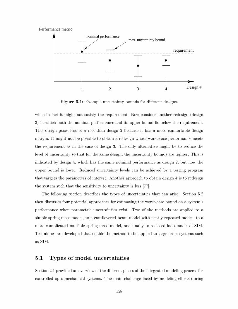
1 32 4 Design #

Performance metric

requirement

max. uncertainty boundnominal performance

Figure 5.1: Example uncertainty bounds for different designs.

when in fact it might not satisfy the requirement. Now consider another redesign (design

3) in which both the nominal performance and its upper bound lie below the requirement.

This design poses less of a risk than design 2 because it has a more comfortable design

margin. It might not be possible to obtain a redesign whose worst-case performance meets

the requirement as in the case of design 3. The only alternative might be to reduce the

level of uncertainty so that for the same design, the uncertainty bounds are tighter. This is

indicated by design 4, which has the same nominal performance as design 2, but now the

upper bound is lower. Reduced uncertainty levels can be achieved by a testing program

that targets the parameters of interest. Another approach to obtain design 4 is to redesign

the system such that the sensitivity to uncertainty is less [77].

The following section describes the types of uncertainties that can arise. Section 5.2

then discusses four potential approaches for estimating the worst-case bound on a system’s

performance when parametric uncertainties exist. Two of the methods are applied to a

simple spring-mass model, to a cantilevered beam model with nearly repeated modes, to a

more complicated multiple spring-mass model, and finally to a closed-loop model of SIM.

Techniques are developed that enable the method to be applied to large order systems such

as SIM.

5.1 Types of model uncertainties

Section 2.1 provided an overview of the different pieces of the integrated modeling process for

controlled opto-mechanical systems. The main challenge faced by modeling efforts during

158

conceptual design phases is the lack of detailed information about the design. When a

model is created of the design, there will undoubtedly be errors between the model and the

actual physical system if it was to be manufactured based on the nominal design. Since

the actual system is not available to provide data, the model cannot be updated to better

reflect the physical system.

In the most general sense, a model uncertainty represents an unknown error in a model of

a physical system. We broadly divide model uncertainty into parametric and non-parametric

uncertainties. A parametric uncertainty is an uncertainty in a parameter of the model. The

parameter can appear either explicitly in the state-space matrices or the matrices can be

implicit functions of the parameter. For example, if the system in Eq. 4.6 has an Azd matrix

of the form shown by Eq. 4.41, then an uncertainty in the frequency of a mode will manifest

itself as an uncertainty in two parameters of the Azd matrix. A physical parameter such as a

stiffness does not appear explicitly in the modal state-space matrices; however, uncertainty

in this parameter does have an affect on the mode shapes and frequencies, which do appear

in the matrices.

Non-parametric uncertainties cannot be captured by an uncertainty in one or more

parameters. For example, uncertainty in the model order implies that the number of states

might be incorrect (i.e., q is not the right length). This type of uncertainty can capture

modeling errors such as modal truncation, lack of fidelity, and incorrect finite-element types.

However, it is difficult to specify a form for this uncertainty. The error in representing a

nonlinear system with a linear model is another example of a non-parametric uncertainty.

The preliminary work presented in this thesis focuses on uncertainties in the open-loop

modal parameters of a structure. A goal is to enable the uncertainty analysis framework

to be compatible with the disturbance and sensitivity analysis methods described in the

previous chapters. The parameters are modal mass m, modal damping ζ, and natural

frequency ω. The next section discusses methods to find the worst case RMS performance

metrics σzi when m, ζ, and ω are not known exactly.

5.2 Parametric Uncertainty Analysis Methods

A few potential approaches have been identified that can determine the worst-case perfor-

mance due to parametric uncertainties. They include

159

2p

p p

p

"corner"

p

p

2,UB

2,LB1,LB 1,UB

1

Figure 5.2: Parameter space for the case of two uncertain parameters.

• Exhaustive search of all “corners” of the uncertain parameter space

• First-order Taylor series approximation

• Constrained optimization problem

• Robust control tools for bounds on H2 performance

5.2.1 Evaluation of “bad corners”

To understand the motivation behind this approach, consider the case of two uncertain

parameters each of which has a lower and an upper bound as indicated in Figure 5.2. The

actual values of the parameters can lie anywhere within the space of the box. What is

assumed is that the worst-case performance will occur when the parameters are at one of

the corners of this box. For example, this is the technique used by Bryson and Mills in

Reference [9] when designing robust LQG controllers via a minimax method. The LQG cost

was evaluated at all of the corners to determine the maximum cost due to the uncertainties.

This approach is very straightforward to implement; however, it can be inefficient for

large order systems with many uncertain parameters. If there are N parameters, then the

total number of corners at which the performance must be evaluated is 2N . Evaluating the

performance at each corner implies that a separate disturbance analysis has to be conducted

2N times. The computation time can be reduced; however, if appropriate model reduction

techniques are implemented, as discussed in a subsequent section.

Another issue is the fact that the worst-case is assumed to occur at one of these corners.

Reference [19] proves this for the simple case of SISO systems with no damping, but this

will not be true in general. A simple counter-example consisting of a cantilevered beam

160

with nearly repeated modes is presented in Section 5.4.2. The next approach, which utilizes

sensitivity information, can help to identify the potential “bad corner” a priori, thereby

eliminating the need to perform 2N disturbance analyses.

5.2.2 First-order approach

The first-order approach expresses the performance RMS values as a Taylor series approx-

imation about the nominal values.

σz = σz,nom +∂σz

∂p(p− pnom) + H.O.T. (5.1)

where σz is a vector containing the RMS values for each performance metric. The vector

p contains all of the uncertain parameters, and ∂σz∂p is referred to as the sensitivity matrix.

A technique for computing the sensitivities with respect to modal and physical parameters

was presented in Chapter 4. Neglecting the higher order terms and making the substitutions

∆σz = σz − σz,nom and ∆p = p− pnom results in

∆σz ≈ ∂σz

∂p∆p (5.2)

The parameter uncertainty is captured by ∆p, and in all approaches it is assumed that ∆p

is specified. For example, if all parameters are uncertain to within ±1% of the nominal

values, then for the ith parameter, ∆pi ∈ [−0.01 + 0.01]pi,nom. We seek to determine the

worst-case ∆σz for ∆p within the specified bounds. One way to define the worst-case ∆σz

is as the maximum magnitude of ∆σz over all allowable ∆p. However, a problem with this

definition is that a negative ∆σzi has the same effect as a positive ∆σzi . The magnitude

of a vector is only dependent on the squared values of the individual elements. We are

actually interested in not only the maximum magnitude, but also in having as many of

the individual elements as possible be positive. One option is to define the worst-case ∆σz

to be the vector that has the largest sum. To enable performance metrics with different

units to be summed, first define a normalization vector r. For instance, r could contain the

performance RMS requirements as follows

rT =

[1

σz1,req

· · · 1σznz,req

](5.3)

where nz is the number of performance metrics. Then a scalar “cost” J can be defined as

J = rT ∆σz =∆σz1

σz1,req

+ · · ·+ ∆σznz

σznz,req

(5.4)

161

Expanding Eq. 5.2,

∆σz1 = ∂σz1∂p1

∆p1 + ∂σz1∂p2

∆p2 + · · · + ∂σz1∂pnp

∆pnp

......

......

∆σznz = ∂σznz∂p1

∆p1 + ∂σznz∂p2

∆p2 + · · · + ∂σznz∂pnp

∆pnp

(5.5)

where np denotes the total number of uncertain parameters. Computing the cost J results

in the following expression.

J =

(1

σz1,req

∂σz1

∂p1+ · · ·+ 1

σznz,req

∂σznz

∂p1

)︸ ︷︷ ︸

≡a1

∆p1 + · · · (5.6)

+

(1

σz1,req

∂σz1

∂pnp+ · · ·+ 1

σznz,req

∂σznz

∂pnp

)︸ ︷︷ ︸

≡anp

∆pnp (5.7)

= a1∆p1 + · · ·+ anp∆pnp (5.8)

To maximize J , it is sufficient to maximize each of the ai∆pi terms. This assumes that the

∆pi’s occur independently; however, in reality, this might not be the case. For instance,

if some of the uncertain parameters are modal frequencies, then specifying independent

frequencies might not be physically realizable. This inconsistency will be allowed for the

present purpose of finding the worst-case performance.

The ∆p vector that maximizes J is therefore given by

∆pi =

∆pi,LB , if sgn(ai) = −1

∆pi,UB , if sgn(ai) = +1

undefined , if ai = 0

(5.9)

Substituting the worst-case ∆p into Eq. 5.2 produces an estimate of the increase in RMS

values due to the uncertainties. Thus, since the worst-case ∆p is simply some combination

of the bounds of the uncertain parameters, this approach identifies the “bad corner.”

To summarize, the first-order approach approximates the change in performance RMS

values as the product of a sensitivity matrix with a vector of parameter changes. The worst-

case performance is defined as the maximum weighted sum of performance RMS values for

parameter values within a specified uncertainty range. This leads to a simplistic linear

programming problem whose solution places the worst-case uncertainties at either their

lower or upper bounds. Instead of evaluating Eq. 5.8 at these bounds, a more accurate

162

value can be obtained simply by redoing a disturbance analysis with the system parameters

set to the values at the “bad corner.”

An advantage of this approach is that it is simple to implement once the sensitivities are

computed. Also, it provides a worst-case estimate for each of the performance metrics. As

will be shown, this is not possible for the robust control approach, which places a bound on

the sum of the performance variances. The main disadvantage is the accuracy that can be

obtained. Section 5.4 will compare the results obtained from this approach with the results

from the constrained optimization approach. As the uncertainty ranges become larger, the

first-order approach fails to accurately predict the worst-case performance.

5.2.3 Constrained optimization approach

This approach attempts to find a solution to the following optimization problem:

max J = trace(Σz)p

subject to pLB ≤ p ≤ pUB

(5.10)

where as before p is a vector of uncertain parameters, and pLB and pUB are the lower and

upper bounds, respectively, of the parameters. The covariance matrix Σz is based on the

transformation z = Rz, where R is a diagonal matrix used, for example, to normalize the

performance metrics so as to include weightings or to remove units. One choice for R could

be to place the elements of the r vector (described previously) along the diagonal of R.

Then Σz = RΣzRT = RCzdΣqC

TzdR

T . The system is assumed to be of the form described

by Eq. 4.6.

Eq. 5.10 expresses our desire to determine the set of allowable parameters that maximizes

the sum of normalized performance variances. A technique that can be used to solve Eq. 5.10

is based on the Sequential Quadratic Programming (SQP) method, and the MATLAB

function constr.m is an implementation of the method (see Reference [26]).

If the SQP method converges to a solution, it is not necessarily the global maximum.

Local maxima may exist, and the SQP routine may converge to these depending on the

initial guess that is provided to the routine. The only recourse is to begin with random

initial guesses that are within the feasible space and then to check the consistency of the

solutions that are obtained.

163

SQP is iterative in nature, and at each step the cost J and its gradient are computed.

The major computation expense arises from solving the Lyapunov equation (Eq. 4.7) for the

state covariance matrix. For large order systems, the solution time can be quite long. Also,

if the routine is not provided with gradient information, it must be computed numerically.

As will be shown, this reduces the efficiency of the routine. Whenever possible, gradients

(i.e., sensitivities) should be computed analytically; however, the sensitivity calculations

also require the solution of Lyapunov equations. The next section will suggest possible

model reduction strategies and approximations that can reduce the computational burden

for the case of systems with a large number of states.

As in the first-order case, a benefit of the constrained optimization method is that it pro-

vides an estimate of the worst-case parameters, p. In addition, the individual performance

RMS values for the worst-case p can be obtained by creating the system in Eq. 4.6 with

the new parameters p instead of the nominal values. Then the solution to the Lyapunov

equation, Eq. 4.7, is determined. The worst-case performance covariances follow directly

from Eq. 4.8.

5.2.4 Robust control approach

Reference [87] describes a method for computing a bound on theH2 performance of a system

with real parametric uncertainties. It builds upon the work in Reference [37]. A summary

of the theory is presented in this section.

Begin by considering the system described by Eq. 4.6, but with real parametric uncer-

tainties in the nominal Azd matrix. The new system is of the form

q = (Azd + ∆Azd) q +Bzd d

z = Czd q (5.11)

∆Azd is a real matrix which is assumed to be expressed in the form

∆Azd = B∆∆C∆ (5.12)

The ∆ matrix can be thought of as a feedback block around the nominal system, as shown

in Figure 5.3. Do not confuse the ∆ matrix with the notation used to describe the change

in a matrix (e.g., ∆Azd ≡ Azd,actual − Azd,nominal). It should be evident from the context

164

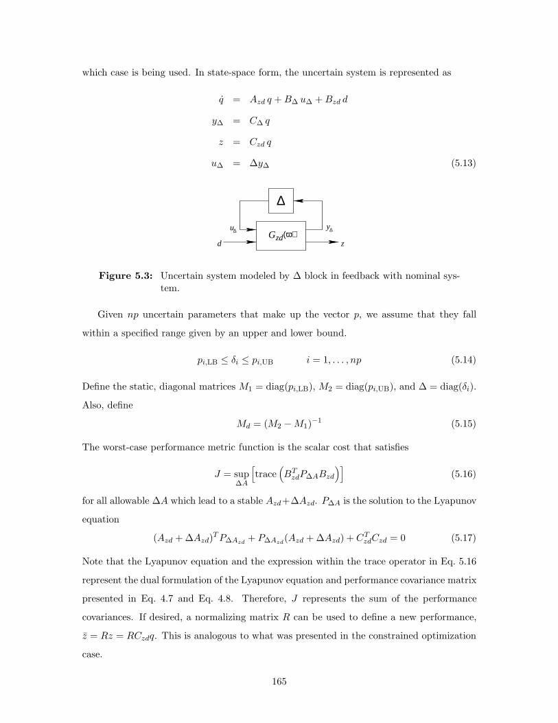
which case is being used. In state-space form, the uncertain system is represented as

q = Azd q +B∆ u∆ +Bzd d

y∆ = C∆ q

z = Czd q

u∆ = ∆y∆ (5.13)

G (ω)zdu∆

y∆

d z

∆

Figure 5.3: Uncertain system modeled by ∆ block in feedback with nominal sys-tem.

Given np uncertain parameters that make up the vector p, we assume that they fall

within a specified range given by an upper and lower bound.

pi,LB ≤ δi ≤ pi,UB i = 1, . . . , np (5.14)

Define the static, diagonal matrices M1 = diag(pi,LB), M2 = diag(pi,UB), and ∆ = diag(δi).

Also, define

Md = (M2 −M1)−1 (5.15)

The worst-case performance metric function is the scalar cost that satisfies

J = sup∆A

[trace

(BT

zdP∆ABzd

)](5.16)

for all allowable ∆A which lead to a stable Azd+∆Azd. P∆A is the solution to the Lyapunov

equation

(Azd + ∆Azd)TP∆Azd+ P∆Azd

(Azd + ∆Azd) + CTzdCzd = 0 (5.17)

Note that the Lyapunov equation and the expression within the trace operator in Eq. 5.16

represent the dual formulation of the Lyapunov equation and performance covariance matrix

presented in Eq. 4.7 and Eq. 4.8. Therefore, J represents the sum of the performance

covariances. If desired, a normalizing matrix R can be used to define a new performance,

z = Rz = RCzdq. This is analogous to what was presented in the constrained optimization

case.

165

Reference [37] uses Popov analysis and dissipation theory to derive the following robust

stability criterion. Given the system described by Eq. 5.11 with uncertainties specified by

Eq. 5.14, then if there exist diagonal matrices H > 0 and N ≥ 0, and if the following matrix

is positive definite

Ro = HMd +MdH −BT∆C

T∆N −NC∆B∆ (5.18)

then the system is robustly stable for all allowable ∆ provided that there is a matrix P ≥ 0

that solves the Riccati equation

(AT +CT∆R

−1o BT

∆)P+P (A+B∆R−1o C∆)+PB∆R

−1o BT

∆P+CTzdCzd+CT

∆R−1o C∆ = 0 (5.19)

where

A = Azd +B∆M1C∆

C∆ = HC∆ +NC∆A

In addition, a bound on the performance metric function J from Eq. 5.16 is given by

J ≤ J = trace[BT

zd(P + CT∆(M2 −M1)NC∆)Bzd

](5.20)

The matrices H and N are known as stability multipliers.

Reference [87] finds the minimum J by specifying an optimization problem which min-

imizes J with respect to the diagonal elements of H and N subject to the constraints

H > 0 and N ≥ 0. The SQP method is used to find a solution, and the gradient of J is

computed at each step. The Riccati equation constraint (Eq. 5.19) is implicitly accounted

for by computing the gradient of J only in directions that place the trial points within

the space defined by the Riccati equation. The positive definite constraint on the matrix

Ro is not included because it is felt that the Riccati equation will have no solution when

this constraint is not satisfied [87]. The optimization problem is shown to be convex, which

implies that a converged solution should theoretically represent the overall minimum.

Although this approach appears attractive because of the rigorous mathematical theory

that is used to derive the bound on J , it does suffer from a few disadvantages. One is that

only a bound is provided by the method. There is no indication of exactly how tight the

bound is. It also does not provide an estimate of the values δi of the ∆ block that produce

the bound. As a result, there is no way to estimate the individual worst-case performance

variances. Recall that J represents the sum of the performance variances. The previous two

166

methods yield both the separate variances and the worst-case uncertainties. This allows

the individual performance metrics to be compared against the requirements. Knowing the

worst-case parameter values enables the worst case to be checked by substituting the values

into the system and computing the performance.

When the system is written in structural modal form, theAzd matrix is of the form shown

in Eq. 4.41. For uncertainties in the open-loop damping ratios, the B∆ and C∆ matrices

can be created as follows. First consider the case of a single mode with the corresponding

A matrix

A =

0 1

−ω2 −2ζω

(5.21)

Assume the damping uncertainty is written as

ζ = ζo(1 + δ) (5.22)

This leads to

A =

0 1

−ω2 −2ζoω

+

0 0

0 −2ζoωδ

=

0 1

−ω2 −2ζoω

︸ ︷︷ ︸Ao

+

0

−2ζo

︸ ︷︷ ︸B∆

δ︸︷︷︸∆

[0 ω

]︸ ︷︷ ︸

C∆

(5.23)

Note that this is not a unique representation for B∆ and C∆ since −2ζoω can be broken

into two factors in several different ways.

For uncertainties in the open-loop natural frequencies, the procedure is not as direct.

The main difficulty can be seen by examining the single mode A matrix. The frequency

ω appears twice in the matrix. This would require ∆ to contain two diagonal elements;

however, there is no way to specify that the elements must be identical. This is due to the

fact that the stability multipliers H and N are restricted to be diagonal. Block diagonal

H and N would permit repeated elements in ∆. What is typically done in practice is to

assume uncertainty in the squared natural frequency (as is done in Reference [37]).

ω2 = ω2o(1 + δ) (5.24)

The uncertainty on ω is roughly δ/2. ∆A can be expressed as

B∆∆C∆ =

0

−ωo

δ [ ω 0

](5.25)

167

In general, if there is more than one uncertain frequency, then B∆ and C∆ can be

constructed as follows. Let ωi be the ith uncertain frequency, and assume that the ω2i term

appears at index (m,n) in the Azd matrix. Then the ith column of B∆ is

0...

0

−ωi

0...

0

← mth row (5.26)

and the ith row of C∆ is

[ 0 · · · 0 ωi 0 · · · 0 ]

↑ nth column(5.27)

In summary, this approach is appropriate to guarantee that the performance does not

exceed a bound. This bound is computed by solving a constrained optimization problem

with a Ricatti equation constraint and constraints on the stability multiplier matrices.

Unfortunately, it does not provide a sense of how close the bound is to the worst case, nor

does it indicate the values of the uncertain parameters that produce the bound.

5.3 Approximate Performance and Sensitivity Calculations

This section presents a model reduction technique that can be applied to large order state-

space models. The motivation is to reduce the computational expense in solving Lyapunov

equations. Performance assessment on a nominal state-space system involves determining

the state covariance matrix from Eq. 4.7. Section 4.2 showed that computing sensitivities

of performance covariances with respect to modal parameters involves solving a Lyapunov

equation for every performance metric. The solution represents the Lagrange multiplier

matrix that is required to compute the sensitivity. The order of a Lyapunov equation

equals the order of the state-space system. The goal is to reduce the size of the system while

maintaining the important dynamics. The approach is to determine a balanced realization

for the system, and then to reduce states which have small Hankel singular values.

168

5.3.1 Balanced model reduction

5.3.1.1 Balanced realization

The first step is to create a balanced realization of the state-space system. The tech-

nique is described in Reference [65]. The criterion for a “balanced” system is that both

the observability and controllability gramians are diagonal and equal. Consider again the

disturbance-to-performance system, which is repeated here.

q = Azd q +Bzd d

z = Czd q (5.28)

The observability gramian, Wo, is the solution to the Lyapunov equation

ATzdWo +WoAzd + CT

zdCzd = 0 (5.29)

while the controllability gramian, Wc, is the solution to the dual Lyapunov equation

AzdWc +WcATzd +BzdB

Tzd = 0 (5.30)

Note that Wc appears in an identical fashion as Σq in Eq. 4.7; hence, Wc is the state

covariance matrix in this case. In reality, Wc should be referred to as a disturbability

gramian since d is a disturbance and not a control input. However this distinction does not

affect the following steps.

We seek a similarity transformation matrix T such that when the states are transformed

via q = T q to produce the system

˙q = T−1AzdT︸ ︷︷ ︸Azd

q + T−1Bzd︸ ︷︷ ︸Bzd

d

z = CzdT︸ ︷︷ ︸Czd

q (5.31)

then the gramians of the transformed system satisfy

Wc = Wo = diagσ1, · · · , σn ≡ Σ (5.32)

The diagonal elements of Σ2 will be referred to as the gramian values, and their square

roots are known as the Hankel singular values [88]. It can be shown that

Wc = T−1WcT

Wo = T TWoT−1 (5.33)

169

The transformation matrix T and the Hankel singular values are obtained from the eigen-

value decomposition of the matrix WcWo.

WcWo = TΣ2T−1 (5.34)

The transformed states can be ordered such that the corresponding Hankel singular values

are in decreasing order. The relative sizes of the singular values provide an indication of

which states should be kept and which states might be eliminated. The intuition provided

by Hankel singular values is that since the observability and controllability gramians are

equal, large σ2i correspond to states that are highly observable and controllable (i.e., dis-

turbable). These states are typically quite visible in the various disturbance-to-performance

transfer functions. Because the system inputs are modeled with unit-intensity white-noise

disturbance processes, the performance metric variances can be thought of as the area under

the square of the transfer function magnitudes. Accurate performance prediction requires

these states be retained in the model.

5.3.1.2 Model truncation

The model reduction step begins by partitioning the states into those that will be kept, qk,

and those that will be removed, qr.

˙qk

˙qr

=

(Azd)kk (Azd)kr

(Azd)rk (Azd)rr

qk

qr

+

(Bzd)k

(Bzd)r

d

z =[

(Czd)k (Czd)r

]qk

qr

(5.35)

At this point, there are two popular options for removing the unwanted states qr. The

simplest involves truncating the state-space system as shown below.

˙qk = (Azd)kk qk + (Bzd)k d

z = (Czd)k qk (5.36)

However, this does not preserve the static gain of the transfer functions. If desired, a static

condensation procedure can be implemented as follows. First assume that the eliminated

states are infinitely fast, such that qr = 0. Eliminating qr from Eq. 5.35 results in the

170

following reduced system.

˙qk =[(Azd)kk − (Azd)kr(Azd)−1

rr (Azd)rk

]︸ ︷︷ ︸

Azd

qk +[(Bzd)k − (Azd)kr(Azd)−1

rr (Bzd)r]

︸ ︷︷ ︸Bzd

d

z =[(Czd)k − (Czd)r(Azd)−1

rr (Azd)rk

]︸ ︷︷ ︸

Czd

qk +[(Czd)r(Azd)−1

rr (Bzd)r]

︸ ︷︷ ︸Dzd

d (5.37)

This can be written in the standard form

˙q = Azd q + Bzd d

z = Czd q + Dzd d (5.38)

Notice that the static condensation method produces a D term which represents the static

gain of the reduced states. This feedthrough term causes the performance variables in z to

have infinite variance since the disturbance d is white noise. While Dzd helps the reduced

model at low frequencies, it does not permit the Gzd(ω) transfer function matrix to roll-off

at high frequencies. Thus, a way to remove Dzd while still preserving the low-frequency

behavior is desired.

5.3.1.3 Removal of D term

A common solution to this problem is to append high-frequency poles whose low-frequency

properties mimic that of the feedthrough term Dzd. At frequencies above the poles, there

will exist a natural roll-off at a rate related to the order of the pole. Various approaches

append the poles in different ways. For instance, the equivalent of a low-pass filter can

be placed between the actual white noise disturbance process d and a new disturbance d

which drives the system. Or the low-pass filter can be appended at the output such that

z represents the filtered response of the system. A faster roll-off in the filter comes at the

cost of more filter states, which increase the size of the system. Recall that the goal of

the current section is to examine ways to reduce the order of the state-space matrices. A

first-order roll-off in Gzd(ω) is sufficient to ensure a bounded performance covariance matrix

Σz.

To illustrate an approach for augmenting dynamics to remove Dzd, append Eq. 5.38

171

with a new system that represents the high frequency poles.

˙q

qa

︸ ︷︷ ︸

˙q

=

Azd 0

0 Aa

︸ ︷︷ ︸Azd

q

qa

︸ ︷︷ ︸

q

+

Bzd

Ba

︸ ︷︷ ︸Bzd

d

z =[Czd Ca

]︸ ︷︷ ︸

Czd

q

qa

(5.39)

Notice that theD term has purposely been set to zero in this appended system. The transfer

function matrix from d to z is given by

Gzd(s) = Czd(sI − Azd)−1Bzd + Ca(sI −Aa)−1Ba (5.40)

But the original transfer function matrix for the system described by Eq. 5.38 is of the form

Gzd(s) = Czd(sI − Azd)−1Bzd + Dzd (5.41)

Comparing Eq. 5.40 with Eq. 5.41 we see that the term Ca(sI − Aa)−1Ba appears in a

similar fashion as the term Dzd. Enforcing the constraint that the static gains for the two

systems be identical leads to the following relationship that must be satisfied

Dzd = Ca(−A−1a )Ba (5.42)

Let the dimension of Dzd be m × n. Performing a singular value decomposition on Dzd

leads to

Dzd = USV H (5.43)

Suppose that the rank of Dzd is r. Define the new matrices

U = first r columns of U

S = upper left r × r submatrix of S

V = first r columns of V

It is straightforward to show that

Dzd = U SV H (5.44)

where now S is an r× r positive-definite diagonal matrix. If −A−1a is also an r× r positive-

definite diagonal matrix, then Eq. 5.44 can be manipulated into the form

Dzd = U√S

√−A−1

a︸ ︷︷ ︸Ca

(−A−1a )

√−A−1

a

√SV H︸ ︷︷ ︸

Ba

(5.45)

172

The required matrices Ba and Ca can be identified by comparing Eq. 5.45 with Eq. 5.42.

What has not been discussed yet is how to specify Aa. The formulation above assumes that

Aa is a diagonal, negative-definite matrix. This can be achieved by augmenting the system

with r poles at a frequency of ωhi. Then Aa will be

Aa =

. . .

−ωhi

. . .

(5.46)

The poles are typically placed at frequencies a decade above the highest frequency that is

retained in the model.

5.3.1.4 Practical issues

A practical consideration when performing balanced model reduction is that if the various

input/output channels have different units, then the balanced realization will favor states

that are important in the transfer functions with larger magnitude. For example, suppose

that the system of interest is an interferometer, and one performance metric is optical

path difference (OPD) while another metric is wavefront tilt (WFT). If the OPD transfer

function is orders of magnitude larger than the WFT transfer function, then states that

are important to the WFT transfer function might have low Hankel singular values and be

reduced out. It is important to scale the system so that transfer functions of interest have

approximately the same magnitude level. (Recall that a numerical example of this issue

was provided in Section 3.3).

It is also known that the balanced reduction method is not optimal with respect to the

norm of the model error. The error is defined as the difference between the original transfer

function and the reduced transfer function (i.e., Gzd(ω)−Gzd(ω)). Nevertheless, the method

does provide a systematic approach to model reduction that can be easily implemented.

5.3.2 Analysis approximations during optimization iterations

When performing the uncertainty analysis via the constrained optimization approach de-

scribed previously, it is necessary to compute the cost J and its gradient ∂J∂p at each iteration

step. For systems with a very large number of states, each of these computations can re-

quire a significant amount of computation time. Ideally, a reduced model would be created

173

initially and then used for all subsequent computations. However, the parameters of inter-

est in the uncertainty analysis are open-loop modal parameters which appear explicitly in

the system Azd matrix (recall Eq. 4.41). The reduced Azd matrix, while smaller in size as

desired, has lost all explicit dependence on the modal parameters. Both the uncertainty

analysis and the sensitivity analysis (which is used to compute ∂J∂p ) require access to these

parameters. Figure 5.4 summarizes three possible options for model reduction during the

constrained optimization uncertainty analysis.

The initial solution to this problem is to perform a balanced model reduction at each

iteration step, as shown in the middle path in Figure 5.4(b). A new admissible set of

uncertain parameters is placed in Azd, and the reduction process described in the previous

section is applied to create Azd. The performance RMS values can then be obtained after

solving Eq. 4.7 and applying Eq. 4.8 for the reduced system. The drawback to this approach

is that determining the balancing transformation matrix T is the most time-consuming part

of the reduction process. For example, it required approximately 6.5 minutes on a Sun Ultra

1 to compute T for a model which has on the order of 300 states. The time saved by using a

reduced-order system in the Lyapunov equation, Eq. 4.7, is lost during the balancing step.

Performing balanced model reduction at each iteration, however, will not work when

computing the sensitivity ∂J∂p . As shown in Section 4.2, the expression for the sensitivity of

the cost J with respect to a parameter p is

∂J

∂p= trace

[L

(∂Azd

∂pΣq + Σq

∂ATzd

∂p

)](5.47)

where L is the Lagrange multiplier matrix and Σq is the state covariance matrix. It is

assumed that neither Bzd nor Czd is a function of p. The problem arises when computing∂Azd∂p and ∂AT

zd∂p . If the reduced matrix Azd is used, then these derivatives cannot be readily

computed.

A series of approximations is required to enable reduced-order models to be used during

the optimization routine. The first one addresses the issue of recomputing the balancing

transformation matrix T at each step. Let To be the transformation matrix that exactly

balances the original, unperturbed system. The assumption that is made is that for small

perturbations in the system, To will approximately balance the perturbed system. Con-

sidering only perturbations in the system Azd matrix leads to the following approximately

174

cost and sensitivity evaluation

SQP

converged?

converged?

SQP

zdA

C

Bzd

zd 0

*

perturbed, unreduced system

0

zdA

C

Bzd

zd

converged?

SQP

p(k+1) = p(k) + (k) d(k)α

zdA

C

Bzd

zd 0

*

perturbed, unreduced system

pworst-case

pworst-case pworst-case

p(k+1) = p(k) + (k) d(k)α

p(k+1) = p(k) + (k) d(k)α

J dJ/dp

dJ/dpJ

sensitivity evaluationapproximate cost and

reductionperform balanced model

use original T , elim_states

N

Y

N

YY

N

original, unreduced system

balancing transformation:states to reduce:

Telim_states

dJ/dpJ

sensitivity evaluationapproximate cost and

reductionperform balanced model

elim_statesT

(a) (b) (c)

zdA

C

Bzd

zd 0

*

perturbed, unreduced system

+ + +

compute , select

Figure 5.4: Model reduction options during constrained optimization uncertaintyanalysis. (a) No model reduction. (b) Exact balanced reduction ateach iteration. (c) Approximate balanced reduction at each itera-tion step. Both (b) and (c) rely on approximate cost and sensitivityevaluations.

175

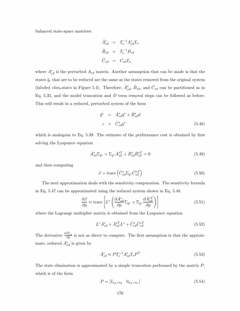
balanced state-space matrices:

A∗zd = T−1

o A∗zdTo

Bzd = T−1o Bzd

Czd = CzdTo

where A∗zd is the perturbed Azd matrix. Another assumption that can be made is that the

states qr that are to be reduced are the same as the states removed from the original system

(labeled elim states in Figure 5.4). Therefore, A∗zd, Bzd, and Czd can be partitioned as in

Eq. 5.35, and the model truncation and D term removal steps can be followed as before.

This will result in a reduced, perturbed system of the form

˙q∗ = A∗zdq

∗ + B∗zdd

z = C∗zdq

∗ (5.48)

which is analogous to Eq. 5.39. The estimate of the performance cost is obtained by first

solving the Lyapunov equation

A∗zdΣq∗ + Σq∗A

∗Tzd + B∗

zdB∗Tzd = 0 (5.49)

and then computing

J = trace(C∗

zdΣq∗C∗Tzd

)(5.50)

The next approximation deals with the sensitivity computation. The sensitivity formula

in Eq. 5.47 can be approximated using the reduced system shown in Eq. 5.48.

∂J

∂p≈ trace

[L∗(∂A∗

zd

∂pΣq∗ + Σq∗

∂A∗Tzd

∂p

)](5.51)

where the Lagrange multiplier matrix is obtained from the Lyapunov equation

L∗A∗zd + A∗T

zd L∗ + C∗

zdC∗Tzd (5.52)

The derivative ∂A∗zd

∂p is not as direct to compute. The first assumption is that the approxi-

mate, reduced A∗zd is given by

A∗zd ≈ PT−1

o A∗zdToP

T (5.53)

The state elimination is approximated by a simple truncation performed by the matrix P ,

which is of the form

P = [Ink×nk0nk×nr ] (5.54)

176

where nk is the number of states to keep and nr is the number to remove. The second

assumption is that To is not a function of the parameter p. This permits the derivative of

A∗zd to be expressed approximately as

∂A∗zd

∂p≈ PT−1

o

∂A∗zd

∂pToP

T (5.55)

The desired sensitivity is then computed by substituting ∂A∗zd

∂p , L∗, and Σq∗ into Eq. 5.51.

The validity of this approximation will be analyzed in the following section. The sequence

of steps that has just been outlined is shown in Figure 5.4(c).

5.4 Demonstration of Uncertainty Analysis

Having described a number of uncertainty analysis techniques and various approximations

that can be made, the next step is to apply the methodology to systems of increasing order.

The cases to be investigated are

• simple one degree-of-freedom (DOF) spring-mass system

• cantilevered beam with nearly square cross-section

• multiple DOF spring-mass system

• closed-loop model of the Space Interferometry Mission

The cantilevered beam example is used to motivate the need for a sophisticated uncertainty

analysis method for systems with high modal density.

5.4.1 Single DOF system

A classic spring-mass system with assumed modal damping will serve to demonstrate the

parametric uncertainty analysis. Figure 5.5(a) shows that the disturbance w is an inertial

force acting on the mass, and the performance metric z is the position of the mass. The

natural frequency is nominally 1 Hz. The disturbance is modeled as colored noise, which

means that it is the output of a linear shaping filter driven by unit-intensity, Gaussian

white noise. A sensitivity analysis on the nominal system yields the normalized sensitivi-

ties in Figure 5.5(b). The power spectral density of w is plotted in Figure 5.5(c). In this

example, the shaping filter is a first-order low pass filter with corner frequency at 1Hz.

177

Table 5.1: Uncertain parameters for single DOF case.

Parameter Nominal value Uncertainty Worst-case

ωn/2π 1Hz ±5% 0.95Hz (−5%)

ζ 0.01 ±10% 0.009 (−10%)

m 1 ±2% 0.98 (−2%)

A frequency-domain disturbance analysis produces the performance PSD in Figure 5.5(d).

The performance cumulative RMS plot indicates that the nominal performance RMS value

is 3.59 mm. A hypothetical performance requirement line at 1mm is also shown in Fig-

ure 5.5(d).

The three parameters that were considered uncertain are the modal frequency ωn, the

modal damping ζ, and the modal mass m. Table 5.1 lists the nominal values, the percent

uncertainties that were assumed, and the worst-case parameters identified during the un-

certainty analysis. Implementing the uncertainty analysis via the constrained optimization

approach produces the results in Figure 5.6. Ten separate runs were conducted, each with

a random initial guess for the uncertain parameters. Run 0 just shows the nominal pa-

rameter values (placed proportionally between the dotted lines representing the upper and

lower bounds). Each run converged to the lower uncertainty bound for each parameter.

This agrees with the intuition provided by the normalized sensitivities in Figure 5.5(b). All

the sensitivities are negative, which implies that decreasing the parameters will increase the

RMS. Lower damping results in a larger response magnitude. A lower natural frequency

keeps the mode away from the roll-off region of the disturbance filter, thereby exacerbating

the response. A lower modal mass allows the disturbance to excite the mode to a greater

extent. (Recall that q + 2ζωnq + w2n = w/m. As m decreases, the modal force increases.)

In this case, placing each parameter at the lower bound produces the largest RMS

increase. This is the same logic employed by the first-order approach. In fact, the first-

order approximation predicts a worst-case RMS of 4.20 mm (indicated by the dash-dot line

in Figure 5.6), which is in error by only −1.76% from the actual worst-case value of 4.27 mm.

Because of the system’s small number of states, the approximation techniques described

previously did not have to be applied. The exact cost and gradient information could be

provided to the Sequential Quadratic Programming method. Figure 5.7(a) shows that the

178

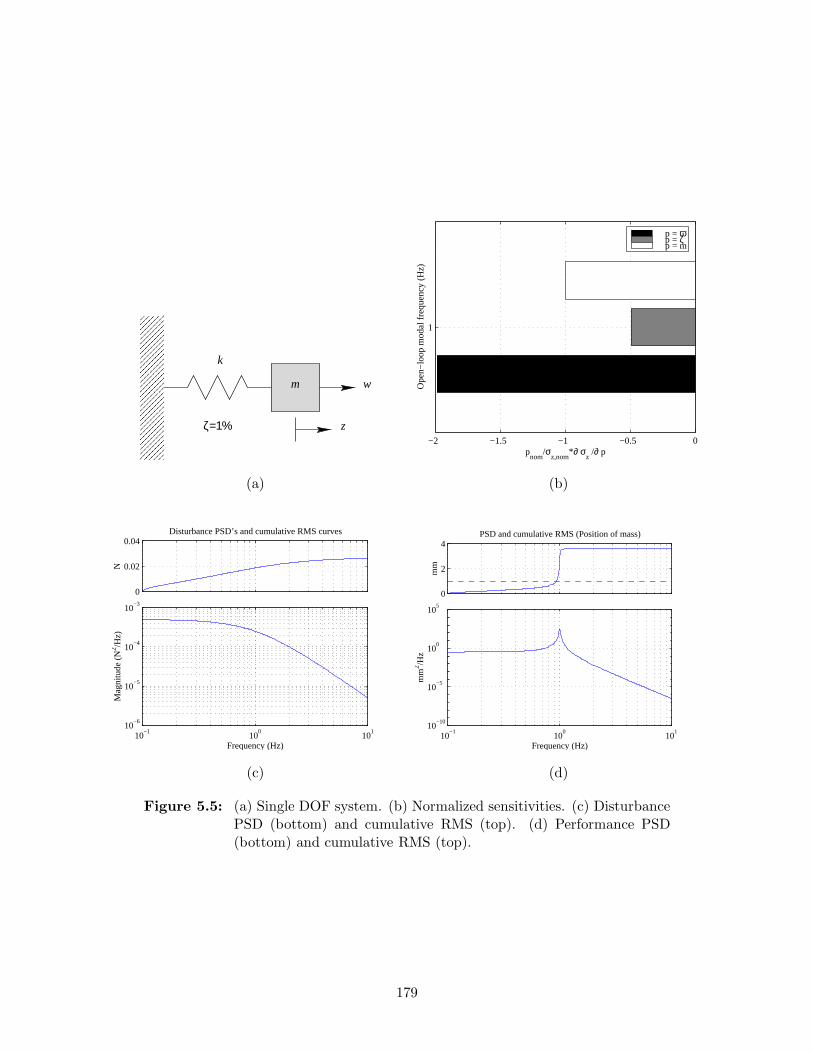
m w

zζ=1%

k

−2 −1.5 −1 −0.5 0

1

Ope

n−lo

op m

odal

freq

uenc

y (H

z)

pnom

/σz,nom

*∂ σz /∂ p

p = ωp = ζ p = m

(a) (b)

10−1

100

101

10−6

10−5

10−4

10−3

Frequency (Hz)

Mag

nitu

de (

N2 /Hz)

0

0.02

0.04Disturbance PSD’s and cumulative RMS curves

N

0

2

4

mm

PSD and cumulative RMS (Position of mass)

10−1

100

101

10−10

10−5

100

105

Frequency (Hz)

mm

2 /Hz

(c) (d)

Figure 5.5: (a) Single DOF system. (b) Normalized sensitivities. (c) DisturbancePSD (bottom) and cumulative RMS (top). (d) Performance PSD(bottom) and cumulative RMS (top).

179

0 1 2 3 4 5 6 7 8 9 10

1

2

3

Run #

Unc

erta

in p

aram

eter

#3

3.54

4.5

RM

S v

alue

(nm

)

Figure 5.6: Results of uncertainty analysis on single DOF case. Bottom plot,parameter values: Constrained optimization initial guess, , and con-verged solution, ∗. Parameter #1 = ωn, #2 = ζ, #3 = m. · · ·: upperor lower bound. Top plot, RMS values: −−− nominal; · · · initialguess; ∗ − ∗ worst case; − · − first-order approximation.

average time for the uncertainty analysis was on the order of 0.30 sec. Each of the ten runs

required only three iterations to converge to the worst-case parameters.

To examine the accuracy of the first-order approach, various levels of uncertainty were

assigned to the three modal parameters. The percent difference between the first-order

approach and the constrained optimization approach is plotted in Figure 5.7(b) as a function

of the uncertainty size. As expected, the first-order approximation produces negligible

errors only when the uncertainties are small. The approximation is no longer valid for large

uncertainty ranges.

In summary, it has been shown that for the case of a single mode driven by a low-

pass disturbance, the largest increase in performance RMS is accomplished by placing the

uncertain modal parameters at their lower bounds. The uncertainty analysis reveals that

the actual performance RMS can be as much as 19.0% larger than the nominal performance

for the uncertainty ranges considered.

180

0.28

0.3

0.32se

cTotal solution time

2

3

4

#

Number of iterations

1 2 3 4 5 6 7 8 9 100.08

0.1

0.12

sec

Average computation time per iteration

Run #10

−210

−110

010

110

210

−6

10−4

10−2

100

102

% Uncertainty

% d

iffer

ence

(a) (b)

Figure 5.7: (a) Time statistics for constrained optimization uncertainty analysis.(b) Percent differences between first-order approach and constrainedoptimization as a function of uncertainty size.

5.4.2 Cantilever beam

It is anticipated, however, that in general the worst-case parameters will not necessarily

be at the bound in the direction indicated by the sensitivity analysis. It can be envisioned

that for complex systems with high modal density, the results will not be as straightforward.

The coupling between parameters will not be negligible. An example of a cantilevered beam

with nearly repeated frequencies is used to demonstrate this fact.

Consider the beam depicted in Figure 5.8. The material is aluminum with density

2700 kg/m3, Young’s modulus 70 GPa, length 0.50 m and width 1 cm. Modal damping is

set to 0.5%. To cause the first two bending frequencies to almost coincide, let the height

of the beam be 1.05 cm. The disturbance is a tip force oriented at a 45 angle in the plane

of the cross-section. It is white noise with intensity 10−4 N2. The performance metric is

the tip displacement (in millimeters) along the same direction. The beam is modeled with

a single Bernoulli-Euler beam element with six DOF’s at the tip node. Furthermore, a

consistent mass matrix formulation is used. The first two frequencies are assumed to have

an uncertainty range of ±5%.

Figure 5.9(a) shows the tip displacement PSD for the nominal beam, as well as the PSD’s

for several combinations of uncertainties. Notice that the largest RMS value of the cases

shown corresponds to the case when the two frequencies happen to coincide at a frequency

equal to the geometric mean of the two nominal frequencies. This can be seen more clearly

181

F (white noise)

b

z

L

h

Figure 5.8: Cantilevered beam with nearly square cross-section.

in Figure 5.9(b), which zooms in on the region of interest.

The normalized sensitivities with respect to the nominal modal parameters of the first

four modes are presented in Figure 5.10(a). The largest sensitivities correspond to the

modal parameters of the first two modes. The signs indicate that to increase the RMS, these

parameters should be decreased. If the frequency parameters are placed at the uncertainty

bounds indicated by these sensitivities (i.e., at −5% and −5%, respectively), the resulting

RMS is not maximized. Thus a naıve guess which places the parameters at these bounds

does not capture the overall worst-case parameter variations.

Figure 5.11(a) shows the sensitivities with respect to the first two frequencies as the first

mode sweeps from −5% to +5% and the second mode sweeps from +5.3% to −4.8%. An

arbritary constraint that was imposed is that ω1ω1,nom

ω2ω2,nom

= 1, i.e., the geometric mean of

ω1 and ω2 is constant and equal to the nominal geometric mean of these two frequencies.

Because the uncertainty ranges of the two frequencies overlap, the sensitivity and perfor-

mance plots do not exhibit monotonic behavior in general. The frequency sensitivity curves

indicate that the slopes change sign twice during the frequency sweep. The performance

curves peak when the frequency ratio causes the two modes to coincide. This non-monotonic

phenomenon explains why relying solely on the nominal sensitivity information does not

work.

Placing the two frequencies at the geometric mean of the nominal frequencies has so far

been used only as a counter-example. It demonstrates that for the case of closely-spaced

modes, the worst-case performance does not necessarily occur when the uncertain modal

parameters are placed at one of their bounds. To find the true worst-case performance, the

uncertainty analysis optimization was applied to this beam example. Figure 5.12(a) shows

the results when the first two frequencies have a ±5% uncertainty. The second frequency

182

101

102

103

0

0.5

1

1.5R

MS

(m

m)

101

102

103

10−10

10−5

100

Frequency (Hz)

Mag

nitu

de (

mm2 /H

z)

±0% 2.47%, −2.41%−5%, −5% +5%, +5% −5%, +5% +5%, −5%

0

0.5

1

1.5

RM

S (

mm

)

33.87

10−4

10−2

100

Frequency (Hz)

Mag

nitu

de (

mm2 /H

z)(a) (b)

Figure 5.9: Tip displacement PSD’s and cumulative RMS curves for systems withvarious combinations of first and second mode frequencies. (a) Fullfrequency range. (b) Zoom around first two modes.

−1.5 −1 −0.5 0

33.06

34.71

325.7

342

Ope

n−lo

op m

odal

freq

uenc

y (H

z)

pnom

/σz,nom

*∂ σz /∂ p

p = ωp = ζ p = m

101

102

103

0

0.5

1

1.5

RM

S (

mm

)

101

102

103

10−10

10−5

100

Frequency (Hz)

Mag

nitu

de (

mm2 /H

z)

−5%, −5% −0.265%, −5%

(a) (b)

Figure 5.10: (a) Normalized sensitivities for the first four modes. (b) Tip displace-ment PSD’s and cumulative RMS curves for system with frequenciesplaced at lower bounds (−) and for system with frequencies specifiedby uncertainty analysis results (−−).

183

0.95 1 1.05

−10

0

10

Freq. ratio

Sen

sitiv

ity w

.r.t.

ω

0.95 1 1.05

1

1.1

1.2

1.3

Freq. ratio

RM

S (

nm)

0.95 1 1.05−0.3

−0.25

−0.2

Freq. ratio

Sen

sitiv

ity w

.r.t.

ζ

0.95 1 1.05−0.6

−0.55

−0.5

−0.45

−0.4

Freq. ratio

Sen

sitiv

ity w

.r.t.

m(a) (b)

Figure 5.11: Various plots obtained when ω1 (∗−∗) is swept up while ω2 (×−−×)is swept down. (a) Top: normalized sensitivity w.r.t. ω; bottom:performance RMS. (b) Top: normalized sensitivity w.r.t. ζ; bottom:normalized sensitivity w.r.t. m.

converges to the lower bound after each of the ten runs; however, the first frequency is not

as consistent. Runs 8 and 10 place the first frequency at its lower bound, but the RMS in

these runs clearly is not the worst-case value. Note also that the first-order approximation

(dashed-dot line) does poorly because it assumes the worst-case occurs at the uncertainty

bounds indicated by the sensitivities. It does approximate well the value obtained by the

two runs (8 and 10) that converged (incorrectly) to the lower bounds.

To provide a physical explanation for these results, consider the PSD and cumulative

RMS curves presented in Figure 5.10(b). The solid line corresponds to when the two

frequencies are placed at their lower bounds. We saw that this produced an RMS value

larger than any of the other cases which placed the frequencies at various combinations of

the bounds. The dashed line corresponds to placing the frequencies at the worst-case values

produced by the uncertainty optimization. The second frequency is located at its lower

bound (−5%), and the first frequency is placed at this same frequency. The cumulative

RMS curve indicates that this yields a slightly larger total RMS value.

Figure 5.12(b) shows the results when the damping ratios (uncertain parameters 3,4)

184

0 1 2 3 4 5 6 7 8 9 10

1

2

Run #

Unc

erta

in p

aram

eter

#

0.5

1

1.5R

MS

val

ue (

mm

)

0 1 2 3 4 5 6 7 8 9 10

1

2

3

4

5

6

Run #

Unc

erta

in p

aram

eter

#

0.5

1

1.5

RM

S v

alue

(m

m)

(a) (b)

Figure 5.12: Results of uncertainty analysis optimization after ten runs for beamwith closely-space modes. (a) Uncertainties only in frequencies offirst two modes. (b) Uncertainties in frequency, damping, and modalmass of first two modes.

and modal masses (uncertain parameters 5,6) of the first two modes are also treated as

uncertain. These parameters also converge to their lower bounds, which is consistent with

the negative sensitivities shown in Figure 5.10(a). The sensitivity plots in Figure 5.11(b) do

not exhibit monotonic behavior; however, they do not have rapid sign changes as was the

case for the sensitivity curve with respect to frequency. Since the sensitivities are always

negative, this could explain why the worst-case modal damping and mass parameters are

at the lower bounds.

Now we turn our attention to the case when the bending mode frequencies of the can-

tilevered beam are well separated. This is achieved by setting the height, h, of the beam to

1.8 cm. Figure 5.13(a) contains the tip displacement PSD’s and cumulative RMS curves for

the nominal system as well as for systems with the first two frequencies placed at various

uncertainty bounds. Because of the frequency separation, the uncertainty ranges do not

overlap. The largest RMS value corresponds to the case when the two frequencies are at

the lower bound of −5%. The sensitivities shown in Figure 5.13(b) confirm that the correct

direction to move the frequencies is toward the left (i.e., toward lower frequencies).

185

101

102

103

0

0.2

0.4R

MS

(m

m)

101

102

103

10−10

10−5

Frequency (Hz)

Mag

nitu

de (

mm2 /H

z)

±0% −5%, −5%+5%, +5%−5%, +5%+5%, −5%

−1.4 −1.2 −1 −0.8 −0.6 −0.4 −0.2 0

33.06

59.5

325.7

586.3

Ope

n−lo

op m

odal

freq

uenc

y (H

z)

pnom

/σz,nom

*∂ σz /∂ p

p = ωp = ζ p = m

(a) (b)

Figure 5.13: (a) Tip displacement PSD’s and cumulative RMS curves for systemswith various combinations of first and second mode frequencies. (b)Normalized sensitivities for the first four modes.

If we sweep the frequencies of the first and second modes in a similar fashion as was done

for the previous case, we obtain the sensitivity and performance curves shown in Figure 5.14.

All the curves are either monotonically increasing or decreasing. There are no drastic sign

changes as was seen before. This suggests that the worst-case parameter changes should be

at the bounds indicated by the signs of the sensitivities. To confirm this, the uncertainty

analysis optimization method was applied, and sample results are presented in Figure 5.15.

In most instances, all parameters converge to the lower bounds as expected. The cases in

which the optimization routine converged to a different solution have a lower RMS value,

and hence do not represent worst-case solutions.

Further work is needed to identify if in general for systems with adequate modal sep-

aration, the worst-case modal parameters will always lie at the appropriate uncertainty

bound. This would greatly simplify the uncertainty analysis since the computationally-

intensive optimization could be bypassed. Furthermore, this sample case showed that even

for closely-spaced modes, the sensitivities with respect to damping and modal mass did not

change sign over the uncertainty range. This suggests that the only parameters that might

be needed for the optimization method are the frequencies of the modes. Deriving general

186

0.95 1 1.05

−1.2

−1

−0.8

−0.6

−0.4

−0.2

Freq. ratio

Sen

sitiv

ity w

.r.t.

ω

0.95 1 1.050.41

0.42

0.43

0.44

0.45

Freq. ratio

RM

S (

nm)

0.95 1 1.05

−0.4

−0.3

−0.2

−0.1

Freq. ratio

Sen

sitiv

ity w

.r.t.

ζ

0.95 1 1.05

−0.8

−0.6

−0.4

−0.2

Freq. ratio

Sen

sitiv

ity w

.r.t.

m(a) (b)

Figure 5.14: Various plots obtained when ω1 (∗−−∗) is swept up while ω2 (×−×)is swept down. (a) Top: normalized sensitivity w.r.t. ω; bottom:performance RMS. (b) Top: normalized sensitivity w.r.t. ζ; bottom:normalized sensitivity w.r.t. m

0 1 2 3 4 5 6 7 8 9 10

1

2

Run #

Unc

erta

in p

aram

eter

#

0.4

0.45

0.5

RM

S v

alue

(m

m)

0 1 2 3 4 5 6 7 8 9 10

1

2

3

4

5

6

Run #

Unc

erta

in p

aram

eter

#

0.4

0.45

0.5

RM

S v

alue

(m

m)

(a) (b)

Figure 5.15: Results of uncertainty analysis optimization after ten runs for beamwith well-separated modes. (a) Uncertainties only in frequencies offirst two modes. (b) Uncertainties in frequency, damping, and modalmass of first two modes.

187

results such as this would be highly beneficial, and efforts in this area should be pursued.

5.4.3 Multi-DOF system

Now consider the system in Figure 5.16(a) consisting of 20 masses and 19 springs. Each

mass and spring constant was randomly selected from a specified interval. Modal damp-

ing was uniformly assigned a value of 0.1%. There are a total of six disturbance input

locations at DOF’s 7 through 12. The performance metric is the differential motion of the

two end masses (i.e., z = x20 − x1). The PSD’s of the disturbances are shown in Fig-

ure 5.16(b), where the larger magnitude PSD corresponds to the first three disturbances

and the lower magnitude PSD corresponds to the last three disturbances. Propagating

these PSD’s through the system disturbance-to-performance transfer function yields the

performance PSD in Figure 5.16(c). Three modes contribute most to the RMS value, as

indicated by the cumulative RMS curve. The normalized sensitivities with respect to the

modal parameters of these modes are indicated in Figure 5.16(d).

At this point, it is useful to comment on the importance of the information provided

by the sensitivity analysis and the frequency-domain disturbance analysis. Both can be

used to identify the dominant system modes. When performing an uncertainty analysis,

only uncertainties in parameters associated with these modes need to be considered. The

uncertainties in the other modes have to be extremely large to affect the performance

in a comparable manner as the uncertainties in the critical modes. Therefore, these two

analyses can reduce the total number of uncertain parameters that are carried through to

the uncertainty analysis. Although all modes might initially be considered uncertain to

some degree, only a subset will be important. In this case, the modal parameters of the

first three modes are treated as uncertain. This yields a total of nine uncertain parameters.

The nominal uncertainties are shown in Table 5.2.

The multi-DOF model is useful in showing the benefits of using reduced models and

of supplying the optimization routine with gradient information. The model is of a size

which permits some of these issues to be explored. First, consider the efficiency of the

SQP routine when it has knowledge of the gradients of the cost function. Figure 5.17(a)

displays the results of ten runs of the uncertainty analysis when analytical gradients are not

provided. Only one run (#9) comes closest to converging to the proper bounds. One reason

for this could be that when gradients are not supplied, the MATLAB function constr.m

188

x1

1m

ζ=0.1%

kkkk1

2x

m2

2

m

x

m

x

19

18

19

19

20

20

(a)

101

102

103

10−6

10−5

10−4

10−3

10−2

Frequency (Hz)

Mag

nitu

de (

N2 /Hz)

0

0.5

1

1.5Disturbance PSD’s and cumulative RMS curves

N

0

5

10

nm

Performance PSD and cumulative RMS curve

101

102

103

10−15

10−10

10−5

100

105

Frequency (Hz)

Mag

nitu

de (

nm2 /H

z)

(b) (c)

−1 −0.9 −0.8 −0.7 −0.6 −0.5 −0.4 −0.3 −0.2 −0.1 0

47.81

83.55

110.8

Normalized sensitivities

Ope

n−lo

op m

odal

freq

uenc

y (H

z)

pnom

/σz,nom

*∂ σz /∂ p

p = ωp = ζ p = m

(d)

Figure 5.16: (a) 20 DOF spring/mass system. (b) Disturbance PSD’s (bottom)and cumulative RMS (top). (c) Performance PSD (bottom) and cu-mulative RMS (top). (d) Normalized sensitivities of critical modes.

189

Table 5.2: Uncertain parameters for multi-DOF case.

# Parameter Nominal value Uncertainty

1 ω1/2π 47.8Hz ±5%

2 ω2/2π 83.5Hz ±5%

3 ω3/2π 110.8Hz ±5%

4 ζ1 0.01 ±10%

5 ζ2 0.01 ±10%

6 ζ3 0.01 ±10%

7 m1 1 ±2%

8 m2 1 ±2%

9 m3 1 ±2%

uses a finite-difference approximation. Section 4.4.2 showed that for this model, the finite-

difference approximation can contain significant errors as the perturbation size is made

extremely small. Figure 5.17(b) shows the results when the same initial guesses are used

in the ten runs, but this time the analytical gradients are computed. All runs consistently

converge to the lower bounds of the parameters. In addition, Figure 5.18(a) indicates that

the computation time is improved by factors of 5–10.

The first-order approximation is expected to do best when the uncertainty ranges are

small, and this is confirmed in Figure 5.18(b). The uncertainty size is assumed to be the

same for all nine parameters, and this size takes on the values ±10%, ±1%, and ±0.1%.

As Figure 5.18(b) shows, the percent difference between the worst case predicted by the

first-order approach and the worst case predicted by the optimization becomes smaller as

the uncertainty size is reduced.

The advantages of using reduced-order models can be demonstrated by considering a

series of reduced models with the number of states equal to 36, 28, 22, and 18, respectively.

The balanced model reduction method described in the previous section was used, and

the performance PSD plot for these different size models can be found in Figure 5.19(a).

Also shown is the cumulative RMS plot, which indicates that all models predict essentially

the same overall RMS value. Although significant differences can be seen in the PSD’s,

particularly at low and high frequencies, all the various size models accurately capture the

190

0 1 2 3 4 5 6 7 8 9 10

1

2

3

4

5

6

7

8

9

Run #

Unc

erta

in p

aram

eter

#

8

10

12R

MS

val

ue (

nm)

0 1 2 3 4 5 6 7 8 9 10

1

2

3

4

5

6

7

8

9

Run #

Unc

erta

in p

aram

eter

#

8

10

12

RM

S v

alue

(nm

)

(a) (b)

Figure 5.17: Results of uncertainty analysis optimization after ten runs. (a) Full-order model without gradient calculations. (b) Full-order model withgradient calculations.

behavior in the frequency range of the dominant modes. When performing model reduction,

it is important to confirm that the reduced model still contains the necessary dynamics for

accurate performance prediction.

Figure 5.19(b) plots the gramian values of the balanced, full-order system, and they are

normalized such that the largest has a value of 1. They are sorted in decreasing size, and

there are a total of 42 since the system has 42 states. Immediately, one notices that the last

four states can be reduced out because their gramian values are several orders of magnitude

smaller than the ones preceding them. Reducing out more states is then a trade-off between

smaller-order models and performance prediction capability.

The main advantage of smaller-order models is that the time to solve Lyapunov equations

is reduced. When performing the uncertainty analysis optimization, time savings at each

iteration manifests itself as overall time savings in the solution process. This is evident

in Figure 5.20(a), which shows the total solution time, the total number of iterations,

and the computation time per iteration for each run of the optimization. Gradient (i.e.,

sensitivity) information is computed at each iteration, which implies that the solution of an

191

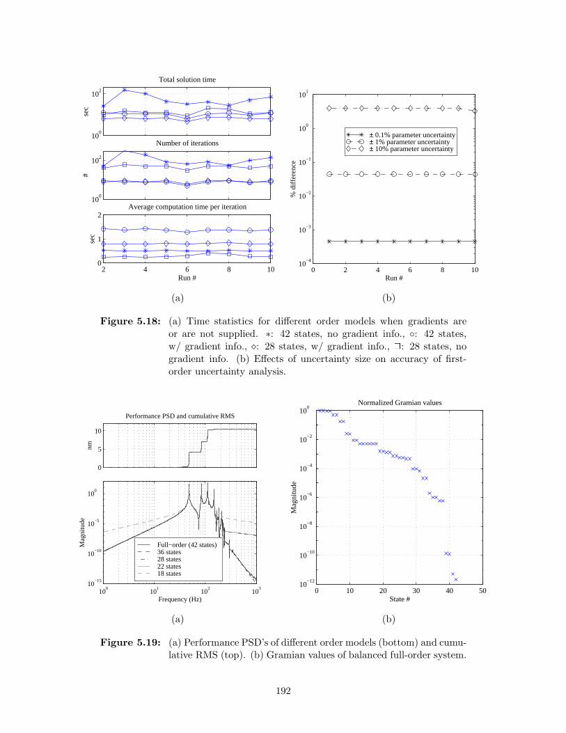
100

102

sec

Total solution time

100

102

#

Number of iterations

2 4 6 8 100

1

2

sec

Average computation time per iteration

Run #0 2 4 6 8 10

10−4

10−3

10−2

10−1

100

101

Run #

% d

iffer

ence

± 0.1% parameter uncertainty± 1% parameter uncertainty ± 10% parameter uncertainty

(a) (b)

Figure 5.18: (a) Time statistics for different order models when gradients areor are not supplied. ∗: 42 states, no gradient info., : 42 states,w/ gradient info., : 28 states, w/ gradient info., 2: 28 states, nogradient info. (b) Effects of uncertainty size on accuracy of first-order uncertainty analysis.

100

101

102

103

10−15

10−10

10−5

100

Frequency (Hz)

Mag

nitu

de

0

5

10

nm

Performance PSD and cumulative RMS

Full−order (42 states)36 states 28 states 22 states 18 states

0 10 20 30 40 5010

−12

10−10

10−8

10−6

10−4

10−2

100

State #

Mag

nitu

de

Normalized Gramian values

(a) (b)

Figure 5.19: (a) Performance PSD’s of different order models (bottom) and cumu-lative RMS (top). (b) Gramian values of balanced full-order system.

192

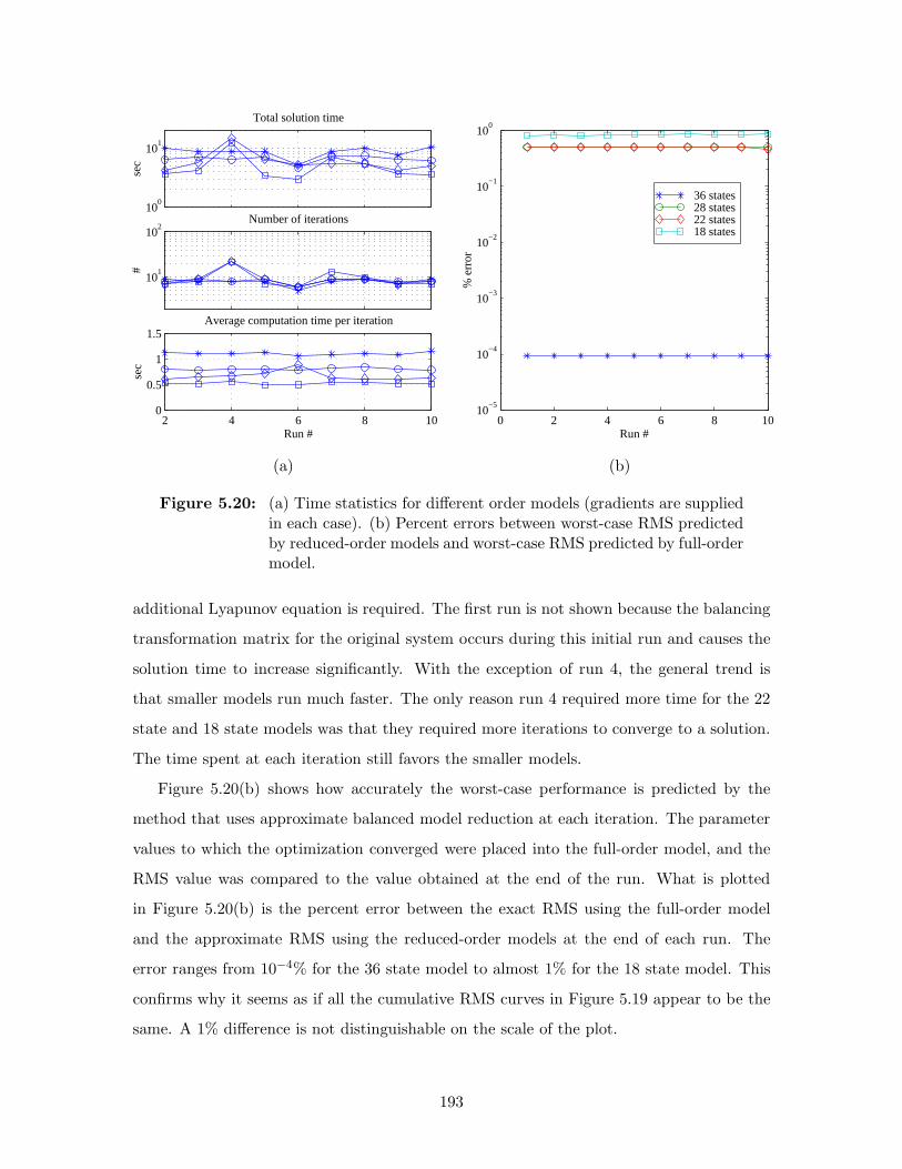
100

101

sec

Total solution time

101

102

#

Number of iterations

2 4 6 8 100

0.5

1

1.5

sec

Average computation time per iteration

Run #0 2 4 6 8 10

10−5

10−4

10−3

10−2

10−1

100

Run #

% e

rror

36 states28 states22 states18 states

(a) (b)

Figure 5.20: (a) Time statistics for different order models (gradients are suppliedin each case). (b) Percent errors between worst-case RMS predictedby reduced-order models and worst-case RMS predicted by full-ordermodel.

additional Lyapunov equation is required. The first run is not shown because the balancing

transformation matrix for the original system occurs during this initial run and causes the

solution time to increase significantly. With the exception of run 4, the general trend is

that smaller models run much faster. The only reason run 4 required more time for the 22

state and 18 state models was that they required more iterations to converge to a solution.

The time spent at each iteration still favors the smaller models.

Figure 5.20(b) shows how accurately the worst-case performance is predicted by the

method that uses approximate balanced model reduction at each iteration. The parameter

values to which the optimization converged were placed into the full-order model, and the

RMS value was compared to the value obtained at the end of the run. What is plotted

in Figure 5.20(b) is the percent error between the exact RMS using the full-order model

and the approximate RMS using the reduced-order models at the end of each run. The

error ranges from 10−4% for the 36 state model to almost 1% for the 18 state model. This

confirms why it seems as if all the cumulative RMS curves in Figure 5.19 appear to be the

same. A 1% difference is not distinguishable on the scale of the plot.

193

0 1 2 3 4 5 6 7 8 9 10

1

2

3

4

5

6

7

8

9

Run #

Unc

erta

in p

aram

eter

#

8

10

12R

MS

val

ue (

nm)

0 1 2 3 4 5 6 7 8 9 10

1

2

3

4

5

6

7

8

9

Run #

Unc

erta

in p

aram

eter

#

8

10

12

RM

S v

alue

(nm

)

(a) (b)

Figure 5.21: Results of uncertainty analysis optimization after ten runs. (a)Reduced-order model (28 states) without gradient calculations. (b)Reduced-order model (28 states) with gradient calculations.

Figure 5.21 shows the uncertainty analysis plots obtained after running the optimization

routine ten times for the 28 state reduced model. Subplot (a) is for the case when gradients

are not computed analytically at each iteration, while subplot (b) is for the case when the

gradients are computed. The same initial guesses were provided to the corresponding runs

of both cases. As can be seen, both cases converged to the lower bound of all the uncertain

modal parameters. The time statistics for each of the runs can be found in Figure 5.18(a),

and the benefits of knowing the gradients at each iteration are evident. Although the

computation time per iteration becomes larger when gradients are computed, the savings

are achieved because gradient information helps convergence to occur in a fewer number of

iterations.

At this point, we can examine the validity of the approximation methods that were

applied. Recall that one approximation is that the balancing transformation matrix of the

original, unreduced system will also approximately balance the perturbed system. Fig-

ure 5.22(a) compares the exact gramian values of the balanced, perturbed system with the

diagonal entries of the controllability gramian for the perturbed system after it has been

194

5 10 15 20 25 30 35 40

10−10

10−5

100

State #

Mag

nitu

de

Approx.Exact

1 2 3 4 5 6 7 8 910

−4

10−3

10−2

10−1

100

101

Parameter #

% e

rror

18 states, condensed22 states, condensed28 states, condensed36 states, condensed18 states, truncated22 states, truncated28 states, truncated36 states, truncated

(a) (b)

Figure 5.22: (a) Gramian values of exactly balanced system and approximatelybalanced system. Values shown are for one specific iteration dur-ing uncertainty optimization run. (b) Average error in approximatesensitivity computation during uncertainty optimization run.

transformed. In other words, let To be the original transformation matrix. The control-

lability gramian for the perturbed system after it has been transformed using To will not

necessarily be diagonal. Figure 5.22(a) plots the diagonal entries of this controllability

gramian matrix along with the exact gramian values. There are only minor differences in

the magnitude of the two different sets of values. It is anticipated that the differences would

be more apparent if the system was perturbed in a much larger fashion than it was for this

demonstration case.

Figure 5.22(b) provides an indication of the error in the approximate sensitivity com-

putations for the different size models. It shows for each of the nine uncertain modal

parameters the average percent error in the sensitivities with respect to those parameters.

In general, the sensitivities are more accurate when the model is not reduced drastically.

Also, it appears as if the sensitivities are more accurate when the model is reduced by a

strict truncation instead of by a static condensation. The only exception is for some of the

parameters of the model with 36 states.

To summarize, the multiple mass-spring model has served to identify some of the impor-

195

tant issues regarding model reduction in the uncertainty analysis optimization technique.

The lesson learned is that care must be taken in reducing the state-space system to the

appropriate size to gain the benefits of faster computation time while still preserving the

accuracy of the approximate cost and sensitivity estimates. In addition, the use of the

original balancing transformation matrix during all of the iterations appears to be valid in

this case.

5.4.4 SIM Classic

The integrated model of SIM Classic will now be used to demonstrate the uncertainty anal-

ysis technique on a system with an even larger number of states. Figure 5.23(a) shows the

finite-element model and a ray trace of stellar light passing through two arms of guide inter-

ferometer #1. The model is identical to the one used in the frequency-domain disturbance

analysis described in Section 3.3. The disturbance PSD’s are obtained from a low-order

shaping filter that approximates the PSD’s of a four-wheel configuration of Hubble-class

reaction wheels whose speeds are treated as uniform random variables over the range 0–

3000 RPM. (A description of the shaping filter was provided in Section 4.4.3.)

The performance metric for this example is the total stellar optical path difference

(OPD) of the guide interferometer visible in Figure 5.23(a). The PSD and cumulative RMS

curve of the OPD when the disturbances are propagated through the SIM model are shown

in Figure 5.23(c). The dominant modes are in the 10–20 Hz range as is indicated by the

sharp vertical steps in the cumulative RMS curve across these frequencies. The normalized

sensitivities of this RMS value with respect to the modal parameters of three of the most

dominant modes are presented in Figure 5.23(d). The frequencies have positive sensitivities,

and this implies that the worst-case RMS should be obtained when the modal frequencies

are increased.

The disturbance and sensitivity analysis results in Figure 5.23 were used to select three

critical modes for the uncertainty analysis. Initially, only the frequencies of these modes were

considered to be uncertain. The frequencies and uncertainty values are listed in Table 5.3.

The results of ten runs of the uncertainty analysis using the constrained optimization ap-

proach are shown in the usual form in Figure 5.24. The left subplot truncates the model

to 150 states at each iteration in order to perform the approximate sensitivity performance

evaluations. The right subplot truncates the model to 120 states. With the exception of

196

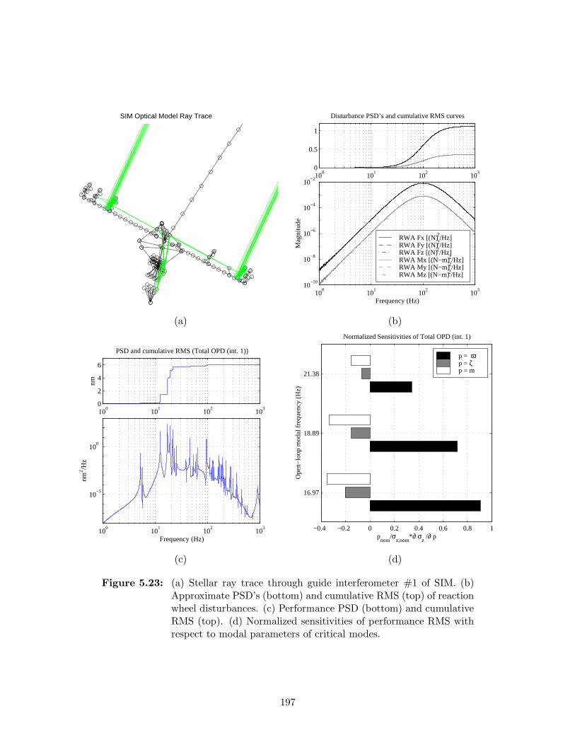
SIM Optical Model Ray Trace

100

101

102

103

0

0.5

1

Disturbance PSD’s and cumulative RMS curves

100

101

102

103

10−10

10−8

10−6

10−4

10−2

Frequency (Hz)M

agni

tude

RWA Fx [(N)2/Hz] RWA Fy [(N)2/Hz] RWA Fz [(N)2/Hz] RWA Mx [(N−m)2/Hz]RWA My [(N−m)2/Hz]RWA Mz [(N−m)2/Hz]

(a) (b)

100

101

102

103

0

2

4

6

nm

PSD and cumulative RMS (Total OPD (int. 1))

100

101

102

103

10−5

100

Frequency (Hz)

nm2 /H

z

−0.4 −0.2 0 0.2 0.4 0.6 0.8 1

16.97

18.89

21.38

Normalized Sensitivities of Total OPD (int. 1)

Ope

n−lo

op m

odal

freq

uenc

y (H

z)

pnom

/σz,nom

*∂ σz /∂ p

p = ωp = ζ p = m

(c) (d)

Figure 5.23: (a) Stellar ray trace through guide interferometer #1 of SIM. (b)Approximate PSD’s (bottom) and cumulative RMS (top) of reactionwheel disturbances. (c) Performance PSD (bottom) and cumulativeRMS (top). (d) Normalized sensitivities of performance RMS withrespect to modal parameters of critical modes.

197

the first run, the 150 state case consistently converges to the upper bound of the modal

frequencies. The reduced-order models only slightly underpredict the worst-case perfor-

mance achieved when the upper bounds are placed into the full-order model and the exact

RMS is computed. The first-order sensitivity approach does a good job, although it also

underpredicts. The average time required to complete an iteration of the optimization was

46.6 sec, and the average number of iterations before a run would converge was 6. Thus, a

typical run would only require less than five minutes to arrive at a prediction of the worst-

case performance. The final result of this case indicates that with ±5% uncertainty in the

frequencies of three critical modes, the predicted RMS value can increase from its nominal

value of 5.57 nm to a worst-case value of 6.37 nm, which represents a 14.4% increase.

For the 120 state case, the reduced-order model has a larger error in its ability to

predict the actual performance; consequently, the optimization routine has more difficulty

in converging to the correct parameter bounds. This reveals the importance of choosing

the correct size for the reduced-order model. A plot of the gramian values in Figure 5.25

indicates that the value of the 150th gramian is a factor of 10 lower than the value of the

120th gramian. Since it is not readily apparent based on this plot that the 150 state model

should do significantly better than a 120 state model, several model reduction iterations

are needed to ensure that the reduced model has retained a sufficient number of states for

performance prediction.

Now consider the situation when we treat as uncertain all the modal parameters as-

sociated with the three dominant modes. The pertinent values are listed in Table 5.3.

Figure 5.26 shows the outcome of ten runs of the optimization routine. Most runs consis-

tently place the frequencies at the upper bounds and the damping at the lower bounds. The

seven runs that produce the largest RMS (as predicted by the reduced model) place the

second and third modal masses at the lower bounds and the first modal mass at the upper

bound. This first modal mass is the only parameter that converges to a bound different from

that indicated by the sign of the sensitivity. Upon closer examination, run 3 does place the

first modal mass at the lower bound. This particular case shows that the RMS predicted

by the full-order model (indicated by a 2) is slightly larger than the RMS predicted by

the corresponding reduced-order model. These results lead to a possible conclusion that

the model reduction is not accurately capturing the true RMS level. This highlights the

need for proper model reduction, and the example is meant to demonstrate the results from

198

Table 5.3: Uncertain parameters for SIM case.

# Parameter Nominal value Uncertainty

1 ω13/2π 16.97Hz ±5%

2 ω15/2π 18.89Hz ±5%

3 ω17/2π 21.38Hz ±5%

4 ζ1 0.001 ±10%

5 ζ2 0.001 ±10%

6 ζ3 0.001 ±10%

7 m1 1 ±2%

8 m2 1 ±2%

9 m3 1 ±2%

0 1 2 3 4 5 6 7 8 9 10

1

2

3

Run #

Unc

erta

in p

aram

eter

#

5

6

7

RM

S v

alue

(nm

)

0 1 2 3 4 5 6 7 8 9 10

1

2

3

Run #

Unc

erta

in p

aram

eter

#

5

6

7

RM

S v

alue

(nm

)

(a) (b)

Figure 5.24: (a) Uncertainty analysis runs when SIM model is reduced to 150states at each iteration. (b) Uncertainty analysis runs when SIMmodel is reduced to 120 states at each iteration. Both plots: ,initial guess; ∗, converged solution; · · ·, upper or lower bound; −−−,nominal; 2, exact; − · −, first-order approximation.

199

0 50 100 150 200 250 300 35010

−12

10−10

10−8

10−6

10−4

10−2

100

State #

Mag

nitu

de

Normalized Gramian values

Figure 5.25: Gramian values of SIM model.

a “poor” uncertainty analysis. If a situation such as this was found to be the case, then

another series of runs would have to be done.

5.5 Summary

A methodology has been developed that predicts the worst-case RMS values of a system’s

performance metrics. The worst-case RMS arises due to parametric uncertainties in a

state-space model of the system. Initial work has considered the special case when the

uncertainties are in the open-loop modal parameters, and the uncertainties are specified as

bounds on these parameters. The methodology solves a constrained optimization problem,

and it does not assume that the worst-case parameters occur at their bounds. As a result, it

can accommodate cases in which the sensitivities change sign across the uncertainty range.

This can arise, for example, when the modal separation is smaller than the uncertainty

in the frequencies. Since the disturbances are modeled by filters that shape white noise,

it is possible to compute exact sensitivities (i.e., gradients) at each iteration of the opti-

mization. Gradient information helps the optimization converge more efficiently. When the

system has a significant number of states, an approximate balanced model reduction is per-

formed. Instead of computing the exact balancing transformation matrix at each iteration,

which is a time-consuming process, the original balancing transformation matrix is used.

Approximate RMS and sensitivity values can then be computed. The methodology has

200

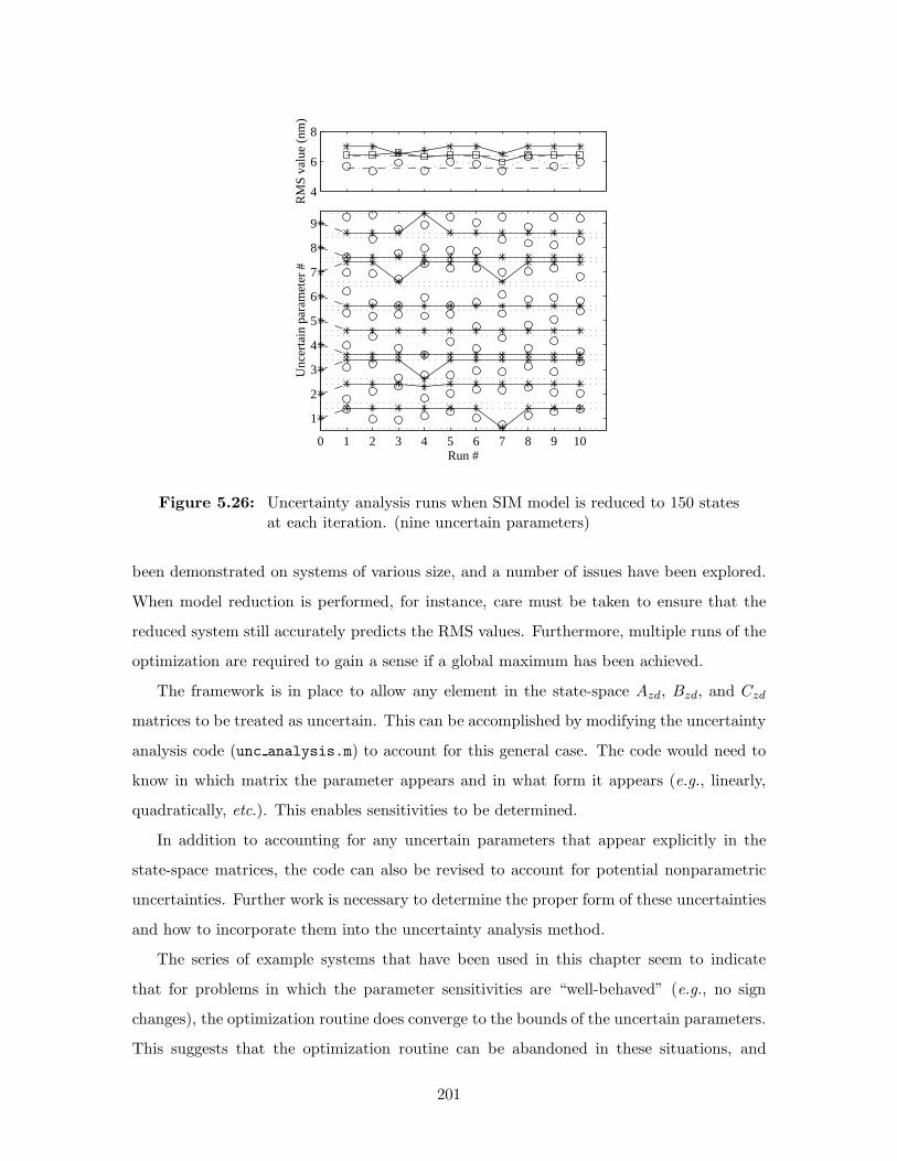
0 1 2 3 4 5 6 7 8 9 10

1

2

3

4

5

6

7

8

9

Run #

Unc

erta

in p

aram

eter

#

4

6

8

RM

S v

alue

(nm

)

Figure 5.26: Uncertainty analysis runs when SIM model is reduced to 150 statesat each iteration. (nine uncertain parameters)

been demonstrated on systems of various size, and a number of issues have been explored.

When model reduction is performed, for instance, care must be taken to ensure that the

reduced system still accurately predicts the RMS values. Furthermore, multiple runs of the

optimization are required to gain a sense if a global maximum has been achieved.

The framework is in place to allow any element in the state-space Azd, Bzd, and Czd

matrices to be treated as uncertain. This can be accomplished by modifying the uncertainty

analysis code (unc analysis.m) to account for this general case. The code would need to

know in which matrix the parameter appears and in what form it appears (e.g., linearly,

quadratically, etc.). This enables sensitivities to be determined.

In addition to accounting for any uncertain parameters that appear explicitly in the

state-space matrices, the code can also be revised to account for potential nonparametric

uncertainties. Further work is necessary to determine the proper form of these uncertainties

and how to incorporate them into the uncertainty analysis method.

The series of example systems that have been used in this chapter seem to indicate

that for problems in which the parameter sensitivities are “well-behaved” (e.g., no sign

changes), the optimization routine does converge to the bounds of the uncertain parameters.

This suggests that the optimization routine can be abandoned in these situations, and

201

only a single disturbance analysis has to be conducted on the system after placing the

parameters at the bounds that lie in the directions indicated by the sensitivities. If such a

generalization can be proved mathematically rather than assumed from heuristic arguments,

then this would constitute a significant contribution. Efforts in this area are recommended.

Furthermore, there are additional indications that even for poorly-behaved sensitivities

with respect to frequencies, the sensitivities with respect to modal mass and damping

never experience sign changes. This was seen in the cantilevered beam example. If this

can be shown in general, then the only parameters that would have to be considered in

the optimization routine are the uncertain frequencies. Once the worst-case frequencies

are determined, then the uncertain damping and modal mass values can be placed at the

appropriate bounds (which are usually the lower ones).

202

Chapter 6

Experimental Validation

The theory behind a series of analysis tools has been described in the preceding chapters.

In particular, the framework for determining the sensitivity of performance RMS values

with respect to physical parameters appears to be a promising design aid. It has been

demonstrated on systems ranging from a cantilever beam to a closed-loop integrated model

of SIM Classic; however, the key to using it with confidence is to successfully validate it in

practice. Further demonstration of the code on other purely analytical systems would still

not address the issue of its applicability in a real-world setting. As a result, a laboratory

testbed was designed and constructed to help identify potential limitations that were not a

factor during analytical simulations.

This chapter begins by describing the requirements that were placed on the testbed

before the design process began. The task of meeting the requirements subject to material

and time constraints led to a point design which consists of a cantilevered truss with a flexible

appendage. The details of this design are provided, and this is followed by an overview of

the initial finite-element model that was created in IMOS. After this, a technique to update

FEM parameters based on measured transfer functions is implemented. The results of a

series of experimental tests are then shown and compared to the analytical predictions made

using the updated model. An example design problem concludes the chapter by illustrating

in both theory and practice how the physical parameter sensitivities can identify redesigns

that improve the performance.

203

6.1 Description of Testbed

One of the top-level requirements placed on the testbed was that it must be able to address

two research topics. Its primary role is to serve as a sensitivity analysis validation platform.

Its other role is to serve as a testbed for research in reaction wheel disturbance modeling.

The implications of these criteria are evident in the desired testbed characteristics listed in

Table 6.1. Due to constraints on time and cost, the testbed had to be constructed from as

much available hardware as possible and with a minimal amount of newly machined parts.

Several dozen aluminum struts and node balls were obtained from a previous experiment

and used as the basic components of the testbed. A cantilevered, truss-like configuration

was chosen since it was of medium complexity. A view of the overall testbed is provided

in Figure 6.1(a). A more complicated structure would have required more time for con-

struction. In addition, modeling a complex structure would possibly have introduced large

errors that would have masked the issues of interest. On the other extreme, a less complex

structure would not have been as traceable, even if successful experimental results were

obtained.

The hole pattern in the node balls allows truss configurations with either triangular

or square cross sections, and the triangular arrangement was selected since it minimizes

the number of nodes and struts for a structure of a given length. Each bay of the truss

consists of an inverted, square-based pyramid whose apex is connected to the apexes of

neighboring bays by two struts. A plate can be easily added to the square top of any bay,

and a disturbance source such as a reaction wheel can be attached to the plate. The truss

was placed horizontally on an optics table to permit easy access to any bay. This is essential

since sensitivity validation requires repeated modifications to the structure. The base of

the truss consists of a pattern of nodes and struts that allows the truss to be attached to

the optics table at four node locations.

During the course of the SIM physical parameter sensitivity analysis in Section 4.6.2, it

was discovered that the critical modes consisted of a global mode and two local siderostat

bay modes. To introduce a local mode to the testbed that was close in frequency to the

truss primary bending modes, a flexible appendage was added at the end of the truss,

and it can be seen clearly in Figure 6.1(b). Ideally, it was desired that the testbed have an

optical performance metric; however, hardware constraints did not permit a laser metrology

204

system to be placed on the structure. Instead, the performance was chosen to be the

tip displacement of the flexible appendage (obtained by post processing data from a tip

accelerometer). This measurement is analogous to estimating external path difference in an

interferometer based on accelerometers placed on the siderostats.

The number of truss bays and the length of the flexible appendage were selected such

that the first three testbed modes (one appendage bending mode and two truss bending

modes) were below 50 Hz. This ensured that a reaction wheel disturbance source would be

able to excite the modes when spinning up to a maximum rate of 3000 RPM (= 50 Hz). This

assumes the dominant reaction wheel disturbance harmonic is at the wheel spin frequency.

Modes at low frequencies were undesirable due to limited frequency resolution of the data

acquisition system, larger accelerometer noise, and increased data acquisition time. The

target frequency for the first testbed mode was 30 Hz. For very light damping, the half-

power bandwidth of modes near this frequency would be on the order of the available

frequency resolution; therefore, it was considered advantageous if the truss incorporated

some amount of augmented damping. Three struts with a constrained viscoelastic layer

were placed near the root location to help increase the damping level, and they are visible

in Figure 6.2(a).

Since both the global truss mode and the local appendage mode are major contributors

to the performance metric, the testbed was designed such that stiffness and mass properties

that affect these modes could be modified easily. Changes in mass distribution are accom-

plished by adding or removing small masses at various locations on the structure. Several

washers can be seen at the node locations in Figure 6.2(a). The stiffness of the truss is

altered by adding small springs in parallel with an existing stiff spring that connects the

truss tip to ground, as shown in Figure 6.2(b). This was considered just as effective as

replacing the nominal struts with modified struts. The flexible appendage consists of two

parallel beams that are kept a fixed distance apart by a series of eight spacer blocks. The

bending stiffness is increased by adding thin shims to the spacers. The shims and spacer

blocks are visible in Figure 6.1(c), which shows the flexible appendage after it has been

taken apart. More detailed information about the testbed is summarized in Table 6.2, and

the supporting data acquisition hardware is listed in Table 6.3.

205

Table 6.1: Desired characteristics of testbed.

Characteristic Purpose Implementation

• constructed fromavailable hardware

• minimize construction timeand cost

• use existing strut and nodehardware

• medium com-plexity

• minimize construction time;make results traceable;minimize modeling error issues

• cantilevered, truss-like struc-ture with triangular cross sec-tion

• easily accessible • facilitate structural modifi-cations

• place horizontally on opticstable

• support differentdisturbancesources and loca-tions

• allow shaker or reactionwheel to exert different levelsof authority on various modes

• attach shaker at any node;place reaction wheel on plateat any bay location

• representativeperformancemetric

• make results traceable • measure or infer structuraldisplacement

• global and localmodes contributeto performance

•mimic types of critical modesidentified during SIM analysis

• add flexible appendage totruss and measure appendagetip displacement

• augmenteddamping

• minimize frequency reso-lution issues around lightly-damped modes in data

• use struts with constrainedviscoelastic damping (J-struts)

• fundamentalmode below50 Hz

• places mode within fre-quency range of reactionwheel fundamental harmonic(for max. wheel speed of3000 RPM)

• set testbed fundamental fre-quency by selecting propernumber of bays and length offlexible appendage

• mass and stiff-ness properties ofglobal and localmodes can be eas-ily changed

• validate as many physicalparameter sensitivities aspossible;allow rapid testbed reconfig-uration for maximum datathroughput

• add or remove lumpedmasses (e.g., nuts, washers)at node and appendagelocations;add spring at truss tip toaffect truss modes;use sandwich appendage withdifferent spacer thicknesses toadjust appendage stiffness

206

(a)

(b)

(c)

Figure 6.1: (a) View of entire testbed. (b) Close-up of flexible appendage. (c)Components of flexible appendage.

207

(a)

(b) (c)

Figure 6.2: (a) Close-up of J-struts. (b) Close-up of stiff spring with added softsprings. (c) Close-up of shaker.

208

Table 6.2: Testbed components.

Item Description

short strut anodized aluminum; 3/8′′ outer diameter; 58 mil wall thick-ness; 25 cm node center-to-center distance

long strut anodized aluminum; 3/8′′ outer diameter; 58 mil wall thick-ness; 35.36 cm node center-to-center distance

node ball aluminum; 1.19′′ diameter; 34.7 g

flex. appendage aluminum; two 1/16′′ × 2′′ × 20.16′′ beams (≈ 15′′ exposed)with eight 1/16′′ spacers; combinations of 2 mil, 3 mil, and 5mil shims

springs stiff = 31.9 N/mm ; soft = 0.63 N/mm

plate aluminum; 1/4′′ thick

Table 6.3: Supporting experimental hardware.

Item Description

Data acquisition Tektronix 2630 Fourier Analyzer with 4 input channels and

1 output channel

Actuator Bruel & Kjær Mini Shaker Type 4810

Sensors 1 PCB 208B load cell (530 mV/lb)

3 Kistler 8630B5 Piezobeam accelerometers (≈ 1V/g)

Signal conditioning Kistler Piezotron Coupler 5120 (for load cell)

Kistler Piezotron Coupler 5128A (for accels.)

Power amplifier Crown DC-200 Series II

209

Top View Isometric View

Normal View Side View

Figure 6.3: Four views of the testbed finite-element model.

6.2 Testbed Model

The finite-element model of the testbed was created using IMOS, and different views are

shown in Figure 6.3. A major modeling simplification is that each strut assembly (consisting

of a ball node, screws, nuts, and hollow aluminum tube) is represented by a single Bernoulli-

Euler beam element. This keeps the total number of DOF’s in the model from becoming

excessive without sacrificing too much of the low-frequency accuracy of the model. It was

anticipated that only the first bending modes of the structure would contribute significantly

to the tip displacement performance metric, and strain energy calculations revealed that the

strut elements are primarily undergoing extension/compression in these modes. Thus, using

a single beam element with an equivalent axial stiffness (EA/L) was considered justified. If

the performance metric had been chosen such that higher frequency modes were important,

then more detailed modeling would probably have been required, such as adding more nodes

to each strut.

Component tests on single strut assemblies for a prior testbed [7] provided estimates of

210

the strut equivalent stiffnesses for both the long and short struts. The general modeling

approach for determining the individual element properties was as follows. First, the strut

assembly mass was determined by averaging mass measurements for several struts. The

cross-sectional area was based on the inner and outer diameters of the strut hollow tube

portion. The material density was chosen such that the total element mass ρAL equaled

the average measured mass. (L is the node center-to-center distance.) Then, a value for the

Young’s modulus E was calculated to achieve the equivalent stiffness EA/L obtained for

the previous testbed. This approach provided the initial parameter estimates for the strut

elements in the finite-element model.

The mass and inertia of the spherical node balls were lumped at the corresponding

nodes in the model using IMOS’s conm function. The plate to which the flexible appendage

is attached was modeled with a combination of triangular and quadrilateral plate elements.

Four of the plate nodes were connected to the neighboring truss ball nodes with rigid-body

elements. This allowed the midplane of the plate to be at the correct height above the top

plane of the truss. The spring attached at the truss tip was modeled with an elastic spring

element available through IMOS’s celas function. A cross-axis stiffness was also included

since the transverse spring stiffness was non-negligible.

The flexible appendage was modeled as a single, homogeneous, Bernoulli-Euler beam

even though the actual appendage is in a sandwich configuration. A node was added at

each spacer location, and the cross-sectional area and moments of inertia were computed

based on having two parallel, rectangular cross-section beams at an equal distance above

and below the sandwich beam midplane. The spacers were only accounted for by lumped

masses at the node locations. A more detailed model was created of the sandwich beam with

a cantilevered boundary condition, and the frequencies of this model were compared to the

frequencies of the single beam model. The Young’s modulus of the single beam model was

adjusted such that the first bending mode frequency coincided with the frequency predicted

by the two-beam model. The density was set to the value which produced the same mass

as was measured on a scale.

211

6.3 Automated Finite-Element Model Updating

After having created the initial model, the next step was to update parameters in the model

based on transfer function measurements. This allows the experimentally-derived physical

parameter sensitivities in Section 6.5 to be compared to the predictions made by both the

un-updated and updated models. The results will provide an indication of the effects of

model error on the ability to identify performance-enhancing redesigns.

The topic of structural dynamic model updating has received and continues to receive

much research attention. The different approaches can be categorized according to choices

made for the following.

• parameters to update

• form of the data (e.g., time-domain, frequency-domain, modal)

• form of the model (e.g., time-domain, frequency-domain, modal)

• cost function

• optimization strategy

Choosing which model parameters to update is often one of the most difficult aspects of the

model improvement process. It is usually more desirable to update physical parameters at

the element level rather than parameters at the global level such as entries in the overall mass

and stiffness matrices. This makes it easier to predict the results of different configurations

of the system. Since the sensitivity validation tests involved making modifications to the

structure, it was considered more appropriate to update at the element level. A decision still

remained regarding which particular parameters should be updated. Geometric properties

such as element lengths and cross-sectional dimensions were not allowed to be updated since

they were assumed to contain minimal error. Also, material densities were not included in

the update process because of the care taken to ensure a correct model mass. This left

material stiffness properties as the potential update parameters. In particular, the Young’s

moduli E for the struts and flexible appendage were identified as the parameters in most

need of updating. The shear modulus G also falls into this category; however, the modes of

interest are dominated by extension in the struts and bending in the flexible appendage. The

corresponding stiffness terms EA/L and EI/L3 suggest that E is the relevant parameter

212

(since A, I, and L are treated as constant). It is important that the parameters chosen for

updating have a large influence on the modes of interest, and it is for this reason that G

was not included in the update process.

The remaining parameters that were allowed to be updated were the spring cross-axis

stiffness and the modal damping ratios of the important modes. The cross-axis stiffness was

not measured experimentally, and it was considered to be a parameter with a potential for

significant error. The modal damping ratios are measures of the global damping rather than

element damping, and these are the only parameters in the update process that characterize

the structure in a modal sense instead of at the local physical-component level.

The type of experimental data that was considered appropriate for model updating was

frequency response functions (i.e., transfer functions). This type of data can be gathered

quite easily using available data acquisition hardware. Frequency-domain data can be av-

eraged to reduce the effects of sensor noise, and it can be used to estimate the performance

metric if a PSD is computed. Other possible types include time-domain impulse response

functions or modal data such as measured frequencies and mode shapes extracted from

frequency response data. Since the data was in the form of transfer functions, it was nec-

essary to compute transfer functions from the finite-element model. This was done by first

creating a state-space model in structural modal form (as described in Section 4.3.1), and

then using Eq. 3.2 to compute the transfer function matrix at each frequency.

In the frequency domain, a common method for computing a cost function is to subtract

the model transfer function from the measured transfer function at each frequency point,

then square the magnitude, and finally sum over all frequency points in all the transfer

functions. The smaller the value of the cost function, the closer the model is to representing

the data. The cost function used in the update of the testbed model is a slightly modified

version of this, and it is based on taking the logarithm of the transfer functions prior to

subtracting one from another [41]. In mathematical form, this cost function is represented

as

J =ny∑i=1

nu∑j=1

N∑k=1

∣∣∣logGyiuj(ωk)− log Gyiuj(ωk)∣∣∣2 (6.1)

where Gyiuj(ωk) is the measured transfer function from the jth input to the ith output

at the kth frequency point. Gyiuj (ωk) is the corresponding FEM-based transfer function.

Incorporating the logarithm into the cost function definition allows differences in the transfer

213

functions to accumulate not only near lightly-damped modes, but in other frequency ranges

as well.

The final decision that was made regarding the model update process was the optimiza-

tion strategy to use. In other words, given initial values of the parameters to be updated

and a way to compute the cost J based on those parameters, what technique should be

employed to find the values that minimize J? The method selected is the same as that

described in Section 5.2.3 and used in the constrained optimization approach for the un-

certainty analysis. Specifically, the Sequential Quadratic Programming (SQP) method was

utilized since it is readily available via MATLAB’s constr function. Constraints can be

imposed on parameter variations to prevent unrealistic parameter values from occurring.

The main drawback to the model update process as described up until now is the time

required to compute J once a new set of parameter values is determined. The primary steps

are as follows.

1. Place the new parameter values into a vector p.

2. Create the FEM based on the new values.

3. Solve the generalized eigenvalue problem (EVP) for the modal matrix Φ and natural

frequency matrix Ω.

4. Create a state-space model and compute the transfer functions at the frequency points

in the data.

5. Evaluate Eq. 6.1 to obtain J .

As the size of the FEM increases, the total time to complete all of these steps is dominated

by Step 2 and Step 3. To alleviate this problem, the following automated model update

process is proposed which makes use of mode shape, modal frequency, and modal mass

derivatives to estimate a new state-space model without having to regenerate the FEM or

solve the eigenvalue problem.

1. Place the nominal parameter values into a vector po.

2. Create the FEM based on these values.

3. Solve the generalized EVP for Φo and Ωo.

214

4. Compute the derivatives ∂Φo∂p , ∂Ωo

∂p and ∂Mo∂p . (See Section 4.5.2.)

5. Start the SQP method. Set niter = 1, pnew = po. Specify nmax, Jdesired, pLB, and pUB.

(a) Make the approximations

Φ ≈ Φo +np∑i=1

∂Φo

∂pi(pnew − po)i (6.2)

Ω ≈ Ωo +np∑i=1

∂Ωo

∂pi(pnew − po)i (6.3)

M ≈ Mo +np∑i=1

∂Mo

∂pi(pnew − po)i (6.4)

(6.5)

where np is the total number of physical parameters being updated and pi is the

ith parameter.

(b) Create a state-space model and compute Gyu(ω).

(c) Evaluate Eq. 6.1 to obtain J .

(d) Obtain a new parameter estimate pnew.

(e) If niter < nmax and J < Jdesired, go to Step 6. If niter > nmax, set po = pnew and

go to Step 2. Else, proceed.

(f) niter = niter + 1

(g) Go to Step 5a.

6. Model update process has converged.

7. Repeat Steps 2, 3, and 5b to ensure that the updated parameter values do produce a

model whose transfer functions are close to the measured transfer functions.

As can be seen, this model update procedure has two primary loops. The inner loop occurs

during the SQP routine and makes use of first-order sensitivity information to estimate new

mode shapes, natural frequencies, and modal masses based on the change in the parameters.

This inner loop continues until convergence criteria are satisfied or the maximum number

of iterations has been exceeded. If the latter occurs, then the FEM is created again with

the current parameter values, and new eigenderivatives are calculated. This outer loop

addresses the fact that the estimates in Step 5a are only approximate and become worse

215

for large parameter changes. The true model is created after every nmax iterations of the

inner loop, and this number is problem dependent. It should be made smaller if parameter

variations become too large before nmax is reached. After the convergence criteria are

met, it is important to check visually that the transfer functions based on the updated

FEM do match the measured transfer functions. If the results are unsatisfactory, then

possible options include tightening the convergence tolerance, easing the constraints on the

parameter bounds, or adding more parameters. Care must be taken, however, to verify

that the parameters being updated are chosen correctly and that the parameter bounds are

realistic.

The model update of the testbed FEM occurred in two stages. First, tests were done

on a bare truss assembly without the plate or flexible appendage, but with the tip spring.

The parameters updated in the bare truss FEM were the E values of the short struts, long

struts, the bottom J-strut, the top two J-struts, and the cross-spring stiffness (for a total of

5 E parameters). The parameters were allowed to vary by as much as a factor of 1/2 smaller

or a factor of 1.5 larger. Also included in the parameter list were the modal damping ratios

of the first two truss bending modes. This resulted in a total of 7 parameters for the update

process. It is usually more desirable to have less update parameters than the total number

of quantities to which the model is being “matched.” If the number of update parameters

is larger, there might be instances where there exists a non-unique solution. For the case

of the bare truss tests, two transfer functions were used (1 collocated and 1 noncollocated).

The frequency range of interest contained two truss modes, and the shapes of the transfer

functions are determined approximately by the values of the following quantities: 1 modal

frequency for each mode, 1 modal damping for each mode, and 1 residue value for each

mode for each transfer function. This leads to a total of 8 quantities that govern the

transfer functions. One can also argue that away from the resonant peaks, the transfer

functions should also be affected by modes outside the bandwidth, and this effect can be

approximately represented with a static correction term. So for the two transfer functions,

there will be two static correction terms. Thus, the total number of quantities that the

model update process is trying to match can be as high as 10. Therefore, the use of 7

update parameters was justified.

After the bare truss model was updated, tests were conducted on the entire assembly,

and the E of the flexible appendage and the modal damping ratio of the appendage mode

216

Table 6.4: Parameter values for un-updated and updated models.

Parameter Un-updated 1 Un-updated 2 Updated

E, short struts 72 GPa 77.6 GPa 68.1 GPa

E, long struts 72 GPa 83.0 GPa 41.0 GPa

E, flexible appendage 72 GPa 64.1 GPa 52.3 GPa

E, bottom J-strut 72 GPa 72 GPa 102 GPa

E, top J-struts 72 GPa 72 GPa 80.9 GPa

k, spring cross-stiffness 16.0 N/mm 16.0 N/mm 7.7 N/mm

ζ1 0.2% 0.2% 0.4%

ζ2 0.2% 0.2% 0.9%

ζ3 0.2% 0.2% 0.5%

were added to the parameter update list. The E’s of the truss were allowed to vary by

a smaller amount, while the E of the flexible appendage was given more freedom. The

reason for performing a two-stage model update process was to identify errors in the bare

truss model prior to adding the complexity of the plate and appendage. This strategy is

recommended for structures that evolve over time as more components are added [59]. In

addition, the modal damping ratios of the three first modes were included in the update

process. Table 6.4 lists the un-updated parameter values along with the final updated values.

The values under the “Un-updated 1” heading are “poor” initial estimates because they set

all of the E values to a handbook value of 72 GPa (aluminum). For the “Un-updated 2”

case, the E values for the short and long struts produce the same equivalent axial stiffness

as was measured in the prior testbed. Also, the E for the flexible appendage is based on

a comparison made with a more detailed beam model, as was mentioned previously. Thus,

the “Un-updated 2” values represent a better “guess” since they use more of the available

information prior to the collection of data on the actual testbed.

Figure 6.4 shows the plots of two transfer functions from the data along with the cor-

responding predictions from the different FEM’s. The lower frequency mode corresponds

to the first appendage mode, and the next mode corresponds to the first bending mode of

the truss. The top subplot represents the transfer function from the shaker load cell to the

vertical displacement of the tip of the flexible appendage. The bottom subplot represents

217

10 15 20 25 30 35 40 45 50

−110

−100

−90

−80

−70

−60M

agni

tude

(dB

, m/N

)

Transfer function from LC to XL @ 308:+z

10 15 20 25 30 35 40 45 50−140

−120

−100

−80

Frequency (Hz)

Mag

nitu

de (

dB, m

/N)

Transfer function from LC to XL @ 25:+z

Figure 6.4: Comparison of transfer functions from data (—), updated FEM (−−),and two types of un-updated FEM (− · −, · · ·).

the transfer function from the shaker load cell to the vertical displacement of the bottom

node at the end of the truss. The un-updated models have significant error, while the up-

dated model follows the data extremely well. This suggests that the model update process

was successful.

6.4 Disturbance Analysis Results

Another measure of the quality of the updated FEM is its performance prediction capabil-

ity. To examine this, a sample disturbance analysis was conducted, and the results were

compared to the measured performance. The Tektronix analyzer was used to output white

noise to the shaker amplifier across a 0–50 Hz bandwidth of interest. This bandwidth was

chosen to maximize the frequency resolution (based on a maximum number of 4096 FFT

points available) while still capturing the important modes. A larger frequency range was

218

not considered necessary since the dominant modes for a white noise disturbance were an-

ticipated to be modes 1 and 3. This assumption is based on the modal parameter sensitivity

values in Figure 6.5(a). The PCB load cell measured the force applied to the testbed, and

the PSD of this force (based on 20 averages) is shown in Figure 6.5(b). The spectral content

appears to be uniformly distributed, as is expected for a white-noise disturbance. The effect

of a truss mode near 34.5 Hz is somewhat visible, however.

This measured PSD served as the disturbance input for the testbed FEM, and the analy-

sis code dist analysis.m was used to implement a frequency-domain disturbance analysis.

The resulting predicted tip displacement PSD is shown as a solid line in Figure 6.5(c). The

measured PSD (the dashed curve) is difficult to see since it lies beneath the model-based

PSD. The measured displacement PSD was derived from the measured acceleration PSD

by using the following relationship [86].

SX(ω) =1ω4SX(ω) (6.6)

The slight differences between the measured and model PSD’s can be seen in the cumulative

RMS curves. The model slightly overpredicts the total RMS value, and most of the error

appears to be attributed to the first mode. The overall error is on the order of 10%, which

is a good achievement for an RMS performance prediction by a model that was updated

only through changes to physical parameters and modal damping.

6.5 Sensitivity Analysis Results

The measured performance PSD plot in Figure 6.5(c) appears noisy, and this is one disad-

vantage of working with measured PSD’s. Unlike transfer function measurements, which

typically have a cleaner look after a moderate number of averages, measured PSD’s do not

benefit as much from the averaging process. The sensitivity estimates presented in this

section are based on making slight modifications to the testbed, and as will become evident

shortly, the shape of the PSD in the vicinity of a mode is extremely important. It was

feared that working directly with measured PSD’s might corrupt the results if the small

variations in the PSD’s were hidden by the “noise.”

The solution to this problem was to infer the performance PSD based on the measured

transfer function from the disturbance input (measured by the shaker load cell) to the

tip displacement (measured by the accelerometer). If the disturbance is assumed to be a

219

−1.2 −1 −0.8 −0.6 −0.4 −0.2 0 0.2

23.93

25.87

33.47

85.08

148.7

Ope

n−lo

op m

odal

freq

uenc

y (H

z)

pnom

/σz,nom

*∂ σz /∂ p

p = ωp = ζp = m

10 15 20 25 30 35 40 45 5010

−3

10−2

10−1

Measured load cell PSD

Frequency (Hz)N

2 /Hz

(a) (b)

15 20 25 30 35 40 45

10−12

10−10

Frequency (Hz)

m2 /H

z

15 20 25 30 35 40 45

2

4

6

x 10−5 Tip displacement PSD and cumulative RMS

m

FEM Measured

(c)

Figure 6.5: (a) Modal parameter sensitivities. (b) Measured load cell PSD. (c)Measured (—) and predicted (−−) tip displacement PSD’s and cu-mulative RMS curves.

220

unit-intensity, white-noise process, then the performance PSD is simply the square of the

transfer function magnitude.

Szz(ω) = |Gzw(ω)|2 (6.7)

If the performance and disturbance signals have a good signal-to-noise ratio, then Gzw(ω)

will be a relatively clean transfer function, and Szz(ω) will not have the “chatter” issue

associated with a measured PSD.

A total of six parameters were chosen for the physical parameter sensitivity analysis.

They are: I33 (minimum bending moment of inertia for the flexible appendage), mspac

(mass of the spacers in the flexible appendage), mtip (mass of the spacer at the tip of

the flexible appendage), kspr (spring constant of the stiff spring), mend (lumped nut mass

on the end of the truss at the center of the plate), and mball (mass of the node balls).

The parameters mspac and mball are unique in that they represent the mass at multiple

locations. A 1% increase in mspac implies that a mass equal to 1% of a spacer mass is

added to each of the eight spacer nodes. Likewise, a 1% increase in mball implies that a

mass equal to 1% of a ball node mass is added to all of the ball node locations. In a way,

changes in these parameters act in a similar fashion as a change in material density would.

Using the distributed lumped mass approach was considered easier than actually changing

the material of either the struts or the flexible appendage. The test matrix in Table 6.5

identifies the different testbed configurations that were created to experimentally estimate

the sensitivity of the tip displacement RMS value with respect to these parameters. The

nominal configuration consists of a 4 mil shim thickness in the flexible appendage, 1 stiff

spring (no additional soft springs), 2 washers (2.20 g each) at every truss node, no added

spacer or tip mass, and 2 large hex nuts (51.14 g each) at the center of the plate.

The physical parameter sensitivity analysis framework described in Chapter 4 was ap-

plied to the updated model of the testbed, and the resulting analytical sensitivities with

respect to the six parameters are plotted in bar chart form in Figure 6.6. The black bars

correspond to the analytical predictions based on using 20 modes in the matrix derivative

calculations. (Recall Eq. 4.67 and Eq. 4.68.) Since the code sens analysis phys.m requires

a state-space model of the disturbance, a third-order low pass filter with a 100 Hz corner

frequency and a unity DC gain was created to represent the 50 Hz bandwidth white-noise

disturbance. This yielded a disturbance PSD that is flat from 0–50 Hz and has a magnitude

of 1 N2/Hz. This does not match the approximately 10−2 N2/Hz level seen in the measured

221

Table 6.5: Sensitivity validation test matrix.

Parameter shim # of # of added added added

(% change) thick. soft washers spacer tip plate

[# of datasets] (mil) springs at nodes mass (g) mass (g) mass (g)

NOMINAL [5] 4 0 2 0 0 102.3

I33 (+14.9%)[1] 14 0 2 0 0 102.3

I33 (+4.36%)[1] 7 0 2 0 0 102.3

I33 (−2.85%)[2]∗ 2 0 2 0 0 102.3

I33 (−5.66%)[2] 0 0 2 0 0 102.3

mspac (+5.60%)[2]∗ 4 0 2 0.176 0 102.3

mspac (+11.2%)[2] 4 0 2 0.351 0 102.3

mspac (+25.8%)[2] 4 0 2 0.811 0 102.3

mspac (+63.4%)[1] 4 0 2 1.994 0 102.3

mtip (+11.2%)[1] 4 0 2 0 0.351 102.3

mtip (+91.9%)[1] 4 0 2 0 2.888 102.3

kspr (+3.95%)[1] 4 2 2 0 0 102.3

kspr (+7.90%)[1] 4 4 2 0 0 102.3

mend (−50.0%)[2] 4 0 2 0 0 51.14

mend (+104%)[1] 4 0 2 0 0 208.2

mend (−100%)[2] 4 0 2 0 0 0

mball (−2.85%)[1] 4 0 1 0 0 102.3

mball (−5.66%)[1] 4 0 0 0 0 102.3

Redesign 1 0 4 2 0 2.888 0

Redesign 2 0 4 2 0 4.226 102.3

222

PSD in Figure 6.5(b); however, it can be easily shown that a normalized sensitivity (per-

cent change in RMS for a percent change in a parameter) will remain unchanged even if

the disturbance is scaled in magnitude.

The sensitivities in Figure 6.6(a) suggest some interesting performance enhancing op-

tions. An increase in the mass of the truss, either in the form of a lumped mass at the

plate (mend) or distributed lumped masses at all the nodes (mball), will lead to a larger

tip RMS. Furthermore, an increase in the spring stiffness will lead to a lower RMS. These

sensitivities suggest that increasing the frequency of the truss mode at 33.5 Hz through a

stiffness increase or a mass decrease will result in a better performance. On the other hand,

the sensitivities with respect to the flexible appendage parameters have the opposite trend.

An increase in the mass of the appendage, either in the form of a lumped mass at the tip

(mtip) or distributed lumped masses at the spacer nodes (mspac) will improve the RMS.

Increasing the appendage stiffness via I33 will lead to a larger RMS. These sensitivities

suggest that decreasing the frequency of the flexible appendage mode at 23.9 Hz through a

stiffness decrease or a mass increase will result in better performance. This result appears

to contradict the sensitivity with respect to natural frequency shown in Figure 6.5(a). The

sensitivity is negative, which implies that an increase in the frequency of the appendage

mode should improve the performance. This is an example of a case in which making re-

design decisions based solely on the modal parameter sensitivities will lead to results that

are the opposite of that which is desired. The modal parameter sensitivities are appropri-

ate to identify critical modes and the relative importance of the damping in each of the

modes; however, they should not be used to suggest modifications to the mass or stiffness

properties of the structure. The physical parameter sensitivities are better suited for this

purpose. Recall that this is a similar contradiction as was encountered during the SIM

physical parameter sensitivity analysis in Section 4.6.2.

The experimental procedure for determining the physical parameter sensitivities in-

volved measuring the disturbance-to-performance transfer function for the nominal con-

figuration and then repeating the measurement after each modification was made to the

testbed. The test matrix in Table 6.5 shows that only one parameter was varied at a time.

The exceptions are the two redesign cases, and these will be discussed in the following

section.

The performance metric RMS is defined as the square root of twice the area under the

223

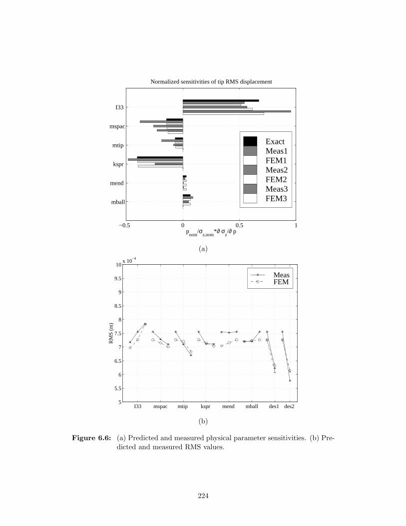
−0.5 0 0.5 1

I33

mspac

mtip

kspr

mend

mball

pnom

/σz,nom

*∂ σz/∂ p

Normalized sensitivities of tip RMS displacement

ExactMeas1FEM1Meas2FEM2Meas3FEM3

(a)

I33 mspac mtip kspr mend mball des1 des2 5

5.5

6

6.5

7

7.5

8

8.5

9

9.5

10x 10

−4

RM

S (

m)

MeasFEM

(b)

Figure 6.6: (a) Predicted and measured physical parameter sensitivities. (b) Pre-dicted and measured RMS values.

224

squared transfer function across the frequency range 10 to 50 Hz.

σz =

[∫ 50 Hz

10 Hz2 |Gzw(f)|2 df

]12

(6.8)

The constraint on the lower frequency limit was due to accelerometer noise. Since the

load cell-to-accelerometer transfer function was integrated twice to obtain Gzw, the low

frequency noise was amplified, and integrating under this portion of the PSD overestimated

the true displacement RMS. Since analysis showed that the contribution to the RMS by

frequencies below 10 Hz was not appreciable, this lower limit was not considered a problem.

The upper limit was set by the maximum frequency available in the measured transfer

function, and it, too, was considered adequate. The RMS measurements for several of the

testbed configurations are presented in Figure 6.6(b). For configurations with multiple data

sets, the RMS values represent an averaged quantity.

Normalized sensitivities from experimental data were determined by using the following

finite-difference approximation.

pnom

(σz)nom

∂σz

∂p≈

σz−(σz)nom(σz)nom

p−pnom

pnom

(6.9)

The gray bars in Figure 6.6(a) represent the values of this approximation corresponding to

each of the modified configurations, except for the two marked with an asterisk, in Table 6.5.

The two configurations not included produced inconsistent results. This is not surprising

since they are associated with the smallest parameter variations in their respective groups.

If the parameter variations are too small, then the anticipated change in the frequency of

the modes can be on the same order as the test-to-test variation in the frequency. In other

words, repeatability issues tend to become more important as the size of the perturbation

becomes smaller. Another point that should be made is that it is not the absolute percent

parameter change that is important, but rather it is the effect that the parameter change

has on the resonant frequencies in the transfer function. Since the performance is related to

the area beneath the squared transfer function, it is critical that the change in the modal

frequencies be captured accurately. If a 10% change in parameter A results in a 1% change

in a dominant frequency, while a 10% change in parameter B results in only a 0.1% change,

then the calculated sensitivity based on A should be a better estimate than the sensitivity

based on B. The parameter variations should be large enough to cause a frequency shift

that is as great as either the frequency resolution or the scatter in repeated tests.

225

This highlights the general difficulty in validating the analytical sensitivities. The pa-

rameter variations need to result in a good signal-to-noise ratio, where the “signal” is the

measured RMS change and the “noise” is the variation in RMS due to non-ideal repeata-

bility. On the other extreme, the parameter variations should be small enough such that

the finite-difference approximation for the sensitivity is still valid. A step that was taken to

minimize the repeatability issue was that multiple nominal transfer functions were taken,

especially when tests were conducted on different days. The RMS value from a test on the

modified system was compared to the nominal RMS value (σz)nom computed from the most

recent nominal transfer function measurement. These two RMS values were then used in

Eq. 6.9. For cases when several data sets existed for a given parameter change, the individ-

ual sensitivities were determined, and then an average was taken. Thus, some of the gray

bars in Figure 6.6(a) are based on this averaging technique.

The white bars in Figure 6.6(a) represent the sensitivities obtained by making the cor-

responding parameter change in the updated FEM, computing the new RMS after perform-

ing a Lyapunov disturbance analysis, and then using the finite-difference approximation

in Eq. 6.9. The RMS predictions for several of the testbed configurations are presented

in Figure 6.6(b), and most come close to the measured RMS values. Each white bar in

Figure 6.6(a) is associated with the gray bar above it. This FEM-based finite-difference

approach served two purposes. First, it helped to validate the analytical sensitivities, and

second, it was used to examine the range of parameter variations for which the linear sensi-

tivity approximation was valid. The only parameter for which this approximation was not

valid is I33. The difference between the exact sensitivity and the FEM approximation is

apparent for all of the shim thickness changes that were tried. The results for all of the

other cases reveal that the sensitivity is rather constant for the magnitude of parameter

modifications that were implemented.

A glance at Figure 6.6(a) indicates that the experimental results capture the same

trends as predicted by the physical parameter sensitivity technique. Although the measured

sensitivities do not exactly match the analytical sensitivities, they have the correct sign,

and they do indicate the order of importance of the parameters (in terms of magnitude

of the sensitivity). Achieving more accurate results in an absolute sense is difficult due to

some of the experimental issues that have already been discussed. One recommendation is to

perform more repeated tests in order to obtain many data sets for each parameter variation.

226

It is anticipated that averaging the results from more trials will reduce the discrepancies

that exist; however, the results from Figure 6.6(a) are quite promising, and it would be a

fair statement to say that the analytical sensitivities have been validated.

The plots in Figures 6.7 and 6.8 are sample PSD and cumulative RMS curves for two

types of parameter variations. Figure 6.7 compares the measured and the predicted curves

for variations in I33, while Figure 6.8 compares the measured and the predicted curves

for variations in kspr. These plots are meant to demonstrate how dependent the overall

RMS value is on the location and height of the resonant peaks. For instance, the fact

that the height of the first peak of the dash-dot measured PSD in Figure 6.7 is slightly

lower than in the predicted dash-dot PSD causes the overall RMS value to be slightly lower

than expected. This results in an overprediction of the sensitivity magnitude. A difference

between the measured and predicted first peak in Figure 6.8 also contributes to errors in

the sensitivity computations. They cause the 4-spring case to underpredict and the 2-spring

case to overpredict the sensitivity magnitude. Although the trends in the PSD curves are

captured well in the data, it is the effect of small differences such as these that make it

challenging to match the measurement-based sensitivities with the analytical sensitivities.

Another issue of practical importance is whether un-updated models can be used to

make redesign decisions based on a physical parameter sensitivity analysis. As a first step

toward answering this, the physical parameter sensitivity code was applied to both types of

un-updated models. The resulting sensitivities are compared to those based on the updated

model, and they are shown in Figure 6.9. With the exception of un-updated model #1’s

estimate of the I33 sensitivity, the un-updated models do a good job of predicting the correct

sign and the relative order of importance of the parameters. It is not surprising that there

are errors in the magnitude of the sensitivities, but the general trend is a good indication. A

conclusion that can be drawn from this one case study is that models that do not have the

benefit of test data, yet do capture the important modes, can still be used to identify critical

structural parameters in the system. Since un-updated model #1 did not predict even the

correct sign of the I33 sensitivity, this points to the need for creating a good first-generation

FEM that uses all available information and past experience.

227

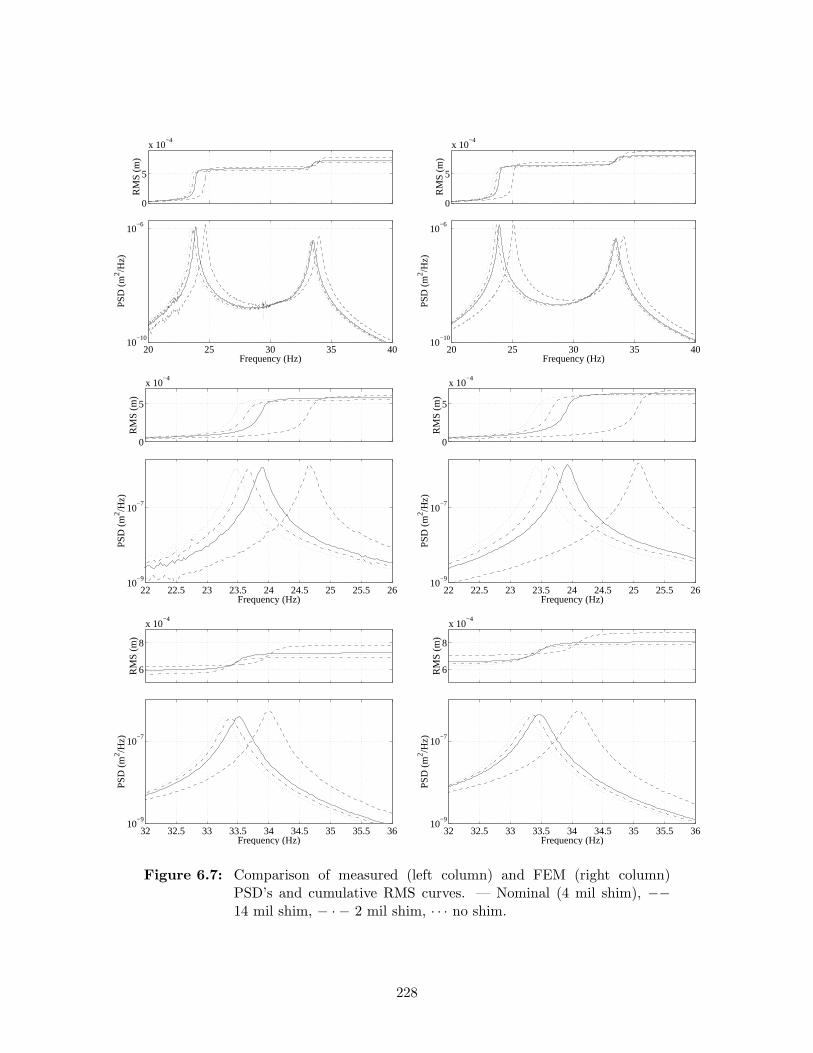
0

5

x 10−4

RM

S (

m)

20 25 30 35 4010

−10

10−6

PS

D (

m2 /Hz)

Frequency (Hz)

0

5

x 10−4

RM

S (

m)

20 25 30 35 4010

−10

10−6

PS

D (

m2 /Hz)

Frequency (Hz)

0

5

x 10−4

RM

S (

m)

22 22.5 23 23.5 24 24.5 25 25.5 2610

−9

10−7

PS

D (

m2 /Hz)

Frequency (Hz)

0

5

x 10−4

RM

S (

m)

22 22.5 23 23.5 24 24.5 25 25.5 2610

−9

10−7

PS

D (

m2 /Hz)

Frequency (Hz)

6

8

x 10−4

RM

S (

m)

32 32.5 33 33.5 34 34.5 35 35.5 3610

−9

10−7

PS

D (

m2 /Hz)

Frequency (Hz)

6

8

x 10−4

RM

S (

m)

32 32.5 33 33.5 34 34.5 35 35.5 3610

−9

10−7

PS

D (

m2 /Hz)

Frequency (Hz)

Figure 6.7: Comparison of measured (left column) and FEM (right column)PSD’s and cumulative RMS curves. — Nominal (4 mil shim), −−14 mil shim, − · − 2 mil shim, · · · no shim.

228

0

5

x 10−4

RM

S (

m)

20 25 30 35 4010

−10

10−6

PS

D (

m2 /Hz)

Frequency (Hz)

0

5

x 10−4

RM

S (

m)

20 25 30 35 4010

−10

10−6

PS

D (

m2 /Hz)

Frequency (Hz)

0

5

x 10−4

RM

S (

m)

23 23.5 24 24.5 2510

−8

10−6

PS

D (

m2 /Hz)

Frequency (Hz)

0

5

x 10−4

RM

S (

m)

23 23.5 24 24.5 2510

−8

10−7

PS

D (

m2 /Hz)

Frequency (Hz)

6

8

x 10−4

RM

S (

m)

32 32.5 33 33.5 34 34.5 3510

−9

10−7

PS

D (

m2 /Hz)

Frequency (Hz)

6

8

x 10−4

RM

S (

m)

32 32.5 33 33.5 34 34.5 3510

−9

10−7

PS

D (

m2 /Hz)

Frequency (Hz)

Figure 6.8: Comparison of measured (left column) and FEM (right column)PSD’s and cumulative RMS curves. — Nominal (0 soft springs), −−2 soft springs, − · − 4 soft springs.

229

−0.6 −0.4 −0.2 0 0.2 0.4 0.6 0.8

I33

mspac

mtip

kspr

mend

mball

pnom

/σz,nom

*∂ σz/∂ p

Normalized sensitivities of tip RMS displacement

Unupdated 1Unupdated 2Updated

Figure 6.9: Predicted physical parameter sensitivities based on different finite-element models.

6.6 Performance Enhancement Exercise

Once the experimental validation of the physical parameter sensitivities had been completed,

the next step was to use the results to suggest redesigns of the testbed that would lead to

a lower RMS tip displacement. Prior to doing this, weighting factors were applied to the

analytical sensitivities so that a fair comparison could be made. Recall that two of the mass

parameters (mspac and mball) govern the mass added at several node locations, while the two

other mass parameters (mtip and mend) affect the mass added at only a single node location.

Dividing the normalized sensitivity by the nominal parameter value and multiplying by the

anticipated largest allowable parameter change results in a quantity that represents the

maximum anticipated percent change in the performance RMS due to the change in the

parameter. This can be seen as follows.

∆pmax

pnom

pnom

(σz)nom

∂σz

∂p× 100% ≈ maximum % change in σz due to change in p (6.10)

As mentioned previously, the physical parameter sensitivity values suggest that the

desired modifications are those that either increase the frequency of the truss or decrease

the frequency of the flexible appendage. The former can be thought of as making the truss

harder to disturb by having the disturbance force push against a stiffer structure. The

230

latter can be thought of as isolating the motion of the appendage tip from the motion of

the end of the truss. The nominal structure was designed based on a priori knowledge

of these redesign options. The nominal shim thickness was nonzero to allow the thickness

to be decreased, thereby lowering the frequency of the appendage. Washers were placed

at all the node locations and hex nuts were placed on the plate to allow mass to be easily

removed from the truss. Soft springs could be added in parallel with the existing stiff spring

to increase the truss mode frequency.

With these options available, the following hypothetical design problem related to the

nominal testbed was posed. What mass and stiffness modifications should be made to

decrease the tip displacement RMS subject to the following constraints?

1. A maximum of four soft springs can be added to the structure.

2. The maximum change in the truss mass is 102 g. (This approximately equals the mass

of the two large hex nuts on the plate. It also represents the total mass of the washers

at all the node locations.)

3. The maximum change in the flexible appendage mass is 2.9 g. (This approximately

equals the mass of two small nuts at each of the 8 spacer locations.)

4. The maximum change in the flexible appendage thickness is 4 mil.

According to Eq. 6.10, a decrease in the performance RMS (i.e., a negative % change)

can be achieved by increasing (decreasing) the value of the parameter if the sensitivity is

negative (positive). Choosing the correct parameter changes and substituting the design

constraints into Eq. 6.10 produced the weighted sensitivities shown in Figure 6.10. The

sensitivity information has been converted into a form that can be directly used to suggest

the design improvements.

The purpose of constraints 2 and 3 was to allow a choice to be made between either

changing the distributed mass or a lumped mass at a key location. For example, constraint 2

leads to the following question. If 102 g can be removed from the truss, is it better to

remove it equally from all portions of the truss or to remove it all from near the tip of

the truss? Constraints 1 and 4 reflect the desire to minimize the stiffness modifications.

Examining Figure 6.10 leads to the conclusion that changing the lumped mass at the tip of

the appendage will lead to the largest performance improvement. Changing the appendage

231

−7 −6 −5 −4 −3 −2 −1 0

mball

mend

kspr

mtip

mspac

I33

% RMS change

Figure 6.10: Weighted sensitivities.

stiffness and the truss spring stiffness are the next most important modifications, followed

by changes in the lumped mass at the plate location and the distributed mass on the

appendage and the truss.

Based on these results, the suggested testbed modifications are:

• Add 2.9 g to the tip of the flexible appendage.

• Reduce the flexible appendage shim thickness from 4 mil to 0mil.

• Add four soft springs.

• Remove the two large nuts from the plate.

This is exactly the case represented by Redesign 1 in Table 6.5. The resulting RMS dropped

from the nominal measured value of 0.755 mm to a value of 0.623 mm (refer to Figure 6.6(b)).

This represents a 17.5% improvement in the tip displacement RMS. The predicted perfor-

mance improvement based on adding the values in Figure 6.10 corresponding to mtip, I33,

kspr, and mend is 16.1%. Thus, the weighted sensitivities proved to be an accurate and

useful design aid.

Redesign 2 in Table 6.5 was used to explore the possibility of obtaining the same or

greater reduction in the tip displacement RMS with less change in the overall mass. Con-

straint 3 was ignored, and 4.2 g was added at the appendage tip without changing the truss

232

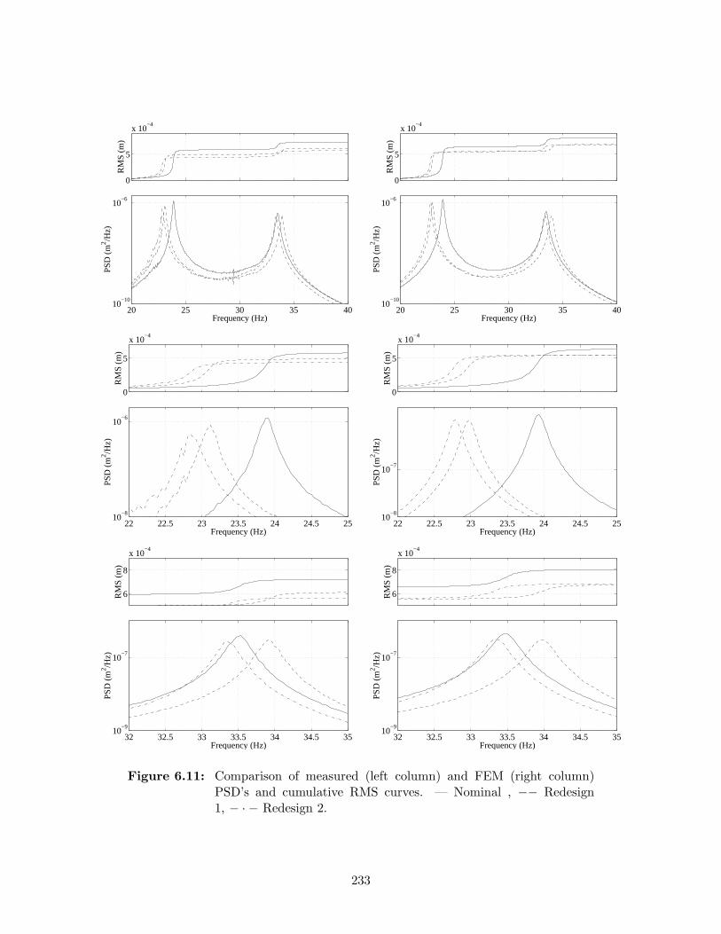
0

5

x 10−4

RM

S (

m)

20 25 30 35 4010

−10

10−6

PS

D (

m2 /Hz)

Frequency (Hz)

0

5

x 10−4

RM

S (

m)

20 25 30 35 4010

−10

10−6

PS

D (

m2 /Hz)

Frequency (Hz)

0

5

x 10−4

RM

S (

m)

22 22.5 23 23.5 24 24.5 2510

−8

10−6

PS

D (

m2 /Hz)

Frequency (Hz)

0

5

x 10−4

RM

S (

m)

22 22.5 23 23.5 24 24.5 2510

−8

10−7

PS

D (

m2 /Hz)

Frequency (Hz)

6

8

x 10−4

RM

S (

m)

32 32.5 33 33.5 34 34.5 3510

−9

10−7

PS

D (

m2 /Hz)

Frequency (Hz)

6

8

x 10−4

RM

S (

m)

32 32.5 33 33.5 34 34.5 3510

−9

10−7

PS

D (

m2 /Hz)

Frequency (Hz)

Figure 6.11: Comparison of measured (left column) and FEM (right column)PSD’s and cumulative RMS curves. — Nominal , −− Redesign1, − · − Redesign 2.

233

mass. The measured RMS was reduced to 0.578 mm, which represents a 23% decrease.

This was larger than expected, and an inspection of the predicted and measured PSD’s

in Figure 6.11 reveals that the peak of the first mode in the data is smaller than in the

FEM-based PSD.

6.7 Summary

A laboratory testbed was designed and constructed with the purpose of validating the

physical parameter sensitivity technique. The testbed consisted of a truss structure with an

attached flexible appendage. The performance metric was chosen to be the displacement of

the tip of the appendage, and this permitted both a global truss mode and a local appendage

mode to contribute to the performance. The disturbance was applied by a shaker near the

root of the truss. An automated finite-element model update routine was developed that

incorporates a constrained optimization algorithm with mode shape and natural frequency

derivatives. The routine converges to physical parameter values that minimize the error

between measured and predicted transfer functions. Mass and stiffness modifications were

made to both the truss and the appendage, and sensitivities derived from experimental

results were compared to the predicted sensitivities from the updated finite-element model.

Although the model-based and measurement-based sensitivities did not match exactly, the

overall trends in both the sign and magnitude level were comparable. Experimental is-

sues that made the measurement of sensitivities challenging were discussed. The use of

un-updated models was also examined, and results indicated that a poor, initial FEM can

actually predict the wrong sign for the sensitivities. A better initial FEM does capture the

overall trends in the sensitivities and can lead to proper redesign choices. An example design

exercise confirmed that a combination of a truss mode frequency increase and a appendage

mode frequency decrease does lead to a smaller tip displacement RMS. It also showed that

changes in tip end mass are more effective than an equivalent change in distributed mass.

Furthermore, the design problem highlighted the fact that design decisions based solely

on modal parameter sensitivity results can lead to unexpected performance changes. Now

that more confidence has been gained related to the use of physical parameter sensitivi-

ties, a performance enhancement technique that utilizes this analysis can be described and

implemented on a model of SIM Classic.

234

Chapter 7

Performance Enhancement

Framework

The disturbance and uncertainty analysis tools can be classified as methods that are used

during the performance assessment of a system. The last major tool that would complete

the overall conceptual design analysis framework pictured in Figure 1.1 is a performance en-

hancement (a.k.a. system improvement) tool. This chapter will describe an initial attempt

at a performance enhancement methodology that utilizes information provided by the pre-

vious analyses. The goal of the initial effort toward this end is not to define a complicated

optimization problem which must be solved, but rather to use all the results to help “point”

in the direction of an improved design and to estimate how “far” to move in that direction.

Trade studies are used first to identify a design that is in the vicinity of the performance

requirements, then minor structural changes are identified that further improve the perfor-

mance. This is where a sensitivity analysis with respect to physical parameters can provide

an important link between the assessment and enhancement portions of the approach. After

the preliminary enhancement methodology is introduced, it will then be implemented on

the model of SIM Classic to demonstrate its use on a complicated, closed-loop system.

7.1 Methodology

As mentioned previously in Chapter 1, much research has been conducted in the area

of simultaneous control-structure optimization. The objective is to choose controller and

structural topologies and/or controller and structural parameters that improve certain per-

235

formance metrics (e.g., mass, control effort, motion errors, etc.) subject to specified system

constraints. Prior to this, work primarily concentrated on optimizing a controller for a given

structural configuration or optimizing the structure for a given controller configuration. Due

to the inherent difficulty in simultaneous optimization, the proposed methodology will focus

on structural redesign options for a given controller.

A fundamental assumption is that a nominal point design exists. This design is based

on a combination of system-level constraints (e.g., total mass, location of optical elements,

packaging restrictions, deployment issues, launch load requirements, etc.) and previous

experience with similar systems (e.g., control design heritage, use of similar structural

components). For high performance systems which rely on closed-loop control to achieve

the requirements, nominal control designs are also assumed to exist.

Figure 7.1 shows the different technologies typically found in controlled structural sys-

tems [15]. They represent a variety of options for modifying the disturbance-to-performance

transmission path. Input isolation attenuates the transmission of disturbance-induced vi-

brations that enter the structure, while output isolation attenuates the transmission of

structural-based vibrations that affect the performance metrics. Passive damping treat-

ments serve to reduce the magnitude of response of system modes that contribute to the

performance. Active structural control loops that use a suite of sensors and actuators fur-

ther modify the system characteristics. Another option, which is implicit in Figure 7.1, is

the relocation/modification of disturbances and/or performances. Examples of this include

restricting reaction wheel speed ranges and moving a disturbance source to a point on a

structure that is a node (zero displacement) of a critical mode.

The general performance enhancement methodology will be described in terms of this

controlled structures technology (CST) framework. Once the performance assessment phase

is completed and it is determined that performance requirements cannot be satisfied or a

sufficient design margin does not exist, then disturbance and/or performance isolation is

implemented first to obtain large performance improvements. Isolation is typically very

effective in achieving orders of magnitude improvement. Along with this, the option for dis-

turbance and performance relocation should be investigated. If a design is obtained whose

predicted performance is close to the desired requirement, then small structural modifica-

tions (based on physical parameter sensitivities) and increased passive damping (based on

modal parameter sensitivities) can be used in tandem to “fine tune” the performance. The

236

InputIsolation Structure Output

Isolation

PassiveDamping

Disturbances Performances

Actuators Sensors

ActiveStructuralControl

?6

- --

?

-

6

-

Redesign

Figure 7.1: Controlled structures technology framework.

performance can be adjusted such that even worst-case predictions from an uncertainty

analysis meet the requirements. If, however, a combination of isolation, damping, and mi-

nor structural redesigns does not prove to be successful, then more ambitious efforts such as

active structural control and major topological redesigns should be pursued. In such a case,

the benefits of combined control-structure optimization will probably be more apparent,

and identifying design options that strive to optimize the control-structure interaction will

be worthwhile. The steps of this methodology are summarized in Table 7.1.

7.2 Application to SIM Classic

This performance enhancement approach will now be demonstrated on the integrated model

of SIM. The first step is to conduct a series of trade studies to identify the changes in

performance that can be accomplished through

• changes in hexapod isolator corner frequency (disturbance isolation),

• application of various levels of optical control (performance isolation), and

• RWA speed restrictions (disturbance modification).

237

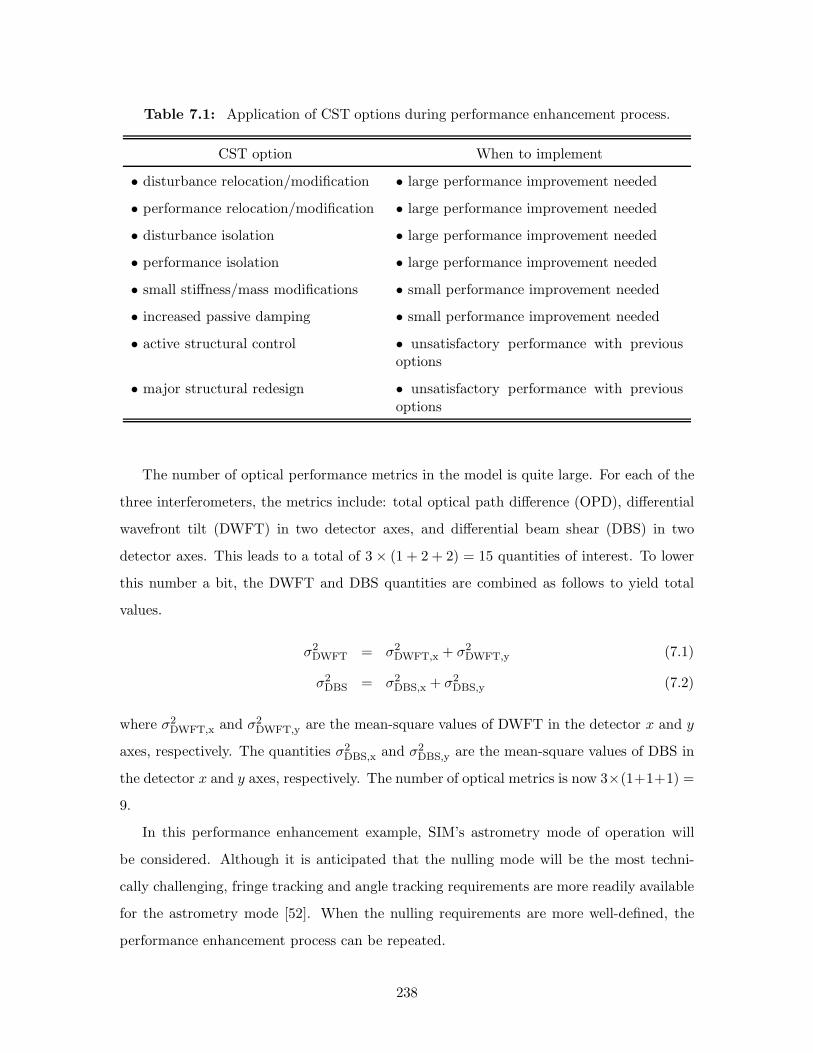
Table 7.1: Application of CST options during performance enhancement process.

CST option When to implement

• disturbance relocation/modification • large performance improvement needed

• performance relocation/modification • large performance improvement needed

• disturbance isolation • large performance improvement needed

• performance isolation • large performance improvement needed

• small stiffness/mass modifications • small performance improvement needed

• increased passive damping • small performance improvement needed

• active structural control • unsatisfactory performance with previousoptions

• major structural redesign • unsatisfactory performance with previousoptions

The number of optical performance metrics in the model is quite large. For each of the

three interferometers, the metrics include: total optical path difference (OPD), differential

wavefront tilt (DWFT) in two detector axes, and differential beam shear (DBS) in two

detector axes. This leads to a total of 3× (1 + 2 + 2) = 15 quantities of interest. To lower

this number a bit, the DWFT and DBS quantities are combined as follows to yield total

values.

σ2DWFT = σ2

DWFT,x + σ2DWFT,y (7.1)

σ2DBS = σ2

DBS,x + σ2DBS,y (7.2)

where σ2DWFT,x and σ2

DWFT,y are the mean-square values of DWFT in the detector x and y

axes, respectively. The quantities σ2DBS,x and σ2

DBS,y are the mean-square values of DBS in

the detector x and y axes, respectively. The number of optical metrics is now 3×(1+1+1) =

9.

In this performance enhancement example, SIM’s astrometry mode of operation will

be considered. Although it is anticipated that the nulling mode will be the most techni-

cally challenging, fringe tracking and angle tracking requirements are more readily available

for the astrometry mode [52]. When the nulling requirements are more well-defined, the

performance enhancement process can be repeated.

238

The requirement on OPD during fringe tracking is 10 nm RMS; however, error budgeting

allocates approximately 4.4 nm to OPD error due to RWA disturbances. (This is based

on extrapolating the error allocation for the nulling mode [52]). The remaining error is

partitioned among sensor noise, actuator resolution, and quantization contributions. The

requirement on angle tracking is 1.6µrad (330 milli-arcsec) RMS, and assuming the same

proportion for error budget allocation leads to a requirement on RWA disturbance-induced

DWFT of 0.704µrad. No specific requirements on DBS have been identified, but visibility

reduction due to beam shear can be determined by the approximate relation [11]

V ≈ 1− σDBS

d(7.3)

where d is the diameter of the beam, and the approximation is valid for σDBS/d < 0.3.

Figure 7.2 shows the nine performance values as a function of both isolator corner

frequency and amount of optical control. The disturbance model is the same as has been

used in previous chapters, namely a low-order filter approximation to disturbance PSD’s of

four HST wheels with random wheel speeds in the range 0–3000 RPM. The circles represent

the results when no optical control is applied. As expected, no significant difference is seen

between the three interferometers. The OPD requirement is not met even when a 2Hz

isolator is used; however, the DWFT requirement is satisfied with a 5 Hz isolator. Isolators

with corner frequencies below 2Hz are not shown since this frequency is approximately the

limit that can be achieved with current passive isolator technology [16]. No requirement

line is shown for the DBS subplots, but for reference, a value of 1µm results in a visibility

reduction of 3.33×10−4, and a value of 10µm results in a visibility reduction of 3.33×10−3.

Closing the delay line and fringe tracker loops produces the series of curves in Figure 7.2

denoted with ×’s. The control designs are equivalent to those presented in Section 2.2.4.

Recall that the guide interferometers have a control bandwidth of 100 Hz to represent an

observation of a bright star, while the science interferometer has a 1 Hz bandwidth to

represent an observation of a dim science target. As a result, the guide interferometers

are able to achieve lower OPD values than the science interferometer due to their greater

disturbance rejection abilities. For the DWFT and DBS metrics, the open optics () and

closed pathlength control (×) curves overlap. This is not surprising since both DWFT and

DBS are related to the pointing errors in the light beams. Only pathlength control is active,

so OPD should be improved while DWFT and DBS remain virtually unchanged. The guide

239

100

101

102

OP

D (

nm)

Guide 1

100

101

102

Guide 2

100

101

102

Science

10−2

10−1

100

DW

FT

(µ r

ad)

10−2

10−1

100

no iso10 Hz 5 Hz 2 Hz

10−1

100

101

DB

S (µ

m)

no iso10 Hz 5 Hz 2 Hz

10−1

100

101

no iso10 Hz 5 Hz 2 Hz

10−1

100

101

10−2

10−1

100

Open loop

Closed ODL,FT

Closed FSM

Figure 7.2: SIM optical performance metrics as a function of isolator corner fre-quency and levels of optical control. Structural damping = 0.1%.(Based on HST RWA 0–3000 RPM disturbance model.)

240

100

101

102

10−15

10−10

10−5

100

Frequency (Hz)

µ ra

d2 /Hz

0

1

2

µ ra

d

PSD and cumulative RMS (total DWFT (guide 1))

no isolation 10 Hz isolator

100

101

102

10−10

10−5

100

105

nm2 /H

z

Frequency (Hz)

0

100

200

nm

PSD and cumulative RMS (Total OPD (guide 1))

open optics closed ODL,FT

(a) (b)

Figure 7.3: (a) Differential wavefront tilt of guide interferometer #1 with openoptics loops and either no isolation or a 10 Hz isolator. (b) Total OPDof guide interferometer #1 with no isolation and either open or closedoptics loops.

interferometers appear to just barely meet the OPD requirement for a 10 Hz isolator, while

the science interferometer needs at least a 5 Hz isolator.

At this point, a few interesting features can be identified and discussed. The first is

that a 10 Hz isolator appears to make the performance slightly worse compared to the no

isolation case for the DWFT and DBS metrics. Plots of the PSD’s and cumulative RMS

curves for the DWFT of guide 1 are presented in Figure 7.3(a). It appears that one of

the modes between 10 Hz and 20 Hz is greatly amplified when the design includes a 10 Hz

isolator. Although the dereverberant backbone of the PSD is lowered at high frequencies

due to the isolation, the amplified mode causes the overall RMS to be slightly larger than

the RMS of the model without isolation.

Another surprising result is that the OPD values of guide 1 and guide 2 become larger

for the no isolation case when the ODL and fringe tracker loops are closed. Figure 7.3(b)

plots the PSD’s and cumulative RMS curves for the total OPD of guide 1. Although the

optics loops reduce the low frequency error, a mode near 100 Hz is amplified enough to

cause the RMS to be larger than when the optics loops are open.

To better assess the DWFT and DBS metrics, fast-steering mirror (FSM) loops can be

closed in the model using a 5th order SISO compensator for each of the 12 FSM input-

to-WFT output loops (3 interferometers × 2 arms/interferometer × 1 FSM/arm × 2

axes/FSM). The FSM axes and detector axes are defined such that a FSM local x (or

241

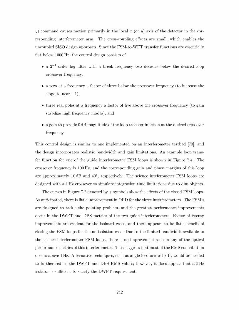
y) command causes motion primarily in the local x (or y) axis of the detector in the cor-

responding interferometer arm. The cross-coupling effects are small, which enables the

uncoupled SISO design approach. Since the FSM-to-WFT transfer functions are essentially

flat below 1000 Hz, the control design consists of

• a 2nd order lag filter with a break frequency two decades below the desired loop

crossover frequency,

• a zero at a frequency a factor of three below the crossover frequency (to increase the

slope to near −1),

• three real poles at a frequency a factor of five above the crossover frequency (to gain

stabilize high frequency modes), and

• a gain to provide 0 dB magnitude of the loop transfer function at the desired crossover

frequency.

This control design is similar to one implemented on an interferometer testbed [70], and

the design incorporates realistic bandwidth and gain limitations. An example loop trans-

fer function for one of the guide interferometer FSM loops is shown in Figure 7.4. The

crossover frequency is 100 Hz, and the corresponding gain and phase margins of this loop

are approximately 10 dB and 40, respectively. The science inteferometer FSM loops are

designed with a 1 Hz crossover to simulate integration time limitations due to dim objects.

The curves in Figure 7.2 denoted by + symbols show the effects of the closed FSM loops.

As anticipated, there is little improvement in OPD for the three interferometers. The FSM’s

are designed to tackle the pointing problem, and the greatest performance improvements

occur in the DWFT and DBS metrics of the two guide interferometers. Factor of twenty

improvements are evident for the isolated cases, and there appears to be little benefit of

closing the FSM loops for the no isolation case. Due to the limited bandwidth available to

the science interferometer FSM loops, there is no improvement seen in any of the optical

performance metrics of this interferometer. This suggests that most of the RMS contribution

occurs above 1Hz. Alternative techniques, such as angle feedforward [61], would be needed

to further reduce the DWFT and DBS RMS values; however, it does appear that a 5Hz

isolator is sufficient to satisfy the DWFT requirement.

242

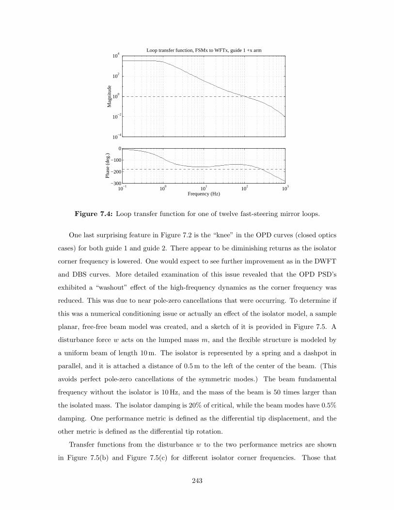
10−4

10−2

100

102

104

Mag

nitu

de

Loop transfer function, FSMx to WFTx, guide 1 +x arm

10−1

100

101

102

103

−300

−200

−100

0

Frequency (Hz)

Pha

se (

deg.

)

Figure 7.4: Loop transfer function for one of twelve fast-steering mirror loops.

One last surprising feature in Figure 7.2 is the “knee” in the OPD curves (closed optics

cases) for both guide 1 and guide 2. There appear to be diminishing returns as the isolator

corner frequency is lowered. One would expect to see further improvement as in the DWFT

and DBS curves. More detailed examination of this issue revealed that the OPD PSD’s

exhibited a “washout” effect of the high-frequency dynamics as the corner frequency was

reduced. This was due to near pole-zero cancellations that were occurring. To determine if

this was a numerical conditioning issue or actually an effect of the isolator model, a sample

planar, free-free beam model was created, and a sketch of it is provided in Figure 7.5. A

disturbance force w acts on the lumped mass m, and the flexible structure is modeled by

a uniform beam of length 10 m. The isolator is represented by a spring and a dashpot in

parallel, and it is attached a distance of 0.5 m to the left of the center of the beam. (This

avoids perfect pole-zero cancellations of the symmetric modes.) The beam fundamental

frequency without the isolator is 10 Hz, and the mass of the beam is 50 times larger than

the isolated mass. The isolator damping is 20% of critical, while the beam modes have 0.5%

damping. One performance metric is defined as the differential tip displacement, and the

other metric is defined as the differential tip rotation.

Transfer functions from the disturbance w to the two performance metrics are shown

in Figure 7.5(b) and Figure 7.5(c) for different isolator corner frequencies. Those that

243

correspond to the differential tip displacement do exhibit pole-zero cancellations as the

corner frequency drops from 20 Hz to 2 Hz. This can be more easily seen by examining the

phase plot. The 2 Hz curve has a 180 phase loss at the isolator mode, but the higher modes

contribute little phase change, as is evident by the extremely small phase deviations about

the −180 line. The larger frequency isolator models exhibit more phase loss due to lightly-

damped beam modes that do not have neighboring lightly-damped zeros. The transfer

functions for the differential tip rotation, on the other hand, do not show any signs of the

washout effect. For the different isolator models, they all show large resonant behavior

at the higher frequencies. These results suggest the washout phenomenon is probably

not a numerical conditioning issue, especially due the fact that this example problem is

not extremely complex. In fact, the results are analogous to the trends seen in the SIM

trade studies. The OPD is affected by the loss of observability and/or disturbability of

the higher modes, thereby causing a knee in the curves. DWFT and DBS do benefit

from the additional isolation since the highly-resonant modes at higher frequencies which

normally would contribute to the performance are being lowered in magnitude due to the

isolation. Further work is recommended in order to confirm these findings. It should be

noted, however, that the results to follow do not heavily depend on the shape of the OPD

curves for lower corner frequency isolators.

Thus far, both performance and disturbance isolation have been examined. The other

CST option that is listed in Table 7.1 and that can be implemented on the SIM model is

disturbance modification. This is one of the options which can achieve large performance

improvement on a nominal design when done properly. The original RWA disturbance model

that was used to obtain the previous results is based on an assumption of wheel speeds in

the 0–3000 RPM range. Now consider the case when the wheel speeds are restricted to

lie within the 0–600 RPM range. It is not known how practical it would be to have a

lower maximum allowable reaction wheel speed during an observation. This might not be

possible during long integration times of extremely dim objects; however, this issue will be

overlooked for now. Plots of the approximate disturbance PSD’s for both the 0-3000 RPM

case and 0–600 RPM case are visible in Figure 7.6. Reducing the maximum wheel speed

serves to reduce significantly the energy at high frequencies; however, this also allows the

wheels to spend more time at the lower speeds. The result is that at low frequencies, the

PSD’s for the 0–600 RPM case actually exceed the PSD’s for the 0–3000 RPM case.

244

x1 x2

θ2

F

isolator

θ1

m

(a)

10−1

100

101

102

103

−1000

−500

0

Frequency (Hz)

Pha

se (

deg.

)

10−12

10−10

10−8

10−6

10−4

(x1−x

2)/F

Mag

nitu

de (

m/N

)

2 Hz iso 5 Hz iso 10 Hz iso20 Hz iso

10−15

10−10

10−5

(θ1−θ

2)/F

Mag

nitu

de (

rad/

N)

10−1

100

101

102

103

−2000

−1000

0

Frequency (Hz)

Pha

se (

deg.

)

(b) (c)

Figure 7.5: (a) Sample system to demonstrate washout effect. (b) Transfer func-tion from disturbance to differential tip displacement for various isola-tors. (b) Transfer function from disturbance to differential tip rotationfor various isolators.

245

100

101

102

103

10−10

10−8

10−6

10−4

Frequency (Hz)

Mag

nitu

de (

N2 /Hz

or (

N−

m)2 /H

z)

Figure 7.6: Disturbance PSD’s for the 0–3000 RPM case (—) and for the 0–600 RPM case (−−).

Rerunning all of the disturbance analyses for various combinations of isolator corner

frequencies and amount of optical control produces the results in Figure 7.7. When the

RMS values are compared to those in Figure 7.2, some distinguishing features become

apparent. First, the only consistent performance improvement in all three metrics occurs

when no isolation is present. This makes sense because without isolation to attenuate

the vibrations that excite the higher frequency modes, the larger energy content of the

0–3000 RPM disturbance at high frequencies (> 20 Hz) passes through easily. As seen

previously in Figure 7.3, modes up to and slightly beyond 100 Hz contribute a noticeable

amount to the RMS values when the model does not have the benefit of isolation. When

isolation is present, it is the lower frequency modes that can contribute the most to the

overall RMS. If these critical modes occur below approximately 17 Hz, then the extra energy

in the 0–600 RPM case at these frequencies can actually make the RMS worse. This could

possibly explain the increase seen in the OPD metrics for the three interferometers when

disturbance isolation is used and optics loops are open.

Another feature is that for the isolated cases of DWFT and DBS, there do not appear

to be significant differences with the corresponding RMS values in the 0–3000 RPM case.

Restricting the wheel speed range does not offer much benefit for these metrics. The PSD’s

and cumulative RMS curves in Figure 7.8(a) provide a clue as to why this is the case.

This plot compares the results of the guide 1 DWFT with all optics loops closed and a

246

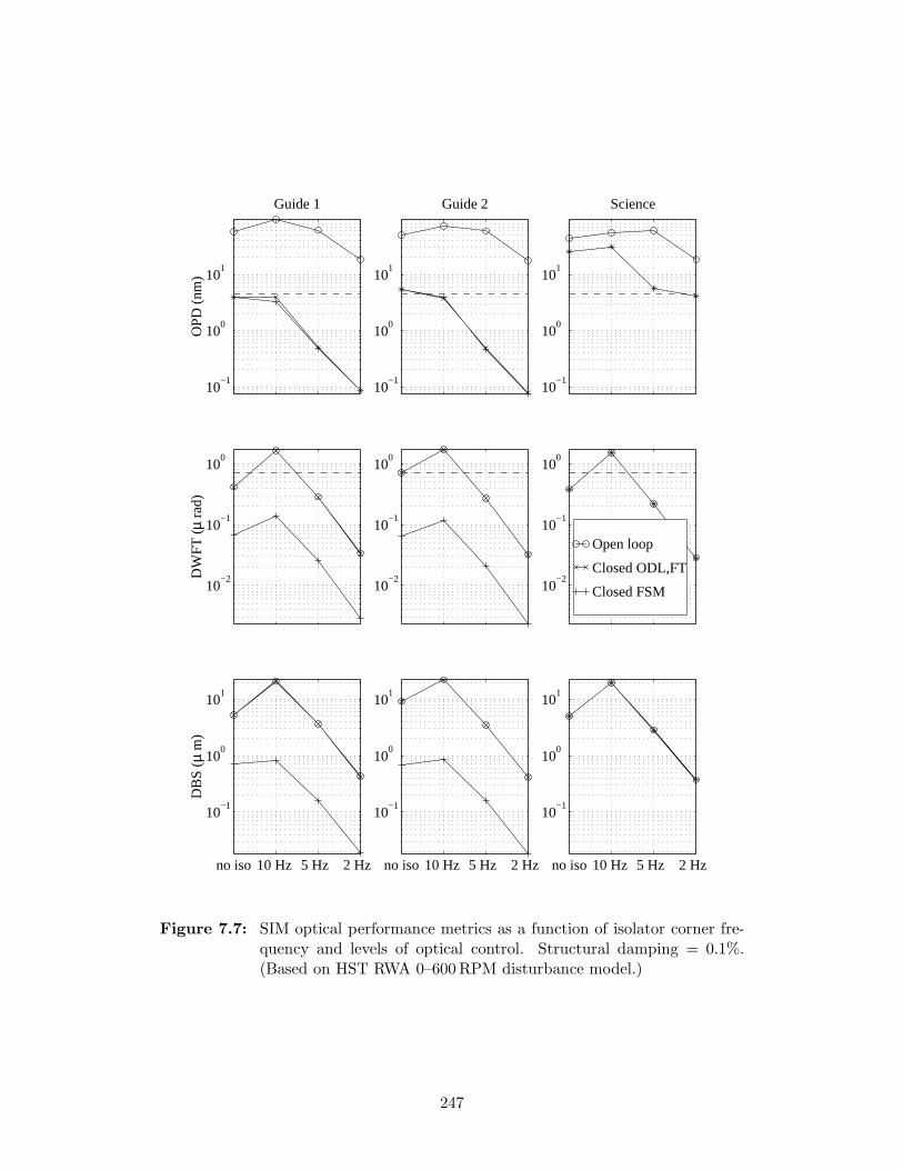
10−1

100

101

OP

D (

nm)

Guide 1

10−1

100

101

Guide 2

10−1

100

101

Science

10−2

10−1

100

DW

FT

(µ r

ad)

10−2

10−1

100

no iso10 Hz 5 Hz 2 Hz

10−1

100

101

DB

S (µ

m)

no iso10 Hz 5 Hz 2 Hz

10−1

100

101

no iso10 Hz 5 Hz 2 Hz

10−1

100

101

10−2

10−1

100

Open loop

Closed ODL,FT

Closed FSM

Figure 7.7: SIM optical performance metrics as a function of isolator corner fre-quency and levels of optical control. Structural damping = 0.1%.(Based on HST RWA 0–600 RPM disturbance model.)

247

100

101

102

103

0

0.1

0.2PSD and cumulative RMS (DWFT (guide 1))

µrad

100

101

102

103

10−20

10−15

10−10

10−5

100

Frequency (Hz)

µrad

2 /Hz

0−3000 RPM 0−600 RPM

100

101

102

103

0

0.5

1

1.5PSD and cumulative RMS (total OPD (guide 1))

nm

100

101

102

103

10−15

10−10

10−5

100

Frequency (Hz)

nm2 /H

z

0−3000 RPM 0−600 RPM

(a) (b)

Figure 7.8: (a) Differential wavefront tilt of guide interferometer #1 with closedFSM loops and either a 0–3000 RPM RWA speed range or a 0-600 RPM speed range (10 Hz isolator). (b) Total OPD of guide inter-ferometer #1 with closed pathlength loops and either a 0–3000 RPMRWA speed range or a 0-600 RPM speed range (5 Hz isolator).

10 Hz isolator. For both wheel speed ranges, the critical mode is near 17 Hz, which is the

frequency around which the disturbance PSD’s in Figure 7.6 have approximately the same

magnitude. Therefore, the lower energy content at higher frequencies for the 0–600 RPM

case does not matter.

The OPD values, however, are affected by the lower wheel speeds. The RMS values

decrease when the optics loops are closed and increase slightly when the optics loops are

open. Figure 7.8(b) compares the PSD’s and cumulative RMS curves of the total OPD

of guide 1 when only the pathlength control loops are closed and there is a 5 Hz isolator.

For the 0–3000 RPM case, the OPD RMS value is dependent on frequencies up to around

200 Hz. When disturbance energy is lowered between 20 Hz and 200 Hz due to restricted

wheel speeds, the resulting RMS is lowered as well (by a factor of about 2 in this example

plot).

Based on all of the results shown so far, the recommended design consists of a 10 Hz

isolator with closed pathlength (ODL, fringe tracker) and pointing (FSM) loops. The re-

action wheel speeds are permitted to take on values over their entire operating regime of

0–3000 RPM. For this level of isolation and optical control, restricting the wheel speeds does

not lead to a performance improvement large enough to justify placing a constraint on the

248

Table 7.2: Comparison of RMS values for different SIM designs.

Optical metric Reqmt. Design 1 Design 2

RMS design margin RMS design margin

Total OPD (g1) 4.4 nm 4.36 nm 0.073 dB 2.71 nm 4.20 dB

Total OPD (g2) 4.4 nm 3.21 nm 2.75 dB 3.53 nm 1.91 dB√J 1.41 1.23 1.21 dB 1.01 2.92 dB

DWFT (g1) 0.704 µrad 0.154 µrad 13.2 dB 0.124 µrad 15.1 dB

DWFT (g2) 0.704 µrad 0.124 µrad 15.1 dB 0.106 µrad 16.5 dB

DBS (g1) N/A 0.996 µm – 0.784 µm –

DBS (g2) N/A 0.949 µm – 0.789 µm –

time between momentum dumps of the wheels. The RMS values of this design (labeled De-

sign 1) are compared to the requirements in Table 7.2. Values for the science interferometer

are intentionally omitted since it is anticipated that other control strategies not currently

in the model will be used to improve the fringe tracking and pointing peformance of this

interferometer. The structural redesigns will focus on improving the performance of the

guide interferometers.

The total OPD metrics have the smallest design margins (0.073 dB and 2.75 dB, re-

spectively). Since the first margin will almost assuredly be used up when a worst-case

uncertainty analysis is conducted, there is a motivation to try to increase the margins a bit.

Based on the performance enhancement methodology in Table 7.1, the next options that

can be implemented are increased passive damping and minor stiffness/mass modifications.

Figure 7.9 shows the RMS values of the optical performance metrics for the 0-3000 RPM

case when the structural damping is increased to 1%. As expected, all of the RMS values are

lower than the results for the models characterized by 0.1% damping. In fact, the DWFT

requirement is satisfied regardless of the presence of isolation or closed optics loops.

To better identify physical parameters that affect the total OPD values for both guide

interferometers, define a weighted cost J as follows.

J =1

σ2OPD,req

(σ2

OPD,g1 + σ2OPD,g2

)(7.4)

249

100

101

OP

D (

nm)

Guide 1

100

101

Guide 2

100

101

Science

10−2

10−1

DW

FT

(µ r

ad)

10−2

10−1

no iso10 Hz 5 Hz 2 Hz 10

−2

10−1

100

DB

S (µ

m)

no iso10 Hz 5 Hz 2 Hz 10

−2

10−1

100

no iso10 Hz 5 Hz 2 Hz 10

−2

10−1

100

10−2

10−1

Open loop

Closed ODL,FT

Closed FSM

Figure 7.9: SIM optical performance metrics as a function of isolator corner fre-quency and levels of optical control. Structural damping = 1%.(Based on HST RWA 0–3000 RPM disturbance model.)

250

Since the OPD of guide 1 is the metric with the smallest margin, there might be a temptation

to carry only this metric into a disturbance and sensitivity analysis to identify important

structural parameters. However, a structural modification that improves σOPD,g1 is not

guaranteed to improve σOPD,g2. The combined cost J allows identification of structural

enhancements that attempt to improve both metrics. The DWFT metrics, on the other

hand, have sufficient design margin and do not need to be included in the cost function.

Only small structural modifications will be implemented, and they should not drastically

reduce the design margins of the DWFT metrics. (The design margins will be checked,

however, after the redesign is implemented.)

A frequency-domain disturbance analysis produces the cumulative RMS curve, PSD, and

disturbance contribution plot in Figure 7.10(a). The bar char in Figure 7.10(b) summarizes

these results, and it is apparent that the mode at 16.95 Hz contributes about 25% of the

total value of J . Other critical modes are at 12.3 Hz and 18.91 Hz. Several of the modes

listed are almost entirely excited by the reaction wheel Mz disturbance. The sensitivities

of the square-root of J with respect to modal parameters are plotted in Figure 7.10(c), and

the critical modes identified from this plot do correspond to those in Figure 7.10(b), as

expected. Assuming ±5% uncertainty in the frequencies of the three most critical modes,

a first-order uncertainty analysis predicts an approximately 7% increase in the square-root

of J (14% increase in J).

Mode shape and strain energy distribution plots for the modes at 16.95 Hz, 18.91 Hz,

and 21.39 Hz were shown in Section 4.6.2. Recall that the first mode is characterized by

siderostat boom torsion and the latter two modes are characterized by local siderostat bay

modes. The 12.3 Hz mode is one of the six hexapod modes. Three parameters were chosen

for the physical parameter sensitivity analysis. They are the torsional constant J of the

siderostat boom cross section (not to be confused with the cost J), a stiffness scale factor

α used to adjust all of the siderostat bay stiffnesses simultaneously, and a mass scale factor

β used to adjust all of the siderostat bay masses simultaneously. The sensitivities of the

square-root of J with respect to these parameters are shown in Figure 7.11. Assuming that

a 1% change in each of these parameters “costs” approximately the same to implement, then

the torsional constant J provides the largest performance improvement potential, followed

by the siderostat bay parameters α and β. All three sensitivities are positive, which indicates

that performance improvement (i.e., cost reduction) is achieved by decreasing the values of

251

0

1

2

unit

PSD and cumulative RMS (J (weighted outputs))

10−10

10−8

10−6

10−4

10−2

100

102

unit2 /H

z

100

101

102

FxFyFz

MxMyMz

Disturbance Contribution

Frequency (Hz)

Dis

turb

ance

(a)

12.30 16.95 18.91 20.86 21.39 46.23 61.40 96.690

5

10

15

20

25

30

Critical frequencies (Hz)

% c

ontr

ibut

ion

J (weighted outputs)

RWA Fx RWA Fy RWA Fz RWA Mx RWA My RWA Mz

−0.3 −0.2 −0.1 0 0.1 0.2 0.3 0.4 0.5 0.6

12.3

16.95

18.09

18.91

20.86

21.39

22.17

46.24

61.4

96.69

Normalized Sensitivities of J (weighted outputs)

Ope

n−lo

op m

odal

freq

uenc

y (H

z)

pnom

/σz,nom

*∂ σz /∂ p

p = ωp = ζ p = m

(b) (c)

Figure 7.10: (a) PSD, cumulative RMS, and disturbance contribution plots ofweighted OPD for guide 1 and guide 2. (b) Critical modes anddisturbances. (b) Modal parameter sensitivities of weighted OPD.

252

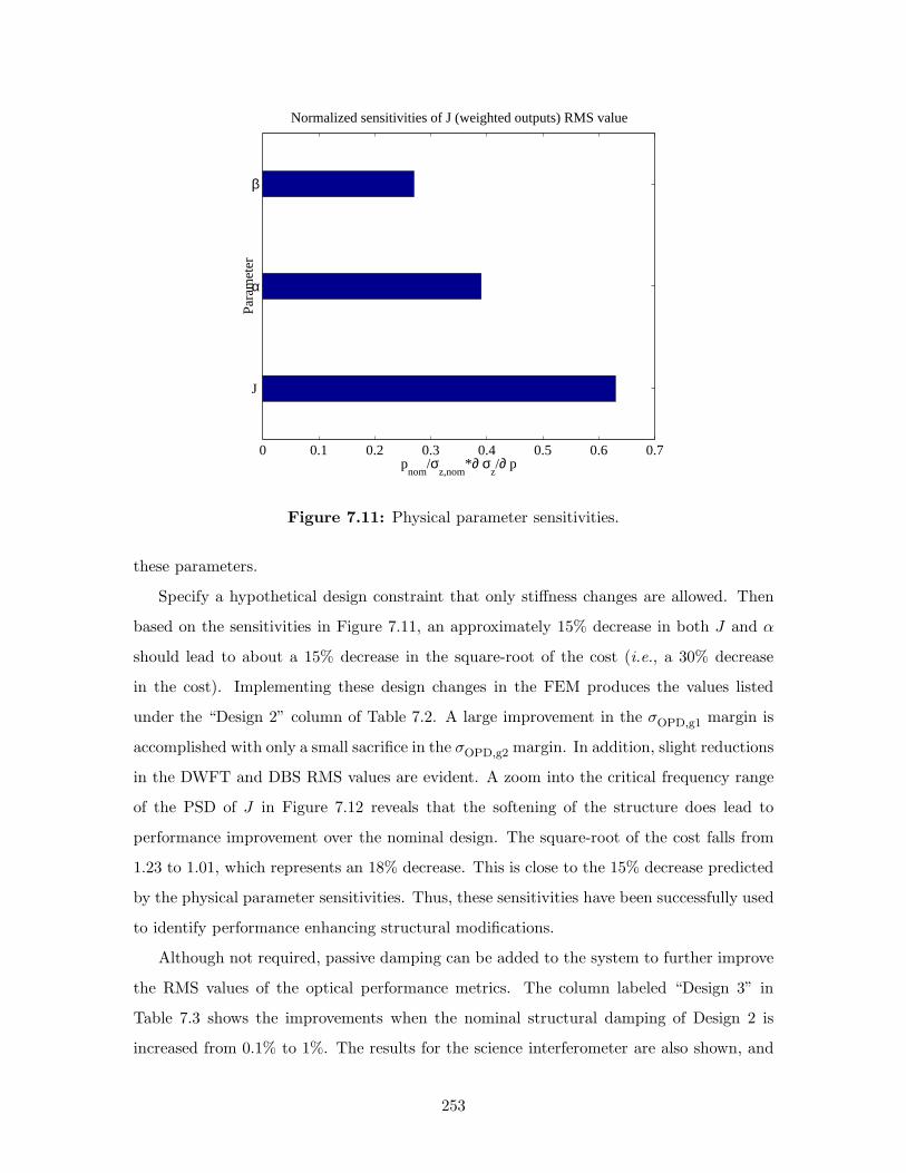
0 0.1 0.2 0.3 0.4 0.5 0.6 0.7

Normalized sensitivities of J (weighted outputs) RMS value

pnom

/σz,nom

*∂ σz/∂ p

Par

amet

er

α

J

β

Figure 7.11: Physical parameter sensitivities.

these parameters.

Specify a hypothetical design constraint that only stiffness changes are allowed. Then

based on the sensitivities in Figure 7.11, an approximately 15% decrease in both J and α

should lead to about a 15% decrease in the square-root of the cost (i.e., a 30% decrease

in the cost). Implementing these design changes in the FEM produces the values listed

under the “Design 2” column of Table 7.2. A large improvement in the σOPD,g1 margin is

accomplished with only a small sacrifice in the σOPD,g2 margin. In addition, slight reductions

in the DWFT and DBS RMS values are evident. A zoom into the critical frequency range

of the PSD of J in Figure 7.12 reveals that the softening of the structure does lead to

performance improvement over the nominal design. The square-root of the cost falls from

1.23 to 1.01, which represents an 18% decrease. This is close to the 15% decrease predicted

by the physical parameter sensitivities. Thus, these sensitivities have been successfully used

to identify performance enhancing structural modifications.

Although not required, passive damping can be added to the system to further improve

the RMS values of the optical performance metrics. The column labeled “Design 3” in

Table 7.3 shows the improvements when the nominal structural damping of Design 2 is

increased from 0.1% to 1%. The results for the science interferometer are also shown, and

253

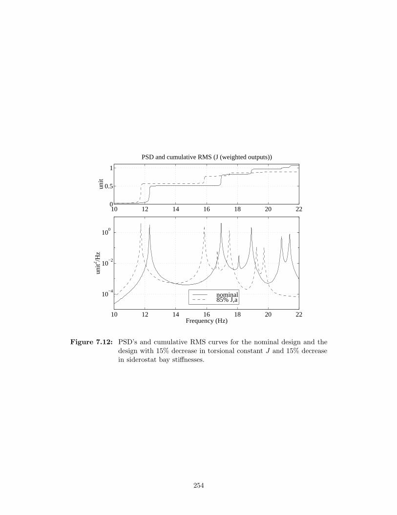
10 12 14 16 18 20 220

0.5

1

PSD and cumulative RMS (J (weighted outputs))

unit

10 12 14 16 18 20 22

10−4

10−2

100

Frequency (Hz)

unit2 /H

z

nominal85% J,a

Figure 7.12: PSD’s and cumulative RMS curves for the nominal design and thedesign with 15% decrease in torsional constant J and 15% decreasein siderostat bay stiffnesses.

254

Table 7.3: Comparison of RMS values for different SIM designs.

Optical metric Reqmt. Design 3 Design 4

RMS design margin RMS design margin

Total OPD (g1) 4.4 nm 1.28 nm 10.7 dB 0.907 nm 13.7 dB

Total OPD (g2) 4.4 nm 1.45 nm 9.66 dB 0.939 nm 13.4 dB

Total OPD (s) 4.4 nm 7.27 nm −4.36 dB 1.67 nm 8.4 dB

DWFT (g1) 0.704 µrad 0.044 µrad 24.1 dB 0.0115 µrad 35.8 dB

DWFT (g2) 0.704 µrad 0.0352 µrad 26.0 dB 0.0093 µrad 37.6 dB

DWFT (s) 0.704 µrad 0.446 µrad 3.97 dB 0.0097 µrad 37.2 dB

DBS (g1) N/A 0.344 µm – 0.144 µm –

DBS (g2) N/A 0.277 µm – 0.121 µm –

DBS (s) N/A 5.83 µm – 0.127 µm –

we notice that the requirements are still not being met. The DWFT metrics of the guide

interferometers, though, have no trouble meeting the requirement.

Now consider an ambitious and somewhat radical design consisting of a 2Hz isolator,

1% structural damping, closed pathlength loops, and open FSM loops. The resulting RMS

values are found under the “Design 4” column in Table 7.3. In this case, all three inter-

ferometers have positive design margins for the OPD and DWFT metrics. This design is

unique in that an extremely soft isolator is used to compensate for the limited disturbance

rejection properties of the science pathlength loop. It also allows most of the DWFT errors

to be reduced without the use of FSM control.

Looking ahead to redoing this process for the nulling mode of operation, we can an-

ticipate that the OPD and DWFT requirements will become more stringent by roughly a

factor of 10. If this is this case, then Design 4 will not satisfy the OPD requirements, but

it should still be able to satisfy the DWFT requirements. To accurately assess this mode,

the integrated model will need to incorporate pathlength feedforward techniques (e.g., ac-

celerometer feedforward). In addition, the observation of even fainter science stars than

have been implicitly assumed by the science pathlength and pointing control bandwidths

will also require the use of these feedforward techniques.

255

7.3 Summary

A methodology has been described for improving the performance of a nominal system by

using traditional CST options. Trade studies are conducted first to focus on the disturbance

and performance aspects of the system. When a design is found that satisfies or nearly sat-

isfies requirements, then minor structural changes such as mass and stiffness modifications

or passive damping augmentation are identified that achieve desired design margins. Phys-

ical parameter and modal parameter sensitivity analyses can be conducted to help pinpoint

which changes are the most beneficial. Active structural control or major topological re-

designs are additional options when the other options fail to produce satisfactory results.

The overall performance assessment and enhancement framework was applied to a model

of SIM Classic. Requirements for the astrometry mode of operation were identified, and

trade studies investigated the performance improvements that can be achieved with RWA

isolation, RWA speed restrictions, pathlength control, pointing control, and passive damp-

ing. Focus was placed on improving the performance of the guide interferometers since

feedforward techniques have not yet been implemented to assess the science interferometer.

Results indicate that the pathlength requirements are more difficult to meet, but can be

satisifed through a combination of reaction wheel isolation and pathlength control. The

wavefront tilt metrics, however, can satisfy the pointing requirement with isolation alone

and do not necessarily need to rely on closed FSM loops. Restricting the maximum reaction

wheel speed to be 600 RPM instead of the nominal 3000 RPM did not improve all of the

optical RMS values. The only appreciable benefits were observed in the OPD metrics for

the cases that used isolators with 5 Hz or lower corner frequencies.

Structural modifications based on physical parameter sensitivities were successfully im-

plemented and achieved the predicted amount of design margin increase. The modifications

consisted of decreasing by 15% the torsional rigidity of the siderostat booms and the stiff-

ness of each siderostat bay relative to the siderostat boom. This suggests that further

improvements might be achieved by “tuning” the siderostat bays individually. Additional

RMS reduction was achieved by increasing the damping of the critical modes from 0.1% to

1%.

Although the goal of the design exercise was to improve the system performance during

the astrometry mode, consideration was given to the eventual goal of meeting the nulling

256

requirements. For the 0-3000 RPM RWA case, a design consisting of a 2Hz isolator, closed

pathlength loops, and 1% structural damping failed to meet the OPD requirements; how-

ever, indications are that the DWFT requirements can be achieved. This highlights the

need for pathlength feedforward techniques. The results also suggest that the DWFT error

budget can be revisited such that the allocation to RWA-induced disturbances is lowered

and distributed elsewhere. For instance, noisier yet less costly pointing control sensors

might be permitted.

257

258

Chapter 8

Conclusions and Recommendations

This concluding chapter summarizes the performance assessment and enhancement

framework that has been developed and demonstrated in the preceding chapters. The

major contributions that were made during the course of the development are listed, and

further work that would extend the capabilities of this framework are suggested.

8.1 Thesis Summary

The next generation of space-based scientific observatories are characterized by stringent

tolerances on optical performance metrics. The success of these spacecraft depends greatly

on the ability of optical control and vibration mitigation techniques to provide stabiliza-

tion of collected starlight despite the excitation of flexible structural modes by disturbance

sources. Early design trades and decisions rely on initial analyses that use simplified models

of these high performance systems. A methodology was created that applies a systematic

process to predict the effects of disturbances on the system and to estimate variations

in the predictions due to model uncertainties. In addition, it suggests standard control-

structure-interaction technologies and structural modifications to improve the performance

when needed.

Chapter 2 described the integrated modeling process used to generate models of initial

concepts. Structural dynamic modeling provides the governing equations of motion for

the system and predicts the effect of control and disturbance inputs on the structural

displacements. Optical modeling uses linear ray trace theory to relate the displacements of

optical elements to perturbations in optical metrics such as pathlength and wavefront tilt.

259

Control modeling introduces a compensator that uses outputs of the model to determine

the appropriate control inputs to apply to the system for purposes such as disturbance

rejection or command-following. Disturbance modeling quantifies the magnitude, spectral

content, and location of anticipated disturbances. Chapter 2 reviewed stochastic process

theory and its potential use as a tool for characterizing disturbances. Stochastic process

theory avoids a costly Monte Carlo analysis by producing “expected” disturbance levels;

however, worst-case situations cannot be directly identified. The importance of disturbance

modeling was emphasized, and serious efforts should be placed in this area.

The interplay between the different disciplines suggests that the modeling cannot occur

independently. For instance, structural modeling must provide the locations at which optical

elements exist and disturbance and control forces are applied. Everyone associated with the

integrated modeling process must be aware of the requirements placed by each discipline

on the others. A recommendation related to control modeling during the early conceptual

design process is that the control designs implemented should be realistic, especially in

terms of gain and bandwidth limitations. Performance predictions based on controllers that

assume perfect sensors and actuators and utilize precise knowledge of the plant model will be

misleading. For instance, large predicted performance improvement due to the control might

result in fewer vibration mitigation techniques being incorporated in the design. It might be

difficult to add these technologies to the system after it has been constructed and found to

require them. A consideration of numerical conditioning issues revealed that compensator

state-space representations that are derived from typical numerator-denominator transfer

function form should be transformed into a balanced realization. Furthermore, if model

reduction is to be performed, the model inputs and outputs should be scaled such that the

transfer functions are of similar order of magnitude. This allows modes that are important

in some input/output channels but not others to be retained in the model.

The integrated model of one concept for the Space Interferometry Mission (SIM) was

also described in Chapter 2. This model was developed at the Jet Propulsion Laboratory

and served as a typical spacecraft model on which to demonstrate the analysis tools that

were developed. A new method for generating reaction wheel assembly (RWA) stochastic

disturbance models was introduced. This method extends a current technique that mod-

els only a single wheel explicitly. This approach was used to create Hubble-based RWA

disturbance models that are applied to the SIM model.

260

Chapter 3 reviewed three types of disturbance analyses that can be conducted when a

system is represented in state-space form. A standard time simulation involves numerical

integration of the equations of motion. The integration step size should be small enough

to capture the highest frequencies of interest, but should be large enough such that the

computational time does not become excessive. A simple spring-mass system driven by

white noise showed the fundamental trade between time-simulation length and the accuracy

of the predicted steady-state RMS value.

The second type of disturbance analysis is based on propagating disturbance power

spectral density (PSD) functions through the system transfer functions to obtain the per-

formance PSD’s. The spring-mass system was used to demonstrate the effects of frequency

resolution on the predicted RMS values. More frequency points lead to more accurate es-

timates, but at the cost of increased computation time. The frequency resolution around

lightly-damped modes is particularly critical, and the appropriate resolution can be deter-

mined by plotting a cumulative RMS curve, which indicates the contribution to the overall

RMS value as a function of frequency. Lightly-damped modes manifest themselves as sharp

“steps” in the cumulative RMS function, and accurate RMS estimates require that a suffi-

cient number of frequency points define each step. The cumulative RMS function can also

be used to determine if the number of modes retained in the model is sufficient. A cumu-

lative RMS curve that is still rising after the last mode has been reached is an indication

that additional modes will probably add to the predicted RMS.

A frequency-domain disturbance analysis was also shown to provide information related

to the disturbance contribution at each frequency based on an uncorrelated assumption for

the disturbances. The results of the analysis can be conveniently displayed in bar chart

form. For each mode, the length of the bar is proportional to that mode’s contribution to

the performance variance, and the bar is subdivided according to the relative contribution

from each disturbance. Examining this type of plot quickly conveys the critical modes and

disturbances that affect the performance metrics. A frequency-domain analysis was demon-

strated on the SIM model, and the most critical mode for an optical path difference (OPD)

metric was identified as a boom torsion mode that was excited most by RWA disturbances

about the global z axis. In this example, neglecting the off-diagonal terms in the distur-

bance cross-spectral density matrix was shown to allow quicker computation times without

significant loss in accuracy.

261

The third type of disturbance analysis assumes that the overall state-space system (with

appended disturbance filter dynamics) is excited by pure white noise. A Lyapunov equation

is solved to obtain the state covariance matrix, which can then be transformed to obtain

the performance covariance matrix. This approach produces the exact, theoretical mean-

square values of the various performance metrics. The computation time can be excessive

for large-order models; however, model reduction strategies can produce a smaller system

that retains accurate performance prediction capability.

Using a Lagrange multiplier approach, Chapter 4 derived the exact expression for the

sensitivity (i.e., derivative) of performance RMS values with respect to a generic parameter.

The sensitivities require the solution of one Lyapunov equation for the state covariance ma-

trix plus one Lyapunov equation for the Lagrange multiplier matrix for every performance

metric. Also required are the derivatives of the state-space matrices with respect to the

parameter. A review was provided of the steps to place a structural model in modal, state-

space form. After closing control loops (if present) and placing a disturbance shaping filter

in series with the system, the sensitivity equation can be simplified when the parameter

of interest is a modal frequency, modal mass, or damping ratio of the open-loop structural

system. A normalized sensitivity value can be computed that provides an indication of the

percent change in the RMS values for a percent change in each parameter individually. The

modes with the largest normalized modal parameter sensitivities were shown to correspond

to the critical modes identified from a frequency-domain analysis. The exact sensitivity ap-

proach is more computationally efficient than a finite-difference approach when the number

of parameters of interest exceeds the number of performance variables. Results on the SIM

model indicated that the sensitivities from a finite-difference approach were not numerically

stable as the parameter perturbation size was decreased.

Chapter 4 also described a method for computing sensitivities of performance RMS

values with respect to physical parameters of the structural finite-element model. These

sensitivities provide more intuition from a structural redesign perspective. The method

requires that the derivatives of mode shapes, natural frequencies, and modal masses be

computed with respect to the parameters of interest. An existing code was modified to

include the modal mass derivatives and to accommodate desired parameters such as elastic

spring element constants and lumped mass/inertia values. Necessary modifications were

also made to the equations when the finite-element model consists of independent and

262

dependent degrees of freedom. The physical properties of elements with strong influence on

the critical modes are chosen for the sensitivity analysis, and strain energy distribution plots

help to make this selection. The sensitivity calculations can be computationally intensive

for large models; however, simplifications were identified to reduce the computational effort

with minimal impact on the results. For instance, the method only requires knowledge of

mode shapes at DOF’s associated with inputs and outputs. Also, only those modes that

significantly contribute to the performance need to be retained in the computations. This

was demonstrated on a simple, cantilever beam example problem. Application to the closed-

loop SIM model revealed that the sensitivities of an OPD metric are large with respect to the

torsional rigidity constants G and J of the siderostat booms and the generalized stiffness and

mass properties of a siderostat bay. This appears to be the first attempt in the literature of

computing accurately the performance sensitivities of a large-order (307 states), closed-loop

model with respect to physical parameters.

The effect of model uncertainties on performance RMS predictions was the topic of Chap-

ter 5. A technique was developed that searches for allowable values of modal frequency,

modal mass, and modal damping ratios of specified modes that maximize the predicted

cost. The cost is a weighted combination of performance mean-square values; therefore,

the technique identifies the worst-case performances. The modes with the largest modal

parameter sensitivities are selected for the uncertainty analysis. A constrained optimization

approach is used to identify the worst-case parameters, and multiple runs with different ini-

tial guesses are required to improve confidence that the solution is converging to the global

maximum. In addition, analytical gradient information based on modal parameter sensi-

tivities is supplied to the optimization routine to help the solution process. The result of

applying the technique to a low-order, open-loop system suggests that the worst-case modal

parameters can be identified a priori by placing the parameters at the bounds indicated

by the directional information of the modal parameter sensitivities. A counter-example

was also analyzed that showed the worst-case parameters do not necessarily occur at these

bounds for systems with frequency uncertainty larger than the frequency separation. To

accommodate large-order models, an approximate balanced model reduction technique was

developed that uses the original balancing transformation matrix at each iteration of the

optimization routine. Approximate gradient information is also computed, and these gra-

dients were shown to decrease the number of iterations required to converge to a solution.

263

The uncertainty analysis method was demonstrated on the SIM model and showed that

±5% uncertainty in three critical modes can lead to a 14% increase in the predicted RMS

value of an OPD metric.

The physical parameter sensitivity approach was experimentally validated on a labo-

ratory testbed, and the results were presented in Chapter 6. The design of the cantilever

truss structure with a flexible appendage was motivated by the types of critical modes iden-

tified during the physical parameter sensitivity analysis on the SIM model. The testbed

was also designed to accommodate stiffness and mass changes that could primarily affect

either the global truss modes or the local appendage modes. An automated finite-element

model updating routine was developed and used to suggest Young’s modulus values E and

modal damping ratios that minimized the error between measured transfer functions and

FEM-based transfer functions. The routine relies on mode shape, frequency, and modal

mass derivatives with respect to the physical parameters chosen to be updated. This al-

lows first-order effects of parameter perturbations to be estimated without regenerating

the FEM at each iteration. As a truth check, however, the FEM can be created after a

specified number of iterations to correct for accumulated errors due to the first-order ap-

proximations. Physical parameter sensitivities were computed using the updated model and

were compared to sensitivities obtained experimentally. The experimental estimates were

calculated from a finite-difference approximation after a mass or stiffness modification was

made to the nominal testbed. Performance RMS estimates were obtained by integrating

under the PSD of the appendage tip displacement. The model-based sensitivities and RMS

estimates were found to agree favorably with the measured quantities. Modifications to the

testbed based on the sensitivity information did produce the anticipated decrease in tip

displacement. This demonstrated the usefulness of the physical parameter sensitivities as a

redesign tool.

Chapter 7 applied the overall performance assessment and enhancement framework to

the SIM integrated model. Trade studies identified the relative benefits of RWA isolation,

RWA speed restrictions, layered optical control, and passive damping on optical path differ-

ence (OPD), differential wavefront tilt (DWFT), and differential beam shear (DBS) metrics

of the three interferometers. Lower isolator corner frequencies did lower the RMS values

of all the metrics; however, the OPD metrics experienced diminishing returns due to a

“washout” effect. This effect was observed in a sample beam problem that was created

264

to examine this issue further. As anticipated, closing pathlength loops improved the OPD

metrics, while closing fast-steering mirror loops (FSM) improved the DWFT and DBS met-

rics. The DWFT metrics were able to meet astrometry requirements with higher-frequency

isolators than the OPD metrics. This suggests that the OPD requirements are the most

stringent. Reducing the maximum allowable wheel speed from 3000 RPM to 600 RPM

was beneficial mainly for the OPD metrics and not the DWFT and DBS metrics. This

was attributed to the frequencies of the critical modes for the metrics. Higher frequencies

(20–100 Hz) contributed a large fraction to the OPD RMS values when optics loops were

closed, while lower frequencies (< 20 Hz) contributed most to the DWFT and DBS metrics

when optics loops were closed. The disturbance PSD’s of the 3000 RPM case are actually

about the same magnitude as the disturbance PSD’s of the 600 RPM case at low frequencies

(< 20 Hz); therefore, restricting the wheel speeds does not offer much benefit for the DWFT

and DBS metrics.

An example performance enhancement exercise was shown that utilized physical param-

eter sensitivity information. The sensitivities with respect to the siderostat boom torsional

rigidity and siderostat bay generalized stiffness were computed and suggested that both

should be decreased to improve a weighted combination of OPD mean-square values for

the guide interferometers. Design margins were successfully increased by modifying the

FEM and computing the new performance. The increased design margin was large enough

to enable worst-case performance predictions to still meet the requirements. The DWFT

metrics had extremely large design margins, and this suggests that another iteration of the

error budgeting process can relax the allocation to RWA-induced DWFT error. This might

permit a larger error allocation to sensor noise or resolution, thereby allowing less costly

sensors.

All of the original thesis objectives were achieved, and they are repeated here.

• Develop a consistent and general methodology for assessing the performance of sys-

tems in which the structural dynamic and control aspects must be considered.

• Implement the methodology as a series of compatible analysis tools that are applied

to a nominal system model driven by disturbance models. The tools should consist of

– a disturbance analysis tool for predicting performance outputs,

265

– a sensitivity analysis tool for predicting changes in performance outputs due to

changes in model parameters, and

– an uncertainty analysis tool for estimating variations in the predicted perfor-

mance outputs due to uncertainties in model parameters.

• Identify computation and time-saving measures that permit the analysis tools to be

applied to large-order systems.

• Suggest an approach for performance enhancement that utilizes the analysis results

to identify design options with improved performance.

• Validate the analysis tools on various mathematical systems and on an experimental

testbed.

• Apply the overall methodology to an existing integrated model of the Space Interfer-

ometry Mission.

8.2 Contributions

The following specific and unique contributions were made during the course of meeting the

thesis objectives.

• A method was developed for generating a frequency-domain stochastic disturbance

model of a reaction wheel assembly. The technique assumes that the disturbances from

a single wheel are wheel-speed dependent. A rigorous mathematical approach was

used to generate the spectral-density matrix of net disturbance forces and moments

arising from multiple reaction wheels in arbitrary orientations. Although wheel speeds

are treated as independent random variables, the theory is in place to allow other

assumptions (such as equal wheel speeds) to be made.

• A disturbance analysis framework was developed and implemented in MATLAB code,

which was written to be general enough to be applied to any state-space system. Time-

domain, frequency-domain and Lyapunov disturbance analyses can be conducted to

obtain performance RMS values, and in particular, a frequency-domain disturbance

analysis was shown to provide further insight. Plots of cumulative RMS curves as

well as bar charts of modal and disturbance contributions are used to quickly identify

266

important modes and disturbances that affect the performance metrics. A recommen-

dation was made to always show a cumulative RMS curve whenever a PSD is plotted.

Cumulative RMS curves can also be used to determine if the frequency resolution is

sufficient and if enough modes are retained in the finite-element model for accurate

RMS estimates.

• A sensitivity analysis framework with respect to modal and physical parameters was

developed which uses a Lagrange multiplier approach. It was implemented in MAT-

LAB code so that it can be applied to general, integrated models. Normalized sensitiv-

ities are used since they provide an indication of the percent change in the performance

RMS for a one percent change in the parameter. Modal parameter sensitivities can

be used to identify which modes are the most important and to confirm the results

of the disturbance analysis. If the critical modes occur at high frequencies, then the

fidelity and accuracy of the model can be examined at those frequencies to determine

if improvements to the integrated model are needed. The application of the physical

parameter sensitivity framework to the SIM model is perhaps the first attempt in the

literature to predict how physical parameters affect the performance RMS values of

a large-order, closed-loop model and to do this without rebuilding the finite-element

model. The technique utilizes structural eigen-derivatives, and an existing eigen-

value/vector code was modified to compute modal mass derivatives with respect to

physical parameters. An option was also added to compute eigenvalue, eigenvector,

and modal mass derivatives with respect to spring element and concentrated mass

parameters and to accommodate models with dependent and independent DOF’s.

• An uncertainty analysis framework was developed that predicts the worst-case RMS

performance when uncertainties exist in open-loop modal parameters. The method

uses a constrained optimization approach to determine the parameter values that

maximize the performance cost. Although typically not provided by other methods,

worst-case parameter values can be placed into the model to estimate individual RMS

values that comprise the cost. This is important when it is desired to check the

individual values against the requirements. An approximate balanced model reduction

and gradient computation technique was added to handle large-order models with

high modal density. The uncertainty analysis makes use of the sensitivity analysis

267

tool to provide the gradient information that improves the convergence properties of

the constrained optimization routine. It was shown that some systems can avoid the

constrained optimization approach by using modal parameter sensitivities to identify

the worst-case parameters a priori.

• A performance enhancement approach was suggested which applies the well-developed

controlled structures technology framework. What is unique about the approach is

that it makes use of the results from the physical parameter sensitivity analysis to

identify structural redesign options. Although developed for use during conceptual

design, the physical parameter sensitivities can also be used to suggest slight modifi-

cations to an existing structure to improve its performance.

• The analytical physical parameter sensitivities were validated on a testbed that was

designed to accommodate mass and stiffness modifications. The amount of perfor-

mance improvement achieved during an example redesign exercise was predicted by

the sensitivities. This validation served to increase confidence in the use of the physical

parameter sensitivities to make redesign decisions.

• An automated finite-element model updating routine was developed which uses mode

shape, natural frequency, and modal mass derivatives to identify FEM parameter

values that minimize the error between measured and predicted transfer functions.

At each iteration of the routine, the derivatives allow first-order approximations to be

made that enable the state-space system to be created without regenerating the FEM

and performing an eigenanalysis. To correct for errors due to this approximation,

however, the FEM is created and the derivatives are recomputed periodically. The

update routine was successfully applied to the testbed FEM.

8.3 Recommendations for Future Work

A number of areas have been identified in which useful extensions to the work in this thesis

can be made.

• Additional disturbance analysis techniques should be investigated. In particular,

wavelet theory might be better suited for capturing transient effects [69].

268

• The ability to determine sensitivities with respect to other parameters that appear

explicitly in the state-space matrices should be added. In particular, disturbance

filter corner frequencies or compensator corner frequencies might be entries in the

corresponding state-space representations, and this would allow the equations derived

in this thesis to be applied in these cases.

• The numerical conditioning problem discovered during the finite-difference computa-

tions in the SIM Classic example needs to be resolved. Balancing and model reduction

techniques might alleviate this problem; however, the sensitivity framework currently

does not support alternative system realizations. Efforts to accommodate other state-

space realizations should be made.

• Alternative RWA disturbance modeling approaches should be investigated. For in-

stance, the harmonic disturbances arising from a reaction wheel running at a constant

speed can be modeled by discrete-frequency PSD’s. These PSD’s can be approxi-

mately represented by 2nd-order filters so that a state-space model can be created.

(Recall that a state-space representation is required by the sensitivity analysis frame-

work.) This would allow sensitivities to be computed as a function of wheel speed.

• The ability to compute curvature information (i.e., the 2nd derivative of performance

RMS values with respect to modal or physical parameters) would allow an estimate

to be made of the range of parameter variations over which the first-order sensitivities

are valid. The curvature equations are derived in Appendix C; however, it appears as

if the required computational effort increases dramatically.

• Another type of sensitivity that would be beneficial is one that determines the effect

of changes in disturbance location and optics locations on the performance metrics.

For instance, is there a way to capture this with a parameter that acts as a weighting

“knob” (i.e., use interpolation function)? (For example, when the parameter = 1, a

disturbance force enters entirely at node A. When the parameter = 0, the disturbance

force enters entirely at neighboring node B. When parameter = 0.5, the disturbance

force acts evenly at nodes A and B.)

• The sensitivity analysis framework should be investigated on systems that use opti-

mal control techniques (such as LQG) rather than classical loop-shaped control de-

269

signs. Small changes in modal or physical parameters might actually cause instability

sooner than the classically designed compensators. The framework can also be eas-

ily extended to compute the sensitivities of control effort RMS values with respect

to various parameters. This can then be used in a simultaneous controls-structure

optimization routine.

• The modal parameter sensitivity analysis should be expanded to include mode shape

values at disturbance, performance, actuator, and sensor locations.

• The physical parameter sensitivity method should be validated on a closed-loop, lab-

oratory testbed.

• The uncertainty analysis framework should be expanded to account for nonparamet-

ric uncertainties as well. A very preliminary analysis revealed that nonparametric

uncertainties can contribute more than parametric uncertainties [32].

• The uncertainty analysis can also be expanded to account for uncertain physical pa-

rameters. This is anticipated to be very difficult using the current constrained opti-

mization technique.

• The performance assessment and enhancement process should be repeated on the new

SIM concept shown in Figure 8.1 once models become available. Also, applying the

overall methodology to similar systems should help determine how useful and practical

it is in general.

270

Figure 8.1: New SIM Concept.

271

272

Appendix A

Performance Assessment and

Enhancement of NGST

(Note: This section shows the performance assessment and enhancement process of an

early concept of the Next Generation Space Telescope (NGST). The results were obtained

during a summer pre-Phase A study in 1996 conducted with Lockheed Martin Missiles &

Space Corporation. The material that is presented provides insight into how the process was

conducted prior to the development of the analysis tools described in this thesis. It hopefully

serves to motivate the development of these tools and the corresponding methodology.)

The first step is to perform an initial assessment of the system under consideration.

In this case, an initial finite-element model of NGST is created, along with models of the

potential disturbance environment. In addition, performance variables are identified. The

resulting performance of the system after the finite-element model has been subjected to the

disturbances is then compared to requirements that have been levied. If the requirements

are not satisfied, then a trouble-shooting phase is entered. Further studies are performed

to compare the various controlled structures technology (CST) options and to explore the

different trades involved with each option.

Although the structural configuration of a system is evolving in the early conceptual

design stage, simple coarse models of the system can provide useful insights. These insights

can help lead the design evolution in the right direction, thereby avoiding potential problems

that might only be identified by a complicated, high-fidelity model of a mature design. At

273

such a stage, remedying the problem can be costly.

In keeping with the desire to maintain simplicity in the model, the NGST finite-element

model (FEM) was constrained to be two-dimensional (2D). This implied that the only active

degrees of freedom were those associated with translation and rotation in the plane of the

model. The FEM was constructed entirely out of beam elements and concentrated masses,

and attempts were made to capture in the 2D model the essential structural dynamics of

the 3D structure.

Since modeling is being performed at such an early stage, not all of the required in-

formation is readily available. As a result, approximations must be made that supplement

whatever information is at hand. Then estimates can be made of the component dimensions,

mass properties, and stiffness properties.

An NGST concept that was modeled is one which has the following eight major com-

ponents:

• spacecraft bus

• communications antenna

• primary mirror facesheet

• mirror actuators

• support truss

• primary mirror backsheet

• sun shade

• secondary mirror and support tower

Solar panels are not explicitly included since one option calls for them to be placed on the

sun shades.

Figure A.1 shows the connectivity of the NGST finite-element model that was created

for the purpose of this analysis. For clarity, actual grid points are not included. Due to

the 2D nature of the problem, only motion in the plane of the figure is allowed. The model

can be imagined as being a “slice” through the actual 3D structure. The eight different

components are readily apparent. At the bottom is the communications antenna, which is

274

modeled as a beam cantilevered off of the spacecraft bus. The mass of the antenna is lumped

at the tip of the beam. The spacecraft bus is assumed to be a rigid, solid cylinder. The

line segments forming the rectangle of the spacecraft are not beam elements, but instead

are included for visualization purposes. Rigid-body constraint equations are used to relate

the degrees of freedom of points on the bus to motion of the center of mass of the bus.

Connecting the spacecraft to the mirror assembly is a series of bars arranged in a truss-

like pattern. The truss connects to the backsheet, which is simply a beam whose length

equals the mirror diameter and whose bending stiffness is specified. The vertical, short line

segments between the facesheet and backsheet are rods that model the mirror actuators

used for figure control. The primary mirror facesheet is also modeled as a uniform beam

of specified mass and stiffness. The sun shade is assumed to be a cylinder in 3D, but in

2D it is represented by two beams clamped to opposite ends of the backsheet. The tops

of the beams are connected by a spring in order to try and simulate the inherent stiffness

of the cylinder. The secondary mirror tower is simply a cantilevered beam whose bending

stiffness is set to produce a desired fundamental bending frequency. The secondary mirror

is modeled as a rigid body, and its mass is lumped at the tip of the tower beam. The mirror

diameter is 8 m, and the overall length of the model is about 10 m. The total mass of this

model is 2342 kg. Four mode shapes are presented in Figure A.2.

Figure A.3 shows the power spectral density functions of the disturbances used in the

analysis. The solid line represents the PSD of the torque exerted at the center of mass

of the spacecraft bus due to thruster firings. Most of the energy is located in the lower

frequency region. The dashed curve is the PSD of the force due to reaction wheel noise,

while the dashed-dotted curve is the torque PSD. The two have similar shapes, with most

of the energy being concentrated at higher frequencies. These PSD’s are based on a JPL-

developed model. An MIT model that uses some of the JPL-derived information produces

slightly different PSD’s. (They are not shown, but they have similar shapes and are slightly

lower in magnitude.) The overall effect is that performance values cited later in this example

will be lower by a factor of 10. The PSD of the moment applied at the base of one side of

the sun shade due to thermal creak is shown by the dotted line. Its energy is mainly at low

frequencies.

Two performance metrics were identified as being important in describing the optical

performance of the telescope. The first is referred to as differential pathlength (DPL).

275

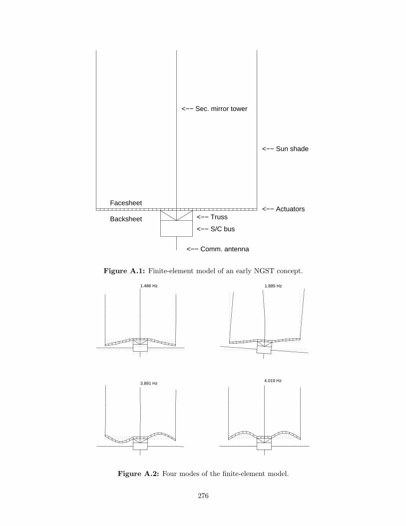
<−− Comm. antenna

<−− S/C bus

<−− Truss

<−− Sun shade

<−− Sec. mirror tower

Facesheet

Backsheet

<−− Actuators

Figure A.1: Finite-element model of an early NGST concept.

1.486 Hz 1.885 Hz

3.891 Hz4.019 Hz

Figure A.2: Four modes of the finite-element model.

276

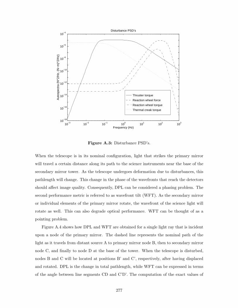
Thruster torque

Reaction wheel force

Reaction wheel torque

Thermal creak torque

10−3

10−2

10−1

100

101

102

103

10−18

10−16

10−14

10−12

10−10

10−8

10−6

10−4

Frequency (Hz)

Aut

ospe

ctra

(N

^2/H

z, (

N−m

)^2/

Hz)

Disturbance PSD’s

Figure A.3: Disturbance PSD’s.

When the telescope is in its nominal configuration, light that strikes the primary mirror

will travel a certain distance along its path to the science instruments near the base of the

secondary mirror tower. As the telescope undergoes deformation due to disturbances, this

pathlength will change. This change in the phase of the wavefronts that reach the detectors

should affect image quality. Consequently, DPL can be considered a phasing problem. The

second performance metric is referred to as wavefront tilt (WFT). As the secondary mirror

or individual elements of the primary mirror rotate, the wavefront of the science light will

rotate as well. This can also degrade optical performance. WFT can be thought of as a

pointing problem.

Figure A.4 shows how DPL and WFT are obtained for a single light ray that is incident

upon a node of the primary mirror. The dashed line represents the nominal path of the

light as it travels from distant source A to primary mirror node B, then to secondary mirror

node C, and finally to node D at the base of the tower. When the telescope is disturbed,

nodes B and C will be located at positions B’ and C’, respectively, after having displaced

and rotated. DPL is the change in total pathlength, while WFT can be expressed in terms

of the angle between line segments CD and C’D’. The computation of the exact values of

277

primary mirror

A

B’B

CC’

D’Dmirror node

sec. mirrornode

Figure A.4: Ray trace used to define DPL and WFT.

DPL and WFT involves nonlinear operations, which cannot be incorporated in the analysis

method to be described. However, small angle and small displacement approximations

permit DPL and WFT to be estimated as linear combinations of the degrees of freedom of

the mirror nodes and the secondary mirror node.

A couple of additional points should be made. Only the contributions to DPL and WFT

due to the flexible modes of the structure are considered. The effect of rigid-body motion

is neglected and assumed to be treated by the attitude control system. Also, even though

the primary mirror is modeled as a flat surface, it is assumed that the undeformed mirror

will redirect the incident light toward the secondary mirror.

Since a stochastic analysis is performed, mean-square values of DPL and WFT are

obtained for each light ray. The number of rays is equal to the number of mirror nodes,

and by averaging DPL and WFT across the mirror, a sense can be gained of the average

RMS errors.

The equations of motion of the FEM can be transformed to modal coordinates by using

a truncated set of modes from the eigensolution. These matrix equations can then be recast

in state-space form and used in a dynamic analysis. The disturbance w acts to drive the

states of the system, and the performance variable z (a vector) is a linear combination of

these states. When doing a stochastic analysis, the disturbance w can be thought of as

278

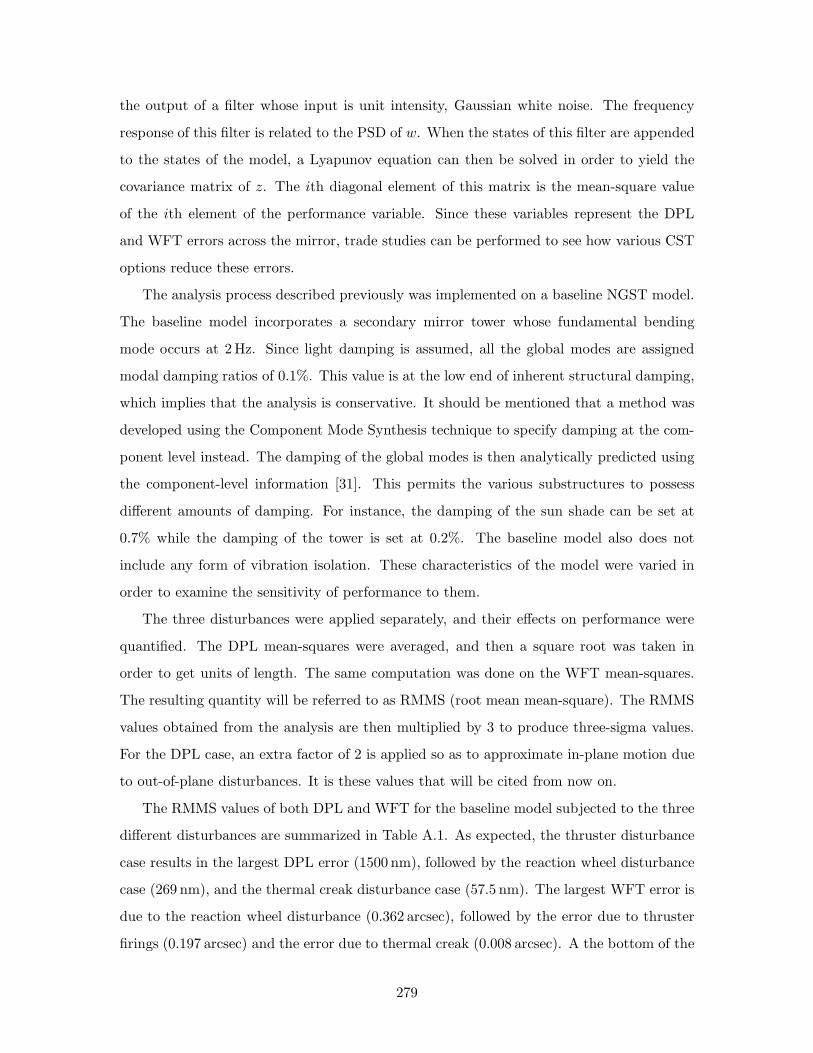
the output of a filter whose input is unit intensity, Gaussian white noise. The frequency

response of this filter is related to the PSD of w. When the states of this filter are appended

to the states of the model, a Lyapunov equation can then be solved in order to yield the

covariance matrix of z. The ith diagonal element of this matrix is the mean-square value

of the ith element of the performance variable. Since these variables represent the DPL

and WFT errors across the mirror, trade studies can be performed to see how various CST

options reduce these errors.

The analysis process described previously was implemented on a baseline NGST model.

The baseline model incorporates a secondary mirror tower whose fundamental bending

mode occurs at 2 Hz. Since light damping is assumed, all the global modes are assigned

modal damping ratios of 0.1%. This value is at the low end of inherent structural damping,

which implies that the analysis is conservative. It should be mentioned that a method was

developed using the Component Mode Synthesis technique to specify damping at the com-

ponent level instead. The damping of the global modes is then analytically predicted using

the component-level information [31]. This permits the various substructures to possess

different amounts of damping. For instance, the damping of the sun shade can be set at

0.7% while the damping of the tower is set at 0.2%. The baseline model also does not

include any form of vibration isolation. These characteristics of the model were varied in

order to examine the sensitivity of performance to them.

The three disturbances were applied separately, and their effects on performance were

quantified. The DPL mean-squares were averaged, and then a square root was taken in

order to get units of length. The same computation was done on the WFT mean-squares.

The resulting quantity will be referred to as RMMS (root mean mean-square). The RMMS

values obtained from the analysis are then multiplied by 3 to produce three-sigma values.

For the DPL case, an extra factor of 2 is applied so as to approximate in-plane motion due

to out-of-plane disturbances. It is these values that will be cited from now on.

The RMMS values of both DPL and WFT for the baseline model subjected to the three

different disturbances are summarized in Table A.1. As expected, the thruster disturbance

case results in the largest DPL error (1500 nm), followed by the reaction wheel disturbance

case (269 nm), and the thermal creak disturbance case (57.5 nm). The largest WFT error is

due to the reaction wheel disturbance (0.362 arcsec), followed by the error due to thruster

firings (0.197 arcsec) and the error due to thermal creak (0.008 arcsec). A the bottom of the

279

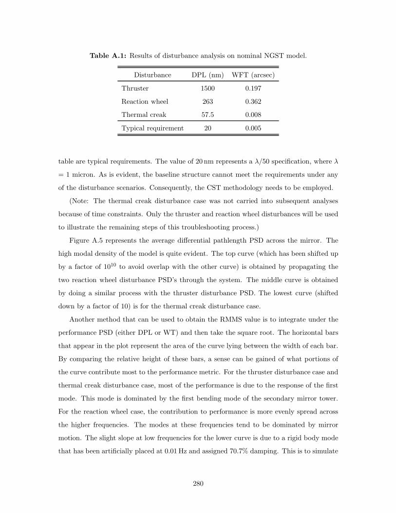
Table A.1: Results of disturbance analysis on nominal NGST model.

Disturbance DPL (nm) WFT (arcsec)

Thruster 1500 0.197

Reaction wheel 263 0.362

Thermal creak 57.5 0.008

Typical requirement 20 0.005

table are typical requirements. The value of 20 nm represents a λ/50 specification, where λ

= 1 micron. As is evident, the baseline structure cannot meet the requirements under any

of the disturbance scenarios. Consequently, the CST methodology needs to be employed.

(Note: The thermal creak disturbance case was not carried into subsequent analyses

because of time constraints. Only the thruster and reaction wheel disturbances will be used

to illustrate the remaining steps of this troubleshooting process.)

Figure A.5 represents the average differential pathlength PSD across the mirror. The

high modal density of the model is quite evident. The top curve (which has been shifted up

by a factor of 1010 to avoid overlap with the other curve) is obtained by propagating the

two reaction wheel disturbance PSD’s through the system. The middle curve is obtained

by doing a similar process with the thruster disturbance PSD. The lowest curve (shifted

down by a factor of 10) is for the thermal creak disturbance case.

Another method that can be used to obtain the RMMS value is to integrate under the

performance PSD (either DPL or WT) and then take the square root. The horizontal bars

that appear in the plot represent the area of the curve lying between the width of each bar.

By comparing the relative height of these bars, a sense can be gained of what portions of

the curve contribute most to the performance metric. For the thruster disturbance case and

thermal creak disturbance case, most of the performance is due to the response of the first

mode. This mode is dominated by the first bending mode of the secondary mirror tower.

For the reaction wheel case, the contribution to performance is more evenly spread across

the higher frequencies. The modes at these frequencies tend to be dominated by mirror

motion. The slight slope at low frequencies for the lower curve is due to a rigid body mode

that has been artificially placed at 0.01 Hz and assigned 70.7% damping. This is to simulate

280

Thruster dist. (middle)

Reaction wheel dist. (top; shifted up by factor of 1e10)

Thermal creak dist. (bottom; shifted down by factor of 10)

10−1

100

101

102

103

10−15

10−10

10−5

100

105

1010

1015

Frequency (Hz)

nm^2

/Hz

Differential Pathlength PSD

Figure A.5: DPL PSD’s.

the effect of the attitude control system.

So as to avoid confusion, performance in this context is taken to mean the RMMS values

of the WFT and DPL performance variables in z. Performance is improved whenever these

values are lowered. A statement like “Added damping improved performance” implies that

damping decreased the RMMS values of WFT and DPL.

The PSD’s in Figure A.6 correspond to the wavefront tilt component of performance.

The same trends that appeared in the DPL autospectra are evident in these plots. More

modes appear at the higher frequencies because the higher order mirror modes are charac-

terized by fairly large rotations of the mirror nodes. Consequently, wavefront tilt is affected

more than is differential pathlength.

Figure A.7 indicates the RMS value of differential pathlength for each light ray that is

incident upon a node of the primary mirror. The horizontal axis represents the position on

the mirror that the incoming light ray strikes. The thruster disturbance and thermal creak

disturbance cases have similar shapes. Both these disturbances excite the lower frequency

modes. The dominant low frequency mode is the tower bending mode. As the tower bends,

its horizontal motion contributes more to the DPL of the rays striking the outer mirror

edge than to the DPL of rays striking near the center (ignoring any blockage effects). The

281

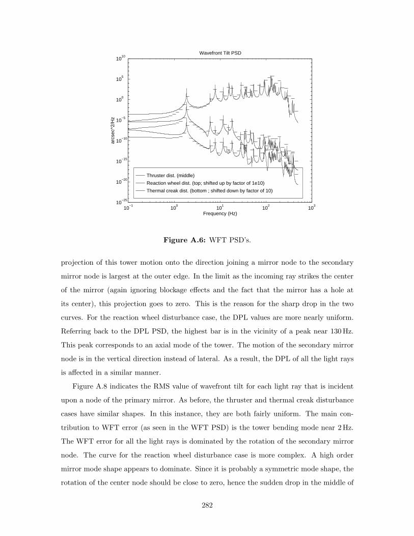
Thruster dist. (middle)

Reaction wheel dist. (top; shifted up by factor of 1e10)

Thermal creak dist. (bottom ; shifted down by factor of 10)

10−1

100

101

102

103

10−25

10−20

10−15

10−10

10−5

100

105

1010

Frequency (Hz)

arcs

ec^2

/Hz

Wavefront Tilt PSD

Figure A.6: WFT PSD’s.

projection of this tower motion onto the direction joining a mirror node to the secondary

mirror node is largest at the outer edge. In the limit as the incoming ray strikes the center

of the mirror (again ignoring blockage effects and the fact that the mirror has a hole at

its center), this projection goes to zero. This is the reason for the sharp drop in the two

curves. For the reaction wheel disturbance case, the DPL values are more nearly uniform.

Referring back to the DPL PSD, the highest bar is in the vicinity of a peak near 130 Hz.

This peak corresponds to an axial mode of the tower. The motion of the secondary mirror

node is in the vertical direction instead of lateral. As a result, the DPL of all the light rays

is affected in a similar manner.

Figure A.8 indicates the RMS value of wavefront tilt for each light ray that is incident

upon a node of the primary mirror. As before, the thruster and thermal creak disturbance

cases have similar shapes. In this instance, they are both fairly uniform. The main con-

tribution to WFT error (as seen in the WFT PSD) is the tower bending mode near 2Hz.

The WFT error for all the light rays is dominated by the rotation of the secondary mirror

node. The curve for the reaction wheel disturbance case is more complex. A high order

mirror mode shape appears to dominate. Since it is probably a symmetric mode shape, the

rotation of the center node should be close to zero, hence the sudden drop in the middle of

282

Thruster dist.

Reaction wheel dist.

Thermal creak dist.

−4 −3 −2 −1 0 1 2 3 410

−2

10−1

100

101

102

103

104

Node Position (m)

RM

S c

hang

e in

pat

hlen

gth

(nm

)

RMS Differential Pathlength vs. Position on Mirror

Figure A.7: DPL as a function of location on mirror.

the plot.

Since the baseline NGST model is unable to satisfy the performance requirements, there

is a need to identify which CST options would be particularly helpful. The usual first-

cut strategy would be to look at either structural redesign, passive vibration isolation, or

damping augmentation as potential remedies. These will be addressed in the remainder of

this demonstration in the form of sample trade studies. If no reasonable combination can

be found to help the system reach the desired performance level, then the next step would

be to look at active structural control. An example would be to extend the bandwidth of

the primary mirror actuators and/or of the tertiary fast-steering mirrors.

As mentioned previously, one parameter in the model is the frequency of the bending

mode of the tower (assuming the tower is clamped at its base). Recall from the PSD plots of

DPL and WFT for the thruster disturbance case that the performance is dominated by this

bending mode. Stiffening the tower would make the frequency of this mode higher, thereby

moving it into a region where the thruster autospectrum is rolling off and exhibiting less

influence on the modes. Physically, a stiffer tower would mean less motion of the secondary

mirror. This should reduce the amount of DPL and WFT caused by tower motion. As the

283

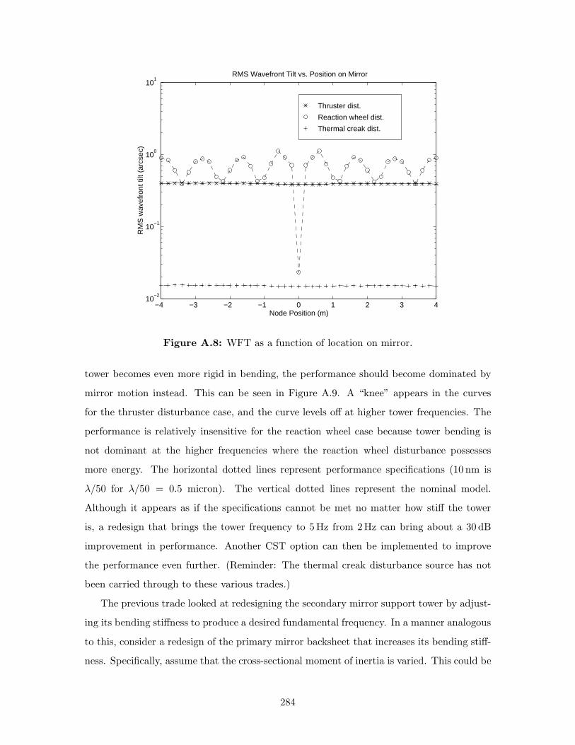
Thruster dist.

Reaction wheel dist.

Thermal creak dist.

−4 −3 −2 −1 0 1 2 3 410

−2

10−1

100

101

Node Position (m)

RM

S w

avef

ront

tilt

(arc

sec)

RMS Wavefront Tilt vs. Position on Mirror

Figure A.8: WFT as a function of location on mirror.

tower becomes even more rigid in bending, the performance should become dominated by

mirror motion instead. This can be seen in Figure A.9. A “knee” appears in the curves

for the thruster disturbance case, and the curve levels off at higher tower frequencies. The

performance is relatively insensitive for the reaction wheel case because tower bending is

not dominant at the higher frequencies where the reaction wheel disturbance possesses

more energy. The horizontal dotted lines represent performance specifications (10 nm is

λ/50 for λ/50 = 0.5 micron). The vertical dotted lines represent the nominal model.

Although it appears as if the specifications cannot be met no matter how stiff the tower

is, a redesign that brings the tower frequency to 5 Hz from 2Hz can bring about a 30 dB

improvement in performance. Another CST option can then be implemented to improve

the performance even further. (Reminder: The thermal creak disturbance source has not

been carried through to these various trades.)

The previous trade looked at redesigning the secondary mirror support tower by adjust-

ing its bending stiffness to produce a desired fundamental frequency. In a manner analogous

to this, consider a redesign of the primary mirror backsheet that increases its bending stiff-

ness. Specifically, assume that the cross-sectional moment of inertia is varied. This could be

284

Thruster dist. Reaction wheel dist.

100

101

10−3

10−2

10−1

100

0.005 arcsec

Frequency (Hz)

RM

MS

(ar

csec

)

Wavefront Tilt vs. Tower Freq.

100

101

101

102

103

104

10 nm

20 nm

RM

MS

(nm

)

Diff. Pathlength vs. Tower Freq.

Frequency (Hz)

Figure A.9: Tower frequency trade study.

accomplished by varying the backsheet from a thin sheet, to a sandwich-honeycomb struc-

ture, to a truss support structure. The performance plots for this trade in Figure A.10 do

not show recognizable trends. In all instances, the required performance cannot be achieved.

For the thruster disturbance case, the lack of improvement can be explained as follows. The

mode responsible for the largest contribution to the performance metric is the fundamental

bending mode of the tower. The tower is modeled as being clamped to the backsheet. As

the stiffness of this backsheet changes, the frequency of the global mode characterized by

tower bending will change to an extent that depends on the degree of coupling. However,

the frequency shift is not substantial. Since the roll-off region of the thruster disturbance

PSD occurs in the vicinity of this mode, the contribution to performance will depend on

where the mode is relative to the roll-off. This can explain the relative insensitivity of DPL

and WFT to backsheet stiffness. Put another way, the DPL and WFT RMMS values will

still be dominated by tower motion, no matter how stiff the backsheet is. Probably the

next step that should be performed is to repeat this trade, but for the case of a 5 Hz tower.

(Remember, this trade is for the nominal design, which has a 2Hz tower.) Mirror motion

should comprise more of the performance in that case.

For the reaction wheel disturbance case, the same kind of relative insensitivity is ap-

parent. A possible reason for this is that the low order mirror modes are being shifted up

in frequency. These modes previously were not in the frequency region of largest reaction

285

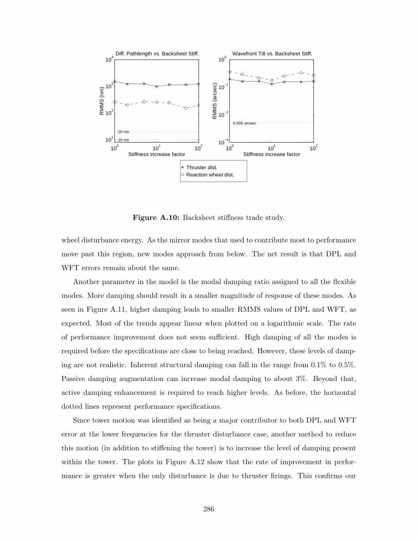
Thruster dist. Reaction wheel dist.

100

101

102

10−3

10−2

10−1

100

0.005 arcsec

Stiffness increase factor

RM

MS

(ar

csec

)

Wavefront Tilt vs. Backsheet Stiff.

100

101

102

101

102

103

104

10 nm

20 nm

Stiffness increase factor

RM

MS

(nm

)

Diff. Pathlength vs. Backsheet Stiff.

Figure A.10: Backsheet stiffness trade study.

wheel disturbance energy. As the mirror modes that used to contribute most to performance

move past this region, new modes approach from below. The net result is that DPL and

WFT errors remain about the same.

Another parameter in the model is the modal damping ratio assigned to all the flexible

modes. More damping should result in a smaller magnitude of response of these modes. As

seen in Figure A.11, higher damping leads to smaller RMMS values of DPL and WFT, as

expected. Most of the trends appear linear when plotted on a logarithmic scale. The rate

of performance improvement does not seem sufficient. High damping of all the modes is

required before the specifications are close to being reached. However, these levels of damp-

ing are not realistic. Inherent structural damping can fall in the range from 0.1% to 0.5%.

Passive damping augmentation can increase modal damping to about 3%. Beyond that,

active damping enhancement is required to reach higher levels. As before, the horizontal

dotted lines represent performance specifications.

Since tower motion was identified as being a major contributor to both DPL and WFT

error at the lower frequencies for the thruster disturbance case, another method to reduce

this motion (in addition to stiffening the tower) is to increase the level of damping present

within the tower. The plots in Figure A.12 show that the rate of improvement in perfor-

mance is greater when the only disturbance is due to thruster firings. This confirms our

286

Thruster dist. Reaction wheel dist.

.1% 1% 10%10

−3

10−2

10−1

100

0.005 arcsec

Zeta (damping ratio)

RM

MS

(ar

csec

)

Wavefront Tilt vs. Global Damping

.1% 1% 10%10

1

102

103

104

10 nm

20 nm

Zeta (damping ratio)

RM

MS

(nm

)

Diff. Pathlength vs. Global Damping

Figure A.11: Modal damping trade study.

intuition. The effect of damping appears linear in these logarithmic plots, and the slope is

shallower for the reaction wheel disturbance case. This again matches previous statements

regarding the effect of tower motion on performance when the system is excited by reaction

wheel chatter. The level of performance at even high amounts of tower damping is still

not near the desired specification. This suggests that adding large quantities of damping

treatments, which come at the cost of extra mass and complexity (for active damping), is

not worthwhile.

Since mirror motion was identified as contributing to both DPL and WFT error at the

higher frequencies for the reaction wheel disturbance case, adding damping to the mirror

will aid in reducing these errors. Figure A.13 confirms this statement. However, the amount

of damping required to yield substantial performance improvement is in the active damping

range. Mirror damping appears to affect WFT error more than DPL error. Going from

0.1% damping to 10% damping only reduces DPL RMMS by a factor of 3, while it reduces

WFT RMMS by a factor of 10. The plots also confirm that mirror damping has no effect

on performance when the system is being excited by thruster firings. This is because the

dominant mode in this case has little mirror motion.

This trade and the previous trade indicate that:

• the tower should be damped if the predominant disturbance source is due to thrusters

287

Thruster dist. Reaction wheel dist.

.1% 1% 10%10

−3

10−2

10−1

100

0.005 arcsec

Zeta (damping ratio)

RM

MS

(ar

csec

)

Wavefront Tilt vs. Tower Damping

.1% 1% 10%10

1

102

103

104

10 nm

20 nm

Zeta (damping ratio)

RM

MS

(nm

)

Diff. Pathlength vs. Tower Damping

Figure A.12: Tower modal damping trade study.

• the mirror should be damped if the predominant disturbance source is due to reaction

wheel noise

Isolation in the truss that serves as the interface between the spacecraft (where the

disturbances enter) and the mirror assembly (where the performance is affected) is one

common method used to attenuate the transmission of vibrations. One characteristic of

an isolator is its so-called “corner” frequency. The plots in Figure A.14 show how the

performance can be improved by decreasing this frequency. Passive isolation was added

to the model by reducing both the extensional stiffness and bending stiffness of the truss

members, and by setting the truss damping to an arbitrary level of 20%. The bending

destiffening was required in order to avoid “blocking zeros” which arise when a cross-axis

stiffness limits the performance of an isolator [38]. A soft truss leads to three additional

modes that are dominated by motion of the truss. The highest frequency of these modes

will be considered an indication of the corner frequency. A moderate corner frequency is

required to meet the performance specifications for the reaction wheel disturbance case.

An extremely low corner frequency is required for the thruster disturbance case. This is

probably due to the fact that the corner frequency should be below the frequencies of the

modes contributing to the performance. In this case, the problematic mode is the tower

bending mode near 2 Hz.

288

Thruster dist. Reaction wheel dist.

.1% 1% 10%10

−3

10−2

10−1

100

0.005 arcsec

Zeta (damping ratio)

RM

MS

(ar

csec

)

Wavefront Tilt vs. Mirror Damping

.1% 1% 10%10

1

102

103

104

10 nm

20 nm

Zeta (damping ratio)

RM

MS

(nm

)

Diff. Pathlength vs. Mirror Damping

Figure A.13: Mirror modal damping trade study.

Thruster dist. Reaction wheel dist.

100

101

10−3

10−2

10−1

100

0.005 arcsec

Frequency (Hz)

RM

MS

(ar

csec

)

Wavefront Tilt vs. Isolator Freq.

100

101

100

101

102

103

104

10 nm

20 nmRM

MS

(nm

)

Diff. Pathlength vs. Isolator Freq.

Frequency (Hz)

Figure A.14: Isolator corner frequency trade study.

289

Table A.2: Comparison of use of controlled structures technologies.

CST option Helpful? Amount Needed Feasible?

Stiffer tower Yes, for thrusterdisturbance case

Cannot achieverequirements

—

Increased globaldamping

Yes Must be > 50% No

Increased towerdamping

More so forthrusterdisturbance

Cannot achieverequirements

—

Isolation Yes Thruster dist.:40 dB, 0.2 Hz,20% damping

Not likely

RWA dist.:30 dB, 2 Hz, 20%damping

Yes

Based on the trends that appear in the previous plots, estimates can be made of how

much of each CST option would be required to satisfy the performance requirements (as-

suming it is the only option implemented). Table A.2 summarizes the findings. For each

option, comments are made regarding how helpful it is to performance enhancement, how

much would be required to meet the requirements (if possible), and how feasible this amount

would be.

The results can be summarized as follows:

• Increasing the bending stiffness of the tower does help quite a bit for the thruster

disturbance case, yet it cannot alone bring the DPL and WFT values down to the

desired level.

• Increasing overall damping is also helpful, but the rate of performance improvement

is not fast enough to make the required amount of global damping feasible. Not even

50% modal damping for all the modes is sufficient to achieve both DPL and WFT

specifications.

• Increasing tower damping is more effective in reducing errors due to thruster firings;

however, no amount of damping can cause the desired performance to be met for both

290

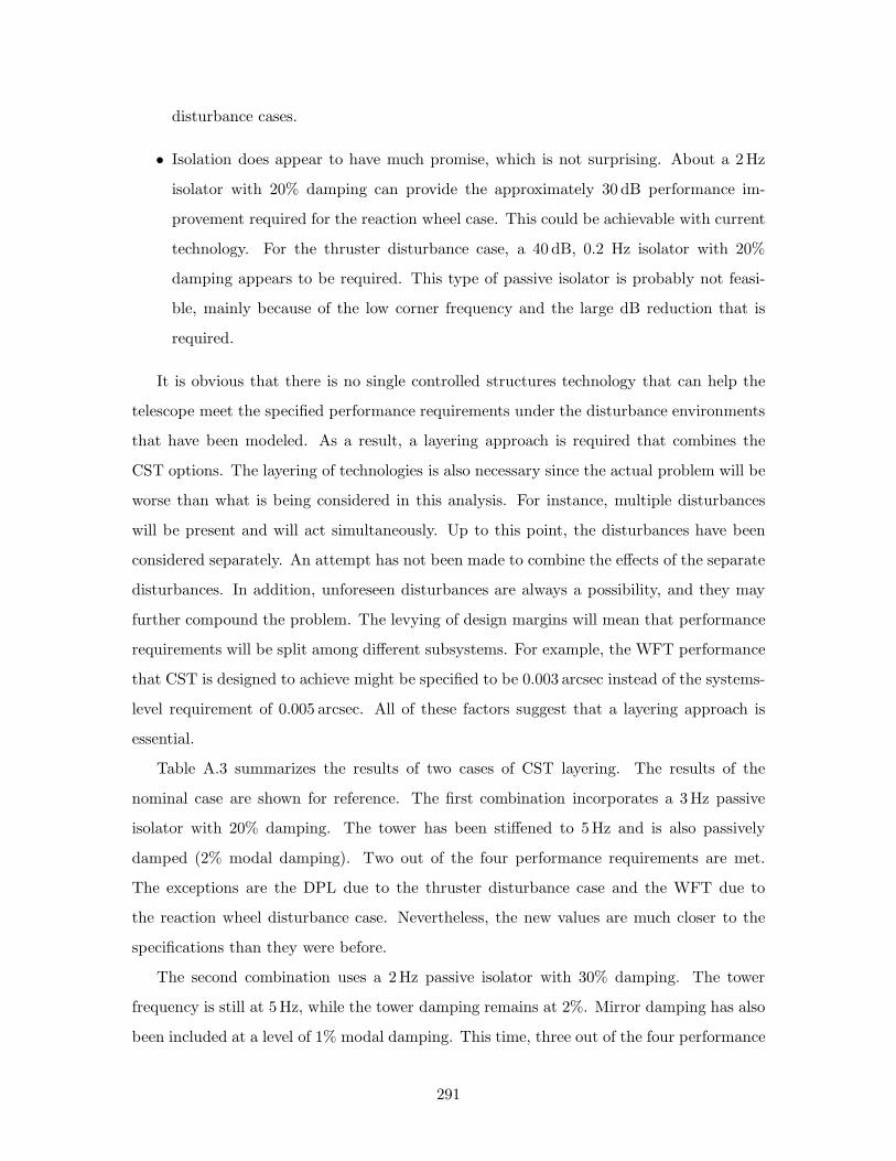
disturbance cases.

• Isolation does appear to have much promise, which is not surprising. About a 2Hz

isolator with 20% damping can provide the approximately 30 dB performance im-

provement required for the reaction wheel case. This could be achievable with current

technology. For the thruster disturbance case, a 40 dB, 0.2 Hz isolator with 20%

damping appears to be required. This type of passive isolator is probably not feasi-

ble, mainly because of the low corner frequency and the large dB reduction that is

required.

It is obvious that there is no single controlled structures technology that can help the

telescope meet the specified performance requirements under the disturbance environments

that have been modeled. As a result, a layering approach is required that combines the

CST options. The layering of technologies is also necessary since the actual problem will be

worse than what is being considered in this analysis. For instance, multiple disturbances

will be present and will act simultaneously. Up to this point, the disturbances have been

considered separately. An attempt has not been made to combine the effects of the separate

disturbances. In addition, unforeseen disturbances are always a possibility, and they may

further compound the problem. The levying of design margins will mean that performance

requirements will be split among different subsystems. For example, the WFT performance

that CST is designed to achieve might be specified to be 0.003 arcsec instead of the systems-

level requirement of 0.005 arcsec. All of these factors suggest that a layering approach is

essential.

Table A.3 summarizes the results of two cases of CST layering. The results of the

nominal case are shown for reference. The first combination incorporates a 3Hz passive

isolator with 20% damping. The tower has been stiffened to 5Hz and is also passively

damped (2% modal damping). Two out of the four performance requirements are met.

The exceptions are the DPL due to the thruster disturbance case and the WFT due to

the reaction wheel disturbance case. Nevertheless, the new values are much closer to the

specifications than they were before.

The second combination uses a 2Hz passive isolator with 30% damping. The tower

frequency is still at 5 Hz, while the tower damping remains at 2%. Mirror damping has also

been included at a level of 1% modal damping. This time, three out of the four performance

291

Table A.3: Results of CST Layering.

CST Layered Design DPL (nm) WFT (arcsec)

Thruster RWA Thruster RWA

Nominal design 1500 263 0.197 0.362

Isolator (3 Hz, 20% damp.)5Hz tower2% tower damp.

32.6 6.24 0.0042 0.0063

Isolator (2 Hz, 30% damp.)5Hz tower2% tower damp., 1% mirrordamp.

25.1 5.27 0.0032 0.0026

Typical requirement 20 .005

requirements are met. The exception is the DPL for the thruster disturbance case, but this

time it is closer to meeting the 20 nm level. It is within 25% of the desired value.

It is anticipated that a few more iterations like this will lead to a reasonable design that

can meet all the requirements for both disturbance cases. However, as mentioned before,

the actual problem faced could be much worse due to several simultaneous disturbances. As

a result, some form of active control would need to be investigated. An advantage of active

control is that it can be redesigned while on-orbit (by uplinking reconfigured software) in

order to account for any unforeseen or mismodeled disturbances. This adaptive ability is

highly desirable, but with any active system there is the chance for instability, so care must

be taken.

A number of additional studies can be done that build upon the results obtained thus

far. Further trade studies can be performed to examine the effect on performance of a

variety of other design parameters. The issue of the use of active structural control needs

to be addressed (for the reasons discussed previously). Besides the NGST point design that

has been modeled, alternative structural architectures can be studied using this analysis

methodology. Finally, a traditional sensitivity analysis can be performed.

Sensitivity analysis is an attractive method for a number of reasons. What it provides is

an indication of how changes made to model parameters affect a cost functional or perfor-

mance metric that has been defined. Essentially, it can provide the slope of a performance

292

vs. parameter curve at a nominal value of the parameter. A steep slope indicates that

the performance is very sensitive to the parameter; consequently, that parameter should be

considered as a possible design variable. A sensitivity analysis can be more efficient than

performing the process manually, as was done to create the performance vs. parameter

curves shown previously. The “manual” process involves changing the parameter of inter-

est, rerunning the dynamic analysis, and then seeing what the value of performance is. This

is then repeated for another value of the parameter.

The parameter sensitivities can reveal which model parameters provide more “bang for

the buck.” For example, if a 1% change in component stiffness produces the same effect as

a factor of 100 increase in component damping, then obviously the stiffness redesign should

be implemented instead. Once a series of parameter sensitivities has been determined (and

properly normalized), then an optimization routine can be employed that identifies what

combination of parameters will minimize and hopefully satisfy the performance metric. This

can then aid in allocating requirements to the different CST options.

The example jitter analysis that was conducted showed that the performance of the

nominal NGST finite-element model exceeded typical requirements on wavefront tilt and

differential pathlength by factors of 10 to 100. Since no single controlled structures tech-

nology option could realistically satisfy the performance specifications, this indicated that

a layered CST approach was required. After analyzing the impact of a number of different

options (structural redesign, passive damping, passive isolation) on the performance, a few

sample combinations were shown to be particularly effective.

What should be taken from this demonstration is not the actual numbers that resulted

from the analysis, but rather a sense of the usefulness of this approach. This analysis tool

allows early insights into redesigns and technology applications that can lead to favorable

results. It also permits early partitioning of subsystem requirements based on the available

information rather than ad hoc allocation. As more up-to-date information is gathered, the

structural, disturbance, and performance models can be updated. The analysis tool evolves

along with the design of the system. The two should go hand-in-hand, with one helping to

steer the direction of the other. This approach should be considered essential because as

results of systems trades are arrived at during the early conceptual design stages, solutions

and remedies can be incorporated in a cost-effective manner.

293

294

Appendix B

Derivation of RWA Disturbance

Cross-Spectral Density Function

We consider the case when p = q and (r, s) ∈ [(1, 2), (2, 1), (4, 5), (5, 4)] and rewrite

Eq. 2.33 accordingly.

Rwmprwmps(t1, t2) = E

[nr∑

k=1

ns∑l=1

CrkCslf4p

2cos (2πfp(hrkt1 − hslt2) + φprk − φpsl) (B.1)

− cos (2πfp(hrkt1 + hslt2) + φprk + φpsl)]

Using an argument similar to that expressed in Eq. 2.38, we notice that the expectation of

the cosine terms with φprk +φpsl will be zero (since it is never assumed that φprk +φpsl can

equal zero). In addition, the expectation of cosine terms with φprk − φpsl will vanish unless

the relationship expressed by Eq. 2.22 holds. Thus, the previous expression simplifies to

Rwmprwmps(t1, t2) = E

[nr∑

k=1

CrkCskf4p

2

cos

(2πfp(hrkt1 − hskt2)± π

2

)],

+ , r > s

− , r < s

(B.2)

Another assumption is that for the (r, s) pairs being considered in this case, hrk = hsk and

Crk = Csk. This leads to

Rwmprwmps(t1, t2) = E

[nr∑

k=1

C2rkf

4p

2cos

(2πfphrk(t1 − t2)± π

2

)],

+ , r > s

− , r < s(B.3)

But because of the identity cos(A± π2 ) = ∓sinA, this can be rewritten as

Rwmprwmps(t1, t2) = ∓E

[nr∑

k=1

C2rkf

4p

2sin (2πfphrk(t1 − t2))

],

− , r > s

+ , r < s(B.4)

295

Bringing the expectation operator within the summation and letting τ = t1 − t2,

Rwmprwmps(τ) = ∓

nr∑k=1

C2rk

2E[f4

p sin (2πfphrkτ)],

− , r > s

+ , r < s(B.5)

Now invoking the definition of the expectation operator,

Rwmprwmps(τ) = ∓

nr∑k=1

C2rk

2

∫ +∞

−∞fFP

(fp)f4p sin (2πfphrkτ) dfp,

− , r > s

+ , r < s(B.6)

Taking the Fourier transform of Eq. B.6 and noting that the Fourier transform of a sine

is a pair of impulses at the frequency of the sine (one with amplitude jπ and the other of

amplitude −jπ) [8],

Swmprwmps(ω) = ∓

nr∑k=1

C2rk

2

∫ +∞

−∞fFP

(fp)f4p

∫ +∞

−∞sin (2πfphrkτ) e−jωτdτdfp (B.7)

= ∓nr∑

k=1

C2rk

2

∫ +∞

−∞fFP

(fp)f4p jπ [δ(ω + 2πfphrk)− δ(ω − 2πfphrk)] dfp

Now make the substitutions

u1 = ω + 2πfphrk ⇒ du1 = 2πhrkdfp

u2 = ω − 2πfphrk ⇒ du2 = −2πhrkdfp

to obtain

Swmprwmps(ω) = ∓

nr∑k=1

jπC2rk

2

[∫ +∞

−∞fFP

(u1 − ω2πhrk

)(u1 − ω2πhrk

)4

δ(u1)(

12πhrk

)du1 (B.8)

+∫ +∞

−∞fFP

(−u2 + ω

2πhrk

)(−u2 + ω

2πhrk

)4

δ(u2)( −1

2πhrk

)du2

]

The integral of the product of a function and a delta function with respect to the argument

of the delta function is simply the value of the function evaluated at zero.

Swmprwmps(ω) = ∓

nr∑k=1

jπC2rk

2

[fFP

( −ω2πhrk

)( −ω2πhrk

)4 ( 12πhrk

)(B.9)

+fFP

(ω

2πhrk

)(ω

2πhrk

)4 ( −12πhrk

)]

This can be further simplified to obtain

Swmprwmps(ω) = ∓

nr∑k=1

jπC2rkω

4

2(2πhrk)5

[fFP

(ω

2πhrk

)+ fFP

( −ω2πhrk

)],

− , r > s

+ , r < s

(B.10)

At this point, no further steps can be made until a specific probability density function is

assumed for fFP(fp).

296

Appendix C

Derivation of Curvature Equation

Chapter 4 obtained the following expression for the derivative of the ith performance

variance, σ2zi

, with respect to a generic parameter p. (See Eq. 4.22.)

∂σ2zi

∂p= trace

[Σq

∂(CTi Ci)∂p

]+ trace

[Li

(∂Azd

∂pΣq + Σq

∂ATzd

∂p+∂(BzdB

Tzd)

∂p

)](C.1)

where Σq is the solution to

AzdΣq + ΣqATzd +BzdB

Tzd = 0 (C.2)

and Li is the solution to

LiAzd +ATzdLi + CT

i Ci = 0 (C.3)

We seek now to determine the curvature of σ2zi

with respect to p. In other words, we wish

to compute the second derivative∂2σ2

zi∂p2 . We can follow the same procedure as that used

in Section 4.2 to obtain the sensitivity equation. First, create the Lagrangian of∂σ2

zi∂p by

augmenting the constraint equations given by Eq. C.2 and Eq. C.3 with Lagrange multiplier

matrices Mi,p and Ni,p. These are dependent not only on the performance metric of interest,

but also the parameter of interest.(∂σ2

zi

∂p

)∗=

∂σ2zi

∂p+ trace

[Mi,p

(LiAzd +AT

zdLi +CTi Ci

)]+ trace

[Ni,p

(AzdΣq + ΣqA

Tzd +BzdB

Tzd

)](C.4)

The derivative of∂σ2

zi∂p with respect to p is equal to the derivative of the Lagrangian function

if and only if the derivatives with respect to Σq, Li, Mi,p, and Ni,p are equal to zero.

∂2σ2zi

∂p2=∂2(σ2

zi

)∗∂p2

∣∣∣∣∣∣∂(σ2zi)

∗

∂Σq=0,

∂(σ2zi)

∗

∂Li

=0,∂(σ2

zi)∗

∂Mi,p

=0,∂(σ2

zi)∗

∂Ni,p

=0

(C.5)

297

∂(σ2zi

)∗∂Li

= 0 and∂(σ2

zi)∗

∂Σq= 0 simply recover Eq. C.2 and Eq. C.3, respectively. The derivative

of Eq. C.4 with respect to Li produces

∂(σ2

zi

)∗∂Li

= Mi,pATzd +AzdMi,p

+∂Azd

∂pΣq + Σq

∂ATzd

∂p+∂(BT

zdBzd)∂p

= 0 (C.6)

This is another Lyapunov equation and is used to determine Mi,p. The derivative of Eq. C.4

with respect to Σq produces

∂(σ2

zi

)∗∂Σq

= Ni,pAzd +ATzdNi,p

+∂AT

zd

∂pLi + Li

∂Azd

∂p+∂(CiC

Ti )

∂p= 0 (C.7)

which is a Lyapunov equation used to determine Ni,p. The final equation for the curvature

of σ2zi

with respect to p is

∂2σ2zi

∂p2= trace

[Σq

∂2(CTi Ci)

∂p2

]

+ trace

[Li

(∂2Azd

∂p2Σq + Σq

∂2ATzd

∂p2+∂2(BzdB

Tzd)

∂p2

)]

+ trace

[Mi,p

(∂AT

zd

∂pLi + Li

∂Azd

∂p+∂(CT

i Ci)∂p

)]

+ trace

[Ni,p

(∂Azd

∂pΣq + Σq

∂ATzd

∂p+∂(BzdB

Tzd)

∂p

)](C.8)

where Σq, Li, Mi,p, and Ni,p are obtained from Eq. C.2, Eq. C.3, Eq. C.6, and Eq. C.7,

respectively.

Table C.1 indicates the number of Lyapunov equations that must be solved when com-

puting sensitivities and curvatures. The total number of performance metrics is nz and the

total number of parameters of interest is np. The size of Azd is ns × ns. The computa-

tional cost greatly increases when curvature information is desired. An additional 2nznp

Lyapunov equations need to be solved, and this can be an important issue for large-order

systems with several performance variables and parameters.

A “normalized” curvature of the performance RMS value with respect to p can be

computed as follows. First, write the variance sensitivity in terms of the RMS sensitivity.

∂σ2zi

∂p= 2σzi

∂σzi

∂p(C.9)

298

Table C.1: Number of Lyapunov equations needed for exact sensitivity and cur-vature calculations.

Calculation Comments # of order ns Lyap. equations

Sensitivity • 1 order ns Lyap. equation to obtainnominal Σq

• 1 order ns Lyap. equation to obtainLi for each zi

1 + nz

Curvature • 1 order ns Lyap. equation to obtainnominal Σq

• 1 order ns Lyap. equation to obtainLi for each zi

• 1 order ns Lyap. equation to obtainMi,p for each zi and p

• 1 order ns Lyap. equation to obtainNi,p for each zi and p

1 + nz(1 + 2np)

Now take another derivative with respect to p and use the chain rule.

∂2σ2zi

∂p2= 2

(∂σzi

∂p

)2

+ 2σzi

∂2σzi

∂p2(C.10)

Solving for the curvature of the RMS value leads to

∂2σzi

∂p2=

12σzi

[∂2σ2

zi

∂p2− 2

(∂σzi

∂p

)2]

(C.11)

Multiplying through by p2

σzi

to make the curvature dimensionless results in

p2

σzi

∂2σzi

∂p2=

p2

2σ2zi

∂2σ2zi

∂p2−(p

σzi

∂σzi

∂p

)2 (C.12)

Now divide through by the normalized sensitivity to obtain the normalized curvature.

1(p

σzi

∂σzi∂p

) [ p2

σzi

∂2σzi

∂p2

]

︸ ︷︷ ︸normalized curv.

=1(

pσzi

∂σzi∂p

)︸ ︷︷ ︸

normalized sens.

p2

2σ2zi

∂2σ2zi

∂p2−

(p

σzi

∂σzi

∂p

)2

︸ ︷︷ ︸normalized sens.

(C.13)

299

The left-hand side of the equation can be approximated by

∆

(p

σzi

∂σzi∂p

)p

σzi

∂σzi∂p

∆pp

=% change in normalized sensitivity

% change in parameter p(C.14)

which can be thought of as a normalized curvature value.

A large value indicates that the sensitivity changes rapidly for small parameter values.

A small value, on the other hand, suggests that the sensitivity is relatively constant and

first-order approximations can be used to a good degree of accuracy.

300

References

[1] K. J. Astrom and B. Wittenmark, Computer-Controlled Systems: Theory andDesign, Prentice-Hall, Inc., 1997.

[2] M. Athans, Lecture notes for Multivariable Control Systems II, MIT course 6.234J,January 1995.

[3] Ball Aerospace and Technologies Corporation, Electro-Optical Line-of-SightControls, URL <http://www.ball.com/aerospace/ptlos.html>. Accessed December 5,1998.

[4] Ball Aerospace and Technologies Corporation, Gimbal Designs. URL<http://www.ball.com/aerospace/gimbals.html>. Accessed December 5, 1998.

[5] K. J. Bathe, Finite Element Procedures, Prentice-Hall, Inc., 1996.

[6] B. Bialke, A compilation of reaction wheel induced spacecraft disturbances, in Pro-ceedings of the 20th Annual AAS Guidance and Control Conference, Breckenridge,CO, February 5–9, 1997. AAS Paper No. 97-038.

[7] G. H. Blackwood, R. N. Jacques, and D. W. Miller, The MIT multipointalignment testbed: technology development for optical interferometry, in Proceedings ofthe SPIE Conference on Active and Adaptive Optical Systems, vol. 1542, San Diego,CA, July 1991, pp. 371–391.

[8] R. G. Brown and P. Y. C. Hwang, Introduction to Random Signals and AppliedKalman Filtering, John Wiley & Sons, Inc., 1997.

[9] A. E. Bryson and R. A. Mills, Linear-quadratic-gaussian controllers with specifiedparameter robustness, Journal of Guidance, Control, and Dynamics, 21 (1998), pp. 11–18.

[10] M. E. Campbell and E. F. Crawley, Development of structural uncertainty models,Journal of Guidance, Control, and Dynamics, 20 (1997), pp. 841–849.

[11] M. Colavita, Visibility and phasing, JPL Interoffice Memorandum, To SITE distri-bution, August 10, 1994.

[12] R. D. Cook, D. S. Malkus, and M. E. Plesha, Concepts and Applications ofFinite Element Analysis, John Wiley & Sons, Inc., 1989.

[13] R. Craig Jr., Structural Dynamics: An Introduction to Computer Methods, JohnWiley & Sons, Inc., 1981.

[14] S. H. Crandall and W. D. Mark, Random Vibration in Mechanical Systems, Aca-demic Press, 1963.

[15] E. F. Crawley, B. P. Masters, and T. T. Hyde, Conceptual design methodol-

301

ogy for high performance dynamic structures, in Proceedings of the 36th AIAA Struc-tures, Structural Dynamics, and Materials Conference, New Orleans, LA, April 1995,pp. 2768–2787. AIAA Paper No. 95-2557.

[16] L. P. Davis, D. Cunningham, and J. Harrell, Advanced 1.5 Hz passive viscousisolation system, in Proceedings of the 35th AIAA/ASME/ASCE/AAS/ASC Struc-tures, Structural Dynamics, and Materials Conference, Hilton Head, SC, April 18–24,1994, pp. 2655–2665. AIAA Paper No. 94-1651.

[17] L. P. Davis, J. F. Wilson, R. E. Jewell, and J. J. Roden, Hubble space telescopereaction wheel assembly vibration isolation system, in Vibration Damping Workshop,Marshall Space Flight Center, March 1986.

[18] O. de Weck, D. Miller, and H. Gutierrez, Structural dynamics and controls forNGST, in Proceedings of the 34th Liege International Astrophysics Colloquium, Liege,Belgium, June 15–18, 1998.

[19] L. E. El Ghaoui and A. E. Bryson, Wost parameter changes for stabilized conser-vative systems, in AIAA Guidance, Navigation, and Control Conference, New Orleans,LA, 1991, pp. 1490–1495.

[20] C. E. Eyerman and J. F. Shea, A systems engineering approach to disturbance min-imization for spacecraft utilizing controlled structures technology, MIT SERC Report#2-90, June 1990.

[21] R. L. Fox and M. P. Kapoor, Rates of change of eigenvalues and eigenvectors,AIAA Journal, 6 (1968), pp. 2426–2429.

[22] G. F. Franklin and J. D. Powell, Digital Control of Dynamic Systems, Addison-Wesley Publishing Co., Inc., 1980.

[23] B. Friedland, Control System Design: An Introduction to State-Space Methods,McGraw-Hill, Inc., 1986.

[24] A. Gelb, ed., Applied Optimal Estimation, The M.I.T. Press, 1974.

[25] R. M. Glaese, Impedance Matching for Structural-Acoustic Conrol, PhD thesis, Mas-sachusetts Institute of Technology, April 1997. SERC Report #2-97.

[26] A. Grace, Optimization Toolbox User’s Guide, The MathWorks, Inc., 1994.

[27] C. Z. Gregory, Reduction of large flexible spacecraft models using internal balancingtheory, Journal of Guidance, Control, and Dynamics, 7 (1984), pp. 17–32.

[28] S. C. O. Grocott, Comparision of control techniques for robust performance onuncertain structural systems, Master’s thesis, Massachusetts Institute of Technology,January 1994. SERC Report #2-94.

[29] R. L. Grogan and R. A. Laskin, On multidisciplinary modeling of the space inter-ferometry mission, in Proceedings of the American Control Conference, Philadelphia,PA, June 1998.

[30] H. Gutierrez, M. Levine, and R. Grogan, Analysis of IPEX-2 pre-flight groundintegration test data, Tech. Rep. D-14905, NASA Jet Propulsion Laboratory, October1997.

[31] H. L. Gutierrez, Damping formulations in substructure synthesis, Master’s thesis,Massachusetts Institute of Technology, May 1994.

302

[32] H. L. Gutierrez and D. W. Miller, Disturbance analysis of integrated struc-tural/optical models with uncertainties, in Proceedings of the American Control Con-ference, Philadelphia, PA, June 1998.

[33] T. K. Hasselman, J. D. Chrostowski, and T. J. Ross, Interval predictionin structural dynamic analysis, in Proceedings of the 33rd AIAA/ASME/AHS/ASCStructures, Structural Dynamics, and Materials Conference, Dallas, TX, April 1992,pp. 1272–1284. AIAA Paper No. 92-2215.

[34] , Propagation of modeling uncertainty through structural dynamic models, in Pro-ceedings of the 35th AIAA/ASME/AHS/ASC Structures, Structural Dynamics, andMaterials Conference, Hilton Head, SC, April 1994.

[35] G. J. Hou and S. P. Kenny, Eigenvalue and eigenvector approximate analysis forrepeated eigenvalue problems, AIAA Journal, 30 (1992).

[36] G. J. Hou and G. Koganti, Sensitivity analysis of Lyapunov and Ricaati equa-tions with application to controls-structures integrated design, in Proceedings of the34th AIAA/ASME/ASCE/AHS/ASC Structures, Structural Dynamics and MaterialsConference, LaJolla, CA, April 1993, pp. 1906–1915. AIAA Paper No. 93-1529.

[37] J. P. How, Robust Control Design with Real Parameter Uncertainty Using AbsoluteStability Theory, PhD thesis, Massachusetts Institute of Technology, February 1993.SERC Report #1-93.

[38] T. T. Hyde, Active Vibration Isolation for Precision Space Structures, PhD thesis,Massachusetts Institute of Technology, January 1996. SERC Report #4-96.

[39] M. Ingham, Microdynamics and thermal snap response of deployable space structures,Master’s thesis, Massachusetts Institute of Technology, June 1998. SERC Report #2-98.

[40] R. N. Jacques, An approach to the preliminary design of controlled structures, Mas-ter’s thesis, Massachusetts Institute of Technology, February 1991. SERC Report #1-91.

[41] , On-line System Identification and Control Design for Flexible Structures, PhDthesis, Massachusetts Institute of Technology, May 1995. SERC Report #3-95.

[42] L. Jandura, Analysis of hexapod isolator requirements necessary to meet SIMOPD requirements for astrometry and nulling, Interoffice Memorandum SIM/ITPLJAN9705151, Jet Propulsion Laboratory, May 15, 1997.

[43] Jet Propulsion Laboratory, Origins Missions, URL<http://origins.jpl.nasa.gov/missions/sbobs.html>. Accessed November 29, 1998.

[44] Jet Propulsion Laboratory, Space Interferometry Mission, URL<http://huey.jpl.nasa.gov/sim/index.html>. Accessed November 11, 1998.

[45] Jet Propulsion Laboratory, Modeling and Analysis for Controlled Optical SystemsUser’s Manual, 1997.

[46] , Integrated Modeling of Optical Systems User’s Manual, January 1998. JPL D-13040.

[47] A. J. Keane and A. P. Bright, Passive vibration control via unusual geome-tries: Experiments on model aerospace structures, Journal of Sound and Vibration,192 (1996).

303

[48] S. Kenny, Eigenvalue and eigenvector derivatives for structures, Final Report, MITCourse 2.093: Computer Methods in Dynamics, April 29,1997.

[49] Y. Kim, Thermal Creak Induced Dynamics of Space Structures, PhD thesis, Mas-sachusetts Institute of Technology, February 1999. SERC Report #14-98.

[50] W. J. Larson and J. R. Wertz, eds., Space Mission Analysis and Design, Micro-cosm, Inc. and Kluwer Academic Publishers, 1991.

[51] R. A. Laskin, Technology for space optical interferometry, in Proceedings of the 33rd

AIAA Aerospace Science Meeting and Exhibit, Reno, NV, January 1995. AIAA PaperNo. 95-0825.

[52] R. A. Laskin, SIM Dynamics & Control Requirements Flowdown Process. Presenta-tion at the SIM Project Preliminary Instrument System Requirements Review, JPL,March 17–18, 1998.

[53] R. A. Laskin and M. San Martin, Control/structure system design of a space-borne optical interferometer, in Proceedings of the AAS/AIAA Astrodynamics Spe-cialist Conference, Stowe, VT, August 1989. AAS Paper No. 89-424.

[54] M. Levine, R. Bruno, and H. Gutierrez, Interferometry program flight experiment#1: Objectives and results, in Proceedings of the 16th International Modal AnalysisConference, Santa Barbara, CA, 1998, pp. 1184–1190.

[55] M. B. Levine, Interferometry program flight experiments: IPEX I and II, in Proceed-ings of the SPIE Conference on Astronomical Interferometry, R. D. Reasenberg, ed.,vol. 3350, Kona, HI, March 1998, pp. 707–718.

[56] P. Maghami, S. Gupta, K. B. Elliot, S. M. Joshi, and J. E. Walz, Experimentalvalidation of an integrated controls-structures design methodology for a class of flexiblespace structures, in NASA Technical Paper 3462, November 1994.

[57] B. P. Masters and E. F. Crawley, Evolutionary design of controlled structuressystems, in Proceedings of the 38th AIAA Structures, Structural Dynamics, and Ma-terials Conference, Kissammee, FL, April 1997. AIAA Paper No. 97-1263.

[58] , An experimental investigation of optimized precision optical controlled-structures,in Proceedings of the SPIE Conference on Smart Structures and Materials, vol. 3041,San Diego, CA, March 1997, pp. 348–359. Paper No. 3041-28.

[59] J. Melody and M. Levine, Model updating and evolutionary structures, in Proceed-ings of the 15th Biennial Conference on Mechanical Engineering and Noise, Boston,MA, September 1995.

[60] J. W. Melody, Discrete-frequency and broadband reaction wheel disturbance models,Interoffice Memorandum 3411-95-200csi, Jet Propulsion Laboratory, June 1995.

[61] , SIM wavefront tilt disturbance analysis and angle feedforward, Interoffice Mem-orandum 3411-96-336 ITP, Jet Propulsion Laboratory, November 1996.

[62] J. W. Melody and H. C. Briggs, Analysis of structural and optical interactionsof the precision optical interferometer in space (POINTS), in Proceedings of the SPIEConference on Spaceborne Interferometry, Orlando, FL, April 1993.

[63] J. W. Melody and G. W. Neat, Integrated modeling methodology validation usingthe micro-precision interferometer testbed: Assessment of closed-loop performance pre-diction capability, in Proceedings of the American Control Conference, Albuquerque,

304

NM, June 1997.

[64] M. Milman, M. Salama, R. Scheid, and J. S. Gibson, Combined control-structural optimization, Computational Mechanics, (1991), pp. 1–18.

[65] B. C. Moore, Principal component analysis of linear systems: Controllability, observ-ability, and model reduction, IEEE Transactions on Automatic Control, AC-26 (1981),pp. 17–32.

[66] D. V. Murthy and R. T. Haftka, Survey of methods for calculating sensitivity ofgeneral eigenproblems, in Sensitivity Analysis in Engineering, Langley Research Center,September 1986, pp. 177–196. NASA CP 2457.

[67] G. W. Neat, J. F. O’Brien, N. M. Nerheim, and R. J. Calvet, Micro-Precisioninterferometer testbed: First stabilized fringes, in Proceedings of the SPIE InternationalSymposium on AeroSense, Conference on Spaceborne Interferometry II, vol. 2477, Or-lando, FL, April 1995, pp. 104–115.

[68] R. B. Nelson, Simplified calculations of eigenvector derivatives, AIAA Journal, 14(1976), pp. 1201–1205.

[69] D. E. Newland, An Introduction to Random Vibrations, Spectral and Wavelet Anal-ysis, John Wiley & Sons, Inc., 1993.

[70] J. F. O’Brien and G. W. Neat, Micro-Precision interferometer: Pointing controlsystem, in Proceedings of the 4th Conference on Control Applications, Albany, NY,September 1995, pp. 464–469.

[71] K. Ogata, Modern Control Engineering, Prentice-Hall, Inc., 1990.

[72] M. O’Neal, D. Eldred, D. Liu, and D. Redding, Experimental verification ofnanometer level optical pathlength control on a flexible structure, in Proceedings ofthe 14th Annual Rocky Mountain Guidance and Control Conference, Keystone, CO,February 2–6, 1991, pp. 231–249.

[73] M. C. O’Neal and J. T. Spanos, Optical pathlength control in the nanometer regimeon the JPL phase B interferometer testbed, in Proceedings of the SPIE Conference onActive and Adaptive Optical Systems, vol. 1542, San Diego, CA, July 1991, pp. 359–370.

[74] Origins: Roadmap for the Office of Space Science Origins Theme, NationalAeronautics and Space Administration, 1997. Prepared by the Origins Sub-committee of the Space Science Advisory Committee. Available from URL<http://origins.jpl.nasa.gov/library/scienceplan/scienceidx.html> (accessed Novem-ber 29, 1998).

[75] OSI: Orbiting Stellar Interferometer, Jet Propulsion Laboratory, March 1996. Reportfor NASA Science and Technical Review.

[76] A. Parkinson, C. Sorensen, and N. Pourhassan, A general approach for robustoptimal design, Journal of Mechanical Design, 115 (1993), pp. 74–80.

[77] J. I. Pritchard, H. M. Adelman, and J. Sobieszczanski-Sobieski, Optimizationfor minimum sensitivity to uncertain parameters, AIAA Journal, 34 (1996), pp. 1501–1504.

[78] D. C. Redding and W. G. Breckenridge, Optical modeling for dynamics andcontrol analysis, Journal of Guidance, Control, and Dynamics, 14 (1991), pp. 1021–

305

1032.

[79] S. B. Shaklan, J. W. Yu, and H. C. Briggs, Integrated structural and optical mod-eling of the orbiting stellar interferometer, in Proceedings of the SPIE Conference onSpace Astronomical Telescopes and Instruments II, P. Y. Bely and J. B. Breckinridge,eds., vol. 1945, Orlando, FL, April 1993, pp. 123–132.

[80] R. E. Skelton, Model error concepts in control design, International Journal of Con-trol, 49 (1989), pp. 1725–1753.

[81] The Space Interferometry Mission: Taking the Measure of the Universe, April 5, 1996.Final Report of the Space Interferometry Science Working Group. Available fromURL <http://www.ess.sunysb.edu/∼simswg/siswg/siswg.html> (accessed November29, 1998).

[82] J. Spanos, Z. Rahman, and G. Blackwood, A soft 6-axis active vibration isolator,in Proceedings of the American Control Conference, Seattle, WA, June 1995.

[83] G. Strang, Introduction to Applied Mathematics, Wellesley-Cambridge Press, 1986.

[84] J. Ting and E. F. Crawley, Characterization of damping of materials and structuresfrom nanostrain levels to one thousand microstrain, AIAA Journal, 30 (1992), pp. 1856–1863.

[85] J. Van de Vegte, Feedback Control Systems, Prentice-Hall, Inc., 1990.

[86] P. H. Wirsching, T. L. Paez, and H. Ortiz, Random Vibrations: Theory andPractice, John Wiley & Sons, Inc., 1995.

[87] K. Y.-L. Yang, Efficient Design of Robust Controllers for H2 Performance, PhDthesis, Massachusetts Institute of Technology, October 1996. SERC Report #8-96.

[88] K. Zhou, J. C. Doyle, and K. Glover, Robust and Optimal Control, Prentice-Hall,Inc., 1996.

306