Performance Analysis of Different Interconnect Networks ...

Performance Analysis of Different

Interconnect Networks for Network on Chip

A Thesis submitted in partial fulfilment of the requirements for the degree of

Master of Technology

In

Electronics and Communication Engineering

(VLSI Design and Embedded System)

By

Anil Kumar Rajput

Roll No. 213ec2209

NATIONAL INSTITUTE OF TECHNOLOGY, ROURKELA

, PIN-769008

ODISHA, INDIA

Performance Analysis of Different

Interconnect Networks for Network on Chip

A Thesis submitted in partial fulfilment of the Requirements for the degree of

Master of Technology

In

Electronics and Communication Engineering

Specialization: VLSI Design & Embedded System

By

Anil Kumar Rajput

Under the Guidance of

Prof. Ayas kanta swain

Department of Electronics and Communication Engineering

National Institute of Technology Rourkela Rourkela, Odisha,

769008, India

This thesis is dedicated to my parents and friends

DEPT. OF ELECTRONICS AND COMMUNICATION ENGINEERING

NATIONAL INSTITUTE OF TECHNOLOGY, ROURKELA

ROURKELA – 769008, ODISHA, INDIA

Certificate

This is to certify that the work in the thesis entitled “Performance Analysis of Different

Interconnect Networks for Network on Chip” by Anil Kumar Rajput bearing roll no.

213ec2209 is a record of an unique research work carried out by him during 2014 -

2015 under my supervision and guidance in partial fulfilment of the requirements for the

award of the degree of Master of Technology in Electronics and Communication

Engineering (VLSI Design & Embedded System), National Institute of Technology,

Rourkela. Neither this thesis nor any part of it, to the best of my knowledge, has been

submitted for any degree or diploma elsewhere.

Date: 29/may/2015

Prof. Ayas Kanta Swain Place: Rourkela

Dept. of Electronics and Communication Engg.

National Institute of Technology

Rourkela-769008

I

ACKNOWLEDEMENT

First, I would like to express my heart full thanks to my project guide, Prof. Ayas Kanta

Swain, for his supervision and outstanding support throughout the course of this project. His

knowledge and expertise have been really helpful in this research work. The regular discussions

with him and his ideas for upcoming each problem statement in a different manner have been

extremely useful. Without his utmost help, this thesis would not have been possible.

Next, I would like to thank Prof. K. K. Mahapatra, Prof. D. P. Acharya, Prof. P. K. Tiwari,

and Prof. M. N. Islam for their valuable advices and ideas which helped me in thinking clearly

whenever I got stuck during my project.

I would like to thank all the faculty members and non-teaching staff of the Department of ECE

for helping me directly or indirectly in completion of this venture.

Next, I would like to express my thanks to all the Ph. D. and Research scholars who have

enthusiastically provided a helping hand in my time of need and acknowledged my abundant

requests without any temper regarding any technical support.

The most important people in my life are my parents and my elder brother who have been a

source of motivation throughout my life. The discussions with them, especially my brother,

have assisted me through many a time of ordeal. I would like to thank them from my heart.

Away from home in a distant land, the people who constantly support and encourage a person

are his friends. I am utmost thankful to my friends, here at NIT Rourkela. Apart from the

regular education from my professors, I have learnt many things from my friends. I would like

to express my thanks to all of them for making these two years a fantabulous journey.

ANIL KUMAR RAJPUT

Roll No. 213EC2209

ii

ABSTRACT

Nowadays, every electronic system, ranging from a small mobile phone to a satellite sent into

space, has a System-on-Chip (SoC). SoCs have undergone rapid evolution and are still

progressing at a swift pace. Due to explosive evolution of semiconductor industry, the devices

are scaling down at a rapid rate and hence, the SoCs today have become communication-centric

and shared bus system and crossbar system were fail to performed communication in side SoC.

Interconnection networks offer an alternate solution to this communication paradigm and are

becoming persistent in SoC. A NoC based interconnect network is a well-organized and

efficiently use of limited communication channel while maintaining low packet latency, high

saturation throughput, high communication bandwidth amongst different IPs core with a

minimum area and low power-dissipation. In this thesis we present details performance

analysis of four interconnect network mesh, torus, fat tree and butterfly in term of latency and

throughput under uniform, tornado, neighbour, bit reversal and bit complement traffic using

cycle accurate simulator. We also implement NoC interconnect networks on FPGA and see

the effect of NoC parameters(FDW,FBD,VC) on FPGA, and validate their performance

through FPGA synthesis . We found that the FDW and buffer depth have the great effect on

FPGA resources, Virtual Channels (VCs) with all NoC parameter have considerably effect on

buffer size and routing and logic requirements at NoC. We also analysis all interconnect

networks in term of power and area at 65 nm technology by using synopsis tool. We found that

butterfly interconnect network has highest power and Area efficient interconnect network but it

will suffer heavily degradation on performance at high load so fat tree network is efficient

network among all interconnect network.

iii

Contents ACKNOWLEDEMENT ................................................................................................................................ i

ABSTRACT ................................................................................................................................................. ii

List of Tables .............................................................................................................................................. ix

ABBREVIATIONS .......................................................................................................................................... x

Chapter one ................................................................................................................................................1

Introduction ................................................................................................................................................1

1.1 Evolution of NoC interconnects: ....................................................................................................2

1.1.1 Shared bus interconnects: ..............................................................................................................2

1.1.2 Point to Point interconnect: ..........................................................................................................3

1.1.3 Network on Chip: ...........................................................................................................................4

1.2 Literature review: .................................................................................................................................5

1.3 Motivation: ...........................................................................................................................................6

1.4 Thesis objective: ...................................................................................................................................6

1.5 Thesis plan: ...........................................................................................................................................6

Chapter Two ...............................................................................................................................................8

Network on Chip: A new SoC paradigm .....................................................................................................8

2.1 Communication infrastructure paradigm: ............................................................................................9

2.1.1 Topologies: .....................................................................................................................................9

2.1.2 Router: ........................................................................................................................................ 10

2.1.3 Network interface: ...................................................................................................................... 12

2.1.4 Cores: .......................................................................................................................................... 12

2.1.5 Channels: .................................................................................................................................... 13

2.2 Communication paradigms: ........................................................................................................ 13

2.2.1 Routing algorithm: ............................................................................................................... 13

2.2.2 Switching techniques: ................................................................................................................. 14

2.2.2.1 Store and forward:................................................................................................................ 15

2.2.2.2 Wormhole: ........................................................................................................................... 15

2.2.3 Fault tolerance: ........................................................................................................................... 16

2.2.3.1 Hardware fault: .................................................................................................................... 16

2.2.3.2 Software fault: ................................................................................................................. 16

2.2.4 Reliability: ................................................................................................................................... 17

2.3 Evolution framework: ........................................................................................................................ 17

2.3.1 Software evolution framework: .................................................................................................. 17

iv

2.3.2 FPGA based evolution framework: ............................................................................................. 17

2.4 Application mapping: ......................................................................................................................... 17

2.4.1 Dynamic mapping: ...................................................................................................................... 17

2.4.2 Static mapping: ........................................................................................................................... 18

Chapter three ........................................................................................................................................... 19

Interconnect network architecture ........................................................................................................... 19

3.1 Shared medium network: .................................................................................................................. 22

3.2 Direct network: .................................................................................................................................. 23

3.2.1 Strictly orthogonal topology: ...................................................................................................... 24

3.2.2 Other direct network topology: .................................................................................................. 24

3.3 Indirect network: ............................................................................................................................... 25

3.3.1 Crossbar network: ....................................................................................................................... 25

3.3.2 Multistage interconnect network: .............................................................................................. 26

3.4 Performance matrix for interconnect architecture: .......................................................................... 27

3.4.1 Latency: ....................................................................................................................................... 27

3.4.2 Throughput: ................................................................................................................................ 28

3.5 Simulator used: booksim ................................................................................................................... 29

Chapter four ............................................................................................................................................. 30

Performance analysis of different Interconnect network ......................................................................... 30

4.1 2D Mesh: .............................................................................................................................. 31

4.1 2D Torus: .............................................................................................................................. 32

4.3 Fat-tree: ....................................................................................................................................... 33

4.4 Butterfly: ...................................................................................................................................... 34

4.5 Experimental setup: ..................................................................................................................... 35

4.6 Traffic pattern: ............................................................................................................................. 36

4.6.1 Uniform traffic: .................................................................................................................... 36

4.6.2 Permutation traffic: ............................................................................................................. 36

4.6.2.1 Bit permutation:............................................................................................................... 36

4.6.2.2 Digit permutations: .......................................................................................................... 37

4.7 Simulation results: ....................................................................................................................... 37

4.8 Discussion: ................................................................................................................................... 52

Chapter five ............................................................................................................................................. 53

Performance analysis of interconnect network on FPGA ....................................................................... 53

5.1 NoC parameter: ........................................................................................................................... 54

v

5.1.1 Flow control: ........................................................................................................................ 54

5.1.2 Router type: ......................................................................................................................... 54

5.1.3 Virtual channels: .................................................................................................................. 54

5.1.4 Flit data width: ..................................................................................................................... 54

5.1.5 Flit buffer depth: .................................................................................................................. 55


5.3 Synthesis result on FPGA ............................................................................................................. 56

5.4 Discussion: ................................................................................................................................... 59

Chapter six ............................................................................................................................................... 60

Power and area analysis of interconnect network ................................................................................... 60

6.1 Power dissipation: ....................................................................................................................... 61

6.1.1 Static power: ........................................................................................................................ 61

6.1.2 Dynamic power: ................................................................................................................... 61

6.1.2.1 Switching power: ............................................................................................................. 61

6.1.2.2 Internal power: ................................................................................................................ 62

6.2 Area: ............................................................................................................................................. 62


6.4 Results: ......................................................................................................................................... 63

6.5 Discussion: ................................................................................................................................... 72

Chapter seven .......................................................................................................................................... 73

Conclusion and future work ..................................................................................................................... 73

7.1 Conclusion: ................................................................................................................................... 74

7.2 Future work: ................................................................................................................................ 74

References ................................................................................................................................................ 75

vi

List of figure

Figure 1.1 conventional bus interconnect--------------------------------------------------------------------3

Figure 1.2 point to point interconnect------------------------------------------------------------------------3

Figure 1.3 3x3 mesh NoC-----------------------------------------------------------------------------------------4

Figure 2.1 Mesh topology----------------------------------------------------------------------------------------9

Figure 2.2 Torus topology----------------------------------------------------------------------------------------9

Figure 2.3 Fat Tree topology------------------------------------------------------------------------------------10

Figure 2.4 Butterfly topology------------------------------------------------------------------------------------10

Figure 2.5 Star topology------------------------------------------------------------------------------------------10

Figure 2.6 classical router architecture-----------------------------------------------------------------------10

Figure 2.7 virtual channel routers with five pipeline stage----------------------------------------------11

Figure 2.8 Network Interface architecture-------------------------------------------------------------------12

Figure 2.9 Example of DOR Adaptive and oblivious routing---------------------------------------------14

Figure 2.10 Stores and Forward Example--------------------------------------------------------------------15

Figure 2.11 wormholes switching with contention Example--------------------------------------------16

Figure 3.1 example of interconnect network---------------------------------------------------------------20

Figure 3.2 taxanomy of interconnect network-------------------------------------------------------------21

Figure 3.3 Single bus shared medium network-------------------------------------------------------------22

Figure 3.4 A generic node architecture-----------------------------------------------------------------------23

Figure3.5 (a) 2-ary 4-cube (b) 3-ary 2-cube torus (c) 3-ary 3-D mesh---------------------------------24

Figure3.6 Tree topology (a) no uniform binary tree (b) uniform binary tree------------------------24

Figure 3.7 an N x M Crossbar network------------------------------------------------------------------------25

Figure 3.8 A generalize multistage interconnect network-----------------------------------------------26

Figure 3.9 A module hierarchy of booksim------------------------------------------------------------------29

Figure 4.1 structure of 8 x 8 Mesh interconnect network-----------------------------------------------32

vii

Figure 4.2 structure of 8 x 8 2D Torus network-------------------------------------------------------------33

Figure 4.3 structure of 4-ary 3-fly fat tree network-------------------------------------------------------34

Figure 4.4 structure of 2-ary 6-fly BFT network------------------------------------------------------------35

Fig.4.5 (a) Variation of packet latency with injection rate under uniform traffic at VC 2--------37

Fig.4.5 (b) Variation of packet latency with injection rate under uniform traffic at VC 4--------38

Fig.4.5 (c) Variation of packet latency with injection rate under uniform traffic at VC 6---------38

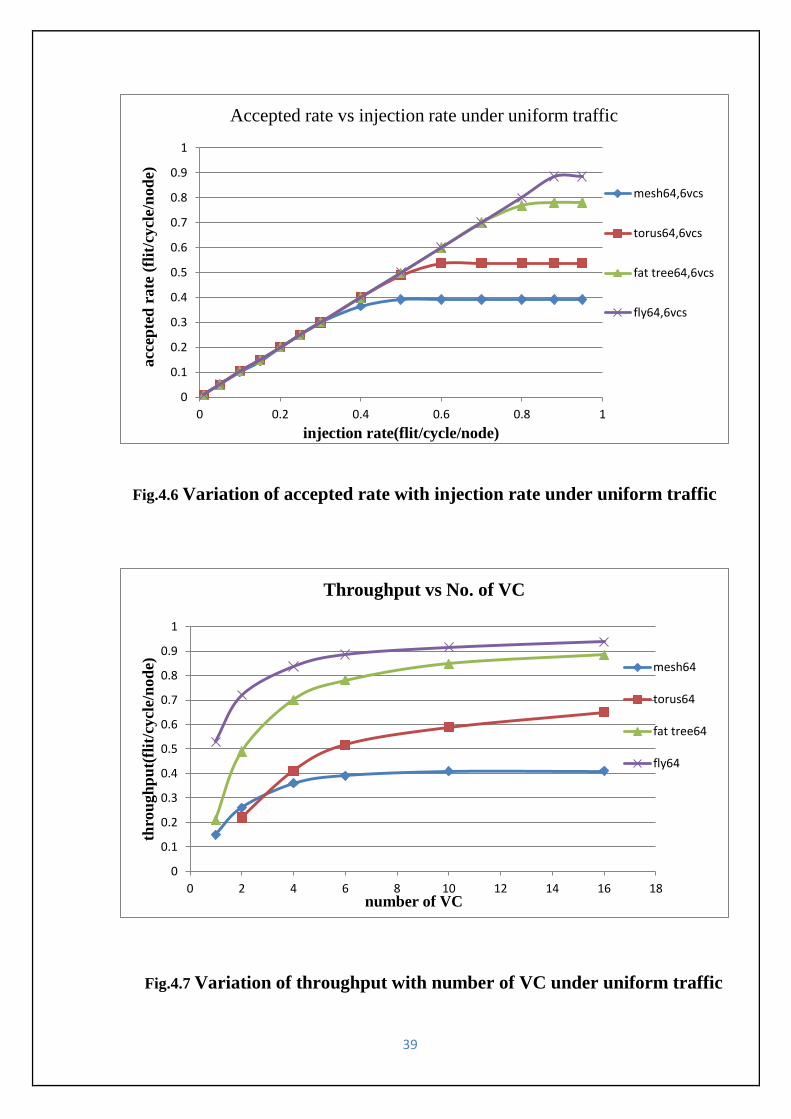
Fig.4.6 Variation of accepted rate with injection rate under uniform traffic------------------------39

Fig.4.7 Variation of throughput with number of VC under uniform traffic--------------------------39

Fig.4.8 (a) Variation of packet latency with injection rate under tornado traffic at VC 2--------40

Fig.4.8 (b) Variation of packet latency with injection rate under tornado traffic at VC 4--------40

Fig.4.8 (c) Variation of packet latency with injection rate under tornado traffic at VC 6---------41

Fig.4.9 Variation of accepted rate with injection rate under tornado traffic------------------------41

Fig.4.10 Variation of throughput with number of VC under tornado traffic-------------------------42

Fig.4.11 (a) Variation of packet latency with injection rate under neighbour traffic at VC 2----42

Fig.4.11 (b) Variation of packet latency with injection rate under neighbour traffic at VC 4----43

Fig.4.11 (c) Variation of packet latency with injection rate under neighbour traffic at VC 6----43

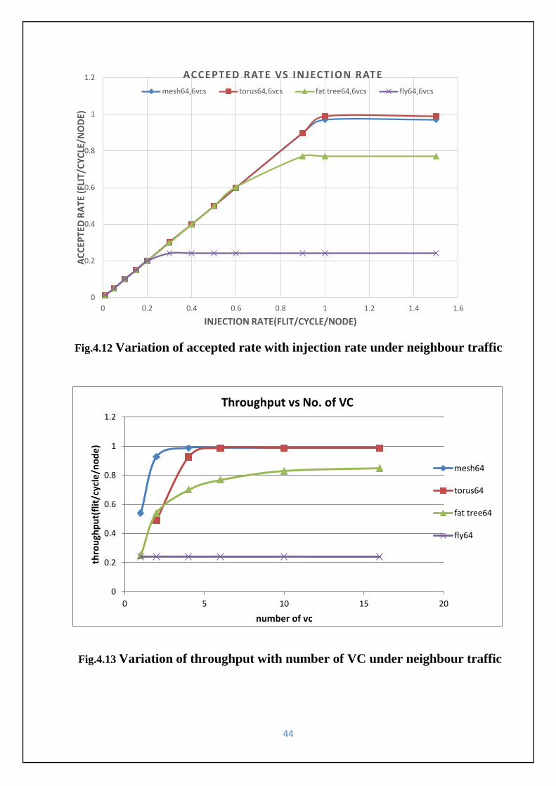
Fig.4.12 Variation of accepted rate with injection rate under neighbour traffic-------------------44

Fig.4.13 Variation of throughput with number of VC under neighbour traffic----------------------44

Fig.4.14 (a) Variation of packet latency with injection rate under bit compl.Traffic at VC 2----45

Fig.4.14 (b) Variation of packet latency with injection rate under bit compl.Traffic at VC 4----45

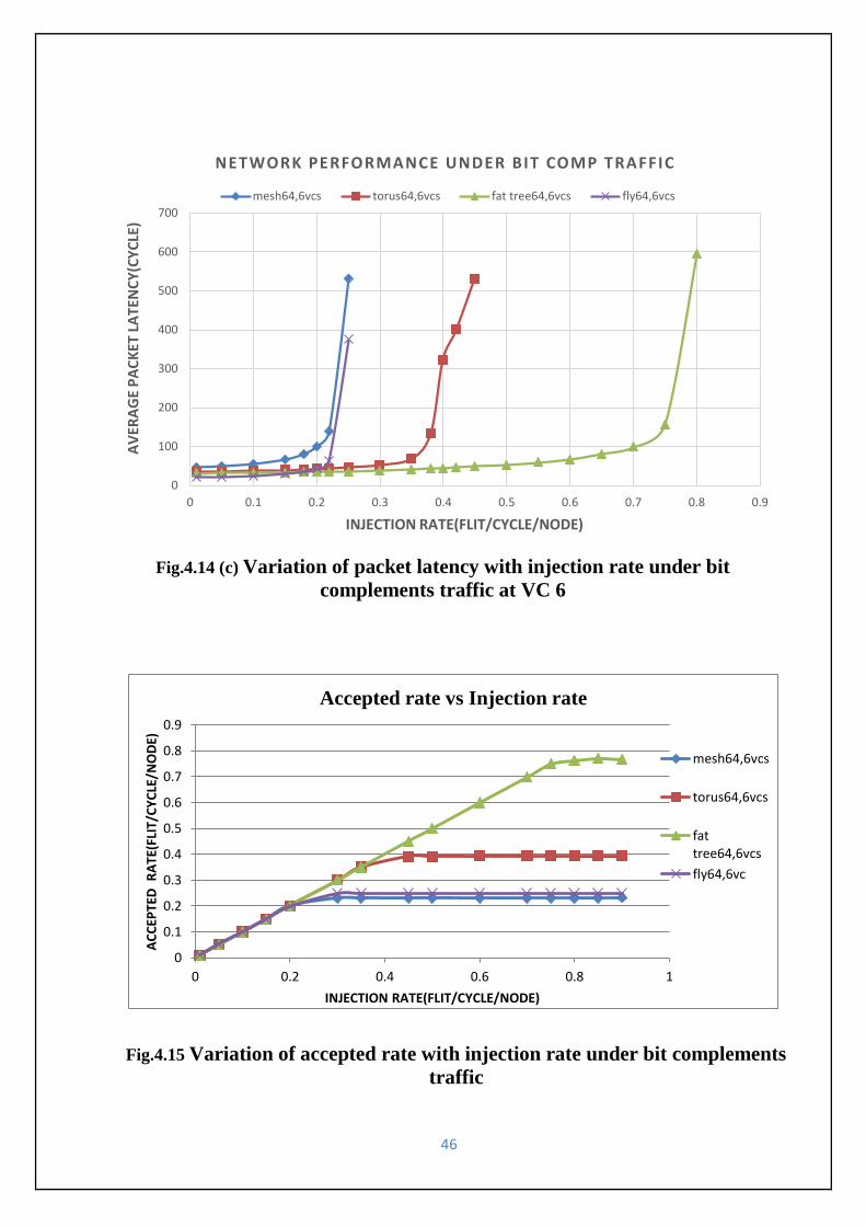
Fig.4.14 (c) Variation of packet latency with injection rate under bit compl. Traffic at VC 6----46

Fig.4.15 Variation of accepted rate with injection rate under bit complements traffic----------46

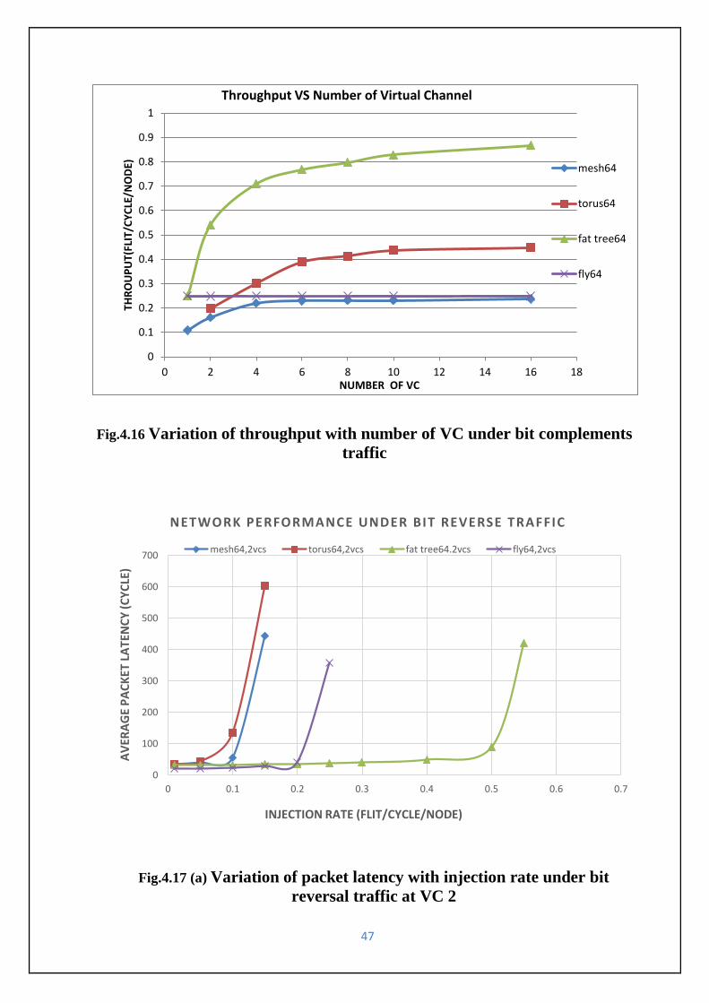
Fig.4.16 Variation of throughput with number of VC under bit complements traffic-------------47

Fig.4.17 (a) Variation of packet latency with injection rate under bit reversal traffic at VC 2--47

Fig.4.17 (b) Variation of packet latency with injection rate under bit reversal traffic at VC 4--48

Fig.4.17 (b) Variation of packet latency with injection rate under bit reversal traffic at VC 6--48

viii

Fig.4.18 Variation of accepted rate with injection rate under bit reversal traffic------------------49

Fig.4.19 Variation of throughput with number of VC under bit reversal traffic--------------------49

Fig.6.1 total power at different buffer depth of mesh interconnect network at VC2-------------63

Fig.6.2 total power at different buffer depth of mesh interconnect network at VC4-------------64

Fig.6.3 Total power at different buffer depth of torus interconnect network at VC2------------ 64

Fig.6.4 Total power at different buffer depth of torus interconnect network at VC4------------ 65

Fig.6.5 Total power at different buffer depth of Fat tree interconnect network at VC2---------65



Fig.6.8 Total power at different buffer depth of butter fly interconnect network at VC2-------67

Fig.6.9 Total power at different buffer depth of butter fly interconnect network at VC4-------67

Fig.6.10 Area compression of different interconnect network at VC2--------------------------------68

Fig.6.11 Area compression of different interconnect network at VC4--------------------------------68

Fig.6.12 Total power varying with buffer depth of different interconnect network--------------69

Fig.6.13 Area varying with buffer depth of mesh interconnect network-----------------------------69

Fig.6.14 Area varying with buffer depth of torus interconnect network ----------------------------70

Fig.6.15 Area varying with buffer depth of Fat tree interconnect network--------------------------70

Fig.6.16 Area varying with buffer depth of Fat tree interconnect network -------------------------71

ix

List of Tables

Table 4.1 Saturation throughput at different number of VC for different traffic------------------50

Table 5.1 Synthesis results of different interconnect network on FPGA with Flit Data Width of

8 bits---------------------------------------------------------------------------------------------------------56


16-------------------------------------------------------------------------------------------------------------56


32 ------------------------------------------------------------------------------------------------------------57

Table 5.4 Path delay of different interconnect network with Flit Data Width of 8 bits----------57

Table 5.5 Path delay of different interconnect network with Flit Data Width of 16 bits---------58

Table 5.6 Path delay of different interconnect network with Flit Data Width of 32 bits---------58

x

ABBREVIATIONS

SoC System-on-Chip

NoC Network-on-Chip

BFT Butterfly Fat Tree

VHDL VHSIC Hardware Description Language

VHSIC Very High Speed Integrated Circuit

FPGA Field Programmable Gate Array

DSP Digital Signal Processing

ASIC Application Specific Integrated Circuit

IP Intellectual Property

PDA Personal Digital Assistant

CBR Constant Bit Rate

LUT Look Up Table

IOB Input/output Block

GCLK Global Clock

FDW Flit data Width

FBD Flit Buffer depth

VC virtual channel

MPSoC Multiprocessor System on Chip

DOR Dimension order routing

1

\

Chapter one

Introduction

2

The advancement in technology, requirement of high performance computation–intensive

applications such as mobile and multi-processor application, enable the integration of many

resources such as CPU, DSP, Intellectual Property (IP) Cores and peripherals etc. into a single

chip, termed as multiprocessor System on Chip (MPSoC). The communication between these

cores is done efficiently which will enhance the requirement of scalability, higher bandwidth,

and better modularity along with increase in performance of the system to meet the required

computational task [1].

Network-on-Chip (NoC) has emerged as communication paradigm in many cores on chip

network and replacing traditional buses and crossbar network [2]. The basic building blocks of

NoC are routers, cores and network interface. NoCs consists of various nodes and links. Router

at every node is connected to the neighbour node via on-chip local wiring called interconnect

(links) that allows multiplexing of multiple communication between cores over this

interconnect to provide higher bandwidth and better scalability.so interconnect network

architecture for NoC is important recherché area for high performance and low area and power

consumption of NoC

1.1 Evolution of NoC interconnects: In the history of SoC interconnect network, the semiconductor industry looking at the

advancement of the system from a communication perspective that links chip’s individual

components amongst one another within the chip. The history of on-chip interconnect network

has three phases which describe in [3].

1.1.1 Shared bus interconnects:

Initially in MPSoC shared bus system is used for communication between processor and

memory and other devices. In this interconnect all core are connect by single link called as a

bus. In this system when a source uses the bus for communication to other source, other sources

cannot use that bus and have to wait for their turn.so arbiter become essentially for accessing

the bus efficiently by the sources. Due to this latency of system increases and performance of

system demean. Bus based system unable to meet bandwidth requirement with large no. of

nodes. Fig1.1 show conventional bus interconnects.

3

Figure 1.1 conventional bus interconnect

Figure 1.2 point to point interconnect

1.1.2 Point to Point interconnect: Previously designer use point to point interconnects for transfer of data inside network on

chip. IN this network cores are connected to other core straight by a link and communicate.

This system does not need arbiter. Network on chip with huge number of IP cores, needs

enormous routing area, large latency and large number of input and output pin for each core

and becomes very composite for connection point of view. Fig.1.2 show point to point

interconnect network.

4

Figure 1.3 3x3 mesh NoC

1.1.3 Network on Chip: As SoCs get larger number of IP cores, shared bus system and crossbar system were fail to

performed communication in side SoC. Shared bus network led to resource contention and

hierarchical bus architectures and crossbar designs generated complexity. Interconnection

networks offer an alternate solution to this communication paradigm and are becoming

persistent in SoC. A NoC based interconnect network is a well-organized and efficiently use of

limited communication channel while maintaining low packet latency, high saturation

throughput, high communication bandwidth amongst different IPs core with a minimum area

and low power-dissipation. As system density and integration of many cores continue

increasing, many designers discovered that it is more efficient to route packets, not wires [4].

Using an interconnection network in a SoC permits limited bandwidth to be shared between

cores so that it can be used efficiently. Interconnect network efficiently use of communication

resources, making SoCs easier to design, less complex, and optimized. Fig. 1.3 shows a 3×3

Mesh interconnect network for NoC.

5

1.2 Literature review: Network on Chip are emerging as an important paradigm for system on chip (SoC). SoC

platform consist large no. of processor according to publication [5], [6], [7].

NoC has many recherché area interconnect network is one of them. As the number of node

increases then complexity of NoC increases so we required efficient interconnect network

which is scalable and flexible.

Ju and Yang [8] analysis three topologies (mesh, torus and hierarchical mesh) and final

simulate 2x4 2D-torus topology and design single routing node architecture on FPGA. S.kunda

et al. [9] design and evolution of tree base mesh NoC using virtual channel router and

compared with butterfly and fat tree. M.S. Abdelfattah at el [10] presented detail design trade-

off for hard and soft FPGA based NoC. J. Lee and L. Shannon [11] describe effect of node size

of NoC on FPGA.

Jason lee et al [12] presents the prediction on performance analysis of ASIC NoCs

implementation in FPGA and investigates different topologies to find out appropriate

topologies for ASIC.

Abba and lee [13] presented a Bayesian network approach and self-adaptive scheme for NoC

parameter based performance analysis on FPFA based NoC.

M.K. Papa Michael [14] present a tool CONNECTS for design of NoC in FPGA. N.Jiang et al

[15] present C+ based cycle accurate simulator for NoC who support many topologies and

traffic pattern. G. Schelle et al [16] present on chip interconnect architecture exploration on

FPGA.

P.P. Pande et al [17] done performance evolutions of three topologies mesh torus and spin in

term of latency throughput and energy. S. abba et al. [18] present a Parameter based approach

for performance evaluation and design tradeoff for inter connect architecture using FPGA for

network on chip.

6

1.3 Motivation: Now a days chip manufacturers are annoying to release the multiprocessor products with

numerous cores in the single system. Initial bus and crossbar system are used for

interconnection of multicore processor. So bus based and crossbar system failed to provide an

efficient communication system because Bus-based architectures have trouble scaling with

increasing number of IP blocks and decreasing geometries. So Network-on-Chip derived into

presence and exchanges bus based and point-to-point systems. Network-on-chip is the latest

paradigm in interconnect technology which has several advantages. It has been an active area

for research for over a decade and still many new NoC concepts are being developed on a

regular basis. NoCs offer superior performance, power and area trade-offs as the number of

modules increases and NoC performance and area on chip manly depend upon interconnect

architecture which is used in NoC

1.4 Thesis objective: Study of Network on Chip basics.

Study of different interconnect network.

Study of different NoC parameters.

Performance analysis of different interconnect network.

Study the effect of different NoC parameter on FPGA resource of interconnect

network.

Power and area analysis of different interconnect network.

1.5 Thesis plan:

The approach of thesis is to describe the different interconnect network for NoC and

performance analysis. This thesis is plan as:

Chapter 2 discuss about different recherché area of network on chip and building block of NoC.

Chapter 3 discuss about classification of interconnect network architecture for NoC and

performance matrix for interconnect network.

Chapter 4 Discuss about the performance analysis of different interconnect network under

different traffic pattern.

7

Chapter 5 Discuss about effect of NoC parameter on interconnect network on FPGA resources

and critical path delay.

Chapter 6 Discuss about Powers and area analysis of different interconnect network at 65 nm

technology.

Chapter 7 Discuss about the conclusion and future works in interconnect network.

8

Chapter Two

Network on Chip: A new SoC paradigm

9

Figure 2.1 Mesh topology Figure 2.2 Torus topology

Network on chip (NoC) is an on-chip communication system between different intellectual

property IP cores. NoC consider most suitable option in place of bus and crossbar based

interconnection architecture in core based system on chip (SoC) design .In the design IP cores

are connected to each other through a router.

NoC paradigm can be classified into four research areas.

2.1 Communication infrastructure paradigm:

2.1.1 Topologies:

Network topologies provide different path over which packet travel from Source to

destination. It refers as a static arrangement of router or node and channel .it plays important

role in NoC performance. Topologies selection for NoC design depends upon the basis of its

cost and performance. Topologies can be regular and irregular. Fig2. (1-5) show some

topologies among this Figure 2.1 mesh topology with 9 core, this is a regular type of topology

and simplest among all topologies. Figure.2.2 torus topology with 9 cores, this is similar to

mesh with wrap around link. Figure 2.3 three stage fat tree topology with 8 cores, this is

irregular topologies. Figure 2.4 show butterfly topologies with 4 inputs 4 outputs and 3 router

stages. Figure 2.5 star topology this look like a star .which consist one router at centre of

topology and all other router connect to the centre router by a proper link.

10

Figure 2.3 Fat Tree topology Figure 2.4 Butterfly topology

Figure 2.5 Star topology

Figure 2.6 classical router architecture

2.1.2Router: Router is the most pivotal module for design of communication infrastructure inside NoC.

Latency, Throughput meet and Tight Area and power constrain of network depends upon router

architecture design. The main functionality of router is route the packet from source to

11

Figure 2.7 virtual channel router with five pipeline stage

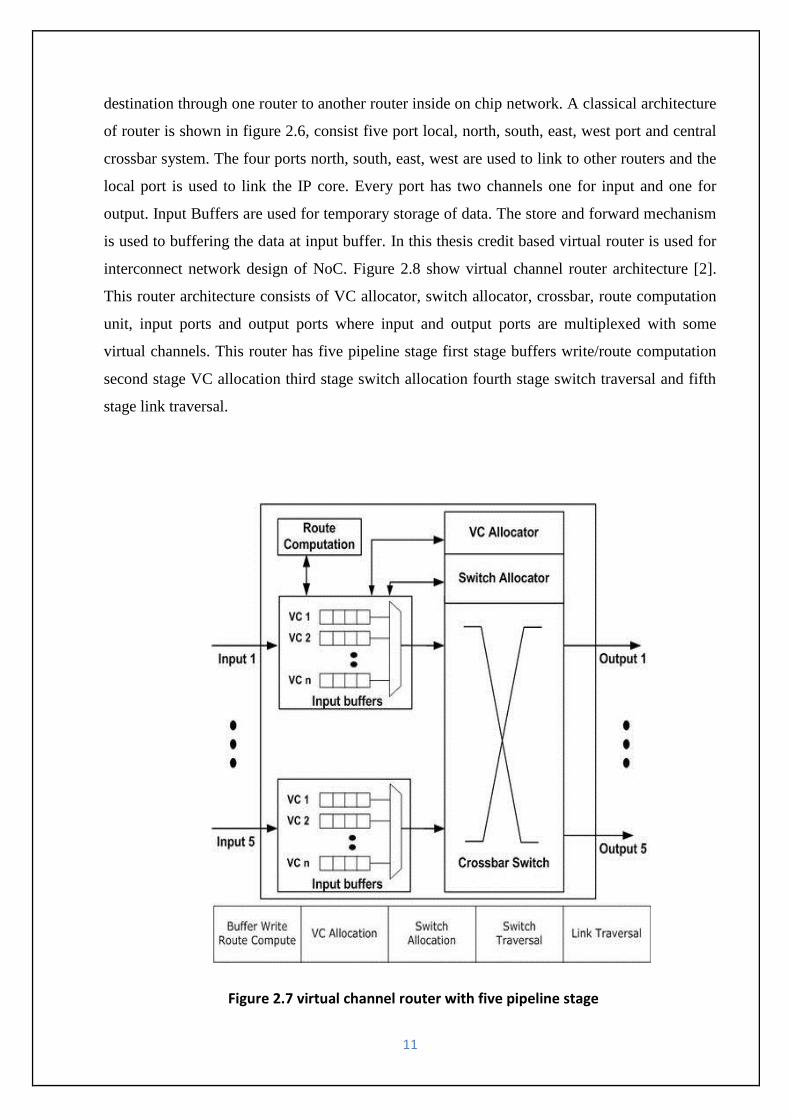
destination through one router to another router inside on chip network. A classical architecture

of router is shown in figure 2.6, consist five port local, north, south, east, west port and central

crossbar system. The four ports north, south, east, west are used to link to other routers and the

local port is used to link the IP core. Every port has two channels one for input and one for

output. Input Buffers are used for temporary storage of data. The store and forward mechanism

is used to buffering the data at input buffer. In this thesis credit based virtual router is used for

interconnect network design of NoC. Figure 2.8 show virtual channel router architecture [2].

This router architecture consists of VC allocator, switch allocator, crossbar, route computation

unit, input ports and output ports where input and output ports are multiplexed with some

virtual channels. This router has five pipeline stage first stage buffers write/route computation

second stage VC allocation third stage switch allocation fourth stage switch traversal and fifth

stage link traversal.

12

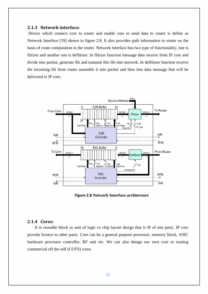
Figure 2.8 Network Interface architecture

2.1.3 Network interface: Device which connect core to router and enable core to send data to router is define as

Network Interface [19] shown in figure 2.8. It also provides path information to router on the

basis of route computation in the router. Network interface has two type of functionality, one is

flitizer and another one is deflitizer. In flitizer function message data receive from IP core and

divide into packet, generate flit and transmit this flit into network. In deflitizer function receive

the incoming flit from router assemble it into packet and then into data message that will be

delivered to IP core.

2.1.4 Cores: It is reusable block or unit of logic or chip layout design that is IP of one party. IP core

provide licence to other party. Core can be a general purpose processor, memory block, ASIC

hardware processor controller, RF unit etc. We can also design our own core or reusing

commercial off the self (COTS) cores.

13

2.1.5 Channels:

Wire which is used to interconnect the router to form network is define as a channel. They

are characterizing by their width and length. The width of channel is defined by size of flit

which is use for transmission of data. The channel length is defined by the distance between

two routers. The delay of flit is depending upon the channel length.

2.2 Communication paradigms:

2.2.1 Routing algorithm:

Routing algorithm plays an important role for efficient communication inside on chip

network between different nodes. First we decide topology for network on chip and then chose

an explicit routing algorithm. Routing algorithm finds out all possible paths for transmission of

packet from source to destination and route the packet through one path. It also distributes the

traffic uniformly throughout network so it will avoid hotspot and minimizing contention at one

node and improve latency and throughput of network. The design complexity of router depends

upon routing algorithm so it also affects area and power of network. Routing algorithms are

classified into three types.

1) Deterministic, 2) oblivious, 3) adaptive.

Deterministic routing determines the path between source and destination determine in

advance by source node. Dimension order routing (DOR) is one of the example of deterministic

routing in this routing packets traverse network through dimension by dimension. It is simplest

routing algorithm among all. Fig.2.9 show XY dimension-order routing who first send the

packet in X direction and then in Y direction.

Oblivious routing algorithm determines all in all possible paths between source node and

destination node and message traverse through path without bother about congestion in

network. Fig.2.9 shows oblivious routing in this message can be randomly send either X-Y

route or Y-X route.

There are many paths between sources to destination. In adaptive routing selection of the path

depend upon dynamic condition of network. Fig.2.9 show adaptive routing in this message take

north direction at (1, 0) router instead of east direction due to congestion.

Routing can also be classified into minimal and non-minimal routing algorithm. Routing

schemes which uses direct possible path for communication is known as minimal routing and

apposite of this called non minimal routing. Advantage of non-minimal over minimal routing

14

Figure 2.9 Example of DOR Adaptive and oblivious routing

including possibility of bleaching network load and fault tolerance. Various properties of the

interconnection network are a straight significance of the routing algorithm used. Amongst

these properties we can quote the following routing:

Connectivity: Capability to route packets from any source node to any destination node.

Adaptively: Capacity to route packets through alternate paths in the presence of contention or

faulty mechanisms.

Deadlock and livelock freedom: Ability to assurance that packets will not chunk or, stroll

across the network continually.

2.2.2 Switching techniques:

Switching techniques [20] also called flow control mechanism of message inside the

network. Switching is a technique by which data move from input channel to output channel of

router. Latency of network mainly depends upon switching technique. They are classified into

two type 1) circuit switching 2) packet switching .packet switching further classified into a)

Store and forward b) Virtual cut through c) Wormhole switching. In this thesis wormhole

switching is used for analysis of all interconnect network. In circuit switching [20] complete

15

Figure 2.10 Store and Forward Example

message is transmitted from one router to another router until message reaches their

destination.it is message based flow control mechanism. In packet switching message divide

into packet and then transmitted from input channel to output channel. They are classified into

flowing

2.2.2.1 Store and forward:

In store and forward switching a complete packet moves from one router to next router.

In this switching packet can only forward to next router when it complete receive.fig.2.10

shows store and forward switching techniques in which router 0 send a packet to router 8 this

complete process take 24 clock cycle. In this switching packet divide into flits, head flit

payload flit, tail flit. In this switching router first receive head flit and then payload flits and tail

flit show ending of packet. Now next head flit of new packet receive at router.

2.2.2.2 Wormhole:

Wormhole switching technique [20] split packet into flits (head flit, body flit and tail

flit). Head flit caries control and routing of packet, body load flits contain data, tail flit contain

information of ending of packet. Fig.2.11 shows wormhole switching with 2 flit buffer size

with contention at router2.it require only 11 clock cycle for transmission of packet from router

0 to router 8. Wormhole switching sends a flit in pipelining fashion due to this latency of

network decrease so it is most suitable and preferable switching techniques for implementation

of NoC.

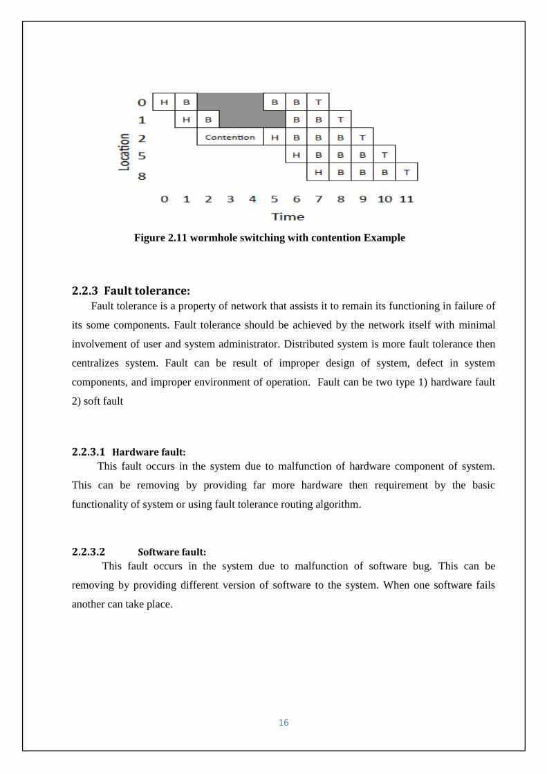
16

Figure 2.11 wormhole switching with contention Example

2.2.3 Fault tolerance: Fault tolerance is a property of network that assists it to remain its functioning in failure of

its some components. Fault tolerance should be achieved by the network itself with minimal

involvement of user and system administrator. Distributed system is more fault tolerance then

centralizes system. Fault can be result of improper design of system, defect in system

components, and improper environment of operation. Fault can be two type 1) hardware fault

2) soft fault

2.2.3.1 Hardware fault:

This fault occurs in the system due to malfunction of hardware component of system.

This can be removing by providing far more hardware then requirement by the basic

functionality of system or using fault tolerance routing algorithm.

2.2.3.2 Software fault:

This fault occurs in the system due to malfunction of software bug. This can be

removing by providing different version of software to the system. When one software fails

another can take place.

17

2.2.4 Reliability: The system and its component ability to achieve its mandatory functions under stated

conditions for a specified period of time is define as a reliability of system. Reliability deal

with the life cycle and risk of failure of system.it also related to safety of system.

2.3 Evolution framework: It is one of important research area of NoC to efficiently and errorless analysis of different

NoC to have a good understanding of attainable throughput, latency, and bandwidth of the

network. Evolution framework defines a communication API for performing design

exploration, network level performance modelling of NoC components at various levels of

abstraction. It is of two types

2.3.1 Software evolution framework: This evolution framework based on system C/C++. Cycle accurate simulator is a software

type of simulator and simulation time increases as we move toward high accuracy and a precise

simulation. Jiang et al. develop C++ based booksim simulator [21]. Booksim support mesh,

torus, fat tree, butterfly and cmesh topologies and only simulator who support virtual channel

router with synthetic traffic. Jain et al develop NIRGAM system C based simulator [22].

NoCTweak is developed by Anh T. Tran et al who support both synthetic traffic and embedded

application pattern.

2.3.2 FPGA based evolution framework: In recent years, FPGA based emulation framework have come into existence since they

overcome the limitations imposed by the software simulators and allow for faster architectural

space explorations and detailed, accurate design . Genko et al develop a HW/SW evolution

platform based on FPGA with an embedded PowerPC processor and emulating a network of six

routers.

2.4 Application mapping: Application mapping is also an important area of NoC research.it is technique by which map

core to router. Application mapping [23] can be divided into two types.

2.4.1 Dynamic mapping: Dynamic mapping is a mapping of tasks online during running time. The tasks are mapped

on NoC on the basis of current status of NoC it can be changed during execution of application.

18

Dynamic mapping always sense block condition and remove this condition by distribute the

load among processors.

2.4.2 Static mapping: Static mapping is an off line mapping strategy.it mapped task before application run on

NoC. Static mapping permanently define greatest placement of task before run. For NoC static

mapping is used.

19

Chapter three

Interconnect network architecture

20

Figure 3.1 Example of interconnect network

Interconnect networks are presently being used for many applications, ranging from small

mobile system to wide area computer networks. Interconnect network play significant role in

performance of multicomputer networks. Interconnect network is a programmable system that

transfer data between terminals. Fig.3.1 an example of interconnect network [1]. Six terminals

labelled T1 to T6 are connected interconnect network by bidirectional channel. When terminal

T3 wishes to communicate with terminal T5, it sends a message into the network and the

network delivers the message to T5. The network is a system because it is contain: buffers,

channels, switches, and controls that work together to deliver data from one terminal to another

terminal.

Interconnect network can be categorised according to process method (synchronous or

asynchronous) and control unit. Interconnect network can be categorized into four classes

which is shown in Fig.3.2. This figure shows hierarchy [24] of subclass.

21

Figure 3.2 taxonomy of interconnect network

22

Figure 3.3 Single bus shared medium network

3.1 Shared medium network: It is minimum complex interconnect network among all .it share a single transmission

medium to all communication terminal. In this network only single device is allowed to

transmit data in the network at an interval due to this latency is high of this network. It is

passive type of network because network itself does not able to generate message. Device

which is connected to network has requester driver, receiver circuit to handle the transmission

of message data and address. Shared medium network is used arbitration strategy to resolve

network access conflict. It has ability of atomic broadcasting in which all devices on the

network can monitor network activity and access the information on the shared medium

network. This ability make network to support various application of one to all and one to

many communication services. Due to bandwidth limitation shared medium network only

support restricted number of devices before medium become a bottleneck. Limited bandwidth

restricted Shared medium network use in multiprocessor network. It is divided into two major

classes: local area network basically uses to build a computer network for transmission of data

in few kilometre distance.it is subdivided into contention bus, token bus, and token ring.

Backplane bus is used for internal communication in uniprocessor and multiprocessor network

fig 3.3 show single bus network [24] in which memory and processor are connected by single

bus.

23

Figure 3.4 A generic node architecture

3.2 Direct network: Shared medium network is bus based system which is not scalable because network is

bottleneck when processor increases in the network. So direct network use to resolve scalability

problem. The direct network is a common network that balances large no. of processor in a

single network. In this network nodes are directly connected to subset of other nodes by

bidirectional channel. Every node is a programmable computer with its own processor, memory

and other secondary devices. Fig 3.4 shows a generic node [1] which contains processor,

memory and router. Router manages communication among all nodes. Due to this reason direct

networks are also called as router based network. Every router has some no. of input and output

ports. Internal channels or ports are used for connect local processor and memory to router.

Outer channels are used for communication between routers. More internal channels are used

for avoiding bottleneck in the network. Every node has restricted number of input and output

channel and each input channel associate with one output channel. In this network each node is

connect directly.

Direct network have been traditional model by Graph G (N, C) where vertices N represent

number of node in the network and edge C represent set of channel. Direct network can be

classified by three factor topology, routing, switching. On topologies basis It is sub divide into

following.

24

Figure 3.5 (a) 2-ary 4-cube (b) 3-ary 2-cube torus (c) 3-ary 3-D mesh

Figure 3.6 Tree topology (a) no uniform binary tree (b) uniform binary tree

3.2.1 Strictly orthogonal topology: Strictly orthogonal topology [24] is less complex topology and also requires very simple

routing. Thus, routing algorithm can be easily and efficiently realized in hardware. In this

topology each node is define by coordinates in the n-dimension space. This is sub divided into

1) n-dimension mesh 2) k-ary n-cube 3) torus 4) hypercube fig 3.5 shows all strictly orthogonal

topology.

3.2.2 Other direct network topology: Tree topology is also a direct network topology. This topology has one root node linked to

certain number of branch nodes or leaf node. Tree topology has characteristic that root node has

single parent node. Fig.3.6 show tree topology which is divide into (a) unbalanced binary tree

b) balance binary tree

25

Figure 3.7 an N x M Crossbar network

3.3 Indirect network: Indirect network also called switch based network and also important class of interconnect

network. In this network two nodes are communicate indirectly through the switch. Every node

has a network interface that connects to a network switch. This switch has some port to connect

nodes. Each port has input and output link. These ports are connected to processor and memory

element to the switch and remaining ports are connected to the port of other switch. Indirect

network can also be characterized by Graph G (N, C) where N is set of switch, C is set of

unidirectional and bidirectional link between the switch. Indirect network classified into two

types

3.3.1 Crossbar network:

This network connects the nodes through single N x N switch network. This switch

network is known as crossbar network and connection of node through this switch is called

crossbar network. Crossbar network is much cheaper than direct network.Fig.3.7 crossbar

network with N input port and M output port through which processor and memory are

connected and various processors can communicate simultaneously without contention.

Crossbar network have been used in small scale shared memory multiprocessor where all

processors are permitted to access memory at once. When two processors resist for same

memory module, then arbiter select one processor and this processor proceed and while other is

wait until first processor free them. The cost of crossbar network is O (N M) which is rises with

increment in N and M.

26

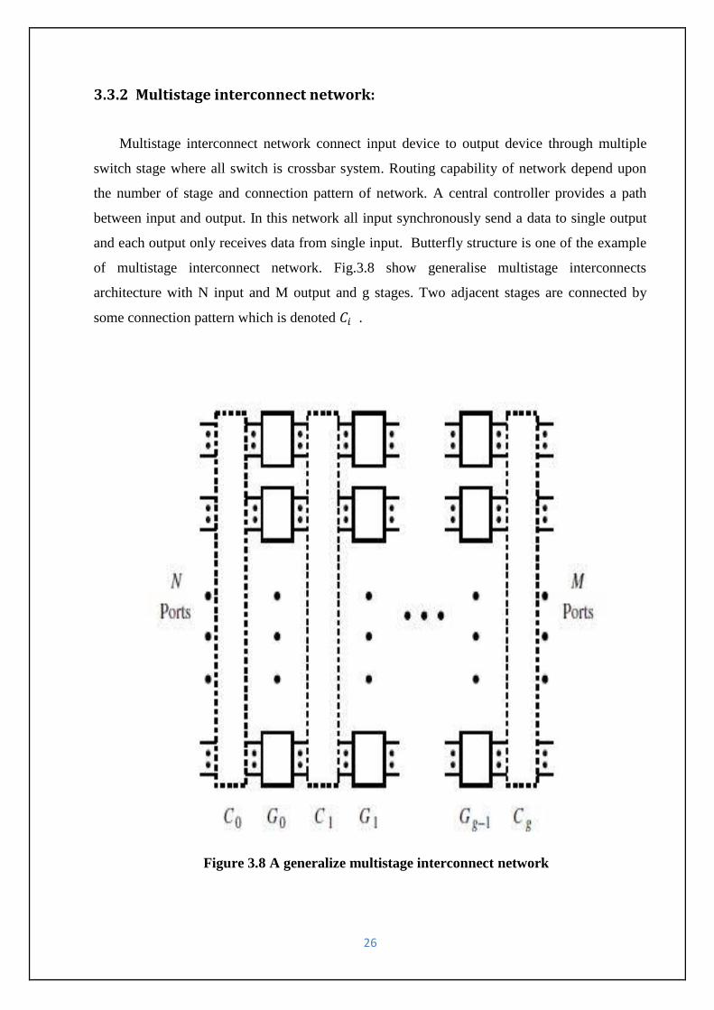
Figure 3.8 A generalize multistage interconnect network

3.3.2 Multistage interconnect network:

Multistage interconnect network connect input device to output device through multiple

switch stage where all switch is crossbar system. Routing capability of network depend upon

the number of stage and connection pattern of network. A central controller provides a path

between input and output. In this network all input synchronously send a data to single output

and each output only receives data from single input. Butterfly structure is one of the example

of multistage interconnect network. Fig.3.8 show generalise multistage interconnects

architecture with N input and M output and g stages. Two adjacent stages are connected by

some connection pattern which is denoted .

27

3.4 Performance matrix for interconnect architecture: Performance matrix [25] that ever interconnect architecture must satisfied

Small latency

High throughput

Low power consumption

Area

Scalability and reliability

But there are some important parameter for analysis of interconnect network for NoC latency,

throughput, total power dissipation, area requirement.

3.4.1 Latency:

Latency is defined by the time interval in clock cycles between header flit injected into the

network at the source node and the arrival of a tail flit at the destination node. Total packet

latency is combination of head latency and serialization latency.

Where is total packet latency, head flit latency, serialization latency

The serialization latency is the time required for the tail to catch up the time that is the time for

a packet of length L to cross a channel with bandwidth B.

The head latency is the time required for the head flit of the message to cross the network, In

the absence of contention, head latency is the sum of two factors determined by the topology:

router delay and time of flight,

Average hop count, is single router delay

28

Average distance between sources to destination, propagation velocity of packet

Then average packet latency is

3.4.2 Throughput: Throughput is defined as the total number of packet arrived per IP at the destination core in

a single clock cycle.

Throughput T, can be define as following.

Where Total arrived Packets means the no. of data packets that have reached their destination

terminal

Data Packet Length can be measured in bits or flits,

No. of IP Cores is the number of active IPs that are participating in the traffic scenario,

Total Active time is the total time measured from the incidence of the first packet inception to

the last packet reception.

Thus, throughput gives a measure of the active part of the maximum load that the network can

handle.

29

Figure 3.9 A module hierarchy of booksim

3.5 Simulator used: booksim Booksim [21] is interconnected network simulator. This simulator is designed as companions

of textbook by dally and towels [1]. Booksim is cycle accurate and high level flexible

simulator for network on chip. Booksim provide modelling of all NoC components. The

simulator itself is written in C++ and has been specifically tested with the GNU G++ compiler.

The front end of the simulator uses LEX and YACC generated parser to process the simulator

configuration file; however, unless you plan on making changes to the front end parser, LEX

and YACC are not needed. Booksim support following type of traffic

uniform traffic

bit-reversed traffic

bit-complement traffic

tornado traffic

neighbour traffic

Fig. 3.9 show module hierarchy of simulator

30

Chapter four

Performance analysis of different

Interconnect network

31

In this chapter we analysis some common available interconnect network and trade-off between

this interconnect network on the basis of latency and throughput and saturation throughput.

Different parameter are used for analysis of interconnect network. We analysis interconnect

network with higher nodes. Topology was designed using CONNECT: A Tool for NoC

generation [14]

4.1 2D Mesh:

2D Mesh interconnect is a very widely held network in Network on Chip due to its

simplified implementation, simplicity of the XY routing algorithm and the network scalability

Fig. 4.1 shows 8x8 2Dimensional Mesh interconnect network. Mesh interconnect network

contains m router in X dimension and n router in Y dimension. The routers are located at each

connection point of two links and cores positioned nearby the routers. Mesh interconnect

network is a unique network interconnect architectures of NoC in this nodes are linked through

many routers. Mesh interconnect network is best choice for interconnect network because it

similarly as die structure. Nodes in the Mesh are linked to other node by XY-dimension pattern,

as shown in Fig.4.1. The intellectual property (IPs) cores are coupled to a NoC router via a

Network Interface (NI). Mesh network is generally used in parallel computer architecture

platforms [24] due to simple network architecture. Mesh interconnect network is a direct

network which provides a uniform interconnection between nodes. The design of router for

Mesh interconnect network requires more time to design and also complex structure. In mesh

interconnect network pipelined allowed at High frequency schemes, but pipeline prevention at

low traffic is necessary for possession little delay at the router. This is one of the main

disadvantages of the Mesh network. There will be fewer available of node at the corners of

mesh and edges of network, since these routers have a higher average distance from other

router [26]. 2D Mesh network has some other disadvantages such as long network diameter as

well as energy inefficiency because of the extra hop count.

32

4.1 2D Torus:

Fig.4.2 represents an m x n torus interconnect network (8x8 2D Torus) based on an m x n

mesh interconnect network with an extra link connection added to each row and column. This

extra link is called wraparound link. This link support to reduce the area of network and the

average hop distance between nodes. Every router is linked to four adjacent routers and one IP

core. Every router has five ports east, west, north, south and local port. Adding wraparound

links to the mesh creates the torus interconnect network who decrease the average hop counts

and increasing the bandwidth. These links also increase the no. of connecting channels per

node. A Torus interconnect network has better path diversity and extra minimal routes path

than a Mesh network [1]. There is one drawback of torus network is that large latency and

larger cost.

Fig.4.1 structure of 8 x 8 Mesh interconnect network

33

4.3 Fat-tree: Fat tree is binary tree based interconnect network in parallel computer architecture for

communication. In a Fat-tree interconnect network [27] nodes are routers and leaves are

resources. The routers above a leaf node are known as the leaf’s predecessor and the leaves

beneath a predecessor are known as children predecessor. Every node has pretend predecessor,

permitting huge quantity of additional routes between nodes. We designated the arrangements

of the Fat tree providing Fat tree interconnect network has an exceptional characteristic which

allows it to use full channel bandwidth by any node for communication with other node in the

network. fat tree has identical bandwidth at any bisection.

Fig.4.2 structure of 8 x 8 2D Torus network

34

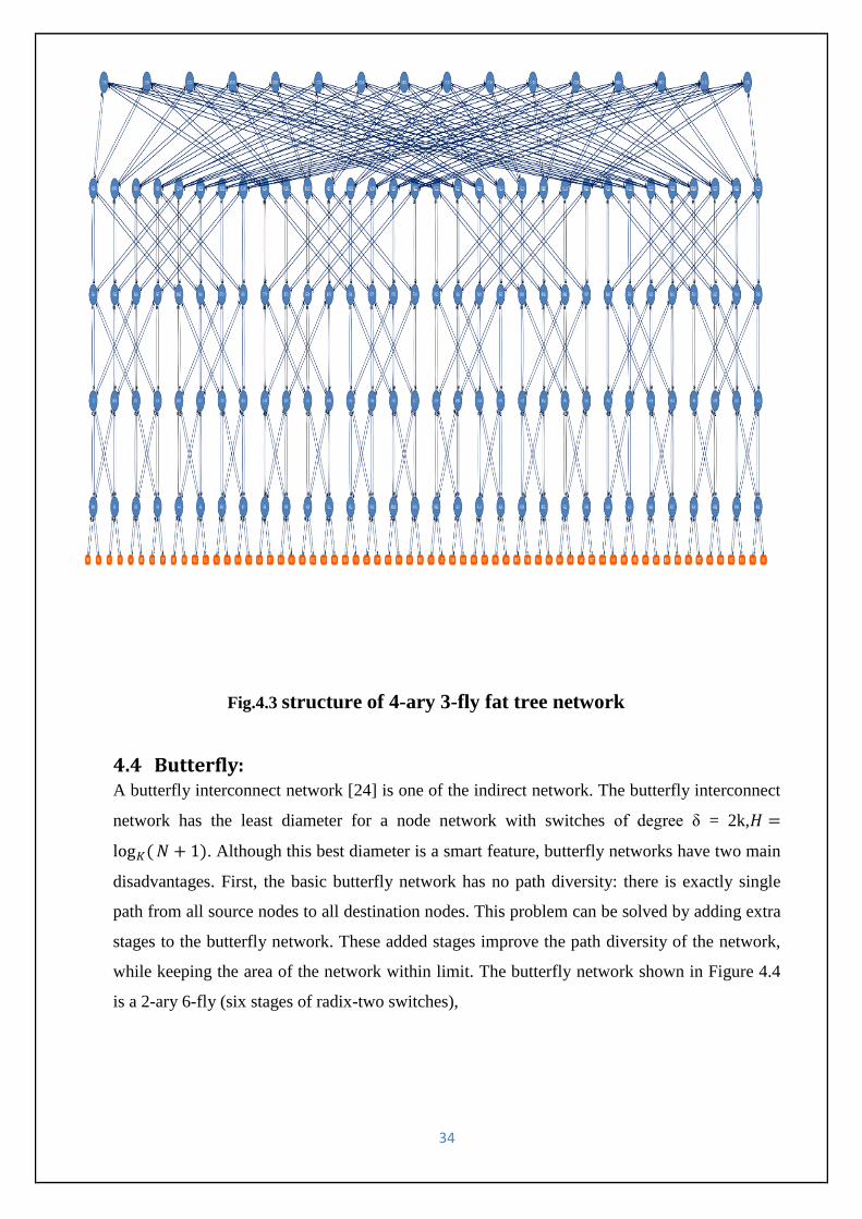
4.4 Butterfly: A butterfly interconnect network [24] is one of the indirect network. The butterfly interconnect

network has the least diameter for a node network with switches of degree δ = 2k,

. Although this best diameter is a smart feature, butterfly networks have two main

disadvantages. First, the basic butterfly network has no path diversity: there is exactly single

path from all source nodes to all destination nodes. This problem can be solved by adding extra

stages to the butterfly network. These added stages improve the path diversity of the network,

while keeping the area of the network within limit. The butterfly network shown in Figure 4.4

is a 2-ary 6-fly (six stages of radix-two switches),

Fig.4.3 structure of 4-ary 3-fly fat tree network

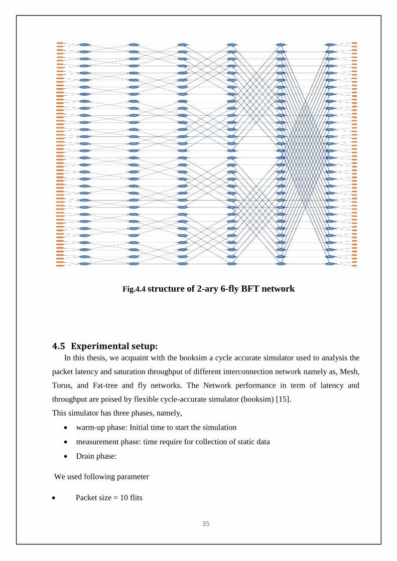
35

4.5 Experimental setup: In this thesis, we acquaint with the booksim a cycle accurate simulator used to analysis the

packet latency and saturation throughput of different interconnection network namely as, Mesh,

Torus, and Fat-tree and fly networks. The Network performance in term of latency and

throughput are poised by flexible cycle-accurate simulator (booksim) [15].

This simulator has three phases, namely,

warm-up phase: Initial time to start the simulation

measurement phase: time require for collection of static data

Drain phase:

We used following parameter

Packet size = 10 flits

Fig.4.4 structure of 2-ary 6-fly BFT network

36

Buffer Depth = 16bits

Injection process = Bernoulli

injection rate varied from .1 to 1

warmup_period =3

sample period=10000

Virtual channel allocator = islip

switch allocator = islip

The Routing algorithm: Dimension order routing (DOR) [28] for Mesh and Torus

networks and Nearest Common Ancestor (NCA) for Fat tree network dast-tag for fly

network.

4.6 Traffic pattern: In this thesis synthetic traffic pattern are used to analysis of different interconnect network.

4.6.1 Uniform traffic:

Uniform traffic, in which each source sends similar data to every destination, this is the

frequently used traffic pattern in interconnect network performance estimation. Uniform traffic

is very kind because it has a god load balancing .

4.6.2 Permutation traffic: In this traffic each source is sends all of its traffic to a single destination, it is classified in

two type.

4.6.2.1 Bit permutation:

Bit permutations are a subclass of permutations traffic in which the destination address is

calculated by permuting and selectively complementing the bits of the source address.

bit-reversed traffic

bit-complement traffic

37

0

100

200

300

400

500

600

0 0.1 0.2 0.3 0.4 0.5 0.6 0.7 0.8 0.9 1

AV

ERA

GE

PA

CK

ET L

ATE

NC

Y(C

YC

LE)

INJECTION RATE(FLIT/CYCLE/NODE)

N ET W O R K P ER F O R M A N C E U N D ER U N I F O R M T R A F I C P A T T ER N

mesh64 ,2vcs Torus64,2vcs Fat tree64,2vcs fly64,2vcs

4.6.2.2 Digit permutations:

In this traffic the digits of the destination address are determine from source address

digits. In this traffic the digits of the destination address are calculated from source address

digits. it is two type.

tornado traffic

neighbour traffic

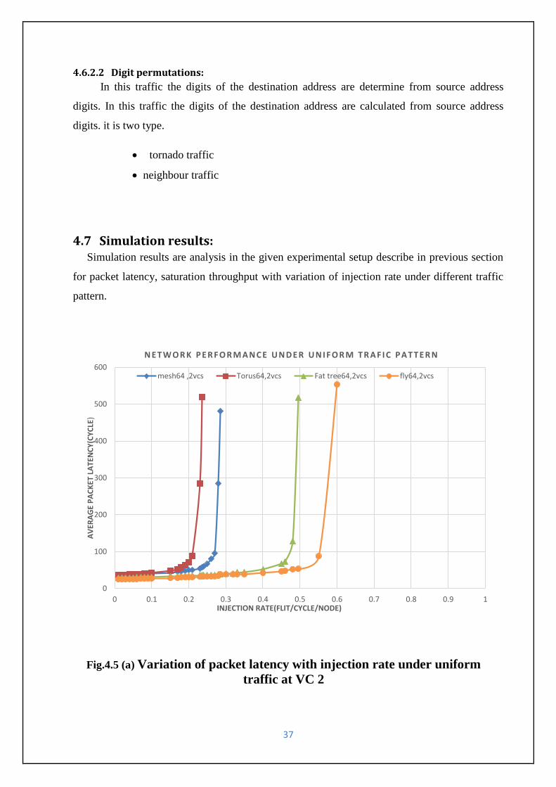
4.7 Simulation results: Simulation results are analysis in the given experimental setup describe in previous section

for packet latency, saturation throughput with variation of injection rate under different traffic

pattern.

Fig.4.5 (a) Variation of packet latency with injection rate under uniform

traffic at VC 2

38

0

100

200

300

400

500

600

0 0.1 0.2 0.3 0.4 0.5 0.6 0.7 0.8 0.9 1

AV

ER

AG

E P

AC

KE

T L

AT

EN

CY

(CY

CL

E)


N ET W O R K P ER F O R M A N C E U N D ER U N I F O R M T R A F F I C P A T T ER N

mesh64,4vcs torus64,4vcs fa tree64,4vcs fly64,4vcs

0

100

200

300

400

500

600

700

0 0.2 0.4 0.6 0.8 1

aver

age

pack

et l

ate

ncy

(cycl

e)

injection rate(flit/cycle/node)

Network performance under uniform traffic pattern

mesh64,6vcs torus64,6vcs fat tree64,6vcs fly64,6vcs

Fig.4.5 (c) Variation of packet latency with injection rate under uniform

traffic at VC 6

Fig.4.5 (b) Variation of packet latency with injection rate under uniform

traffic at VC 4

39

0

0.1

0.2

0.3

0.4

0.5

0.6

0.7

0.8

0.9

1

0 0.2 0.4 0.6 0.8 1

acc

epte

d r

ate

(fl

it/c

ycl

e/n

od

e)


Accepted rate vs injection rate under uniform traffic

mesh64,6vcs

torus64,6vcs

fat tree64,6vcs

fly64,6vcs

0

0.1

0.2

0.3

0.4

0.5

0.6

0.7

0.8

0.9

1

0 2 4 6 8 10 12 14 16 18

thro

ugh

pu

t(fl

it/c

ycl

e/n

od

e)

number of VC

Throughput vs No. of VC

mesh64

torus64

fat tree64

fly64

Fig.4.6 Variation of accepted rate with injection rate under uniform traffic

Fig.4.7 Variation of throughput with number of VC under uniform traffic

40

0

100

200

300

400

500

600

700

0 0.1 0.2 0.3 0.4 0.5 0.6 0.7 0.8 0.9

AV

ERA

GE

PAC

KET

LA

TEN

CY

(CYC

LE)


NETWORK PERFORMANCE UNDER TORNADO TRAFFIC


0

100

200

300

400

500

600

700

800

0 0.1 0.2 0.3 0.4 0.5 0.6 0.7

AV

ERA

GE

PAC

KET

LA

TEC

Y(C

YCLE

)

INJECTION RATE (FLIT/CYCLE/NODE)



Fig.4.8 (a) Variation of packet latency with injection rate under tornado

traffic at VC 2

Fig.4.8 (b) Variation of packet latency with injection rate under tornado

traffic at VC 4

41

0

100

200

300

400

500

600

700

800

0 0.1 0.2 0.3 0.4 0.5 0.6 0.7 0.8 0.9

AV

ERA

GE

PAC

KET

LAT

ENC

Y(C

YCLE

)




0

0.1

0.2

0.3

0.4

0.5

0.6

0.7

0.8

0.9

0 0.2 0.4 0.6 0.8 1 1.2

acce

pte

d r

ate

(flit

/cy

cle

/no

de

)


Accepted rate vs Injection rate

mesh64,6vcs

torus64,6vcs

fat tree64,6vcs

fly64,6vcs

Fig.4.8 (c) Variation of packet latency with injection rate under tornado

traffic at VC 6

Fig.4.9 Variation of accepted rate with injection rate under tornado traffic at

VC 6

42

0

100

200

300

400

500

600

700

800

900

0 0.2 0.4 0.6 0.8 1 1.2

AV

ERA

GE

PA

CK

ET L

ATE

NC

Y(C

YC

LE)

INJECTIN RATE(FLIT/CYCLE/NODE)

NETWORK PERFORMANCE UNDER NEIGHBOR TRAFFIC


0

0.1

0.2

0.3

0.4

0.5

0.6

0.7

0.8

0.9

1

0 5 10 15 20

thro

ugh

pu

t(fl

lit/c

ycle

/no

od

e)

number of vc

Throughput vs No. of VCs

mesh64

torus64

fat tree64

fly64

Fig.4.10 Variation of throughput with number of VC under tornado traffic

Fig.4.11 (a) Variation of packet latency with injection rate under neighbour

traffic at VC 2

43

0

50

100

150

200

250

300

350

400

450

500

550

0 0.2 0.4 0.6 0.8 1 1.2

AV

ERA

GE

PA

CK

ET L

ATE

NC

Y(C

YC

LE)




0

100

200

300

400

500

600

700

0 0.1 0.2 0.3 0.4 0.5 0.6 0.7 0.8 0.9 1

AV

ERA

GE

PA

CK

ET L

ATE

NC

Y(C

YC

LE)




Fig.4.11 (b) Variation of packet latency with injection rate under neighbour

traffic at VC 4

Fig.4.11 (c) Variation of packet latency with injection rate under neighbour

traffic at VC 6

44

0

0.2

0.4

0.6

0.8

1

1.2

0 5 10 15 20

thro

ugh

pu

t(fl

it/c

ycle

/no

de

)

number of vc


mesh64

torus64

fat tree64

fly64

0

0.2

0.4

0.6

0.8

1

1.2

0 0.2 0.4 0.6 0.8 1 1.2 1.4 1.6

AC

CEP

TED

RA

TE (

FLIT

/CY

CLE

/NO

DE)


ACCEPTED RATE VS INJECTION RATE


Fig.4.12 Variation of accepted rate with injection rate under neighbour traffic

Fig.4.13 Variation of throughput with number of VC under neighbour traffic

45

0

100

200

300

400

500

600

0 0.1 0.2 0.3 0.4 0.5 0.6 0.7 0.8

AV

ERA

GE

PA

CK

ET L

ATE

NC

Y (

CY

CLE

)


NETWORK PERFORMANCE UNDER BIT COMP TRAFFIC

mesh64,2vcs torus64.2vcs fat tree64.2vcs fly64,2vcs

0

100

200

300

400

500

600

700

800

0 0.1 0.2 0.3 0.4 0.5 0.6 0.7 0.8

AV

ERA

GE

PA

CK

ET L

ATE

CY

(CY

CLE

)




Fig.4.14 (a) Variation of packet latency with injection rate under bit

complement traffic at VC 2

Fig.4.14 (b) Variation of packet latency with injection rate under bit

complement traffic at VC 4

46

Fig.4.14 (c) Variation of packet latency with injection rate under bit

complements traffic at VC 6

0

0.1

0.2

0.3

0.4

0.5

0.6

0.7

0.8

0.9

0 0.2 0.4 0.6 0.8 1

AC

CEP

TED

RA

TE(F

LIT/

CY

CLE

/NO

DE)



mesh64,6vcs

torus64,6vcs

fattree64,6vcs

fly64,6vc

0

100

200

300

400

500

600

700

0 0.1 0.2 0.3 0.4 0.5 0.6 0.7 0.8 0.9

AV

ERA

GE

PA

CK

ET L

ATE

NC

Y(C

YC

LE)




Fig.4.15 Variation of accepted rate with injection rate under bit complements

traffic

47

0

0.1

0.2

0.3

0.4

0.5

0.6

0.7

0.8

0.9

1

0 2 4 6 8 10 12 14 16 18

THR

OU

PU

T(FL

IT/C

YC

LE/N

OD

E)

NUMBER OF VC

Throughput VS Number of Virtual Channel

mesh64

torus64

fat tree64

fly64

0

100

200

300

400

500

600

700

0 0.1 0.2 0.3 0.4 0.5 0.6 0.7

AV

ERA

GE

PA

CK

ET L

ATE

NC

Y (

CY

CLE

)


NETWORK PERFORMANCE UNDER BIT REVERSE TRAFFIC

mesh64,2vcs torus64,2vcs fat tree64.2vcs fly64,2vcs

Fig.4.17 (a) Variation of packet latency with injection rate under bit

reversal traffic at VC 2

Fig.4.16 Variation of throughput with number of VC under bit complements

traffic

48

0

100

200

300

400

500

600

0 0.1 0.2 0.3 0.4 0.5 0.6 0.7 0.8

AV

ERA

GE

PA

CK

ET L

ATE

NC

Y (

CY

CLE

)


NETWORK PERFORMANCE UNDER BIT REVERSE TRAFFIC

mesh64,4vcs torus6+4,4vcs fat tree64,4vcs fly64,4vcs

0

100

200

300

400

500

600

700

0 0.1 0.2 0.3 0.4 0.5 0.6 0.7 0.8 0.9AV

ERA

GE

PA

CK

ET L

ATE

NC

Y(C

YC

LE)


NETWORK PERFORMANCE UNDER BIT REVERS TRAFFIC

mesh64,6vc torus64,6vcs fat tree64,6vcs fly64,6vcs





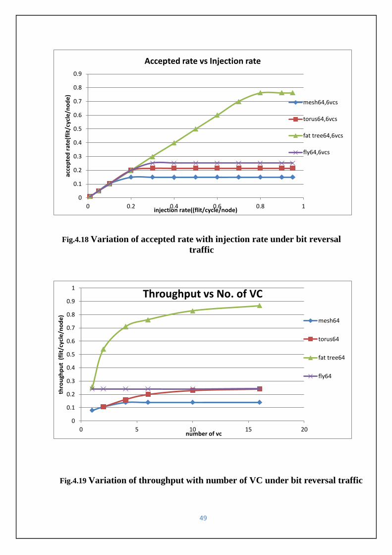
49

0

0.1

0.2

0.3

0.4

0.5

0.6

0.7

0.8

0.9

0 0.2 0.4 0.6 0.8 1

acce

pte

d r

ate

(flit

/cyc

le/n

od

e)

injection rate((flit/cycle/node)


mesh64,6vcs

torus64,6vcs

fat tree64,6vcs

fly64,6vcs

0

0.1

0.2

0.3

0.4

0.5

0.6

0.7

0.8

0.9

1

0 5 10 15 20

thro

ugh

pu

t (

flit

/cyc

le/n

od

e)

number of vc


mesh64

torus64

fat tree64

fly64

Fig.4.18 Variation of accepted rate with injection rate under bit reversal

traffic

Fig.4.19 Variation of throughput with number of VC under bit reversal traffic

50

Table4.1 saturation throughput at different number of VC for different traffic

TRAFFIC

PATERN

NO.

OF

VC

S

SATURATION THROUGHPUT(Percentage of load)

MESH 64 TORUS 64 FAT TREE 64 FLY 64

UNIFORM 2

4

6

26

36

39

22

41

51

49

70

78

52

83

88

TORNADO 2

4

6

18

24

24

8

15

18

53

70

76

24

24

24

NEIGHBOR 2

4

6

92

99

99

48

92

99

53

70

76

24

24

24

BIT COMP. 2

4

6

16

22

23

20

30

39

53

70

76

24

24

24

BIT

REVERSAL

2

4

6

10

14

14

10

15

20

54

70

76

24

24

24

In Fig.4.5 (a–c) a graph of average packet latency (load-delay curve) plotted for different

interconnect architecture with 64 nodes under uniform traffic pattern at a varying number of

VCs. Fig.4.6.shows variation of accepted rate with injection rate for 64 node for different

interconnect architecture under uniform traffic pattern. In Fig.4.7 shows variation of average

throughput (flit/cycle/node) with VC for 64 nodes for different interconnect architecture under

uniform traffic pattern.

51


interconnect architecture with 64 nodes under tornado traffic pattern at a varying number of


interconnect architecture under tornado traffic pattern. In Fig.4.10 shows variation of average


tornado traffic pattern.


interconnect architecture with 64 nodes under neighbour traffic pattern at a varying number of


interconnect architecture under neighbour traffic pattern. In Fig.4.13 shows variation of

average throughput (flit/cycle/node) with VC for 64 nodes for different interconnect

architecture under neighbour traffic pattern.


interconnect architecture with 64 nodes under bit complement traffic pattern at a varying

number of VCs. Fig.4.15.shows variation of accepted rate with injection rate for 64 node for

different interconnect architecture under bit complement traffic pattern. In Fig.4.16 shows

variation of average throughput (flit/cycle/node) with VC for 64 nodes for different

interconnect architecture under bit complement traffic pattern.


interconnect architecture with 64 nodes under bit reversal traffic pattern at a varying number of


interconnect architecture under reversal traffic pattern. In Fig.4.19 shows variation of average


reversal traffic pattern.

Table 4.1 shows saturation throughput of different interconnect architecture at different number

of VC and under different traffic pattern.

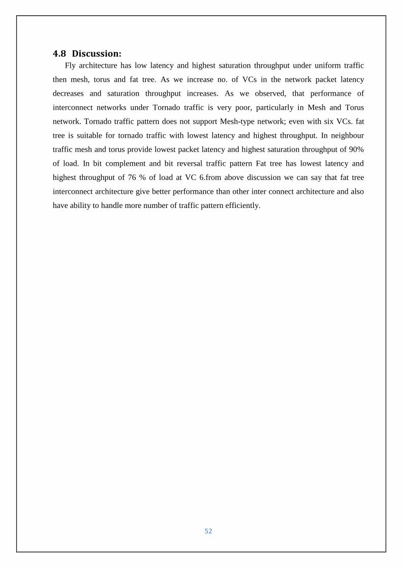
52

4.8 Discussion: Fly architecture has low latency and highest saturation throughput under uniform traffic

then mesh, torus and fat tree. As we increase no. of VCs in the network packet latency

decreases and saturation throughput increases. As we observed, that performance of

interconnect networks under Tornado traffic is very poor, particularly in Mesh and Torus

network. Tornado traffic pattern does not support Mesh-type network; even with six VCs. fat

tree is suitable for tornado traffic with lowest latency and highest throughput. In neighbour

traffic mesh and torus provide lowest packet latency and highest saturation throughput of 90%

of load. In bit complement and bit reversal traffic pattern Fat tree has lowest latency and

highest throughput of 76 % of load at VC 6.from above discussion we can say that fat tree

interconnect architecture give better performance than other inter connect architecture and also

have ability to handle more number of traffic pattern efficiently.

53

Chapter five

Performance analysis of interconnect

network on FPGA

54

In this chapter we propose a parameter based method for performance analysis of the all four

interconnect network. Performance analysis of mesh torus, fat tree and fly interconnect

architecture on chip is done by synthesis result of field programmable gate array (FPGA). The

earlier works in which NoCs are analysis in FPGA is still too small. Wolkotte et al. [2]

developed an FPGA emulator for Network-on-chip performance analysis. In this the traffic

producer was develop on an ARM processor and inserted traffic into an FPGA. In this full NoC

was emulated consecutively by implementing single router and synthesized it on FPGA.

Genako et al. [30] also develop FPGA based NoC emulator. Lee and Shannon [12] presented

application specific NoC implementation on FPGA. We analysis mesh, torus, fat tree and fly

interconnect architecture for higher number of node and see the effect of NoC parameter on

FPGA resources, clock frequency and also on path delay of network.

5.1 NoC parameter:

5.1.1 Flow control: Flow control is a process by which resources of network, such as channel bandwidth and

buffer capacity are allocated efficiently to packets. Credit based flow control [1] is used in all

interconnect network for performance analysis on FPGA.

5.1.2 Router type: There are many routers type such as input queued router which is simplest type of router

and offer lowest performance, virtual channel router offer best performance so we select virtual

channel router.

5.1.3 Virtual channels: Virtual channel basically use for removing head of line blocking probability but this

increase area of network. We varied the number of VC from 2 to 6 and measure the resource

utilization of FPGA.

5.1.4 Flit data width: Flit data width defines by the size of data in bits. It contains one extra bit for flow control

and bookkeeping purpose. When the value of flit data width increase then FPGA resource uses

also increases.

55

5.1.5 Flit buffer depth: The size of flit buffer in flit is called flit buffer depth. Larger buffer offer beater

performance under heavy load.

5.2 Experimental setup: We designed a different NoC configuration using [14] and synthesis the NoC configuration

using Xilinx 14.2 on vertex7 board. Vertex7 has higher no. of resources so it can be used to

implement for higher no. of node NoC. The synthesis result includes PLUT (% look up table)

maximum clock frequency. Critical path delay of different interconnects NoC network

determines by Xilinx timing analyser. Here critical path delay is sum of offset in and offset out

of FPGA device. We use following NOC parameter

virtual channel router

credit based flow control

separable input first round robin allocator

use pipelining

use virtual link

use pipelining router core

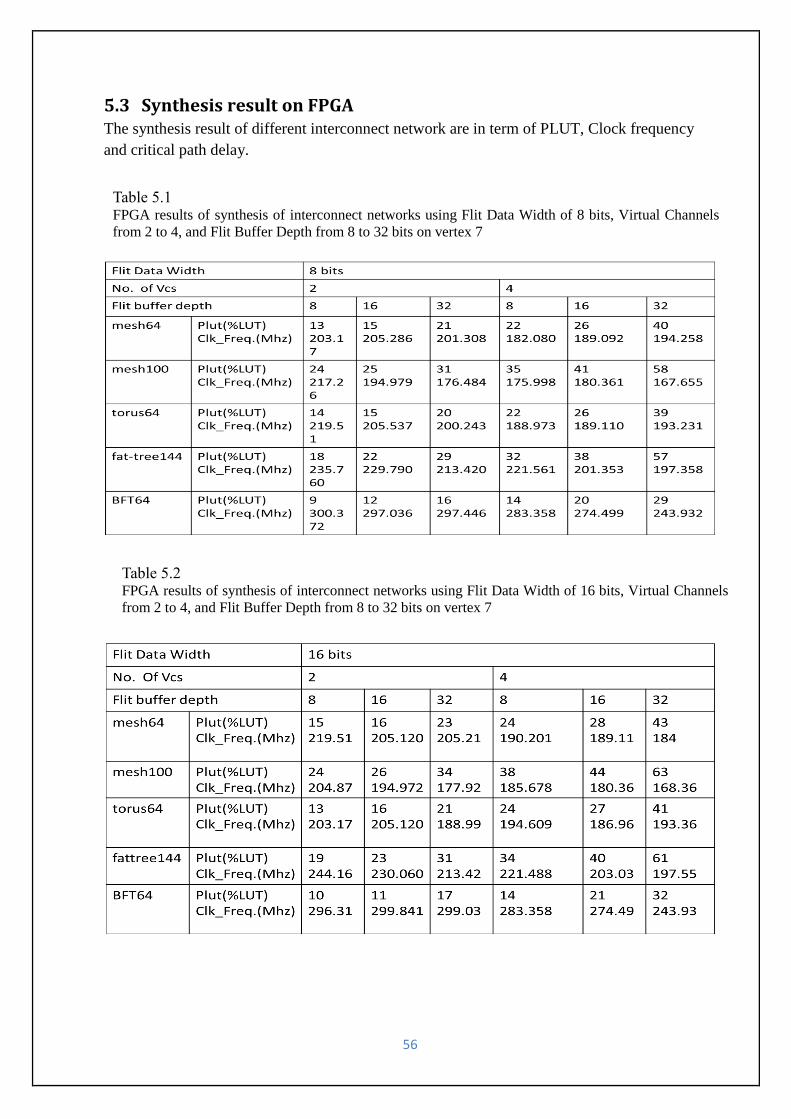
56

5.3 Synthesis result on FPGA The synthesis result of different interconnect network are in term of PLUT, Clock frequency

and critical path delay.

Table 5.1 FPGA results of synthesis of interconnect networks using Flit Data Width of 8 bits, Virtual Channels

from 2 to 4, and Flit Buffer Depth from 8 to 32 bits on vertex 7



57



Table 5.4

Path delay of different interconnect network with Flit Data Width of 8 bits, VCs from 2 to 4, and Flit

Buffer Depth from 8 to 32 bits on the Virtex-7 FPGA .

58

Table 5.5


Buffer Depth from 8 to 32 bits on the Virtex-7 FPGA.

Table 5.6


Buffer Depth from 8 to 32 bits on the Virtex-7 FPGA.

59

Table 5.1 to 5.3 shows PLUT and maximum clock frequency of different interconnect

architecture at different no. of VCs. Table 5.4 to 5.6 shows critical path delay of different

interconnect architecture

5.4 Discussion: Synthesis result of different interconnect network on FPGA with different NoC parameter

observed in term of PLUT and clock frequency. In this experiment we vary flit data width and

flit buffer depth from 8 to 32bits and VCs from 2 to 4. Table5.1 to 5.3 show synthesis result of

mesh torus fat tree, bft network.

According to the above result we can observed that when no. of nodes of mesh interconnect

increase then PLUT increase and clock frequency increases when flit buffer depth increases

then clock frequency increases and when flit data width increases then clock frequency

increases. in fat tree and bft interconnect network when flit buffer depth and flit data width

increases then clock frequency decreases so bft and fat tree is use at low value of flit data width

and flit buffer depth .table5.4 to 5.6 show critical path delay who vary with no, of VCs and flit

data width. Bft has lowest critical path delay. Among all interconnect network BFT network

has highest clock frequency and low critical path delay but it has low saturation throughput as

seen in table4.1 so fat tree interconnect network is best among all in term of latency saturation

throughput and also better in term of clock frequency then mesh and torus.

60

Chapter six

Power and area analysis of interconnect

network

61

Now a day’s power and area analysis is important recherché area in NoC and also key concern

in on chip design. Its effect on performance and reliability of on chip network if power

requirement fail means complete chip fail.

6.1 Power dissipation: The total power dissipated by a network divide into two categories: static power is the

power dissipated when the network is on off state, and dynamic power denotes the power

consumed by switching logic in the circuit.

6.1.1 Static power:

Static power is dissipated in numerous methods.

Static dissipation due to „ sub threshold conduction through OFF transistors „

Tunnelling current through gate oxide

leakage through reverse-biased diodes „

contention current in rationed circuits

Where V supply voltage leakage current

6.1.2 Dynamic power: Dynamic power is dissipated due to charging and discharging of load and internal capacitor

and short circuit current while both PMOS and NMOS networks are partly ON .The dynamic

power dissipated within the circuit is generally categorized as the internal power and switching

power

6.1.2.1 Switching power:

The switching power is determined by the capacitive load and the frequency of the logic

transitions on a circuit output.

62

Where totals load capacitor and f frequency of switching

6.1.2.2 Internal power:

The internal power is produced by the charging of inside capacitor loads as well as by the

short-circuit current between the NMOS and PMOS transistors of a gate when both are on.

(

)

Where total internal capacitors

Short circuit current

Supply voltage

6.2 Area: Interconnect network area basically occupy by router and links. Area of chip is depending upon

gate size of transistor. The cost of NoC design depends upon area.

6.3 Experimental setup: For power and area analysis we use synopsis tool [31] and use 65 nm technologies for area and

power calculation.

Flit data width of 8 flits

Voltage unit = 1v

Capacitance =1 pf

63

0

20

40

60

80

100

120

140

bd=8 bd=16 bd=32

Tota

l P

ow

er(m

w)

internal power switchinng power leakage power

6.4 Results: Power analysis of different interconnect is shown below in this we measure power by varying

buffer depth and number of VCs and we also analysis area of different interconnect network .

Fig.6.1 total power at different buffer depth of mesh interconnect network at VC2

64

0

20

40

60

80

100

120

140

160

bd=8 bd=16 bd=32

Tota

l po

wer

(mw

) internal power switching power Series leakage power

0

20

40

60

80

100

120

140

bd=8 bd=16 bd=32

Tota

l po

wer

(mw

)

internal power switching power leakage power

Fig.6.2 total power at different buffer depth of mesh interconnect network at VC4

Fig.6.3 Total power at different buffer depth of torus interconnect network at VC2

65

0

20

40

60

80

100

120

140

160

180

bd=8 bd=16 bd=32

Tota

l po

wer

(mw

)


0

20

40

60

80

100

120

bd=8 bd=16 bd=32

Tota

l po

wer

(mw

)


Fig.6.4 Total power at different buffer depth of torus interconnect network at VC4

Fig.6.5 Total power at different buffer depth of Fat tree interconnect network at VC2

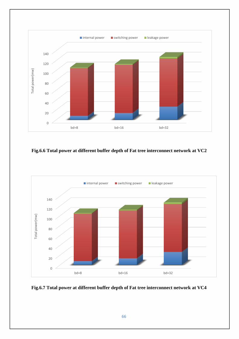
66

0

20

40

60

80

100

120

140

bd=8 bd=16 bd=32

Tota

l po

wer

(mw

)


0

20

40

60

80

100

120

140

bd=8 bd=16 bd=32

Tota

l po

wer

(mw

)




67

0

20

40

60

80

100

120

bd=8 bd=16 bd=32

Tota

l po

wer

(mw

) internal power switching power leakage power

0

20

40

60

80

100

120

140

bd=8 bd=16 bd=32

Tota

l po

wer

(um

)

leakage power switching power internal power

Fig.6.8 Total power at different buffer depth of butter fly interconnect network at VC2

Fig.6.9 Total power at different buffer depth of butter fly interconnect network at VC4

68

0

200000

400000

600000

800000

1000000

1200000

1400000

1600000

bd=8 bd=16 bd=32

AR

EA( 𝜇𝑚

)^2

mesh torus fat tree fly

0

100000

200000

300000

400000

500000

600000

700000

800000

900000

bd=8 bd=16 bd=32

AR

EA(𝜇𝑚

)^2

mesh torus fat tree fly

Fig.6.10 Area compression of different interconnect network at VC2

Fig.6.11 Area compression of different interconnect network at VC4

69

mesh vc2

mesh vc40

500000

1000000

1500000

2000000

bd=8bd=16

bd=32

mesh vc2

mesh vc4

0

20

40

60

80

100

120

140

160

180

0 5 10 15 20 25 30 35

TOTA

L P

OW

ER(M

W)

BUFFET DEPTH

meshvc2 torus vc2 fat tree vc2 fly vc2 mesh vc4

Fig.6.12 Total power varying with buffer depth of different interconnect network

Fig.6.13 Area varying with buffer depth of mesh interconnect network

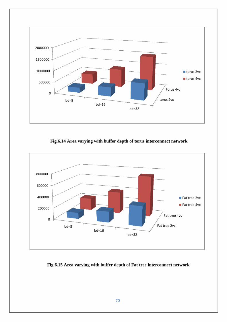
70

torus 2vc

torus 4vc0

500000

1000000

1500000

2000000

bd=8bd=16

bd=32

torus 2vc

torus 4vc

Fat tree 2vc

Fat tree 4vc0

200000

400000

600000

800000

bd=8bd=16

bd=32

Fat tree 2vc

Fat tree 4vc

Fig.6.14 Area varying with buffer depth of torus interconnect network

Fig.6.15 Area varying with buffer depth of Fat tree interconnect network

71

Fig.6.1 to Fig.6.9 shows histogram of total power of different interconnect network at vc2 and

vc4 with varying buffer depth. This histogram made by combining all three power internal

power, switching power, leakage power.

Fig.6.10 and Fig.6.11 shows histogram of area compression of all interconnect network at vc2

and vc4 with varying buffer depth.

Fig.6.12 show variation of total power with buffer depth of all interconnect network at vc2 and

vc4.

Fig.6.13 to Fig.6.16show area histogram at vc2 and vc4 of all interconnect network.

fly 2vc

fly 4vc0

100000

200000

300000

400000

500000

600000

700000

bd=8bd=16

bd=32

fly 2vc

fly 4vc

Fig.6.16 Area varying with buffer depth of Fat tree interconnect network

72

6.5 Discussion:

In this chapter we calculate total power and area of all interconnect by varying buffer depth

at vc2 and vc4. In fig.6.1 to fig.6.9 we can see that if buffer depth increases internal power

increases by large amount but switching and leakage power increases slightly. In total power

majority component of power is switching power that is dynamic power. Total power also

increases if we increase number of VCs. In Fig.6.12 total power vary linearly with buffer depth.

In Fig.6.12 we can see that butterfly and fat tree at vc2 has lowest power variation with buffer

depth among all interconnect network. From this we can concluded that fat tree and butter fly

interconnect network with vc2 have lest power dissipation among all interconnect but butter fly

has low saturation throughput in compare to fat tree as seen in Table 4.1so Fat tree interconnect

network is best among all interconnect network. In fig.6.10 and fig.6.10 we can see that area of

fat tree and butterfly is very low then mesh and torus network. In fig6.13 to fig.6.16 we can see

that if number of VCs increases then area of network also increases if area increases then cost

of network also increases. Fat tree interconnect network has lowest area among all

interconnect network. So fat tree network interconnect network is suitable for NoC.

73

Chapter seven

Conclusion and future work

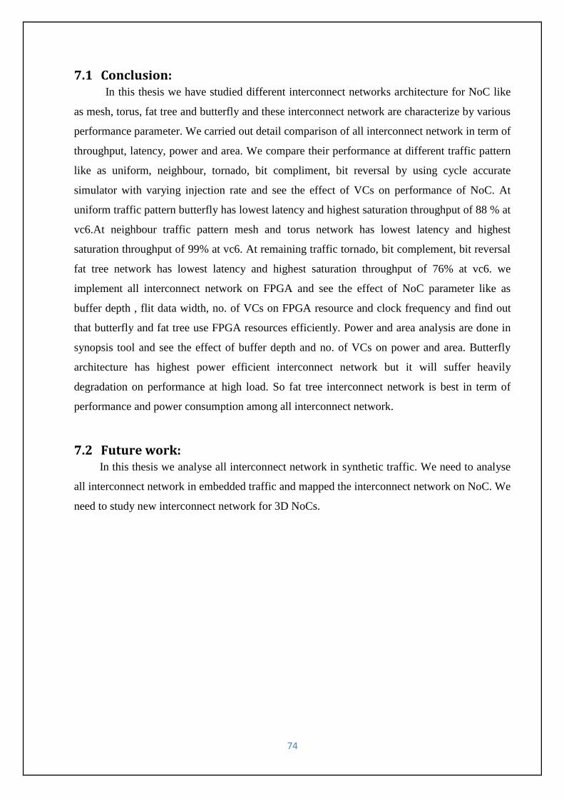
74

7.1 Conclusion: In this thesis we have studied different interconnect networks architecture for NoC like

as mesh, torus, fat tree and butterfly and these interconnect network are characterize by various

performance parameter. We carried out detail comparison of all interconnect network in term of

throughput, latency, power and area. We compare their performance at different traffic pattern

like as uniform, neighbour, tornado, bit compliment, bit reversal by using cycle accurate

simulator with varying injection rate and see the effect of VCs on performance of NoC. At

uniform traffic pattern butterfly has lowest latency and highest saturation throughput of 88 % at

vc6.At neighbour traffic pattern mesh and torus network has lowest latency and highest

saturation throughput of 99% at vc6. At remaining traffic tornado, bit complement, bit reversal

fat tree network has lowest latency and highest saturation throughput of 76% at vc6. we

implement all interconnect network on FPGA and see the effect of NoC parameter like as

buffer depth , flit data width, no. of VCs on FPGA resource and clock frequency and find out

that butterfly and fat tree use FPGA resources efficiently. Power and area analysis are done in

synopsis tool and see the effect of buffer depth and no. of VCs on power and area. Butterfly

architecture has highest power efficient interconnect network but it will suffer heavily

degradation on performance at high load. So fat tree interconnect network is best in term of

performance and power consumption among all interconnect network.

7.2 Future work: In this thesis we analyse all interconnect network in synthetic traffic. We need to analyse

all interconnect network in embedded traffic and mapped the interconnect network on NoC. We

need to study new interconnect network for 3D NoCs.

75

References

[1] W. Dally and B. Towles, “Principles and practices of interconnection Network”, Morgan

Kaufmann, 2004.

[2] N.E.jerger and L.S.peh, On-chip Network: “Synthesis lectures on computer architecture”,

Morgan and Claypool, 2009.

[3] K. Shuler, "The SoC Interconnect Fabric: A Brief History," Arteris Connected Blog,

2013

[4] W.J. dally, B.towels, Route Packets, Not Wires: “On-Chip Interconnection Networks”,

Design Automation Conference, 2001. Proceedings, pp. 684-689.

[5] L. Benini and G. DeMicheli, Networks on Chips: “A New SoC Paradigm,” Computer

architecture 2002, volume no. 35, pp. 70-78.

[6] P. Magarshack and P.G.Paulin, “System-on-Chip beyond the Nanometre Wall,”

Processes Design Automation Conference (DAC), pp. 419-424, 2003.

[7] M. Horowitz and B. Dally, “How Scaling Will Change Processor Architecture,”

Processes Int’l Solid State Circuits Conference. (ISSCC), 2004, pp. 132-133.

[8] X. Ju, L. Yang, “Performance analysis and comparison of 2 x 4 network on chip

topology”, Microprocessor. Microsystem. Journal 2012 pp. 505–509.

[9] S. Kundu, J. Sounya, S. Chattopadhyay, “Design and evaluation of mesh-of-tree based

network-on-chip using virtual channel router”, Microprocessor Microsystem. Journal

2012, pp.471–488.

[10] M.S. Abdel Fattah, V. Betz, “Design Trade-offs for hard and Soft FPGA-based Networks

on-Chip”, in: an 11th International Conference on Field Programmable Technology

(FPT11), 2012, pp. 95–103.

[11] J. Lee, L. Shannon, “The effect of node size, heterogeneity, and network size on FPGA

based NoCs”,: an International Conference on Field-Programmable Technology (FPT),

2009, pp. 479–482.

[12] J. Lee, L. Shannon, “Predicting the performance of application-specific NoCs

implemented on FPGAs”,: Nineteenth ACM/SIGDA International Symposium on Field-

Programmable Gate Arrays (FPGA), 2011, pp. 23–32.

[13] S. Abba, J. Lee, “Examining the performance impact of NoC parameters for scalable and

adaptive FPGA-based network-on-chips”,: IEEE Fifth International Conference on

Computational Intelligence, Modelling and Simulation (CIMSim), IEEE Computer

Society, 2013, pp. 364–372.

[14] M.K. Papamichael, J.C. Hoe, CONNECT: “Re-examining Conventional Wisdom of

Designing NoCs in the Context of FPGAs”, FPGA 12 ACM, 2012, pp. 37–46.

[15] N. Jiang et al., “A detailed and flexible cycle-accurate network-on-chip simulator”,:

IEEE International Symposium on Performance Analysis of Systems and Software

(ISPASS), 2013, pp. 86–96.

[16] G. Schelle, D. Grunwald, “On chip interconnect exploration for multicore processors

utilizing FPGAs”, 2nd Workshop on Architecture Research using FPGA Platforms

(WARFP), 2006.

[17] P.P. Pande, C.G. Grecu, M. Jones, A. Ivanor, R. Saleh, “Performance evaluation and

design trade-offs for network-on-chip interconnect architectures”, IEEE Transaction on

Computer architecture, 2005 pp. 1025–1040.

[18] S.abba, Jeong a lee, “A parametric-based performance evaluation and design trade-offs

for interconnect architectures using FPGAs for networks-on-chip”, Microprocessors and

Microsystems journal 2014, pp. 375–398.

http://ieeexplore.ieee.org/xpl/mostRecentIssue.jsp?punumber=7445

76

[19] M.E. Kreutz, C.M. Marcon, L. Carro, F. Wagner, A.A. Susin, Design space exploration

comparing homogeneous and heterogeneous network-on-chip architectures, in: Proc.

SBCCI, 2005.

[20] M. A. Yogita A. Sadawarte, “Comparative Study of Switching Techniques for Network-

on-Chip Architecture,” in ICCCS’11, Rourkela, 2011.

[21] N. Jiang et al., “BookSim interconnection network simulator,” Online,

https://nocs.stanford.edu/cgibin/trac.cgi/wiki/Resources/BookSim.

[22] L. Jain et al., “NIRGAM - a simulator for NoC interconnect routing and application

modeling,” Online,http://nirgam.ecs.soton.ac.uk/.

[23] P. K. Sahu and S. Chattopadhyay. “A survey on application mapping strategies for

Network-on-Chip design”, Journal of System Architecture 2013, pp. 60-76.

[24] S. Y. Jose Duato, Interconnection Networks: “An engineering approach”, New York:

Morgan Kaufmann Publishers, 2010.

[25] J. Hennessey and D. Patterson, Computer Architecture: “A Quantitative Approach”.

Morgan Kaufmann, 2003.

[26] J. Kim, C. Nicopoulos, D. Park, “A gracefully degrading and energy-efficient modular

router architecture for on-chip networks”, SIGARCH Computer Architecture News

2006, pp. 4–15.

[27] S. Coll, F.J. Mora, J. Duato, F. Petrini, “Efficient and scalable hardware-based multicast

in fat-tree networks”, IEEE Transactional Parallel Distributed System 2009, pp.1285–

1298.

[28] Skeie, T. Sem-Jacobsen, F.O. Rodrigo, S. Flich, J. Bertozzi, D. Medardoni, S. ,

“Flexible DOR routing for virtualization of multicore chips,” System-on-Chip, 2009.

SOC 2009. International Symposium

[29] P.T. Wolkotte, K.F. Hölzenspies, J.M.Smit, Fast, accurate and detailed NoC simulations,

in: Process International Symposium on Networks-on-Chip, 2007, pp. 323–333.

[30] Genko, D. Atienza, G. De Micheli, J.M. Mendias, R. Hermida, F. Catthoor, A complete

network-on-chip emulation framework””, in: Process Design, Automation and Test,

2005, pp. 246–251.

[31] http://www.synopsys.com/Tools/Verification/hardwareverification/emulation/Pages/defa

ult.aspx.

https://nocs.stanford.edu/cgibin/trac.cgi/wiki/Resources/BookSim

http://ieeexplore.ieee.org/search/searchresult.jsp?searchWithin=p_Authors:.QT.Skeie,%20T..QT.&searchWithin=p_Author_Ids:37273563800&newsearch=true

http://ieeexplore.ieee.org/search/searchresult.jsp?searchWithin=p_Authors:.QT.Sem-Jacobsen,%20F.O..QT.&searchWithin=p_Author_Ids:38286716100&newsearch=true

http://ieeexplore.ieee.org/search/searchresult.jsp?searchWithin=p_Authors:.QT.Rodrigo,%20S..QT.&searchWithin=p_Author_Ids:37531310000&newsearch=true

http://ieeexplore.ieee.org/search/searchresult.jsp?searchWithin=p_Authors:.QT.Flich,%20J..QT.&searchWithin=p_Author_Ids:37272659300&newsearch=true

http://ieeexplore.ieee.org/search/searchresult.jsp?searchWithin=p_Authors:.QT.Bertozzi,%20D..QT.&searchWithin=p_Author_Ids:37274635000&newsearch=true

http://ieeexplore.ieee.org/search/searchresult.jsp?searchWithin=p_Authors:.QT.Medardoni,%20S..QT.&searchWithin=p_Author_Ids:37317914900&newsearch=true

Performance Analysis of Different Interconnect Networks ...

Documents

Transcript of Performance Analysis of Different Interconnect Networks ...