Perfect Competition & Welfare

Outline

Derive aggregate supply functionShort and Long run equilibriumPractice problemConsumer and Producer SurplusDead weight lossPractice problem

Focus on profit maximizing behavior of firmsTake as given the market demand curve

Equation:P = A - B.Q

lineardemand

Equation:P = A - B.Q

lineardemand

Inverse demand function:willingness to pay

Maximum willingnessto pay

Maximum willingnessto pay

$/unit

Quantity

A

A/B

Demand

P1

Q1

Constantslope

Constantslope

At price P1 a consumerwill buy quantity Q1

At price P1 a consumerwill buy quantity Q1

Perfect Competition

Firms and consumers are price-takersFirm can sell as much as it likes at the ruling market price

do not need many firmsdo need the idea that firms believe that their actions will not affect the market price

Therefore, marginal revenue equals priceTo maximize profit a firm of any type must equate marginal revenue with marginal costSo in perfect competition price equals marginal cost

MR = MC

Profit is π(q) = R(q) - C(q)Profit maximization: dπ/dq = 0This implies dR(q)/dq - dC(q)/dq = 0But dR(q)/dq = marginal revenue

dC(q)/dq = marginal costSo profit maximization implies MR = MC

Perfect competition: an illustration

$/unit

Quantity

$/unit

Quantity

D1S1

QC

AC

MC

PCPC

(b) The Industry(a) The Firm With market demand D1and market supply S1

equilibrium price is PCand quantity is QC

With market demand D1and market supply S1

equilibrium price is PCand quantity is QC

With market price PCthe firm maximizes

profit by settingMR (= PC) = MC andproducing quantity qc

With market price PCthe firm maximizes

profit by settingMR (= PC) = MC andproducing quantity qc

qc

D2

Now assume thatdemand

increases toD2

Now assume thatdemand

increases toD2

Q1

P1P1

With market demand D2and market supply S1

equilibrium price is P1and quantity is Q1

With market demand D2and market supply S1

equilibrium price is P1and quantity is Q1

q1

Existing firms maximize profits by increasing

output to q1

Existing firms maximize profits by increasing

output to q1

Excess profits inducenew firms to enter

the market

Excess profits inducenew firms to enter

the market

• The supply curve moves to the right

• Price falls

• Entry continues while profits exist

• Long-run equilibrium is restoredat price PC and supply curve S2

S2

Q´C

Perfect competition: additional pointsDerivation of the short-run supply curve

this is the horizontal summation of the individual firms’marginal cost curves

Example 1: Three firms

Firm 1: MC = 4q + 8

Firm 2: MC = 2q + 8

Firm 3: MC = 6q + 8

Invert these

Aggregate: Q= q1+q2+q3= 11MC/12 - 22/3

MC = 12Q/11 + 8

Firm 1: q = MC/4 - 2

Firm 2: q = MC/2 - 4

Firm 3: q = MC/6 - 4/3

Firm 1Firm 3

Firm 2

q1+q2+q3

$/unit

Quantity

8

Example 2: Eighty firms

Each firm: MC = 4q + 8

Invert these

Each firm: q = MC/4 - 2

Aggregate: Q= 80q = 20MC - 160

MC = Q/20 + 8

Firm i$/unit

Quantity

8

Definition of normal profitnot the same as zero profitimplies that a firm is making the market return on the assets employed in the business

Aggregate

Practice problem

( ) qqqTC

QPDemandInverse

PQDemand

D

D

101005090120:

9506000:

2 ++=

−=

−=

Initial number of firms = 20

1) Find short run equilibrium

2) Find long run equilibrium

Short run

( )

3.49140

69009

50600010010

100102

10102

101009

506000

2

≈=

−=−⇒=

−=

−=

+=++=

−=

p

ppSD

pQ

pq

qmcqqqTC

PQ

s

s

D

Long run

P = min avg costPoint at which MC=AC

5010/500/

5009

45009

50600030

10

10100102

10100102

===⇒=

==−

=

==

++=+⇒=

++=

+=

qQnQnq

pQ

pq

qq

qacmc

qq

ac

qmc

Exercise

Competitive Industry – 2 types of firms

1. Low cost firms:

• Constant marginal cost 10 cents per unit – no fixed cost.

• Total capacity of group = 1000 units

2. High cost firms:

• marginal cost of 20 cents per unit

• When producing at full capacity average cost = 30 cents

• total group capacity of 2000 units

a) Draw the long run supply curve of this industry and the short run

supply curve assuming all firms are active.

(b) After a fall in demand, there has been an initial price reduction inthe short run, followed by a price increase in the long run. Drawdemand curves before and after the fall in demand that would leadto this situation. Explain.

(c) Consider again the initial situation and suppose the low cost firmsdiscover extra capacity (e.g. new oil wells) at the same marginal costof 10 cents per unit and that in the short run this lead to a reductionin price but in the long run the price returned to its previous level.Draw a picture for the supply function of this industry prior andafter the change and the demand function that would explain thissituation.

Efficiency and Surplus

Can we reallocate resources to make some individuals better off without making others worse off?Need a measure of well-being

consumer surplus: difference between the maximum amount a consumer is willing to pay for a unit of a good and the amount actually paid for that unitaggregate consumer surplus is the sum over all units consumed and all consumersproducer surplus: difference between the amount a producer receives from the sale of a unit and the amount that unit costs to produceaggregate producer surplus is the sum over all units produced and all producers total surplus = consumer surplus + producer surplus

Quantity

$/unit

Demand

Competitive Supply

PC

QC

The demand curve measures the willingness to pay for each unitConsumer surplus is the area between the demand curve and the equilibrium price

Consumer surplusThe supply curve measures the

marginal cost of each unitProducer surplus is the area between the supply curve and the equilibrium price

Producer surplus

Aggregate surplus is the sum of consumer surplus and producer surplus

Equilibrium occurswhere supply equalsdemand: price PC

quantity QC

Equilibrium occurswhere supply equalsdemand: price PC

quantity QC

Efficiency and surplus: illustration

The competitive equilibrium is efficient

Illustration (cont.)

Quantity

Demand

Competitive Supply

QC

PC

$/unitAssume that a greater quantity QGis tradedPrice falls to PG

QG

PG

Producer surplus is now a positive partand a negative part

Consumer surplus increases

Part of this is a transfer from producersPart offsets the negative producer surplus

The net effect is a reduction in total surplus

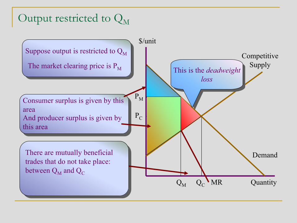
Output restricted to QM

Demand

Competitive Supply

QC

PC

$/unit

MR Quantity

Suppose output is restricted to QM

The market clearing price is PM

QM

PMConsumer surplus is given by this areaAnd producer surplus is given by this area

There are mutually beneficial trades that do not take place: between QM and QC

This is the deadweightloss

This is the deadweightloss

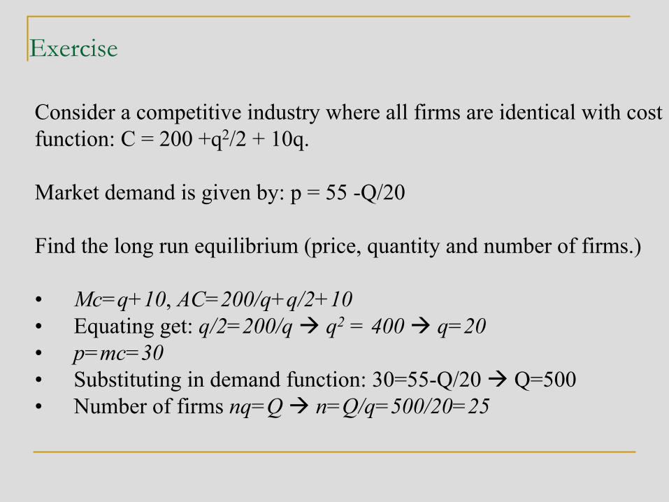
Exercise

Consider a competitive industry where all firms are identical with costfunction: C = 200 +q2/2 + 10q.

Market demand is given by: p = 55 -Q/20

Find the long run equilibrium (price, quantity and number of firms.)

• Mc=q+10, AC=200/q+q/2+10• Equating get: q/2=200/q q2 = 400 q=20• p=mc=30• Substituting in demand function: 30=55-Q/20 Q=500• Number of firms nq=Q n=Q/q=500/20=25

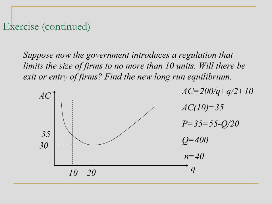
Exercise (continued)

Suppose now the government introduces a regulation that limits the size of firms to no more than 10 units. Will there beexit or entry of firms? Find the new long run equilibrium.

q

AC

20

30

10

AC=200/q+q/2+10

AC(10)=35

P=35=55-Q/20

Q=400

n=40

35

Exercise (continued)

Suppose now the government introduces a regulation that forces firms to produce no less than 40 units. Find the new long run equilibrium.

q

AC

20

30

40

AC=200/q+q/2+10

AC(40)=35

P=35=55-Q/20

Q=400

n=10

35

Exercise (continued)

Welfare cost:

Q

Qs3035

Welfare loss

500400

Welfare loss:

5*400+100*5/2

=2,250

Original Surplus:

500*25/2=6,250

% loss = 36%

55