Perceptron Learning Algorithm (PLA)kuh/ee645.f12/slides/ee645-5.pdf · QP software for SVM •...

Department of Electrical

Engineering

Lecture 5: Aug. 29, 2012

Review: Lecture 4 •  Perceptron Learning Algorithm (PLA)

–  Learning algorithm for linear threshold functions (LTF) (iterative)

–  Energy function: PLA implements a stochastic gradient algorithm

–  Novikoff’s theorem (algebraic proof bounding number of updates, depends on margins)

–  Version space (set of points where weights classify all training points correctly)

–  Solution is ill posed, formulate optimization problem based on margins

1


Engineering


Optimum Margin Classifiers

Consider methods based on optimum margin classifiers or Support Vector Machines (SVM)

Here we consider a different algorithm that is well

posed with a unique optimal solution. The solution is based on finding the largest minimal margin of all training points.

2


Engineering


Optimal Marginal Classifiers

X

X X

O O

O

Given a set of points that are linearly separable:

which hyperplane should you choose to separate points?

Choose hyperplane that maximizes distance between two sets of points.

X

3


Engineering


Finding Optimal Hyperplane

X

X X

O O

O

X 1) Draw convex hull around each set of points.

2) Find shortest line segment connecting two convex hulls.

3) Find midpoint of line segment.

4) Optimal hyperplane is perpendicular to segment at midpoint of line segment.

w

margins

Optimal hyperplane

4


Engineering


Alternative Characterization of Optimal Margin Classifiers

X

X X

O O

O

X

u

v

w

Maximizing margins equivalent to minimizing magnitude of weight vector.

W u+ b = 1 T

W v+ b = -1 T

2m

W (u-v) = 2 T

W (u-v)/ W = 2/ W =2m T

5


Engineering


Quadratic Programming Problem

Problem statement: max (w,b) min (||x-x(i) ||) : x ∈ R n , wT x + b = 0, 1 ≤ i ≤l which is equivalent to solving (QP) problem:

Min ½||w||2

subject to di (wT x(i) + b) ≥ 1, ∀i

6


Engineering


Lagrange Multipliers

Constrained optimization can be dealt with by

introducing Lagrange multipliers α(i) ≥ 0 and augmenting objective function

L(w,b,α) = ½||w||2 - Σ α(i) (d(i) (wT x(i) + b) –1)

7


Engineering


Support Vectors

QP program is convex and note that at solution ∂L(w,b,α) / ∂w =0 and ∂L(w,b,α) / ∂b = 0 leading to Σ α(i) d(i) = 0 and w = Σ α(i) d(i) x(i) Weight vector expressed in terms of subset of training

vectors xi and αi that are nonzero. These are support vectors. By KKT conditions we have that

α(i) (d(i) (wT x(i) + b) –1) = 0 indicating that support vectors lie on margin.

8


Engineering


Support Vectors

X

X X

O O

O

Points in red are support vectors.

X

9


Engineering


Dual optimization representation

Solving the primal QP problem is equivalent to solving the dual QP problem. Primal variables w, b are eliminated.

max W(α) = Σ α(i) - ½Σ α(i) α(j) d(i) d(j)(x(i)

Tx(j) ) subject to α(i) ≥ 0, and Σ α(i) d(i) = 0 . The hyperplane decision function can be written as

f(x) = sgn (Σ α(i) d(i) xT x(i) + b)

10


Engineering


Comments about SVM solution

•  Solution can be found in primal or dual spaces. When we discuss kernels later there are advantages of finding solution in dual space.

•  Threshold, b is determined after weight w is found. •  In version space, SVM solution is center of largest

hypersphere that fits in version space. •  Solution can be modified to

–  Handle training data that is not linearly separable via slack variables

–  Implement nonlinear discriminant function via kernels •  Solving quadratic programming problems

11


Engineering


Handling data that not linearly separable

•  Data is often noisy or inconsistent resulting in training data being not linearly separable.

•  PLA algorithm can be modified (pocket algorithm), however there are problems with algorithm termination.

•  SVM can easily handle this case by adding slack variables to handle pattern recognition.

12


Engineering


Training examples below margin

X

X X

O O

O

X

w

margins

Optimal hyperplane x

O

13


Engineering


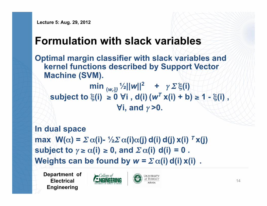
Formulation with slack variables Optimal margin classifier with slack variables and

kernel functions described by Support Vector Machine (SVM).

min (w,ξ) ½||w||2 + γ Σ ξ(i) subject to ξ(i) ≥ 0 ∀i , d(i) (wT x(i) + b) ≥ 1 - ξ(i) ,

∀i, and γ >0. In dual space max W(α) = Σ α(i)- ½Σ α(i)α(j) d(i) d(j) x(i) T x(j) subject to γ ≥ α(i) ≥ 0, and Σ α(i) d(i) = 0 . Weights can be found by w = Σ α(i) d(i) x(i) .

14


Engineering


Solving QP Problem •  Quadratic programming problem with linear

inequality constraints. •  Optimization problem involves searching space of

feasible solutions (points where inequality constraints satisfied).

•  Can solve problem in primal or dual space.

15


Engineering


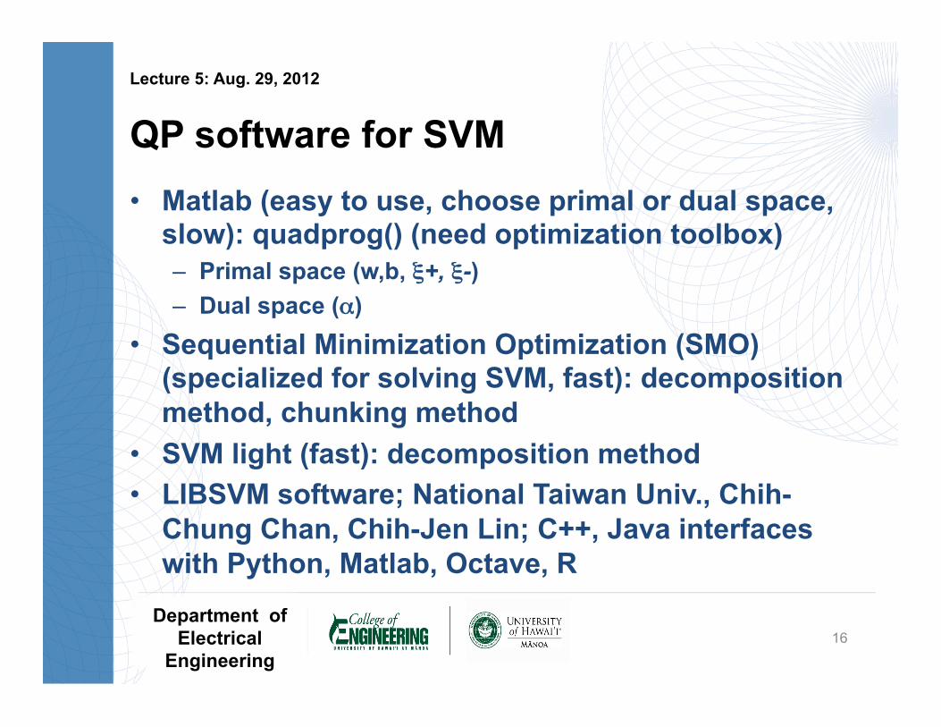
QP software for SVM •  Matlab (easy to use, choose primal or dual space,

slow): quadprog() (need optimization toolbox) –  Primal space (w,b, ξ+, ξ-) –  Dual space (α)

•  Sequential Minimization Optimization (SMO) (specialized for solving SVM, fast): decomposition method, chunking method

•  SVM light (fast): decomposition method •  LIBSVM software; National Taiwan Univ., Chih-

Chung Chan, Chih-Jen Lin; C++, Java interfaces with Python, Matlab, Octave, R

16


Engineering


Example

Drawn from Gaussian data cov(X) = I

20 + pts. Mean = (.5,.5) 20 - pts. Mean = -(.5,.5)

17


Engineering


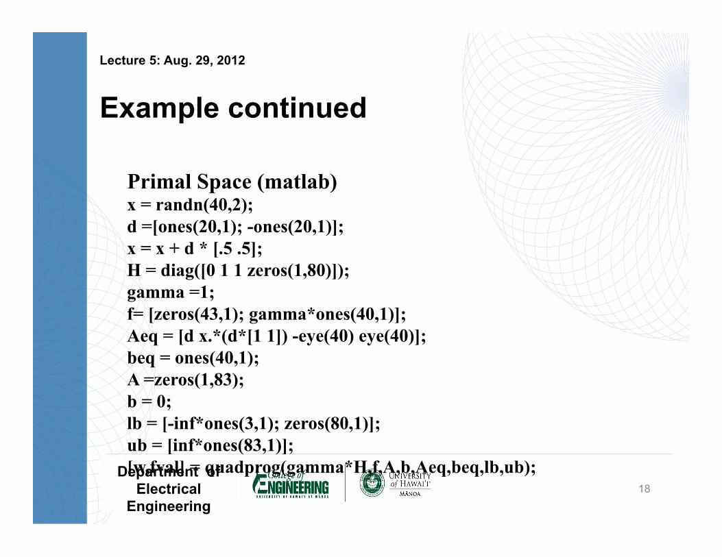
Example continued

Primal Space (matlab) x = randn(40,2); d =[ones(20,1); -ones(20,1)]; x = x + d * [.5 .5]; H = diag([0 1 1 zeros(1,80)]); gamma =1; f= [zeros(43,1); gamma*ones(40,1)]; Aeq = [d x.*(d*[1 1]) -eye(40) eye(40)]; beq = ones(40,1); A =zeros(1,83); b = 0; lb = [-inf*ones(3,1); zeros(80,1)]; ub = [inf*ones(83,1)]; [w,fval] = quadprog(gamma*H,f,A,b,Aeq,beq,lb,ub);

18


Engineering


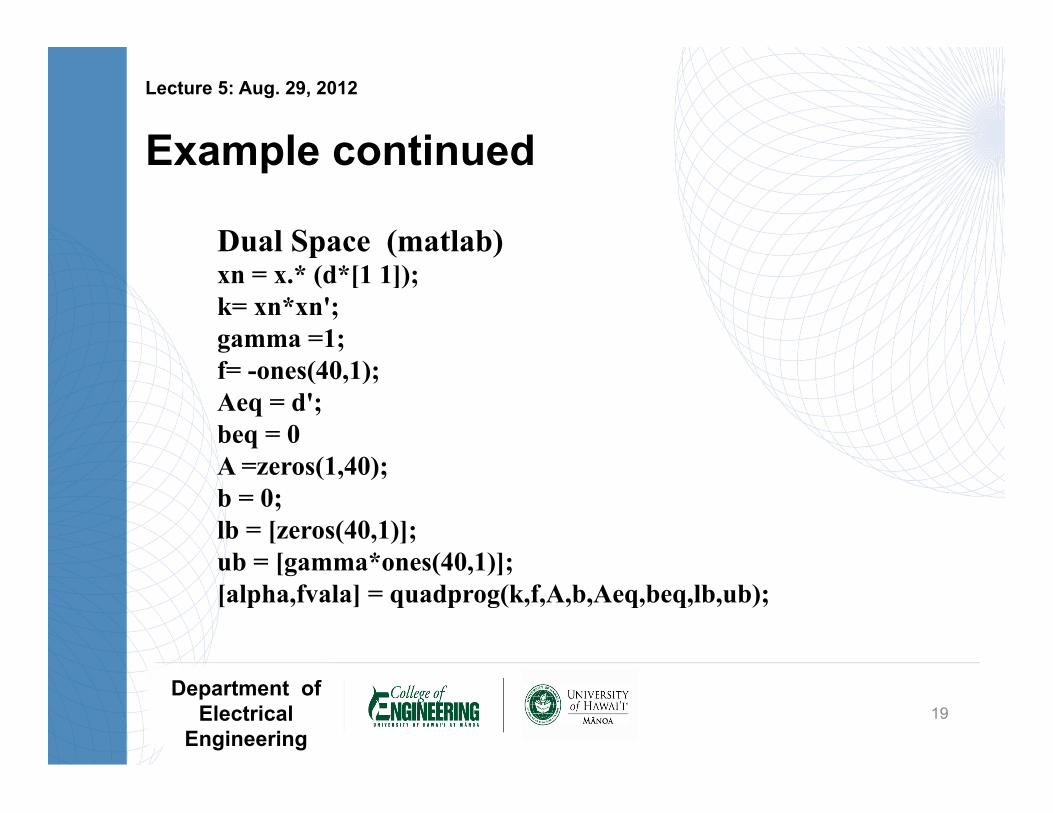
Example continued

Dual Space (matlab) xn = x.* (d*[1 1]); k= xn*xn'; gamma =1; f= -ones(40,1); Aeq = d'; beq = 0 A =zeros(1,40); b = 0; lb = [zeros(40,1)]; ub = [gamma*ones(40,1)]; [alpha,fvala] = quadprog(k,f,A,b,Aeq,beq,lb,ub);

19


Engineering


Example continued

•  w = (1.4245,.4390)T b =0.1347 •  w = Σ α(i) d(i) x(i) (26 support vectors, 3 lie on

margin hyperplane) –  α(i)=0, x(i) above margin –  0 ≤ α(i) ≤ γ, x(i) lie on margin hyperplanes –  α(i) = γ, x(i) lie below margin hyperplanes

•  Hyperplane can be represented in –  Primal space: wT x+ b = 0 –  Dual space: Σ α(i) d(i) xT x(i) + b = 0

•  Regularization parameter γ controls balance between margin and errors.

20

Perceptron Learning Algorithm (PLA)kuh/ee645.f12/slides/ee645-5.pdf · QP software for SVM •...

Documents

Transcript of Perceptron Learning Algorithm (PLA)kuh/ee645.f12/slides/ee645-5.pdf · QP software for SVM •...