Cross-sectional data on consumers

Per KrusellIIES, CEPR, NBER

Anthony A. Smith, Jr.Yale University, NBER

March 2015

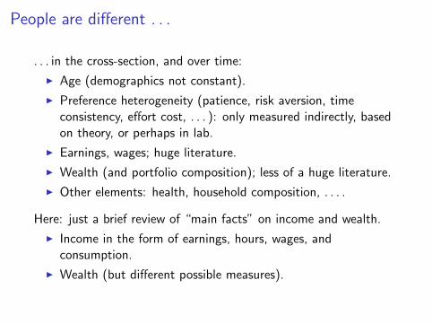
People are different . . .

. . . in the cross-section, and over time:

I Age (demographics not constant).

I Preference heterogeneity (patience, risk aversion, timeconsistency, effort cost, . . . ): only measured indirectly, basedon theory, or perhaps in lab.

I Earnings, wages; huge literature.

I Wealth (and portfolio composition); less of a huge literature.

I Other elements: health, household composition, . . . .

Here: just a brief review of “main facts” on income and wealth.

I Income in the form of earnings, hours, wages, andconsumption.

I Wealth (but different possible measures).

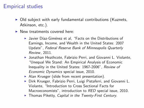
Empirical studies

I Old subject with early fundamental contributions (Kuznets,Atkinson, etc.).

I New treatments covered here:

I Javier Dıaz-Gimenez et al, “Facts on the Distributions ofEarnings, Income, and Wealth in the United States: 2007Update”, Federal Reserve Bank of Minneapolis QuarterlyReview , 2011.

I Jonathan Heathcote, Fabrizio Perri, and Giovanni L. Violante,“Unequal We Stand: An Empirical Analysis of EconomicInequality in the United States: 1967-2006”, Review ofEconomic Dynamics special issue, 2010.

I Alan Krueger (slide from recent presentation).I Dirk Krueger, Fabrizio Perri, Luigi Pistaferri, and Giovanni L.

Violante, “Introduction to Cross Sectional Facts forMacroeconomists”, introduction to RED special issue, 2010.

I Thomas Piketty, Capital in the Twenty-First Century.

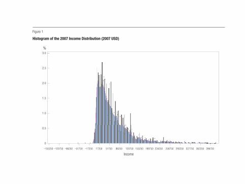
–155250 –120750 –86250 –51750 –17250 17250 51750 86250 120750 155250 189750 224250 258750 293250 327750 362250 396750

3.0

2.5

2.0

1.5

1.0

0.5

0

Figure 1

Histogram of the 2007 Income Distribution (2007 USD)

%

Income

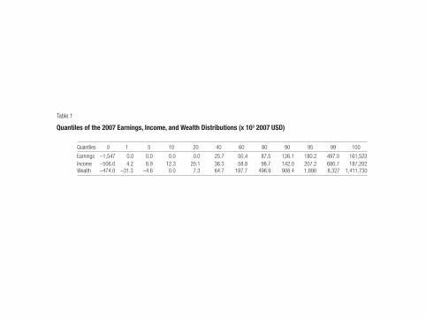
Table 1Table 1

Quantiles of the 2007 Earnings, Income, and Wealth Distributions (x 103 2007 USD)

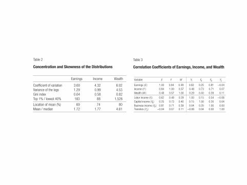
Table 3

Correlation Coefficients of Earnings, Income, and Wealth

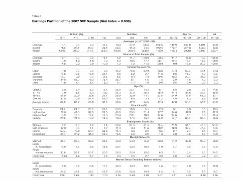
Table 4

Earnings Partition of the 2007 SCF Sample (Gini Index = 0.636)

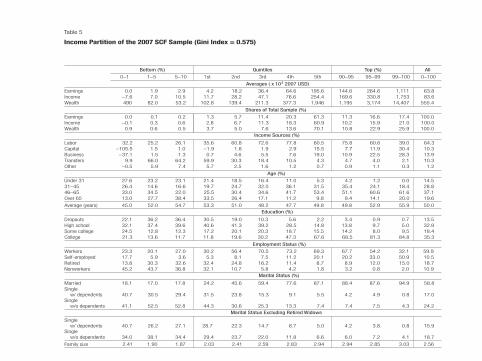
Table 5

Income Partition of the 2007 SCF Sample (Gini Index = 0.575)

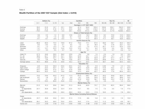
Table 6

Wealth Partition of the 2007 SCF Sample (Gini Index = 0.816)

A large majority of the household heads in this group (88 percent) have completed college. Many of them are self-employed (48 percent, which is more than four times the sample average), and almost all of them are

The earnings-rich are still rich along all three dimensions, but appreciably less so than the earnings-richest. Their average earnings, income, and wealth are about three times the sample averages. Their income sources are similar to the sample aver-ages. When compared with the earnings-richest, more

their income comes from labor and less from busi-ness and capital sources. The household heads are still

ing completed college. A very large share of them are

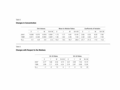
Table 8

Changes in Concentration

Table 9

Changes with Respect to the Medians

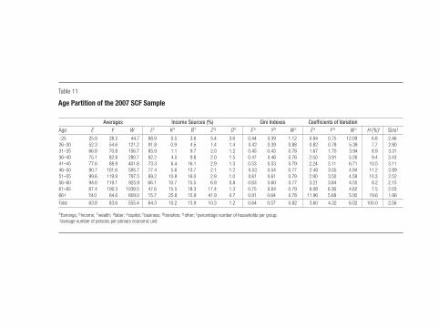
Table 11

Age Partition of the 2007 SCF Sample

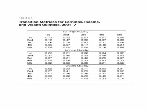
closer look at earnings mobility in Table 28, where we show the transition matrices of those in the 35–45 age

Table 27

Transition Matrices for Earnings, Income,

and Wealth Quintiles, 2001–7

1970 1975 1980 1985 1990 1995 2000 2005

0.2

0.25

0.3

0.35

0.4

0.45

Year

Variance of Log Hourly Wages

1970 1975 1980 1985 1990 1995 2000 2005

0.26

0.28

0.3

0.32

0.34

0.36

0.38

Gini Coefficient of Hourly Wages

Year

1970 1975 1980 1985 1990 1995 2000 20051.7

1.8

1.9

2

2.1

2.2

2.3

2.4

P50−P10 Ratio of Hourly Wages

Year

1970 1975 1980 1985 1990 1995 2000 20051.7

1.8

1.9

2

2.1

2.2

2.3

2.4

Year

P90−P50 Ratio of Hourly Wages

Men

Women

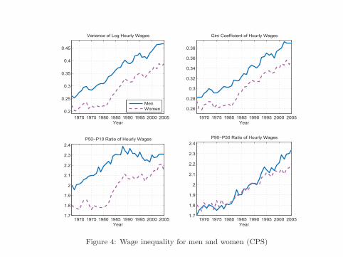
Figure 4: Wage inequality for men and women (CPS)

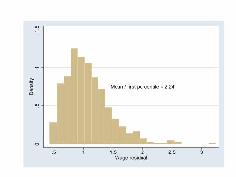
Mean / first percentile = 2.24

0.5

11.5

Density

.5 1 1.5 2 2.5 3Wage residual

1970 1975 1980 1985 1990 1995 2000 2005

0.15

0.2

0.25

0.3

0.35

0.4

0.45

0.5

Variance of Log Hourly Wages

Year

1970 1975 1980 1985 1990 1995 2000 20050

0.05

0.1

0.15

0.2

0.25

0.3

0.35

0.4Variance of Log Annual Hours

Year

1970 1975 1980 1985 1990 1995 2000 2005−0.17

−0.12

−0.07

−0.02

0.03

0.08

0.13

0.18

Correl. btw Log Hours and Log Wages

Year

1970 1975 1980 1985 1990 1995 2000 20050.4

0.45

0.5

0.55

0.6

0.65

0.7

0.75

0.8Variance of Log Annual Earnings

Year

Men

Women

Figure 6: Inequality in labor supply and earnings of men and women (CPS)

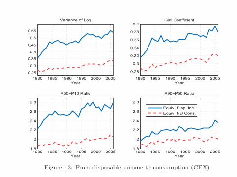
1980 1985 1990 1995 2000 2005

0.25

0.3

0.35

0.4

0.45

0.5

0.55

Variance of Log

Year

1980 1985 1990 1995 2000 2005

0.28

0.3

0.32

0.34

0.36

0.38

0.4Gini Coefficient

Year

1980 1985 1990 1995 2000 20051.8

2

2.2

2.4

2.6

2.8

P50−P10 Ratio

Year

1980 1985 1990 1995 2000 20051.8

2

2.2

2.4

2.6

2.8

P90−P50 Ratio

Year

Equiv. Disp. Inc.

Equiv. ND Cons.

Figure 13: From disposable income to consumption (CEX)

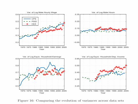
1970 1975 1980 1985 1990 1995 2000 2005

0.2

0.3

0.4

0.5

0.6

Var. of Log Male Hourly Wage

Year

1970 1975 1980 1985 1990 1995 2000 2005

−0.05

0.05

0.15

0.25

0.35Var. of Log Male Hours

Year

1970 1975 1980 1985 1990 1995 2000 2005

0.5

0.6

0.7

0.8

0.9Var. of Log Equiv. Household Earnings

Year

1970 1975 1980 1985 1990 1995 2000 2005

0.25

0.35

0.45

0.55

0.65Var. of Log Equiv. Household Disp. Income

Year

CPS

PSID

CEX

Figure 16: Comparing the evolution of variances across data sets

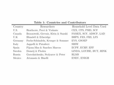
Table 1: Countries and Contributors

Country Researchers Household Level Data Used

U.S. Heathcote, Perri & Violante CEX, CPS, PSID, SCF

Canada Brzozowski, Gervais, Klein & Suzuki FAMEX, SCF, ADSCF, LAD

U.K Blundell & Etheridge BHPS, FES, FRS, LFS

Germany Fuchs-Schundeln, Krueger & Sommer EVS, GSOEP

Italy Jappelli & Pistaferri SHIW

Spain Pijoan-Mas & Sanchez Marcos ECPF, ECHP, EFF

Sweden Domeij & Floden LINDA, LOUISE, HUT, HINK

Russia Gorodnichenko, Stolyarov & Peter RLMS

Mexico Attanasio & Binelli ENEU, ENIGH

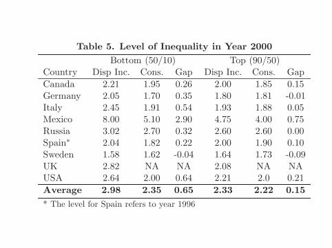
Table 5. Level of Inequality in Year 2000

Bottom (50/10) Top (90/50)Country Disp Inc. Cons. Gap Disp Inc. Cons. Gap

Canada 2.21 1.95 0.26 2.00 1.85 0.15Germany 2.05 1.70 0.35 1.80 1.81 -0.01Italy 2.45 1.91 0.54 1.93 1.88 0.05Mexico 8.00 5.10 2.90 4.75 4.00 0.75Russia 3.02 2.70 0.32 2.60 2.60 0.00Spain∗ 2.04 1.82 0.22 2.00 1.90 0.10Sweden 1.58 1.62 -0.04 1.64 1.73 -0.09UK 2.82 NA NA 2.08 NA NAUSA 2.64 2.00 0.64 2.21 2.0 0.21

Average 2.98 2.35 0.65 2.33 2.22 0.15

* The level for Spain refers to year 1996

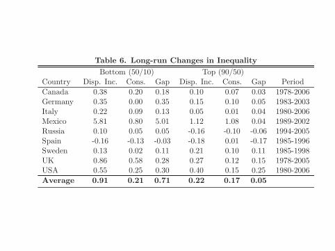
Table 6. Long-run Changes in Inequality

Bottom (50/10) Top (90/50)Country Disp. Inc. Cons. Gap Disp. Inc. Cons. Gap Period

Canada 0.38 0.20 0.18 0.10 0.07 0.03 1978-2006Germany 0.35 0.00 0.35 0.15 0.10 0.05 1983-2003Italy 0.22 0.09 0.13 0.05 0.01 0.04 1980-2006Mexico 5.81 0.80 5.01 1.12 1.08 0.04 1989-2002Russia 0.10 0.05 0.05 -0.16 -0.10 -0.06 1994-2005Spain -0.16 -0.13 -0.03 -0.18 0.01 -0.17 1985-1996Sweden 0.13 0.02 0.11 0.21 0.10 0.11 1985-1998UK 0.86 0.58 0.28 0.27 0.12 0.15 1978-2005USA 0.55 0.25 0.30 0.40 0.15 0.25 1980-2006

Average 0.91 0.21 0.71 0.22 0.17 0.05

Higher Income Inequality Associated with Lower Intergenerational Mobility

Denmark

Finland

France

GermanyJapan

New Zealand

Norway

Sweden

United Kingdom

United States

y = 2.2x - 0.27R² = 0.76

0.1

0.2

0.3

0.4

0.5

0.6

0.1

0.2

0.3

0.4

0.5

0.6

0.15 0.20 0.25 0.30 0.35 0.40

Inequality(1985 Gini Coefficient)

Intergenerational earnings elasticity

The Great Gatsby Curve

y = 2.2x - 0.27R² = 0.76

.

Source: Corak (2011), OECD, CEA estimates

g

14June 17, 2014

I C O

100%

90%

80%

70%

60%

50%

40%

30%

20%

10%

0%1810 1830 1850 1870 1890 1910 1930 1950 1970 1990 2010

Sh

are

of

top

dec

ile

or

per

cen

tile

in

to

tal

wea

lth

Top 10% wealth share:Europe

Top 10% wealth share:United States

Top 1% wealth share:Europe

Top 1% wealth share:United States

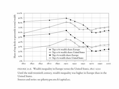
Figure 10.6. Wealth in e qual ity in Eu rope versus the United States, 1810– 2010

Until the mid- twentieth century, wealth in e qual ity was higher in Eu rope than in the United States.Sources and series: see piketty.pse.ens.fr/capital21c.

T S I

24%

22%

20%

18%

16%

14%

12%

10%

8%

6%

4%

2%

0%1910 1920 1930 1940 1950 1960 1970 1980 1990 2000 2010

Sh

are

of

top

per

cen

tile

in

to

tal

inco

me United States Britain

Canada Australia

Figure 9.2. Income in e qual ity in Anglo- Saxon countries, 1910– 2010

! e share of top percentile in total income rose since the 1970s in all Anglo- Saxon countries, but with di erent magnitudes.Sources and series: see piketty.pse.ens.fr/capital21c.

I L I

24%

22%

20%

18%

16%

14%

12%

10%

8%

6%

4%

2%

0%1910 1920 1930 1940 1950 1960 1970 1980 1990 2000 2010

Shar

e of

top

per

cen

tile

in t

otal

inco

me France Germany

Sweden Japan

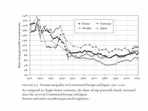
Figure 9.3. Income in e qual ity in Continental Eu rope and Japan, 1910– 2010

As compared to Anglo- Saxon countries, the share of top percentile barely increased since the 1970s in Continental Eu rope and Japan.Sources and series: see piketty.pse.ens.fr/capital21c.

T S I

24%

22%

20%

18%

16%

14%

12%

10%

8%

6%

4%

2%

0%1910 1920 1930 1940 1950 1960 1970 1980 1990 2000 2010

Shar

e of

top

per

cen

tile

in t

otal

inco

me France Denmark

SpainItaly

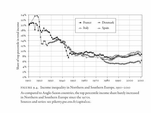
Figure 9.4. Income in e qual ity in Northern and Southern Eu rope, 1910– 2010

As compared to Anglo- Saxon countries, the top percentile income share barely increased in Northern and Southern Eu rope since the 1970s.Sources and series: see piketty.pse.ens.fr/capital21c.

I L I

28%

26%

24%

22%

20%

18%

16%

14%

12%

10%

8%

6%

4%

2%

0%

Shar

e of

top

per

cen

tile

in t

otal

inco

me

1910 1920 1930 1940 1950 1960 1970 1980 1990 2000 2010

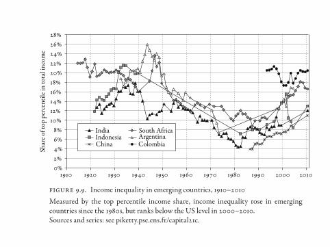
IndiaIndonesiaChina Colombia

ArgentinaSouth Africa

Figure 9.9. Income in e qual ity in emerging countries, 1910– 2010

Mea sured by the top percentile income share, income in e qual ity rose in emerging countries since the 1980s, but ranks below the US level in 2000– 2010.Sources and series: see piketty.pse.ens.fr/capital21c.

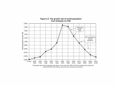
Figure 2.2. The growth rate of world population from Antiquity to 2100

400%

500%

600%

700%

800%

Ma

rke

t va

lue

of p

riva

te c

ap

ita

l (%

na

tio

na

l in

co

me

)

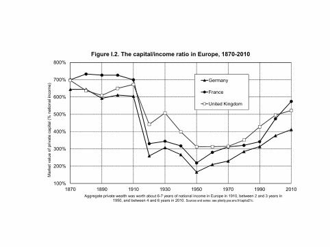
Germany

France

United Kingdom

100%

200%

300%

1870 1890 1910 1930 1950 1970 1990 2010

Ma

rke

t va

lue

of p

riva

te c

ap

ita

l (%

na

tio

na

l in

co

me

)

Aggregate private wealth was worth about 6-7 years of national income in Europe in 1910, between 2 and 3 years in 1950, and between 4 and 6 years in 2010.