Comparative Politics and Public Finance 1

Torsten PerssonIIES, Stockholm University; CEPR; NBER.

Gerard RolandECARE, University of Brussels; CEPR.

Guido TabelliniBocconi University; CEPR; CES-Ifo

Abstract

We propose a model with micropolitical foundations to contrast different politi-cal regimes. Compared to a parliamentary regime, the institutions of a presidential-congressional regime produce less incentives for legislative cohesion, but more separa-tion of powers. These differences are reflected in the size and composition of governmentspending. A parliamentary regime has redistribution towards a majority, less underpro-vision of public goods, more rents to politicians, whereas a presidential-congressionalregime has redistribution towards powerful minorities, more underprovision of publicgoods, but less rents to politicians. The size of government is smaller under a presi-dential regime. This last prediction is consistent with cross-country data.

JEL classification: H00, D72, D78.

Keywords: political economics, comparative politics, public finance, separation ofpowers, legislative cohesion, electoral accountability.

2

1. Introduction

The level and composition of government spending displays enormous variation, bothover time and across countries. In a sample of 17 industrialized democracies, averagegovernment expenditure as a fraction of GDP grew from about 12% in 1913 to about45% in 1990; but the 1990 level ranged from about 32% in Japan to about 59 % inSweden.2 Furthermore, while the average GDP share of transfers and subsidies grewvery rapidly, from about 8 % in 1960 to about 23 % in 1990, government consumptiononly increased from about 12 % to 17 %, whereas public investment was almost flat; thecross-country variation is also considerable in these dimensions. In a broader sampleof 54 democracies, the cross-country variation in the size and scope of government iseven greater (see Section 6, below).It is fair to say that the economics profession has failed to convincingly explain

these first-order differences. Research in traditional public finance does not ask thequestion, since its policy analysis is mostly normative and abstracts from the underly-ing political institutions. Research in traditional public choice and, more recently, inpolitical economics does attempt to explain actual policy outcomes. So far, however,it has only come up with fragmented explanations for the growth, size, and scope ofgovernment.3

In our view, a successful positive theory of public finance in a democracy shouldrest on appropriate micro-political foundations, analyzing the incentives for collectivepolicy decisions entailed by different political regimes. In this paper, we try to takea step towards building such micro-political foundations. More specifically, we tryto demonstrate how key differences between real-world political regimes can createsystematic differences in collective decisions on taxation, redistribution, public goodprovision, and rent-seeking.We build on three basic assumptions: (1) No benevolent actors: all agents, includ-

ing politicians, are motivated by their own selfish objectives. (2) No direct democracy:citizens delegate policy decisions to their political agents. Although delegation shouldideally be endogenously derived, we take the prevalence of representative democracyas a starting point, which reflects either specialization in acquiring competence andinformation, or the practical difficulty in using direct democracy in all policy decisions.(3) No outside enforcement: political candidates cannot commit to policy platformsahead of the elections. Elected political offices, whether executive or legislative, carryimportant powers that are always partly–sometimes even greatly–unchecked. Unbi-ased enforcement of electoral promises is therefore not feasible and not observed in thereal world. Together with non-benevolence and delegation, no enforcement implies anagency problem between voters and their representatives.These three assumptions appear in many existing positive models of policy making.

But the three are seldom explicitly combined, and their full implications are rarelystudied. The traditional public choice school comes close in its emphasis of the agencyproblem (see, for instance, Brennan and Buchanan (1980)). It is not very formal inspecifying the underlying assumptions, however, and sometimes neglects the role ofelections and other political institutions in disciplining political agents. Moral hazardmodels of elections (Barro (1973) and Ferejohn (1986)), on the other hand, study how

3

elections may discipline political representatives, but they do not study different insti-tutions and impose restrictions on available policies. Median-voter models sometimesrefer to policy choice under direct democracy (Meltzer and Richard (1981)). A moreconvincing interpretation of these models, however, is that they capture the outcomeof electoral competition between two office-motivated politicians who can commit tostate contingent electoral promises (Downs (1957)), thus implicitly violating the as-sumption of no outside enforcement. Likewise, models of lobbying and electoral com-petition among selfish candidates under probabilistic voting assume that some politi-cal actors–lobbies, politicians, or both–can undertake explicit commitments (Gross-man and Helpman (1994), (1996), Lindbeck and Weibull (1987), Dixit and Londregan(1996)). Models of partisan politics remove the commitment assumption, but typicallyconsider ideological policymakers with altruistic objective functions (Alesina (1988),Alesina and Rosenthal (1996)). Recent models of representative democracy (Besleyand Coate (1997)) essentially rely on the same three basic assumptions, but imposerestrictions on what policy can do, thereby ruling out the agency problem.We build a model of public spending under alternative political institutions that

incorporates the three basic assumptions. In our model, the political process mustdetermine a level of taxation, as well as an allocation of tax revenues to public goods,redistribution among voters, and rents for politicians. Thus three conflicts of interestemerge: policy-makers may abuse their power in office and capture public funds fortheir own benefit at the voters’ expense; different groups of voters disagree on theallocation of tax revenues; and the political representatives, each pursuing her owncareer and personal interests, disagree over the distribution of current and future rents.These conflicts of interest are resolved in different ways under different constitu-

tions. The reason is that, under our basic assumptions,a political constitution is likean incomplete contract. A constitution can only specify an allocation of decision-making authority to specific groups or individuals: who makes policy proposals, whocan approve, amend, or veto them, and who appoints the representatives exercisingthis authority.4 Given the three-dimensional conflict in our policy problem, the out-come hinges on how and by whom these authorities are exercised. We illustrate thisgeneral point by contrasting two main types of democracies: presidential-congressionalvs. parliamentary regimes. In doing so, we concentrate on two important features ofthese regimes: separation of powers and legislative cohesion, and ask how they shapepublic finance outcomes.Separation of powers in some form is a feature of all modern democracies. Since

Locke, Montesqieu and the founding fathers of the American constitution, it is commonto consider such separation as limiting abuse and increasing accountability of electedpolicy-makers. Persson, Roland and Tabellini (1997) show formally that conflicts ofinterest between different politicians can indeed be exploited by the voters in order toreduce the agency problem. But this requires that the constitution allocates the rightsto propose and veto legislation across different representatives so as to create the rightchecks and balances.Legislative cohesion refers to disciplined voting by members of a governing coalition.

The pioneering work of Diermeier and Feddersen (1998) shows that legislative cohesionarises when it is costly for a majority coalition to break up, for instance because it

4

loses valuable agenda-setting powers associated with participation in the coalition. Theextent to which a political regime displays legislative cohesion thus largely depends onthe rights laid down by the constitution concerning the formation and dissolution ofgovernments.A presidential-congressional regime of the US type has more separation of powers

but less legislative cohesion than a parliamentary regime of the European type. Directelection of both the executive and the legislature makes each branch of governmentdirectly accountable to the voters. This diminishes the opportunities for collusion be-tween the branches of government and can even create outright conflicts between them,as in the case of “divided government”. Moreover, the proposal powers over legislationtypically reside with powerful congressional committees, and different committees holdpower over different policy dimensions. Hence powers are separated not only betweenexecutive and legislature, but also within the legislature. As a result, legislative ma-jorities often change from issue to issue. In particular, no stable congressional majorityis needed to support the executive, as the latter is directly elected for an entire electionperiod and cannot be voted down by Congress.In a parliamentary regime, by contrast, the executive is only indirectly appointed by

the voters and instead derives its power from the support by a majority coalition in thelegislature. In addition, the agenda-setting powers over legislation are typically associ-ated with ministerial portfolios, and the policy initiative thus belongs to the governmentcoalition as long as it has the confidence of a majority in parliament. As a result, par-liamentary regimes entail less separation of powers than congressional regimes, bothbetween executive and legislature and between different legislators. Moreover, govern-ment crises can erupt during an election period, due to the rights of initiating votes ofconfidence or non-confidence, of dissolving the government, or calling early elections.As Huber (1996) demonstrates, the power to associate a vote on a bill with a vote ofconfidence reduces the bargaining power of the coalition partners who fear the negativeconsequences of a government crisis. The risk of losing valuable agenda-setting powersafter a government crisis then gives a governing coalition strong incentives to form astable legislative majority that does not shift from issue to issue, as shown by Diermeierand Feddersen (1998). Note that this argument goes beyond party discipline: cohe-sion between parties supporting coalition governments is typically much higher thancohesion within parties in the US congress.5

Our goal is to compare alternative political constitutions, representing the key fea-tures of each regime with a very stylized model of the policy process. In our modeling,we build on several earlier contributions. Specifically, the public-finance instrumentsare chosen in a sequence of simple legislative-bargaining games, in the style of Baron andFerejohn (1989); the extensive form of each game represents a specific constitutionalprocedure. This legislative bargaining is embedded in the same infinitely repeated elec-toral framework, where voters in each different district hold their legislator accountablefor past performance in first-past-the-post elections, as in Ferejohn (1986). Separationof powers in presidential regimes is modeled as in Persson, Roland and Tabellini (1997),namely as an assignment of very sharp proposal rights over different policy dimensionsto different politicians. Legislative cohesion in our model of a parliamentary regimeis obtained through a simplified version of the model formulated in Diermeier and

5

Feddersen (1998), by assuming that the agenda-setting powers are reallocated, if thelegislative coalition breaks down.6

Our results suggest that the two political regimes are associated with very differentpolicy outcomes. Separation of powers in the congressional regime produces a smallergovernment, with less waste, less redistribution, but also inefficiently low spending onpublic goods. Intuitively, separation of powers enables the voters to discipline thepoliticians, and this reduces waste and moderates the tax burden. The sharp conflictof interest among politicians and voters, however, prevents them from internalizing allbenefits of public good provision. Legislative cohesion in the parliamentary regime,on the other hand, leads to a larger government, with more taxation and more waste,but also more spending on public goods and redistribution benefiting a broader groupof voters. Intuitively, there is now more scope for collusion among politicians, whichincreases waste and taxation. But policy aims to please a majority group of voterswhich increases public good provision, calls for a more equal redistribution, and makesthe majority support a high level of taxation.These results could help explain some of the observed differences in patterns of

spending and taxation among modern democracies. The evidence in Persson andTabellini (1999b) suggests that, everything else equal, the size of government in presidential-congressional regimes is smaller than in parliamentary regimes by about 10% of GDP.There is less evidence of significant differences in the composition of public spend-ing across regimes, but distinguishing empirically global from local public goods andredistribution is more difficult and necessitates further research.>From a normative point of view, our results point to a trade-off in institution

design. A well-functioning presidential regime performs better in terms of accountabil-ity, because it can cope well with the agency problem between voters and politicians.But a parliamentary regime is better for public good provision, because it solves theconflict between groups of voters more effectively.In the following, we first introduce the notation and present the basic policy prob-

lem (Section 2). We then study the political equilibrium in a “simple legislature”which has neither separation of powers nor legislative cohesion (Section 3). After thesepreliminaries, we derive our main results, first for a presidential-congressional regimewith separation of powers (Section 4), then for a parliamentary regime with legislativecohesion (Section 5). We then briefly consider the evidence (Section 6). Last (Section7) we discuss prospective extensions.

2. A basic model of public finance

Consider a society with three distinct groups of citizens, denoted by i = 1, 2, 3. Weshall consider these groups as distinguished by their geographical location. Otherinterpretations are possible, but less natural. Three groups is the minimum numberfor looking at interesting legislative bargaining under majority rule, but we could carryout the analysis with more than three groups at the cost of more cumbersome algebra.Each group has a large number of identical members: formally we assume that eachgroup has a continuum of voters with unit mass. Time is measured discretely: a typicaltime period is denoted by t. We consider an infinite horizon.

6

Preferences of a member of group i in an arbitrary starting period j are given by:

uij =∞Xt=j

δ(t−j)U i(qt), (2.1)

where δ < 1 is a discount factor, qt is a vector of policies at t (to be defined below),and U i is the per period utility function. The latter is assumed to be quasi-linear inthe consumption of private and public goods:

U i(qt) = cit +H(gt) = 1− τ t + rit +H(gt), (2.2)

where τ t is a common tax rate, rit is a transfer payment to group i, and gt is thesupply of Samuelsonian public goods evaluated by all voters with the same concaveand monotonically increasing function H(gt).We assume that these goods are valuableto citizens, in the sense that Hg(0) > 1.We define the public policy vector q as:

qt = [τ t, gt, {rit}, {slt}],where all components are constrained to be non-negative. In an economic model,it would only be necessary to distinguish the net government transfer to each grouprit−τ t. But in the political models to be considered below, it is of crucial importance todistinguish the two components, particularly when different politicians have agenda-setting rights over taxes and spending. The component {slt} captures the possiblediversion of resources by politicians. As discussed in Persson, Roland and Tabellini(1997), we can think of {slt} as the financing of political parties, as outright diversion,or as an allocation of resources benefiting the private agenda of the legislators butnot the citizens. These diversions benefit some politicians more than others: thus, sltdenotes the diversion benefiting legislator l, but no other legislator. From the viewpointof the citizens, these rents for the legislators represent pure waste. It is natural tothink that this diversion takes place in connection with public goods production, gt.7

This association between resource diversion and public good provision will play a rolebelow, with reference to the allocation of agenda-setting rights over the various policyinstruments.The public policy vector in period t must satisfy the government budget constraint:

3τ t =Xi

rit +Xl

slt + gt ≡ rt + st + gt, (2.3)

where rt and st in the rightmost expression, denote aggregate redistributive expendi-tures and aggregate waste.To make the public finance problem more interesting, we could extend the model

with some private choices distorted by taxation. This would make our results quantita-tively, but not qualitatively, different. Note, however, that the micro-political probleminherent in this formulation is quite general: it involves activities benefiting every cit-izen (gt and −τ t) benefiting some citizens but not others ({rit}), and benefiting somepoliticians but not others ({slt}). As we shall see, the trade-off on each different marginof policy choice plays a non-trivial role in shaping the results.

7

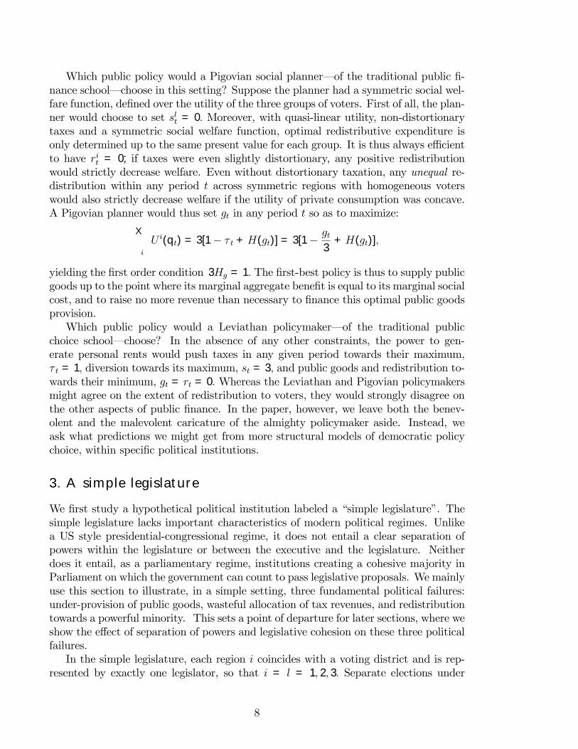
Which public policy would a Pigovian social planner–of the traditional public fi-nance school–choose in this setting? Suppose the planner had a symmetric social wel-fare function, defined over the utility of the three groups of voters. First of all, the plan-ner would choose to set slt = 0. Moreover, with quasi-linear utility, non-distortionarytaxes and a symmetric social welfare function, optimal redistributive expenditure isonly determined up to the same present value for each group. It is thus always efficientto have rit = 0; if taxes were even slightly distortionary, any positive redistributionwould strictly decrease welfare. Even without distortionary taxation, any unequal re-distribution within any period t across symmetric regions with homogeneous voterswould also strictly decrease welfare if the utility of private consumption was concave.A Pigovian planner would thus set gt in any period t so as to maximize:X

i

U i(qt) = 3[1− τ t +H(gt)] = 3[1− gt3

+H(gt)],

yielding the first order condition 3Hg = 1. The first-best policy is thus to supply publicgoods up to the point where its marginal aggregate benefit is equal to its marginal socialcost, and to raise no more revenue than necessary to finance this optimal public goodsprovision.Which public policy would a Leviathan policymaker–of the traditional public

choice school–choose? In the absence of any other constraints, the power to gen-erate personal rents would push taxes in any given period towards their maximum,τ t = 1, diversion towards its maximum, st = 3, and public goods and redistribution to-wards their minimum, gt = rt = 0. Whereas the Leviathan and Pigovian policymakersmight agree on the extent of redistribution to voters, they would strongly disagree onthe other aspects of public finance. In the paper, however, we leave both the benev-olent and the malevolent caricature of the almighty policymaker aside. Instead, weask what predictions we might get from more structural models of democratic policychoice, within specific political institutions.

3. A simple legislature

We first study a hypothetical political institution labeled a “simple legislature”. Thesimple legislature lacks important characteristics of modern political regimes. Unlikea US style presidential-congressional regime, it does not entail a clear separation ofpowers within the legislature or between the executive and the legislature. Neitherdoes it entail, as a parliamentary regime, institutions creating a cohesive majority inParliament on which the government can count to pass legislative proposals. We mainlyuse this section to illustrate, in a simple setting, three fundamental political failures:under-provision of public goods, wasteful allocation of tax revenues, and redistributiontowards a powerful minority. This sets a point of departure for later sections, where weshow the effect of separation of powers and legislative cohesion on these three politicalfailures.In the simple legislature, each region i coincides with a voting district and is rep-

resented by exactly one legislator, so that i = l = 1, 2, 3. Separate elections under

8

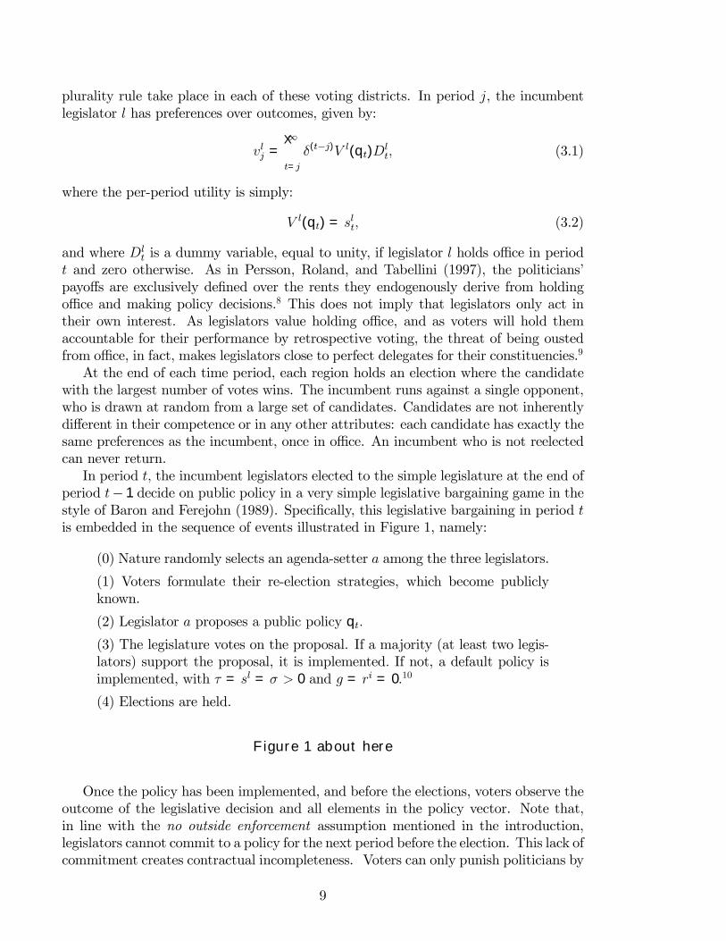
plurality rule take place in each of these voting districts. In period j, the incumbentlegislator l has preferences over outcomes, given by:

vlj =∞Xt=j

δ(t−j)V l(qt)Dlt, (3.1)

where the per-period utility is simply:

V l(qt) = slt, (3.2)

and where Dlt is a dummy variable, equal to unity, if legislator l holds office in period

t and zero otherwise. As in Persson, Roland, and Tabellini (1997), the politicians’payoffs are exclusively defined over the rents they endogenously derive from holdingoffice and making policy decisions.8 This does not imply that legislators only act intheir own interest. As legislators value holding office, and as voters will hold themaccountable for their performance by retrospective voting, the threat of being oustedfrom office, in fact, makes legislators close to perfect delegates for their constituencies.9

At the end of each time period, each region holds an election where the candidatewith the largest number of votes wins. The incumbent runs against a single opponent,who is drawn at random from a large set of candidates. Candidates are not inherentlydifferent in their competence or in any other attributes: each candidate has exactly thesame preferences as the incumbent, once in office. An incumbent who is not reelectedcan never return.In period t, the incumbent legislators elected to the simple legislature at the end of

period t− 1 decide on public policy in a very simple legislative bargaining game in thestyle of Baron and Ferejohn (1989). Specifically, this legislative bargaining in period tis embedded in the sequence of events illustrated in Figure 1, namely:

(0) Nature randomly selects an agenda-setter a among the three legislators.

(1) Voters formulate their re-election strategies, which become publiclyknown.

(2) Legislator a proposes a public policy qt.

(3) The legislature votes on the proposal. If a majority (at least two legis-lators) support the proposal, it is implemented. If not, a default policy isimplemented, with τ = sl = σ > 0 and g = ri = 0.10

(4) Elections are held.

Figure 1 about here

Once the policy has been implemented, and before the elections, voters observe theoutcome of the legislative decision and all elements in the policy vector. Note that,in line with the no outside enforcement assumption mentioned in the introduction,legislators cannot commit to a policy for the next period before the election. This lack ofcommitment creates contractual incompleteness. Voters can only punish politicians by

9

not reelecting them. The discretionary powers enjoyed by politicians between elections,however, makes it impossible for voters to insist on having slt = 0 for all l in equilibrium.As shown by Persson and Tabellini (1999a), if legislators could commit to a policybefore elections, electoral competition between the incumbent and the opponent ineach district would force them to set slt = 0. Thus, the rents extracted by politiciansin equilibrium are a direct result of the contractual incompleteness of the politicalconstitution.11

Given the infinite-horizon, there are many sequentially rational equilibria. Through-out the paper, we restrict our attention to equilibria where voters from the same con-stituency coordinate their strategies, but where voters across constituencies do notcooperate. Cooperation across constituencies with opposing interests on redistributionis not supported by the institutions analyzed and would only be supported by reputa-tional concerns ignored by us. Coordination inside a constituency is more reasonableas all these voters are identical. Such coordination could be supported by the exis-tence of alternative candidates campaigning on the policy that is in the best interest ofthe constituency. Throughout the paper, we also assume that all players (voters andpoliticians) are restricted to using strategies which condition their actions in period ton observable pay-off relevant information in period t only, and not on outcomes in anyearlier period. This is a reasonable restriction if we assume that voters cannot committo intertemporal reelection rules across periods. The restriction will effectively makethe equilibrium outcome stationary, and we drop time subscripts when there is no riskof confusion.We assume that voters in each district adopt simple retrospective voting rules,

conditional on their representative having been the agenda setter in period t or not.Since we assume that voters in each district coordinate on the voting rule, this impliesthat:

Dlt+1 = 1

if U i(qt) ≥ bit, i = l

for i = a and i 6= a at t. Finally, we assume that voters in all regions simultaneouslyset their “reservation utilities” bit in a utility-maximizing fashion.

12 While voters coop-erate within districts, they thus play Nash against all other districts; see the definitionof equilibrium below. The vector of these reservation utilities, bt, is thus known topoliticians when the policy proposal is made, and it is not altered by the voters inthe course of period t. Due to this feature, legislators will act in the interest of theirconstituencies. Allowing voters to condition directly on the policy instruments or onthe vote of the politicians would not change any of the results.Our assumption about the time when voters formulate their strategies deserves

some discussion. The timing means that the voters form their expectations and theirdemands on politicians once they know the institutional role of their representative atthe beginning of the policy formation process. That is, voters want to hold their rep-resentative accountable for her deeds in the course of the legislative process. Allowingvoters to re-optimize just before the election date would not change the results: asdiscussed below, the voting rule is ex-post optimal for the voters, since the incumbentand the opponent are identical in the eyes of the voters. Under a different timing,

10

however, there would be many other equilibria, besides the one discussed here. Thus,our timing assumption really amounts to a selection criterion: among the possible equi-libria emerging if voters do not commit to a voting rule, we select the only one thatsurvives under the timing spelled out above. If legislators and candidates were inher-ently different in their competence or other attributes, however, the timing assumptionwould be more critical, since the equilibrium voting rule would no longer be ex-postoptimal.13

An equilibrium of this game is defined as follows (the L superscript stands for thesimple Legislature):

Definition 1. An equilibrium of the simple legislature is a vector of policies qLt (bt)and a vector of reservation utilities bLt , such that in any period t, when all playerstake as given the equilibrium outcomes of periods t+ k, k ≥ 1:

(I) for any given bt, at least one legislator i 6= a weakly prefers qLt (bt) to the defaultoutcome;

(II) for any given bt, the agenda-setting legislator a prefers qLt (bt) to any otherpolicy satisfying (I);

(III) The reservation utilities biLt are optimal for the voters in each district i, takinginto account that policies in the current period are set according to qLt (bt) and takingas given the reservation utilities in other regions b−iLt and the identity of the agendasetter.

A unique and stationary equilibrium satisfies these conditions. Its properties aresummarized in the following proposition:

Proposition 1. In the equilibrium of the simple legislature:τL = 1;sL = 3 (1−δ)

1−δ/3;

gL = Min( bg, 2δ1−δ/3), where bg is such that Hg(bg) = 1 > 1/3;

raL = 2δ1−δ/3 − gL ≥ 0, riL = 0 for i 6= a;

baL = H(gL)− gL + 2δ(1−δ/3)

, biL = H(gL) for i 6= a.All politicians are re-elected.

Thus, in equilibrium taxes are maximal, public goods are underprovided relative tothe social optimum, some redistribution goes to a minority of voters (unless the publicgood is very valuable, in which case there is no redistribution at all), and the legislatorsappropriate positive rents from office.To understand how the model works, it is useful to prove this proposition in steps.

Consider districts m,n 6= a. We start with the following:

Lemma 1. In equilibrium, rm = rn = 0.

Proof. Note that any equilibrium entails a minimum winning coalition: that is,the equilibrium proposal is only approved by one other legislator besides the agendasetter. To get the support of the third legislator, the agenda setter would have to spendresources either on her or her district. But these resources are better used to increase

11

sa. Hence, if legislator n, say, is excluded from the winning coalition, then sn = rn = 0.By the same logic, the district included in the winning coalition is the one whose voteis the cheapest to buy. As all legislators have the same default payoffs, which districtis cheapest to buy only depends on the reservation utilities, bn and bm, demandedby the voters. Realizing this, the voters in districts m and n have an incentive tounderbid each other up to the point where rm = rn = 0, that is up to the point wherebm = bn = 1− τ +H(g) . QED.In other words, the voters become engaged in a “Bertrand competition” game for

the redistributive favors of the agenda setter. The utility of voters in district m isdiscontinuous in the reservation value bm, at the point where bm = bn, unless rm = 0.The same argument holds for voters in n. Hence the only equilibrium is at the cornerwhere rm = rn = 0.Next, defineW as the expected equilibrium continuation value for each legislator at

the start of each period, before nature has selected the agenda setter. Then we have:

Lemma 2. In equilibrium, s ≥ 3−2δW and all legislators are reappointed.

Proof. Consider the optimal behavior of the agenda setter, and let m be the otherlegislator supporting her proposal. Then, if a seeks reappointment, she will never offermore to m than:

sm = σ − δW, (3.3)

as this is what would leave m indifferent between voting yes and being reappointed, orvoting no, getting the default payoff σ and then losing the election.14

Suppose instead a does not seek reappointment, and makes a proposal that wouldlead to a loss of office for all legislators, under the given voting rules. In this case, shehas to offer at least σ to m to win approval of her proposal. Because she does not careabout pleasing her voters, the agenda setter can appropriate all available resources,setting g = r = 0 and τ = 1. Thus, a will seek reappointment if and only if:

sa + δW ≥ 3− σ. (3.4)

The left-hand side of (3.4) denotes the life-time utility of the agenda setter if she makesa proposal consistent with reappointment, under the given voting rule. The right-handside is her maximal payoff, given that she does not seek reappointment and has to payσ to m.By (3.3) and (3.4), legislators a and m will implement a policy leading to their

reappointment if and only if:

s = sm + sa ≥ 3− 2δW. (3.5)

The optimal voting rule can never be more demanding: if the legislators were inducedto forgo reappointment, they would appropriate all resources and leave the voters withlow utility. Hence, the optimal voting rule must satisfy (3.5), and both the agendasetter and the legislator supporting the proposal are reelected. The reservation utilityof voters in districts m and n is the same, as both districts receive zero transfers (byLemma 1). As these voters pay the same τ , and enjoy the same level of g, legislator nwill also be re-elected. QED.

12

Note that (3.5) is an incentive compatibility condition on the overall diversion ofresources. Note also that legislator a is the “residual claimant” on resources in periodt for given reelection strategies. It is thus optimal for her, not only to minimize thepayment to legislator m, but also to satisfy the reelection constraints of voters indistricts a and m with equality, appropriating any remaining resources for herself. Ifconsistent with her own reelection, she would thus like to set τ = 1.We are now ready to prove Proposition 1.

Proof of Proposition 1. Consider legislator a. As ra = r by Lemma 1, thepolicy maximizing the utility of voters in district a is the solution to:

Max [r + 1− τ +H(g)] ,

subject to the government budget constraint, (2.3), and the incentive constraint onlegislators a and m, (3.5). Combining (2.3) and (3.5), these constraints can be writtenas:

3(τ − 1) + 2δW ≥ r + g. (3.6)

The solution to this optimization problem implies: τ = 1, g = Min[H−1g (1), 2δW ],

r = 2δW − g, s = 3 − 2δW. Finally, by Lemma 2, all legislators are reappointed inequilibrium. We thus have:

W =s

3+ δW. (3.7)

Solving for W yields W = 11−δ/3 . Inserting the result in the expressions above

yields the equilibrium policies of Proposition 1. Inserting these policies in the voters’utility functions yields the equilibrium reservation utilities. By requiring the votingstrategies to maximize the utility of the representative voter in each district in anyperiod, we are guaranteeing that the equilibrium is sequentially rational. As voterssimultaneously choose their reelection strategies, no voter has any incentive to changeher vote, given the optimal behavior by other voters and of legislators, if she considersherself pivotal.15QED.This outcome is related to an equilibrium in the last section of Ferejohn (1986),

where a single policymaker gets away with massive rents when voters directly competefor her favors. In the simple legislature considered here, voters compete across, butnot within, districts, as redistribution only takes place across districts by assumption.Therefore, the voters in the agenda setter’s region can still discipline the agenda setterand keep rents to a minimum. This is done by adopting a reelection rule that keepspoliticians indifferent between diverting as much as possible today but losing office,and diverting a small amount only today but holding on to office and continuing toreap rents in the future.If r > 0, voters in region a obtain net redistribution to their district at the expense

of voters in other districts. Therefore, they prefer their representative to set taxes attheir maximum: τ = 1. There is an underprovision of public goods since the agendasetter effectively sets policy so as to maximize the utility of voters in district a only.She therefore trades off redistribution to region a and public goods provision one forone–and hence sets Hg(g) = 1.

13

Note also that the interests of voters in district a and their legislator are alignedin some dimensions, but not in others. Both want maximal taxes. But both thevoters and the legislator want to keep the revenue to themselves: voters wishing toexpand ra and the legislator wishing to expand sa. Holding their legislator accountablefor performance, the voters can limit the waste as long as they respect the incentiveconstraint (3.6).This simple model illustrates a form of legislation that Jefferson called “elective

despotism” in his Notes on North Virginia ( cited by Madison in Federalist PaperXLVIII, p. 310):

“All the powers of government, legislative, executive, and judiciary, result tothe legislative body. The concentrating these in the same hands is preciselythe definition of despotic government. It will be no alleviation that thesepowers will be exercised by a plurality of hands, and not by a single one.One hundred and seventy-three despots would surely be as oppressive as one(...) An elective despotism is not what we fought for”.

In our model, only the voters from one of three regions can secure redistributiontowards their region, whereas the other voters get nothing. Voters of the non-agenda-setting regions cannot discipline their representatives to ask for more equitable redis-tribution, because they compete with each other to be included in the majority.In summary, this simple legislative model displays three “political failures”, each be-

ing defined as a departure from the socially optimal policy: some spending is wasteful(sL > 0); public goods are underprovided (gL < H−1

g (1/3)); and a politically pow-erful minority receives any equilibrium redistribution (raL ≥ 0). We now ask whatform these three political failures take under alternative–and more realistic–politicalconstitutions.

4. A presidential-congressional regime

In this section, we modify the previous model by introducing separation of proposalpowers within the legislature. By giving different legislators sharp agenda-setting rightsover different dimensions of policy, we can approximate the agenda-setting powers ofthe powerful standing committees in legislatures, such as the US congress. Decisions aremade sequentially on different policy dimensions, subject to a budget constraint, wherelater proposals are bound by decisions taken at an earlier stage. That is, Congress votesdirectly on each separate proposal. This procedure with different agenda setters leadsto separation of powers. The reason is that the agenda setter is a different politicianat each stage, accountable to a different group of voters. The political regime thereforecaptures some features of a presidential regime, like that of the US. The direct electionof the executive makes it unnecessary to form a stable majority to support a cabinet.Nothing then constrains the kind of coalitions that can be formed. In other words,incentives for legislative cohesion–the focus of the next section–are absent.For simplicity, in the model of this section, we mainly focus on two-stage decision

making inside Congress, with one stage for taxes, the other stage for allocation of

14

spending. At the end, we comment on how the results would change with separationof agenda-setting powers between the President and Congress and with separation ofproposal powers in the allocation of expenditures as well.Voters use the same kind of retrospective voting rules for their congressional rep-

resentatives as in (3.3), conditioning their reservation utilities on whether their repre-sentative is the agenda setter for the allocation of spending, i = ag, for taxes, i = aτ ,or for neither (i = n):

Dlt+1 = 1 (4.1)

if U i(qt) ≥ bi, i = l at t

The extensive form of the game in a typical period is illustrated in Figure 2. Specifically,we consider the following sequence of events:

(0) Nature randomly selects two different agenda setters among the incum-bent legislators, one for taxes and one for the allocation of public spending,aτ , and ag, respectively.

(1) Voters set reservation utilities for their voting rule, bi.

(2) aτ proposes a tax rate, τ .

(3) Congress votes. If at least two legislators are in favor of the proposal,the policy is implemented. Otherwise, a default tax rate τ = σ < 1 isenacted.

(4) ag proposes [g, {si}, {ri}], subject to the budget constraint: r+ s+g ≤3τ .

(5) Congress votes. If at least two legislators are in favor, the policy isimplemented. Otherwise, a default policy, with g = 0, ri = 0 , si = τ , isput in place.

(6) Elections are held.

Figure 2 about here

Note that the sequentially of decisions matters also outside of equilibrium. What-ever the outcome of the decision over taxes, that outcome is binding at subsequentstages, even if there is disagreement over the allocation of spending (see the defaultoutcome at stage (5)). This feature is critical for the result stated below. At stage (4)legislator ag attempts to form the coalition that is best for her. In case ag is indifferentbetween the other two, we assume they have the same probability of being includedin the winning coalition. The reason why we must spell out how coalitions are formedin the last stage of the legislative bargaining is that legislators are forward-looking.Hence, their behavior in stages (2) and (3) depends on their expectations of what hap-pens in subsequent stages - in particular on whether they expect to be part of the

15

winning coalitions later on. Below, we discuss the consequences of making alternativeassumptions about coalition formation.An equilibrium is defined as in the previous section, except that here, the optimality

conditions for policy proposals and for voting by the legislators must hold at each nodeof the game, for any given voting rules and decisions at earlier nodes in the same period,and taking equilibrium behavior at subsequent nodes of the same period into account.A precise definition is stated in the Appendix.The stationary equilibrium is unique.16 Its features are summarized in the following

(a C super-script stands for Presidential-Congressional regime):

Proposition 2. In the equilibrium of the presidential-congressional regime:

τC = 1−δ/31+2δ/3

< 1;

sC = 3 (1−δ)1+2δ/3

< sL;

gC = Min(bg, 2δ1+2δ/3

) ≤ gL, where bg is such that Hg(bg) = 1 > 1/3;

raC = 2δ1+2δ/3

− gC ≤ raL, riC = 0 for i 6= a;

baC = H(gC)− gC + 2δ(1+2δ/3)

, biC = H(gC) for i 6= a.

All politicians are reelected.

Proof. To prove this proposition, begin at stages (4) and (5) of the game. Here,the agenda setter ag takes τ as given. By the same argument as in the proof of Lemma2, incentive compatibility implies that she must get at least:

sag ≥ 2τ − δW (4.2)

and that she offers:

smg = τ − δW (4.3)

to her junior coalition partner in order to win approval. Thus, total diversion inequilibrium must be at least:

s ≥ 3τ − 2δW. (4.4)

Together with the budget constraint, (4.4) implies that voters cannot get more publicgoods and redistribution than:

r + g ≤ 2δW. (4.5)

Repeating the same steps as in the proof of Lemma 1, one can show that, inequilibrium, all r (if any) is distributed to the district of ag. That is, ra = r. As inthe previous section, the voters of i 6= ag become involved in a Bertrand competition.If voters in one district demand more than voters in the other, they are left in theminority and get no transfers at all. Moreover, if one district demands a utility levelrequiring positive transfers, for any given tax rate, the voters in the other district will

16

underbid them by an infinitesimal amount to become included in the winning coalition.Thus, the only equilibrium is one where the voters of i 6= ag demand no transfers at allfrom their representatives.Given this property of the equilibrium, what are the optimal amounts of r and

g from the point of view of the voters in district i = ag? These voters take τ asgiven and face the constraint in (4.5). Thus, from their point of view, the optimalallocation between g and r maximizes [r + H(g)], subject to (4.5). This gives: g =Min(H−1

g (1), 2δW ), r = 2δW − g, and s = 3τ − 2δW.Next, consider stages (2) and (3). By assumption, aτ 6= ag, implying that neither

aτ nor the voters she represents are direct residual claimants of higher taxes. Thus,the optimal voting rule requires aτ to set taxes as low as possible, given the followingincentive-compatibility condition:

Lemma 3. In the equilibrium of the presidential-congressional regime:τC ≥ 1− δW.

Proof of Lemma 3. Under our stated assumptions, there is no difference, fromthe point of view of legislator ag, between the two legislators i 6= ag at stage (4).Therefore, aτ will be included as a junior partner in the minimum winning coalition atstage (4), with probability 1/2, in the equilibrium subgame, or in an out-of-equilibriumsubgame. Hence, for aτ to go along with the equilibrium, she must receive a payoff of:

sm/2 + δW ≥ vd. (4.6)

The left-hand side of (4.6) is the equilibrium continuation value for aτ when making aproposal τ consistent with equilibrium. In this case, aτ receives sm with probability1/2 (the probability of being in the winning coalition at stage (4)), and is reappointedwith certainty. On the right-hand side of (4.6), vd denotes the expected utility of aτin a disequilibrium history, i.e. after a proposal of τ which is inconsistent with thereservation utility required by the voters, and after approval of this disequilibriumproposal. What is the highest possible value of vd? Suppose that aτ proposed atax rate τd > τC . It is easy to see that profitable deviations from the equilibriummust be towards higher tax rates, never towards lower ones. Such proposals wouldalways be approved by ag, who is the residual claimant of higher taxes. Moreover, theagenda setter at the next stage, ag, would always continue along the disequilibrium,proposing g = r = 0, sa = 2τd, and leaving her junior coalition partner with sm = τd.All legislators are then thrown out of office once elections are held.17 It follows thatthe optimal deviation for aτ would be to set τd = 1. Taking into account that aτ isincluded in the winning coalition of stage (4) with probability 1/2, we have: vd = 1/2.By (4.3) and (4.6), therefore, τC ≥ 1− δW. QED.Continuing the proof of Proposition 2, suppose for now that

1− δW >2

3δW. (4.7)

By (4.5), a tax rate τC = 1−δW is then high enough to finance the maximum incentivecompatible amount of public goods. The optimal voting rule for the voters of aτ makesher propose:

τC = 1− δW. (4.8)

17

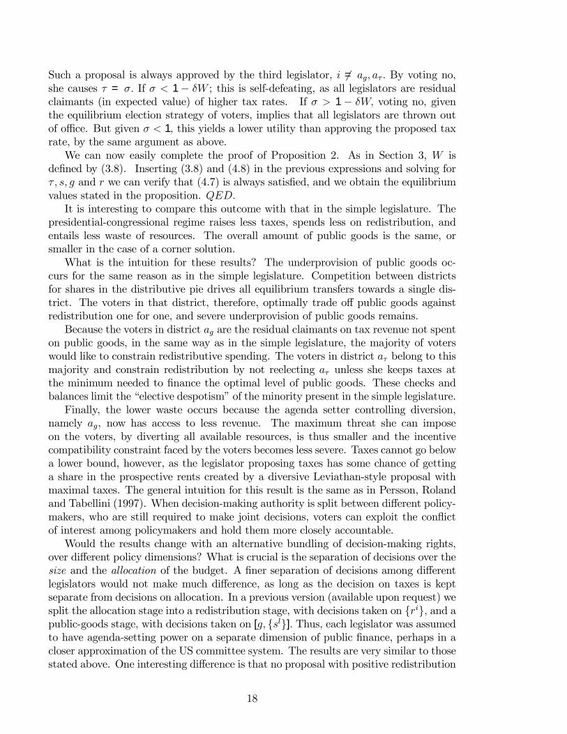
Such a proposal is always approved by the third legislator, i 6= ag, aτ . By voting no,she causes τ = σ. If σ < 1 − δW ; this is self-defeating, as all legislators are residualclaimants (in expected value) of higher tax rates. If σ > 1 − δW, voting no, giventhe equilibrium election strategy of voters, implies that all legislators are thrown outof office. But given σ < 1, this yields a lower utility than approving the proposed taxrate, by the same argument as above.We can now easily complete the proof of Proposition 2. As in Section 3, W is

defined by (3.8). Inserting (3.8) and (4.8) in the previous expressions and solving forτ , s, g and r we can verify that (4.7) is always satisfied, and we obtain the equilibriumvalues stated in the proposition. QED.It is interesting to compare this outcome with that in the simple legislature. The

presidential-congressional regime raises less taxes, spends less on redistribution, andentails less waste of resources. The overall amount of public goods is the same, orsmaller in the case of a corner solution.What is the intuition for these results? The underprovision of public goods oc-

curs for the same reason as in the simple legislature. Competition between districtsfor shares in the distributive pie drives all equilibrium transfers towards a single dis-trict. The voters in that district, therefore, optimally trade off public goods againstredistribution one for one, and severe underprovision of public goods remains.Because the voters in district ag are the residual claimants on tax revenue not spent

on public goods, in the same way as in the simple legislature, the majority of voterswould like to constrain redistributive spending. The voters in district aτ belong to thismajority and constrain redistribution by not reelecting aτ unless she keeps taxes atthe minimum needed to finance the optimal level of public goods. These checks andbalances limit the “elective despotism” of the minority present in the simple legislature.Finally, the lower waste occurs because the agenda setter controlling diversion,

namely ag, now has access to less revenue. The maximum threat she can imposeon the voters, by diverting all available resources, is thus smaller and the incentivecompatibility constraint faced by the voters becomes less severe. Taxes cannot go belowa lower bound, however, as the legislator proposing taxes has some chance of gettinga share in the prospective rents created by a diversive Leviathan-style proposal withmaximal taxes. The general intuition for this result is the same as in Persson, Rolandand Tabellini (1997). When decision-making authority is split between different policy-makers, who are still required to make joint decisions, voters can exploit the conflictof interest among policymakers and hold them more closely accountable.Would the results change with an alternative bundling of decision-making rights,

over different policy dimensions? What is crucial is the separation of decisions over thesize and the allocation of the budget. A finer separation of decisions among differentlegislators would not make much difference, as long as the decision on taxes is keptseparate from decisions on allocation. In a previous version (available upon request) wesplit the allocation stage into a redistribution stage, with decisions taken on {ri}, and apublic-goods stage, with decisions taken on [g, {sl}]. Thus, each legislator was assumedto have agenda-setting power on a separate dimension of public finance, perhaps in acloser approximation of the US committee system. The results are very similar to thosestated above. One interesting difference is that no proposal with positive redistribution

18

can get equilibrium support in Congress, so that in equilibrium, r = 0. The reasonis that the non-agenda setting legislators at the redistribution stage do not benefit(directly or indirectly) from r > 0, and would rather have the tax revenue spent on rentsfor themselves. If, however, the decision on taxes is combined with allocative decisions,we return to the equilibrium of the simple legislature. In particular, combining thedecision on (τ , g, s) and separating it from that on r would make it impossible forvoters to enforce τ < 1, as the agenda-setting legislator for τ would be the residualclaimant of higher taxes. Similarly, combining the decision on (τ , r), while keepingit separate from that on (g, s), would also break the equilibrium, since the voters ofthe legislator in charge of proposing the size of the budget would want maximal taxrevenues.The results would also change if the separation of powers was diluted by substantial

amendment rights to policy proposals, or if collusive deals could be struck betweenthe legislators. This is why sequential decision making is important; it implies thatcollusive agreements cannot be enforced. Initial promises made by ag to aτ , conditionalon the latter setting a high tax rate, are not credible, because ag has all the bargainingpower once taxes are decided. Under the reasonable assumption that contracts betweenlegislators cannot be written or enforced by third parties, enforcement of such collusivedeals would have to rely solely on reputational forces.We rule collusion out by our assumption that both legislators are included in the

winning coalition at stages (4) and (5) with equal probability. Relaxing this assumptionand allowing for a joint deviation between ag and aτ would break the equilibriumdescribed above. Indeed, if aτ is included with probability 1 in the majority coalitionby ag, then she will be fully residual claimant at the margin on any proposed increasein the tax rate.18 Therefore, voters cannot discipline her to keep the tax rate down.The fact that collusion can break the separation of powers equilibrium points to adeeper difference between the parliamentary and the presidential-congressional regimes:trying to introduce a sequential budgetary procedure in a parliamentary regime will notcreate the checks and balance effect of Proposition 2. Indeed, legislative cohesion is anendogenous outcome that sustains collusion (co-operation), due to the basic institutionsin a parliamentary regime, as we will see in the next section.Finally, we could easily allow the legislator proposing the size of the budget to be

elected on a national ballot, rather than in a district. He would then be accountableto the whole electorate, as a president or a state governor. The results would bevery similar to those of Proposition 2. The majority of voters, not benefiting fromsubsequent redistribution, would hold him accountable to propose low taxes in order todiscipline subsequent agenda setters.19 This yields a stronger and more collusion-proofseparation of powers than the one discussed in Proposition 2, since the elected presidentwill never be part of the coalition at the allocation stage. Voters can thus disciplinehim to propose a low tax rate since he is not a residual claimant on tax revenue.20 Apresident with only veto powers but no proposal rights over taxes, however, would notbe able to affect the size of government. In equilibrium he would be compensated withsome rents so as not to exercise his veto power, but without effective proposal rightshe would not be able to impose a small budget on the other legislators.

19

5. A parliamentary regime

In this section, we consider a different modification of the simple legislative game fromSection 3, which is designed to capture the essentials of a parliamentary regime. At theoutset of each period, Nature picks two legislators as members of a majority coalitionconstituting the “government”. One of these “ministers” prepares a budget proposalon behalf of the government. The proposal then goes to Parliament for a vote. In thisvote, each coalition partner has a veto right. The veto can be thought of as a vote ofconfidence on the government. If the veto is exercised, a government crisis follows. Tosimplify the analysis, we assume that in case of a government crisis, a new agenda setteris picked at random and the decision-making process reverts to the same rules as in thesimple legislature of Section 3. This may be a plausible assumption in parliamentaryregimes without a constructive vote of no-confidence.21 In any event, the assumptioncaptures the basic cost of triggering a government crisis in a parliamentary regime,namely the prospective loss of valuable proposal powers associated with ministerialportfolios. Examining public finance under alternative rules for government break-up,as in Baron (1998), is an interesting issue for further work.The specific game examined in each period is illustrated in Figure 3. It consists of

the following stages:

(0) Nature randomly selects two coalition partners (“ministers”) amongthe incumbent legislators; one becomes the agenda-setter for public financedecisions, a and the other her junior partner m.

(1) Voters set reservation utilities for their voting rule, {bi} .(2) a proposes [τ a, {ria}, ga,

nsla

o] : ra + ga + sa ≤ 3τ a.

(3) The junior coalition partner can veto the joint proposal from stage (2).If approved, the proposal is implemented and the game goes to stage (8).If not, the government falls and the game goes on to stage (4’).

(4’) Nature randomly selects a new agenda setter a0, among the three leg-islators

(5’) Voters reformulate their reelection strategies, conditional on the statusof their representative after the government crisis.

(6’) The agenda-setter a0 proposes an entire allocation qa0.

(7’) Parliament votes on this proposal. If approved by at least two leg-islators, qa0 is implemented. If not, the legislative bargaining ends and adefault outcome with τ = si = σ and g = ri = 0 is implemented.

(8) Elections are held.

Figure 3 about here

Before continuing, it is worthwhile to discuss the formulation of this game and re-late it to the previous ones. Compared to the simple legislature of Section 3, the junior

20

coalition partner has a preassigned veto right. Exercising this veto triggers a govern-ment crisis (i.e., a new game in which agenda-setting powers are reallocated) instead ofa status quo outcome. This veto right gives the junior coalition partner and the votersshe represents more bargaining power and induces legislative cohesion. Compared tothe presidential-congressional regime, voting over different policy dimensions is not se-quential. Hence there are no checks and balances and no effective separation of powers.Note that sequential proposals within government would not add any effective separa-tion of powers. As long as a veto at the last proposal stage triggers a government crisis,it would undo previous proposals since the budgetary process would have to start overagain at stage (4’). This is in accordance with the rules of a parliamentary democracy.In a previous version of the paper, we indeed considered two- and three-stage budgetpreparations within government, with separate ministers making sequential proposals.The results are identical.The previous version also expanded the legislative bargaining by adding an initial

government formation stage, where nature selects a “prime minister” who, in turn,chooses a government partner and optimally allocates the agenda-setting powers be-tween herself and the other politician. In equilibrium, the prime minister always keepsthe valuable spending portfolio to herself, since that determines who gets higher rentsin equilibrium.22

The other building blocks of the game remain the same as before. Thus, legislatorshave the same objective functions as in Section 3. Elections take place in each districtat the end of each period. Voters in each district coordinate on utility-maximizingretrospective voting strategies, conditioning their re-election on the position of theirrepresentative: outside the government, or which position if inside government (l =a,m, n), and agenda setter or not in the case a breakdown of government has occurred(l = a

0, l 6= a

0):

Dlt+1 = 1 (5.1)

if U i(qt) ≥ bi, i = l.

An equilibrium is defined as in previous sections (a precise definition can be found inthe Appendix).

The equilibrium features are summarized in the following proposition (the P su-perscript stands for parliamentary regime), which is formally proved in the Appendix:

Proposition 3. In the parliamentary regime, there is a continuum of equilibria,such that :

τP = 1 = τL > τC .

sP = 3 1−δ1−δ/3 = sL > sC , saP = 2

3sP , smP = 1

3sP

g ≥ gP > gC , with g defined by Hg(g) = 12.

rP = 2δ1−δ/3

− gP ≥ 0.

riP ≥ 0 if i = a,m, riP = 0 if i = n.

If riP > 0 for i = a,m, then gP = g

21

biP = H(gP ) + riP , ba0P = H(g0) − g0 + 2δ

1−δ/3 , b0

= H(g0) with g0 =

min{bg, 2δ1−δ/3

}All politicians are re-elected and a government crisis never occurs.

The key to understand the features of this equilibrium is the veto rights enjoyedby both coalition partners. Under the assumed timing, this veto right allows votersin the districts of a and m to demand a high share of redistribution without fearof being excluded from the coalition. In other words, bilateral monopoly replacesBertrand-competition in the determination of the redistributive budget. In equilibrium,the requests of voters in the majority districts must be mutually compatible. Thereservation utilities ba and bm can be considered as the threat points in intra-governmentbargaining, where the ministers act on behalf of their constituencies in order to earnre-election. For consistency, a higher ba is associated with a lower bm in equilibrium,and vice-versa. But this can happen in many ways. Hence the multiplicity of equilibria.These multiple equilibria thus have nothing to do with the infinite-horizon folk the-

orem (we have ruled out such multiplicity by the restriction to “historyless” strategies).Instead, they are multiple Nash equilibria in the game between voters in the differentdistricts. They are closely related to the multiple equilibria in delegation games withobservable contracts, analyzed by Fershtman, Kalai and Judd (1991). Here, the votingstrategies play the role of observable contracts.The equilibria in the parliamentary regime thus typically entail redistribution to-

wards a majority, unlike the simple legislature and the presidential-congressional regime,where any redistribution instead goes to a minority.Associated with this majority-oriented redistribution, we also find a higher provision

of public goods. Why? The equilibrium policy must be jointly optimal for the votersrepresented in the governing coalition, given that it satisfies the incentive constraintfor rents. Hence, the benefit of the public good for two out of three districts areinternalized. If the-non negativity constraints on ri do not bind, for i = a,m, publicgoods must be jointly optimal for the two groups of voters in the majority. Then, wehave: gP =g, where 2Hg(g) = 1. Public good provision falls short of this level only if thenon-negativity constraint on ri binds, either for i = ag or for i = aτ . For instance, thiscan happen if bm or ba are set exactly at E(u0). In that case, the only way of transferringutility from one group of voters to the other is to reduce spending on the public good,while at the same time increasing the transfer to the favored group. As long as theinterregional transfers after a government crisis r0 are strictly positive, however, thelevel of public goods must still be strictly higher than in the simple legislature–andthus also than in the presidential-congressional regime–because voters’ utilities mustbe at least as large as E(u0). No transfers to region m or a must then be compensatedby a higher level of public goods. Public goods at the first-best level with 3Hg = 1 cannever be an equilibrium, however.The threat of going through a government crisis, followed by a simple legislative

game with no additional constraints, enables the legislators to appropriate as muchrents as in the simple legislature, irrespective of the equilibrium tax rate. But thebargaining power of the junior partner implies that rents are more equally distributedwithin the majority. Compared to the presidential-congressional regime, the lack of

22

separation of powers implies more scope for collusion among the coalition partners.This means that politicians earn more rents in the parliamentary regime.Equilibrium taxes are also higher than in the presidential-congressional regime. Not

only do the legislators in the governing coalition have a strong selfish interest in hightaxes. But now a majority of the voters, namely the voters in districts a and m, alsobenefits from redistribution at the expense of the minority. This majority thus has astrong incentive to induce their elected representatives to maximize tax revenues.Alternative assumptions on what would happen after a government crisis would

not affect our qualitative results but would change the continuation value for individ-ual legislators and/or for voters, which would mainly affect the bargaining power ofindividual coalition partners over s.Let us close the theoretical part of the paper by a brief discussion of normative is-

sues. Since we have a characterization of the equilibria in the presidential-congressionaland in the parliamentary regime, it is tempting to ask which is better for the voters.Using the equilibrium allocation in Propositions 2 and 3 as well as in (2.2)-(2.3), we cancompute the ex ante expected utility of a voter in any of the three districts, in eachof the two regimes. Straightforward calculations give the following expected utilitydifference between the parliamentary and presidential-congressional regimes:

E(uiP )− E(uiC)] (5.2)

=1

1− δ"[(H(gP )− 1

3gP )− (H(gC)− 1

3gC)]− δ(1− δ)

(1− δ/3)(1 + 2δ/3)

#.

The first term inside the large square bracket captures the welfare effect of higher publicgoods provision and its financing under the parliamentary regime. It is always positive,as the expression H(g)− 1

3g is maximized at the socially optimal level (cf. Section 2)

and as gP > gC . The second term captures the welfare effect of the higher waste (andhigher associated taxes) under the parliamentary regime. It is always negative. Looselyspeaking, the parliamentary regime is thus better for the voters if public goods are veryvaluable (so that gP is considerably higher than gC), or if the political agency problemis small (as δ approaches unity).23

Even though we do not want to get into the difficult question about endogenousinstitutional choice in this paper, this result points towards the conditions under whichwe may observe the two regimes. Note, however, that the tension between a Pigovianand a Leviathan approach appears at the level of institutional choice as well. As rentsin our model are always higher in the parliamentary regime, that regime would alwaysbe preferred by the legislators (the expected utility difference for a legislator would justbe the negative of the second term in (5.2)). The outcome of a referendum and a votein the legislature on institutional reform might thus be very different. This, in turn,suggests that it may be unwise to delegate constitutional reforms to the same electedpolitical representatives that are supposed to choose public policy within the reformedconstitution. Constitutional reforms in the true interest of the voters are more likelyto be carried out by a Constitutional Assembly elected for that specific purpose.

23

6. Some evidence

The theory developed in the previous sections generates clear predictions on how thelevel and composition of government spending depends on the political regime. Aresuch predictions supported by empirical evidence? We report here a preliminary an-swer, drawing on a more extensive empirical analysis by Persson and Tabellini (1999b)based on data from 54 democracies.24

According to the theory, countries should be classified on the basis of two criteria:(i) whether they have institutions inducing legislative cohesion and (ii) whether thereis effective separation of powers between different political actors, with regard to de-cisions over the size and composition of spending. Our primary source for classifyingcountries along these dimensions is Shugart and Carey (1992), ch.8. With regard tolegislative cohesion, we consider rules for government formation and government ter-mination, as well as rules for the dissolution of the assembly. Countries where cabinetsurvival depends on the support of a majority in the legislature, where Parliamenthas strong rights of censure over the government, or where a directly elected Presi-dent has little influence over government formation or dismissal, are ranked as havingstronger legislative cohesion. With regard to separation of powers, we consider whetheror not there is a directly elected president and, if so, we rank his veto rights (in allpolicy dimensions) and his rights of initiative over the budget; the stronger are thesepresidential rights, the more effective is separation of powers likely to be.Combining these two dimensions, countries are classified in two groups, as parlia-

mentary or presidential-congressional regimes. The two groups have roughly the samesize (30 parliamentary and 24 presidential-congressional regimes). A detailed list isprovided in Table 1. Regimes coded as parliamentary induce legislative cohesion buthave weak separation of powers. Countries without a directly elected president endup in the parliamentary regime. The one exception is Switzerland which is includedamong the presidential-congressional regimes, as the cabinet–even though chosen bythe Assembly–has a life of its own, where survival does not depend on majority sup-port in the Assembly. Among the parliamentary regimes, however, we have includeda number of countries with a directly elected president, such as France, Finland, andPortugal. In these countries, the rules for government formation and dissolution implyconsiderable legislative cohesion. Recent periods of “cohabitation” illustrate that themajority in the French National Assembly really has more power than the elected pres-ident (see e.g. Pierce (1991)). Besides the US, many presidential regimes are found inLatin America.

Table 1 about here

Clearly, it is very difficult to pigeon-hole the observed variety of political institu-tions along a single dimension, and our classification probably entails some arbitrarydecisions. The classification is supported by the in depth investigation of Shugartand Carey (1992), however, and it is based on criteria that have no connection withthe observed fiscal policies. Of the two criteria identified by the theory, institutions

24

producing legislative cohesion and separation of budgetary powers, we are probablyweighing the former more than the latter. While the idea of legislative cohesion is inline with earlier research by political scientists, and is probably accurately captured inour classification, the notion of separation of budgetary powers has been studied byeconomists such as Von Hagen and Hallerberg (1997), but has received scant attentionby researchers in comparative politics. Further research is required to develop precisemeasures of separation of powers corresponding to the theory developed in this paper.Let us now turn to observed fiscal policy in these two country groups. Here we

mainly focus on size of government. According to the theory, legislative cohesion andlack of separation of powers in parliamentary regimes promote a larger government.For each of the 54 democracies in our sample, we measure the size of government bythe average total spending of central government, as a function of GDP, over five years,centered on 1990. Data sources and definitions are described in the Appendix.Table 1 reports the data on size of government. The difference in the size of gov-

ernment is striking. As can be seen at the bottom of Table 1, on average and withoutcontrolling for anything else, parliamentary regimes spend 17—18 percentage points ofGDP more than Congressional-Presidential regimes. Some of these differences in thesize of government may be due to other economic and social variables, unrelated tothe political regime. To control for these other determinants, we have estimated aregression of the size of government on the following variables: the log of per capitaincome (INCOME), the log of openness (OPEN), the share of the population above 65years of age (OLD), and a measure of ethno-linguistic fractionalization (ETHNO) (theAppendix gives precise definitions). As discussed in Persson and Tabellini (1999b),these variables have been included as determinants of the size of government in variousearlier cross-country studies–for instance, by Cameron (1978), Rodrik (1999), Goode(1984), Easterly and Levine (1997).The second column in Table 1 contains the estimated residuals of this regression

(omitting any measure of political regime from the specification). Some of the observeddifferences disappear, but important differences remain across regimes: the average ofthe residuals is + 2.19 among the Parliamentary regimes, it is - 2.74 among the Presi-dential systems. This difference across regimes is confirmed by a regression which, inaddition to the socio-economic control variables, also includes a dummy variable takinga value of 1 for countries classified as presidential and zero otherwise (PRES): the esti-mated coefficient on this variable is -10.0, with a t-statistic (corrected for heteroscedas-ticity) of -3.6. Thus controlling for other determinants of fiscal policy, spending bycentral government is 10 percentage points of GDP lower in presidential-congressionalregimes. Persson and Tabellini (1999b) do some sensitivity analysis, measuring spend-ing by general rather than central government, enlarging the set of economic controls,and adding dummy variables that group countries according to their geographic loca-tion or their degree of industrial development. They also control for the electoral rule.The estimated coefficient on PRES remains stable and highly significant, suggestingthat the results are very robust.The theory in this paper also has implications concerning other fiscal policy vari-

ables, in particular public good provision and wasteful government spending or out-right corruption. Both are harder to measure than the size of government. Persson

25

and Tabellini (1999b) consider a measure of public good provision, defined as the sumof spending by central government on transportation, education, and order and safety.In some specifications, public spending on health services are also included. This isclearly an imperfect measure of spending on pure public goods, since it also includeslocal public goods and redistribution in kind. Here, the evidence is much weaker.The two groups of countries spend, on average, the same amounts (as a percentage ofGDP) on these items. Controlling for other economic, social and political variables,the dummy variable PRES has a negative estimated coefficient, as expected, but it isnot statistically different from zero.Thus, the evidence suggests that the size of government is strongly affected by the

constitutional features studied in this paper, as predicted by the theory. Whether thelack of robust evidence regarding public good provision is due to poor measurement,or to a real failure of the theory, remains to be investigated more carefully. Otherpredictions of the theory, concerning wasteful spending (or, more generally, corruption)and the shape of redistributive programs, also lend themselves to empirical analysis.The encouraging results obtained for the size of government suggest that such anempirical investigation is worthwhile, and might further enhance our understanding ofthe determinants of fiscal policy choices.

7. Concluding remarks

Before sketching possible extensions of our analysis, let us consider a possible criticismof such a research program. It is related to the uneasiness sometimes expressed overgame-theoretic research in the modern literature on industrial organization. Will ourresults not be extremely sensitive to the particular extensive-form game and couldwe not “prove anything” by picking the right form? One answer is self-evident: oneshould derive and report results under different assumptions, as we have done at the endof Sections 4 and 5. Another answer is that empirical regularities found in real-worldconstitutions, rather than the researcher’s imagination, should govern the assumptions.The precise features of actual constitutions are very well documented and their essencecan often be well-captured by varying the rules of an extensive-form game. Indeed, onecan argue that comparative politics is an area where the scope for empirically guidedapplications of game theory is much greater than in industrial organization.We thus believe that the analysis in this paper can be productively extended in

different directions. One would be to introduce (in the model of Section 4) a president,and contrast a line-item veto with a veto on the entire budget. The line-item veto mightallow the president to better discipline congress, but may also make the president amore direct prey to special interests. Another direction would be to consider alterna-tive rules for government breakup observed in parliamentary regimes around the world,and ask how they would alter the trade-offs in public finance (in the model of Section5). The results in Baron (1998) suggest that different rules would fundamentally redis-tribute the bargaining powers among the members of the governing coalition. A thirdextension, motivated both by presidential regimes in Latin America and parliamentaryregimes in Europe, would be to consider electoral regimes with proportional represen-tation. In the model, proportional representation could be captured by studying one

26

district and three representatives elected in that district. This is likely to introducecompetition among voters within districts, along the lines of Ferejohn (1986) and Pers-son and Tabellini (2000). It would also be desirable (but difficult) to introduce politicalparties. These could be modeled as long-lasting coalitions of politicians that allocateagenda-setting powers taking electoral outcomes into account. With appropriate in-dividual heterogeneity within each district, these parties could then seek the supportof voters across districts. Recent work by Morelli (1998) is an example of how thesedifficult questions might be tackled in a more abstract framework.Finally, our analysis suggests difficult–but fascinating–questions regarding the

design of political institutions. These include normative questions about the optimalchoice of political system and positive questions about how to explain observed politicalreforms.

27

8. APPENDIX

8.1. Definition of equilibrium in the presidential-congressional regime

Definition 2. An equilibrium of the presidential-congressional regime is a vector ofpolicies qCt (bt) = [τCt (bt), g

Ct (τCt (bt),bt), {siCt (τCt (bt),bt)}, {riCt (τCt (bt),bt)}] and a

vector of reservation utilities bCt such that in any period t,with all players taking asgiven the expected equilibrium outcomes of periods t+ k, k ≥ 1 :

(I) for any given bt, at stage (3), at least one legislator i 6= aτ weakly prefersaccepting rather than rejecting proposal τCt , taking as given the expected equilibriumproposals and decisions at stages (4) and (5);

Definition 3. (II) for any given bt, aτ prefers proposing τCt to any other τ t satisfying(I), taking as given the expected equilibrium proposals and decisions at stages (4) and(5);

(III) for any given bt and τ t, at stage (5) at least one legislator i 6= ag weakly prefersaccepting rather than rejecting the proposalgCt (τ t(bt),bt), {siCt (τ t(bt)),bt)}, {riCt (τ t(bt)),bt)};

(IV) for any given bt and τ t, at stage (4) ag prefers the proposalgCt (τ t(bt),bt), {siCt (τ t(bt)),bt)}, {riCt (τ t(bt)),bt)} to any other proposal satisfying (III)and the budget constraint;

(V) The reservation utilities biCt are optimal for the voters, in each district i, takinginto account that policies in the current period will be set according to qCt (bt), andtaking as given the reservation utilities in other regions b−iCt as well as the identity ofaτ , ag.

8.2. Definition of equilibrium in the parliamentary regime

Definition 4. An equilibrium of the parliamentary regime is defined by qPt (bt) =[τPt (bt), {riPt (bt)}, gPt (bt), {siPt (bt)}] and the reservation utilities bPt , bP

0t , such that in

any period t, and taking as given the expected equilibrium outcomes of periods t+ k,k ≥ 1 :

(I) for any given vectors bt, and given the proposal made at stage (2), at stage (3)the junior partner of the coalition optimally chooses whether to accept or reject theseproposals, taking as given the expected reservation utilities b0t and the expected policyoutcome in stages (4’)-(7’);

(II) the reservation utilities biP0

t are optimal for the voters in each district i, after agovernment crisis at stage (3), taking into account that policies will be set accordingto q0t(b

P 0t ) as in the simple legislature equilibrium, and taking as given the reservation

utilities in other regions b−iP0

t ;((III)for any given bt and b0t, the agenda-setter in the coalition prefers qPt (bt) =[τPt (bt), {riPt (bt)}, gPt (bt), {siPt (bt)}] , given (I) and (II) and the government budgetconstraint;

(IV) The reservation utilities biPt are optimal for the voters, in each district i, takinginto account that policies in the current period will be set according to qPt (bPt ), takingas given expected bP

0t and the fact that policies will be set according to q0t(b

P 0t ) after

28

a government crisis at stage (3), and also taking as given the reservation utilities inother regions b−iPt .

8.3. Proof of Proposition 3

Equilibrium rents are given in the following:

Lemma 4. In all equilibria of the parliamentary regime, sP = 3 1−δ1−δ/3 =

sL, distributed as : saP = 23sP , smP = 1

3sP .

Proof. The equilibrium is solved by backward induction, starting from the laststages of the game and moving forward. Suppose first that a government crisis mate-rializes, so that we reach the subgame consisting of stages (4’)-(7’). By an argumentanalogous to that in Section 3, it is easily shown that g0 = Min(bg, 2δW ), τ 0 = 1,r0 = 2δW − g0, and s0 = 3 − 2δW. Note, however, that W is the equilibrium value ofholding office in the parliamentary regime, not in the simple legislature. Thus, the ex-pected continuation value of reaching this subgame (where all legislators are re-elected)for all legislators is:

E(v0) =1

3s0 + δW, (8.1)

and the expected (one-period) continuation payoff for voters in each district is:

E(u0) = H(g0) +1

3r0 = H(g0) +

1

3(2δW − g0). (8.2)

To construct the equilibrium, note first that at stage (3), m will veto any proposalthat does not give her the same value as after a government breakup. An acceptedproposal, yielding reelection, must thus satisfy sm + δW ≥ E(v0). As a will not paymore than necessary for support, this means sn = rn = 0 and by (8.1),

sm =1

3s0.

Voters will not be able to push the total equilibrium payoff for legislators below whatthey get after a government crisis, which, in turn, implies the following incentive con-straint:

s ≥ s0 = 3− 2δW (8.3)

sa = s− sm ≥ 2

3s0.

Clearly, in equilibrium the voters will not leave excess rents to the legislators, andall the weak inequalities above will hold as equalities.To conclude the argument, we solve for W from:

W (1− δ) =1

3s =

1

3s0 = 1− 2δ

3W,

29

which yields:

W =1

1− δ/3 . (8.4)

Substituting the implied value of 2δW into the expressions for s, one easily derives theequilibrium expressions for sP in Lemma 4 and Proposition 3. QED.

Inserting equilibrium rents in the government budget constraint, the remainingpolicy instruments must satisfy:

g + r = 2δW + 3(τ − 1) ≡ 2δ

1− δ/3 + 3(τ − 1), (8.5)

where the identity follows from (8.4).Here there are no other incentive constraints to worry about. The worst threat the

coalition partners could impose on voters, even if they were to collude, would be toset τ = 1, r = g = 0. But that threat is already entailed in the value for s0. Hence,a will make a proposal consistent with her constituency achieving the required level ofutility. A similar argument applies to the behavior of m at stage (3), when she decideswhether to say accept or reject the proposal of a.To characterize the equilibrium policy, we must therefore pin down the equilib-

rium reservation utilities required by the voters in the governing coalition, ba and bm.Clearly, these two reservation levels must be mutually consistent under the relevantconstraints. Specifically, in equilibrium, the reservation utility ba must be optimal forvoters in district i = a, given the equilibrium value of bm, and viceversa. But thisrequirement is satisfied by many pairs of ( ba, bm), as the voters’ reservation utilitiesare chosen simultaneously, once a government is formed. Hence, there are multipleequilibria. We can only rule out policies that, from the point of view of the votersin the governing coalition, are dominated by the outcome in the simple legislature.The reason is that a disagreement inside the coalition can bring down the government.Knowing what they can get in expected value in the event of a crisis, voters of eachmember in the governing coalition must optimally demand at least this amount fromtheir representatives. Hence, the equilibrium reservation utilities and the equilibriumpolicies must satisfy

bi ≡ 1− τ +H(g) + ri ≥ E(u0), i = a,m (8.6)

where the right hand side of (8.6) is given by (8.2).The equilibrium policy can therefore be computed as the solution of the following

optimization problem for the voters from the region of the agenda-setting minister,given any bm such that ba ≡ 1− τ +H(g) + ra ≥ E(u0) :

maxg,ra,rm,τ

[1− τ +H(g) + ra] (8.7)

s.t.1− τ +H(g) + rm ≥ bm ≥ H(g0) +1

3r0 (8.8)

τ ≤ 1 (8.9)

30

ra ≥ 0 (8.10)

rm ≥ 0. (8.11)

Replacing τ by its expression from the budget constraint τ = g3

+ ra

3+ rm

3+ 1− 2

3δW

and calling, respectively, λ, µ, νa, νm the multipliers of the constraints (8.8)—(8.11), onegets the following first order conditions:

Hg(gP )(1 + λ) =

µ

3+

1

3(1 + λ)

1− 1

3(1 + λ)− µ

3+ νa = 0

−1

3(1 + λ) + λ− µ

3+ νm = 0

yieldingλ = 1 + νa − νm (8.12)

andHg(g

P ) =1 + νa

2 + νa − νm . (8.13)

If we had τ < 1, then µ = 0,Hg(gP ) = 1

3= 1+νa

2+νa−νm from which we deduce that1 + 2νa = −νm which is impossible. Therefore, τ = 1. If νm = νa = 0, we get λ = 1and 2Hg(g

P ) = 1. If νm = 0, 12< 1+νa

2+νa < 1. If νa = 0, 12−νm > 1

2. In the latter case,

by (8.8), with r0 > 0, we must have H(g) > H(g0) where g0 = gC . Therefore, wemust have gP > gC. With r0 = 0, there is no surplus to be shared by the governmentcoalition with respect to the expected continuation payoff after a crisis E(u0) but thengP = g0 = 2δW = 2δ

1−δ/3 which is then still larger than the relevant gC = 2δ

1+2δ/3. QED.

8.4. Data sources

SIZE : total spending by central government, in percentage of GDP. Each countryobservation refers to the average of the period 1988-92. Sources. Government FinanceStatistics, IMF, and Inter-American bankINCOME: log of real per capita income in 1990. Source: Summers and Heston, PennWorld Tables, Mark 5.6 (available on line at www.nber.org)OPEN: log of (exports plus imports over GDP) in (1990). Source: see INCOME.OLD: share of population above 65 years of age, in 1985. Sources: Barro and Lee,Data Set for a Panel of 138 countries (available on line at www.nber.org), and UnitedNations Demographics Yearbook.ETHNO: Index of ethno-linguistic fractionalization in 1960. Source: Mauro (1995)

31

ReferencesAghion Philippe. and Patrick Bolton “Incomplete social contracts”. Manuscript.

London, University College London, Department of Economics, 1998.Alesina, Alberto , “Credibility and policy convergence in a two-party system with

rational voters”, American Economic Review 78 (September 1988): 796-805.Alesina, Alberto and Howard Rosenthal “A theory of divided government”, Econometrica

64 ( November 1996): 1311-1341.Banks, Jeffrey and Rangarajan Sundaram “Adverse Selection andMoral Hazard in a

Repeated Elections Model,” in Political Economy: Institutions, Information, Competition andRepresentation edited byWilliamA. Barnett, Melvin J. Hinich and Norman J. Schofield,New York, Cambridge University Press, 1993.Banks, Jeffrey and Rangarajan Sundaram “Electoral Accountability and Selection

Effects” Manuscript. University of Rochester, Department of political science, 1996.Baron, David “Comparative dynamics of parliamentary government”, American Political Science

Review 92 (September 1998): 593-610.Baron, David and John Ferejohn , “Bargaining in legislatures”, American Political Science

Review 83 (December 1989): 1181-1206.Barro, Robert , “The control of politicians: an economic model”, Public Choice 14

(Spring 1973): 19-42.Besley, Timothy and Stephen Coate , “An economic model of representative democ-

racy”, Quarterly Journal of Economics 112 ( February 1997): 85-114.Brennan, Geoffrey and James M. Buchanan The Power to Tax, Cambridge: Cam-

bridge University Press, 1980.Cameron, David , “The expansion of the public economy: A comparative analysis”,

American Political Science Review 72 (December 1978): 1203—1261.Chari, V.V, Larry E. Jones, and Ramon Marimon , “The economics of split voting

in representative democracies”, American Economic Review 87 (December 1997): 957-76.Diermeier, Daniel and Timothy J. Feddersen , “Cohesion in legislatures and the vote

of confidence procedure”, American Political Science Review 92 ( September 1998):611-621.Dixit, Avinash The Making of Economic Policy: A Transaction-Cost Politics Perspective,

Cambridge: MIT Press, 1996.Dixit, Avinash and John Londregan , “The determinants of success of special inter-

est groups in redistributive politics ” Journal of Politics 58 (November 1996): 1132-55.Downs, Anthony An Economic Theory of Democracy New York: Harper and Row,

1957.Easterly, William and Ross Levine , “Africa’s growth tragedy: Policies and ethnic

divisions”, Quarterly Journal of Economics 112( November 1997): 1203-50.Ferejohn, John , “Incumbent performance and electoral control”, Public Choice 50

(Spring 1986): 5-26.Fershtmann, Chaim, Kenneth L. Judd and Ehud Kalai , “Observable contracts:

Strategic delegation and cooperation”, International Economic Review 32 (August 1991):551-559.

32

Goode, Richard , Government Finance in Developing Countries , Brookings Insti-tution: Washington D.C. 1984.Grossman, Gene and Elhanan Helpman , “Protection for sale”, American Economic Review

84 ( September 1994): 833-50.Grossman, Gene and Elhanan Helpman , “Electoral competition and special interest

politics, Review of Economic Studies 63 (April 1996): 265-86.Hallerberg, Mark and Jürgen von Hagen, “Electoral Institutions, Cabinet Negotia-

tions, and Budget Deficits within the European Union ” CEPR Discussion Paper No1555, 1997.Hart, Oliver , Firms, Contracts and Financial Structure, Oxford: Oxford Univer-

sity Press, 1995.Huber, John , “The vote of confidence in parliamentary democracies ”, American Political Science

Review 90 (June 1996), 269-282.Laver, Michael and Kenneth Shepsle Making and Breaking Governments: Cabinets

and Legislatures in Parliamentary Democracies, New York: Cambridge UniversityPress, 1996.Levitt, Stephen and James Snyder , “The impact of federal spending on house

election outcomes“, Journal of Political Economy 105 (February 1997), 30-53.Lewis-Beck, M. , Economics and Elections: The Major Western Democracies, Ann

Arbor: University of Michigan Press, 1988.Lijphart, Arend. (ed.) Parliamentary versus Presidential Government, Oxford:

Oxford University Press, 1992.Lindbeck, A, and J. Weibull , “Balanced budget redistribution as the outcome of

political competition”, Public Choice 54 (Spring 1987), 273-97.Mauro, Paolo “Corruption and growth”, Quarterly Journal of Economics 105 (Au-

gust 1995), 681—712.Mauro, Paolo , “Corruption and the composition of government expenditure”,

Journal of Public Economics 69 (August 1998), 263—80.Meltzer, Allan H. and Scott F.. Richard , “A rational theory of the size of govern-

ment”, Journal of Political Economy 89 ( October 1981), 914-27.Morelli, Massimo , “Equilibrium party structure and policy outcomes under differ-

ent electoral systems”, Manuscript, Iowa State University, Department of Economics,1998.Mueller, Dennis (ed.) Perspectives on Public Choice, (Cambridge University Press:

Cambridge) (1997).Persson, Torsten , “Economic policy and special interest politics”, Frank Paish

Lecture, Economic Journal 108 (1998), 310-27.Persson, Torsten, Gerard Roland, and Guido Tabellini , “Separation of powers and

political accountability”, Quarterly Journal of Economics 112 (November 1997), 1163-1203.Persson, Torsten and Guido Tabellini “Political Economics and Public Finance”,

in: A. Auerbach and M. Feldstein eds., Handbook of Public Economics, Vol IIII, NorthHolland, forthcoming 1999a.Persson, Torsten and Guido Tabellini “The size and scope of government: Compara-

tive politics with rational politicians”, 1998Marshall Lecture, European Economic Review,

33

(April 1999b): 699-736.Persson, Torsten and Guido Tabellini Political Economics - Explaining Economic

Policy, (MIT Press, Boston), forthcoming 2000Pierce, Roy , “The executive divided against itself: Cohabitation in France, 1986-

1988”, Governance: An International Journal of Policy and Administration 4 (July 1991):270-294.Polo, Michele , “Voters’heterogeneity, electoral competition and political rents”,

Manuscript. Milan IGIER, Department of Economics, 1998.Rodrik, Dani , “Why do more open economies have bigger governments?” Journal of Political

Economy 106 (October 1998), 997—1032.Shugart, Matthew and John Carey Presidents and Assemblies: Constitution Design and Electoral

Dynamics, Cambridge: Cambridge University Press,1992.Svensson, Jakob , “The control of public policy: Electoral competition, polarization

and primary elections, Manuscript. World Bank, 1997.Tanzi, Vito and Hamid Davoodi , “Corruption, public investment and growth”,

IMF Working paper 97/139, 1997.Tanzi, Vito and Ludger Schuknecht , “The growth of government and the reform

of the state in industrial countries”, Manuscript. IMF, 1995.Tanzi, Vito and Ludger Schuknecht, “Reconsidering the fiscal role of government:

The international perspective”, American Economic Review 87( March 1997): 164-168.

34

Notes

1We are grateful for helpful comments by two anonymous referees, Micael Cas-tanheira, Elhanan Helpman, Massimo Morelli, Michele Polo, Antonio Rangel, HowardRosenthal, John Spicer and the participants in seminars at Harvard, Princeton, NYU,Stockholm, Helsinki, Uppsala, Brussels, Toulouse, Northwestern, Minnesota, the Bankof England, Tilburg, Southampton, Leuven, Mannheim, Berkeley, San Diego, USC,Michigan and in the ESF conference on Political economy, Florence, June 4-8 1997.This research is supported by grants from the European Commission (TMR FMRXCT96-0028), the Bank of Sweden Tercentenary Foundation, Bocconi University, andthe Belgian Office of Scentific, Technical and Cultural Affairs (PAI P4/28). Editor-ial assistance was provided by Christina Lönnblad and research assistance by MarcusSalomonsson.

2The data are taken from Tanzi and Schuknecht (1995, 1997).3See Dixit (1996), Persson and Tabellini (1999a), Persson and Tabellini (2000) and

the contributions in Mueller (1997) for recent surveys of positive modeling of publicfinance in political economics and public choice.

4This is in close parallel to incomplete contract theory as applied to the governanceof firms (see Hart (1995)), which deals with the consequences for firm decisions ofthe precise allocation of decision-making authority to different stakeholders, such asowners, managers, and creditors.

5Naturally, not all parliamentary regimes exhibit the same degree of legislativecohesion, because rules for government breakup and formation differ across countries(see Huber (1996) and Baron (1998)). Similarly, not all presidential regimes entailthe same separation of powers: in the French fifth republic, agenda setting powersrest within the government, which, in turn, is accountable to the legislature; in manyLatin-American countries, the legislatures have much weaker powers relative to thepresident than in the US. See also Lijphart (1992) and Shugart and Carey (1992) forfurther discussion of these issues.

6Compared to Diermeier and Feddersen (1998), our model is deterministic andcontinuation values after a government crisis are obtained via a simpler continuationgame.

7Tanzi and Davoodi (1997) and Mauro (1998) provide empirical evidence consistentwith this hypothesis: within OECD countries, as well as in a larger sample, variousforms of corruption are indeed strongly associated with expenditure on public projectsand infrastructures or with purchases of intermediate goods.

8Formally, we can think of the rents slt as adding to the legislators’ consumption.The linear expression in (3.2) is then consistent with legislators having linear utility ofconsumption, as have the voters. The legislators’ utility function would coincide withthe utility function of voters in (2.2), if we added the concave utility of public goods; weomit this term, however, to simplify the analysis. As discussed in Persson and Tabellini(1999a), it would be straightforward to add exogenous benefits from holding office asan additional motive for re-election and transaction costs in the diversion technology,so that politicians only capture a fraction of the resources diverted from voters.

9This framework, adapted from Ferejohn (1986), may appear special to some read-

35

ers. We believe that many of our general results on comparative politics are likelyto survive under a variety of assumptions about the motivation of politicians. Asdemonstrated in Persson (1998) and Persson and Tabellini (1999a), similar results em-anate from a legislative bargaining framework, whether interest groups lobby finance-motivated legislators, or prospectively elect outcome-motivated legislators, rather thanretrospectively reelect office-motivated legislators, as in this model.

10All qualitative results are valid if one assumes that the default diversion value σis equal to zero. In the analysis, we keep σ > 0, since it allows us to better understandthe effect of the default diversion.

11Persson and Tabellini (1999a), (1999b), following Polo (1998) and Svensson (1997),discuss a setting with probabilistic voting, where endogenous rents from office are notdissipated by electoral competition, even if candidates can make binding commitmentsbefore the elections. This happens because alternative political candidates are not per-fect substitutes for each other, so that the probability of winning the election does notdiscontinuously jump to zero for the candidate announcing marginally higher rents forherself.

12Retrospective voting conditional on economic outcomes has empirical support; seeLewis-Beck (1988) for general evidence. More specifically, Levitt and Snyder (1997)demonstrate how US federal dollars spent in a house district has a strong impact onthe vote share of the incumbent (they also show, however, that direct transfers–thespecific policy instrument of redistributive spending in our model–does not affect thisvote share).

13Banks and Sundaram (1993, 1996) formulate retrospective voting models withheterogeneity among candidate types together with asymmetric information over types.

14To simplify the analysis, we assume that the parameters are such that in equilib-rium σ ≥ δW, to ensure that the non-negativity constraint on sm is satisfied - other-wise, the qualitative results would hold, but the algebra would differ slightly. Giventhe equilibrium expression of W derived below, this assumption can also be stated as:σ ≥ δ

1−δ/3 .15As remarked above, the voting rule is ex-post (weakly) optimal, since the in-

cumbent and the opponent are identical in each district. Hence, even without theassumption that voters are committed to their voting rule, the equilibrium would stillbe sequentially rational (though many other equilibria would also exist).

16Persson and Tabellini (2000, chap 10) study a simplified version of this modelwhere rents in the default policy at stage (5) do not depend on the tax rate from stage(3). In this case there are multiple equilibria, but each of these share the qualitativeproperties with the unique equilibrium of the present model.

17Faced with a tax rate τ d > τC , the next agenda setter ag could seek reappointmentby setting ra = rC+ τd− τC , thereby neutralizing the effects of the previous deviationon her voters. But it is easy to see that ag would always prefer to exploit the hightaxes to her advantage and forgo reappointment. The intuitive reason is that inequilibrium, ag must be indifferent between seeking reappointment or not. Hence, ahigher tax rate provides more opportunities for diversion and tilts the balance in favorof no reappointment.

18If γ is the probability that aτ is included in the coalition by ag at the allocation

36

stage, then (4.8) would become τC = 1− 1−γγδW < 1 as long as γ < 1 but τC = 1 for

γ = 1.19Persson, Roland and Tabellini (1997) discuss the checks and balances associated

with sequential budgeting in a presidential system. Chari, Jones and Marimon (1997)obtain a related result in a setting with prospective voters and outcome-oriented politi-cians: by endogenously electing a “fiscally conservative” president, voters collectivelymanage to control the overspending of a Congress, to which every district finds itindividually optimal to elect a “maximally spendthrift” representative.

20The incentive constraint is then such that the two legislators other than ag mustbe convinced to vote in favor of τC , proposed by the president. It can be shown thatwhen each of these has an equal probability of being included in the coalition at theallocation stage, (4.8) becomes τC = σ − δW, which for σ < 1 is smaller than in (4.8).

21Huber (1996) uses the same short-cut to approximate the consequences of a voteof confidence procedure on government decisions in a parliamentary system.

22Laver and Shepsle (1996) provide an exhaustive treatment of a considerably richerformal model of government formation. But in their formal analysis, they ignore boththe electoral stage and the treatment of government proposals in parliament.

23Aghion and Bolton (1998) provide another example of a normative comparisonbetween alternative political constitutions. They compare alternative required majori-ties to change the status quo, and show that contractual incompleteness can give riseto an ex-ante preference for a majority rule, and more generally for decision-makingrules weaker than unanimity. Even though they focus on contractual incompleteness,they consider a model of direct democracy where agency problems between voters andpoliticians do not arise.

24We classify a country as a democracy if it scores between 1 and 5 according to theGastil (1987) index of political rights, on average over the period 1985-90. This selectioncriterion picks out 64 countries; for 10 of these, however, data on fiscal outcomes ornecessary control variables are not available.

37

a { bi } [τ, g,{ ri} , {sl} ]

(Y,Y,• ) (N,N,• )

Implement τ = sl = σ > 0

g = ri = 0

Nature Voters Legislaturevotes

Electionsa

Figure 1

(aτ , ag) { bi} [g, { ri} , { sl} ]

(N,N,• )

Implement g = ri = 0

sl = τ > 0

Nature Voters Congressvotes

Electionsaτ

τ

(Y,Y,• )

Implement τ = σ < 1

agCongressvotes

(Y,Y,• ) (N,N,• )

Figure 2

(a , m) { bi}

No

Implement

Nature Voters m Electionsa

[τ, g, { ri} , {sl} ]

Yes

Government crisis

• Nature: a’• Voters: { b’ i }• a’ : q’• Parliament votes

(Y,Y• )

Implement

(N,N,• )

τ = sl = σg= ri = 0

Figure 3

Figure 4Size of Government

-20

0

20

40

% of GDP

Parliamentary regimes Presidential regimes

Total expendituresParliamentary residualsPresidential residuals

Table 1Parliamentary Regime Presidential Regime

Country Size Residual Country Size ResidualU.K. 37.81 -1.09 U.S.A. 24.04 -1.94AUSTRIA 39.23 -2.99 SWITZERLAND 24.20 -15.58BELGIUM 50.03 5.94 ARGENTINA 10.12 -9.09DENMARK 40.49 -1.59 BOLIVIA 13.67 -4.13FRANCE 43.26 8.36 BRAZIL 30.47 17.91WEST GERMANY 30.47 -10.66 CHILE 20.67 -6.99ITALY 48.43 13.26 COLOMBIA 13.99 -6.20LUXEMBOURG 46.89 -0.52 COSTA RICA 24.98 -1.27NETHERLAND 52.95 11.80 DOMINICAN R. 14.77 -8.71NORWAY 44.16 -0.63 ECUADOR 14.19 -7.26SWEDEN 43.17 -2.49 EL SALVADOR 11.19 -9.16CANADA 23.14 -6.06 GUATEMALA 10.63 -6.40JAPAN 16.12 -10.01 MEXICO 21.07 3.31FINLAND 34.17 -1.03 NICARAGUA 31.03 8.32GREECE 51.54 13.74 PARAGUAY 10.96 -14.27ICELAND 33.14 -1.85 PERU 12.43 -2.10IRELAND 41.68 1.70 URUGUAY 26.95 -5.39MALTA 41.26 0.11 VENEZUELA 23.01 -0.38PORTUGAL 43.37 4.42 EGYPT 33.35 8.19SPAIN 33.89 2.77 SRI LANKA 29.30 5.09AUSTRALIA 26.59 -1.48 KOREA REP. 16.03 -9.72NEW ZEALAND 41.62 9.53 NEPAL 17.56 3.35BARBADOS 33.41 -3.64 PHILIPPINES 18.50 -1.42TRINIDAD & TO 33.47 7.75 GAMBIA 23.48 -1.93CYPRUS (G) 29.82 -7.81ISRAEL 47.98 15.71INDIA 17.41 6.58MALAYSIA 28.18 0.24BOTSWANA 32.60 5.97PAPUA N. GUIN 32.56 9.72AVERAGE 37.29 2.19 AVERAGE 19.86 -2.74

Data on government size refer to total expenditures by central government on averagebetween 1988-92.

Residuals for government size have been generated by the following (OLS) regressionestimated on the full sample:SIZE = -14.08(-0.73) + 0.02(0.01) * INCOME + 8.01(4.23) * OPEN + 152.9(3.51) * OLD - 0.06(-1.24) * ETHNO(t-statistics in brackets).Adjusted R2=0.57

Data sources in the Appendix.