Penalized Maximum Likelihood Estimation of Two … Reports/Technical Reports 2007-/TR... ·...

Penalized Maximum Likelihood Estimation ofTwo-Parameter Exponential Distributions

A PROJECT

SUBMITTED TO THE FACULTY OF THE GRADUATE SCHOOL

OF THE UNIVERSITY OF MINNESOTA

BY

Mengjie Zheng

IN PARTIAL FULFILLMENT OF THE REQUIREMENTS

FOR THE DEGREE OF

MASTER OF SCIENCE

Advisor: Yongcheng Qi

May, 2013

c© Mengjie Zheng 2013

ALL RIGHTS RESERVED

Acknowledgements

I would like to express my sincere appreciation to my advisor, Professor Yongcheng Qi,

for his guidance, support, encouragement, and great patience to me all the way through

my graduation process.

I am very grateful to the members of my supervisory committee: Professor Kang L.

James and Professor Richard Green for serving on my examination committee.

I would like to thank Professor Kang James for giving me precious practice and

advice, and help me out all along the seminar.

i

Abstract

The two-parameter exponential distribution has many applications in real life. In this

project we consider estimation problem of the two unknown parameters. The most

widely used method Maximum Likelihood Estimation(MLE) always uses the minimum

of the sample to estimate the location parameter, which is too conservative. Our idea

is to add a penalty multiplier to the regular likelihood function so that the estimate of

the location parameter is not too close to the sample minimum. The new estimates for

both parameters are unbiased and also Uniformly Minimum Variance Unbiased Estima-

tors(UMVUE). The penalized MLE for incomplete data is also discussed.

ii

Contents

Acknowledgements i

Abstract ii

List of Tables iv

1 Introduction 1

2 Estimation for Complete Data 3

2.1 MLE for complete data . . . . . . . . . . . . . . . . . . . . . . . . . . . 3

2.2 Penalized MLE for complete data . . . . . . . . . . . . . . . . . . . . . . 6

3 Estimation for Incomplete Data 10

3.1 MLE for incomplete data . . . . . . . . . . . . . . . . . . . . . . . . . . 11

3.2 Penalized MLE for Incomplete Data . . . . . . . . . . . . . . . . . . . . 13

4 Simulation Results 17

4.1 Simulation for complete data . . . . . . . . . . . . . . . . . . . . . . . . 17

4.2 Simulation for incomplete data . . . . . . . . . . . . . . . . . . . . . . . 19

References 22

Appendix A. R code 23

iii

List of Tables

4.1 The biases and MSEs of estimators for complete data . . . . . . . . . . 18

4.2 The biases and MSEs of estimators for Type-II HCS, with n = 10 . . . . 19



iv

Chapter 1

Introduction

Consider a random variableX having two-parameter exponential distribution EXP(θ, η),

with probability density function(pdf) given by

f (x; θ, η) =

1

θe−(x−η)/θ x > η,

0 otherwise,

(1.1)

where θ > 0 is a scale parameter and η ∈ R is a location parameter. The cumulative

distribution function (CDF) is

F (x) = P [X 6 x] =

∫ x

η

1

θe−(x−η)/θdx = 1− e−(x−η)/θ, x > η. (1.2)

The two-parameter exponential distribution has many real world applications. It

can be used to model the data such as the service times of agents in a system (Queuing

Theory), the time it takes before your next telephone call, the time until a radioactive

particle decays, the distance between mutations on a DNA strand, and the extreme

values of annual snowfall or rainfall.

Given a sample of size n from a two-parameter exponential distribution, we are

interested in estimating both θ and η. The most widely used method to do estimation

is Maximum Likelihood Estimation(MLE). Under some regularity conditions, the MLE

method has nice properties such as consistency and efficiency. The regular MLE is

too conservative because it always chooses the minimum of the sample to estimate the

location parameter. Our idea is to add a penalty multiplier to the regular MLE. By

1

2

introducing a proper penalty, the penalized maximum likelihood estimators for both

parameters are Uniformly Minimum Variance Unbiased Estimators (UMVUE).

The rest of the project is organized as follows. In chapter 2, for complete data set,

we first introduce the conventional MLE and penalized MLE. In chapter 3, we consider

incomplete data including Type-II censoring and Type-II hybrid censoring, and extend

the penalized MLE to do estimation for incomplete data. In chapter 4, we present the

simulation results for regular and penalized MLE for both complete and incomplete

data sets, and give analysis of these results.

Chapter 2

Estimation for Complete Data

In this chapter, we introduce the likelihood function and penalized likelihood function.

Then we discuss the properties of both regular and penalized likelihood estimators from

the two-parameter exponential distributions.

2.1 MLE for complete data

Maximum likelihood estimation (MLE) is a method to provide estimates for the

parameters of a statistical model by maximizing likelihood functions. For an indepen-

dent and identically distributed(i.i.d) sample x1, x2, · · · , xn with pdf as (1.1), the joint

density function is

f (x1, x2, · · · , xn | θ, η) = f (x1 | θ, η) f (x2 | θ, η) · · · f (xn | θ, η) .

A likelihood function provides a look at the joint density function from a different

perspective by considering the observed values x1, x2, · · · , xn to be fixed, while θ and η

are the variables of the function. The likelihood function is

L (θ, η | x1, x2, · · · , xn) =n∏i=1

f (xi | θ, η) =1

θne−

1

θ

n∑i=1

(xi−η), x1:n > η,

where x1:n 6 x2:n 6 · · · 6 xn:n are order statistics based on x1, x2, · · · , xn, and x1:n is

the minimum of the sample. Note that x1:n > η is equivalent to xi > η for all i.

3

4

It is more convenient to work with the logarithm of the likelihood function.

lnL (θ, η | x1, x2, · · · , xn) =n∏i=1

ln f (xi | θ, η)

= −1

θ

n∑i=1

xi +nη

θ− n ln θ, x1:n > η.

(2.1)

The likelihood function is maximized with respect to η by taking η = x1:n. To maximize

relative to θ, differentiate (2.1) with respect to θ and solve the equation

d lnL (θ, η)

dθ= −n

θ+

n∑i=1

(xi − η)

θ2= 0.

The MLE for θ is given by

θ =

n∑i=1

(xi − η)

n= x− η = x− x1:n. (2.2)

The CDF of x1:n is

F(1)(x) = P (x1:n 6 x) = 1− P (x1:n > x)

= 1− P (all xi > x) = 1− (1− F (x))n

= 1− e−n(x−η)/θ,

with the pdf given by

f(1)(x) = F ′(1)(x) =n

θe−n(x−η)/θ. (2.3)

From (2.3), x1:n ∼ EXP

(θ

n, η

).

An estimator θ is said to be an unbiased estimator of θ if E(θ) = θ for all θ.

Otherwise, θ is said to be a biased estimator of θ, and the bias is b(θ) = E(θ) − θ.The mean square error(MSE) of θ is MSE(θ) = E[θ − θ]2 = Var(θ) + [b(θ)]2.

The expectations of η and θ are

E (η) = E (x1:n) =θ

n+ η 6= η, (2.4)

and

E(θ) = E (x− x1:n) = θ + η −(θ

n+ η

)= θ − θ

n6= θ. (2.5)

5

By (2.4) and (2.5), η and θ are not unbiased estimators. And the biases are

b (η) = E (η)− η =θ

n+ η − η =

θ

n, (2.6)

and

b(θ) = E(θ)− θ = θ − θ

n− θ = − θ

n. (2.7)

Note that the traditional MLE of η picks the smallest value of the sample to estimate

the location parameter. It always overestimates the location parameter since P (x1:n >

η) = 1.

The variance of η is

Var (η) = Var (x1:n) =θ2

n2, (2.8)

which follows from the fact that x1:n ∼ EXP

(θ

n, η

).

The variance of θ is

Var(θ) = Var(x− x1:n) =n− 1

n2θ2. (2.9)

This result is obtained as follows:

Var(θ) = Var (x− x1:n) = Var (x) + Var (x1:n)− 2Cov (x, x1:n) ,

Cov (x, x1:n) = Cov

(n∑i=1

xi/n, x1:n

)=

1

n

n∑i=1

Cov (xi, x1:n)

=1

n

(n

1

)Cov (x1:n, x1:n) = Var (x1:n) ,

(2.10)

Var(θ) = Var (x) + Var (x1:n)− 2Var (x1:n) =θ2

n− θ2

n2=n− 1

n2θ2.

From (2.6), (2.7), (2.8), (2.9), the MSEs of η and θ are

MSE (η) = Var (η) + [b (η)]2 =θ2

n2+

(θ

n

)2

= 2θ2

n2, (2.11)

and

MSE(θ) = Var(θ) + [b(θ)]2 =n− 1

n2θ2 +

(− θn

)2

=θ2

n. (2.12)

6

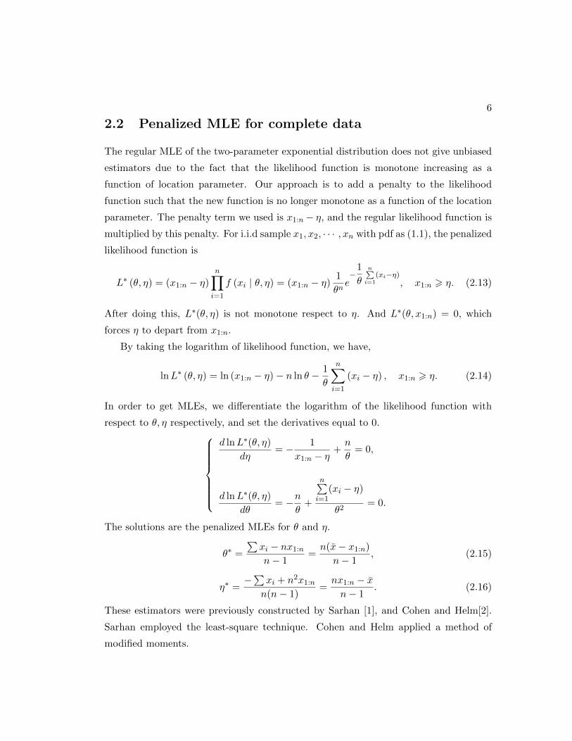
2.2 Penalized MLE for complete data

The regular MLE of the two-parameter exponential distribution does not give unbiased

estimators due to the fact that the likelihood function is monotone increasing as a

function of location parameter. Our approach is to add a penalty to the likelihood

function such that the new function is no longer monotone as a function of the location

parameter. The penalty term we used is x1:n − η, and the regular likelihood function is

multiplied by this penalty. For i.i.d sample x1, x2, · · · , xn with pdf as (1.1), the penalized

likelihood function is

L∗ (θ, η) = (x1:n − η)

n∏i=1

f (xi | θ, η) = (x1:n − η)1

θne−

1

θ

n∑i=1

(xi−η), x1:n > η. (2.13)

After doing this, L∗(θ, η) is not monotone respect to η. And L∗(θ, x1:n) = 0, which

forces η to depart from x1:n.

By taking the logarithm of likelihood function, we have,

lnL∗ (θ, η) = ln (x1:n − η)− n ln θ − 1

θ

n∑i=1

(xi − η) , x1:n > η. (2.14)

In order to get MLEs, we differentiate the logarithm of the likelihood function with

respect to θ, η respectively, and set the derivatives equal to 0.

d lnL∗(θ, η)

dη= − 1

x1:n − η+n

θ= 0,

d lnL∗(θ, η)

dθ= −n

θ+

n∑i=1

(xi − η)

θ2= 0.

The solutions are the penalized MLEs for θ and η.

θ∗ =

∑xi − nx1:nn− 1

=n(x− x1:n)

n− 1, (2.15)

η∗ =−∑xi + n2x1:nn(n− 1)

=nx1:n − xn− 1

. (2.16)

These estimators were previously constructed by Sarhan [1], and Cohen and Helm[2].

Sarhan employed the least-square technique. Cohen and Helm applied a method of

modified moments.

7

Theorem 1. (Sarhan[1]) θ∗ and η∗ are unbiased and uniformly minimum variance

estimators for θ and η.

The expectations for the penalized MLEs are

E(θ∗) = E

[n(x− x1:n)

n− 1

]=

n

n− 1

(θ + η −

(θ

n+ η

))= θ, (2.17)

and

E (η∗) = E

[nx1:n − xn− 1

]=

1

n− 1(nE(x1:n)− x)

=1

n− 1

(n

(θ

n+ η

)− (θ + η)

)=

1

n− 1(nη − η) = η.

(2.18)

From (2.17), (2.18), θ∗ and η∗ are unbiased estimators for θ and η. And thus the

biases are

b (θ∗) = E (θ∗)− η = 0, (2.19)

and

b (η∗) = E (η∗)− η = 0. (2.20)

The variance of θ∗ is

Var (θ∗) = Var

(n (x− x1:n)

n− 1

)=

n2

(n− 1)2(Var (x) + Var (x1:n)− 2Cov (x, x1:n))

=n2

(n− 1)2(Var (x) + Var (x1:n)− 2Var (x1:n))

=n2

(n− 1)2

(θ2

n+θ2

n2− 2

θ2

n2

)=

θ2

n− 1.

(2.21)

The variance of η∗ is

Var (η∗) = Var

(nx1:n − xn− 1

)=

1

(n− 1)2Var(nx1:n − x)

=1

(n− 1)2(n2Var (x1:n) + Var (x)− 2Cov (nx1:n, x)

)=

1

(n− 1)2(n2Var (x1:n) + Var (x)− 2nVar (x1:n)

)=

1

(n− 1)2

(n2θ2

n2+θ2

n− 2n

θ2

n2

)=

θ2

n (n− 1).

(2.22)

8

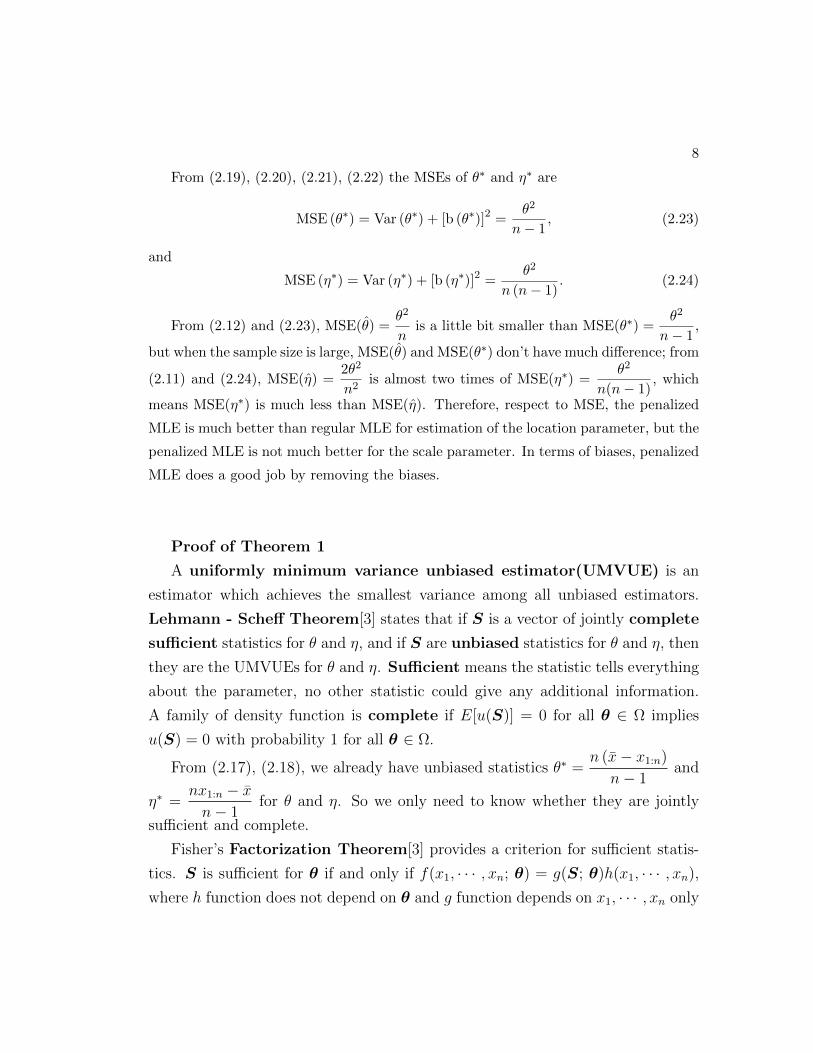
From (2.19), (2.20), (2.21), (2.22) the MSEs of θ∗ and η∗ are

MSE (θ∗) = Var (θ∗) + [b (θ∗)]2 =θ2

n− 1, (2.23)

and

MSE (η∗) = Var (η∗) + [b (η∗)]2 =θ2

n (n− 1). (2.24)

From (2.12) and (2.23), MSE(θ) =θ2

nis a little bit smaller than MSE(θ∗) =

θ2

n− 1,

but when the sample size is large, MSE(θ) and MSE(θ∗) don’t have much difference; from

(2.11) and (2.24), MSE(η) =2θ2

n2is almost two times of MSE(η∗) =

θ2

n(n− 1), which

means MSE(η∗) is much less than MSE(η). Therefore, respect to MSE, the penalized

MLE is much better than regular MLE for estimation of the location parameter, but the

penalized MLE is not much better for the scale parameter. In terms of biases, penalized

MLE does a good job by removing the biases.

Proof of Theorem 1

A uniformly minimum variance unbiased estimator(UMVUE) is an

estimator which achieves the smallest variance among all unbiased estimators.

Lehmann - Scheff Theorem[3] states that if S is a vector of jointly complete

sufficient statistics for θ and η, and if S are unbiased statistics for θ and η, then

they are the UMVUEs for θ and η. Sufficient means the statistic tells everything

about the parameter, no other statistic could give any additional information.

A family of density function is complete if E[u(S)] = 0 for all θ ∈ Ω implies

u(S) = 0 with probability 1 for all θ ∈ Ω.

From (2.17), (2.18), we already have unbiased statistics θ∗ =n (x− x1:n)

n− 1and

η∗ =nx1:n − xn− 1

for θ and η. So we only need to know whether they are jointly

sufficient and complete.

Fisher’s Factorization Theorem[3] provides a criterion for sufficient statis-

tics. S is sufficient for θ if and only if f(x1, · · · , xn; θ) = g(S; θ)h(x1, · · · , xn),

where h function does not depend on θ and g function depends on x1, · · · , xn only

9

through S.

f (x1, x2, · · · , xn | θ, η) =1

θne−

1

θ

(n∑

i=1xi−nη

)x1:n > η

=1

θnexp

[nηθ

]exp

[−

n∑i=1

xi/θ

]I(η,∞) (x1:n)

(2.25)

This satisfies the Factorization Criterion equation with h(x1, · · · , xn) = 1 and

g(s; θ, η) depends on x1, · · · , xn only through x1:n andn∑i=1

xi. So x1:n andn∑i=1

xi

are joint sufficient statistics for θ and η. Notice that θ∗ and η∗ correspond to a

one-to-one transformation of x1:n andn∑i=1

xi, so θ∗ and η∗ are jointly sufficient for

θ and η.

It follows from [4] that x1:n andn∑i=1

(xi−x1:n) jointly complete of θ and η. Note

that θ∗ and η∗ are one-to-one function of x1:n andn∑i=1

(xi− x1:n). So θ∗ and η∗ are

jointly complete for θ and η. Thus we conclude that θ∗ and η∗ are UMVUE for θ

and η.

Chapter 3

Estimation for Incomplete Data

In real life, sometimes it is hard to get a complete data set; often the data are

censored. Scientific experiments might have to stop before all items fail because

of the limit of time or out of money. Type-I and Type-II censoring are the most

basic among the different censoring schemes. Type-I censoring happens when

the experimental time T is fixed, but the number of failures is random. Type-II

censoring occurs when the number of failures r is fixed, the experimental time

is random.

Hybrid censoring is a mixture of Type-I and Type-II censoring scheme. Type-

I hybrid censoring(Type-I HCS)[5] considers the experiment being terminated

at a random time point T ∗ = minTr:n, T, where T ∈ (0,∞) is a pre-determined

time and r is a predetermined number of failures out of total n items, where

1 ≤ r ≤ n. Under this method, the experiment time will be no more than T ,

which leads to a problem that there might be very few failures that occur before

time T , which may result in extremely low efficiency of estimation. Because of

that, in this paper, we choose Type-II hybrid censoring (Type-II HCS)[6],

the experiment ends at a random time T ∗ = maxTr:n, T, where again T and r

are predetermined. This scheme guarantees that at least r failures are observed.

And it may be applied in the situation that at least r failures must be observed.

If r failures happen before time T , the experiment can continue up to time T to

make full use of the facility; if the rth failure does not occur before time T , then

10

11

the experiment has to continue until the rth failure.

In this chapter, the maximum likelihood method and penalized method are

investigated for data from two-parameter exponential distributions under Type-II

hybrid censoring. A special case of Type-II hybrid censoring is also discussed.

3.1 MLE for incomplete data

Let T be a pre-chosen experimental time, r be a pre-determined number of items

out of total n items. If, at the end of experiment, there is only one observation,

then it will be impossible to do estimation since we need to estimate two pa-

rameters. Therefore, it is reasonable to assume that at least two failures must

be observed, that is, r > 2. The experiment ends at time T ∗ = maxxr:n, T.Let N be the number of failures that happen before time T , that is, N =∑n

i=1 Ixi < T. Let r∗ be the number of observations when the experiment

stopped, r∗ = maxr,N. The Type-II hybrid censoring likelihood function of

the observed data is given by

L(θ, η) =n!

(n− r∗)!θr∗e−

1

θ

r∗∑i=1

(xi:n−η)−1

θ(n−r∗)(T ∗−η)

, x1:n > η. (3.1)

By taking the logarithm of the likelihood function, we have

lnL(θ, η) = lnn!

(n− r∗)!− r∗ ln θ− 1

θ

r∗∑i=1

(xi:n− η)− 1

θ(n− r∗)(T ∗− η), x1:n > η.

(3.2)

Again, the log likelihood function is maximized with respect to η by taking η =

x1:n. To get the MLE for θ, we solve the equation

d lnL(θ, η)

dθ= −r

∗

θ+

r∗∑i=1

(xi:n − η)

θ2+

(n− r∗)(T ∗ − η)

θ2= 0.

So for r > 2, MLEs of the unknown parameters exist for all values of N and they

are given by

η = x1:n, (3.3)

12

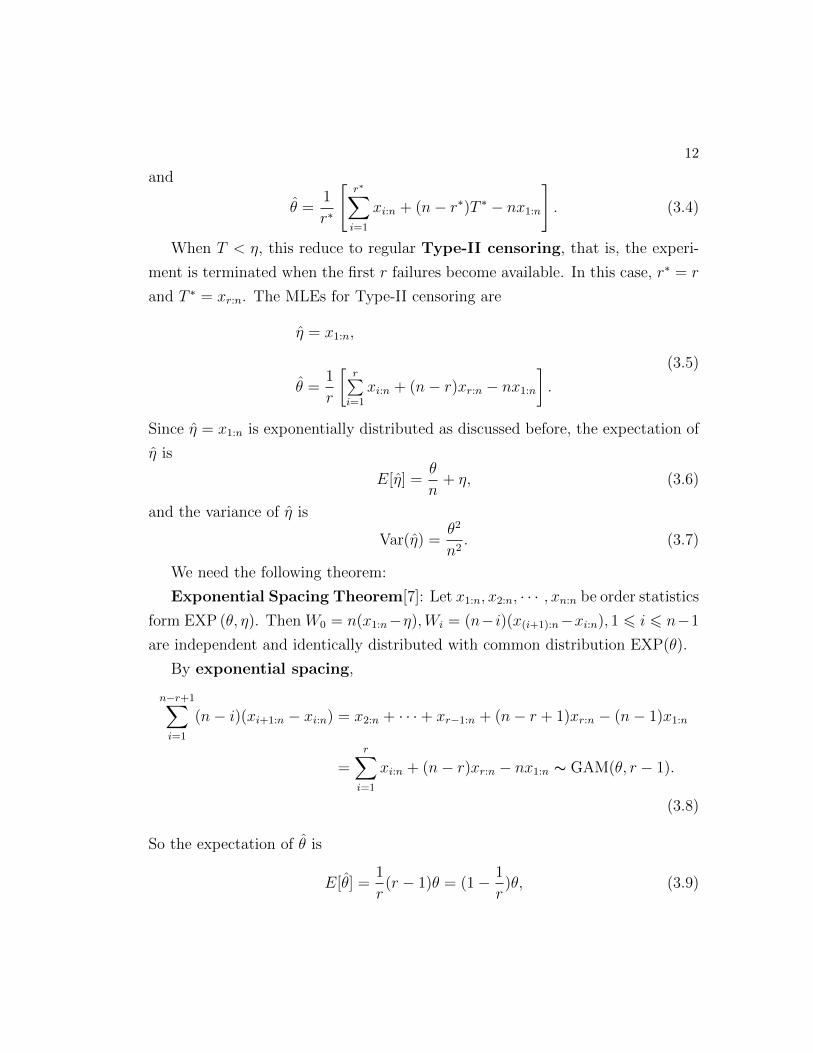
and

θ =1

r∗

[r∗∑i=1

xi:n + (n− r∗)T ∗ − nx1:n

]. (3.4)

When T < η, this reduce to regular Type-II censoring, that is, the experi-

ment is terminated when the first r failures become available. In this case, r∗ = r

and T ∗ = xr:n. The MLEs for Type-II censoring are

η = x1:n,

θ =1

r

[r∑i=1

xi:n + (n− r)xr:n − nx1:n].

(3.5)

Since η = x1:n is exponentially distributed as discussed before, the expectation of

η is

E[η] =θ

n+ η, (3.6)

and the variance of η is

Var(η) =θ2

n2. (3.7)

We need the following theorem:

Exponential Spacing Theorem[7]: Let x1:n, x2:n, · · · , xn:n be order statistics

form EXP (θ, η). Then W0 = n(x1:n−η),Wi = (n−i)(x(i+1):n−xi:n), 1 6 i 6 n−1

are independent and identically distributed with common distribution EXP(θ).

By exponential spacing,

n−r+1∑i=1

(n− i)(xi+1:n − xi:n) = x2:n + · · ·+ xr−1:n + (n− r + 1)xr:n − (n− 1)x1:n

=r∑i=1

xi:n + (n− r)xr:n − nx1:n ∼ GAM(θ, r − 1).

(3.8)

So the expectation of θ is

E[θ] =1

r(r − 1)θ = (1− 1

r)θ, (3.9)

13

the bias of θ is

b(θ) = E[θ]− θ = −1

rθ, (3.10)

and the variance of θ is

Var(θ) =r − 1

r2θ2. (3.11)

The MSE of η is the same as calculated before,

MSE(η) =2θ2

n2. (3.12)

From (3.10), (3.11), the MSE of θ is

MSE(θ) = Var(θ) + [b(θ)]2 =r − 1

r2θ2 + (θ − θ

r− θ)2 =

θ2

r. (3.13)

When T > η,

θ =

1

N

[N∑i=1

xi:n + (n−N)T − nx1:n]

if xr:n < T,

1

r

[r∑i=1

xi:n + (n− r)xr:n − nx1:n]

if xr:n > T.

(3.14)

This result could be found in [8].

3.2 Penalized MLE for Incomplete Data

The regular Type-II hybrid censoring MLE again uses the smallest observation

x1:n to estimate the location parameter η, since the likelihood function is monotone

increasing as a function of η. Again, T is a fixed experimental time, r is a fixed

number of failures, and N is the number of failures that happened before time

T . The experiment ends at time T ∗ = maxxr:n, T. When the experiment ends,

the number of observations r∗ = maxr,N. Again, assume r ≥ 2. Our approach

is to add the penalty multiplier (x1:n − η) in the usual likelihood function so

that the new likelihood function is no longer a monotone function of the location

parameter. The penalized likelihood function of the observed data is given by

L∗(θ, η) = (x1:n − η)n!

(n− r∗)!θr∗e−

1

θ

r∗∑i=1

(xi:n−η)−1

θ(n−r)(T ∗−η)

, x1:n > η. (3.15)

14

Logarithm of the likelihood function is

lnL∗(θ, η) = ln(x1:n − η) + lnn!

(n− r∗)!− r∗ ln θ

− 1

θ

r∗∑i=1

(xi:n − η)− 1

θ(n− r∗)(T ∗ − η), x1:n > η.

By solving the following equations

d(lnL∗(θ, η))

dη= − 1

x1:n−η +r∗

θ+n− r∗

θ= 0,

d(lnL∗(θ, η))

dθ= −r

∗

θ+

r∗∑i=1

(xi:n − η)

θ2+

(n− r∗)(T ∗ − η)

θ2= 0,

we have the penalized MLEs

η∗ =

nr∗x1:n −r∗∑i=1

xi:n − (n− r∗)T ∗

n(r∗ − 1), (3.16)

and

θ∗ = n(x1:n − η∗) =

−nx1:n +r∗∑i=1

xi:n + (n− r∗)T ∗

r∗ − 1. (3.17)

When T < η, this yields to Type-II censoring with r∗ = r and T ∗ = xr:n.

The Type-II censoring MLEs are

η∗ =

nrx1:n −r∑i=1

xi:n − (n− r)xr:n

n(r − 1), (3.18)

and

θ∗ =

−nx1:n +r∑i=1

xi:n + (n− r)xr:n

r − 1. (3.19)

These estimators are the same results as constructed by Epstein and Sobel[7]

before. And they had proved that these estimators are also UMVUE for θ and η.

15

By using (3.8), the expectation of θ∗ is

E[θ∗] =1

(r − 1)(r − 1)θ = θ. (3.20)

From (3.20), θ∗ is unbiased estimator of θ, and the bias is

b(θ∗) = E[θ∗]− θ = 0. (3.21)

The variance of θ∗ is

Var(θ∗) =1

(r − 1)2(r − 1)θ2 =

θ2

r − 1. (3.22)

Note that η∗ = x1:n −θ∗

n, by exponential spacing theorem [7], x1:n and θ∗ are

independent, and the expectation of η∗ is given by

E[η∗] = E[x1:n −θ∗

n] = E[x1:n]− 1

nE[θ∗] =

θ

n+ η − θ

n= η. (3.23)

From (3.23), η∗ is an unbiased estimator of η, and the bias is

b(η∗) = E[η∗]− η = 0. (3.24)

The variance of η∗ is

Var(η∗) = Var(x1:n −θ∗

n) =

θ2

n2+

θ2

n2(r − 1)=

rθ2

n2(r − 1). (3.25)

From (3.21), (3.22), the MSE of θ∗ is

MSE(θ∗) = Var(θ∗) + [b(θ∗)]2 =θ2

r − 1. (3.26)

From (3.24), (3.25), MSE of η∗ is

MSE(η∗) = Var(η∗) + [b(η∗)]2 =rθ2

n2(r − 1). (3.27)

Notice that when r = n, the penalized Type-II censoring MLE has the same

results as penalized MLE for complete data. From (3.12), (3.13), (3.26), (3.27), the

penalized Type-II censoring MLE is consistently better than the regular Type-II

censoring MLE. Again, the penalized method removes the biases completely.

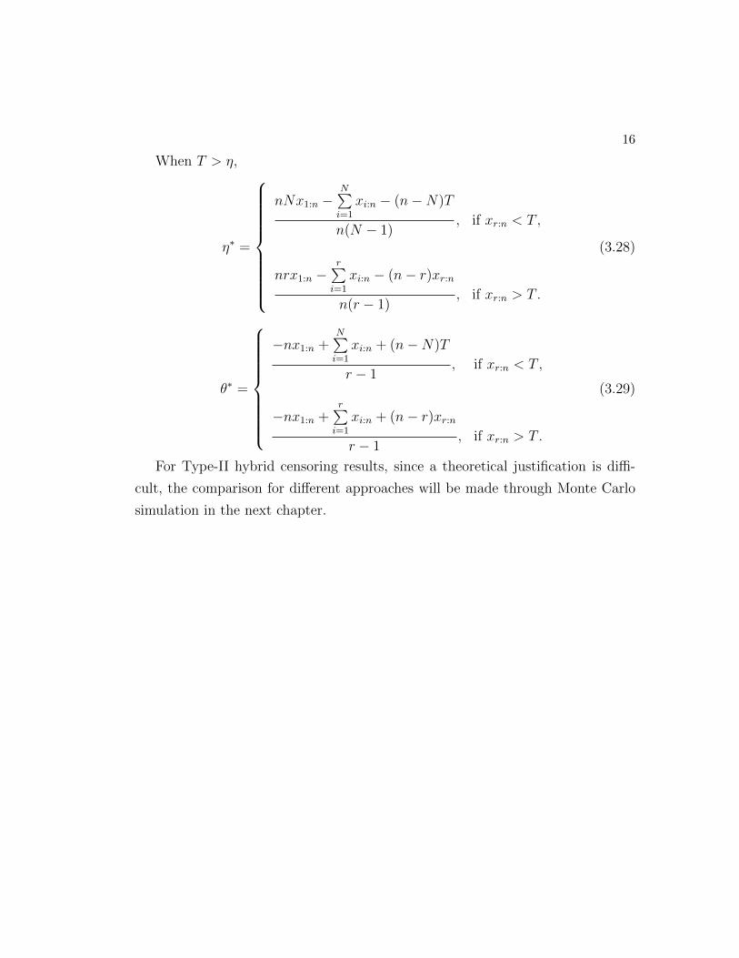
16

When T > η,

η∗ =

nNx1:n −N∑i=1

xi:n − (n−N)T

n(N − 1), if xr:n < T,

nrx1:n −r∑i=1

xi:n − (n− r)xr:n

n(r − 1), if xr:n > T.

(3.28)

θ∗ =

−nx1:n +N∑i=1

xi:n + (n−N)T

r − 1, if xr:n < T,

−nx1:n +r∑i=1

xi:n + (n− r)xr:n

r − 1, if xr:n > T.

(3.29)

For Type-II hybrid censoring results, since a theoretical justification is diffi-

cult, the comparison for different approaches will be made through Monte Carlo

simulation in the next chapter.

Chapter 4

Simulation Results

In this chapter, we demonstrate simulation results for both complete data and

incomplete data with different approaches.

4.1 Simulation for complete data

For a complete data set, we choose the value of the location parameter η to be 0

and scale parameter θ to be 1. We take different values for sample size n: 10, 20,

50, 100. For each sample size, the simulation is repeated 1000 times. The results

of biases and MSEs of regular MLE and penalized MLE are reported in Table 4.1.

In the table, the numbers with parenthesis are MSEs, and the numbers without

parenthesis are biases.

17

18

Table 4.1: The biases and MSEs of estimators for complete data

θ = 1, η = 0 Regular MLE Penalized MLE

n η θ η θ

100.1013 -0.1072 0.0021 -0.0081

(0.0203) (0.0888) (0.0107) (0.0955)

200.0525 -0.0417 0.0021 0.0088

(0.0056) (0.0482) (0.0030) (0.0515)

500.0199 -0.0184 -0.0001 0.0016

(0.0008) (0.0207) (0.0004) (0.0212)

1000.0106 -0.0075 0.0006 0.0026

(0.0002) (0.0099) (0.0001) (0.0101)

From Table 4.1, it is clear that for each sample size n, the penalized MLEs

are better than normal MLEs in terms of bias; the penalized estimators have

strong superiority especially for small n; and MSE(θ∗) is grater than MSE(θ), and

the differences between them become smaller as n increasing ; MSE(η∗) is much

smaller than MSE(η), when n is larger, MSE(η∗) is only half of MSE(η).

19

4.2 Simulation for incomplete data

For incomplete data sets, we choose the values of location η to be 0 and scale

parameter θ to be 1. We take n = 10, r = 2, 5, 8, n = 20, r = 4, 10, 18, n = 50, r =

10, 25, 48, and take different values for T : 1.5, 2.5, 5. Each simulation is repeated

1000 times.

Table 4.2 reports the biases and MSEs of estimators for regular MLE and

penalized MLE, when the total sample size is 10, the predetermined number of

failures are 2, 5, 8, and the predetermined times are 1.5, 2.5, 5. In the table, the

numbers inside parenthesis are MSEs, and the numbers without parenthesis are

biases.

Table 4.2: The biases and MSEs of estimators for Type-II HCS, with n = 10

θ = 1, η = 0 Regular MLE Penalized MLE

T r η θ η θ

1.5

20.1013 -0.0865 -0.0050 0.0637

(0.0203) (0.1230) (0.0115) (0.1945)

50.0966 -0.0739 -0.0113 0.0785

(0.0188) (0.1344) (0.0115) (0.2118)

80.1020 -0.1201 0.0025 -0.0048

(0.0203) (0.1230) (0.0115) (0.1945)

2.5

20.1008 -0.0773 -0.0033 0.0408

(0.0192) (0.1090) (0.0103) (0.1436)

50.0983 -0.0649 -0.0072 0.05487

(0.0193) (0.1054) (0.0113) (0.1431)

80.1005 -0.0911 -0.0017 0.0222

(0.0208) (0.1071) (0.0119) (0.1308)

5

20.1069 -0.0905 0.0057 0.0119

(0.0232) (0.0982) (0.0119) (0.0130)

50.1052 -0.0945 0.0045 0.0076

(0.0215) (0.1047) (0.0118) (0.1202)

80.1020 -0.1007 0.0019 0.0006

(0.0203) (0.1037) (0.0108) (0.1177)

20


penalized MLE, when the total sample size is 20, the fixed number of failures are

4, 10, 18, and the fixed times are 1.5, 2.5, 5. In the table, the numbers inside

parenthesis are MSEs, and the numbers without parenthesis are biases.


θ = 1, η = 0 Normal MLE Penalized MLE

T r η θ η θ

1.5

40.0489 -0.0353 -0.0028 0.0347

(0.0049) (0.0682) (0.0026) (0.0843)

100.0513 -0.0439 0.0001 0.0256

(0.0054) (0.0704) (0.0029) (0.0856)

180.0507 -0.0521 0.0006 0.0009

(0.0050) (0.0587) (0.0026) (0.0627)

2.5

40.0479 -0.04010 -0.0029 0.0153

(0.0045) (0.0541) (0.0023) (0.0609)

100.0498 -0.0463 -0.0007 0.0096

(0.0050) (0.0541) (0.0027) (0.0601)

180.0497 -0.0488 -0.0006 0.0048

(0.0047) (0.0533) (0.0023) (0.0572)

5

40.0526 -0.0406 0.0021 0.0104

(0.0055) (0.0496) (0.0028) (0.0535)

100.0503 -0.0418 -0.0002 0.0092

(0.0049) (0.0496) (0.0024) (0.0535)

180.0517 -0.0525 0.0019 -0.0022

(0.0055) (0.0480) (0.0029) (0.0504)

21


penalized MLE, when the total sample size is 50, the fixed number of failures are

10, 25, 48, and the fixed times are 1.5, 2.5, 5. In the table, the numbers inside

parenthesis are MSEs, and the numbers without parenthesis are biases.


θ = 1, η = 0 Normal MLE Penalized MLE

T r η θ η θ

1.5

100.0199 -0.0069 -0.0005 0.0198

(0.0008) (0.0275) (0.0004) (0.0300)

250.0208 -0.0159 0.0005 0.0106

(0.0009) (0.0259) (0.0005) (0.0279)

480.0203 -0.0243 0.0004 -0.0039

(0.0008) (0.0209) (0.0004) (0.0212)

2.5

100.0200 -0.0164 -0.0002 0.0056

(0.0008) (0.0223) (0.0004) (0.0234)

250.0205 -0.0147 0.0003 0.0074

(0.0008 ) (0.0234) (0.0004) (0.0245)

480.0202 -0.0218 0.0002 -0.0013

(0.0008) (0.0203) (0.0004) (0.0206)

5

100.0188 -0.0242 -0.0011 -0.0041

(0.0007) (0.0202) (0.0004) (0.0205)

250.0194 -0.0163 -0.0007 0.0039

(0.0008) (0.0210) (0.0004) (0.0217)

480.0201 -0.0237 0.0001 -0.0037

(0.0008) (0.0203) (0.0004) (0.0206)

From Table 4.2, Table 4.3 and Table 4.4, for each sample size n, we see that the

penalized MLEs are consistently better than normal MLEs in terms of biases; the

penalized estimators have strong superiority, especially for small n; and MSE(θ∗)

is slightly greater than MSE(θ), the differences between them become smaller with

n increasing; MSE(η∗) is much smaller than MSE(η), about half of MSE(η).

References

[1] A. E. Sarhan (1954). Estimation of the Mean and Standard Deviation by

Order Statistics. The Annals of Mathematical Statistics, Vol. 25, 317-328.

[2] A. Clifford Cohen, Frederick Russell Helm (1973). Estimation in the Expo-

nential Distribution. Technometrics, Vol. 15, 415-418.

[3] Lee J. Bain, Max Engelhardt (1991). Introduction to probability and math-

ematical statistics. Second edition. Duxbury Classic Series.

[4] E. L. Lehmann, George Casella (1998). Theory of Point Estimation. Second

edition. Springer-Verlag, New York.

[5] B. Epstein (1954), Truncated Life Tests in the Exponential Case. The Annals

of Mathematical Statistics, Vol. 25, 555-564.

[6] A. Childs, B. Chandrasekhar, N. Balakrishnan, and D. Kundu (2003). Exact

likelihood inference based on type-I and type-II hybrid censored samples from

the exponential distribution. Annals of the Institute of Statistical Mathemat-

ics, Vol. 55, 319-330.

[7] B. Epstein, M. Sobel (1954). Some theorems relevant to life testing from

an exponential distribution. The Annals of Mathematical Statistics, Vol. 25,

373-381.

[8] A. Ganguly, S. Mitra, D. Samanta, D. Kundu (2012). Exact inference for

the two-parameter exponential distribution under Type-II hybrid censoring.

Journal of Statistical Planning and Inference, Vol 142, 613-625.

22

Appendix A

R code

#Mengjie Zheng Project Simulation

# For complete data

# fix the location to be 0

locate = 0

# fix the scale to be 1

scale = 1

# number of times for repeat

B=1000

#n is total number of observations

set.seed(1234)

for(n in c(10, 20, 30, 50, 100, 1000,10000))

nscale = rep(0, B)

nlocate = rep(0, B)

pscale = rep(0, B)

plocate = rep(0, B)

23

24

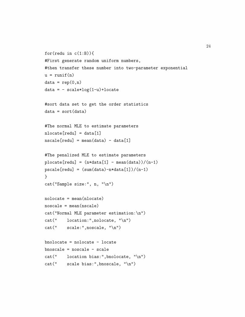
for(redu in c(1:B))

#First generate random uniform numbers,

#then transfer these number into two-parameter exponential

u = runif(n)

data = rep(0,n)

data = - scale*log(1-u)+locate

#sort data set to get the order statistics

data = sort(data)

#The normal MLE to estimate parameters

nlocate[redu] = data[1]

nscale[redu] = mean(data) - data[1]

#The penalized MLE to estimate parameters

plocate[redu] = (n*data[1] - mean(data))/(n-1)

pscale[redu] = (sum(data)-n*data[1])/(n-1)

cat("Sample size:", n, "\n")

nolocate = mean(nlocate)

noscale = mean(nscale)

cat("Normal MLE parameter estimation:\n")

cat(" location:",nolocate, "\n")

cat(" scale:",noscale, "\n")

bnolocate = nolocate - locate

bnoscale = noscale - scale

cat(" location bias:",bnolocate, "\n")

cat(" scale bias:",bnoscale, "\n")

25

nmselocate = var(nlocate)+(mean(nlocate)-locate)*(mean(nlocate)-locate)

nmsescale = var(nscale)+(mean(nscale)-scale)*(mean(nscale)-scale)

cat(" MSE for location:",nmselocate, "\n")

cat(" MSE for scale:",nmsescale, "\n")

pelocate = mean(plocate)

pescale = mean(pscale)

cat("Penalized MLE estimation:\n")

cat(" location:",pelocate, "\n")

cat(" scale:",pescale, "\n")

pbnolocate = pelocate - locate

pbnoscale = pescale - scale

cat(" location bias:",pbnolocate , "\n")

cat(" scale bias:",pbnoscale, "\n")

pmselocate = var(plocate)+(mean(plocate)-locate)*(mean(plocate)-locate)

pmsescale = var(pscale)+(mean(pscale)-scale)*(mean(pscale)-scale)

cat(" MSE for location:",pmselocate, "\n")

cat(" MSE for scale:",pmsescale, "\n")

cat("\n")

#Mengjie Zheng Project Simulation

# For incomplete data

#n is total number of observations

#r is the fixed number of observations

#T is the fixed time

n = 10

26

# fix the location to be 0

locate = 0

# fix the scale to be 1

scale = 1

# number of times for repeat

B=1000

set.seed(1234)

for(n in c(10, 20, 50))

for(r in c(n/5, n/2, n-2))

for(T in c(1.5, 2.5, 5, 20, 100))

nscale = rep(0, B)

nlocate = rep(0, B)

pscale = rep(0, B)

plocate = rep(0, B)

for(redu in c(1:B))

#First generate random uniform numbers,

#then transfer these number into two-parameter exponential

u = runif(n)

data = rep(0,n)

data = - scale*log(1-u)+locate

#sort data set to get the order statistics

data = sort(data)

#Time for the rth observation

timeR = data[r]

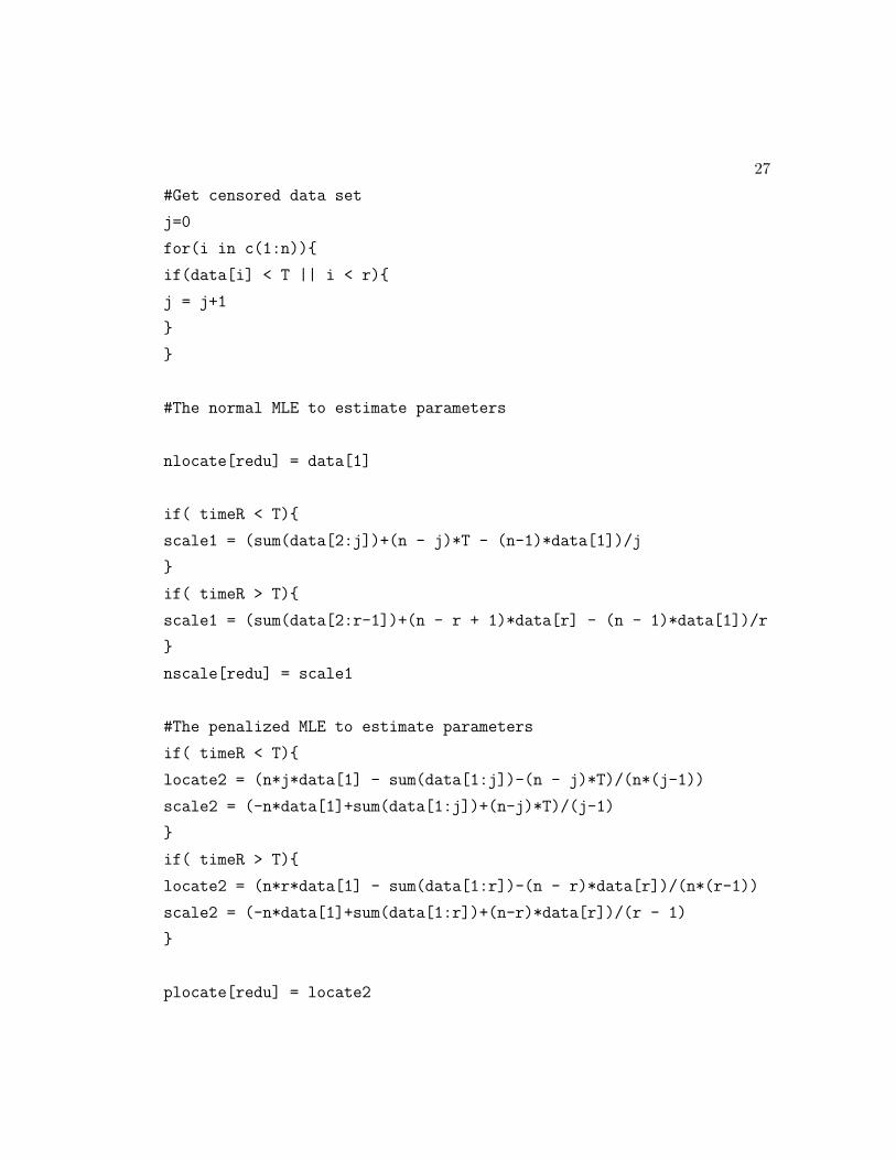
27

#Get censored data set

j=0

for(i in c(1:n))

if(data[i] < T || i < r)

j = j+1

#The normal MLE to estimate parameters

nlocate[redu] = data[1]

if( timeR < T)

scale1 = (sum(data[2:j])+(n - j)*T - (n-1)*data[1])/j

if( timeR > T)

scale1 = (sum(data[2:r-1])+(n - r + 1)*data[r] - (n - 1)*data[1])/r

nscale[redu] = scale1

#The penalized MLE to estimate parameters

if( timeR < T)

locate2 = (n*j*data[1] - sum(data[1:j])-(n - j)*T)/(n*(j-1))

scale2 = (-n*data[1]+sum(data[1:j])+(n-j)*T)/(j-1)

if( timeR > T)

locate2 = (n*r*data[1] - sum(data[1:r])-(n - r)*data[r])/(n*(r-1))

scale2 = (-n*data[1]+sum(data[1:r])+(n-r)*data[r])/(r - 1)

plocate[redu] = locate2

28

pscale[redu] = scale2

cat("Scale:",scale, "\n")

cat("Fixed number:", r, "\n")

cat("Total number:", n, "\n")

cat("Fixed time:", T, "\n")

nolocate = mean(nlocate)

noscale = mean(nscale)

cat("Normal MLE parameter estimation:\n")

cat(" location:",nolocate, "\n")

cat(" scale:",noscale, "\n")

blocation = nolocate - locate

bscale = noscale - scale

cat(" location bias:",blocation, "\n")

cat(" scale bias:",bscale, "\n")

nmselocate = var(nlocate)+(mean(nlocate)-locate)*(mean(nlocate)-locate)

nmsescale = var(nscale)+(mean(nscale)-scale)*(mean(nscale)-scale)

cat(" MSE for location:",nmselocate, "\n")

cat(" MSE for scale:",nmsescale, "\n")

pelocate = mean(plocate)

pescale = mean(pscale)

cat("Penalized MLE estimation:\n")

cat(" location:",pelocate, "\n")

cat(" scale:",pescale, "\n")

29

pblocation = pelocate - locate

pbscale = pescale - scale

cat(" location bias:",pblocation, "\n")

cat(" scale bias:",pbscale, "\n")

pmselocate = var(plocate)+(mean(plocate)-locate)*(mean(plocate)-locate)

pmsescale = var(pscale)+(mean(pscale)-scale)*(mean(pscale)-scale)

cat(" MSE for location:",pmselocate, "\n")

cat(" MSE for scale:",pmsescale, "\n")

cat("\n")

Penalized Maximum Likelihood Estimation of Two … Reports/Technical Reports 2007-/TR... ·...

Documents

Transcript of Penalized Maximum Likelihood Estimation of Two … Reports/Technical Reports 2007-/TR... ·...