PEAKS OVER RANDOM THRESHOLD METHOD- OLOGY · PDF filepeaks over random threshold method-ology...

REVSTAT – Statistical Journal

Volume 4, Number 3, November 2006, 227–247

PEAKS OVER RANDOM THRESHOLD METHOD-

OLOGY FOR TAIL INDEX AND HIGH QUANTILE

ESTIMATION

Authors: Paulo Araujo Santos

– ESGS, Instituto Politecnico de Santarem, [email protected]

M. Isabel Fraga Alves

– CEAUL and DEIO (FCUL), Universidade de Lisboa, [email protected]

M. Ivette Gomes

– CEAUL and DEIO (FCUL), Universidade de Lisboa, [email protected]

Received: May 2006 Accepted: September 2006

Abstract:

• In this paper we present a class of semi-parametric high quantile estimators whichenjoy a desirable property in the presence of linear transformations of the data. Sucha feature is in accordance with the empirical counterpart of the theoretical linearityof a quantile χp: χp(δX + λ) = δχp(X) + λ, for any real λ and positive δ. This classof estimators is based on the sample of excesses over a random threshold, originatingwhat we denominate PORT (Peaks Over Random Threshold) methodology. We proveconsistency and asymptotic normality of two high quantile estimators in this class,associated with the PORT -estimators for the tail index. The exact performance ofthe new tail index and quantile PORT -estimators is compared with the original semi-parametric estimators, through a simulation study.

Key-Words:

• heavy tails; high quantiles; semi-parametric estimation; linear property; sample of

excesses.

AMS Subject Classification:

• 62G32, 62E20.

228 Paulo Araujo Santos, M. Isabel Fraga Alves and M. Ivette Gomes

PORT Methodology in Heavy Tails 229

1. INTRODUCTION

In this paper we deal with semi-parametric estimators of the tail index γ

and high quantiles χp, which enjoy desirable properties in the presence of linear

transformations of the available data. We recall that a high quantile is a value

exceeded with a small probability. Formally, we denote by F the heavy-tailed

distribution function (d.f.) of a random variable (r.v.) X, the common d.f. of the

i.i.d. sample X := {Xi}ni=1, for which the high quantile

(1.1) χp(X) := F←(1 − p) , p = pn→ 0, as n→∞ , n pn → c ≥ 0 ,

has to be estimated. Here F←(t) := inf{x : F (x) ≥ t} denotes the generalized

inverse function of F .

We consider estimators based on the k + 1 top order statistics (o.s.),

Xn:n ≥ ··· ≥ Xn−k:n, where Xn−k:n is an intermediate o.s., i.e., k is an inter-

mediate sequence of integers such that

(1.2) k = kn → ∞ , kn/n → 0, as n → ∞ .

We assume that we are working in a context of heavy tails, i.e., γ > 0 in the

extreme value distribution

(1.3) Gγ(x) =

{exp{−(1 + γ x)−1/γ

}, 1 + γ x > 0, γ 6= 0

exp(−e−x

), x ∈ R, γ = 0 ,

the non-degenerate d.f. to which the maximum Xn:n is attracted, after a suitable

linear normalization. When this happens we say that the d.f. F is in the Frechet

domain of attraction and we write F ∈ D(Gγ)γ>0.

The paper is developed under the first order regular variation condition,

which allows the extension of the empirical d.f. beyond the range of the available

data, assuming a polynomial decay of the tail. This condition can be expressed

by

(1.4) F ∈ D(Gγ)γ>0 iff F := 1−F ∈ RV−1/γ iff U ∈ RVγ ,

where U is the quantile function defined as U(t) := F←(1−1/t), t≥1; the nota-

tion RVα stands for the class of regularly functions at infinity with index of regular

variation α, i.e., positive measurable functions h such that limt→∞

h(tx)/h(t) = xα,

for all x > 0.

It is interesting to note that the p-quantile can be expressed as χpn =

U(1/pn).


To get asymptotic normality of estimators of parameters of extreme events,

it is usual to assume the following extra second regular variation condition, that

involves a non-positive parameter ρ:

(1.5) limt→∞

U(tx)/U(t) − xγ

A(t)= xγ xρ − 1

ρ,

for all x > 0, where A is a suitably chosen function of constant sign near infinity.

Then, |A| ∈ RVρ and ρ is called the second order parameter (Geluk and de Haan,

1987). For the strict Pareto model, with tail function F (x) = (x/C)−1/γ and

quantile function U(t)=Ctγ , U(tx)/U(t) − xγ ≡ 0. We then consider that (1.5)

holds with A(t) ≡ 0.

More restrictively, we might consider that F belonged to the wide class of

Hall [11], that is, the associated quantile function U satisfies

(1.6) U(t) = Ctγ(1+Dtρ +o(tρ)

), ρ<0, C >0, D∈R, as t→∞ ,

or equivalently, (1.5) holds, with A(t)=Dρtρ. The strict Pareto model appears

when both D and the remainder term o(tρ) are null.

Returning to the problem of high quantile estimation, we recall the classical

semi-parametric Weissman-type estimator of χpn (Weissman, 1978),

(1.7) χpn = χpn(X) = Xn−kn:n

(kn

npn

)γn

,

with γn = γn(X) some consistent estimator of the tail parameter γ.

In the classical approach one considers for γn the well known Hill estimator

(Hill, 1975),

(1.8) γHn = γH

n (X) =1

kn

kn∑

j=1

logXn−j+1:n

Xn−kn:n,

or the Moment estimator (Dekkers et al., 1989),

(1.9) γMn = γM

n (X) = M (1)n + 1 − 1

2

{1 −

(M

(1)n

)2

M(2)n

}−1

,

with M(r)n , the r-Moment of the log-excesses, defined by

(1.10) M (r)n = M (r)

n (X) =1

kn

kn∑

j=1

(log

Xn−j+1:n

Xn−kn:n

)r

, r = 1, 2 .

We use the following notation:

(1.11) χHpn

= Xn−kn:n

(kn

npn

)γHn

, χMpn

= Xn−kn:n

(kn

npn

)γMn

.


Finally, we explain the question that motivated this paper. It is well known

that scale transformations to the data do not interfere with the stochastic be-

haviour of the tail index estimators (1.8) and (1.9), i.e., we can say that they

enjoy scale invariance. The incorporation of (1.8) or (1.9) in the Weissman-type

estimator in (1.7), allows us to obtain the following desirable exact property for

quantile estimators: for any real positive δ,

(1.12) χpn(δX) = δXn−kn:n

(kn

npn

)γn

= δ χpn(X) .

But we want a similar linear property in the case of location transformations to

the data, Zj :=Xj +λ, j =1, ..., n, for any real λ. That is, our main goal is that,

for the transformed data Z := {Zj}nj=1, the quantile estimator satisfies

(1.13) χpn(Z) = χpn(X) + λ .

Altogether, this represents the empirical counterpart of the following theoretical

linear property for quantiles,

(1.14) χp(δX +λ) = δχp(X) + λ , for any real λ and real positive δ .

Here we present a class of high quantile-estimators for which (1.12) and (1.13)

hold exactly, pursuing the empirical counterpart of the theoretical linear property

(1.14). For a simple modification of (1.7) that enjoys (1.13) approximately, see

Fraga Alves and Araujo Santos (2004). For the use of reduced bias tail index

estimation in high quantile estimation for heavy tails, see Gomes and Figueiredo

(2003), Matthys and Beirlant (2003) and Gomes and Pestana (2005), where the

second order reduced bias tail index estimator in Caeiro et al. (2005) is used for

the estimation of the Value at Risk.

1.1. The class of high quantile estimators under study

The class of estimators suggested here is function of a sample of excesses

over a random threshold Xnq :n,

(1.15) X(q) :=(Xn:n−Xnq :n, Xn−1:n−Xnq :n, ..., Xnq+1:n−Xnq :n

),

where nq := [nq]+1, with:

• 0<q<1, for d.f.’s with finite or infinite left endpoint xF := inf{x : F (x)>0}(the random threshold is an empirical quantile);

• q = 0, for d.f.’s with finite left endpoint xF (the random threshold is the

minimum).


A statistical inference method based on the sample of excesses X(q) defined in

(1.15) will be called a PORT -methodology, with PORT standing forPeaks Over

Random Threshold. We propose the following PORT-Weissman estimators:

(1.16) χ(q)pn

= (Xn−kn:n−Xnq :n)

(kn

npn

)γ(q)n

+ Xnq :n ,

where γ(q)n is any consistent estimator of the tail parameter γ, made location/scale

invariant by using the transformed sample X(q). Indeed, the incorporation in the

Adapted-Weissman estimator in (1.16), of tail index estimators, as function of

the sample of excesses, allows us to obtain exactly the linear property (1.13).

1.2. Shifts in a Pareto model

To illustrate the behaviour of the new quantile estimators in (1.16), we

shall first consider a parent X from a Pareto(γ, λ, δ),

(1.17) Fγ,λ,δ(z) = 1 −(

z − λ

δ

)−1/γ

, z > λ+δ, δ > 0 ,

with λ = 0 and γ = δ = 1. Let us assume that we want to estimate an upper

p = pn = 1n -quantile in a sample of size n = 500. Then, we want to estimate

the parameter χp(X) = 500. If we induce a shift λ = 100 to our data, we would

obviously like our estimates to approach χp(X+100) = 600.

In Figure 1 we plot, for the Pareto(λ, 1, 1) parents, with λ = 0 and λ = 100

and for q = 0 in (1.15), the simulated mean values of the Weissman and PORT-

Weissman quantile estimators based on the Hill, denoted χHp and χ

H(q)p , respec-

tively. These mean values are based on N = 500 replications, for each value k,

5≤ k ≤ 500, from the above mentioned models.

Similarly to the Hill horror plots (Resnick, 1997), associated to slowly vary-

ing functions LU(t) = t−γ U(t), we also obtain here Weissman–Hill horror plots

whenever we induce a shift in the simple standard Pareto model. Indeed, for

a standard Pareto model (λ = 0 in (1.17)), Weissman type estimators in (1.7)

perform reasonably well, with γn = γHn . However, a small shift in the data may

lead to disastrous results, even in this simple and specific case. For the PORT-

Weissman estimates, the shift in the quantile estimates is equal to the shift

induced in the data, a sensible property of quantile estimates. Figure 1 also illus-

trates how serious can be the consequences to the sample paths of the classical

high quantile estimators, when we induce a shift in the data, as suggested in

Drees (2003). We may indeed be led to dangerous misleading conclusions, like

a systematic underestimation, for instance, mainly due to “stable zones” far away

of the target quantile to be estimated.


Figure 1: Mean values of χHpn

and χH(0)pn

, pn = 0.002 for samples of size n=500from a Pareto(1, 0, 1) parent (target quantile χpn

= 500) and from thePareto(1, 100, 1) (target quantile χpn

= 600).

1.3. Scope of the paper

As far as we know, no systematic study has been done concerning asymp-

totic and exact properties of semi-parametric methodologies for tail index and

high quantile estimation, using the transformed sample in (1.15). Somehow re-

lated with this subject, Gomes and Oliveira (2003), in a context of regularly

varying tails, suggested a simple generalization of the classical Hill estimator

associated to artificially shifted data. The shift imposed to the data is determin-

istic, with the aim of reducing the main component of the bias of Hill’s estimator,

getting thus estimates with stable sample paths around the target value. A pre-

liminary study has also been carried out, by the same authors, replacing the

artificial deterministic shift by a random shift, which in practice represents a

transformation of the original data through the subtraction of the smallest ob-

servation, added by one, whenever we are aware that the underlying heavy-tailed

model has a finite left endpoint.

With the purpose of tail index and high quantile estimation there is, in our

opinion, a gap in the literature regarding classical semi-parametric estimation

methodologies adapted for shifted data, the main topic of this paper.

In Section 2, we derive asymptotic properties for the adapted Hill and

Moment estimators, as functions of the sample of excesses (1.15). In Section

3, we propose two estimators for χp that belong to the class (1.16) and prove

their asymptotic normality. In Section 4, and through simulation experiments,

we compare the performance of the new estimators with the classical ones.

Finally, in Section 5, we draw some concluding remarks.


2. TAIL INDEX PORT-ESTIMATORS

For the classical Hill and Moment estimators, we know that for any interme-

diate sequence k as in (1.2) and under the validity of the second order condition

in (1.5),

γHn

d= γ +

γ√k

PHk +

A(n/k)

1−ρ

(1 + op(1)

)(2.1)

and

γMn

d= γ +

√γ2 +1√

kPM

k +

(γ(1−ρ) + ρ

)A(n/k)

γ(1−ρ)2(1 + op(1)

),(2.2)

where PHk and PM

k are asymptotically standard normal r.v.’s.

In this section we present asymptotic results for the classical Hill estimator

in (1.8) and the Moment estimator in (1.9), both based on the sample of excesses

X(q) in (1.15), which will be denoted respectively, by

(2.3) γH(q)n := γH

n

(X(q)

)and γM(q)

n := γMn

(X(q)

), 0≤ q < 1 .

In the following, χ∗q denotes the q-quantile of F : F (χ∗q) = q (by convention

χ∗0 := xF ), so that

Xnq :np−→ χ∗q , as n→∞ , for 0≤ q < 1 .

For the estimators in (2.3) we have the asymptotic distributional representations

expressed in Theorem 2.1.

Theorem 2.1 (PORT-Hill and PORT-Moment). For any intermediate

sequence k as in (1.2), under the validity of the second order condition in (1.5),

for any real q, 0 ≤ q < 1, and with T generally denoting either H or M , the

asymptotic distributional representation

(2.4) γT (q)n

d= γ +

σT√k

P Tk +

(c

TA(n/k) + d

T

χ∗qU(n/k)

)(1 + op(1)

)

holds, where P Tk is an asymptotically standard normal r.v.,

σ2H

:= γ2 , cH

:=1

1−ρ, d

H:=

γ

γ +1,(2.5)

σ2

M:= γ2 +1 , c

M:=

γ(1−ρ) + ρ

γ(1−ρ)2and d

M:=

(γ

γ +1

)2

.(2.6)


Remark 2.1. Notice that σ2M

= σ2H

+1, cM

= cH

+ ργ(1−ρ)2

and dM

= (dH)2.

Consequently, σM

> σH

, cM≤ c

Hand d

M< d

H.

The proof of Theorem 2.1 relies on the the following Lemmas 2.1 and 2.2.

Lemma 2.1. Let F be the d.f. of X, and assume that the associated

U -quantile function satisfies the second order condition (1.5). Consider a deter-

ministic shift transformation to X, defining the r.v. Xq := X − χ∗q with d.f.

Fq(x)=F (x)+χ∗q and associated Uq-quantile function given by Uq(t) :=F←q (1−1/t)

= U(t)−χ∗q .

Then Uq satisfies a second order condition similar to (1.5), that is

(2.7) limt→∞

Uq(tx)/Uq(t) − xγ

Aq(t)= xγ

(xρq − 1

ρq

), for x > 0, ρq ≤ 0 ,

with

(2.8)(Aq(t), ρq

):=

(A(t) , ρ

)if ρ >−γ ;

(A(t)+

γχ∗qU(t)

, −γ

)if ρ =−γ ;

(γχ∗qU(t)

, −γ

)if ρ <−γ .

Proof: Under (1.5), for x > 0,

Uq(tx)

Uq(t)=

U(tx) − χ∗qU(t) − χ∗q

=U(tx)

U(t)

{1 − χ∗q /U(tx)

1 − χ∗q /U(t)

}

=U(tx)

U(t)

{1 + χ∗q

1/U(t) − 1/U(tx)

1 − χ∗q /U(t)

}

=U(tx)

U(t)

{1 +

χ∗qU(t)

[1− U(t)

U(tx)

] (1+ o(1)

)}

= xγ

{1 +

xρ−1

ρA(t)

(1+ o(1)

)}{

1 +γχ∗qU(t)

x−γ −1

−γ

(1+ o(1)

)}

= xγ

{1 +

xρ−1

ρA(t) +

γχ∗qU(t)

x−γ −1

−γ+ o(A(t)

)+ o(1/U(t)

)}

.

Then Uq satisfies (2.7), for Aq and ρq defined in (2.8) and the result follows.


Lemma 2.2. Denote by M(r,q)n the M

(r)n statistics in (1.10), as functions

of the transformed sample X(q), 0≤ q < 1 in (1.15); that is,

M (r,q)n := M (r)

n

(X(q)

)=

1

k

k∑

j=1

(log

Xn−j+1:n− Xnq :n

Xn−k:n− Xnq :n

)r

, r = 1, 2 .

Then, for any intermediate sequence k as in (1.2), under the validity of the second

order condition in (1.5) and for any real q, 0≤ q < 1,

M (r,q)n − 1

k

k∑

j=1

(log

Xn−j+1:n− χ∗qXn−k:n− χ∗q

)r

= op

(1

U(n/k)

), r = 1, 2 .

Proof: We will consider r = 1. Using the first order approximation

ln(1+ x) ∼ x, as x → 0, together with the fact that Xnq :n = χ∗q(1+ op(1)

),

we will have successively

M (1,q)n − 1

k

k∑

j=1

logXn−j+1:n− χ∗qXn−k:n− χ∗q

=

=1

k

k∑

j=1

logXn−j+1:n− Xnq :n

Xn−k:n− Xnq :n− log

Xn−j+1:n− χ∗qXn−k:n− χ∗q

=1

k

k∑

j=1

log1 − Xnq :n/Xn−j+1:n

1 − Xnq :n/Xn−k:n− log

1 − χ∗q /Xn−j+1:n

1 − χ∗q /Xn−k:n

=1

k

k∑

j=1

(Xnq :n

Xn−k:n− Xnq :n

Xn−j+1:n+

χ∗qXn−j+1:n

−χ∗q

Xn−k:n

)(1+ op(1)

)

=Xnq :n− χ∗q

Xn−k:n

1

k

k∑

j=1

(1− Xn−k:n

Xn−j+1:n

)(1+ op(1)

)

=op(1)

Xn−k:n

1

k

k∑

j=1

(1− Xn−k:n

Xn−j+1:n

)(1+ op(1)

).

Denote by {Yj}kj=1 i.i.d. Y standard Pareto r.v.’s, with d.f. FY (y) = 1−y−1,

for y > 1 and {Yj:k}kj=1 the associated o.s.’s.

Since Xn−k:nd= U(Yn−k:n), with Yn−k:n the (n−k)-th o.s. associated to an

i.i.d. standard Pareto sample of size n and(

kn

)Yn−k:n

p−→ 1, for any intermediate

sequence k, thenXn−k:n

U(n/k)

p−→ 1; this together with the fact that

{Yn−j+1:n

Yn−k:n

}k

j=1

d={

Yk−j+1:k

}k

j=1


allow us to write

M (1,q)n − 1

k

k∑

j=1


=

=op(1)

U(Yn−k:n)

1

k

k∑

j=1

1 − U(Yn−k:n)

U(

Yn−j+1:n

Yn−k:nYn−k:n

)

(1+ op(1))

=1

k

k∑

j=1

(1− Y −γ

k−j+1:k

)op

(1

U(n/k)

)(1+ op(1)

)

=1

k

k∑

j=1

(1− Y −γ

j

)op

(1

U(n/k)

)(1+ op(1)

).

Now E[Y −γ

]= 1

γ+1 and by the weak law of large numbers we obtain

M (1,q)n − 1

k

k∑

j=1


=

=γ

γ +1

(1+ op

(1/√

k))

op

(1

U(n/k)

)

= op

(1

U(n/k)

).

For r = 2 steps similar to the previous ones lead us to the result.

Remark 2.2. Note that if q ∈ (0, 1), Xnq :n− χ∗q = Op(1/√

n) and for

r = 1, 2,√

k[M

(r,q)n − 1

k

∑kj=1

{log

Xn−j+1:n−χ∗

q

Xn−k:n−χ∗

q

}r ]= Op

(√k/n 1

U(n/k)

)= op(1)

holds.

Proof of Theorem 2.1: Taking into account Lemma 2.2

γH(q)n =

1

k

k∑

j=1


+ op

(1

U(n/k)

).

Now, considering the result in Lemma 2.1 and representation (2.1) adapted for

the deterministic shift data from Xq := X − χ∗q model, we obtain the following

representation for PORT -Hill estimator

γH(q)n

d= γ +

γ√k

PHk +

Aq(n/k)

1−ρq

(1+ op(1)

)+ op

(1

U(n/k)

),

with Aq(t) provided in (2.8), and the result (2.4) follows with T = H.


Similarly, considering Lemmas 2.1 and 2.2 and the representation (2.2)

adapted for the deterministic shift data from Xq := X− χ∗q model, we obtain for

the PORT -Moment estimator the representation

γM(q)n

d= γ +

√γ2+1√

kPM

k +

(γ(1−ρq)+ρq

)Aq(n/k)

γ(1−ρq)2

(1+op(1)

)+op

(1

U(n/k)

),

and result (2.4) follows with T = M .

Remark 2.3. Note that if we induce a deterministic shift λ to data X

from a model F =: F0, i.e., if we work with the new model Fλ(x) := F0(x−λ), the

associated U -quantile function changes to Uλ(t) = λ + δU0(t). Then, as expected,

(2.4) holds whenever we replace γH(q)n by γH

n |λ (the Hill estimator associated

with the shifted population with shift λ) provided that we replace χ∗q by −λ.

This topic has been handled in Gomes and Oliveira (2003), where the shift λ is

regarded as a tuning parameter of the statistical procedure that leads to the tail

index estimates. The same comments apply to the classical Moment estimator.

Corollary 2.1. For the strict Pareto model, i.e., the model in (1.17) with

λ = 0 and γ = δ = 1, the distributional representations (2.4) holds with A(t)

replaced by 0.

Under the conditions of Theorems 2.1 and with the notations defined in

(2.5) and (2.6), the following results hold:

Corollary 2.2. Let µ1 and µ2 be finite constants and let T generically

denote either H or M .

i) For γ > −ρ,

γT (q)n

d= γ +

σT√k

P Tk + c

TA(n/k)

(1 + op(1)

).

If√

k A(n/k) → µ1, then

√k(γT (q)

n − γ)

d−→n→∞

Normal(µ1 c

T, σ2

T

).

ii) For γ < −ρ,

γT (q)n

d= γ +

σT√k

P Tk + d

T

χ∗qU(n/k)

(1+ op(1)

).

If√

k/U(n/k) → µ2, then

√k(γT (q)

n − γ)

d−→n→∞

Normal(µ2 d

Tχ∗q , σ2

T

).


iii) For γ = −ρ,

γT (q)n

d= γ +

σT√k

P Tk +

[c

TA(n/k) + d

T

χ∗qU(n/k)

] (1+ op(1)

).

If√

k A(n/k) → µ1 and√

k/U(n/k) → µ2, then

√k(γT (q)

n − γ)

d−→n→∞

Normal(µ1 c

T+ µ2 d

Tχ∗q , σ2

T

).

3. HIGH QUANTILE PORT-ESTIMATORS

On the basis of (1.16), we shall now consider the following estimators of χpn ,

functions of the sample of excesses over Xnq :n, i.e., of the sample X(q) in (1.15):

χH(q)pn

:=(Xn−kn:n− Xnq :n

)( kn

npn

)γH(q)n

+ Xnq :n , 0≤ q < 1 ,(3.1)

χM(q)pn

:=(Xn−kn:n− Xnq :n

)( kn

npn

)γM(q)n

+ Xnq :n , 0≤ q < 1 .(3.2)

For these estimators we have the asymptotic distributional representations pre-

sented in Theorem 3.1.

Theorem 3.1. In Hall’s class (1.6), for intermediate sequences kn that

satisfy

(3.3) log (npn)/√

kn → 0 , as n→∞ ,

with pn such that (1.1) holds, then, with T denoting either H or M , (cH

, dH

, σH

)

and (cM

, dM

, σM

) defined in (2.5) and (2.6), respectively, and for any real q,

0 ≤ q < 1,

√kn

σT log(kn/(npn)

)(

χT (q)pn

χpn

−1

)= P T

k +√

kn

(c

TA(n/k)+d

T

χ∗qU(n/k)

)(1+op(1)

),

where P Tk is an asymptotically standard normal r.v.

Proof: From now on, we denote an := kn

npn. With the underlying condi-

tions in (1.1), an tends to infinity, as n→∞, and the quantile to be estimated

can be expressed as

χpn = U

(1

pn

)= U

(nan

kn

).

We will present the proof for T = H, since for T = M the proof follows

the same steps.


First notice that

χH(q)pn

=(Xn−kn:n− Xnq :n

)aγ

H(q)n

n + Xnq :n

= Xn−kn:n

[(1 − Xnq :n

Xn−kn:n

)aγ

H(q)n

n +Xnq :n

Xn−kn:n

].

Now, since Xnq :np−→χ∗q , we have

Xnq :n

Xn−kn:n= op(1). Then

χH(q)pn

= Xn−kn:n

[aγ

H(q)n

n

(1+ op(1)

)],

which means that the proposed estimator χH(q)pn is asymptotically equivalent to

the Weissman type estimator (1.7), whenever we use the consistent estimator

γn ≡ γH(q)n .

Consider now a convenient representation for the difference,

χH(q)pn

− χpn = Xn−kn:n

{aγ

H(q)n

n − aγH(q)n

n

(Xnq :n

Xn−kn:n

)+

Xnq :n

Xn−kn:n− χpn

Xn−kn:n

},

and recall that we may write

χpn

Xn−kn:n=

U(

nkn

an

)

U(

nkn

)U(

nkn

)

U(Yn−kn:n).

According to (1.5), for ρ < 0, U(

nkn

an

)/U(

nkn

)= aγ

n

(1−A(n/kn)/ρ

) (1+op(1)

).

Considering that for the estimator γH(q)n , the representation (2.4) holds,

we get successively, for sequences kn that verify (3.3),

aγH(q)n

n = aγn

(1+ log an

(γH(q)

n − γ)) (

1+ op(1))

and

χH(q)pn

− χpn =

= aγn Xn−kn:n

{1+ log an

(γH(q)

n −γ)(

1+op(1))−(1−A(n/kn)/ρ

)(1+op(1)

)}

= aγn Xn−kn:n

{log an

(γH(q)

n −γ)

+ A(n/kn)/ρ

}(1+op(1)

).

Now, we consider the following representation for intermediate statistics, proved

in Ferreira et al. (2003),

(3.4) Xn−kn:nd= U

(n

kn

)(1 +

γBk√kn

+ op

(1√kn

)+ op

(A(n/kn)

)),

with Bk an asymptotically standard normal r.v.


Using (2.4) and (3.4), we may write

χH(q)pn

− χpn = U

(n

kn

)aγ

n

(1+ Op

(1/√

kn

)){Wn + A

( n

kn

)/ρ

}(1+ op(1)

),

where

Wn = log an

(γH(q)

n − γ)

= log an

(σH√kn

PHk +

(c

HA(n/k) + d

H

χ∗qU(n/k)

)(1+ op(1)

))

,

with PHk independent of the random sequence Bk in (3.4).

Consequently,

χH(q)pn − χpn

aγn U(

nkn

) ={Wn + A(n/k)/ρ

} (1+ op(1)

)

and

√kn

σH log an

(χ

H(q)pn

χpn

− 1

)= PH

k +√

kn

(c

HA(n/k) + d

H

χ∗qU(n/k)

)(1+ op(1)

).

The following result is a direct consequence of Corollary 2.2 and Theorem 3.1.

Corollary 3.1. Under the same conditions of Theorem 3.1, then, with

T replaced by H or M , and (cH

, dH

, σH) and (c

M, d

M, σ

M) defined in (2.5) and (2.6),

respectively, the following results hold.

i) For γ > −ρ,

√kn

σT

log(kn/(npn)

)(

χT (q)pn

χpn

−1

)= P T

k +√

kn

(c

TA(n/k)

) (1+ op(1)

),

If√

kn A(n/kn) → µ1, finite, as n→∞, then the mean value is µ1 cT

.

ii) For γ < −ρ,

√kn

σT

log(kn/(npn)

)(

χT (q)pn

χpn

−1

)= P T

k +√

kn

(d

T

χ∗qU(n/kn)

)(1+ op(1)

),

If√

kn/U(n/kn)→µ2, finite, as n→∞, then the mean values is µ2dTχ∗q .


iii) For ρ = −γ,

√kn

σT

log(kn/(npn)

)(

χT (q)pn

χpn

−1

)=

= P Tk +

√kn

(c

TA(n/k) + d

T

χ∗qU(n/kn)

)(1+ op(1)

),

If√

kn A(n/kn) → µ1, finite, and√

kn/U(n/kn) → µ2, finite, as n→∞,

then the mean value is µ1 cT

+ µ2 dTχ∗q .

4. SIMULATIONS

Here, we compare the finite sample behavior of the proposed high quantile

estimators χH(q)pn in (3.1) and χ

M(q)pn in (3.2) with the classical semi-parametric

estimators χHpn

and χMpn

in (1.11). We have generated N = 200 independent repli-

cates of sample size n = 1000 from the following models:

• Burr Model: X ⌢ Burr(γ, ρ), γ = 1, ρ =−2,−0.5, with d.f.

F (x) = 1 −(1+ x−ρ/γ

)1/ρ, x ≥ 0 .

• Cauchy Model: X ⌢ Cauchy , γ = 1, ρ =−2, with d.f.

F (x) =1

2+

1

πarctang x , x ∈ R .

At a first stage, we generate samples from the standard models F0 := F . At a

second stage, we introduce a positive shift λ = χ0.01, i.e., a new location chosen

in a comparable basis as the percentile 99% of the starting point distribution F0.

This defines a new model Fλ(x) := F0(x−λ) from the same family.

We estimate the high quantile χ0.001, for each model F0 or Fλ from the

referred Burr and Cauchy families, and we present patterns of Mean Values and

Root of Mean Squared Errors, plotted against k = 6, ..., 800.

The simulations illustrate the dramatic disturbance on the behavior of the

classical quantile estimators in (1.11), when a shift is introduced. We, again,

enhance that the flat stable zones achieved with these estimators, in the presence

of shifts, could lead us to dangerous misleading conclusions, unless we are aware

of the suitable threshold k or of specific properties of the underlying model.


0 200 400 600 800

010

0020

0030

0040

00

k

χp

H(0)

χp

M(0)

χp

M

χp

H

0 200 400 600 800

020

0040

0060

0080

0010

000

k

χp

H(0)

χp

M(0)χp

M

χp

H

Figure 2: Mean values (left) and root mean squared errors (right), of χH(0)pn

,

χM(0)pn

, χHpn

and χMpn

, for a sample size n = 1000, from a Burr modelwith γ = 1, ρ =−2 and λ = 0 (target quantile χ0.001 = 1000).

0 200 400 600 800

010

0020

0030

0040

00

k

χp

H(0)

χp

M(0)

χp

M

χp

H

0 200 400 600 800

020

0040

0060

0080

0010

000

k

χp

H(0)

χp

M(0)

χp

M

χp

H


,

χM(0)pn

, χHpn

and χMpn

, for a sample size n = 1000, from a Burr modelwith γ = 1, ρ =−2 and λ = 99.99 (target quantile χ0.001 = 1099.99).


0 200 400 600 800

010

0020

0030

0040

00

k

χp

H(0)

χp

M(0)

χp

M

χp

H

0 200 400 600 800

020

0040

0060

0080

0010

000

k

χp

H(0)

χp

M(0)

χp

M

χp

H


,

χM(0)pn

, χHpn

and χMpn

, for a sample size n = 1000, from a Burr modelwith γ = 1, ρ =−0.5 and λ = 0 (target quantile χ0.001 = 937.731).

0 200 400 600 800

010

0020

0030

0040

00

k

χp

H(0)

χp

M(0)

χp

M

χp

H

0 200 400 600 800

020

0040

0060

0080

0010

000

k

χp

H(0)

χp

M(0)

χp

M

χp

H


,

χM(0)pn

, χHpn

and χMpn

, for a sample size n = 1000, from a Burr modelwith γ = 1, ρ =−0.5 and λ = 81.023 (target quantile χ0.001 = 1018.754).


0 100 200 300 400

050

010

0015

00

k

χp

H(0.5)

χp

M(0.5)

χp

M

χp

H

0 100 200 300 400

010

0020

0030

0040

0050

00

k

χp

H(0.5)

χp

M(0.5)

χp

M

χp

H

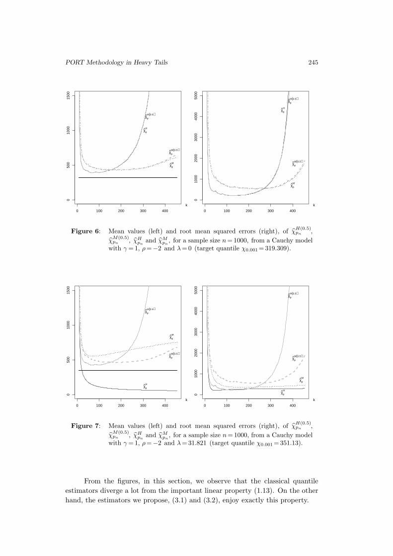
Figure 6: Mean values (left) and root mean squared errors (right), of χH(0.5)pn

,

χM(0.5)pn

, χHpn

and χMpn

, for a sample size n = 1000, from a Cauchy modelwith γ = 1, ρ =−2 and λ = 0 (target quantile χ0.001 = 319.309).

0 100 200 300 400

050

010

0015

00

k

χp

H(0.5)

χp

M(0.5)

χp

M

χp

H

0 100 200 300 400

010

0020

0030

0040

0050

00

k

χp

H(0.5)

χp

M(0.5)

χp

M

χp

H

Figure 7: Mean values (left) and root mean squared errors (right), of χH(0.5)pn

,

χM(0.5)pn

, χHpn

and χMpn

, for a sample size n = 1000, from a Cauchy modelwith γ = 1, ρ =−2 and λ = 31.821 (target quantile χ0.001 = 351.13).

From the figures, in this section, we observe that the classical quantile

estimators diverge a lot from the important linear property (1.13). On the other

hand, the estimators we propose, (3.1) and (3.2), enjoy exactly this property.


5. CONCLUDING REMARKS

• The PORT tail index and quantile estimators, based on the sample of

excesses, X(q), in (1.15), provide us with interesting classes of estimators,

invariant for changes in location, as well as scale, a property also common

to the classical estimators.

• In practice, whenever we use a tuning parameter q in (0, 1), we are always

safe. Indeed, in such a case, the new estimators may or may not behave

better than the classical ones, but they are consistent and asymptotically

normal for the same type of k-values.

• A tuning parameter q = 0 is appealing but should be used carefully.

Indeed, if the underlying parent has not a finite left endpoint, we are led

to non-consistent estimators, with sample paths that may be erroneously

flat around a value quite far away from the real target.

ACKNOWLEDGMENTS

This work has been supported by FCT/POCTI and POCI/FEDER.

REFERENCES

[1] Caeiro, F.; Gomes, M.I. and Pestana, D. (2005). Direct reduction of biasof the classical Hill estimator, Revstat, 3(2), 111–136.

[2] Dekkers, A.L.M.; Einmahl, J.H.J. and de Haan, L. (1989). A momentestimator for the index of an extreme-value distribution, Ann. Statist., 17, 1833–1855.

[3] Drees, H. (2003). Extreme quantile estimation for dependent data, with appli-cations to finance, Bernoulli, 9(4), 617–657.

[4] Ferreira, A.; de Haan, L. and Peng, L. (2003). On optimizing the estimationof high quantiles of a probability distribution, Statistics, 37, 401–434.

[5] Fraga Alves, M.I. and Araujo Santos, P. (2004). Extreme quantiles estima-

tion with shifted data from heavy tails, Notas e Comunicacoes CEAUL 11/2004.

[6] Geluk, J. and de Haan, L. (1987). Regular Variation, Extensions and Taube-

rian Theorems, CWI Tract 40, Center of Mathematics and Computer Science,Amsterdam, Netherlands.

[7] Gomes, M.I. and Figueiredo, F. (2002). Bias Reduction in risk modelling:semi-parametric quantile estimation, Test (to appear).


[8] Gomes, M.I.; Martins, M.J. and Neves, M. (2005). Revisiting the second

order reduced bias “maximum likelihood” tail index estimators, Notas e Comu-nicacoes CEAUL 10/2005 (submitted).

[9] Gomes, M.I. and Oliveira, O. (2003). How can non-invariant statistics workin our benefit in the semi-parametric estimation of parameters of rare events,Commun. Stat., Simulation Comput., 32(4), 1005–1028.

[10] Gomes, M.I. and Pestana, D. (2005). A sturdy second order reduced bias’Value at Risk estimator, J. Amer. Statist. Assoc. (to appear).

[11] Hall, P. (1982). On some simple estimates of an exponent of regular variation,J. R. Statist. Soc., 44(1) 37–42.

[12] Hill, B.M. (1975). A simple general approach to inference about the tail of adistribution, Ann. Statist., 3(5), 1163–1174.

[13] Holton, G.A. (2003). Value-at-Risk Theory and Practice, Academic Press.

[14] Martins, M.J. (2000). Estimacao de Caudas Pesadas – Variantes ao Estimador

de Hill, Tese de Doutoramento, D.E.I.O., Faculdade de Ciencias da Universidadede Lisboa.

[15] Resnick, S.I. (1997). Heavy tail modeling and teletraffic data, Ann. Statist.,25(5), 1805–1869.

[16] Weissman, I. (1978). Estimation of parameters and large quantiles based on thek largest observations, J. Amer. Statist. Assoc., 73, 812–815.

PEAKS OVER RANDOM THRESHOLD METHOD- OLOGY · PDF filepeaks over random threshold method-ology...

Documents

Transcript of PEAKS OVER RANDOM THRESHOLD METHOD- OLOGY · PDF filepeaks over random threshold method-ology...