Soil Mechanics Material by SKY -...

...

I

~

~

~

Soil Mechanics Materia l by SKY

8 Vertical Stresses below Applied Loads 8.1 Introduction Estimation of vertical stresses at any point in a soil-mass due to external vertical loadings are of great significance in the prediction of settlements of buildings, bridges, embankments and many other structures.

Equations have been developed to compute stresses at any point in a soil mass on the basis of the theory of elasticity. According to elastic theory, constant ratios exist between stresses and strains .

For the theory to be applicable, the real requirement is not that the material necessarily be elastic, but there must be constant ratios between stresses and the corresponding strains. Therefore, in non-elastic soil masses, the elastic theory may be assumed to hold so long as the stresses induced in the soil mass are relatively small.

Since the stresses in the subsoil of a structure having adequate factor of safety against shear failure are relatively small in comparison with the ultimate strength of the material, the soil may be assumed to behave elastically under such stresses.

When a load is applied to the soil surface, it increases the vertical stresses within the soil mass. The increased stresses are greatest directly under the loaded area, but extend indefinitely in all directions. Many formulas based on the theory of elasticity have been used to compute stresses in soils.

They are all similar and differ only in the assumptions made to represent the elastic conditions of the soil mass. The formulas that are most widely used are the Boussinesq and Westergaard formulas. These formulas were first developed for point loads acting at the surface.

The extent of the elastic layer below the surface loadings may be any one of the following: 1. Infinite in the vertical and horizontal directions. 2. Limited thickness in the vertical direction underlain with a rough rigid base such as a

rocky bed.

8.2. Boussinesq equation and Westergaard's equation Boussinesq (1885) has given the solution for the stresses caused by the application of a point load at the surface of a homogeneous, elastic, isotropic and semi-infinite medium, with the aid of the mathematical theory of elasticity. (A semi-infinite medium is one bounded by a horizontal boundary plane, which is the ground surface for soil medium).

The following is an exhaustive list of assumptions made by Boussinesq in the derivation of his theory:

(i) The soil medium is an elastic, homogeneous, isotropic, and semi-infinite medium, which extends infinitely in all directions from a level surface. (Homogeneity indicates identical properties at all points in identical directions, while isotropy indicates identical elastic properties in all directions at a point).

(ii) The medium obeys Hooke's law.

For reference only (Make your own notes) 1

r

Soil Mechanics Material by SKY

(iii) The self-weight of the soil is ignored. (iv) The soil is initially unstressed. (v) The change in volume of the soil upon application of the loads on to it is neglected. (vi) The top surface of the medium is free of shear stress and is subjected to only the point load

at a specified location. (vii) Continuity of stress is considered to exist in the medium. (viii) The stresses are distributed symmetrically with respect to Z-axis.

The notation with regard to the stress components and the co-ordinate system is as shown in Fig. (a) In Fig. (a), the origin of co-ordinates is taken as the point of application of the load Q and the location of any point A in the soil mass is specified by the co-ordinates x, y , and z.

The stresses acting at point A on planes normal to the co-ordinate axes are shown in Fig. (b ), er' s

are the normal stresses on the planes normal to the co-ordinate axes; -r's are the shearing stresses. The first subscript of 't denotes the axis normal to which the plane containing the shear stress is, and the second subscript indicates direction of the axis parallel to which the shear stress acts.

The Boussinesq equations are as follows:

3Q z3 Ci=-.-

z 2n R5

3Q cos2 0 = 2;. ---;2--

3Q za

= 2n · (r2 + z 2 )5/2

[ ]

5/ 2 3Q 1

= 2n:z 2 l+(rlz)2

cr = !{_ 3x z - (l- 2u) x - y + --2'...._£_ [

2 { 2 2 2 }]

x 2n R 5 Rr 2(R + z) R 3 r 2

y

[ 2 { 2 2 2 }] Q 3y z y - x x z cr = - ---(1-2u) +--

Y 2n R 5 Rr2 (R + z) R 3 r 2

Z' Y'

x X' , ,

I I

/ I I I

I I I I

/ Y I

I

I - - - - - -,'- - -

/

I I - _ I I ?J - - - -- ~

: \\ / I / I I

I Z' ;J IZ / I \ I I I .\' \ I I (J I ...<:.

1_,\ 1 CTz I Y

I \ I I I .\' I I

1 _________ _:_..,\ ,,

crx A

(a)

x

F x

y

(b)

Fig. Notation for Boussinesq's analysis

Here v is 'Poisson's ratio ' of the soil medium.

From the above equations, it may be rewritten in the form : cr = K Q z B·

z 2

where K8 , Boussinesq ' s influence factor, is given by: KB= (3/ 21t )

[l+ (r / z )2 )5/2

For reference only (Make your own notes)

'Y01.

2

itQ..

.::

-:,--"

,.

-·

~

1;.

.:

:..'!:

"'

;;;;

.•

~

'\

.


Westergaard 's Solution Westergaard a British Scientist, (193 8) has obtained an elastic solution for stress distribution in soil under a point load based on conditions analogous to the extreme condition of this type. The material is assumed to be laterally reinforced by numerous, closely spaced horizontal sheets of negligible thickness but of infinite rigidity, which prevent the medium from undergoing lateral strain; this may be viewed as representative of an extreme case of non-isotropic condition.

The vertical stress O"z caused by a point load, as obtained by Westergaard, is given by:

1Jl-2u Q 2n 2-2u

o, = ;;-·[G=~~HJr in which v, is Poisson's ratio. If v, is taken as zero for all practical purposes, the above equation simplifies to Q 1; rr

az= z2·[1+2(r/z)2]312

or, cr = K Q z w·2 z Where, K = lln

w [1 + 2(r / z )z ]312

8.3. Vertical Stress Distribution Diagrams It is possible to calculate the following pressure distributions by equation of Boussinesq and Westergaard's and present them graphically:

(i) Vertical stress distribution on a horizontal plane, at a depth z below the ground surface. (ii) Vertical stress distribution along a vertical line, at a distance r from the line of action of the

single concentrated load.

Vertical Stress Distribution on a Horiwntal Plane

The vertical stress on a horizontal plane at depth z is given by:

Q •

02

= KB. ~ , z being a specified depth. z

2 +--r/2 r/2---+ 2

r ~ A .. r Fig. Vertical stress distribution on a horizontal plane at depth z (Boussinesq's)



For several assumed values of r, r/z is calculated and Ks is found for each, the value of G z is then computed. For example the values have been calculated for different values of r from 0 to 2.5 considering z= l , as presented in the table below:

Table Variation of vertical stress V·:ith ra dial distance a t a specified depth (z = 1 unit, say)

,. rlz KB {\

0 0 0 .4775 0.4775 Q 0 .25 0.25 0.4103 0.4103 Q 0 .50 0 .50 0.2733 0.2733 Q

0 .75 0.75 0 .156.5 0.1565 Q

1.00 1.00 0.0844 0.0844 Q

1.2.5 1.25 0.0454 0.0454 Q

I .SO 1.50 0.0251 0.0251 Q

1.75 1.75 0 .0144 0.0144 Q 2.00 2 .00 0 .0085 0.0085 Q

Vertical Stress Distribution Along a Vertical Line The variation of vertical stress with depth at a constant radial distance from the axis of the load may be shown by horizontal ordinates as in Fig. below: 10 J

As z increases, rlz decreases for a constant value of r. As r/z decreases Ks -value in the equation for O'z increases, but since z2 is involved in the denominator of the expression for CTz, its value first increases with depth, attains a maximum value, and then decreases with further increase in depth.

Table Variation of vertical stress with depth at constant value of r (Say r = 1 unit)

Depth z (Units) rlz K B KB/z2 0z

0 00 -- -- Indeterrninate

0.5 2.0 0 .0085 0.0340 0.0340 Q

1 1.0 0.0844 0 .0844 0.0844 Q

2 0.5 0.2733 0 .0683 0.0683 Q

5 0.2 0.4329 0.0173 0.0173 Q

10 0.1 0.4657 0 .0047 0.0047 Q

Stress Isobar or Pressure Bulb Concept

19

\;i <.9.

+Z

{;>_ 'fr -~

Fig. Vertical stress distribution along a vertical line at radial distance r

An 'isobar ' is a stress contour or a line which connects all points below the ground surface at which the vertical pressure is the same. In fact, an isobar is a spatial curved surface and resembles a bulb in shape; this is because the vertical pressure at all points in a horizontal plane at equal radial distances from the load is the same. Thus, the stress isobar is also called the ' bulb


....

,_

~

<


of pressure ' or simply the 'pressure bulb ' . The vertical pressure at each point on the pressure bulb is the same.

Pressure at points inside the bulb is greater than that at a point on the surface of the bulb; and pressures at points outside the bulb are smaller than that value. Any number of pressure bulbs may be drawn for any applied load, since each one corresponds to an arbitrarily chosen value of stress. A system of isobars indicates the decrease in stress intensity from the inner to the outer ones and reminds one of an 'Onion bulb '. Hence the term 'pressure bulb ' . An isobar diagram,

"' consisting of a system of isobars appears somewhat as shown in Fig. below:

"

~

The procedure for plotting an isobar is as follows : Let it be required to plot an isobar for which 0 2 = 0.1 Q per unit area (10% isobar):

2 Q ~2 ? G 2 .z . = 0.1 .~ = 0.lz-

KB = Q Q

Assuming various values for z, the corresponding K8-values are computed; for these values of K8 , the corresponding r/z-values are obtained; and, for the assumed values of z, r . values are got. Fig. Isobar diagram (A system of pressure bulbs for

a point load-Boussinesq's)

It is obvious that, for the same value of r on any side of the z-axis, or line of action of the point load, the value of cr2 is the same; hence the isobar is symmetrical with respect to this axis.

The calculations are best performed in the form of a table as given below:

Table Data for isobar of 02

= 0.1 Q per unit area

Depth z (units) Infiuence rlz r (units) (Jz

Coefficients K 8

0.5 0.0250 1.501 0.750 0.1 Q

1.0 0.1000 0.932 0.932 0.1 Q

1.5 0.2550 0.593 0.890 0.1 Q

2.0 0.4000 0.271 0.542 0.1 Q

2.185 0.4775 0 0 0.1 Q


f--

/

Soi l Mechanics Material by SKY

2

Q

1.5 +--riz

z

r/z -+ 1.5

Boussinesq's solution : Westergaard's : solution '

2

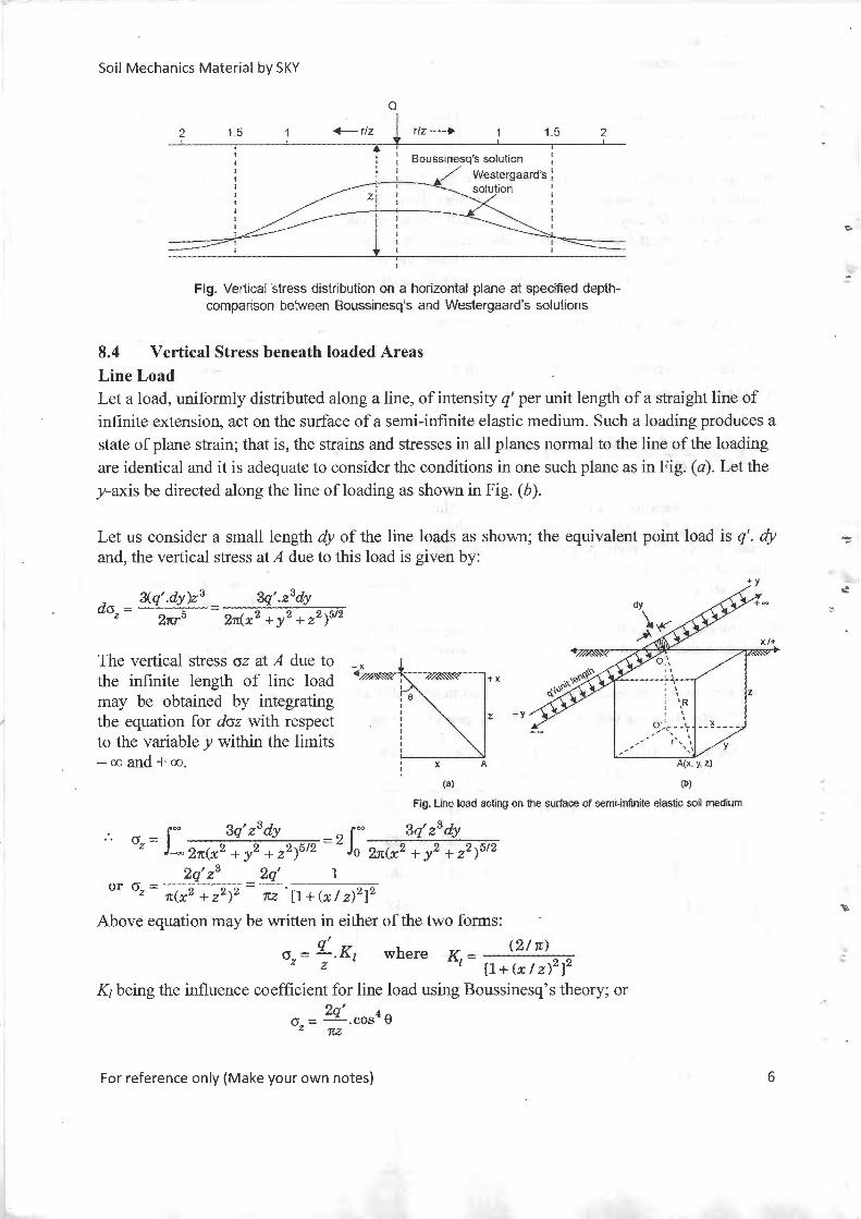
Fig. Vertical stress distribution on a horizontal plane at specified depthcomparison between Boussinesq's and Westergaard's solutions

8.4 Vertical Stress beneath loaded Areas Line Load Let a load, uniformly distributed along a line, of intensity q' per unit length of a straight line of infinite extension, act on the surface of a semi-infinite elastic medium. Such a loading produces a state of plane strain; that is, the strains and stresses in all planes normal to the line of the loading are identical and it is adequate to consider the conditions in one such plane as in Fig. (a). Let the y-axis be directed along the line ofloading as shown in Fig. (b) .

'Co

:,

Let us consider a small length dy of the line loads as shown; the equivalent point load is q'. dy ~ and, the vertical stress at A due to this load is given by:

3(q' .dy )z3 3q' .z3dy d02 = 2n:r5 = 2n:(x2 + y2 + z2 )5/2

The vertical stress crz at A due to the infinite length of line load may be obtained by integrating the equation for dcrz with respect to the variable y within the limits - oo and+ oo.

-x _.:;v~~rs· ·····;zr~VT····· I+ x

e z

x A

(a)

-y O,' _\_t __ L __ _ .;,- \

,,.., ~ ... , \ A ,/ ~

A(x, y, Z)

(b)

Fig. Line load acting on the surface of semi-infinite elastic soil medium

Joo 3q' 2 3dy r= 3q' 2 3dy

. . crz = -= 2n(x2 + y2 + 22 )5/2 = 2 Jo 2n(x2 + y2 + 22 )5/2

2q' 2 3 2q' 1 or cr~ = 9 9; = - . -···········-······· ·;;>

"' n(x~ + 2~)2 nz [l + (x I 2) 2 ]~

Above equation may be written in either of the two forms : q' (2/n)

cr = - .K 1 where K = ----z z 1 [l + (x I z )2 ]2

K1 being the influence coefficient for line load using Boussinesq' s theory; or 2q' 4

0 =-.cos e z nz


" .:

z

""

~·

-.:.."

6

..

'\

"'

'\

.:


Ux and Txz may be also derived and shown to be: 2 q' 2 . 2

cr = . cos 8. sm 8 x 7t z

2 q' 2 . 1 = -.-.cos 8.sme

xz 1t z

If the point A is situated vertically below the line load, at a depth z, we have x = 0, and hence the vertical stress is then given by:

STRIP LOAD

2 q' <Jz = n Z

A strip load is the load transmitted by a structure of finite width and infinite length on a soil surface. Two types of strip loads are common in geotechnical engineering. One is a load that imposes a uniform stress on the soil, for example, the middle section of a long embankment (Figure a). The other is a load that induces a triangular stress distribution over an area of width B (Figure b ). An example of a strip load with a triangular stress distribution is the stress under the side of an embankment. The increases in stresses due to a surface stress qs (force/area) are as follows:

(a) Area transmitting a uniform stress (Figure a)

6.a" = qs [a + sin a cos( a+ 2~)] - 'IT

Llux = qs[a - sinacos(cx + 2(3)] 'IT

LlTzx = q~ [sin a sin( a+ 2~)] 'IT

where q5 is the applied surface stress.

(b) Area transmitting a triangular stress (Figure b)

Qs(X 1 . ) Au, = - -a - -sm 2(j ~ 7r B 2

qs (x z Ri 1 . ) Aa = - -ex - -In-+ -sm2R. x 7r B B R~ 2 1.1

Qs ( Z ) AT zx = 2

1T 1 + cos 2f3 - 2 B a

where q5 is the applied surface stress.


x

(b)

~

~

7


(c) Area transmitting a uniform stress near a retaining wall (Figure c, d)

f-<--B--+I a ---/--- B~ ii I I I I I I ii

qs(force/area) ii I I I I I I ii

i'

•·-r- l T '

zl _rl-zi f

Ho Ho

1 (c) 1 (d)

2qy LlaK = -(13 - sin f3 cos 2a)

. 'lT

The lateral force and its location were derived by Jarquio (1981) and are

qs . LlPx =

90[H0 (02 - 01 )]

z = H~(02 - 01) - (R1 - R1) + 57.3BHo

2H0 (02 - 01)

where ( ) ( + B) 01 = tan- 1 ;

0

, 02 = tan- 1 a Ho

R 1 = (a + B)2 (90 - 02 ), and R2 = a2 (90 - 81)

Uniformly Loaded Circular Area The Boussinesq equation for the vertical stress due to a point load can be extended to find the vertical stress at any point beneath the centre of a uniformly loaded circular area. Let the circular area of radius a be loaded uniformly with q per unit area as shown in Figure.

Let us consider an elementary ring of radius r and thickness dr of the loaded area. This ring may be imagined to be further divided into elemental areas, each oA ; the load from such an elemental area is q . oA . The vertical stress o 0 2 at point A, at a depth z below the centre of the loaded area, is given by:

qs(force/area)

ocr = 3(q.M). z3

z 27t (r2 + z2 )5/2 Fig. Uniform load over circular area


~

"::..

::.

8

'· J

.. ...

_j

Soil Mechanics Mate rial by SKY

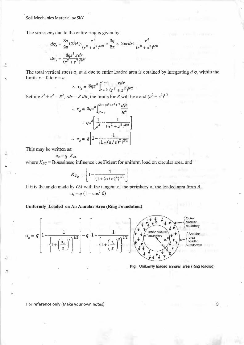
The stress da::: due to the entire ring is given by:

3q . z 3 3q z 3

da - - (LbA) ----- = --- x (2rcrdr) --- -z - 2n · (r2 + z 2 )5/2 2n · (r2 + z 2 )5/ 2

3qz3.rdr da = 9 2 •

z (r- + z )o

The total vertical stress cr2 at A due to entire loaded area is obtained by integrating d a2 within the limits r = 0 to r = a.

3fr =a rdr . - 3 z • • (Jz - q ( 2 2 )5/2 r=O r +z

Setting r2 + z2 = R2, rdr = R.dR, the limits for R will be z and (a2 + z2) 112

.

3 R = (a2+z2>112 dR .. cr = 3qz J -

z R=z R4

3[ 1 1 l = qz -- ? z3 (a2+z-)312

.. cr,= q[l - {l+(a~z>'l'" l This may be written as:

Ciz = q. Ksc where K8c = Boussinesq influence coefficient for uniform load on circular area, and

KB -[1-- --1--] c - {l+(a/z)2}3/2

If 8 is the angle made by OA with the tangent of the periphery of the loaded area from A,

0 2 = q (1 - cos3 8)

Uniformly Loaded on An Annular Area (Ring Foundation)

(Jz = q 1-

{i+( ~ rr 1 -q 1-

{i+( :; rr 1


{

Outer circular boundary

{

Annular area loaded uniformly

·Fig. Uniformly loaded annular area (Ring loading)

9

Soil Mechanics Materia l by SKY

Uniformly Loaded Rectangular Area

Newmark (1935) has derived an expression for the vertical stress at a point below the corner of a rectangular area loaded uniformly as shown in Figure.

The following is the popular form of

Newmark' s equation for crz: which is

widely used for the calculation purpose. 1~ z

11

/ /

/

/ /

/

B ...i.

~ ~

CTz = qlcr Fig. Vertical stress at the corner of a uniformly loaded rectangu lar area

q (2mnm +n +1) (m +n +2) _1 2mnm +n +1

[

J2 2 2 2 J2 2 J <Jz= 4n (m 2 +n 2 +1+m 2n 2 ).(m2 +n 2 +1) +tan (m 2 +n 2 +1-m2n 2

where m =Biz and n =Liz, as explained in the figure above and the second term within the

brackets is an angle in radians. The above equation may be written in the form: cr2 = q. Ia

where Ia= Influence value

)[[. 2mnJm

2 + n

2 + 1 J (m 2

+ n 2

+ 2J _1 [ . 2mnJm 2

+ n 2

+ 1 J. J I = (1/ 4 rr <> 2 2 2 · •) <> +tan 2 2 2 2

cr m~ +n +l+m n m- +n~ +1 m +n +l-m n

You can program your calculator or use a spreadsheet program to find Ia . You must be careful in the last term (tan-1

) in programming. If m2 + n2 + 1 < m2n2, then you have to add n to the

bracketed quantity in the last term.

In most cases the vertical stress increase below the center of a rectangular area is important. This stress increase can be given by the relationship

where O"z = qi

2 [ m 1n 1 1 + mf + 2nf

I = 1T vi.+ ~~T -+ nf (1 + nf)(mf + nf) . - 1 1111 ]

+ sm -v;;;f +··;;i vi ·+-· nr L z B

111 1 = - , n 1 = - ; b = -B b 2


~

~ ..

!!·

. '

~

.!.

/.

... """

~

~

.....

'-'

'

~

Soil Mee

-"

v

,,,r=:? t ,..- <" B---,~-/ x ~

1illcrz A = 1 q u(f_ • s

m and n ;re i~terchangeable

m = Bn=L 7' ""' ~ ,.,

Value of n

0.01 2 3 4 5 6 80.l 2 3

Value of n 6 81 .0 2 3456810

28 I 1111 I I I I 11111.28

Tm:;:3.o .26 I I I I I ~n=2 . 5 .26

m=2.0 '-"+-'k~'""1"""1 - r ~m=l.8'---.,_,

11 I~ .24 .24 f-hn=l.6~ I I

22 lllnfm~n ~1+-Jh£-~~-l--l-_L-Ll.-Ll--l.18

.16 .16

.14 .14

.12 .12

u) .10 .10 ~ m=0.3 g; (1) gre re (1) ::l

;:;::: c m=0.2 - .061----t- l-W--W---if!llll..~r....+,.i!'.-1-1--l-l--=-~=t:=:t=l=+:!=l:::t:l.C6

.04 I I I I H .04 m=O.l

D2 -~

O m=O.O O 0.01 0.1 1.0 10

Value of n

FIGURE Influence factor for calculating the vertical stress increase under the corner of a rectangle.

(Source: NAV-FAC-DM 7.1.)

8.5 New marks influence Chart It may not be possible to use Fadum's influence coefficients or chart for irregularly shaped loaded areas. Newmark (1942) devised a simple, graphical procedure for computing the vertical stress in the interior of a soil medium, loaded by uniformly distributed, vertical load at the surface. The chart devised by him for this purpose is called an ' Influence Chart' . This is applicable to a semi-infinite, homogeneous, isotropic and elastic soil mass (and not for a stratified soil).



The operation or use of the Newmark's chart is as follows:

The chart can be used for any uniformly loaded area of whatever shape that may be.

First, the loaded area is drawn on a tracing paper, using the same scale to which the distance ON on the chart represents the specified depth; the point at which the vertical stress is desired is then placed over the centre of the circles on the chart.

For example: The diagram can be used for any other values of the depth z by simply assuming that the scale to which it is drawn alters; thus, if z is to be 5 m the line ON now represents 5 m and the scale is therefore 1 cm = 1 m (similarly, if z = 20 m, the scale becomes 1cm=4 m). Fig. Newmark's influence chart

The number of influence units encompassed by or contained in the boundaries of the loaded area are counted, including fractional units, if any; let this total equivalent number be N.

The stress cr2 at the specified depth at the specified point is then given by: cr2 = I. N q, where I= influence value of the chart.

(Note: The stress may be found at any point which lies either inside or outside the loaded area with the aid of the chart).

Although it appears remarkably simple, Newmark's chart has also some inherent deficiencies:

1. Many loaded areas have to be drawn; alternatively, many influence charts have to be drawn. 2. For each different depth, counting of the influence meshes must be done. Considerable amount

of guesswork may be required in estimating the influence units partially covered by the loaded area.

However, the primary advantage is that it can be used for loaded area of any shape and that it is relatively rapid. This makes it attractive.


- --- 1

.... ""'

.. -

"e

... "

.:

... ~

~

~-

~·

~

'I.


8.6 Approximate stress distribution method for loaded Areas.

Equivalent Point Load Method

In this approach, the given loaded area is divided into a convenient number of smaller units and the total load from each unit is assumed to act at its centroid as a point load.

The principle of superposition is then applied and the required stress at a specified point is obtained by summing up the contributions of the individual point loads from each of the units by applying the appropriate Point Load formula, such as that of Boussinesq.

Referring to Fig, if the influence values are K8 1,

K82,. .. for the point loads Q1,Q2, .. ., for az at A, we have:

CTz = (Q1Ks1 + QzKs2 + ... )

Two is to One Method

This method involves the assumption that the stresses get distributed uniformly on to areas the edges of which are obtained by taking the angle of distribution at 2 vertical to 1 horizontal (tan 8 = 112), where 8 is the angle made by the line of distribution with the vertical, as shown in Figure.

The average vertical stress at depth z is obtained as:

q.B.L (j -----

Zal' - (B + Z )(£ + Z)

2

l-4

I I I

B ' .. 1 ' ' ' ' ' ' ' ' '

\ \

I \

I I I

\ \ I \ \ I

' ' R '

z

' \ \ 2 \ ' R '' R ' 4\\ I 3 ' \ \ \ R1 ', ,, '

' \\ I ' ,, \

'' ,'\.\ ',\,,A

crz Fig. Equivalent point load method

B

2

Fig. Two is to one method

The average vertical stress cr2 depends upon the shape of the loaded area, given as below:

I.Square Area (Bx B). 2. Circular Area (diameter D) 3. Strip Area (width B, unit length) qB2

<Jz = (B+Z) 2

qD2

(Jz = (D+Z) 2


q(Bxl) (Jz = (BxZ)xl

13

Soil Mechanics Material by SKY -...

Documents

Transcript of Soil Mechanics Material by SKY -...