A Fourier pseudospectral method for the good Boussinesq ...

A Fourier Pseudospectral Method for the “Good”Boussinesq Equation with Second-OrderTemporal AccuracyKelong Cheng,1 Wenqiang Feng,2 Sigal Gottlieb,3 Cheng Wang3

1Department of Mathematics, Southwest University of Science and Technology,Mianyang, Sichuan 621010, People’s Republic of China

2Department of Mathematics, University of Tennessee, Knoxville, Tennessee 379963Department of Mathematics, University of Massachusetts, North Dartmouth,Massachusetts 02747

Received 24 January 2014; accepted 22 May 2014Published online 24 June 2014 in Wiley Online Library (wileyonlinelibrary.com).DOI 10.1002/num.21899

In this article, we discuss the nonlinear stability and convergence of a fully discrete Fourier pseudospectralmethod coupled with a specially designed second-order time-stepping for the numerical solution of the“good” Boussinesq equation. Our analysis improves the existing results presented in earlier literature intwo ways. First, a �∞(0, T ∗; H 2) convergence for the solution and �∞(0, T ∗; �2) convergence for the time-derivative of the solution are obtained in this article, instead of the �∞(0, T ∗; �2) convergence for the solutionand the �∞(0, T ∗; H−2) convergence for the time-derivative, given in De Frutos, et al., Math Comput 57(1991), 109–122. In addition, we prove that this method is unconditionally stable and convergent for thetime step in terms of the spatial grid size, compared with a severe restriction time step restriction �t ≤ Ch2

required by the proof in De Frutos, et al., Math Comput 57 (1991), 109–122. © 2014 Wiley Periodicals, Inc.Numer Methods Partial Differential Eq 31: 202–224, 2015

Keywords: aliasing error; fully discrete Fourier pseudospectral method; good Boussinesq equation; stabilityand convergence

I. INTRODUCTION

The soliton-producing nonlinear wave equation is a topic of significant scientific interest. Onecommonly used example is the so-called “good” Boussinesq (GB) equation

utt = −uxxxx + uxx + (up)xx , with an integer p ≥ 2. (1.1)

Correspondence to: Cheng Wang, Department of Mathematics, University of Massachusetts, 285 Old Westport Road,North Dartmouth, MA 02747 (e-mail: [email protected])Contract grant sponsor: Air Force Office of Scientific Research (to S. G); contract grant number: FA-9550-12-1-0224Contract grant sponsor: NSF (to C. W); contract grant number: DMS-1115420Contract grant sponsor: NSFC (to C. W.); contract grant number: 11271281

© 2014 Wiley Periodicals, Inc.

A FOURIER PSEUDOSPECTRAL METHOD 203

It is similar to the well-known Korteweg-de Vries (KdV) equation; a balance between disper-sion and nonlinearity leads to the existence of solitons. The GB equation and its various extensionshave been investigated by many authors. For instance, a closed form solution for the two solitoninteraction of Eq. (1.1) was obtained by Manoranjan et al. in [1] and a few numerical experimentswere performed based on the Petrov–Galerkin method with linear “hat” functions. In [2], it wasshown that the GB equation possesses a highly complicated mechanism for the solitary wavesinteraction. Ortega and Sanz-Serna [3] discussed nonlinear stability and convergence of somesimple finite difference schemes for the numerical solution of this equation. More analytical andnumerical works related to GB equations can be found in the literature, for example, [4–15].

In this article, we consider the GB equation (1.1), with a periodic boundary condition over anone-dimensional (1D) domain � = (0,L) and initial data u(x, 0) = u0(x), ut(x, 0) = v0(x), bothof which are L-periodic. It is assumed that a unique, periodic, smooth enough solution exists for(1.1) over the time interval (0,T ). This L-periodicity assumption is reasonable if the solution to(1.1) decays exponentially outside [0,L].

Due to the periodic boundary condition, the Fourier collocation (pseudospectral) differentia-tion is a natural choice to obtain the optimal spatial accuracy. There has been a wide and variedliterature on the development of spectral and pseudospectral schemes. For instance, the stabilityanalysis for linear time-dependent problems can be found in [16, 17], and so forth, based oneigenvalue estimates. Some pioneering works for nonlinear equations were initiated by Madayand Quarteroni [18–20] for steady-state spectral solutions. Also, note the analysis of 1D con-servation laws by Tadmor and coworkers [21–27], semidiscrete viscous Burgers’ equation andNavier–Stokes equations by Weinan [28, 29], the Galerkin spectral method for Navier–Stokesequations led by Guo [22, 30–32] and Shen [33, 34], and the fully discrete (discrete both in spaceand time) pseudospectral method applied to viscous Burgers’ equation in [11] by Gottlieb andWang and [35] by Bressan and Quarteroni, and so forth.

In addition, an application of spectral and pseudospectral approximation to dispersive nonlin-ear wave equation, such as KdV equation has attracted a great deal of attention. Many interestingtheoretical analysis and numerical results have been reported in the existing literature; for exam-ple, see [36] for the semidiscrete spectral methods, [37] for the error estimate of a fully discretescheme, and [38, 39] for the error estimates of the Benjamin–Ono equation or related nonlocalmodels, and so forth. For the GB equation (1.1), it is worth mentioning De Frutos et al.’s work[10] on the nonlinear analysis of a second-order (in time) pseudospectral scheme for the GBequation (with p = 2). However, as the authors point out in their remark on page 119, thesetheoretical results were not optimal: “... our energy norm is an L2-norm of u combined with anegative norm of ut . This should be compared with the energy norm in [40]: there, no integra-tion with respect to x is necessary and convergence is proved in H2 for u and L2 for ut .” Thedifficulties in the analysis are due to the absence of a dissipation mechanism in the GB equation(1.1), which makes the nonlinear error terms much more challenging to analyze than that of aparabolic equation. The presence of a second-order spatial derivative for the nonlinear term leadsto an essential difficulty of numerical error estimate in a higher order Sobolev norm. In additionto the lack of optimal numerical error estimate, the analysis in [10] also imposes a severe timestep restriction: �t ≤ Ch2 (with C a fixed constant), in the nonlinear stability analysis. Such aconstraint becomes very restrictive for a fine numerical mesh and leads to a high computationalcost.

In this work, we propose a second-order (in time) pseudospectral scheme for the GB equa-tion (1.1) with an alternate approach, and provide a novel nonlinear analysis. In more detail, a�∞(0, T ∗; H 2) convergence for u and �∞(0, T ∗; �2) convergence for ut are derived, compared withthe �∞(0, T ∗; �2) convergence for u and �∞(0, T ∗; H−2) convergence for ut , as reported in [10].

Numerical Methods for Partial Differential Equations DOI 10.1002/num

204 CHENG ET AL.

Furthermore, such a convergence is unconditional (for the time step �t in terms of space gridsize h) so that the severe time step constraint �t ≤ Ch2 is avoided.

The methodology of the proposed second-order temporal discretization is very different fromthat in [10]. To overcome the difficulty associated with the second-order temporal derivative in thehyperbolic equation, we introduce a new variable ψ to approximate ut , which greatly facilitatesthe numerical implementation. Conversely, the corresponding second-order consistency analysisbecomes nontrivial because of a O(�t2) numerical error between the centered difference of uand the midpoint average of ψ . Without a careful treatment, such a O(�t2) numerical error mightseem to introduce a reduction of temporal accuracy, because of the second-order time deriva-tive involved in the equation. To overcome this difficulty, we perform a higher order consistencyanalysis by an asymptotic expansion; as a result, the constructed approximate solution satisfiesthe numerical scheme with a higher order truncation error. Furthermore, a projection of the exactsolution onto the Fourier space leads to an optimal regularity requirement.

For the nonlinear stability and convergence analysis, we have to obtain a direct estimate of the(discrete) H2 norm of the nonlinear numerical error function. This estimate relies on the aliasingerror control lemma for pseudospectral approximation to nonlinear terms, which was proven in arecent work [11]. That is the key reason we are able to overcome the key difficulty in the nonlinearestimate and obtain a �∞(0, T ∗; H 2) convergence for u and �∞(0, T ∗; �2) convergence for ut . Weprove that the proposed numerical scheme is fully consistent (with a higher order expansion),stable and convergent in the H2 norm up to some fixed final time T ∗. In turn, the maximum normbound of the numerical solution is automatically obtained, because of the H2 error estimate andthe corresponding Sobolev embedding. Therefore, the inverse inequality in the stability analysisis not needed and any scaling law between �t and h is avoided, compared with the �t ≤ Ch2

constraint reported in [10].This article is outlined as follows. In Section II, we review the Fourier spectral and pseu-

dospectral differentiation, recall an aliasing error control lemma (proven in [11]), and presentan alternate second-order (in time) pseudospectral scheme for the GB equation (1.1). In SectionIII, the consistency analysis of the scheme is studied in detail. The stability and convergenceanalysis is reported in Section IV. A simple numerical result is presented in Section V. Finally,some concluding remarks are made in Section VI.

II. THE NUMERICAL SCHEME AND THE MAIN RESULT

A. Review of Fourier Spectral and Pseudospectral Approximations

For f (x) ∈ L2(�), � = (0, L), with Fourier series

f (x) =∞∑

l=−∞fle

2π ilx/L, with fl =∫

�

f (x)e−2π ilx/Ldx, (2.1)

its truncated series is defined as the projection onto the space BN of trigonometric polynomialsin x of degree up to N, given by

PNf (x) =N∑

l=−N

fle2π ilx/L. (2.2)



To obtain a pseudospectral approximation at a given set of points, an interpolation operator IN

is introduced. Given a uniform numerical grid with (2N + 1) points and a discrete vector function fwhere fi = f (xi), for each spatial point xi . The Fourier interpolation of the function is defined by

(INf )(x) =N∑

l=−N

(f Nc )

le2π ilx/L, (2.3)

where the (2N + 1) pseudospectral coefficients (f Nc )

lare computed based on the interpolation con-

dition f (xi) = (INf )(xi) on the 2N + 1 equidistant points [41–43]. These collocation coefficientscan be efficiently computed using the fast Fourier transform (FFT). Note that the pseudospectralcoefficients are not equal to the actual Fourier coefficients; the difference between them is knownas the aliasing error. In general, PNf (x) �= INf (x), and even PNf (xi) �= INf (xi), except ofcourse in the case that f ∈ BN .

The Fourier series and the formulas for its projection and interpolation allow one to easily takederivative by simply multiplying the appropriate Fourier coefficients (f N

c )l

by 2lπ i/L. Further-more, we can take subsequent derivatives in the same way, so that differentiation in physical spaceis accomplished via multiplication in Fourier space. As long as f and all is derivatives (up to mthorder) are continuous and periodic on �, the convergence of the derivatives of the projection andinterpolation is given by

||∂kf (x) − ∂kPNf (x)|| ≤ C||f (m)||hm−k , for 0 ≤ k ≤ m,

||∂kf (x) − ∂kINf (x)|| ≤ C||f ||Hmhm−k , for 0 ≤ k ≤ m, m >d

2, (2.4)

in which ||·|| denotes the L2 norm. For more details, see the discussion of approximation theoryby Canuto and Quarteroni [44].

For any collocation approximation to the function f (x) at the points xi

f (xi) = (INf )i =N∑

l=−N

(f Nc )

le2π ilxi , (2.5)

one can define discrete differentiation operator DN operating on the vector of grid valuesf = f (xi). In practice, one may compute the collocation coefficients (f N

c )l

via FFT, and thenmultiply them by the correct values (given by 2lπ i) and perform the inverse FFT. Alternatively,we can view the differentiation operator DN as a matrix, and the above process can be seen asa matrix-vector multiplication. The same process is performed for the second and fourth deriv-atives ∂2

x , ∂4x , where this time the collocation coefficients are multiplied by (−4π 2l2/L2) and

(16π 4l4/L4), respectively. In turn, the differentiation matrix can be applied for multiple times,that is, the vector f is multiplied by D2

N and D4N , respectively.

Because the pseudospectral differentiation is taken at a point-wise level, a discrete L2 norm andinner product need to be introduced to facilitate the analysis. Given any periodic grid functions fand g (over the numerical grid), we note that these are simply vectors and define the discrete L2

inner product and norm

‖f‖2 = √〈f , f〉, with 〈f , g〉 = 1

2N + 1

2N∑i=0

figi . (2.6)


206 CHENG ET AL.

The following summation by parts (see [11]) will be of use:

〈f , DNg〉 = −〈DN f , g〉, 〈f , D2Ng〉 = −〈DN f , DNg〉, 〈f , D4

Ng〉 = 〈D2N f , D2

Ng〉. (2.7)

B. An Aliasing Error Control Estimate in Fourier Pseudospectral Approximation

This lemma, established in [11], allows us to bound the aliasing error for the nonlinear term, andwill be critical to our analysis. For any function ϕ(x) in the space BpN , its collocation coeffi-cients qN

l are computed based on the 2N + 1 equidistant points. In turn, INϕ(x) is given by thecontinuous expansion based on these coefficients:

INϕ(x) =N∑

l=−N

qNl e2π ilx/L. (2.8)

Since ϕ(x) ∈ BpN , we have INϕ(x) �= PNϕ(x) due to the aliasing error.The following lemma enables us to obtain an Hm bound of the interpolation of the nonlinear

term; the detailed proof can be found in [11].

Lemma 2.1. For any ϕ ∈ BpN (with p an integer) in dimension d, we have

‖INϕ‖Hk ≤ (√

p)d‖ϕ‖Hk . (2.9)

C. Formulation of the Numerical Scheme and the Convergence Result

We propose the following fully discrete second-order (in time) scheme for Eq. (1.1):⎧⎪⎪⎪⎨⎪⎪⎪⎩

ψn+1 − ψn

�t= − D4

N

(un+1 + un

2

)+ D2

N

(un+1 + un

2

)+ D2

N

(3

2(un)

p − 1

2(un−1)

p

),

un+1 − un

�t= ψn+1 + ψn

2,

(2.10)

whereψ is a second-order approximation to ut and DN denotes the discrete differentiation operator.The main result of this article is given later.

Theorem 2.2. For any final time T > 0, assume the exact solution ue to the GB equation (1.1)given by (3.21). Denote u�t ,h as the continuous (in space) extension of the fully discrete numericalsolution given by scheme (2.10). As �t , h → 0, the following convergence result is valid:

‖u�t ,h − ue‖�∞(0,T ∗;H2) + ‖ψ�t ,h − ψe‖�∞(0,T ∗;L2) ≤ C(�t2 + hm), (2.11)

provided that the time step �t and the space grid size h are bounded by given constants which areonly dependent on the exact solution. Note that the convergence constant in (2.11) also dependson the exact solution as well as T.

Remark 2.3. With a substitution ψn+1 = 2(un+1−un)

�t−ψn, the scheme (2.10) can be reformulated

as a closed equation for un+1:

2un+1

�t2+ 1

2(D4

N − D2N)un+1 = D2

N

(3

2(un)

p − 1

2(un−1)

p

)− 1

2(D4

N − D2N)un +

2un

�t+ 2ψn

�t.

(2.12)



As the treatment of the nonlinear term is fully explicit, this resulting implicit scheme requiresonly a linear solver. Furthermore, a detailed calculation shows that all the eigenvalues of thelinear operator on the left-hand side are positive, and so the unique unconditional solvability ofthe proposed scheme (2.10) is assured. In practice, the FFT can be used to efficiently obtain thenumerical solutions.

Remark 2.4. An introduction of the variable ψ allows us to rewrite the wave equation as afirst-order system in time. This rewritten form not only facilitates the numerical implementation,but also improves the numerical stability. The stability analysis and error estimate for the linearversion of (2.10) were provided in an earlier article [45].

Remark 2.5. In contrast, three time steps tn+1, tn, and tn−1 are involved in the numericalapproximation to the second-order temporal derivative as presented in the earlier work [10] (withp = 2):

un+1 − 2un + un−1

�t2= −1

4D4

N(un+1 + 2un + un−1) + D2Nun + D2

N((un)2). (2.13)

A careful analysis in [10] shows that the numerical stability for (2.13) could only be theoreti-cally justified under a severe time step constraint �t ≤ Ch2, although an intuitive and linearizedstability analysis, as well as the numerical results, indicate that a standard Courant–Friedrichs–Lewy (CFL) condition �t = O(h) is sufficient. Conversely, the special structure of our proposedscheme (2.10) results in an unconditional stability and convergence for a fixed final time, as willbe presented in later analysis.

These subtle differences in terms of the stability conditions will be analyzed in later sections.See Remarks 4.3–4.6 below.

III. THE CONSISTENCY ANALYSIS

In this section, we establish a truncation error estimate for the fully discrete scheme (2.10) for theGB equation (1.1). A finite Fourier projection is applied to the exact solution of the GB equation(1.1) and a local truncation error is derived. Moreover, we perform a higher order consistencyanalysis in time, through an addition of a correction term, so that the constructed approximatesolution satisfies the numerical scheme with higher order temporal accuracy. This approach avoidsa key difficulty associated with the accuracy reduction in time due to the appearance of the secondin time temporal derivative.

A. Truncation Error Analysis for UN

Given the domain � = (0,L), the uniform mesh grid (xi), 0 ≤ i ≤ 2N , and the exact solution ue,we denote UN as its projection into BN :

UN(x, t) := PNue(x, t). (3.1)

The following approximation estimates are clear:

‖UN − ue‖L∞(0,T ∗;Hr ) ≤ Chm‖ue‖L∞(0,T ∗;Hm+r ), for r ≥ 0, (3.2)

‖∂kt (UN − ue)‖Hr ≤ Chm‖∂k

t ue‖Hm+r , for r ≥ 0, 0 ≤ k ≤ 4, (3.3)


208 CHENG ET AL.

in which the second inequality comes from the fact that ∂kt UN is the truncation of ∂k

t ue for anyk ≥ 0, as projection and differentiation commute:

∂k

∂tkUN(x, t) = ∂k

∂tkPNue(x, t) = PN

∂kue(x, t)

∂tk. (3.4)

As a direct consequence, the following linear estimates are straightforward:

‖∂2t (UN − ue)‖L2 ≤ Chm‖∂2

t ue‖Hm , (3.5)

‖∂2x (UN − ue)‖L2 ≤ Chm‖ue‖Hm+2 , ‖∂4

x (UN − ue)‖L2 ≤ Chm‖ue‖Hm+4 . (3.6)

Conversely, a discrete ‖ · ‖2 estimate for these terms is needed in the local truncation derivation.To overcome this difficulty, we observe that

‖∂2t (UN − ue)‖2 = ‖IN(∂2

t (UN − ue))‖L2 ≤ ‖∂2t (UN − ue)‖L2 + ‖∂2

t (INue − ue)‖L2 , (3.7)

in which the second step comes from the fact that IN∂2t UN = ∂2

t UN , since ∂2t UN ∈ BN . The first

term has an estimate given by (3.5), whereas the second term could be bounded by

‖(∂2t (INue − ue))‖L2 = ‖IN(∂2

t ue) − ∂2t ue‖L2 ≤ Chm‖∂2

t ue‖Hm , (3.8)

as an application of (2.4). In turn, its combination with (3.7) and (3.5) yields

‖∂2t (UN − ue)‖2 ≤ Chm‖∂2

t ue‖Hm . (3.9)

Using similar arguments, we also arrive at

‖∂2x (UN − ue)‖2 ≤ Chm‖ue‖Hm+2 , ‖∂4

x (UN − ue)‖2 ≤ Chm‖ue‖Hm+4 . (3.10)

For the nonlinear term, we begin with the following expansion:

∂2x (u

pe ) = p((p − 1)up−2

e (ue)2x + up−1

e (ue)xx), which in turn gives

∂2x (u

pe − (UN)p) = p

((p − 1)U

p−2N (ue + UN)x(ue − UN)x

+ (p − 1)(ue − UN)(ue)2x

p−3∑k=0

ukeU

p−3−k

N

+ Up−1N (ue − UN)xx + (ue − UN)(ue)xx

p−2∑k=0

ukeU

p−2−k

N

). (3.11)

Subsequently, its combination with (3.2) implies that

‖∂2x (u

pe − (UN)p)‖

L2

≤ C(‖UN‖p−2L∞ · ‖ue + UN‖W1,∞ · ‖ue − UN‖H1 + ‖UN‖p−1

L∞ · ‖ue − UN‖H2

+ ‖ue − UN‖L∞ · (‖ue‖p−2L∞ + ‖UN‖p−2

L∞ ) · (‖ue‖H2 + ‖ue‖2W1,4))

≤ C(‖UN‖p−2

H1 · ‖ue + UN‖H2 · ‖ue − UN‖H1 + ‖UN‖p−1

H1 · ‖ue − UN‖H2

+ ‖ue − UN‖H1 · (‖ue‖p−2

H1 + ‖UN‖p−2

H1 ) · (‖ue‖H2 + ‖ue‖2H2))



≤ C(‖ue‖p

H2 + ‖UN‖p

H2) · ‖ue − UN‖H2

≤ C‖ue‖p

H2 · ‖ue − UN‖H2 ≤ Chm‖ue‖p

H2 · ‖ue‖Hm+2 , (3.12)

in which an 1D Sobolev embedding was used in the second step.The following interpolation error estimates can be derived in a similar way, based on (2.4):

‖∂2x (u

pe ) − IN(∂2

x (upe ))‖L2 ≤ Chm‖∂2

x (upe )‖Hm ≤ Chm‖ue‖p

H2 · ‖ue‖Hm+2 , (3.13)

‖∂2x (U

p

N) − IN(∂2x (U

p

N))‖L2 ≤ Chm‖∂2

x (Up

N)‖Hm ≤ Chm‖ue‖p

H2 · ‖ue‖Hm+2 . (3.14)

In turn, a combination of (3.12)–(3.14) implies the following estimate for the nonlinear term

‖∂2x (u

pe − (UN)p)‖2 = ‖IN(∂2

x (upe − (UN)p))‖

L2

≤ ‖∂2x (u

pe − (UN)p)‖

L2 + ‖∂2x (u

pe ) − IN(∂2

x (upe ))‖L2

+ ‖∂2x (U

p

N) − IN(∂2x (U

p

N))‖L2 ≤ Chm‖ue‖p

H2 · ‖ue‖Hm+2 . (3.15)

By observing (3.9), (3.10), and (3.15), we conclude that UN satisfies the original GB equation(1.1) up to a O(hm) (spectrally accurate) truncation error:

∂2t UN = −∂4

xUN + ∂2xUN + ∂2

x (Up

N) + τ0, with ‖τ0‖2 ≤ Chm(‖ue‖p

H2 + 1) · ‖ue‖Hm+4 .(3.16)

Moreover, we define the following profile, a second-order (in time) approximation to ∂tue:

N(x, t) := ∂tUN(x, t) − �t2

12∂3

t UN(x, t). (3.17)

For any function G = G(x,t), given n > 0, we define Gn(x) := G(x, n�t).

B. Truncation Error Analysis in Time

For simplicity of presentation, we assume T = K�t with an integer K. The following two pre-liminary estimates are excerpted from a recent work [46], which will be useful in later consistencyanalysis.

Proposition 3.1 ([46]). For f ∈ H 3(0, T ), we have

‖τ tf ‖�2(0,T ) ≤ C�tm‖f ‖Hm+1(0,T ), with τ tf n = f n+1 − f n

�t− f ′(tn+1/2), (3.18)

for 0 ≤ m ≤ 2, where C only depends on T , ‖ · ‖�2(0,T ) is a discrete L2 norm (in time) given by

‖g‖�2(0,T ) =√

�t∑K−1

n=0 (gn)2.

Proposition 3.2 ([46]). For f ∈ H 2(0, T ), we have

‖D2t/2f ‖

�2(0,T ):=

(�t

K−1∑n=0

(D2

t/2fn+1/2

)2

) 12

≤ C‖f ‖H2(0,T ), (3.19)


210 CHENG ET AL.

‖D2t f ‖

�2(0,T ):=

(�t

K−1∑n=0

(D2

t fn)2

) 12

≤ C‖f ‖H2(0,T ),

with D2t/2f

n+1/2 = 4(f n+1 − 2f ( · , tn+1/2) + f n)

�t2, D2

t fn = f n+1 − 2f n + f n−1

�t2, (3.20)

where C only depends on T.

The following theorem is the desired consistency result. To simplify the presentation below,for the constructed solution (UN , ψN), we define its vector grid function (Un, n) = I(UN , ψN)

as its interpolation: Uni = Un

N(xi , tn), ni = n

N(xi , tn).

Theorem 3.1. Suppose the unique periodic solution for Eq. (1.1) satisfies the followingregularity assumption

ue ∈ H 4(0, T ; L2) ∩ L∞(0, T ; Hm+4) ∩ H 2(0, T ; H 4). (3.21)

Set (UN , N) as the approximation solution constructed by (3.1), (3.17) and let (U , ) as itsdiscrete interpolation. Then, we have⎧⎪⎪⎪⎨⎪⎪⎪⎩

n+1 − n

�t= −D4

N

(Un+1 + Un

2

)+ D2

N

(Un+1 + Un

2

)+ D2

N

(3

2(Un)

p − 1

2(Un−1)

p

)+ τ n

1 ,

Un+1 − Un

�t= n+1 + n

2+ �tτn

2 ,

(3.22)

where τ ki satisfies

‖τi‖�2(0,T ;�2) :=(

�t

K∑k=0

‖τ ki ‖2

2

) 12

≤ M(�t2 + hm), i = 1, 2, (3.23)

in which M only depends on the regularity of the exact solution ue.

Proof. We define the following notation:

Fn+1/20 = Un+1−Un

�t,

Fn+1/21 = n+1−n

�t, F

n+1/21e = (∂2

t UN)(·, tn+1/2),

Fn+1/22 = D4

NUn+1/2, Fn+1/22e = (∂4

xUN)(·, tn+1/2),

Fn+1/23 = D2

NUn+1/2, Fn+1/22e = (∂2

xUN)(·, tn+1/2),

Fn+1/24 = D2

N( 32 (U

p)n − 12 (U

p)n−1), Fn+1/24e = (∂2

xU2N)(·, tn+1/2),

Fn+1/25 = n+1+n

2 .

(3.24)

Note that the quantities on the left side are defined on the numerical grid (in space) point-wise,whereas the ones on the right-hand side are continuous functions.



To begin with, we look at the second-order time derivative terms, F1 and F1e. From the definition(3.17), we get

Fn+1/21 = ∂tu

n+1N − ∂tu

nN

�t− �t2

12

∂3t u

n+1N − ∂3

t unN

�t:= F

n+1/211 − �t2

12F

n+1/212 , (3.25)

at a point-wise level, where F11 and F12 are the finite difference (in time) approximation to∂2

t UN , ∂4t UN , respectively. We define F11e and F12e in a similar way as (3.24), that is,

Fn+1/211e = ∂2

t UN(·, tn+1/2), Fn+1/212e = ∂4

t UN(·, tn+1/2). (3.26)

The following estimates can be derived by using Proposition 3.1 (with m = 2 and m = 0):

‖F11 − F11e‖�2(0,T ) ≤ C�t2‖UN‖H4(0,T ), ‖F12 − F12e‖�2(0,T ) ≤ C‖UN‖H4(0,T ), (3.27)

for each fixed grid point. This in turn yields

‖F1 − F1e‖�2(0,T ) ≤ C�t2‖UN‖H4(0,T ). (3.28)

In turn, an application of discrete summation in � leads to

‖F1 − I(F1e)‖�2(0,T ;�2) ≤ C�t2‖UN‖H4(0,T ;L2) ≤ C�t2‖ue‖H4(0,T ;L2), (3.29)

due to the fact that UN ∈ BN , and (3.3) was used in the second step.For the terms F2 and F2e, we start from the following observation (recall that U

k+1/2N =

Uk+1N

+UkN

2 )

‖F n+1/22 − I(∂4

xUn+1/2N )‖2 ≡ 0, since U

n+1/2N ∈ BN . (3.30)

Meanwhile, a comparison between Un+1/2N and UN(· , tn+1/2) shows that

Un+1/2N − UN( · , tn+1/2) = 1

8�t2D2

t/2Un+1/2N . (3.31)

Meanwhile, an application of Proposition 3.2 gives

‖D2t/2∂

4xUN‖

�2(0,T )≤ C‖∂4

xUN‖H2(0,T )

, (3.32)

at each fixed grid point. As a result, we get

‖F2 − I(F2e)‖�2(0,T ;�2) ≤ C�t2‖ue‖H2(0,T ;H4). (3.33)

The terms F3 and F3e can be analyzed in the same way. We have

‖F3 − I(F3e)‖�2(0,T ;�2) ≤ C�t2‖ue‖H2(0,T ;H2). (3.34)

For the nonlinear terms F4 and F4e, we begin with the following estimate∥∥∥∥Fn+1/24 − I

(∂2

x

(3

2(U

p

N)n − 1

2(U

p

N)n−1

)) ∥∥∥∥2

≤ Chm

∥∥∥∥3

2(U

p

N)n − 1

2(U

p

N)n−1

∥∥∥∥Hm+2

≤ Chm(‖Un

N‖p

Hm+2 + ‖Un−1N ‖p

Hm+2

) ≤ Chm‖UN‖p

L∞(0,T ;Hm+2), (3.35)


212 CHENG ET AL.

with the first step based on the fact that 32 (U

p

N)n − 1

2 (Up

N)n−1 ∈ BpN . Meanwhile, the following

observation

3

2(U

p

N)n − 1

2(U

p

N)n−1 − U

p

N(·, tn+1/2) = 1

8�t2D2

t/2(Up

N) − 1

2�t2D2

t (Up

N) (3.36)

indicates that ∥∥∥∥I(

∂2x

(3

2(U

p

N)n − 1

2(U

p

N)n−1

)− F

n+1/24e

) ∥∥∥∥2

=∥∥∥∥I

(∂2

x

(1

8�t2D2

t/2(Up

N) − 1

2�t2D2

t (Up

N)

)) ∥∥∥∥2

≤ 1

8�t2‖D2

t/2(Up

N)‖H2+η + 1

2�t2‖D2

t (Up

N)‖H2+η , η >

1

2, (3.37)

with the last step coming from (2.4). Conversely, applications of Propositions 3.1 and 3.2 implythat

‖D2t/2(U

p

N)‖�2(0,T ;H3)

≤ C‖Up

N‖H2(0,T ;H3)

, ‖D2t (U

p

N)‖�2(0,T ;H3)

≤ C‖Up

N‖H2(0,T ;H3)

. (3.38)

Note that an H2 estimate (in time) is involved with a nonlinear term Up

N . A detailed expansionin its first- and second-order time derivatives shows that

∂t (Up

N) = pUp−1N ∂tUN , ∂2

t (Up

N) = p(Up−1N ∂2

t UN + (p − 1)Up−2N (∂tUN)2), (3.39)

which in turn leads to

‖Up

N‖H2(0,T )

≤ C(‖UN‖p−1L∞(0,T ) · ‖UN‖H2(0,T ) + ‖UN‖p−2

L∞(0,T ) · ‖UN‖2W1,4(0,T )

)

≤ C‖UN‖p

H2(0,T ), (3.40)

at each fixed grid point, with an 1D Sobolev embedding applied at the last step. Going back to(3.38) gives

‖D2t/2(U

p

N)‖�2(0,T ;H3)

≤ C‖UN‖p

H2(0,T ;H3), ‖D2

t (Up

N)‖�2(0,T ;H3)

≤ C‖UN‖p

H2(0,T ;H3). (3.41)

A combination of (3.37), (3.41), and (3.35) leads to the consistency estimate of the nonlinearterm

‖F4 − I(F4e)‖�2(0,T ;�2) ≤ C(�t2 + hm)(‖ue‖p

H2(0,T ;H3)+ ‖ue‖p

L∞(0,T ;Hm+2)). (3.42)

Therefore, the local truncation error estimate for τ1 is obtained by combining (3.29), (3.33),(3.34), and (3.42), combined with the consistency estimate (3.16) for UN . Obviously, constant Monly dependent on the exact solution ue.

The estimate for τ2 is very similar. We denote the following quantity

Fn+1/25e =

(∂tUN + �t2

24∂3

t UN

)( · , tn+1/2). (3.43)



A detailed Taylor formula in time gives the following estimate:

Fn+1/20 − I(F

n+1/25e ) = τ

n+1/221 , with

‖τ21‖�2(0,T ) ≤ C�t3‖UN‖H4(0,T ) ≤ C�t3‖ue‖H4(0,T ), (3.44)

at each fixed grid point. Meanwhile, from the definition of (3.17), it is clear that F5 has thefollowing decomposition:

Fn+1/25 = n+1

N+n

N

2 = ∂tUn+1N

+∂tUnN

2 − �t2

12 · ∂3t Un+1

N+∂3

t UnN

2 := Fn+1/251 + F

n+1/252 , (3.45)

at a point-wise level. To facilitate the analysis below, we define two more quantities:

Fn+1/251e =

(∂tUN + �t2

8∂3

t UN

)( · , tn+1/2), F

n+1/252e = −�t2

12∂3

t UN( · , tn+1/2).

A detailed Taylor formula in time gives the following estimate:

Fn+1/251 − I(F

n+1/251e ) = τ

n+1/222 , F

n+1/252 − I(F

n+1/252e ) = τ

n+1/223 , with

‖τ22‖�2(0,T ) ≤ C�t3‖UN‖H4(0,T ) ≤ C�t3‖ue‖H4(0,T ), (3.46)

‖τ23‖�2(0,T ) ≤ C�t3‖UN‖H4(0,T ) ≤ C�t3‖ue‖H4(0,T ), (3.47)

at each fixed grid point. Consequently, a combination of (3.44)–(3.47) shows that

Fn+1/20 − F

n+1/25 = τ

n+1/22 , with ‖τ2‖�2(0,T ) ≤ C�t3‖ue‖H4(0,T ). (3.48)

This in turn implies that

‖F0 − F5‖�2(0,T ;�2) ≤ C�t3‖ue‖H4(0,T ;L2). (3.49)

Consequently, a discrete summation in � gives the second estimate in (3.23) (for i = 2), inwhich the constant M only dependent on the exact solution. The consistency analysis is thuscompleted.

IV. THE STABILITY AND CONVERGENCE ANALYSIS

Note that the numerical solution (u,ψ) of (2.10) is a vector function evaluated at discrete gridpoints. Before the convergence statement of the numerical scheme, its continuous extension inspace is introduced, defined by uk

�t ,h = ukN , ψk

�t ,h = ψkN , in which uk

N , ψkN ∈ BN , ∀k, are the

continuous version of the discrete grid functions uk , ψk , with the interpolation formula givenby (2.5).

The point-wise numerical error grid function is given by

uni = Un

i − uni , ψn

i = ni − ψn

i , (4.1)

To facilitate the presentation below, we denote (unN , ψn

N) ∈ BN as the continuous version ofthe numerical solution un and ψn, respectively, with the interpolation formula given by (2.5).


214 CHENG ET AL.

The following preliminary estimate will be used in later analysis. For simplicity, we assumethe initial value for ut for the GB equation (1.1) is given by v0(x) = ut(x, t = 0) ≡ 0. The generalcase can be analyzed in the same manner, with more details involved.

Lemma 4.1. At any time step t k , k ≥ 0, we have

||ukN ||H2 ≤ C(||D2

N uk||2 + hm), (4.2)

Proof. First, we recall that the exact solution to the GB equation (1.1) is mass conservative,provided that v0(x) = ut(x, t = 0) ≡ 0:∫

�

ue(·, t) dx ≡∫

�

ue(·, 0) dx, with ∀t > 0. (4.3)

Since UN is the projection of ue into BN , as given by (3.1), we conclude that∫�

UN(·, t) dx =∫

�

ue(·, t) dx ≡∫

�

ue(·, 0) dx =∫

�

UN(·, 0) dx, with ∀t > 0. (4.4)

Conversely, the numerical scheme (2.10) is mass conservative at the discrete level, providedthat ψ0 ≡ 0:

uk := h

N−1∑i=0

uki ≡ u0 = C0. (4.5)

Meanwhile, for UkN ∈ BN , for any k ≥ 0, we observe that

Uk =∫

�

UN(·, t k) dx ≡∫

�

UN(·, 0) = U 0. (4.6)

As a result, we arrive at a O(hm) order average for the numerical error function at each timestep:

uk = Uk − uk = Uk − uk = U 0 − u0 = O(hm), ∀k ≥ 0, (4.7)

which comes from the error associated with the projection. This is equivalent to∫�

ukN dx = uk = O(hm), ∀k ≥ 0, (4.8)

with the first step based on the fact that ukN ∈ BN . As an application of elliptic regularity, we

arrive at

||ukN ||H2 ≤ C

(‖∂2

x ukN‖

L2 +∫

�

ukN dx

)≤ C(‖D2

N uk‖2 + hm), (4.9)

in which the fact that ukN ∈ BN was used in the last step. This finishes the proof of Lemma 4.1.

Meanwhile, for a semidiscrete function w (continuous in space and discrete in time), thefollowing norms are defined:

‖w‖�∞(0,T ∗;Hk) = max0≤k≤K

‖wk‖Hk , for any integer k ≥ 0. (4.10)



Finally, we provide the detailed proof of Theorem 2.2, the main result of this article.

Proof. Subtracting (2.10) from (3.22) yields

ψn+1 − ψn

�t= −1

2D4

N(un+1 + un) + 1

2D2

N(un+1 + un) + τ n1

+ D2N

(3

2un

p−1∑k=0

(Un)k(un)

p−1−k − 1

2un−1

p−1∑k=0

(Un−1)k(un−1)

p−1−k

), (4.11)

un+1 − un

�t= ψn+1 + ψn

2+ �tτn

2 . (4.12)

Also note a W 2,∞ bound for the constructed approximate solution

‖UN‖L∞(0,T ∗;W2,∞) ≤ C∗, that is , ‖UnN‖

L∞ ≤ C∗, ‖(UN)nx‖L∞ ≤ C∗, ‖(UN)n

xx‖L∞ ≤ C∗,(4.13)

for any n ≥ 0, which comes from the regularity of the constructed solution.An a priori H2 assumption up to time step tn: We assume a priori that the numerical error

function (for u) has an H2 bound at time steps tn, tn−1,

‖ukN‖

H2 ≤ 1, with ukN = IN uk , for k = n, n − 1, (4.14)

so that the H2 and W 1,∞ bound for the numerical solution (up to tn) is available

‖ukN‖

H2 = ‖UkN − uk

N‖H2 ≤ ‖Uk

N‖H2 + ‖uk

N‖H2 ≤ C∗ + 1 := C0,

‖ukN‖

W1,∞ ≤ C‖ukN‖

H2 ≤ CC0 := C1, (4.15)

for k = n, n − 1, with an 1D Sobolev embedding applied at the final step.Taking a discrete inner product with (4.11) by the error difference function (un+1 − un) gives

⟨ψn+1 − ψn

�t, un+1 − un

⟩=

⟨− 1

2D4

N(un+1 + un), un+1 − un

⟩

+⟨D2

N

(3

2un

p−1∑k=0

(Un)k(un)

p−1−k

− 1

2un−1

p−1∑k=0

(Un−1)k(un−1)

p−1−k

), un+1 − un

⟩

+⟨

1

2D2

N(un+1 + un), un+1 − un

⟩+ 〈τ n

1 , un+1 − un〉. (4.16)

The leading term of (4.16) can be analyzed with the help of (4.12):

⟨un+1 − un

�t, ψn+1 − ψn

⟩=

⟨ψn+1 + ψn

2+ �tτn

2 , ψn+1 − ψn

⟩


216 CHENG ET AL.

= 1

2(‖ψn+1‖2

2 − ‖ψn‖2

2) + �t〈τ n2 , ψn+1 − ψn〉

≥ 1

2(‖ψn+1‖2

2 − ‖ψn‖2

2) − 1

2�t‖τ n

2 ‖22 − �t(‖ψn+1‖2

2 + ‖ψn‖2

2).

(4.17)

The first term on the right-hand side of (4.16) can be estimated as follows.⟨− 1

2D4

N(un+1 + un), un+1 − un

⟩= −1

2〈D2

N(un+1 + un), D2N(un+1 − un)〉

= −1

2(‖D2

N un+1‖2

2 − ‖D2N un‖2

2). (4.18)

A similar analysis can be applied to the third term on the right-hand side of (4.16)⟨1

2D2

N(un+1 + un), un+1 − un

⟩= −1

2〈DN(un+1 + un), DN(un+1 − un)〉

= −1

2(‖DNun+1‖2

2 − ‖DNun‖22). (4.19)

The inner product associated with the truncation error can be handled in a straightforward way:

〈τ n1 , un+1 − un〉 = 1

2�t〈τ n

1 , ψn+1 + ψn〉 + �t2〈τ n1 , τ n

2 〉

≤ 1

2(‖ψn+1‖2

2 + ‖ψn‖2

2) + 1

2�t‖τ n

1 ‖22 + 1

2�t2‖τ n

2 ‖22, (4.20)

with the error equation (4.12) applied in the first step.For nonlinear inner product, we start from the following decomposition of the nonlinear term:

NLT = NLT 1 + NLT 2, with NLT 1 = 3

2un

p−1∑k=0

(Un)k(un)

p−1−k ,

NLT 2 = −1

2un−1

p−1∑k=0

(Un−1)k(un−1)

p−1−k. (4.21)

For NLT 1, we observe that each term appearing in its expansion can be written as a discreteinterpolation form:

un(Un)k(un)

p−1−k = I(unN(Un

N)k(un

N)p−1−k

), 0 ≤ k ≤ p − 1, (4.22)

so that the following equality is valid:

‖D2N(un(Un)

k(un)

p−1−k)‖2 = ‖∂2

x (IN(unN(Un

N)k(un

N)p−1−k

))‖L2 . (4.23)

Conversely, we see that unN(Un

N)k(unN)p−1−k ∈ BpN (for each 0 ≤ k ≤ p − 1), so that an

application of Lemma 2.1 gives

‖∂2x (IN(un

N(UnN)

k(un

N)p−1−k

))‖L2 ≤ √

p‖unN(Un

N)k(un

N)p−1−k‖

H2 . (4.24)



Meanwhile, a detailed expansion for ∂jx (un

N(UnN)k(un

N)p−1−k) (for 0 ≤ j ≤ 2) implies that

‖∂jx (un

N(UnN)

k(un

N)p−1−k

)‖L2 ≤ C(‖Un

N‖p−1

H2 + ‖unN‖p−1

H2 + 1)‖unN‖

H2 , 0 ≤ j ≤ 2, (4.25)

with repeated applications of 1D Sobolev embedding, Hölder inequality and Young inequality.Furthermore, a substitution of the bound (4.13) for the constructed solution UN and the a prioriassumption (4.14) into (4.24) leads to

‖unN(Un

N)k(un

N)p−1−k‖

H2 ≤ C((C∗)p−1 + (C1)p−1 + 1)‖un

N‖H2 . (4.26)

In turn, a combination of (4.23), (4.24), and (4.26) implies that

‖D2N(un(Un)

k(un)

p−1−k)‖2 ≤ C((C∗)p−1 + (C1)

p−1 + 1)‖unN‖

H2 . (4.27)

This bound is valid for any 0 ≤ k ≤ p − 1. As a result, going back to (4.21), we get

‖D2N(NLT 1)‖2 ≤ C2‖un

N‖H2 , with C2 = C((C∗)p−1 + (C0)

p−1 + 1). (4.28)

A similar analysis can be performed to NLT 2 so that we have

‖D2N(NLT 2)‖2 ≤ C2‖un−1

N ‖H2 . (4.29)

These two estimates in turn lead to

‖D2N(NLT )‖2 = ‖D2

N(NLT 1)‖2 + ‖D2N(NLT 2)‖2 ≤ C2(‖un

N‖H2 + ‖un−1

N ‖H2). (4.30)

Consequently, the nonlinear inner product can be analyzed as

〈D2N(NLT ), un+1 − un〉 ≤ �t‖D2

N(NLT )‖2 ·∥∥∥∥ un+1 − un

�t

∥∥∥∥2

≤ C2�t(‖unN‖

H2 + ‖un−1N ‖

H2) ·(

1

2(‖ψn+1‖2 + ‖ψn‖2 + �t‖τ n

2 ‖2)

)

≤ CC2�t(‖unN‖2

H2 + ‖un−1N ‖2

H2 + ‖ψn+1‖2

2 + ‖ψn‖2

2) + C�t3‖τ n2 ‖2

2

≤ CC2�t(‖D2N un‖2

2 + ‖D2N un−1‖2

2 + ‖ψn+1‖2

2 + ‖ψn‖2

2)

+ C�t3‖τ n2 ‖2

2 + C�th2m, (4.31)

in which the preliminary estimate (4.2), given by Lemma 4.1, was applied in the last step.Therefore, a substitution of (4.18), (4.19), (4.20), and (4.31) into (4.16) results in

En+1 − En ≤ C3�t(‖D2N un‖2

2 + ‖D2N un−1‖2

2 + ‖ψn+1‖2

2 + ‖ψn‖2

2)

+ C�t(‖τ n1 ‖2

2 + ‖τ n2 ‖2

2)

≤ C�t(En + En+1) + CM2(�t2 + hm)2, (4.32)

with C3 = CC2, with an introduction of a modified energy for the error function

En = 1

2(‖ψn‖2

2 + ‖D2N un‖2

2 + ‖DNun‖22).


218 CHENG ET AL.

As a result, an application of discrete Grownwall inequality gives

El ≤ C4(�t2 + hm)2, ∀0 ≤ l ≤ K , (4.33)

which is equivalent to the following convergence result:

‖ψ l‖2 + ‖ulN‖

H2 ≤ C4(�t2 + hm), ∀0 ≤ l ≤ K . (4.34)

Recovery of the H2 a priori bound (4.14): With the help of the �∞(0, T ; H 2) error estimate(4.34) for the variable u, we see that the a priori H2 bound (4.14) is also valid for the numericalerror function uN at time step tn+1, provided that

�t ≤ (C4)− 1

2 , h ≤ (C4)− 1

m , with C6 dependent on T .

This completes the convergence analysis, �∞(0, T ∗; H 2) for u, and �∞(0, T ∗; �2) for ψ .Moreover, a combination of (4.34) and the classical projection (3.2) leads to (2.11). The proof

of Theorem 2.2 is finished.

Remark 4.2. One well-known challenge in the nonlinear analysis of pseudospectral schemescomes from the aliasing errors. For the nonlinear error terms appearing in (4.21), it is clear thatany classical approach would not be able to give a bound for its second-order derivative in apseudospectral set-up. However, with the help of the aliasing error control estimate given byLemma 2.1, we could obtain an estimate for its discrete H2 norm; see the detailed derivations in(4.22)–(4.31).

This technique is the key point in the establishment of a high order convergence analysis,�∞(0, T ∗; H 2) for u, and �∞(0, T ∗; �2) for ψ . Without such an aliasing error control estimate,only a �∞(0, T ∗; �2) convergence for u, and �∞(0, T ∗; �2) convergence can be obtained for ψ , atthe theoretical level; see the detailed discussions in an earlier work [10].

Remark 4.3. For the temporal discretization, our proposed numerical method (2.10) is uncon-ditionally stable and convergent, for the time step size �t in terms of spatial grid size h. Thisunconditional stability is due to the fact that it is an application of the trapezoidal rule for a first-order system in time, which turns out to be A-stable, and all the eigenvalues of the linear partof the spatial GB operator lie on the purely imaginary axis, in terms of ψ = ∂tu (instead of u).The nonlinear term, which lags behind in time because of the explicit treatment, does not play acrucial role in this stability analysis.

Conversely, we should remark that, this intuitive argument is not sufficient to theoreticallyjustify the unconditional stability. The reason is that, ψ and ∂tu are not equivalent at the sametime step, due to the temporal discretization, so that the linearized stability analysis is not directlyapplicable, although it provides an intuitive and useful view-point. For the theoretical justification,the detailed proof in this section is referred.

Remark 4.4. A severe stability condition �t ≤ Ch2 reported in De Frutos’ earlier work [10]comes more from the technical difficulty in the theoretical analysis than an essential constraint



in practical computations. In fact, for the following linear scheme, which corresponds to thenumerical method (2.13), with only the fourth-order diffusion involved in the spatial GB operator:

un+1 − 2un + un−1

�t2= −1

4D4

N(un+1 + 2un + un−1), (4.35)

a careful estimate shows its unconditional stability, by taking inner product by un+1 −un−1. Also,see the related analysis by Dupont [47].

However, due to certain technical difficulties, for its combination with the nonlinear term asappeared in (2.13), the stability and convergence could only be justified under a severe constraint�t = O(h2).

Again, the authors believe that such a stability condition only corresponds to a theoreticaldifficulty, and it may not be needed in practical computations.

Remark 4.5. For the following linear scheme, which corresponds to the numerical method(2.13), with only the second-order diffusion involved in the spatial GB operator:

un+1 − 2un + un−1

�t2= D2

Nun, (4.36)

a careful estimate indicates its stability under a standard CFL condition: �t ≤ Ch.

As a result, we conclude that the second-order numerical scheme presented in [10] is condi-tionally stable, and the stability condition is the standard CFL one: �t ≤ Ch, from the practicalview-point. The severe stability constraint �t = O(h2) (as reported in [10]) is more associatedwith the theoretical difficulties.

In fact, an analysis of a similar numerical scheme has been provided in [3], in which theexplicit centering was applied to all the terms associated with the spatial GB operator, with afinite difference approximation taken in the space.

Remark 4.6. The authors have also observed that, for the following numerical scheme, whichis a slight modification of the one reported in [10]:

un+1 − 2un + un−1

�t2= −1

2D4

N(un+1 + un−1) + 1

2D2

N(un+1 + un−1) + D2N((un)

2), (4.37)

an unconditional stability and convergence could be derived in a careful manner. The details areleft to interested readers.

V. NUMERICAL RESULTS

In this section, we perform a numerical accuracy check for the fully discrete pseudospectralscheme (2.10). Similar to [10], the exact solitary wave solution of the GB equation (with p = 2)is given by

ue(x, t) = −Asech2

(P

2(x − c0t)

), (5.1)


220 CHENG ET AL.

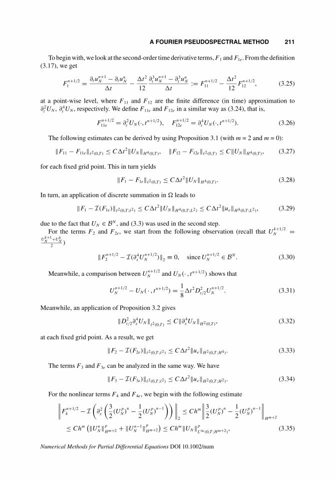
FIG. 1. Discrete L2 numerical errors for ψ = ut and H2 numerical errors for u at T = 4.0, plotted versusN, the number of spatial grid point, for the fully discrete pseudospectral scheme (2.10). The time step sizeis fixed as �t = 10−4. An apparent spatial spectral accuracy is observed for both variables.

in which 0 < P ≤ 1. In more detail, the amplitude A, the wave speed c0 and the real parameterP satisfy

A = 3P 2

2, c0 = (1 − P 2)

1/2. (5.2)

Since the exact profile (5.1) decays exponentially as |x| → ∞, it is natural to apply Fourierpseudospectral approximation on an interval (−L,L), with L large enough. In this numericalexperiment, we set the computational domain as � = (−40, 40). A moderate amplitude A = 0.5is chosen in the test.

A. Spectral Convergence in Space

To investigate the accuracy in space, we fix �t = 10−4 so that the temporal numerical error isnegligible. We compute solutions with grid sizes N = 32 to N = 128 in increments of 8, and wesolve up to time T = 4. The following numerical errors at this final time

‖ψ − ψe‖2, and ‖D2N(u − ue)‖2, (5.3)

are presented in Fig. 1. The spatial spectral accuracy is apparently observed for both u andψ = ut . Due to the fixed time step �t = 10−4, a saturation of spectral accuracy appears with anincreasing N.

B. Second-Order Convergence in Time

To explore the temporal accuracy, we fix the spatial resolution as N = 512 so that the numericalerror is dominated by the temporal ones. We compute solutions with a sequence of time step sizes,�t = T

NK, with NK = 100 to NK = 1000 in increments of 100, and T = 4. Figure 2 shows the



FIG. 2. Discrete L2 numerical errors for ψ = ut and H2 numerical errors for u at T = 4.0, plotted versusNK , the number of time steps, for the fully discrete pseudospectral scheme (2.10). The spatial resolution isfixed as N = 512. The data lie roughly on curves CN−2

K , for appropriate choices of C, confirming the fullsecond-order temporal accuracy of the proposed scheme.

discrete L2 and H2 norms of the errors between the numerical and exact solutions, for ψ = ut

and u, respectively. A clear second-order accuracy is observed for both variables.

VI. CONCLUDING REMARKS

In this article, we propose a fully discrete Fourier pseudospectral scheme for the GB equation (1.1)with second-order temporal accuracy. The nonlinear stability and convergence analysis are pro-vided in detail. In particular, with the help of an aliasing error control estimate (given by Lemma2.1, a �∞(0, T ∗; H 2) error estimate for u and �∞(0, T ∗; �2) error estimate for ψ = ut are derived.Moreover, an introduction of an intermediate variable ψ greatly improves the numerical stabilitycondition; an unconditional convergence (for the time step �t in terms of the spatial grid size h) isestablished in this article, compared with a severe time step constraint �t ≤ Ch2, reported in anearlier literature [10]. A simple numerical experiment also verifies this unconditional convergence,second-order accuracy in time, and spectral accuracy in space.

The authors greatly appreciate many helpful discussions with Panayotis Kevrekidis, inparticular for his insightful suggestion and comments.

References

1. V. S. Manoranjan, A. R. Mitchell, and J. L. Morris, Numerical solutions of the good Boussinesq equation,SIAM Sci Stat Comput 5 (1984), 946–957.

2. V. S. Manotanjan, T. Ortega, and J. M. Sanz-Serna, Soliton and antisoliton interactions in the “good”Boussinesq equation, J Math Phys 29 (1988), 1964–1968.


222 CHENG ET AL.

3. T. Ortega and J. M. Sanz-Serna, Nonlinear stability and convergence of finite difference methods forthe “good” Boussinesq equation, Numer Math 58 (1990), 215–229.

4. B. S. Attili, The Adomian decomposition method for solving the Boussinesq equation arising in waterwave propagation, Numer Methods Partial Differential Equations 22 (2006), 1337–1347.

5. A. G. Bratsos, A predictor-corrector scheme for the improved Boussinesq equation, Chaos SolitonsFractals 40 (2009), 2083–2094.

6. A. G. Bratsos, A second order numerical scheme for the improved Boussinesq equation, Phys Lett A370 (2007), 145–147.

7. R. Cienfuegos, E. Barthélemy, and P. Bonneton, A fourth-order compact finite volume scheme for fullynonlinear and weakly dispersive Boussinesq-type equations, Part I: Model development and analysis,Int J Numer Methods Fluids 51 (2006), 1217–1253.

8. R. Cienfuegos, E. Barthélemy, and P. Bonneton, A fourth-order compact finite volume scheme for fullynonlinear and weakly dispersive Boussinesq-type equations, Part II: Boundary conditions and validation,Int J Numer Methods Fluids 53 (2007), 1423–1455.

9. L. Farah and M. Scialom, On the periodic “good” Boussinesq equation, Proc Am Math Soc 138 (2010),953–964.

10. J. De Frutos, T. Ortega, and J. M. Sanz-Serna, Pseudospectral method for the “good” Boussinesqequation, Math Comput 57 (1991), 109–122.

11. S. Gottlieb and C. Wang, Stability and convergence analysis of fully discrete Fourier collocation spectralmethod for 3-D viscous Burgers’ equation, J Sci Comput 53 (2012), 102–128.

12. F. Linares and M. Scialom, Asymptotic behavior of solutions of a generalized Boussinesq type equation,Nonlinear Anal Theory Methods Appl 25 (1995), 1147–1158.

13. S. Oh and A. Stefanov, Improved local well-posedness for the periodic “good” Boussinesq equation,J Differ Equ 254 (2013), 4047–4065.

14. A. K. Pani and H. Saranga, Finite element Galerkin method for the “good” Boussinesq equation,Nonlinear Anal Theory Methods Appl 29 (1997), 937–956.

15. M. Tsutsumi and T. Matahashi, On the Cauchy problem for the Boussinesq type equation, Math Japonica36 (1991), 371–379.

16. D. Gottlieb and S. A. Orszag, Numerical analysis of spectral methods, theory and applications, SIAM,Philadelphia, PA, 1977.

17. A. Majda, J. McDonough, and S. Osher, The Fourier method for non-smooth initial data, Math Comput32 (1978), 1041–1081.

18. Y. Maday and A. Quarteroni, Legendre and Chebyshev spectral approximations of Burgers’ equation,Numer Math 37 (1981), 321–332.

19. Y. Maday and A. Quarteroni, Approximation of Burgers’ equation by pseudospectral methods, RAIROAnal Numer 16 (1982), 375–404.

20. Y. Maday and A. Quarteroni, Spectral and pseudospectral approximation to Navier-Stokes equations,SIAM J Numer Anal 19 (1982), 761–780.

21. G. Q. Chen, Q. Du, and E. Tadmor, Super viscosity approximations to multi-dimensional scalarconservation laws, Math Comput 61 (1993), 629–643.

22. B.Y. Guo, H. P. Ma, and E. Tadmor, Spectral vanishing viscosity method for nonlinear conservationlaws, SIAM J Numer Anal 39 (2001), 1254–1268.

23. Y. Maday, S. M. Ould Kaber, and E. Tadmor, Legendre pseudospectral viscosity method for nonlinearconservation laws, SIAM J Numer Anal 30 (1993), 321–342.

24. E. Tadmor, Convergence of spectral methods to nonlinear conservation laws, SIAM J Numer Anal 26(1989), 30–44.



25. E. Tadmor, Shock capturing by the spectral viscosity method, Comput Methods Appl Mech Eng 80(1990), 197–208.

26. E. Tadmor, Total variation and error estimates for spectral viscosity approximations, Math Comput 60(1993), 245–256.

27. E. Tadmor, Burgers’ equation with vanishing hyper-viscosity, Commun Math Sci 2 (2004), 317–324.

28. E. Weinan, Convergence of spectral methods for the Burgers’ equation, SIAM J Numer Anal 29 (1992),1520–1541.

29. E. Weinan, Convergence of Fourier methods for Navier-Stokes equations, SIAM J Numer Anal 30(1993), 650–674.

30. B. Y. Guo, A spectral method for the vorticity equation on the surface, Math Comput 64 (1995),1067–1069.

31. B. Y. Guo and W. Huang, Mixed Jacobi-spherical harmonic spectral method for Navier–Stokes equations,Appl Numer Math 57 (2007), 939–961.

32. B. Y. Guo, J. Li, and H. P. Ma, Fourier-Chebyshev spectral method for solving three-dimensional vorticityequation, Acta Math Appl Sin 11 (1995), 94–109.

33. Q. Du, B. Guo, and J. Shen, Fourier spectral approximation to a dissipative system modeling the flowof liquid crystals, SIAM J Numer Anal 39 (2001), 735–762.

34. B. Y. Guo and J. Shen, On spectral approximations using modified Legendre rational functions: appli-cation to the Korteweg-de Vries equation on the half line, Indiana Univ Math J 50 (2001), 181–204,(Special issue: Dedicated to Professors Ciprian Foias and Roger Temam).

35. A. Bressan and A. Quarteroni, An implicit/explicit spectral method for Burgers’ equation, CALCOLO23 (1986), 265–284.

36. Y. Maday and A. Quarteroni, Error analysis for spectral approximation of the Korteweg-de Vriesequation, Math Model Numer Anal 22 (1988), 499–529.

37. B. Pelloni and V. A. Dougalis, Error estimates for a fully discrete spectral scheme for a class of nonlinear,nonlocal dispersive wave equations, Appl Numer Math 37 (2001), 95–107.

38. Z. Deng and H. Ma, Error estimate of the Fourier collocation method for the Benjamin-Ono equation,Numer Math Theory Methods Appl 2 (2009), 341–352.

39. Z. Deng and H. Ma, Optimal error estimates of the Fourier spectral method for a class of nonlocal,nonlinear dispersive wave equations, Appl Numer Math 59 (2009), 988–1010.

40. J. C. López-Marcos and J. M. Sanz-Serna, Stability and convergence in numerical analysis, III: Linearinvestigation of nonlinear stability, IMA J Numer Anal 7 (1988), 71–84.

41. J. Boyd, Chebyshev and Fourier spectral methods, 2nd Ed., Dover, New York, NY, 2001.

42. C. Canuto, M. Y. Hussani, A. Quarteroni, and T. A. Zang, Spectral methods: evolution to complexgeometries and applications to fluid dynamics, Springer-Verlag, Berlin, 2007.

43. J. Hesthaven, S. Gottlieb, and D. Gottlieb, Spectral methods for time-dependent problems, CambridgeUniversity Press, Cambridge, 2007.

44. C. Canuto and A. Quarteroni, Approximation results for orthogonal polynomials in Sobolev spaces,Math Comput 38 (1982), 67–86.

45. G. A. Baker, Error estimates for finite element methods for second order hyperbolic equations, SIAM JNumer Anal 13 (1976), 564–576.

46. A. Baskara, J. S. Lowengrub, C. Wang, and S. M. Wise, Convergence analysis of a second order con-vex splitting scheme for the modified phase field crystal equation, SIAM J Numer Anal 51 (2013),2851–2873.

47. T. Dupont, Galerkin methods for first order hyperbolics: an example, SIAM J Numer Anal 10 (2009),890–899.


224 CHENG ET AL.

48. H. El-Zoheiry, Numerical investigation for the solitary waves interaction of the “good” Boussinesqequation, Appl Numer Math 45 (2003), 161–173.

49. B. Y. Guo and J. Zou, Fourier spectral projection method and nonlinear convergence analysis forNavier-Stokes equations, J Math Anal Appl 282 (2003), 766–791.

50. Q. Lin, Y. H. Wu, R. Loxton, and S. Lai, Linear B-spline finite element method for the improvedBoussinesq equation, J Comput Appl Math 224 (2009), 658–667.

51. F. L. Liu and D. L. Russell, Solutions of the Boussinesq equation on a periodic domain, J Math AnalAppl 192 (1995), 194–219.

52. A. Shokri and M. Dehghan, A not-a-knot meshless method using radial basis functions and predictor-corrector scheme to the numerical solution of improved Boussinesq equation, Comput Phys Commun181 (2010), 1990–2000.

53. E. Tadmor, The exponential accuracy of Fourier and Chebyshev differencing methods, SIAM J NumerAnal 23 (1986), 1–10.

54. C. Wang and S. Wise, An energy stable and convergent finite-difference scheme for the modified phasefield crystal equation, SIAM J Numer Anal 49 (2011), 945–969.

55. A. M. Wazwaz, Constructions of soliton solutions and periodic solutions of the Boussinesq equation bythe modified decomposition method, Chaos Solitons Fractals 12 (2001), 1549–1556.

56. R. Xue, The initial-boundary value problem for the “good” Boussinesq equation on the bounded domain,J Math Anal Appl 343 (2008), 975–995.


A Fourier pseudospectral method for the good Boussinesq ...

Documents

Transcript of A Fourier pseudospectral method for the good Boussinesq ...