Digital Fractional-N Synthesizer Example Achieving Wide Bandwidth and Low Noise

Chun-Ming Hsu

July 21, 2008

Copyright © 2008 by Chun-Ming Hsu

The GRO model and VCO flicker noise model are created by Matt Straayer. All rights reserved.

Table of Contents Setup .................................................................................................................................................. 2 Introduction........................................................................................................................................ 5 Design Goals for an Example Digital Synthesizer ............................................................................ 6 Performing Basic Noise Analysis Using the PLL Design Assistant.................................................. 7 Performing Detailed Noise Analysis Using Matlab......................................................................... 15 Performing Basic Operations within Sue2 and CppSimView ......................................................... 16

A. Opening Sue2 Schematics.................................................................................................... 16 B. Running the CppSim Simulation ......................................................................................... 21

Plotting Time Domain Results......................................................................................................... 23 A. VCO Control Voltage .......................................................................................................... 23 B. Noise Cancellation Signals .................................................................................................. 25 C. GRO signals ......................................................................................................................... 29

Plotting Frequency Domain Results ................................................................................................ 30 Exploring Mismatch within the DAC.............................................................................................. 34 Conclusion ....................................................................................................................................... 38

1

Setup If you have not installed CppSim Version 3 yet, download and install the CppSim package (i.e., download and run the self-extracting file named setup_cppsim3.exe) located at:

http://www.cppsim.com/

Upon completion of the installation, you will see icons on the Windows desktop corresponding to the PLL Design Assistant, CppSimView, and Sue2. Please read the “CppSim (Version 3) Primer” document, which is at the same web address, to become acquainted with CppSim and its various components. Now, create a folder called Import_Export under C:\CppSim. Download wb_digital_synthesizer.tar.gz to C:\CppSim\Import_Export. Launch Sue2 by clicking Sue2 icon on your desktop. Click tools and then Library Manager.

2

You should see the CppSim Library Manager as above. Click on Import Library Tool. You should see:

3

Enter the Destination Library, Source Directory, and Source File/Library as below:

Press Import. After the library is imported, the window looks like:

4

You need to restart Sue2 before the new library can be seen. Finally, you are encouraged to read the manual “PLL Design Using the PLL Design Assistant Program”, which is also located at http://www.cppsim.com/, to obtain more information about the PLL Design Assistant. Introduction Recent dramatically increasing application of the fractional-N frequency synthesizer to wireless communication has made the fractional-N frequency synthesizer a hot research area. On the one hand, the need of a wider-bandwidth fractional-N synthesizer has inspired researchers to develop phase noise cancellation techniques to avoid the tradeoff between the noise performance and synthesizer bandwidth. On the other hand, the continuing development of deep submicron CMOS process has initiated people’s interest in all-digital phase locked loop (PLL), which not only leverages the high-speed digital capability available in a deep submicron process to build a compact, configurable loop filter but also avoids the problems conventional charge-pump PLL may encounter, like high variation and leakage current. A digital fractional-N frequency synthesizer is proposed which leverages a noise-shaping time-to-digital converter (TDC) and a simple quantization noise cancellation technique to achieve low phase noise with a wide PLL bandwidth of 500 kHz. [1]. Fig. 1 shows a block diagram of the proposed synthesizer. High-resolution digital phase detection is performed with a gated ring oscillator (GRO) time-to-digital converter presented in [2]. Another interesting component of the architecture is an asynchronous frequency divider which avoids the divide-value dependent delay at its output. In addition, in contrast to previous digital PLL implementations, the digitally-controlled oscillator (DCO) is implemented as a conventional LC voltage-controlled oscillator (VCO) with coarse and fine varactors which are controlled by two passive 10-bit, 50 MHz digital-to-analog converter (DAC) structures. This tutorial will focus on simulation and experimentation with relevant design variables of this architecture. We recommend first reading [1,2] to understand the synthesizer architecture and basic idea of the GRO TDC. In addition, we also recommend the other two related tutorials to fractional-N synthesis, “Fractional-N Frequency Synthesizer Design Using The PLL Design Assistant and CppSim Programs” and “Design of a Wideband Fractional-N Frequency Synthesizer Using CppSim”. Both of them are available at

http://www.cppsim.comAfter finishing this tutorial, you are also encouraged to read [3,4] to further understand the proposed technique. [1] C.-M. Hsu, M. Straayer, and M. Perrott, “A Low-Noise Wide-BW 3.6GHz Digital Fractional-N Frequency Synthesizer with a Noise-Shaping Time-to-Digital Converter and Quantization Noise Cancellation” , ISSCC Dig. Tech. Papers, Feb. 2008. [2] M. Straayer and M. Perrott, “An efficient high-resolution 11-bit noise-shaping multipath gated ring oscillator TDC,” VLSI Symp. Dig. Tech. Papers, pp 82-83, June 2008.

5

[3] C.-M. Hsu, M. Straayer, and M. Perrott, “A Low-Noise Wide-BW 3.6GHz Digital Fractional-N Frequency Synthesizer with a Noise-Shaping Time-to-Digital Converter and Quantization Noise Cancellation” , IEEE Journal of Solid-State Circuits, to be published in Dec. 2008. [4] C.-M. Hsu, “Techniques for high-performance digital frequency synthesis and phase control,” Ph.D. dissertation, Mass. Inst. Technol., Cambridge, MA 2008.

Figure 1: Proposed ΔΣ Fractional-N Synthesizer [1].

Design Goals for an Example Digital Synthesizer As a target application for the digital synthesizer, we set the following specifications:

• PLL specifications

o 500kHz closed loop synthesizer bandwidth o Order: 2 (We want a simple implementation) o Filter Shape: Butterworth o Parasitic Pole at 3MHz (helps to attenuate high frequency noise. This is a standard

noise reduction “trick” used in synthesizer design) o Type: 2 with fz/fo = 1/8 o 3.6GHz output frequency

6

o 50MHz reference frequency

• Noise Specifications

o No worse than -100dBc/Hz in-band noise. (In-band noise is noise within the loop

bandwidth) o -150dBc/Hz VCO phase noise at 20MHz offset from the carrier o Minimal residual spurs present in the output.

These design goals would allow the synthesizer to be used as a direct modulated GSM transmitter if the VCO output is divided by four. Below is the GSM 900MHz phase noise mask specifications, as well as the equivalent noise performance required by a 3.6GHz signal that is divided down to generate the 900MHz signal, assuming a noiseless division is performed. 100

kHz 200 kHz

250 kHz

400 kHz

600 kHz

1.8 MHz

3.0 MHz

6.0 MHz

10 MHz

20 MHz

900 MHz

-52.3 dBc/Hz

-82.8 dBc/Hz

-85.8 dBc/Hz

-112.8 dBc/Hz

-112.8 dBc/Hz

-121 dBc/Hz

-123 dBc/Hz

-129 dBc/Hz

-150 dBc/Hz

-162 dBc/Hz

3.6 GHz

-40.3 dBc/Hz

-70.8 dBc/Hz

-73.8 dBc/Hz

-100.8 dBc/Hz

-100.8 dBc/Hz

-109 dBc/Hz

-111 dBc/Hz

-117 dBc/Hz

-138 dBc/Hz

-150 dBc/Hz

Performing Basic Noise Analysis Using the PLL Design Assistant A. VCO Noise Requirement We first review the basic functions of PLL Design Assistant quickly by checking the VCO noise requirement. Open the PLL Design Assistant and put in the parameter values, as shown below. By clicking on the Apply button, you should get the same resulting phase noise plot. Note that the resulting rms jitter of 142fs is also shown.

7

To compare the noise with the specification, we have created a text file as follows:

8

You should be able to find this text file, gsm_mask.txt, in C:\CppSim\SimRuns\wb_digital_ synthesizer\dsynth_top1. Load the text file to PLL Design Assistant by clicking Templates and Load Mask Data. Click Apply again, you should obtain the same result as:

B. TDC Noise Impact on Digital Synthesizer Performance

We now explore the TDC resolution requirement to meet our noise specification. The in-band phase noise floor due to the finite resolution of a non-noise-shaping TDC can be calculated with the following equation:

10log(1/T·(2π·N)2· (1/12·Td2))

, where N, T, Td are divider ratio, reference period, and TDC resolution, respectively. Set detector noise to -95 dBc/Hz, which corresponds to a TDC resolution of 20ps and then click Apply again. You will see the resulting noise is too high to meet the specification. You can now try to meet the specification by decreasing the detector noise value until -105dBc/Hz (shown below), which needs a TDC resolution of 6ps. Note that this fine resolution is still not easy to implement with today’s process.

9

In contract, GRO-TDC achieves lower PLL noise by first-order shaping the quantization noise to higher frequencies. The shaped noise is then attenuated by the PLL loop response. Due to the limitation of PLL Design Assistant, we are not able to add the shaped quantization noise to this model. To understand the GRO performance better, a MATLAB script (explained later) was created to calculate the resulting noise including the GRO quantization noise, and the result is shown below. Note that the GRO noise is lower than the VCO noise at high frequencies.

103 104 105 106 107-180

-160

-140

-120

-100

-80

-60

-40

dBc/

Hz

foffset

VCO NoiseGRO NoiseOverall Noise

10

The MATLAB code also includes 1/f and thermal noise those limit low-frequency performance. We can include this noise in PLL Design Assistant by changing the detector noise to [-120 150e3 -10]. (The noise floor is –120dBc/Hz. The slope and flicker noise corner are –10dB/dec and 150kHz, respectively.). The resulting plot is shown below.

Notice that the result got from PLL Design Assistant is very close to the one from MATLAB. It is because the shaped and attenuated GRO quantization noise is so low that we don’t lose much accuracy even without including it in our model. In addition, from this result, it is realized that GRO-TDC achieves much better performance than conventional non-noise-shaping TDC given the same resolution of 6ps. We now obtain about 10dB margin at 400-kHz by utilizing a GRO-TDC. The rms jitter is also reduced from 341fs to165fs. C. Divider Quantization Noise Impact on Digital Synthesizer Performance The other important noise source is the divider quantization noise. In the PLL Design Assitant window, enter a 3rd order noise transfer function into the S-D noise box by first clicking the “On” button and entering [1 -3 3 -1] into the parameter box, as depicted below. Press Apply.

11

Note that the quantization noise associated with the 3rd order ΔΣ modulation ruins noise performance! The standard way to combat this noise would be to reduce the synthesizer bandwidth. You can experiment with this using the PLL Design Assistant. We will not do so here because reducing the bandwidth violates our stated goal of achieving a 500kHz bandwidth. We can improve the noise performance by applying phase noise cancellation technique. The question is how much residual noise we can tolerate without violating our specification. To

12

investigate it, we change the noise transfer function from [1 -3 3 -1] to 0.1*[1 -3 3 -1], meaning 10% of this noise is left after noise cancellation.

Note that the quantization noise associated with the 3rd order ΔΣ synthesizer is now below the VCO noise, and the increase in rms jitter is less than 1fs. You can also try a 2nd order ΔΣ modulator. It will be realized that by using a 2nd order modulator, a more accurate noise cancellation (~95%) is necessary to obtain compatible performance.

13

Now, let’s zoom in the phase noise around 20MHz by left clicking the phase noise plot. As shown below, the total noise is slightly higher than -150dBc/Hz. The lesson we learn here is we should have reserved some margin for the VCO noise specification. Decreasing the VCO noise from -150dBc/Hz to -151dBc/Hz will solve this problem. However, please notice that a three to five dB margin is necessary in practice.

D. Other Noises There are another three noises not added to the model yet. They are:

• Coarse-Tune DAC thermal noise • Fine-Tune DAC thermal noise • Fine-Tune DAC 1st order ΔΣ quantization noise

Again, because the limitation of PLL Design Assistant, these three noises are not able to be included into our model yet.

E. Resulting open loop parameters According to the specified bandwidth and filter type, PLL Design Assistant automatically calculates three open loop parameters: K, fp (pole position), fz (zero position). As plotted below, these parameters are shown on the left-lower corner of PLL Design Assistant GUI. These values will be used in the CppSim model as well as a MATLAB script for detailed noise analysis.

14

. Performing Detailed Noise Analysis Using Matlab As mentioned above, some of the noise sources in the proposed synthesizer cannot be included in PLL Design Assistant. A MATLAB script was therefore created to investigate the impact of these noises in more detail. This MATALB script, noise_dsynth.m, as well as another short script, par_calc.m, can be found in

C:\CppSim\SimRuns\wb_digital_synthesizer\dsynth_top1. We now plot the complete PLL output phase noise with the help of these scripts. Details of this noise model can be found in [4]. First, open the script par_calc.m. On the top of this script are the three parameters K, fp, and fz obtained from PLL Design Assitant. Following these three parameters are a few other parameters determined through circuit design. This script should return three parameters K1=127.3, K2=0.0513, and alpha=0.8961, which are needed in the script noise_dsynth.m. Please refer [4] for details of these parameters.

15

Now open the script noise_dsynth.m and enter the three parameters we just got on lines 44, 45, and 46, respectively. (The numbers have been entered for you.) Run the script and you should see a phase noise plot similar to the one below:

103 104 105 106 107-180

-160

-140

-120

-100

-80

-60

-40

dBc/

Hz

foffset

VCO NoiseFinepath ΣΔ Quantization NoiseFine-tune DAC ThermalCoarse-tune DAC ThermalDivider Noise (1% left)GRO NoiseRef NoiseClose-loop Noise

Note that all of the noise sources, except the thermal noise of the coarse-tuning DAC, are considerably lower than the VCO noise. Although the thermal noise from the coarse-tuning DAC is slightly higher than the VCO noise at intermediately frequencies, the overall PLL noise can still achieve < -100 dBc/Hz within the loop bandwidth. More details about the noise analysis and design considerations can be found in [4]. Performing Basic Operations within Sue2 and CppSimView In this section, the user will be guided through basic tasks such as opening the digital synthesizer example within the Sue2 schematic editor and running CppSim simulations.

A. Opening Sue2 Schematics • Click on the Sue2 icon to start Sue2, and then select the wb_digital_synthesizer library

from the schematic listbox. The schematic listbox should now look as follows: •

16

• Scroll down and click on the dsynth_top1 schematic. The behavioral model of the digital synthesizer is shown below:

17

• The model is setup in a way that you can bring the three loop filter parameters K, fp, fz obtained with PLL Design Assistant to CppSim easily. They are highlighted in the figure above.

• There are several key blocks in the system:

18

o dsynth_detector: This is the phase detector structure using the GRO-TDC. Select the dsynth_detector icon within the dsynth_top1 schematic, and then press e to descend into it. You will see the schematic depicted below. In addition to the GRO and its supporting blocks, this schematic includes two other important blocks:

dsynth_divider_ds: This block describes the proposed divider architecture in [1].

dsynth_correlation: This block describes the proposed all-digital correlation loop in [1].

You can descend into these blocks to see the schematic. Press Ctrl+e to return to the previous level.

19

o dsynth_filter: This blocks describes the digital filter, consisting of a coarse-

tune filter and a fine-tune filter. Descend into this block. The digital outputs of both filters are converted into analog signals by two DACs (dsynth_dac). Description of this DAC structure can be found in [1]. The dual port characteristic of the VCO is modeled with the following equation: Vctrl=Vcoarse+Vfine*var_ratio, where Vcoarse and Vfine are the output of the coarse and fine DACs, respectively, and the coefficient var_ratio (default value is 1/16) represents the ratio between the fine and coarse varactors.

o dsynth_vco: This is a VCO model including flicker noise. o accum_and_dump: This block is used to decimate the output data so that very

long simulations can be quickly plotted. • The key signals present in the system are:

o noiseout_filt: The filtered control voltage used to control the VCO. This signal

will be used to calculate and plot the synthesizer output spectrum.

• Descend into dsynth_detector. Key signals within this block include:

o x: This signal is an accumulated version of the ΔΣ quantization noise used to estimate the phase error due to the dithering action of the divider.

o scale: This is the output of the correlation loop used as a scaling factor to adjust

the magnitude of x.

20

o y: This signal equals to x times scale.

o u: This is a scaled and unwrapped version of the GRO output. This signal

represents the phase error before quantization noise cancellation is performed.

o e: This signal represents the phase error after quantization noise cancellation is performed. The relation between e, u ,and y is e=u+y.

o gro_out_d: This is the GRO output signal.

o mult: GRO gain is coarsely normalized with the multiplier following it. Thus,

the signal mult is a scaled version of GRO output.

o unwrap: During the frequency acquisition cycle, the GRO output may wrap similarly to cycle slipping of a tri-state PFD. An unwrap signal is generated to eliminate the effect of the wrapping action such that the overall phase detector has an almost-linear transfer function.

• Descend into dsynth_filter. Key signals within this block include:

o vcoarse: This is the coarse-path DAC output that controls the coarse varactor in

the VCO. o vfine: This is the fine-path DAC output that controls the fine varactor in the

VCO.

B. Running the CppSim Simulation

• Within Sue2, Click on Tools and then CppSim Simulation. The CppSim Simulation Window should appear as shown below.

21

• Double click on the Edit Sim File button. An emacs window should appear that indicates that the number of simulation steps, num_sim_steps, is set to 48e7 and the timestep, Ts, is set to 5e-12. You can close the emacs window if you like.

• Click on the Compile/Run button to launch the simulation.

• Click on the CppSimView icon on your desktop to start the CppSim viewer. (You

don’t have to wait until the simulation is completed!) • Click on the No Output File radio button and select test.tr0 as the output file. • Click on the No Nodes radio button to load in the simulated signals. CppSimView

should now appear as shown below.

22

Plotting Time Domain Results Given the above simulation, we will now examine some of the key signals in the system during normal operation.

A. VCO Control Voltage • In the CppSimView window, double-click on signals xi9_vcoarse and xi9_vfine. You

should see the waveforms shown below.

23

• As described in [1], both vcoarse and vfine are first brought to VDD/2 (0.75V) when synthesizer frequency changes. At t=3μs, the coarse filter is enabled and vcoarse is allowed to change, while vfine is frozen at VDD/2 during this period. At t=15μs, the coarse filter and vcoarse are frozen, but the fine filter is enabled such that vfine can vary to control the VCO frequency. The time coarse filter and fine filter are enabled can be changed in dsynth_top1 schematic.

• We see that, after some simulation startup conditions, the VCO control voltages settle

to a steady-state value.

• In the CppSimView window, click on Zoom. The waveform window will now look as below.

• Click on the Zoom button in the waveform window, and then zoom in several times in the 5μs to 25μs range until you observe the waveform below:

24

• Notice there is a disturbance on vfine at t=15 μs. It is because we switch from the coarse filter to fine filter at this point. Due to the high resolution of the coarse DAC, vfine doesn’t have to move much. As a result, the disturbance is small, and vfine stays around VDD/2.

• Note that vcoarse and vfine are changing over time even after the loop locks, which is

due to the random noise sources present in the simulation. However, the variation of control voltage is bounded within a range after t=20 μs, so we can claim the locking time of this PLL is about 20 μs.

B. Noise Cancellation Signals • In the CppSimView window, double-click on signals xi4_e, xi4_u, xi4_y, xi4_x, and

xi4_scale. You should see the waveform shown below. In the beginning, the scale signal is reset to zero, meaning the phase cancellation function is disabled. Since y equals to zero, e is exactly the same as u. The correlation loop and noise cancellation begins to function at t=15μs, so you can see e becomes much less noisier after t=15μs.

25

• Zoom in several times in the 15.1μs to 36μs range until you observe the waveform

below. You should see the scale signal starts to increase from one until it settles around 1.2. Signal e becomes the sum of u and y (signs of u and y are opposite), and the magnitude of e keeps on decreasing as scale is increasing. It is indicated from this figure that the settling time of the correlation loop is around 10μs. Notice that scale doesn’t keep a constant after the loop settles, but the variation is small. Recall that we can tolerate 10% residual noise, so this variation is not an issue.

26

27

• Zoom in several times to focus on the time region around 15.3μs. Notice that the signals u and y seem similar but different in magnitude and sign (Ignore the dc component in u, which will be taken away afterwards). Their magnitudes are different because the correlation loop hasn’t settled yet, and thus e is highly correlated to x.

28

• Zoom out several times and zoom in several times again to focus on the time region

around 29μs. Notice that after the correlation loop settles, e becomes smaller and less correlated to x. This is because the noise left in e is dominated by GRO quantization noise instead of the ΔΣ noise.

C. GRO signals

• In the CppSimView window, double-click on signals xi4_gro_out_d, mult, unwrap, and u. Zoom in to focus on the time region around 4μs. You should see the waveforms shown below.

29

• Notice that gro_out_d and mult wrap. However, by summing unwrap and mult together, the resulting signal u doesn’t wrap such that the overall phase detector behaves having an almost-linear transfer function. (Signal u wraps before t=3μs because unwrapping function is disabled when t<3μs.)

Plotting Frequency Domain Results

• We will now observe the synthesizer output spectrum.

30

• First, click on the test.tr0 radio button, and select test_noise.tr0 from the file list. • Then click the No Nodes radio button. • Next, Click on the plotsig(…) radio button and select

plot_pll_phasenoise(x,f_low,f_high,’nodes’) from the list. • Next, click the nodes radio button. • Edit the plot_pll_phasenoise command so that f_low=5e3, f_high=80e6, and

‘nodes’=noiseout_filt. The result should appear as below.

31

• We observe that the spectrum appears to roughly match the calculated values using the

PLL Design Assistant.

Please be aware that if the complete simulation hasn’t finished yet, the spectrum you see may be noisier than the one appears here. You can press Load and Replot bottom to update simulation results. If necessary, you can also increase the number of simulation steps in your test.par to obtain a better plot than the one shown here. Of course, it will take a longer simulation time.

32

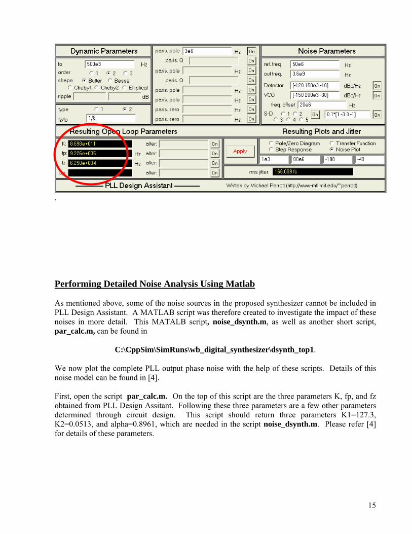
Now, let’s compare this time-domain simulation result with the predicted phase noise using MATLAB. You should be able to find another MATALB script, comp_psd.m, in C:\CppSim\SimRuns\wb_digital_synthesizer\dsynth_top1. Run this script and you should get a plot similar to the one below.

103 104 105 106 107-180

-170

-160

-150

-140

-130

-120

-110

-100

-90

-80Simulated Output Spectrum of Synthesizer

Frequency Offset from Carrier (Hz)

Out

put S

pect

rum

(dB

c/H

z)

33

Now open the script noise_dsynth.m and run it again. You should see the CppSim plot overlapped with the calculated performance, as shown below. Notice that the simulation results using CppSim matches the calculated noise quite well.

103 104 105 106 107-180

-160

-140

-120

-100

-80

-60

-40Simulated Output Spectrum of Synthesizer

foffset

dBc/

Hz

Measured NoiseVCO NoiseFinepath ΣΔ Quantization NoiseFine-tune DAC ThermalCoarse-tune DAC ThermalDivider Noise (100% left)GRO NoiseRef NoiseClose-loop Noise

Exploring Mismatch within the DAC In this section, we explore non-idealities associated with the DAC, and observe their impact on the overall noise performance. The primary sources of mismatch within the DAC are magnitude mismatch between the unit element resistors and capacitors. As detailed in [1], the first section of the DAC is comprised of 32 unit resistor elements, while the second section of the DAC is comprised of 32 unit capacitor elements. Although monotonicity can be guaranteed, mismatch between the unit elements results in nonlinearity of the DAC transfer function. Since the quantization noise of the 1st-order ΔΣ modulator before the DAC sees the nonlinearity before being filtered, it may be folded back to in-band. Instead of using dynamic-element-matching technique, which may result in undesired tones, the 10-bit DAC structure is intended to reduce the magnitude of the quantization noise and thus the folded amount. We explore the impact of this mismatch in the behavioral model.

34

• Descend into dsynth_filter and zoom in until you can see the parameters of the DAC

clearly.

• The mismatch is set using a Gaussian profile that has a user specified standard deviation. The standard deviation of the resistors and capacitors are set by the mmstddev_r and mmstddev_c control parameters, respectively. The value mm is defined in your test.par. Change it from 0.00 to 0.05, which corresponds to a standard deviation of 5% mismatch between the unit elements. The value of the standard deviation can be obtained in process document or by Monte Carlo simulation with Hspice or Spectre.

• Save the schematic.

• Run the simulation and plot the phase noise again. You should see the plot shown as

below:

We see that unit element mismatch appears to have minimal impact on phase noise performance.

• If being interested, you can change different standard deviation values. An alternative

method is to use the alter function in CppSim. For example, open test.par and scroll down to the end of the file. Type mm=0:0.025:0.05 after alter:, meaning we will sweep mm from 0 to 0.05 with a step of 0.025. CppSim will generate three sets of output files

35

corresponding to various mm values. This simulation may take a long time (You can decrease number of simulation steps to save time). After it is done, plot phase noise from different files and compare them.

• If being interested, you can change to different output frequencies. Again, open your

test.par and scroll down to global param:. The output frequency is set to 50MHz*in_gl. The default value of in_gl is 72.3, so the synthesizer will generate an output frequency of 50MHz*72.3=3.615GHz. You can change in_gl to obtain a different frequency.

The last experience we will do here is to run the simulation several times given the same mismatch standard deviation:

• Open your test.par and scroll down to global param:. Notice the global parameter sim_run=0. Make sure you also set mm=0.05.

• Change your alter command to Alter: sim_run=1:1:10. Reduce the simulation steps by

four to save simulation time. Your test.par file should look like

36

• Save your test.par and launch the simulation. This setup will run the simulation ten times. Each time, different resistor or capacitor values with a standard deviation of 0.05 will be assigned to each unit element. This experience allows us to check the yield of the design.

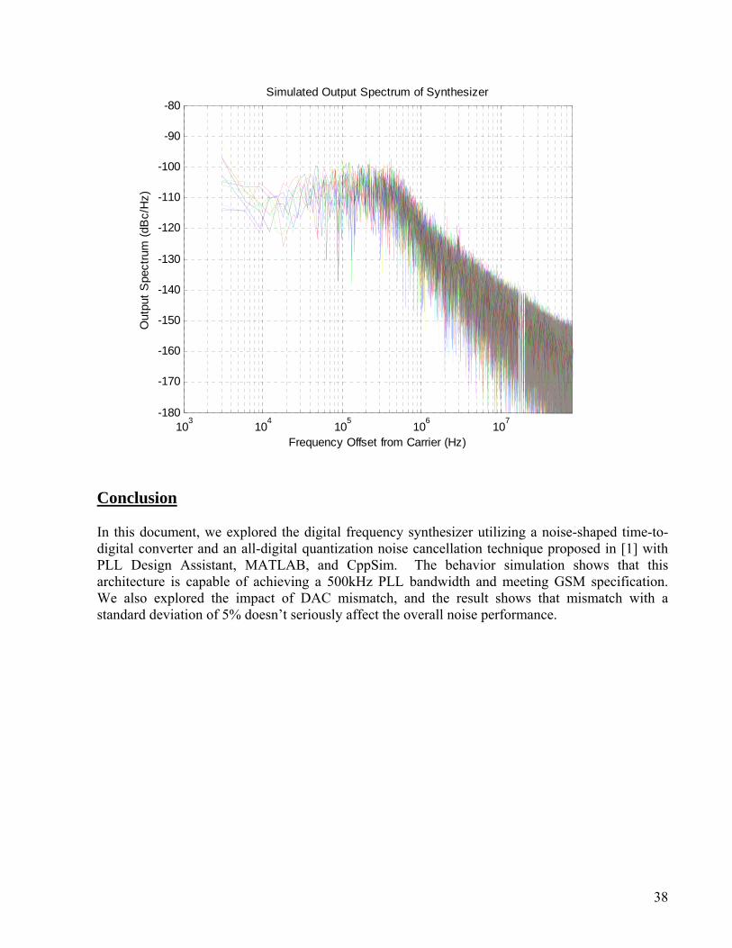
• After the simulation is completed, check each phase noise plot. You should see this mismatch value does not impact the overall noise performance seriously. Advanced user can use MATLAB to plot all of the results together as shown below. Note that this plot looks noisier than the previous ones because the number of simulation steps is reduced by a factor of four to save time.

37

103 104 105 106 107-180

-170

-160

-150

-140

-130

-120

-110

-100

-90

-80Simulated Output Spectrum of Synthesizer

Frequency Offset from Carrier (Hz)

Out

put S

pect

rum

(dB

c/H

z)

Conclusion In this document, we explored the digital frequency synthesizer utilizing a noise-shaped time-to-digital converter and an all-digital quantization noise cancellation technique proposed in [1] with PLL Design Assistant, MATLAB, and CppSim. The behavior simulation shows that this architecture is capable of achieving a 500kHz PLL bandwidth and meeting GSM specification. We also explored the impact of DAC mismatch, and the result shows that mismatch with a standard deviation of 5% doesn’t seriously affect the overall noise performance.

38