Controlled Variables: Psychology as the Center...

Controlled Variables: Psychology as the Center Fielder Views It

Richard S. Marken

The American Journal of Psychology, Vol. 114, No. 2. (Summer, 2001), pp. 259-281.

Stable URL:

http://links.jstor.org/sici?sici=0002-9556%28200122%29114%3A2%3C259%3ACVPATC%3E2.0.CO%3B2-2

The American Journal of Psychology is currently published by University of Illinois Press.

Your use of the JSTOR archive indicates your acceptance of JSTOR's Terms and Conditions of Use, available athttp://www.jstor.org/about/terms.html. JSTOR's Terms and Conditions of Use provides, in part, that unless you have obtainedprior permission, you may not download an entire issue of a journal or multiple copies of articles, and you may use content inthe JSTOR archive only for your personal, non-commercial use.

Please contact the publisher regarding any further use of this work. Publisher contact information may be obtained athttp://www.jstor.org/journals/illinois.html.

Each copy of any part of a JSTOR transmission must contain the same copyright notice that appears on the screen or printedpage of such transmission.

The JSTOR Archive is a trusted digital repository providing for long-term preservation and access to leading academicjournals and scholarly literature from around the world. The Archive is supported by libraries, scholarly societies, publishers,and foundations. It is an initiative of JSTOR, a not-for-profit organization with a mission to help the scholarly community takeadvantage of advances in technology. For more information regarding JSTOR, please contact [email protected].

http://www.jstor.orgTue Sep 11 11:25:41 2007

http://links.jstor.org/sici?sici=0002-9556%28200122%29114%3A2%3C259%3ACVPATC%3E2.0.CO%3B2-2

http://www.jstor.org/about/terms.html

http://www.jstor.org/journals/illinois.html

Controlled variables: Psychology as the center fielder views it RICHARD S. MARKEN Life Learning Associates

Perceptual control theory (PCT) views behavior as the control of perception. The central explanatory concept in PCT is the controlled variable, which is a perceived aspect of the environment that is brought to and maintained in states specified by the organism. According to PCT, understanding behavior is a matter of discovering the variables that organisms control. But the possible existence of controlled variables has been largely ignored in the behavioral sciences. One notable exception occurs in the study of how baseball outfielders catch fly balls. In these studies it is taken for granted that the fielder gets to the ball by controlling some visual aspect of the ball's movement. This article describes the concept of a controlled variable in the context of research on fly ball catching behavior and shows how this concept can contribute to our understanding of behavior in general.

The publication of John B. Watson's (1913) Psychology as the Behaviorist ViausIt signaled the beginning of an era of psychological research dom- inated by the search for controlling variables, the variables that control behavior. Behavioral psychologists started looking for these variables in the organism's environment. Cognitive psychologists are now looking for these variables in the organism's mind (or brain). But in both cases the search is for controlling variables, the variables that cause organisms to behave as they do. This preoccupation with controlling variables may be one reason psychologists have paid so little attention to a theory of behavior that focuses on the variables that are controlled by behavior. The theory is called perceptual control theory (PCT), and its basic assumption is that behavior is organized around the control of perceptual variables (Powers, 1973a).

Purpose and control

PCT was developed to explain the purposeful behavior of organisms (Marken, 1990). Purposeful behavior involves producing consistent results in a world where unpredictable disturbances make such consistency highly unlikely (Old Faithful notwithstanding). For example, a person sipping tea is producing a consistent result-the sips-despite

AMERICAN JOURNAL OF PSYCHOLOGY Summer 2001, Vol 114, No. 2, pp. 259-281 Q 2001 by the Board of Trustees of the University of Illinois

260 MARKEN

unpredictable disturbances, such as head movements, that change the relative location of cup and lips. Sipping tea is a purposeful behavior.

PCT is based on the realization that purposeful behavior, like that of the tea drinker, is equivalent to the controlling done by artificial control systems, such as a thermostat. In both cases, a consistent result is produced despite unpredictable disturbances that should produce in- consistency. The thermostat produces a consistent room temperature despite unpredictable changes in outdoor air temperature; the tea drinker produces consistent sips despite unpredictable changes in the relative location of cup and lips.

Control systems act to bring variable aspects of the environment to preselected states while protecting these variables from the effects of disturbance. This process is called control. The variable aspects of the environment that a system controls are called controlled variables; room temperature and distance from cup to lips are controlled variables. The purposeful behavior of a control system, whether it is living (like the tea drinker) or artificial (like the thermostat), is organized around controlled variables. Control theory explains how a control system acts to keep these variables under control. PCT is the application of control theory to understanding the purposeful behavior of control systems in general and living control systems in particular.

Control theory

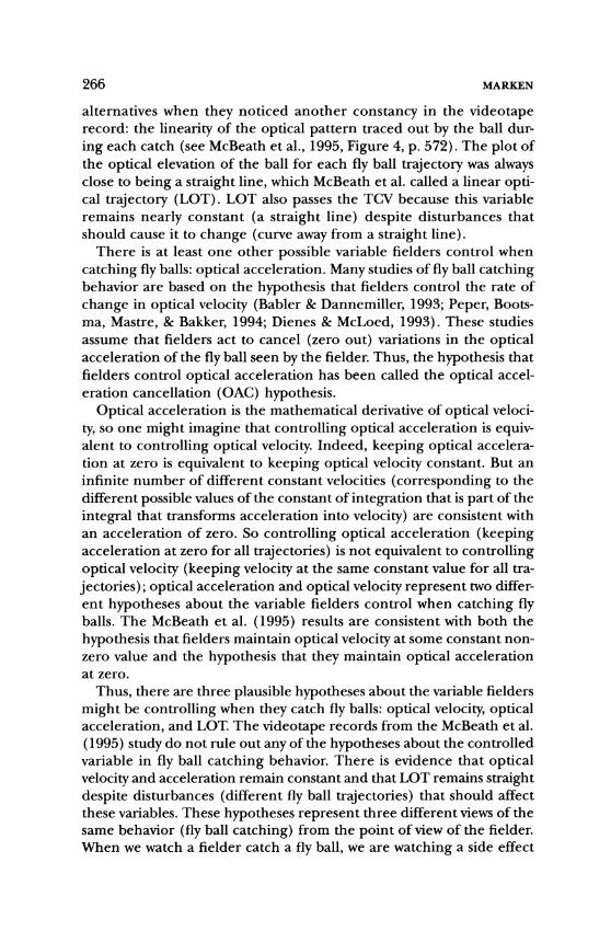
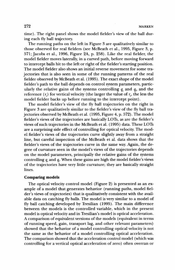
Control theory describes the organization of systems that can control variables such as room temperature or the distance from cup to lips. A basic control system is shown in Figure 1.The upper part of the figure

I m

Input Output Function Function 1

Environment

Figure 1 . A basic control system

261 CONTROLLED VARIABLES

represents the control system itself; the lower part of the figure represents the system's environment. The most important aspect of the environment is the controlled variable (q,). The thermostat's controlled variable is room temperature; the tea drinker's controlled variable is distance from cup to lips.

The state of the controlled variable is influenced by other variables in the environment, which include independent influences on qi, called disturbances (4,and the actions of the control system itself, called outputs ( q J . Room temperature is influenced by disturbances, such as variations in outdoor air temperature, and by the outputs of the thermostat itself: the variations in the amount of heat generated by the furnace. The distance from cup to lips is influenced by disturbances, such as the variations in the location of the mouth, and by the outputs of the tea drinker herself: the forces exerted on the cup as it is lifted to the

'lips. The controlled variable is represented inside the control system as a

perceptual signal (p) .This perceptual signal is the output of a transduc- er, called the input function, which converts variable aspects of the control system's environment into signals inside the control system itself. The perceptual signal is continuously compared to a reference signal (r) that specifies the target or intended value of the perceptual signal. The comparator computes the difference between the reference and perceptual signals (r- p) ;this difference is the error signal ( e ).The error signal causes, via the output function, the outputs that have effects on the controlled variable.

The variables in a control system trace out a closed loop of cause and effect. Variables in any part of this loop have effects that feed back on themselves. Moreover, the feedback effects of variables in this loop tend to cancel themselves out, a process called negative feedback. The result of this negative feedback process is that the perceptual signal is brought to and maintained at a fixed or variable reference state by the outputs of the system, protected from the effects of disturbance. So the behavior of a negative feedback control system is properly described as control of perception (Powers, 1973a). When a perception is controlled, the environmental correlate of that perception-the controlled variable-is also controlled.

Controlled variables and behavior

A control system can produce some rather complex-looking behavior. For example, the thermostat turns the furnace on and off for varying amounts of time, producing a complex pattern of furnace-actuating behavior. One approach to understanding this behavior is to try to discover its causes. But control system behavior cannot be understood in cause-effect terms because cause-effect relationships ignore the

262 MARKEN

possible existence of variables that the system might be controlling (Marken, 1993; Powers, 1973b). For example, the apparent cause-effect relationship between window opening and furnace actuating does not reveal the fact that the thermostat is controlling room temperature. The same cause-effect relationship would be seen if the thermostat were controlling some other variable, such as relative humidity. Indeed, this cause-effect relationship would be seen even if the thermostat were controlling nothing at all; furnace actuating behavior could be caused by a switch that is turned on when the window is opened and off when it is closed.

Control system behavior can be properly understood only in terms of controlled variables. Once you know that the system is controlling a particular variable, you can predict its behavior with great accuracy. Much of the apparent complexity of control system behavior results from the fact that the system's outputs mirror the effects of disturbances to the controlled variable (Powers, 1978). Complex behavior is seen in environments where disturbances produce complex effects on controlled variables. For example, a complex pattern of furnace-actuating behavior is seen in an environment where disturbances (such as win- dows opening and closing, people entering and leaving the room) produce a complex pattern of effects on the variable the thermostat is controlling: room temperature. The discovery of controlled variables (such as room temperature) therefore can provide a simple and elegant ex- planation of what may appear to be very complex behavior.

Noticing controlled variables

Controlled variables are the central feature of purposeful behavior, but they have gone largely unnoticed in the behavioral sciences. This may be because controlled variables are difficult to notice under ordinary circumstances. For example, if you did not already know that a thermostat controls room temperature, it would be difficult to notice that room temperature is being controlled by the thermostat's behavior. What is noticed is the thermostat's reaction to stimuli such as a cold blast of air from an opened window. What is not noticed is the controlled variable itself, the room temperature, which changes little.

Controlled variables are hard to notice under ordinary circumstances precisely because these variables do not react to stimuli (disturbances). It is harder to notice something that does not happen (such as the almost nonexistent response of the controlled variable to disturbances) than something that does (such as the control system's marked response to any disturbance to the controlled variable, a response that prevents the disturbance from having much effect on the controlled variable).


Although it is hard to notice controlled variables, it is not impossible. A good approach to noticing controlled variables is to try to look at behavior from the point of view of the control system itself. For example, if you did not know that the thermostat was controlling room temperature you might be able to figure it out by asking yourself what the thermostat might be trying to perceive by turning the furnace on shortly after the window is opened and off shortly after it is closed. Putting yourself in the thermostat's shoes (or housing) might help you realize that the thermostat is trying to perceive a constant room temperature; room temperature is a controlled variable.

Similarly, you could put yourself into the paws of Pavlov's dog and ask what you might be trying to perceive by salivating when dry food is placed in your mouth. Perhaps you are trying to feel food that is wet, smooth, and easy to swallow rather than food that is dry, sticky, and difficult to swallow; the texture of the food might be a controlled variable. Or you could put yourself behind the nose of Skinner's rat and ask what you might be trying to perceive by quickly repeating the bar press that just gained you a food pellet. Perhaps you are trying to perceive food pellets arriving as quickly as possible; the rate of food pellet delivery might be a controlled variable.

The test for the controlled variable

When behavior is viewed in terms of controlled (rather than controlling) variables, an important question immediately presents itself: How do you determine whether a variable that seems to be under control actually is under control? How do you know whether the thermostat is controlling room temperature? How do you know whether Pavlov's dog is controlling the texture of the food placed in its mouth? How do you know whether Skinner's rats are controlling the rate of food pellet delivery? The problem is that the variables that are being controlled are perceptual variables. To know what a control system is controlling, it seems that you would have to be able to perceive what the control system is perceiving, which is obviously impossible.

Fortunately, a very simple procedure, based on PCT, can be used to determine whether a variable that can be perceived by an observer corresponds to a variable that is being controlled by a control system (Marken, 1997). The procedure, called the test for the controlled variable (TCV), involves applying a disturbance to a possible controlled variable and looking for lack of effect of the disturbance. For example, we can test whether a thermostat is controlling room temperature by applying a disturbance, such as a blast of cold air, and looking to see whether it has the expected effect: lowering the room temperature. If room temperature, which is perceived by the observer as the reading

264 MARKEN

of a thermometer, is under control, the disturbance will have little or no effect; the room temperature reading stays about the same.

The same type of test can be used to determine whether a tea drinker is controlling the distance from cup to lips. The test is done by applying a disturbance, such as a gentle push on the cup, and looking to see whether it has the expected effect: increasing the distance between cup and lips. If distance between cup and lips is under control, the disturbance will have little or no effect: The distance between cup and lips stays about the same.

A properly conducted TCV involves applying many different disturbances, all of which would have an effect on the hypothetical controlled variable if that variable were not under control. Although it is impossible to prove that a variable is unquestionably under control, it is possible to conduct tests until one becomes very confident that the variable is under control. If every disturbance that should have an effect on the variable does not, then one can be almost certain that the variable is under control.

The view from center field

The PCT approach to understanding behavior, which is based on the TCV, is rarely seen in psychological research. A notable exception occurs in research aimed at determining how baseball outfielders catch fly balls. The behavior under study is quite familiar: When the ball is hit in the air, the outfielder runs to the spot where the ball will land and (usually) catches it. The conventional approach to understanding this behavior would be aimed at finding its causes; it would try to determine what variables guide the fielder to the spot where the ball lands. The PCT approach to understanding fly ball catching behavior is aimed at finding controlled variables; it tries to determine what variables, if controlled, would result in our seeing the fielder move to the spot where the ball lands.

Chapman (1968, p. 870) proposed that an outfielder can get to the spot where a fly ball lands by running "so as to maintain a constant speed of increase of tan a [the tangent of the optical angle of the ball relative to home plate as seen by the fielder] ."Although he did not describe it this way, Chapman was proposing a hypothesis about a perceptual variable that the fielder might be controlling to get to the spot where the ball can be caught.

Chapman's hypothesis was that the rate of change in tan a (a variable called optical velocity) is a controlled variable. This was an ingenious proposal, based on the observation that optical velocity is constant (and positive) when a fly ball is hit directly to the fielder. The fielder's behavior (running towards or away from the ball as it flies through the air),


according to Chapman, is a side effect of the control of perception; the perception being controlled is the rate of change of the projection of the image of the ball on the eye.

Chapman was making a guess about what fly ball catching behavior might look like from the fielder's perspective. From the observer's perspective, fly ball catching looks like a pattern of running movements that bring the fielder to the spot where the ball lands. From the fielder's perspective, according to Chapman, fly ball catching looks like a ball that is rising at a constant rate (constant positive optical velocity).

A proper test of Chapman's hypothesis requires use of the TCV, which involves applying disturbances to the hypothetical controlled variable and looking to see whether these disturbances have an effect. If optical velocity is under control then disturbances will be seen to have little effect; optical velocity will remain nearly constant despite disturbances that should cause it to change. To perform such a test it is necessary to apply disturbances to optical velocity while monitoring this variable to see whether these disturbances have an effect.

It is possible to disturb optical velocity by hitting fly balls in different trajectories relative to the outfielder. Each trajectory will result in a constantly changing optical velocity unless the fielder does something (runs in the appropriate direction) to keep optical velocity constant. Most tests of Chapman's hypothesis use different fly ball trajectories as disturbances, but nearly all these tests have failed to apply these disturbances while monitoring the hypothesized controlled variable itself: optical velocity. The first test of Chapman's hypothesis in which the hypothetical controlled variable was directly observed while disturbances were applied was done by McBeath, Shaffer, and Kaiser (1995).

Optical velocity, optical acceleration, and linear optical trajectory

McBeath et al. (1995) hit fly balls to a fielder, who caught them while carrying a shoulder-mounted video camera. The videotaped view of the fly balls provided a record of what the fielder saw while running to catch the ball. The record is a plot of the optical position of the ball at 1/30- s intervals during each catch. An analysis of this record shows that optical velocity (size of the change in the optical elevation of the ball relative to home plate during each interval) remains nearly constant regardless of the trajectory of the fly ball. So optical velocity passes the TCV, this hypothetical controlled variable remains nearly constant despite disturbances (the different fly ball trajectories) that should cause it to change.

Although optical velocity passes the TCV, it is not necessarily the variable fielders control when catching fly balls. There are alternatives that are also consistent with the data. McBeath et al. discovered one of these

alternatives when they noticed another constancy in the videotape record: the linearity of the optical pattern traced out by the ball during each catch (see McBeath et al., 1995, Figure 4, p. 572). The plot of the optical elevation of the ball for each fly ball trajectory was always close to being a straight line, which McBeath et al. called a linear optical trajectory (LOT). LOT also passes the TCV because this variable remains nearly constant (a straight line) despite disturbances that should cause it to change (curve away from a straight line).

There is at least one other possible variable fielders control when catching fly balls: optical acceleration. Many studies of fly ball catching behavior are based on the hypothesis that fielders control the rate of change in optical velocity (Babler & Dannemiller, 1993; Peper, Boots- ma, Mastre, & Bakker, 1994; Dienes & McLoed, 1993). These studies assume that fielders act to cancel (zero out) variations in the optical acceleration of the fly ball seen by the fielder. Thus, the hypothesis that fielders control optical acceleration has been called the optical acceleration cancellation (OAC) hypothesis.

Optical acceleration is the mathematical derivative of optical velocity, so one might imagine that controlling optical acceleration is equivalent to controlling optical velocity. Indeed, keeping optical acceleration at zero is equivalent to keeping optical velocity constant. But an infinite number of different constant velocities (corresponding to the different possible values of the constant of integration that is part of the integral that transforms acceleration into velocity) are consistent with an acceleration of zero. So controlling optical acceleration (keeping acceleration at zero for all trajectories) is not equivalent to controlling optical velocity (keeping velocity at the same constant value for all trajectories) ;optical acceleration and optical velocity represent two different hypotheses about the variable fielders control when catching fly balls. The McBeath et al. (1995) results are consistent with both the hypothesis that fielders maintain optical velocity at some constant nonzero value and the hypothesis that they maintain optical acceleration at zero.

Thus, there are three plausible hypotheses about the variable fielders might be controlling when they catch fly balls: optical velocity, optical acceleration, and LOT. The videotape records from the McBeath et al. (1995) study do not rule out any of the hypotheses about the controlled variable in fly ball catching behavior. There is evidence that optical velocity and acceleration remain constant and that LOT remains straight despite disturbances (different fly ball trajectories) that should affect these variables. These hypotheses represent three different views of the same behavior (fly ball catching) from the point of view of the fielder. When we watch a fielder catch a fly ball, we are watching a side effect


of the fielder's efforts to keep optical velocity at some reference speed, to keep optical acceleration at zero, or to keep the optical projection of the ball falling on a straight line (LOT). We could even be watching the fielder control some combination of these variables (McBeath, Shaf- fer, & Kaiser, 1996).

Choosing between different hypotheses about controlled variables

What is needed is a way to choose which one of several different hypotheses about the controlled variable is the best representation of the variable under control. The most straightforward approach is system- atically to produce disturbances that should affect one variable at a time and watch to see whether the disturbances affect each of the variables. For example, it may be possible to disturb optical velocity without disturbing optical acceleration or LOT. If the disturbance affects optical velocity, then that variable can be eliminated as a hypothetical controlled variable; if not, then optical velocity remains in the pool of possible controlled variables.

The next step is to disturb optical acceleration without disturbing optical velocity or LOT. If the disturbance has an effect on optical acceleration, then that variable can be eliminated as a hypothetical controlled variable; if not, then optical acceleration remains in the pool of possible controlled variables. This process continues until all but one of the hypotheses about the possible controlled variable is eliminated.

In practice, it is not always possible to disturb one hypothetical controlled variable without disturbing others. If a disturbance has no a p parent effect on a hypothetical controlled variable it could be because this variable is indeed under control, but it could also be because this variable is related to the actual controlled variable. Variations in the hypothetical controlled variable could be confounded with variations in the actual controlled variable. For example, a disturbance to optical acceleration is also likely to be a disturbance to optical velocity. If the disturbance has no effect on optical acceleration, it may be because optical acceleration is under control. But it also may be because optical velocity is under control and the actions that protect optical velocity from the effects of the disturbance happen to protect optical acceleration from these effects as well. The variations in optical acceleration are confounded with variations in optical velocity.

Modeling control

One way to deal with the problem of confounding variables is to com- pare the behavior of the control system under study with that of a model of the system. One such model was developed by Dannemiller, Babler, and Babler (1996) to demonstrate problems with the LOT hypothesis.

268 MARKEN

Dannemiller et al. built a model of fly ball catching to show that controlling LOT does not guarantee that the fielder will get to the ball in situations where fielders actually do get to the ball. The model shows that two different straight-line running paths, one of which does not get the fielder to the ball (an erroneous path), will produce a LOT. This result suggests that variations in LOT are confounded with variations in other variables that, when controlled, allow the fielder to get to the ball consistently.

The Dannemiller et al. (1996) analysis of fly ball catching is an example of the use of a descriptive model of control system behavior. The model is a mathematical description of the feedback function (the function g () ,relating q, to q, in Figure 1) that relates fielder behavior (running path and speed) to a possible controlled variable (LOT). The mathematical equations that make up the model show how a variable (LOT) would be affected by other variables (fly ball trajectory) if the control system (fielder) behaved in a particular way (ran in a straight- line path at a particular angle and speed relative to the ball). The problem is that the real control system (fielder) may not behave in a way that is consistent with the assumptions of the model. And there is evidence that fielders do not run in the straight line paths assumed by the Dan- nemiller et al. model (McBeath et al., 1995; Jacobs, Lawrence, Hong, Giordano, & Giordano, 1996). This suggests that the Dannemiller et al. (1996) model may not give a complete description of the confounding variables that exist in the study of control of LOTS.

The Dannemiller et al. (1996) model describes how a system might control a hypothetical controlled variable (such as LOT), but it does not actually control that variable. Another approach is to build a model that controls a hypothetical controlled variable. Such a model is called a generative model because it generates the behavior that keeps the hypothetical controlled variable under control. A generative model of a fielder controlling LOT, for example, would generate the behavior (such as running at a particular angle and speed relative to the ball) that keeps LOT under control. Like the descriptive model, the generative model includes a mathematical representation of the environment in which model behavior occurs and the feedback function that relates model behavior to the aspect of the environment that is being controlled (LOT). But the generative model also includes a model of the behaving system itself, a model that actually controls the proposed controlled variable.

Generative models handle confounding variables by including them in the description of the model's environment. If the model is an accurate representation of the real system, then confounding variables have the same effect on the behavior of the model as they have on the be-


havior of the real system. If the behavior of the generative model match- es that of the real system, then the model is an accurate representation of the real controller that automatically takes the effect of confounding variables into account.

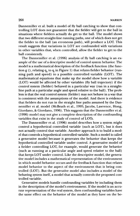
A model center fielder

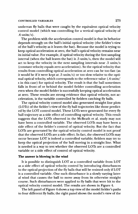
A generative model of fly ball catching behavior is shown in Figure 2.' The model represents a fielder playing straightaway center who catches fly balls by controlling optical velocity. This optical velocity control model was developed only to illustrate the concept of a controlled variable in the context of a generative model of behavior. Nevertheless, the results of this modeling effort suggest that more complex hypotheses about the controlled variable-optical acceleration and LOT-may not be necessary.

In the optical velocity control model, the fielder is modeled as two control systems. One system controls vertical optical velocity, qy,which is the time change in the vertical elevation of the ball relative to home plate. The other system controls lateral optical velocity, q,, which is the time change in the lateral position of the ball relative to the fielder's direction of gaze (the model fielder always looks straight ahead). In both

4 i

P ev P el

1 v iv0 010 i, 0 a0 Model Fielder

f, Environment

Figure 2. A generative model of fly ball catching behavior. The model is com- posed of two separate control systems: The system on the left controls vertical optical velocity; the system on the right controls lateral optical velocity

270 MARKEN

cases, the projection of the ball is onto a retinal plane that is normal to the fielder's direction of gaze.

The optical velocities, q, and q,, are environmental variables that are converted into one-dimensional perceptual signals, p,, and p,, by the input functions, iv() and 4 0 , respectively. These functions are linear, based on the assumption that the psychophysical function relating actual to perceptual velocity is linear, at least in the range of velocities experienced by a fielder. So pVis a time-varying signal that is proportional to qv, and p, is a time-varying signal that is proportional to q,. The input functions also add noise to each perceptual signal to simulate the fielder's imperfect sensitivity to differences in optical velocity. Low-pass filtered random noise was added to each perceptual signal; the average amplitude of the noise was approximately 2%of the average amplitude of each perceptual signal.

The reference signals in the model, rVand r,, represent the target values of pvand p,, respectively. Model behavior gave the best qualita- tive match to available fly ball catching data (ground running patterns and optical projections) when rVwas set to .0185, corresponding to an intention to see the vertical projection of the ball constantly rising at the rate of approximately .4 units/s, and r, was set at 0.0, indicating an intention to the see the lateral projection of the ball remain stationary. The model included a 100-ms transport lag to represent the time it takes for a perceptual signal originating at the retina to get to the point in the central nervous system where it is compared to the reference signal. So time-lagged versions of the perceptual signals, pVand p,, were continuously compared with the reference signals, q and 5.

The differences between the time-lagged perceptual signals and the reference signals in each system are the error signals, eV and q; eV is trans- formed, via the output function, oV(), into the forces that move the fielder forward or backward (depending on the sign of eV); q is trans- formed, via the output function o,(), into the forces that move the fielder leftward or rightward (depending on the sign of q). Output forces were limited to those that produce running speeds no greater than those that can be produced by a real fielder (a maximum of 6 m/s). The control system outputs move the fielder to different positions on the field (in a coordinate system where the x-axis is a line from home plate to straightaway center and the yaxis is perpendicular to the x-axis). The fielder's x position, fx, is determined by the forward or backward motions caused by the outputs of the system controlling vertical optical velocity, q,. The fielder's y position, fy , is determined by the leftward or rightward motions caused by the outputs of the system controlling lateral optical velocity, q,.

The fielder's position at any instant affects both controlled optical variables, qv and q,, via the laws of optics. These laws, which determine


how the fielder's position relates to the optical projection of the ball on the fielder's eye, are represented by the lines connecting system outputs to system inputs in Figure 2. The lines show that the fielder's x position, fx, affects both optical velocities, qv and q,, as does the fielder's y posi-tion, 4 . This means that movements in the x dimension that are aimed at control of qv are also a disturbance to q,; similarly, movements in the y dimension that are aimed at control of q, are also a disturbance to q,. This relationship between the fielder's inputs and outputs is the feedback function that connects the outputs of both control systems to the variables controlled by these systems.

Model behavior

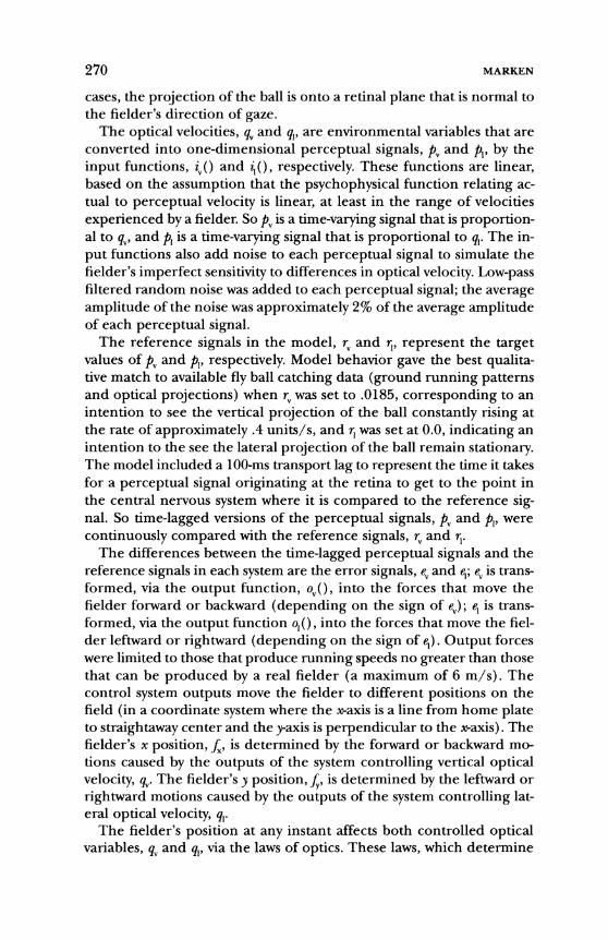
The model's ability to catch fly balls was tested by simulating fly balls hit in different trajectories relative to the model. The model started each catch from the same field position (defined by the initial values offx and A), which was located in straightaway center field, about 50 m from home plate. The balls were launched at a variety of realistic angles (vertical and lateral) and initial velocities (Adair, 1994). Vertical angles ranged from 42" to 48" from horizontal. Lateral angles ranged from +20° to -20" from the line connecting the fielder to home plate. Initial velocities off the bat ranged from 21 to 25 m/s. The trajectories were limited so that most balls could be caught, given the limits on the model fielder's output (running rate) capabilities.

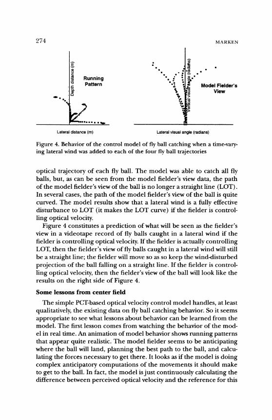
The behavior of the model as the fielder catches fly balls hit in four different trajectories is shown in Figure 3. The left panel shows a top view of the fielder's running path to the ball (changes in fx and f y over

(0 C m b Model Fielder's g 2 View

..

Y

Lateral distance (rn) Lateral visual angle (radians)

Figure 3. Behavior of the control model of fly ball catching. Data on the left are running paths to four different fly balls; data on the right are the optical projection of these four different fly balls as seen by the model

272 MARKEN

time). The right panel shows the model fielder's view of the ball during each fly ball trajectory.

The running paths on the left in Figure 3 are qualitatively similar to those observed for real fielders (see McBeath et al., 1995, Figure 3, p. 571; Jacobs et al., 1996, Figure 2A, p. 258). Like the real fielder, the model fielder moves laterally, in a curved path, before moving forward to intercept balls hit to the left or right of the fielder's starting position. The model fielder also shows an initial reverse movement for some trajectories that is also seen in some of the running patterns of the real fielder observed by McBeath et al. (1995). The exact shape of the model fielder's path to the ball depends on control system parameters, partic- ularly the relative gains of the systems controlling qv and q,, and the reference (2)for vertical velocity (the larger the value of rv,the less the model fielder backs up before running to the intercept point).

The model fielder's view of the fly ball trajectories on the right in Figure 3 are qualitatively similar to the fielder's view of the fly ball trajectories observed by McBeath et al. (1995, Figure 4, p. 572). The model fielder's views of the trajectories are basically LOTs, as are the fielder's views of such trajectories in the McBeath et al. (1995) data. These LOTs are a surprising side effect of controlling for optical velocity. The model fielder's views of the trajectories curve slightly away from a straight line, but careful inspection of the McBeath et al. data shows that the fielder's views of the trajectories curve in the same way. Again, the de- gree of curvature seen in the model's views of the trajectories depends on the model parameters, principally the relative gains of the systems controlling qv and q,. When these gains are high the model fielder's views of the trajectories have very little curvature; they are basically straight lines.

Comparing models

The optical velocity control model (Figure 2) is presented as an example of a model that generates behavior (running paths, model fielder's views of trajectories) that is qualitatively consistent with the available data on catching fly balls. The model is very similar to a model of fly ball catching developed by Tresilian (1995). The main difference between the models is the controlled variable, which in the present model is optical velocity and in Tresilian's model is optical acceleration. A comparison of equivalent versions of the models (equivalent in terms of running speed, gain, transport lag, and other relevant parameters) showed that the behavior of a model controlling optical velocity is not the same as the behavior of a model controlling optical acceleration. The comparison showed that the acceleration control model (which was controlling for a vertical optical acceleration of zero) often overran or


underran fly balls that were caught by the equivalent optical velocity control model (which was controlling for a vertical optical velocity of .4 units/s).

The problem with the acceleration control model is that its behavior depends strongly on the ball's initial optical velocity (the fielder's view of the ball's velocity as it leaves the bat). Because the model is trying to keep optical acceleration at zero, the ball's optical velocity remains near its initial value. For example, if optical velocity during the first sampling interval (when the ball leaves the bat) is .5 units/s, then the model will act to keep the velocity in the next sampling intervals near .5 units/s (constant velocity equals zero acceleration). So the optical velocity that results from controlling optical acceleration at zero can be too fast (as it would be if it were kept at .5 units/s) or too slow relative to the opti- mal optical velocity, which corresponds to the reference value (.4 units/ s in this case) for optical velocity. The result is that the ball sometimes falls in front of or behind the model fielder controlling acceleration even when the model fielder is successfully keeping optical acceleration at zero. These results are strong evidence that optical velocity, not acceleration, is the variable controlled by fielders catching fly balls.

The optical velocity control model also generated straight line plots (LOTs) of the fielder's view of the fly ball trajectories like those predict- ed by the LOT control model. These LOTs were generated for every fly ball trajectory as a side effect of controlling optical velocity. This result suggests that the LOTs observed in the McBeath et al. study may not have been a controlled variable. The observed LOTs may have been a side effect of the fielder's control of optical velocity. But the fact that LOTs are generated by the optical velocity control model is not proof that the observed LOTs are a side effect. In fact, the observed LOTs may occur because LOT is indeed a controlled variable; fielders may try to keep the optical projection of the ball moving in a straight line. What is needed is a way to test whether the observed LOTs are a controlled variable or a side effect of control of optical velocity.

The answer is blowing in the wind

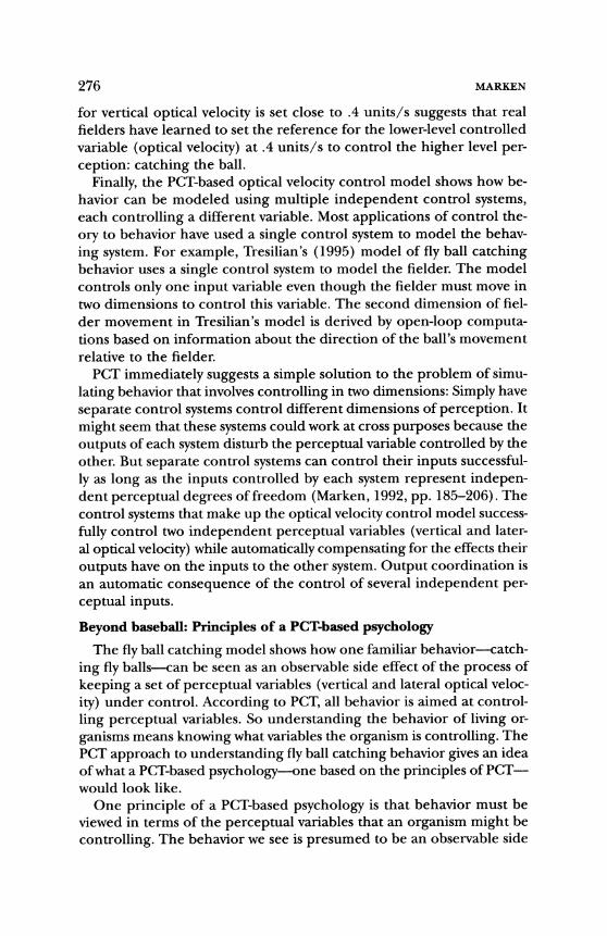
It is possible to distinguish LOT as a controlled variable from LOT as a side effect of optical velocity control by introducing disturbances to the optical projection of the fly balls that will be resisted only if LOT is a controlled variable. One such disturbance is a slowly varying lateral wind that causes the ball to move away from its otherwise straight course. Such disturbances were applied to fly balls that were hit to the optical velocity control model. The results are shown in Figure 4.

The left panel of Figure 4 shows a top view of the model fielder's paths to four different fly balls; the right panel shows the model's view of the

273 MARKEN

-E-

Running" Pattern. fam . n-...

........ Lateral distance (m) Lateral visual angle (radians)

Figure 4. Behavior of the control model of fly ball catching when a time-va~y- ing lateral wind was added to each of the four fly ball trajectories

optical trajectory of each fly ball. The model was able to catch all fly balls, but, as can be seen from the model fielder's view data, the path of the model fielder's view of the ball is no longer a straight line (LOT). In several cases, the path of the model fielder's view of the ball is quite curved. The model results show that a lateral wind is a fully effective disturbance to LOT (it makes the LOT curve) if the fielder is controlling optical velocity.

Figure 4 constitutes a prediction of what will be seen as the fielder's view in a videotape record of fly balls caught in a lateral wind if the fielder is controlling optical velocity. If the fielder is actually controlling LOT, then the fielder's view of fly balls caught in a lateral wind will still be a straight line; the fielder will move so as so keep the winddisturbed projection of the ball falling on a straight line. If the fielder is controlling optical velocity, then the fielder's view of the ball will look like the results on the right side of Figure 4.

Some lessons from center field

The simple PCT-based optical velocity control model handles, at least qualitatively, the existing data on fly ball catching behavior. So it seems appropriate to see what lessons about behavior can be learned from the model. The first lesson comes from watching the behavior of the model in real time. An animation of model behavior shows running patterns that appear quite realistic. The model fielder seems to be anticipating where the ball will land, planning the best path to the ball, and calculating the forces necessary to get there. It looks as if the model is doing complex anticipatory computations of the movements it should make to get to the ball. In fact, the model is just continuously calculating the difference between perceived optical velocity and the reference for this


velocity. The behavior of the optical velocity model suggests that the appearance of anticipation in purposive activities (Wing & Lederman, 1998) may be an illusion. The model shows the importance of identify- ing controlled variables and developing models that generate behavior by controlling these variables before concluding that any behavior is the result of anticipatory plans and calculations.

A second lesson from the model concerns reference states for controlled variables. An often unnoticed assumption that has been made since the earliest applications of control theory to human manual tracking behavior (McRuer & Krendel, 1959) is that the only possible reference state for controlled variables is zero. In studies of tracking this shows up as the assumption that any nonzero distance between the cursor and the target is an error. Of course, this is true only if the controller intends to keep the controlled variable-the distance between the cursor and the target-at zero. If the controller intends to keep the distance between cursor and target at some value other than zero (a nonzero reference state), then a nonzero distance between the cursor and the target is not an error. In fact, this nonzero distance is the distance that results in zero error.

The option of selecting a nonzero reference for the controlled variable is made explicit in PCT because the reference signal is shown in the diagram of the control system model of performance (see Figures 1 and 2). Control system diagrams that are not based on PCT typically leave out the reference signal (see, for example, Tresilian, 1995, Figure 1, p. 692), which seems to encourage the assumption that the control system is an input-output transfer function with a nominal offset (reference signal value) of zero. This is the assumption made by the OAC model of fly ball catching (Babler & Dannemiller, 1993; Tresilian, 1995). The OAC model keeps optical velocity nonzero when its reference for optical acceleration is set to zero. But the nonzero optical velocity produced by the OAC model is not always the one that gets the fielder to the ball. The PCT-based optical velocity control model is able to catch balls that are missed by the OAC model because it explicitly sets a specific nonzero reference for vertical optical velocity.

PCT assumes that reference signals are set by higher-level control systems in the organism itself; the nonzero reference for vertical optical velocity is presumably set by a higher-level system that is controlling some other perception, such as the perception of the ball being caught. This is hierarchical control (Powers, 1979). The higher-level systems in the hierarchy control perceptions by setting an appropriate (in this case nonzero) reference for the perceptions controlled by the lower-level systems (such as those controlling optical velocity). The fact that the optical velocity control model can catch the ball only when its reference

276 MARKEN

for vertical optical velocity is set close to .4 units/s suggests that real fielders have learned to set the reference for the lower-level controlled variable (optical velocity) at .4 units/s to control the higher level perception: catching the ball.

Finally, the PCT-based optical velocity control model shows how behavior can be modeled using multiple independent control systems, each controlling a different variable. Most applications of control theory to behavior have used a single control system to model the behaving system. For example, Tresilian's (1995) model of fly ball catching behavior uses a single control system to model the fielder. The model controls only one input variable even though the fielder must move in two dimensions to control this variable. The second dimension of fielder movement in Tresilian's model is derived by open-loop computations based on information about the direction of the ball's movement relative to the fielder.

PCT immediately suggests a simple solution to the problem of simulating behavior that involves controlling in two dimensions: Simply have separate control systems control different dimensions of perception. It might seem that these systems could work at cross purposes because the outputs of each system disturb the perceptual variable controlled by the other. But separate control systems can control their inputs successfully as long as the inputs controlled by each system represent independent perceptual degrees of freedom (Marken, 1992, pp. 185-206). The control systems that make up the optical velocity control model successfully control two independent perceptual variables (vertical and lateral optical velocity) while automatically compensating for the effects their outputs have on the inputs to the other system. Output coordination is an automatic consequence of the control of several independent perceptual inputs.

Beyond baseball: Principles of a PCT-based psychology

The fly ball catching model shows how one familiar behavior-catching fly balls-can be seen as an observable side effect of the process of keeping a set of perceptual variables (vertical and lateral optical velocity) under control. According to PCT, all behavior is aimed at controlling perceptual variables. So understanding the behavior of living organisms means knowing what variables the organism is controlling. The PCT approach to understanding fly ball catching behavior gives an idea of what a PCT-based psychology-one based on the principles of PCT- would look like.

One principle of a PCT-based psychology is that behavior must be viewed in terms of the perceptual variables that an organism might be controlling. The behavior we see is presumed to be an observable side


effect of the organism's efforts to keep controlled variables under control. This was the case in the fly ball catching studies, where it was assumed that the observed running patterns were a side of effect of the fielder's efforts to control an optical perception. An analogous situation exists for other observable behavior. For example, a PCT-based approach to understanding the observed egg-rolling behavior of the greylag goose (Lorenz, 1981) would be based on the assumption that the observed behavior is a side effect of the goose's efforts to control some perceptual variable, such as sensed pressure on the inside of the bill. Complex movements of the bill, such as those that occur when the egg is surrep- titiously removed, could then be understood as outputs aimed at protecting the pressure perception (the controlled variable) from disturbance.

A second principle of a PCT-based psychology is that evidence of controlled variables must come from studies in which individuals are tested one at a time, as in the fly ball catching research. Runkel (1990) called this research approach the method of specimens. It should be possible to find evidence of many types of controlled variables in existing psychological studies of behavior, even if these studies were not intentionally designed to expose the existence of controlled variables. But this is true only if these studies used the method of specimens. Stud- ies of the average behavior of groups of individuals cannot reveal what variables each individual is controlling unless all individuals happen to be controlling exactly the same variables. Indeed, the behavioral laws revealed by group averages can be precisely the opposite of the laws that actually characterize the behavior of the individuals in the group (Pow- ers, 1990).

One field of psychological research in which the method of specimens is common is the study of operant behavior. The goal of the study of operant behavior is ostensibly to discover the variables that control behavior. But it is possible to look at operant behavior from the perspective of PCT and see evidence of variables that are controlled by behavior (controlled variables). For example, studies of the effects of reinforcement schedules on behavior suggest that organisms vary their responding appropriately to keep rate of reinforcement constant (Stad- don, 1979). The rate at which reinforcements are received from the apparatus may be a variable that organisms control.

Another field of research in which the method of specimens is common is the study of cognitive processes. For example, Atwood and Pol- son (1976) studied problem solving by looking at the behavior of individual subjects solving water jar problems. Their research suggests that the relative amount of water in the jars is the controlled variable. The reference state for this variable seems to be the relative amounts of water

278 MARKEN

in the jars in the solution state of the problem. Evidence that people try to make the current problem state look as much as possible like the solution state comes from the fact that, given a choice between a legal move that makes the relative amounts of water look more like the solution state and one that makes the relative amounts look less like the solution state, a person nearly always chooses the former rather than the latter. Trying to achieve this reference state for the controlled variable makes problem solution difficult because to solve a waterjar problem the person must select some moves that make the relative amounts of water in the jars look less, rather than more, like the solution state.

A third principle of a PCT-based psychology is that evidence of controlled variables must come from studies in which individuals can control the possible controlled variable. In the fly ball catching studies, fielders were able to control all possible controlled variables because impossible trajectories (leading to fly balls that could not be caught) were not used. But possible controlled variables often are found to be uncontrollable in otherwise appropriate studies of purposeful behavior. For example, in many operant scheduling experiments, the organism has very little influence over possible controlled variables, such as the amount of reinforcement received. The typical operant schedule is ar- ranged so that the organism can get only a fraction of the reinforcement that it wants even when it is responding at its maximum rate. This means that it is impossible to tell whether any failure to keep a variable (such as reinforcement rate) at a particular level (reference state) occurs because the organism is not controlling the variable or because it cannot control the variable.

A fourth principle of a PCT-based psychology is that evidence of controlled variables must come from studies that use some version of the TCV to determine whether a particular variable is under control. The fly ball catching studies did use a version of the TCV in which possible controlled variables were monitored while disturbances (varying trajectories) were applied. Unfortunately, the steps involved in doing the TCV rarely are carried out in most psychological research studies. For example, the TCV is rarely applied in operant research. In particular, there is no monitoring of possible controlled variables while disturbances are applied.

It would be easy to replicate many operant experiments using the TCV. All that is needed is a way to produce disturbances while monitoring the state of possible controlled variables. A possible controlled variable such as reinforcement rate could be disturbed by delivering extra reinforcers after certain responses. Something like this was done by Teitelbaum (1966), who added extra food pellets randomly after certain lever presses in an operant situation. Although Teitelbaum did


not monitor the state of a hypothetical controlled variable while these disturbances occurred, the results suggest that organisms do adjust their response rates in a way that would keep some variable related to reinforcement rate under control.

Finally, a fifth principle of a PCT-based psychology is that the study of purposeful behavior must include the development of generative models that produce behavior by controlling the variables that are presumably being controlled by the real system. Generative models, such as Tresilian's (1995) model of fly ball catching behavior, make it possible to determine whether observed behaviors, such as the running patterns seen when fielders catch fly balls, would be produced by a system controlling the presumed controlled variables. Moreover, generative models make it possible to see whether the observed behaviors can be produced in an environment like that in which the real systems must behave.

Conclusion

This article has described an approach to understanding the purposeful behavior of living systems in terms of controlled variables. The approach, based on PCT, was illustrated in the context of studies aimed at determining how outfielders catch fly balls. The central feature of this approach is research aimed at discovering the variables organisms control when performing various purposeful behaviors. This research involves testing for controlled variables using the TCV and developing generative models that produce the behavior under study by controlling these variables. In the case of research on fly ball catching behavior, the TCV suggested three variables that fielders might be controlling when they run to intercept the ball: optical velocity, optical acceleration, and LOT. A generative model of fly ball catching suggests that the most likely controlled variable is optical velocity. The model also suggests a way to eliminate LOT as a possible controlled variable by looking for the effect of lateral wind disturbances on the optical path of the fly ball.

Once a controlled variable has been identified correctly, it is possible to understand many aspects of the behavior under study. The optical velocity control model (Figure 2) shows how correct identification of a controlled variable (optical velocity) makes it possible to understand many aspects of the behavior observed when fielders catch fly balls. The model also makes clear (and thus clearly falsifiable) predictions of other behaviors that should be observed (Figure 4) if fielders actually do control optical velocity.

According to PCT, all purposeful behavior involves controlling some perceptual aspect of the environment. This means that it should be

280 MARKEN

possible to explain all purposeful behavior in terms of controlled variables. To do this, it will be necessary to begin the search for controlled variables in earnest. The aim of this article is to encourage a systematic search for the controlled variables that underlie various purposeful behaviors. This search can be centered around any purposeful behavior. All that is needed is some evidence that these behaviors are purposeful; that there is an effort to produce a preselected state of some variable while protecting this variable from the effects of disturbance. Other aspects of these behaviors, such as learning and memory, can then be understood in terms of their relationship to the basic process of purposeful behavior: the control of perception (Powers, 1973a).

Notes

Correspondence about this article should be addressed to Richard S. Marken, 10459 Holman Avenue, Los Angeles, CA 90024 (e-mail: rmarkenaearthlink. net). Received for publication August 10, 1999; revision received December 14, 1999.

1. A Java simulation of the optical velocity control model is available on the World Wide Web at http://home.earthlink.net/-rmarken/ControlDemo/ CatchXY.htm1.

References

Adair, R. K. (1994). The physics of baseball. New York: HarperCollins. Atwood, R., & Polson, P. (1976). A process model of water jar problems. Cogni-

tive Psychology, 8, 191-216. Babler, T., & Dannemiller, J. (1993). Role of acceleration in judging landing

location of free-falling objects. Journal of Experimental Psychology: Human Perception and Performance, 19, 15-31.

Chapman, S. (1968). Catching a baseball. A m ' c a n Journal of Physics, 36, 868-870.

Dannemiller, J. L., Babler, T. G., & Babler, B. L. (1996). Technical comment. Science, 2 73, 256-257.

Dienes, Z . , & McLoed, P. (1993). How to catch a cricket ball. Perception, 22, 1427-1439.

Jacobs, T. M., Lawrence, M. D., Hong, K., Giordano, N., & Giordano, N. (1996). Technical comment: On catching fly balls. Science, 273, 257-258.

Lorenz, K. Z. (1981). The foundations ofethology. New York: Springer-Verlag. Marken, R. S. (1990). A science of purpose. American Behavioral Scientist, 34, 6-

13. Marken, R. S. (1992). Mind readings: Expa'mental studies ofpuqbose. Gravel Switch,

KY: CSG Publishing. Marken, R. S. (1993). The blind men and the elephant: Three perspectives on

the phenomenon of control. Closed Loop, 3( l ) , 37-46.

http://home.earthlink.net/-rmarken/ControlDemo/

CONTROLLED VARIABLES 281

Marken, R. S. (1997).The dancer and the dance: Methods in the study of living control systems. Psychological Methods, 2, 436-446.

McBeath, M. K., Shaffer,D. M., & Kaiser, M. K. (1995).How baseball outfielders determine where to run to catch fly balls. Science, 268, 569-573.

McBeath, M. K., Shaffer, D. M., & Kaiser, M. K. (1996).Technical comment: Response. Science, 273, 258-260.

McRuer, D. T., & Krendel, E. S. (1959).The human operator as a servo system element.Journal of the Franklin Institute, 267, 381-403.

Peper, L., Bootsma, R. J., Mastre, D. R., & Bakker, F. C. (1994).Catching balls: How to get the hand to the right place at the right time. Journal ofExpa'- mental Psychology: Human Perception and Perfmance, 20, 591-612.

Powers, W. T. (1973a). Behavior: The control of perception. New York: Aldine-De- Gruyter.

Powers, W. T. (1973b).Feedback: Beyond behaviorism. Science, 179, 351-356. Powers, W. T. (1978).Quantitative analysis of purposive systems: Some spade-

work at the foundations of scientific psychology. Psychological Review, 85, 417-435.

Powers, W. T. (1979).The nature of robots: Part 4. Looking for controlled variables. Byte, 4, 96112.

Powers, W. T. (1990). Control theory and statistical generalizations. American Behavioral Scientist, 34, 24-3 1.

Runkel, P. (1990). Casting nets and testing specimens. New York: Praeger. Staddon,J. E. R. (1979).Operant behavior as adaptation to constraint. Journal

of Experimental Psychology: General, 108, 48-67. Teitelbaum, P. (1966).The use of operant methods in the assessment and con-

trol of motivational states. In W. K. Honig (Ed.),Operant behavior. NewYork: Appleton-Century-Crofts.

Tresilian,J. R. (1995).Study of a servocontrol strategy for projectile intercep- tion. Quarterly Journal of Expm'mental Psychology, 48A, 688-715.

Watson,J . B. (1913).Psychology as the behaviorist views it. Psychological Review, 20, 158-177.

Wing, A. M., & Lederman, S. J. (1998).Anticipating load torques produced by voluntary movements. Journal ofExpaimenta1 Psychology: Human Perception and Performance, 24, 1571-1581.

Controlled Variables: Psychology as the Center...

Documents

Transcript of Controlled Variables: Psychology as the Center...