PDF - 4.1 MB

3.012 Fundamentals of Materials Science Fall 2005

Lecture 23: 12.05.05 Lattice Models of Materials; Modeling Polymer Solutions

Today:

LAST TIME .........................................................................................................................................................................................2The Boltzmann Factor and Partition Function: systems at constant temperature..................................................................2A better model: The Debye solid.................................................................................................................................................3

EXAMINATION OF HEAT CAPACITIES OF DIFFERENT MATERIALS ....................................................................................................6DEGREES OF FREEDOM IN MOLECULAR MODELS(1) ........................................................................................................................8

Excitations in materials ...............................................................................................................................................................8Complete molecular partition functions.....................................................................................................................................9

LATTICE MODELS FOR TRANSLATIONAL DEGREES OF FREEDOM ..................................................................................................11Assumptions in simple lattice models .......................................................................................................................................11

FLORY-HUGGINS THEORY OF POLYMER SOLUTIONS ...................................................................................................................13The entropy of polymer solutions..............................................................................................................................................13

REFERENCES ...................................................................................................................................................................................19

Reading: Engel and Reid 32.3-32.4

Dill and Bromberg Ch. 15 ‘Solutions & Mixtures,’ pp. 267-273

Dill and Bromberg Ch. 31 ‘Polymer Solutions,’ pp. 593-605.

Supplementary Reading: Details of rotational, vibrational, and electronic partition functions for simple molecules: Engel and Reid 32.5-32-9

Lecture 24 – Lattice Models of Materials 1 of 1912/5/05


Last time

The Boltzmann Factor and Partition Function: systems at constant temperature

How do we treat systems at constant temperature in statistical mechanics? We needed to determine how the probability of model microstates depends on temperature. We found the answer by minimizing the Helmholtz free energy with respect to the possible microstate probabilities pj. This analysis gave us the Boltzmann factor and the partition function:

Once we had the concept of the partition function, we began tackling a first example problem: the Einstein solid. Atoms of a crystalline solid are assumed to vibrate in x, y, and z with a single well-defined frequency as quantum mechanical harmonic oscillators. We started by solving for the molecular partition function:

From here we determined the partition function for a system of N non-interacting, identical, distinguishable oscillators:

!

Q =e

"h#

2

e"h# $1

%

&

' ' '

(

)

* * *

3N

=e

h#

2kT

e

h#

kT $1

%

&

' ' '

(

)

* * *

3N

The partition function for this simple model allowed calculations of the internal energy and heat capacity of a crystalline solid:

!

CV

= 3Nkb

"E

T

#

$ %

&

' (

2

e

"E

T

e

"E

T )1#

$ %

&

' (

2

Lecture 24 – Lattice Models of Materials 2 of 19 12/5/05


Figure by MIT OCW.

A better model: The Debye solid

The Einstein model makes the simplification of assuming the atoms of the solid vibrate at a single, unique frequency:

g g

v v t

(a) (b)

Frequency distribution g(v) for crystal. (a) Einstein approximation. (b) Debye approximation.

vml

Figure by MIT OCW.

Den

sity

of s

tate

s g(w

)

0 1 2 3 4 5

�D

�/1013 radians s-1

The Debye distribution of frequencies, with the experimental distribution of frequencies

function of � = 2�is obviously complicated enough that a theory to reproduce such a distribution would likely

for copper. The distribution is shown as a v. The experimental distribution

be difficult to produce.

Figure by MIT OCW.

‘g’ in Figure 5-4 above from Hill is the distribution of vibrational frequencies present in the crystal. In the Einstein model, only one vibrational frequency is assumed for all atoms in the crystal. However, atoms sitting on different lattice sites may have difference accessible vibrational frequencies- which depend on what neighbors they ‘feel’ around them- this is seen in the complex distribution of vibrational frequencies shown in Figure 22.8 from Mortimer for a real sample of copper. The Debye model approximates the true frequency distribution by assuming the distribution shown in Figure 5-4(b): a distribution that is continuous up to some frequency cut-off (νm). The Debye expression for heat capacity becomes:



EINSTEIN MODEL DEBYE MODEL

!

CV

= 3Nkb

"E

T

#

$ %

&

' (

2

e

"E

T

e

"E

T )1#

$ %

&

' (

2

!

CV = kb

h"

kbT

#

$ %

&

' (

2

e

h"

kbT

e

h"

kT )1#

$ %

&

' (

2g "( )d"

0

*

+

This approximation leads to a heat capacity behavior near zero Kelvin which better captures experimentally-observed behavior:

!

T" 0, CV"

12Nkb# 4

5

T

$D

%

& '

(

) *

3

where $D +h,

m

kb

%

& '

(

) * = Debye temperature

The Debye model performs quite well for predicting the thermal behavior of many solid materials:

Debye Einstein Al �D = 385 K

25

20

15

10

5

0 0 .4 .8 1.2 1.6 2.0

. mol

e

T/�

Comparison among the Debye heat capacity, the Einstein heat capacity, and the actual heat capacity of aluminum.

Cv,

joul

es/d

egre

e

Figure by MIT OCW.



Examination of heat capacities of different materials

• If heat capacities correlate with molecular degrees of freedom in a material, we might expect materials that have similar degrees of freedom to have similar heat capacities. This is in fact seen for many materials. Consider first a comparison of the heat capacity in 3 different crystalline non-metals:2

Cp, J/ mol.K

90

80

70

60

50

40

30

20

10

0 0 50 100 150 200 250 300 350

Temperature, K

Molar heat capacity at constant pressure of three crystalline nonmetals.

NiSe2 9R

6RNaCl

Ge 3R

Figure by MIT OCW.

(Ge crystal structure from www.webelements.com)

o Thus in these structurally-related crystals, the heat capacity per NAv atoms is very similar, ~3R, or 25 J/mole K. We will show later in the term that this plateau value can be predicted by treating the atoms in the solid as a collection of harmonic oscillators.



cv /3R

1.0

0.8

0.6

0.4

0.2

0

Rbl NaCl FeS2 MgO

Diamond

0 100 200 300 400 500 600 700 800 900 1000 Temperature, K

Temperature variation of cv /3R of nonmetals. (1 mol of diamond, 1mol of Rbl, NaCl,21and MgO; and 3

mol of FeS2.)

Figure by MIT OCW.



Degrees of freedom in molecular models(1)

Excitations in materials

• We modeled the atomic vibrations in a crystalline solid using 3 degrees of freedom- harmonic oscillations in X, Y, and Z. We saw that a model using only these 3 degrees of freedom provides reasonable predictions for the behavior of the heat capacity of many solids. Other materials may have other important degrees of freedom that we should account for to obtain good statistical mechanics predictions of their behavior. The important molecular degrees of freedom include:

1. Translation 2. Rotation 3. Vibration 4. Electron excitation

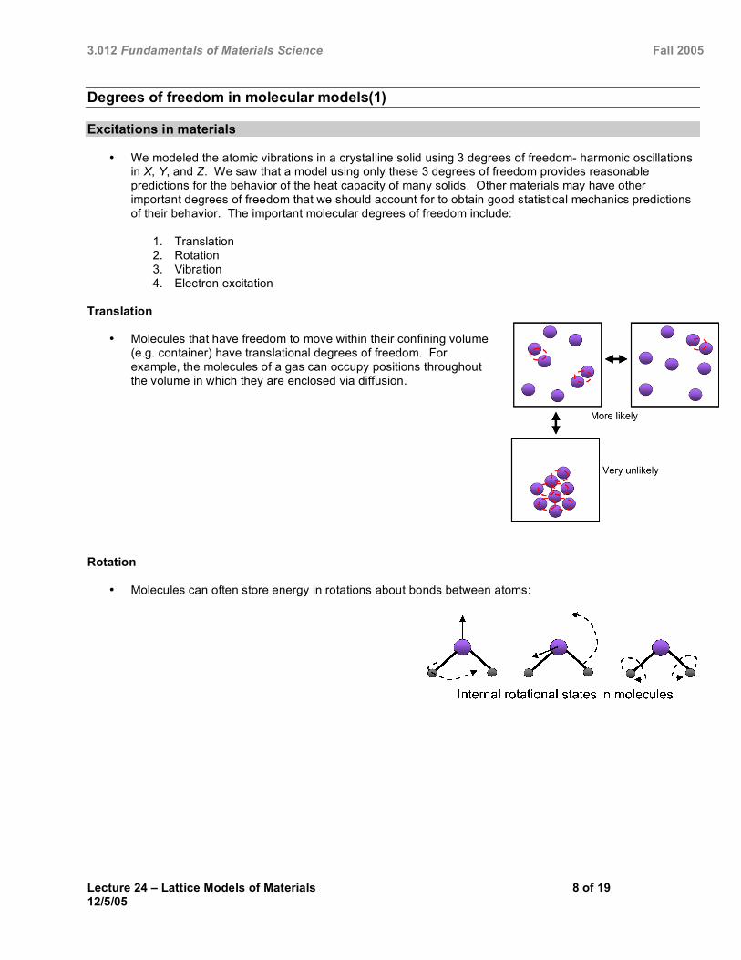
Translation

• Molecules that have freedom to move within their confining volume (e.g. container) have translational degrees of freedom. Forexample, the molecules of a gas can occupy positions throughoutthe volume in which they are enclosed via diffusion.

Rotation

• Molecules can often store energy in rotations about bonds between atoms:



Vibration

• The electronic glue holding molecules together allows vibrations that store energy:

Electronic excitations Figure by MIT OCW.

Symmetric stretch

Symmetric stretch

Bend

Bend

Asymmetric strech

Asymmetric strech

V1 = 1340 cm2

V12

V2 = 007 cm2

V2 = 519 cm2

V3 = 2340 cm2

V3 = 1361 cm2

Vibrational modes of carbon dioxide.

= 1151.2 cm

0 -82

-146

-328

-1313

0 -82

-146

-328

-1313 1s

1s

4s

4s

2s

2s

3s

3s

4p 4p

3p 3p

2p 2p

4d 4d

3d 3d

4f 4f

Hydrogen Multielectron atoms

Orb

ital E

nerg

y (k

J / m

ol)

Figure by MIT OCW.

Complete molecular partition functions

• A complex system may have all of these degrees of freedom. To make calculations for a given model, we need to know how to put these degrees of freedom together in the partition function.

Independent degrees of freedom

A common approximation is to assume that each degree of freedom in the molecules of the system is independent, with a unique amount of energy for each possible state of that degree of freedom (let’s use DOF as an abbreviation for degree of freedom). Thus a molecule with both vibrational and electronic DOFs has states characterized by one total energy containing independent contributions from the vibration and electronic excitations:



o The subscript j refers to the single state that has the given characteristic vibrational and electronic energy. Because we assume they are independent, the value of Ej

vib does not depend on the value of Ej

elec, and vice versa. The partition function of this system with independent DOFs is:

Where the independent energies have been split off into partition functions for each DOF, qvib and qelec.

o In general, a complete molecular partition function made up of independent degrees of freedom can be written as the product of the individual DOF partition functions:



Lattice models for translational degrees of freedom

• We introduced statistical mechanics as a set of tools for calculating macroscopic thermodynamic quantities from molecular models. These models can be derived either from quantum mechanics (e.g. the Einstein solid) or from simpler non-quantum models. There are many cases when the quantum nature of available energies in the system of interest do not dominate and we can use so-called ‘coarse-grained’ lattice models to capture the important aspects of the material’s behavior.

o Earlier, we have seen that chemical potential models such as the regular solution or ideal solution mimic some real experimental data reasonably well. However, a question unanswered is- where did this model come from? What about the regular solution model- how do molecular interactions give rise to miscibility gaps? Answers to these questions can be found in simple lattice models.

Assumptions in simple lattice models

ASSUME:

Figure by MIT OCW.



In this simple lattice model, we assume that only translational degrees of freedom matter in the determination of possible statistical mechanical states- the states of the system are simply defined by the number of unique ways the molecules can be arranged on the lattice. We take N for the total number of molecules (N = NA + NB). To determine the entropy of mixing, we need the number of distinguishable states W for the mixed and unmixed components. For the unmixed pure components, there is only one distinguishable state (all lattice sites occupied by either A or B), so the entropy is 0 (S = k ln 1 = 0).

These assumptions can be used to derive both the ideal solution model of the chemical potential and the regular solution chemical potential.

As an example of the utility of lattice models for materials, we will now derive the entropy and enthalpy of mixing using a simple lattice model for polymer solutions, based on the Flory-Huggins theory of polymer solutions.

o Paul J. Flory’s extensive work on the statistical thermodynamics of polymers was awarded the nobel prize in chemistry in 1974

Image removed for copyright reasons. Photograph of P. J. Flory.




Flory-Huggins Theory of Polymer Solutions

• Flory-Huggins theory was developed to provide a molecular theoretical basis for the free energy behavior of polymer solutions- to allow predictions of miscibility behavior based on polymer molecular structure. Thus, our objective is to derive a theoretical description of the free energy of mixing, which can be used to predict phase diagrams of polymer solutions:

!

"Gmix

= "Hmix#T"S

mix= ?

The entropy of polymer solutions

To model a polymer solution- a collection of high molecular weight polymer chains mixed with a small-molecule solvent, we model the polymer chains as beads connected by unbreakable bonds on a cubic lattice. Solvent molecules fill single sites of the 3D lattice:

volume fraction of polymer:

!

"p =Vp

Vp +Vs

=Nnp

M

volume fraction of solvent:

!

"s =Vs

Vp +Vs

=ns

M

Unmixed State Mixed StatePure Polymer Pure Solvent (Homogeneous Solution)

+

Figure by MIT OCW.


In this lattice model, we are concerned with one degree of freedom in the calculation of the entropy- the translational entropy:

!

"Smix = Ssolution # Sunmixed = Ssolution # S

pure polymer + Spure solvent( )

We are thus looking to derive expressions for Wsolution and Wpure polymer- the number of configurations possible for the polymer + solvent or the polymer alone on a 3D lattice.

CONFIGURATIONS OF A SINGLE CHAIN

We start by looking at the number of ways to place a single polymer chain on the lattice:

o What are the number of conformations for first bead?

o With the first bead placed on the lattice, what is the number of possible locations for the second segment of the chain?



o Moving on to placement of the third segment of the chain:

o We repeat this process to place all N segments of the chain on the lattice, and arrive at ν1, the total number of configurations for a single chain:

COUNTING CONFIGURATIONS FOR A COLLECTION OF CHAINS

o We can follow the same procedure shown above for a single chain to obtain the number of configurations possible for an entire set of np chains. We start by placing the FIRST SEGMENT OF ALL np CHAINS. The number of configurations for the first segment of all np chains is ν first:

o The number of configurations for the (N - 1) remaining segments of all np chains is ν subsequent:




o Putting these two configuration counts together, we have the total number of configurations for

the collection of np chains of N segments each:

!

W =" first" subsequent

np!

The factor of np! Corrects for the

over-counting since the polymer chains are indistinguishable, and we can’t tell the difference between two configurations with the same polymer distributions but different chain identities:

We are now ready to calculate the number of unique states for the unmixed and mixed states:

o UNMIXED STATE: PURE SOLVENT:

PURE POLYMER:

Nnp = M

Wpure polymer =z "1

M

#

$ %

&

' (

n p (N"1)M!

M " Nnp( )!np!

Spure polymer = kb lnWpure polymer

Figure by MIT OCW.

Figure by MIT OCW.


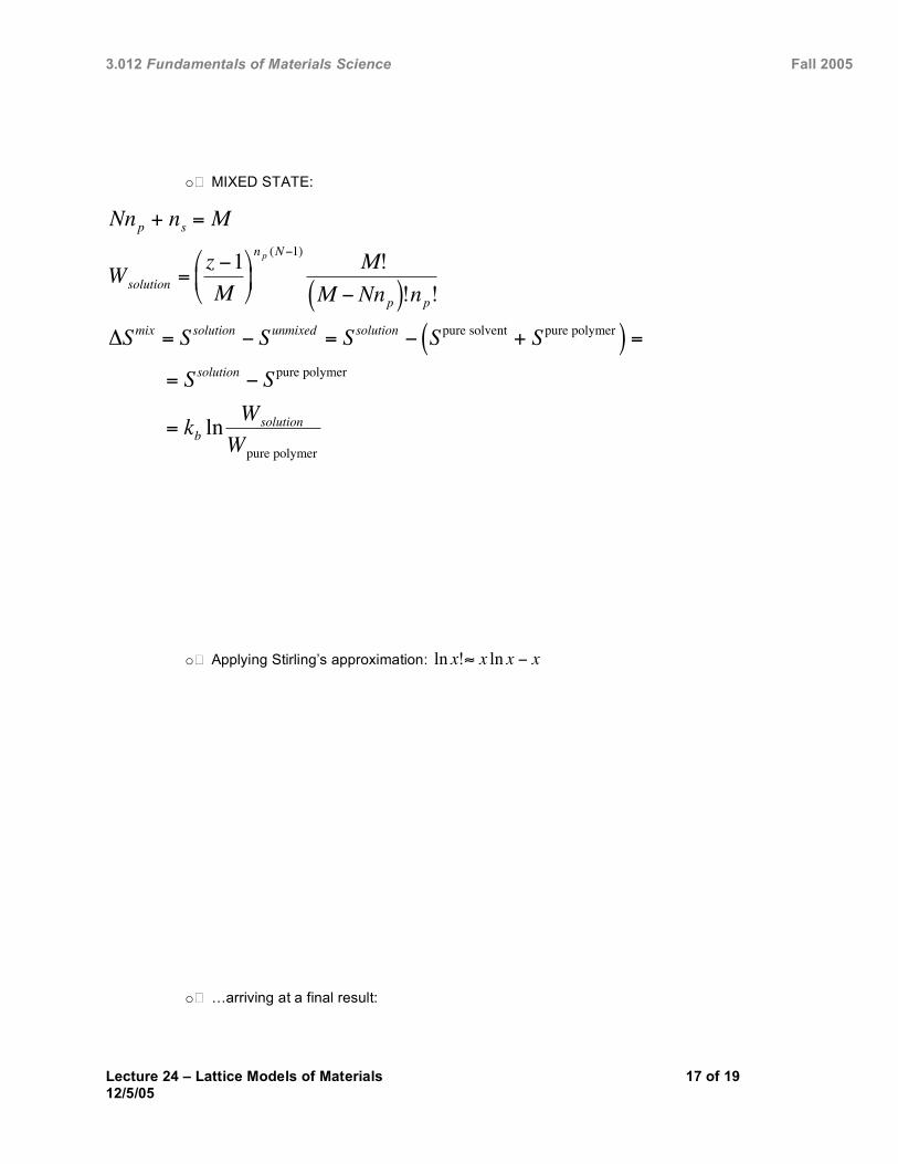
o MIXED STATE:

!

Nnp + ns = M

Wsolution =z "1

M

#

$ %

&

' (

n p (N"1)M!

M " Nnp( )!np!

)Smix = Ssolution " Sunmixed = Ssolution " Spure solvent + Spure polymer( ) =

= Ssolution " Spure polymer

= kb lnWsolution

Wpure polymer

o Applying Stirling’s approximation:

!

ln x!" x ln x # x

o …arriving at a final result:



!

"#Smix = $kb ns ln%s + np ln%p[ ]

Lecture 24 – Lattice Models of Materials 18 of 1912/5/05


References

1. Dill, K., and S. Bromberg. 2003. Molecular Driving Forces, New York. 2. Mortimer, R. G. 2000. Physical Chemistry. Academic Press, New York. 3. .


PDF - 4.1 MB

Documents

Transcript of PDF - 4.1 MB