Paulo Maiocoller.tau.ac.il/.../management/seminars/account2/2015/cond0116.pdf · New evidence on...
63
New evidence on conditional factor models Paulo Maio 1 This version: January 2016 2 1 Hanken School of Economics, Department of Finance and Statistics. E-mail: paulof- [email protected] 2 I thank Frederico Belo for helpful comments. I am grateful to Kenneth French, Robert Shiller, and Lu Zhang for providing stock market data. Any remaining errors are mine.
Transcript of Paulo Maiocoller.tau.ac.il/.../management/seminars/account2/2015/cond0116.pdf · New evidence on...
New evidence on conditional factor models
Paulo Maio1
This version: January 20162
1Hanken School of Economics, Department of Finance and Statistics. E-mail: [email protected]
2I thank Frederico Belo for helpful comments. I am grateful to Kenneth French, Robert Shiller,and Lu Zhang for providing stock market data. Any remaining errors are mine.

Abstract
I estimate conditional multifactor models over a large cross-section of stock returns associated
with 25 CAPM anomalies. The four-factor model of Hou, Xue, and Zhang (2015a, 2015b)
clearly outperforms the competing models in pricing the extreme portfolio deciles and the
cross-sectional dispersion in equity risk premia. Yet, the five-factor model of Fama and
French (2015, 2016) outperforms in pricing the intermediate deciles. Therefore, the asset
pricing implications of the different versions of the investment and profitability factors are
quite different for a large cross-section of stock returns. The HML factor is largely redundant
within the five-factor model when using conditioning information.
Keywords: asset pricing models; conditional factor models; conditional CAPM; equity
risk factors; investment and profitability risk factors; stock market anomalies; cross-section
of stock returns; time-varying betas; HML
JEL classification: G10; G12

1 Introduction
Explaining cross-sectional equity risk premia represents one of the major goals in asset
pricing. Recently, this line of research has been particularly active with the emergence of new
multifactor models with the objective of representing the new work horses in the empirical
asset pricing literature. These include the four-factor model of Hou, Xue, and Zhang (2015b)
and the five-factor model of Fama and French (2015), which represent a response to the failure
of the traditional multifactor models (e.g., three-factor model of Fama and French (1993)
and four-factor model of Carhart (1997)) in explaining several market anomalies. The key
risk factors in both models are related with the investment and profitability anomalies, yet,
as shown in Hou, Xue, and Zhang (2015a) and Maio (2015), the performance of the two
models varies widely when it comes to price a large cross-section of stock returns.
This paper contributes to the empirical asset pricing literature by testing conditional
versions of the multifactor models mentioned above. In fact, a large body of the asset
pricing literature has focused on estimating conditional factor models in an attempt to
solve the failure of the baseline CAPM from Sharpe (1964) and Lintner (1965) when it
comes to explain several patterns in the cross-section of stock returns like the size, value,
and momentum anomalies. A partial list includes Ferson, Kandel, and Stambaugh (1987),
Harvey (1989), Cochrane (1996), He, Kan, Ng, and Zhang (1996), Jagannathan and Wang
(1996), Ferson and Harvey (1999), Lettau and Ludvigson (2001), Wang (2003), Petkova and
Zhang (2005), Avramov and Chordia (2006), Ferson, Sarkissian, and Simin (2008), and Maio
(2013). Yet, most of this literature focuses on the conditional CAPM and neglects the role
of conditioning information for multifactor models (with He, Kan, Ng, and Zhang (1996),
Ferson and Harvey (1999), Wang (2003), and Maio (2013) representing notable exceptions).
Following Hou, Xue, and Zhang (2015a, 2015b), I test conditional factor models over a
large cross-section of stock returns associated with 25 different CAPM anomalies. These
anomalies can be broadly classified in strategies related with value, momentum, investment,
profitability, and intangibles. In the benchmark test, the portfolios are value-weighted and all
1
the groups include decile portfolios, except “industry momentum” and “number of quarters
with earnings increases” with nine portfolios each. Following the conditional CAPM litera-
ture, I use four conditioning variables in the construction of the scaled risk factors—the term
spread, default spread, log dividend yield, and the one-month T-bill rate. In line with the
related literature, I employ the time-series regression approach to evaluate the alternative
factor models.
By conducting Wald tests on the joint significance of the scaled factors associated with
each of the original factors, it follows that the factor loadings are time-varying in most cases,
and thus, it makes sense to conduct conditional tests to evaluate the alternative multifactor
models. The analysis of the alphas for the 25 “high-minus-low” spreads in returns suggests
that using conditioning information has a relevant impact on the performance of the factor
models. The model that registers the greatest improvement relative to the unconditional
test is the five-factor model of Fama and French (2015, 2016) (FF5 henceforth), although
the four-factor model of Hou, Xue, and Zhang (2015a, 2015b) (HXZ4) shows the best overall
performance, similarly to the unconditional tests. Specifically, the four-factor model produces
a mean absolute alpha of 0.19% among the 25 spreads, compared to 0.28% for FF5 and 0.29%
for the four-factor model of Carhart (1997) (C4). There are seven (out of 25) statistically
significant alphas for HXZ4, compared to 12 for FF5 and 13 for C4.
When one tests the alternative models over the full cross-section of stock returns (for
a total of 248 portfolios), it turns out that the three models register a similar average
mispricing. Specifically, the root mean squared alpha is the same across C4, HXZ4, and FF5
(0.13%), whereas the mean absolute alpha estimates are 0.09% for FF5 compared to 0.10%
for both C4 and HXZ4. Yet, both HXZ4 and FF5 have a much lower number of individual
significant alphas than C4 (around 33 versus 51 for C4). The fact that FF5 produces an
average mispricing that is similar to that of HXZ4 stems from the former model doing better
in pricing the middle deciles, while HXZ4 clearly dominates when it comes to price the
extreme deciles. Moreover, this pattern is robust across the different classes of anomalies.
2

Across categories, it turns out that the three-factor model of Fama and French (1993)
(FF3), C4, and FF5 clearly dominate the HXZ4 model in terms of pricing the value anoma-
lies. On the other hand, both C4 and HXZ4 significantly outperform FF5 when it comes
to price the momentum-based anomalies, while HXZ4 is the clear winner in the group of
profitability anomalies. In the group of 11 investment-based anomalies, FF5 produces an
average alpha of 0.11% compared to 0.12% for both C4 and HXZ4. Yet, the number of
deciles with significant alphas in HXZ4 and FF5 (around 15) is slightly lower than for C4
(22). In the estimation within the intangibles category, we observe a similar performance for
both HXZ4 and FF5. By conducting a decomposition of equity risk premia for nine of the
most important individual anomalies (those with spreads above 0.50% in magnitude), one
observes that the most relevant conditioning variables in driving the fit of both HXZ4 and
FF5 are the TERM spread and the T-bill rate. Thus, both the dividend yield, and especially
the default spread, seem to play a less relevant role in pricing these nine spreads in returns.
I repeat the asset pricing tests by using equal-weighted portfolios, following previous ev-
idence that small stocks represent the major challenge for asset pricing models (e.g., Fama
and French (2012, 2015)). The results indicate that all factor models, and especially HXZ4,
have greater difficulty in pricing the equal-weighted portfolios than the value-weighted port-
folios. Yet, HXZ4 continues to beat the alternative models when it comes to price the spreads
high-minus-low, with a mean absolute alpha (across the 25 spreads) of 0.27%, compared to
0.37% for FF5 and 0.39% for C4. In contrast, the five-factor model produces the best fit in
the estimation with all 248 portfolios. Specifically, the root mean squared alpha is 0.16% for
FF5 compared to 0.16% and 0.17% for C4 and HXZ4, respectively, while the mean absolute
alpha estimates are 0.12%, 0.13%, and 0.15% for FF5, C4, and HXZ4, respectively. However,
FF5 produces a smaller number of significant alphas than the other models by a great margin
(62 compared to 102 and 125 for HXZ4 and C4, respectively). This shows that, similarly to
the benchmark test based on value-weighted portfolios, HXZ4 does a better job in pricing
the extreme deciles, while FF5 outperforms when it comes to explaining the intermediate
3

deciles.
I estimate a conditional restricted version of FF5 that excludes the HML factor. The
results show that in most cases the restricted model is not dominated by FF5. Specifically,
the mean absolute alpha across the 25 value-weighted spreads is 0.28% (the same as for
FF5). The average alpha across the 248 portfolios is 0.12% (compared to 0.13% for FF5),
and the model produces 30 significant alphas (compared to 34 for FF5). In the estimation
containing all 248 equal-weighted portfolios, the model that excludes HML produces an
average mispricing of 0.15%, versus 0.16% for FF5. These results largely confirm the previous
evidence for unconditional asset pricing tests (e.g., Fama and French (2015, 2016), Hou, Xue,
and Zhang (2015a)) that HML is redundant when in the presence of the investment and
profitability factors.
Following Maio (2015), I compute a cross-sectional R2 metric to evaluate the cross-
sectional dispersion in equity risk premia based on all portfolios, and not just the spreads
high-minus-low. This metric is based on the constraint that the factor risk price estimates are
equal to the corresponding factor sample means. The results confirm that the HXZ4 model
outperforms the competing models in terms of explaining the cross-sectional dispersion in
equity risk premia for a large number of anomalies, and these results hold for both value- and
equal-weighted portfolios. Specifically, in the estimation with 248 value-weighted portfolios
the R2 estimates are 53% for HXZ4, compared to 35% for both C4 and FF5. In the estimation
with all equal-weighted portfolios, the fit of HXZ4 is 69% versus 45% and 46% for C4 and
FF5, respectively.
Overall, the results of this paper show that the HXZ4 model outperforms the competing
models when it comes to price the extreme portfolio deciles and the cross-sectional dispersion
in equity risk premia. Yet, the FF5 model performs slightly better in terms of pricing the
intermediate deciles. This suggests, that even after accounting for the role of conditioning
information, the asset pricing implications of the different versions of the investment and
profitability factors are quite different for a large cross-section of stock returns. Moreover,
4

the HML factor continues to be largely redundant within the five-factor model when using
conditioning information.
The paper proceeds as follows. Section 2 shows the theoretical background, while Section
3 describes the data and methodology. The main empirical analysis is presented in Section
4. Section 5 shows the empirical results for equal-weighted portfolios, while in Section 6,
I analyze further the cross-sectional dispersion in equity risk premia. Finally, Section 7
concludes.
2 Conditional factor models
In this section, I present the theoretical background and the conditional factor models esti-
mated in the following sections.
2.1 Theoretical background
Consider the usual asset pricing equation in conditional form,
0 = Et(Mt+1Rei,t+1), (1)
where Rei,t+1 denotes the excess return on an arbitrary risky asset i and Mt+1 is the stochastic
discount factor (SDF).
Following Cochrane (1996, 2005) and Lettau and Ludvigson (2001), I define an SDF that
is linear on K original factors (fj,t+1), but with coefficients that are linear functions of a
5

predetermined instrument with zero mean (zt):1
Mt+1 = at +K∑j=1
bj,tfj,t+1, (2)
at = a0 + a1zt, (3)
bj,t = bj,0 + bj,1zt, j = 1, ..., K. (4)
In this specification, I am using a single instrument to simplify the algebra presented be-
low, but the analysis can be generalized in a straightforward way to the case of multiple
conditioning variables.
By applying the law of total expectations, we obtain the unconditional pricing equation,
0 = E(Mt+1Rei,t+1), (5)
which can be defined in expected return-covariance representation as
E(Rei,t+1) = −
Cov(Rei,t+1,Mt+1)
E(Mt+1). (6)
By substituting the expression for the SDF in the expected return-covariance equation
above, we obtain the SDF as a function of the instrument and the scaled factors (fj,t+1zt):
Mt+1 = a0 + a1zt +K∑j=1
bj,0fj,t+1 +K∑j=1
bj,1fj,t+1zt. (7)
The scaled factor is often interpreted as the return on a “managed portfolio” (see Hansen and
Richard (1987), Cochrane (1996, 2005), Bekaert and Liu (2004), and Brandt and Santa-Clara
1In a conditional pricing equation, even if one specifies an SDF with fixed coefficients it follows thatby forcing the model to price an arbitrary set of test assets (e.g., its factors if they represent returns) thecoefficients will be a function of conditional moments of the testing returns (and thus, will be time-varying).Cochrane (2005) (Chapter 8) provides a simple example with the CAPM, in which the model is forced to pricethe market return and the risk-free rate. This originates SDF coefficients that depend on the conditionalmean and variance of the market return and also on the time-varying risk-free rate.
6
(2006)).
It can be shown that, by substituting the new expression of the SDF into the expected
return-covariance equation, one obtains the following multifactor model in expected return-
beta form,2
E(Rei,t+1) =
K∑j=1
βi,jλj +K∑j=1
βi,jzλjz, (8)
where the factor loadings are obtained from the following time-series regression:
Rei,t+1 = αi +
K∑j=1
βi,jfj,t+1 +K∑j=1
βi,jzfj,t+1zt + εi,t+1. (9)
This regression is equivalent to a conditional specification in which the loadings on the
original factors are allowed to be time-varying and affine in the instrument:
Rei,t+1 = αi +
K∑j=1
(βi,j + βi,jzzt)fj,t+1 + εi,t+1. (10)
Thus, a K-factor conditional model is equivalent to a 2K-factor model in the equivalent
unconditional representation.3 Moreover, specifying a SDF with time-varying coefficients is
equivalent to modelling a beta representation with time-varying factor loadings.
As noted in Cochrane (2005) and Maio (2015), when the factors represent excess returns,
the risk prices are restricted to be equal to the corresponding factor means,
E(fj,t+1) = λj, (11)
E(fj,t+1zt) = λjz, j = 1, ..., K. (12)
These conditions are obtained by applying the beta equation above for each factor, and
noting that each factor has a (multiple regression) beta of one on itself and a beta of zero
2The full derivation is available upon request.3I follow most of the literature on the conditional CAPM by estimating the unconditional representation
of the conditional factor models. Nagel and Singleton (2011) and Ang and Kristensen (2012) use alternativemethods to estimate the conditional CAPM.
7
on all the other factors.4 By substituting the restrictions on the factor risk prices back into
the beta equation, we obtain the following multifactor model:
E(Rei,t+1) =
K∑j=1
βi,j E(fj,t+1) +K∑j=1
βi,jz E(fj,t+1zt). (13)
This specification represents the basis for the empirical work conducted in the following
sections.
2.2 Models
Next, I present the conditional factor models tested on the cross-section of stock returns.
The first model analyzed is the conditional CAPM,
E(Rei,t+1) = E(RMt+1)βi,M + E(RMt+1zt)βi,Mz, (14)
where RM denotes the excess market return.
The second model is a conditional version of the Fama and French (1993, 1996) three-
factor model (henceforth FF3),
E(Rei,t+1) = E(RMt+1)βi,M + E(RMt+1zt)βi,Mz + E(SMBt+1)βi,SMB + E(SMBt+1zt)βi,SMBz
+ E(HMLt+1)βi,HML + E(HMLt+1zt)βi,HMLz, (15)
where SMB and HML represent the size and value factors, respectively.
The third model analyzed is the conditional four-factor model from Carhart (1997) (C4,
4This restriction also applies to the scaled factors since they represent the returns on traded assets.
8

henceforth), which adds a momentum factor (UMD) to FF3:
E(Rei,t+1) = E(RMt+1)βi,M + E(RMt+1zt)βi,Mz + E(SMBt+1)βi,SMB + E(SMBt+1zt)βi,SMBz
+ E(HMLt+1)βi,HML + E(HMLt+1zt)βi,HMLz + E(UMDt+1)βi,UMD + E(UMDt+1zt)βi,UMDz.
(16)
The fourth model is a conditional version of the four-factor model of Hou, Xue, and
Zhang (2015a, 2015b) (HXZ4),
E(Rei,t+1) = E(RMt+1)βi,M + E(RMt+1zt)βi,Mz + E(MEt+1)βi,ME + E(MEt+1zt)βi,MEz
+ E(IAt+1)βi,IA + E(IAt+1zt)βi,IAz + E(ROEt+1)βi,ROE + E(ROEt+1zt)βi,ROEz, (17)
where ME, IA, and ROE represent the size, investment (investment-to-assets), and prof-
itability (return-on-equity) factors, respectively.
The fifth model is a conditional version of the five-factor model of Fama and French
(2015, 2016) (FF5), which adds an investment (CMA) and a profitability (RMW ) factor to
the FF3 model:
E(Rei,t+1) = E(RMt+1)βi,M + E(RMt+1zt)βi,Mz + E(SMBt+1)βi,SMB + E(SMBt+1zt)βi,SMBz
+ E(HMLt+1)βi,HML + E(HMLt+1zt)βi,HMLz + E(RMWt+1)βi,RMW + E(RMWt+1zt)βi,RMWz
+ E(CMAt+1)βi,CMA + E(CMAt+1zt)βi,CMAz. (18)
Both RMW and CMA are constructed in a different way than the investment and prof-
itability factors in Hou, Xue, and Zhang (2015b).
9

Finally, I estimate a restricted version of FF5 that excludes the HML factor (FF4):
E(Rei,t+1) = E(RMt+1)βi,M + E(RMt+1zt)βi,Mz + E(SMBt+1)βi,SMB + E(SMBt+1zt)βi,SMBz
+ E(RMWt+1)βi,RMW + E(RMWt+1zt)βi,RMWz + E(CMAt+1)βi,CMA + E(CMAt+1zt)βi,CMAz.
(19)
The estimation of this model is related with previous evidence showing that the HML factor
is redundant within the FF5 model (see Fama and French (2015, 2016) and Hou, Xue, and
Zhang (2015a)).
3 Data and methodology
In this section, I describe the data and methodology employed in the empirical analysis
conducted in the following sections.
3.1 Data
The data on the risk factors associated with the CAPM, FF3, C4, and FF5 models (RM ,
SMB, HML, UMD, RMW , and CMA) are retrieved from Kenneth French’s data library.
The data on the remaining factors (ME, IA, and ROE) are obtained from Lu Zhang. The
sample is 1972:01 to 2013:12. The descriptive statistics for the factors are displayed in Table
1. The factor with the largest mean is UMD (0.71% per month), followed by ROE and
RM (with means above 0.50% per month). On the other hand, the factor with the lowest
mean is SMB (0.20% per month), followed by ME with an average of 0.31%. This confirms
previous evidence showing that the size premium has declined over time. The factors with
the highest volatility are the equity premium and UMD, with standard deviations around
or above 4.5% per month. On the other hand, the investment factors (IA and CMA) are
the least volatile, with standard deviations below 2% per month.
Panel B of Table 1 shows the pairwise correlations among the different factors. The
10

two size (SMB and ME) and investment (IA and CMA) factors are strongly correlated as
indicated by the correlation coefficients above or around 0.90. On the other hand, the two
profitability factors (ROE and RMW ) are not as strongly correlated (correlation of 0.67).
Both investment factors are positively correlated with HML (around 0.70). On the other
hand, both profitability factors show weak negative correlations with both size factors as
shown by the correlation coefficients between -0.31 and -0.44. Moreover, ROE is positively
correlated with UMD (0.50), yet, there is no such pattern for RMW . Hence, the two
profitability factors do not seem to exhibit a large degree of overlapping.
I use four conditioning variables in the construction of the scaled risk factors. The
instruments are the term spread (TERM), default spread (DEF ), log dividend yield (dp),
and the one-month T-bill rate (TB). These variables have been widely used in cross-sectional
tests of conditional factor models (e.g., Harvey (1989), Jagannathan and Wang (1996), Ferson
and Harvey (1999), Petkova and Zhang (2005), and Maio (2013)).5 TERM represents the
yield spread between the ten-year and the one-year Treasury bonds, while DEF denotes
the yield spread between BAA and AAA corporate bonds from Moody’s. The bond yield
data are available from the St. Louis Fed Web page. TB is the annualized one-month T-bill
rate, available from Kenneth French’s website. dp is computed as the log ratio of annual
dividends to the level of the S&P 500 index, where the dividend and price data are obtained
from Robert Shiller’s website.6
The portfolio return data used in the cross-sectional asset pricing tests are associated with
some of the most relevant market anomalies. I employ a total of 25 anomalies or portfolio
sorts, which correspond roughly to the portfolios used in Maio (2015) and represents a subset
of the anomalies considered in Hou, Xue, and Zhang (2015a, 2015b). Table 2 contains the
list and description of the anomalies included in my analysis. Following Hou, Xue, and
Zhang (2015b), these anomalies can be broadly classified in strategies related with value
5Other papers use lagged stock characteristics, like size and BM, as the instruments that drive factorloadings (e.g., Lewellen (1999) and Avramov and Chordia (2006)).
6The lagged conditioning variables are demeaned, which is a common practice in the conditional CAPMliterature (see, for example, Lettau and Ludvigson (2001) and Ferson, Sarkissian, and Simin (2003)).
11

(BM, DUR, and CFP), momentum (MOM, SUE, ABR, IM, and ABR*), Investment (IA,
NSI, CEI, PIA, IG, IVC, IVG, NOA, OA, POA, and PTA), profitability (ROE, GPA, NEI,
and RS), and intangibles (OCA and OL). All the portfolios are value-weighted and all the
groups include decile portfolios, except IM and NEI with nine portfolios each. Compared
to the portfolio groups employed in Hou, Xue, and Zhang (2015b), I do not use portfolios
sorted on earnings-to-price ratio since these deciles are strongly correlated with the book-to-
market (BM) deciles. Similarly, I do not consider the return on assets deciles because they
are strongly correlated with the return on equity deciles (ROE). Moreover, I use only one
measure of price momentum (MOM) and earnings surprise (SUE), since the other related
anomalies used in Hou, Xue, and Zhang (2015b) are strongly correlated with either MOM or
SUE. I also exclude all portfolio sorts used in Table 4 of Hou, Xue, and Zhang (2015b) that
start after 1972:01. In contrast to Hou, Xue, and Zhang (2015b), I use the deciles associated
with revenue surprise (RS) since the respective spread “high-minus-low” in average returns
is statistically significant for the 1972:01–2003:12 sample (t-ratio of 1.97). All the portfolio
return data are obtained from Lu Zhang. To construct portfolio excess returns, I use the
one-month Treasury bill rate.
Table 3 presents the descriptive statistics for high-minus-low spreads in returns between
the last and first decile among each portfolio class. The anomaly with the largest spread
in average returns is price momentum (MOM) with a premium above 1% per month. The
spreads in returns associated with BM, ABR (abnormal one-month returns after earnings
announcements), ROE, and net stock issues (NSI) are also strongly significant in economic
terms with (absolute) means around 0.70% per month. The anomalies with lower average
returns are ABR* (abnormal six-month returns after earnings announcements), RS, and
operating leverage (OL) with average gaps in returns around or below 0.30% in magnitude.
12

3.2 Methodology
I use time-series regressions to test the alternative factor models. This methodology is
adequate when all the factors in the model represent excess stock returns as is the case in
this paper (see Cochrane (2005)). In this method, the implied risk price estimates are forced
to be equal to the respective factor means.7 With four instruments, the time-series regression
for the conditional CAPM is as follows,
Rei,t+1 = αi + βi,MRMt+1 + βi,M,TERMRMt+1TERMt + βi,M,DEFRMt+1DEFt
+βi,M,dpRMt+1dpt + βi,M,TBRMt+1TBt + εi,t+1, (20)
and similarly for the other models. Taking expectations on both sides of the regression
above, one obtains,
E(Rei,t+1) = αi + βi,M E(RMt+1) + βi,M,TERM E(RMt+1TERMt) + βi,M,DEF E(RMt+1DEFt)
+βi,M,dp E(RMt+1dpt) + βi,M,TB E(RMt+1TBt), (21)
thus, for the conditional CAPM to be valid one needs to impose the condition that the
intercepts are zero for every testing asset i (αi = 0). It is important to note that the
conditional CAPM (or any conditional factor model) does not necessarily outperform the
corresponding unconditional specification. The reason is that adding additional factors to
the regression above does not imply lower intercept estimates (alphas).8
A formal statistical test for the null hypothesis that the alphas are jointly equal to zero
is provided by Gibbons, Ross, and Shanken (1989) (GRS henceforth):
T −N −KN
[1 + E(f)′Ω−1 E(f)
]−1
α′Σ−1α ∼ FN,T−N−K , (22)
7This avoids the critique of implausible risk price estimates (see Lewellen and Nagel (2006) and Lewellen,Nagel, and Shanken (2010)).
8Ghysels (1998) provides evidence that the unconditional CAPM produces smaller pricing errors thanthe conditional CAPM.
13

where
Ω =1
T
T∑t=1
[ft − E(f)] [ft − E(f)]′ , (23)
Σ =1
T
T∑t=1
εtε′t, (24)
represent the covariance matrices of the factors (ft ≡ (f1,t, ..., fK,t)′) and residuals from the
time-series regressions (εt ≡ (ε1,t, ..., εN,t)′). In the expressions above, T is the number
of time-series observations, N is the number of testing assets, K is the number of factors
(including the scaled factors), and α ≡ (αi, ..., αN) denotes the vector of alphas.
This statistic relies on the OLS classical distribution, and thus, is based on the restrictive
assumptions that the errors from the time-series regressions are jointly normally distributed
and have a spherical variance (ie., the errors are homoskedastic and jointly orthogonal) and
is valid for finite samples.
An alternative test that avoids these restrictive assumptions is the following Wald test,
T[1 + E(f)′Ω−1 E(f)
]−1
α′Σ−1α ∼ χ2(N), (25)
which is based on the GMM distribution and thus, is only valid asymptotically (see Cochrane
(2005), Chapter 12 for details).
Although these two statistics represent a formal test of the validity of a given model for
explaining a given cross-section of average returns, they are in general not robust and may
produce perverse results. The reason hinges on the problematic inversion of Σ, especially
when there is a large number of testing assets. Thus, in some cases one might reject a
model (i.e., the value of both statistics is large) because of a large estimate of Σ−1 even with
low magnitudes of the alphas. In other cases, one might accept a model with large alphas
because the estimate of Σ−1 is too small. These problems might be accentuated by the term
involving Ω−1, which might be poorly estimated with a large number of factors. This is
14

especially relevant in this paper since the conditional models have significantly more factors
than the corresponding unconditional models. Consequently, I also report the number of
alphas that are individually statistically significant (at the 5% level) in each cross-sectional
test.
Compared to the previous statistics, a more robust goodness-of-fit measure to evaluate
factor models is the mean absolute alpha,
MAA =1
N
N∑i=1
|αi|. (26)
A related measure is the root mean squared alpha,
RMSA =
√√√√ 1
N
N∑i=1
α2i , (27)
where RMSA is always above MAA, due to a Jensen’s inequality effect.
4 Main results
In this section, I test the alternative conditional multifactor models by using a large cross-
section of stock returns.
4.1 Time-varying betas
As a motivation exercise, I assess whether the loadings associated with the original equity
factors are time-varying. Hence, I conduct Wald tests to assess if the loadings on the four
scaled factors associated with a given factor (e.g., IA) are jointly statistically significant.
The testing assets employed are the spreads high-minus-low for each of the 25 anomalies. To
save space, I restrict the analysis to the C4, HXZ4, and FF5 models.
The p-values for the Wald statistics associated with the C4 model are reported in Table
15
4. There is significant time variation in the loadings associated with HML as the four betas
for the scaled factors corresponding to the value factor are jointly statistically significant for
17 (out of the 25) spreads high-minus-low. There is slightly less evidence of time variation
in the loadings for the market and momentum factors as the corresponding scaled factors
are jointly significant for 12 and 13 spreads, respectively. The factor with the least evidence
of time-varying betas is SMB with the respective scaled factors being jointly significant for
only nine anomalies. There are four anomalies (MOM, SUE, ABR, and CEI) in which none of
the four groups of scaled factors are jointly significant. This result is not totally surprising in
the case of the momentum anomalies since the UMD factor should drive most of the model’s
explanatory power for those portfolios. The Wald tests associated with the original factors
in the model (RM,SMB,HML,UMD) indicate that these factors are jointly significant for
all 25 spreads.
The results for the HXZ4 model are reported in Table 5. The scaled factors associated
with ME and IA are jointly significant for 16 of the 25 spreads high-minus-low. In com-
parison, the scaled factors corresponding to ROE are significant for 14 anomalies, whereas
for the market factor there is less evidence of time-variation in the betas (11 anomalies with
significant loadings on the respective scaled factors). It turns out that for all 25 spreads in
average returns at least one of the groups of scaled factors is statistically significant. This
points to a sharper evidence of time-variation in the original factor loadings than in the C4
model.
The results for the FF5 model presented in Table 6 show a weaker evidence of time-
variation in the original factor loadings when compared to the other models. The scaled
factors that appear to be more significant are those associated with RM and HML, whose
slopes are significant for 12 and 13 anomalies, respectively. Still, there is less evidence of
time-variation in the loadings for HML than in the C4 model. On the other hand, the
scaled factors associated with CMA and RMW are significant less times (that is, for fewer
anomalies) than the scaled factors corresponding to IA and ROE, respectively. Despite the
16

weaker evidence of time variation in the factor betas, still only for three anomalies (ABR*,
CEI, and IVG) one can not find any evidence of time-varying factor loadings associated with
the five-factor model. On the other hand, the Wald tests associated with the original factors
in the model (RM,SMB,HML,RMW,CMA) show that these are not jointly significant
for the momentum-based anomalies (MOM, SUE, ABR, IM, ABR*) as indicated by the p-
values above 5%. This is related with the fact that this model cannot explain the momentum
anomalies as shown below.
Overall, the results from Tables 4, 5, and 6 suggest that the factor loadings are time-
varying in most cases, and thus, it makes sense to conduct conditional tests to evaluate the
alternative multifactor models.
4.2 Spreads high-minus-low
I estimate time-series regressions for each factor model applied to the spreads high-minus-low
in average returns. For comparison purposes, I start to present results for the baseline uncon-
ditional models. The alphas for the spreads high-minus-low associated with the unconditional
models are presented in Table 7. We can see that all the 25 alphas associated with the CAPM
are statistically significant, thus confirming that the model in its unconditional form cannot
explain any of these 25 anomalies in returns.9 The FF3 model provides a small improvement
relative to the CAPM. In fact, only the spreads associated with the value-based anomalies
(BM, DUR, and CFP) and also those associated with some investment-based anomalies (IA,
IG, and IVG) are not statistically significant at the 5% level.
The performance of the C4 and FF5 models seems similar in terms of overall explanatory
power for the large cross-section of stock returns as both models produce 14 significant alphas
out of the original 25 spreads in returns. Both models struggle in pricing the profitability-
based anomalies (ROE, GPA, NEI, and RS), since only in one case (FF5 for the GPA spread)
is the respective alpha insignificant. On the other hand, the five-factor model performs rather
9This is why these patterns in cross-sectional returns are often denominated as CAPM or market anoma-lies.
17
poorly when it comes to price the spreads associated with the momentum-based anomalies
(MOM, SUE, ABR, IM, ABR*) as the respective alphas are significant in all cases. As
expected, the C4 model is successful in terms of explaining price momentum (MOM and
IM), which stems from the UMD factor (since this factor is mechanically related with the
MOM and IM deciles). Yet, the model is not successful in explaining earnings momentum
(SUE, ABR, ABR*). Both models are also not able to price several investment-related
anomalies. Interestingly, the FF4 model that excludes HML does at least as well as the
five-factor model in terms of average explanatory power with 14 significant alphas. This
suggests that HML is redundant when in the presence of both RMW and CMA, which
confirms the evidence from Fama and French (2015, 2016) and Hou, Xue, and Zhang (2015a).
By far the best performing model is the four-factor model of Hou, Xue, and Zhang (2015a,
2015b). Out of the 25 spreads in average returns only in five cases do we obtain significant
alphas. This mispricing refers to two of the momentum anomalies (ABR and ABR*) and
three investment anomalies (NSI, NOA, and OA). In fact, the alphas associated with these
spreads are statistically significance across all six factor models, which suggests that these
anomalies are particularly difficult to explain. The mean absolute alpha across the 25 spreads
(not tabulated) is 0.20% for HXZ4, compared to 0.30% for C4 and 0.32% for FF5. These
results are largely consistent with the evidence provided in Hou, Xue, and Zhang (2015a,
2015b) showing that their multifactor model outperforms significantly the alternative models
in terms of explaining the spreads in average returns among a large number of anomalies.
The alphas for the spreads high-minus-low associated with the conditional models are
presented in Table 8. The conditional CAPM does not significantly improve the correspond-
ing baseline model as only in one case (GPA) is the respective alpha not significant at the
5% level (still, there is significance at the 10% level). These results are in line with previous
evidence justifying that the conditional CAPM is not a valid answer for explaining cross-
sectional equity risk premia (e.g., Lewellen and Nagel (2006)). With 16 significant alphas,
the FF3 model outperforms the conditional CAPM by a good margin, and also improves
18

marginally the fit of the respective unconditional model. Specifically, the alphas associated
with the spreads corresponding to the accrual anomalies (OA, POA, PTA) are no longer sig-
nificant at the 5% level. This suggests that using conditioning information in the three-factor
model helps explaining the accruals-related anomalies.10
C4, and especially FF5, respectively with 13 and 12 significant alphas, register a small
improvement in comparison to the respective unconditional models. Specifically, in the
case of C4, the alphas associated with the OA and PTA spreads are no longer significant,
which is in line with the evidence for the three-factor model. In opposite direction, the
spread associated with OL produces a significant alpha in the conditional test. Turning
to FF5, the main improvements occur for the IM and NSI spreads, whose alphas become
insignificant in the conditional test. The mean absolute alpha (across the 25 spreads) for
FF5 is 0.28%, compared to 0.29% for C4, showing that the five-factor model benefits the
most from using conditioning information when pricing the spreads in returns. Yet, the FF4
model performs even better than the five-factor model with 11 significant alphas and the
same average mispricing. The reason hinges on the fact that the alpha for PIA within FF4
is not significant at the 5% level (although it is significant at the 10% level).
Perhaps the most salient fact in the conditional tests is that the dominance of the HXZ4
model against the alternative models narrows down in comparison to the unconditional tests.
This can be inferred from the seven significant alphas in HXZ4, compared to 11 significant
alphas for FF4 and 12 for FF5. This suggests that using conditioning information does not
improve the performance of this model as much as for some of the alternative multifactor
models. The alphas associated with some value anomalies (BM and CFP), in addition to
CEI and OCA, are significant in the conditional version of HXZ4. In opposite direction, the
mispricing associated with ABR* and OA are no longer significant in the conditional four-
factor model. Still, the four-factor model produces an average mispricing of 0.19% among
the 25 spreads, which continues to compare quite favorably with the alternative models.
10This result is consistent with the evidence in Guo and Maio (2015) showing that most multifactor models(in its unconditional form) fail to price portfolios sorted on the accruals anomalies.
19

The alphas associated with the ABR, NOA, and OCA spreads are significant across all
models. Thus, in contrast with the unconditional tests, some models are able to price the
spreads associated with ABR*, NSI, and OA. In opposite direction, the OCA spread is
much more challengeable for the conditional models. Overall, the evidence from Table 8
suggests that using conditioning information has a relevant impact on the performance of
the alternative factor models. The model that registers the greatest improvement relative to
the unconditional test is the five-factor model, although HXZ4 continues to show the best
overall performance.
4.3 Full cross-section of stock returns
Analyzing the spreads high-minus-low in average returns is important because a large portion
of the cross-sectional variation in average returns is associated with the extreme first and last
deciles. Still, this represents an incomplete picture of the cross-section of average returns
since it ignores all the remaining deciles within each anomaly. For this reason, I assess
the explanatory power of the different factor models for all the deciles associated with each
anomaly.
The results for the unconditional models are presented in Table 9. In the test including
all 25 anomalies (Panel F), the average mispricing is similar across C4, HXZ4, and FF5. The
C4 model produces an average alpha (RMSA) of 0.13%, marginally below the mispricing for
HXZ4 (0.14%) and FF5 (0.15%). Similarly, the estimate of MAA is 0.10% for C4, compared
to 0.11% for both HXZ4 and FF5. However, the HXZ4 model has a lower number of deciles
with significant alphas (39 versus 48 for C4 and 54 for FF5). These results are consistent with
the evidence in Hou, Xue, and Zhang (2015a, 2015b) showing that the average mispricing is
similar across the three models, with a marginal outperformance of HXZ4.11 The fit of the
FF4 model for the joint 25 anomalies is basically the same as that from FF5. As expected,
11Specifically, Hou, Xue, and Zhang (2015a) report a mean absolute alpha of 0.11% for HXZ4, comparedto 0.12% for both C4 and FF5. The slightly different results should be related with the fact that Hou, Xue,and Zhang (2015a) use 36 portfolio groups compared to the 25 groups used in this paper.
20

given the large number of portfolios considered, all models are clearly rejected by both the
GRS and χ2 tests.
Across categories, we can see that FF3 (RMSA of 0.09%), C4 (0.08%), and FF5 (0.09%)
clearly outperform HXZ4 (0.13%) in pricing the three value-based anomalies. In fact, these
three models (FF3, C4, and FF5) pass both the GRS and χ2 specification tests applied to
the joint value anomalies, while HXZ4 is clearly rejected by both tests (p-values below 5%).
In contrast, both C4 and HXZ4 produce by far the best fit among the five momentum-based
anomalies, with average pricing errors of 0.13% and 0.14%, respectively, compared to 0.21%
for FF5. The HXZ4 model produces seven significant alphas (out of 49 deciles) compared
to 11 in the case of C4 and 15 for FF5. All factor models are rejected by both specification
tests in the estimation with all momentum strategies.
HXZ4 clearly outperforms the remaining factor models when it comes to price the four
profitability-based anomalies with a RMSA of 0.12%, which compares to 0.15% for FF5
and 0.16% for C4. Both HXZ4 (marginally so) and FF5 pass the GRS test in the estima-
tion with all the profitability deciles, although these two models are rejected by the more
stringent χ2-test. The three models (C4, HXZ4, and FF5) have a similar fit for the eleven
investment anomalies, with RMSA estimates of 0.14% for HXZ4 and 0.13% for both C4 and
FF5. The number of deciles with significant alphas are 20, 23, and 26 for HXZ4, C4, and
FF5, respectively. Not surprisingly, all models are rejected by the GRS test applied to the
joint investment anomalies given the relatively large number of portfolios considered (110).
Regarding the intangibles category (OL and OCA deciles), it turns out that FF5 produces an
average alpha of 0.12% compared to 0.13% for C4 and 0.15% for HXZ4. Both HXZ4 and FF5
(this one marginally) are not rejected by the GRS test. The performance of FF4 is similar
to that of FF5 across all the categories as indicated by the average alphas, confirming the
previous evidence that HML is redundant. Furthermore, the FF4 model passes marginally
the Wald test in the estimation with the profitability and intangibles anomalies, in contrast
to the five-factor model.
21

The results for the conditional models are presented in Table 10. When we consider all
25 anomalies (Panel F), the average pricing error (RMSA) is the same across C4, HXZ4,
and FF5 (0.13%). The estimates of MAA are 0.09% for FF5 compared to 0.10% for both
C4 and HXZ4. Yet, both HXZ4 and FF5 outperform C4 since those models have a much
lower number of significant alphas (around 33 versus 51 for C4). Interestingly, the best
performing model in aggregate terms is FF4 with RMSA and MAA estimates of 0.12% and
0.09%, respectively, and 30 significant alphas. Thus, the inclusion of HML actually seems
to hurt the FF5 model in the conditional test containing all portfolios. When one compares
the global fit of each conditional model with the respective unconditional versions, it follows
that most models register a slight increase in explanatory power. The exception is C4, as
indicated by average alphas that are the same as in the unconditional test, and a marginally
higher number of significant alphas. Hence, these results suggest that adding scaled factors
to the pricing equation of C4 hurts the model’s global performance.
Across categories, it turns out that FF3 (RMSA of 0.09%), C4 (0.08%), and FF5 (0.07%)
clearly dominate the HXZ4 model (0.16%) in terms of pricing the value anomalies. Moreover,
all four models pass both specification tests applied to the joint 30 value portfolios. In the
case of the momentum anomalies, we have an opposite pattern. Both C4 and HXZ4, with
average alphas of 0.13% and 0.12%, respectively, clearly dominate FF5 (with an average
mispricing of 0.16%). There are only five significant alphas (out of 49 momentum-based
portfolios) in the HXZ4 model, compared to 8 for FF5 and 11 for C4.
Similarly to the unconditional tests, HXZ4 (RMSA of 0.11%) dominates both C4 (0.17%)
and FF5 (0.16%) in terms of explaining the four profitability anomalies. Moreover, HXZ4 is
not rejected by the GRS test in the estimation with the 40 profitability deciles, although it
fails to pass the χ2-test. Overall, the relative performance of the three models (C4, HXZ4,
and FF5) in the conditional tests associated with the value, momentum, and profitability
anomalies is qualitatively similar to the corresponding results from the unconditional tests
discussed above.
22

In the large group of investment-based anomalies, FF5 produces an average alpha of
0.11% compared to 0.12% for both C4 and HXZ4. Yet, the number of deciles with signif-
icant alphas in HXZ4 and FF5 (around 15) is slightly lower than for C4 (22). As in the
unconditional test on the investment portfolios, all models are rejected by the two specifica-
tion tests. In the estimation with the OL and OCA deciles, we observe a similar performance
for both HXZ4 (RMSA of 0.12%) and FF5 (0.11%), which compare with a mispricing of
0.14% for C4. Both HXZ4 and FF5 pass the GRS test applied to the 20 intangibles deciles.
Across categories, the fit of FF4 is similar to the five-factor model in most cases. In con-
trast to the results for the unconditional tests, it turns out that FF4 outperforms marginally
FF5 in explaining the profitability anomalies as indicated by the RMSA and MAA estimates
of 0.15% and 0.11%, respectively. One can also conclude that using conditioning information
helps improving the fit of the factor models in global terms. This can be seen, for example,
from the fact that the average alphas associated with the best conditional model across each
group of anomalies is marginally below the corresponding mispricing for the best performing
unconditional model.
How do we reconcile the evidence that the conditional HXZ4 model dominates the other
conditional models in pricing the spreads high-minus-low with the results showing that both
FF5 and FF4 produce similar (or even marginally lower) average alphas than HXZ4 when
one considers the full cross-section of stock returns? This pattern suggests that HXZ4 has
larger explanatory power for the extreme deciles across the average anomaly, while both FF5
and FF4 outperform when it comes to explain the intermediate deciles.
Table 11 presents the results for the joint tests by groups of anomalies in which only
the first and last decile among each anomaly is considered. In the estimation including
all 25 anomalies (Panel F), we can see that the HXZ4 model outperforms significantly the
alternative models in pricing the extreme deciles, with an average alpha of 0.15% compared
to 0.20% for C4 and 0.21% for FF5. In the case of HXZ4 there are only six extreme deciles
(out of 50 portfolios) with significant alphas, compared to 17 for FF5 and 19 for C4. The
23

performance of FF4 is marginally better to that of FF5 as indicated by the RMSA of 0.20%
and 14 significant alphas. Despite the lower number of portfolios included in the estimation
(50 versus 248 in the benchmark case) all models are rejected by the corresponding GRS
tests, thus confirming that the extreme portfolios are particularly challengeable to price.
Across categories, HXZ4 clearly dominates the other models in pricing the extreme deciles
associated with the momentum, profitability, and intangibles categories. This is especially
notable in the profitability group as indicated by the RMSA of 0.11% for HXZ4 compared
to 0.29% for both C4 and FF5 and 0.26% for FF4. Moreover, the four-factor model is not
rejected by both specification tests in the estimation with the profitability and intangibles
portfolios. In contrast, HXZ4 clearly underperforms the alternative models (except the
CAPM) when it comes to price the extreme deciles associated with the three joint value
anomalies. On the other hand, both HXZ4 and FF5 have a similar performance in explaining
the extreme deciles for the investment anomalies as indicated by the average alpha of 0.12%
in both cases. Yet, only the four-factor model passes both specification tests in the estimation
with the extreme investment deciles. In sum, the fact that HXZ4 does better in pricing the
extreme deciles than the other models is entirely consistent with the results for the spreads
high-minus-low discussed above.
The results for the intermediate deciles (that is, excluding the first and last deciles as-
sociated with each anomaly) are presented in Table 12. In the test including all anomalies
(202 portfolios, Panel F), we can see that FF5 does slightly better in terms of pricing the
intermediate deciles, with an average alpha of 0.10% versus 0.11% for C4 and 0.12% for
HXZ4. The number of significant intermediate alphas is 17 (out of 202) for FF5 compared
to 27 for HXZ4 and 32 for C4. The overall performance of FF4 for the intermediate deciles is
basically the same as for FF5. Interestingly, both FF5 and FF4 pass the GRS test (although
both models are rejected by the χ2-test) applied on the 202 portfolios, which shows that the
intermediate deciles are less difficult to explain jointly than the extreme deciles.
Across categories, we can see that both FF5 and FF4 outperform the alternative models
24

(marginally so in some groups) in explaining the intermediate deciles within all groups. This
is especially remarkable in the momentum anomalies where both FF5 and FF4 produce an
average alpha of 0.08%, compared to 0.11% for both C4 and HXZ4. In the profitability
group, the average alphas for FF5 and FF4 are 0.11% and 0.10%, respectively, which com-
pare with 0.12% for both C4 and HXZ4. Thus, the results above showing that FF5 (and
FF4) underperform HXZ4 when it comes to pricing the momentum and profitability-based
portfolios relies on the lack of explanatory power for the extreme deciles associated with
these anomalies. Furthermore, both FF5 and FF4 pass the two specification tests in the
estimation with the value, profitability, and intangibles categories.
Overall, the results from this subsection indicate that both FF5 and FF4 produce an
average mispricing that is similar to that of HXZ4 because those models do better in pricing
the middle deciles, while the model of Hou, Xue, and Zhang (2015a, 2015b) dominates
significantly when it comes to price the extreme deciles. Moreover, this pattern is robust
across classes of anomalies.
4.4 Selected anomalies
Next, I compare the performance of the alternative factor models for a selected number of
relevant individual anomalies. Following Maio (2015), I select nine anomalies with mag-
nitudes of spreads high-minus-low above 0.50% (see Table 3). These include the spreads
associated with BM, DUR, MOM, ABR, IM, ROE, NSI, CEI, and OCA. Thus, these nine
portfolio groups represent each of the five categories described in the previous section. In
principle, these anomalies are more difficult to explain than the remaining anomalies given
the largest spreads in average returns between the extreme deciles.
The results for the conditional models tested on each of the nine anomalies referred above
are presented in Table 13. The HXZ4 model outperforms the other models in pricing the
deciles associated with MOM and ROE, whereas both HXZ4 and C4 produce a similar fit for
the ABR and IM portfolios. This is in line with the evidence above showing that both four-
25

factor models produce the best fit for the momentum-based anomalies, whereas HXZ4 is the
clear winner among the profitability-related anomalies. FF5 outperforms marginally HXZ4
when it comes to price NSI and CEI, while both models have a similar fir for explaining
the OCA deciles. The BM deciles are equally explained by FF3, C4, and FF5, while the
five-factor model produces the largest explanatory power for the DUR deciles.
All three models (C4, HXZ4, and FF5) pass both the GRS and χ2 tests when the testing
deciles are BM, DUR, and IM as indicated by the p-values above 5%. On the other hand,
HXZ4 is not rejected in the case of the CEI and OCA deciles, while the same occurs for FF5
in the case of CEI. The performance of the FF4 model is close to that of FF5. The restricted
model does slightly worse than the five-factor model for the DUR and IM portfolios, while the
opposite pattern holds in the estimation with the MOM, ROE, and OCA deciles. Moreover,
the FF4 model passes the GRS test in four cases (BM, DUR, CEI, and OCA).
Table 14 presents the results for the joint nine anomalies. The estimates of both RMSA
and MAA indicate that C4, HXZ4, and FF5 have a similar explanatory power for the joint
nine groups of portfolios. Yet, both HXZ4 (with 15 significant alphas) and FF5 (11) outper-
form C4 (24) in terms of the number of portfolios with significant alphas. All factor models
are rejected by the specification tests associated with the joint 89 portfolios, confirming that
these portfolios impose a high hurdle for the formal statistical tests.
4.5 Decomposition of equity risk premia
What is the role of conditioning information in driving the fit of the conditional factor
models? More specifically, which scaled factors contribute the most for the fit of each model?
To answer this question, I conduct a decomposition for the spreads high-minus-low in average
returns. Following Maio (2013) and Lioui and Maio (2014), for each spread in returns I
estimate the contribution from each factor in producing the respective alpha, which arises
from computing the respective risk premium (beta times risk price). For example, in the
case of the high-minus-low spread associated with the BM deciles, the contribution of the
26

scaled factor IAt+1dpt from the HXZ4 model is given by
E(IAt+1dpt)β10−1,BM,IAdp, (28)
where β10−1,BM,IAdp denotes the loading on IAt+1dpt for the high-minus-low BM portfolio.
To save space, I only report the results for the nine individual anomalies described in the
previous sub-section. Table 15 present the results for the C4 model. We can see that the
driving forces in explaining the raw spreads in average returns are the original factors (mainly
HML and UMD), with the scaled factors playing a secondary role. The scaled factors that
are more relevant in helping the model explaining the spreads in returns are RMt+1dpt (for
the OCA spread) and HMLt+1TBt (for ROE and NSI). This result is consistent with the
evidence above shoing that the performance of the conditional version of C4 is basically the
same as the baseline unconditional model.
The results in Table 16 show that conditioning information is more important in the case
of the HXZ4 model. Specifically, several scaled factors help the model in explaining the raw
spreads in average returns. This includes RMt+1dpt (for the OCA spread), MEt+1TERMt
(for MOM and IM), MEt+1TBt (for DUR), IAt+1TBt (for DUR), and ROEt+1TERMt
(for MOM). Thus, scaled factors associated with the lagged term spread help the model in
explaining price momentum. On the other hand, scaled factors associated with the lagged
T-bill rate help pricing the equity duration anomaly.
The case in which the scaled factors have a greater contribution for the model’s fit is
clearly FF5, as shown in Table 17. Specifically, the spreads associated with MOM, ABR,
and IM are partially explained by the scaled factors SMBt+1TERMt, RMWt+1TERMt,
and CMAt+1TBt (in this case, only for MOM and IM). On the other hand, the scaled
factor HMLt+1TBt also has a relevant contribution in pricing the BM, ABR, ROE, and NSI
spreads, while RMWt+1TERMt helps to price the DUR, ROE, and OCA spreads. These
results indicate that the most relevant conditioning variable for the fit of the five-factor model
27
is the TERM spread, followed by the T-bill rate, which is consistent with the evidence for
HXZ4. Thus, both dp, and especially DEF , seem to play a less relevant role in pricing these
nine spreads in returns.
5 Equal-weighted portfolios
In this section, I repeat the cross-sectional tests conducted in the last section by using
equal-weighted portfolios. It is well known that value-weighted portfolios overweight large
capitalization stocks, and thus, one must check if the results documented above also hold for
small stocks and not only for large caps. In fact, Fama and French (2012, 2015) show that
small caps represent the biggest challenge for asset pricing models.
I use the data on equal-weighted portfolios employed in Hou, Xue, and Zhang (2015b) (see
their internet appendix). Hou, Xue, and Zhang (2015b) show that there are more statistically
significant anomalies (i.e. spreads high-minus-low) based on equal-weighted than on value-
weighted portfolios. Yet, to be consistent and facilitate the comparison with the analysis
conducted above, I use the same 25 anomalies as in the previous section.
Table 18 shows the descriptive statistics associated with the spreads high-minus-low based
on the equal-weighted portfolios. There are 15 anomalies with spreads in average returns
above 0.50% in magnitude, compared to nine spreads in the case of value-weighted portfolios.
Specifically, the spreads associated with CFP, SUE, GPA, RS, IA, PIA, and NOA all have
magnitudes above 50 basis points, clearly above the corresponding magnitudes based on
value-weighted portfolios. The most pronounced anomalies seem to be BM, CFP, MOM,
SUE, ABR, ROE, IA, and NSI, all with spreads above 0.70% in magnitude. In fact, most
equal-weighted spreads have larger magnitudes in average returns than the counterparts
based on value-weighted portfolios. The few exceptions are the spreads based on POA, OCA,
and OL. These results suggest that the equal-weighted portfolios represent a significantly
bigger challenge to the conditional multifactor models than the value-weighted portfolios.
28

I estimate the time-series regressions for each of the 25 spreads high-minus-low based on
the equal-weighted portfolios, whose results appear in Table 19. The results show a significant
deterioration in the explanatory power of all multifactor models relative to the benchmark
test with value-weighted portfolios.12 There are 12 spreads with significant alphas across all
models, compared to only three anomalies in the benchmark case. These significant alphas
are associated with three momentum anomalies (SUE, ABR, and ABR*), two profitability
spreads (ROE and RS), six investment anomalies (IA, CEI, PIA, IVC, NOA, and PTA), and
the spread associated with OCA.
The decline in performance is especially notable in the case of HXZ4 as indicated by the
16 (out of 25) significant alphas, compared to only seven significant alphas in the estimation
based on value-weighted portfolios. In addition to the 12 anomalies already referred, the
four-factor model is not able to price the spreads corresponding to BM, CFP, NSI, and
OA. With 15 significant alphas, the five-factor model performs only marginally better than
HXZ4 in this dimension. In addition to the 12 groups mentioned above, the model struggles
in pricing the spreads associated with the MOM, NEI, and OA anomalies. In terms of
average mispricing, HXZ4 dominates the other models with a MAA (computed over the 25
spreads) of 0.27%, compared to 0.37% for FF5 and 0.39% for C4.
In contrast to the benchmark case, FF4 performs slightly worse than FF5 with 17 spreads
registering significant alphas (compared to 11 in the estimation with value-weighted portfo-
lios). Relative to FF5, the four-factor model cannot price the NSI and IVG spreads. This
suggests that HML plays a more important role in the tests with equal-weighted portfolios.
Yet, the mean absolute error is the same for the two models (0.37%). The C4 model produces
17 significant alphas, compared to 13 in the benchmark case. In addition to the 12 anomalies
already referred, the model cannot explain the spreads associated with GPA, NEI, NSI, and
more surprisingly, MOM (t-ratio of 2.02). This indicates that the UMD factor does not help
to eliminate the price momentum based on equal-weighted portfolios. In other words, there
12This is consistent with the evidence presented in the internet appendix of Hou, Xue, and Zhang (2015b).
29

seems to be a relevant size effect embedded in the price momentum anomaly.
Next, I present the results for the asset pricing tests containing all 248 portfolios. The
results in table 20 indicate that when it comes to price simultaneously all the deciles (Panel
F), the FF5 model outperforms both C4 and HXZ4. Specifically, the RMSA estimate is
0.16% for FF5 compared to 0.16% and 0.17% for C4 and HXZ4, respectively. The MAA
estimates are 0.12%, 0.13%, and 0.15% for FF5, C4, and HXZ4, respectively. However,
FF5 produces a smaller number of significant alphas than the other models by a great
margin (62 compared to 102 and 125 for HXZ4 and C4, respectively). The performance of
FF4 is basically the same as FF5, with a marginally lower RMSA (0.15%).13 When we
compare with the joint tests based on the value-weighted portfolios it is evident that the fit
is significantly lower in the estimation with the equal-weighted portfolios.
Across categories, we have roughly similar results to the benchmark estimation with
value-weighted portfolios. Specifically, both HXZ4 (RMSA of 0.16%) and C4 (0.15%) out-
perform the remaining models in pricing momentum-based anomalies, while HXZ4 provides
by a good margin the best fit for the profitability anomalies with an average alpha of 0.16%
(compared to 0.20% for FF5). On the other hand, the five-factor model dominates the other
models in explaining portfolios related with value, investment, and intangibles strategies.
In the case of the investment portfolios, the five-factor model produces an average alpha
of 0.13%, compared to 0.16% for C4 and 0.18% for HXZ4. Regarding the two anomalies
related with intangibles, the average alpha for FF5 is 0.11%, which compares to 0.13% for
C4 and 0.15% for HXZ4. Only in the estimation with the three value strategies do any of the
three models (C4, HXZ4, and FF5) pass the GRS test. As in the benchmark case based on
value-weighted portfolios, FF4 is not dominated by FF5. Specifically, the four-factor model
generates marginally lower average alphas than FF5 in all categories except the group of
investment-based anomalies.
13The results in Hou, Xue, and Zhang (2015a) for unconditional factor models tested on 50 groups ofequal-weighted portfolios also indicate a small dominance of FF5. Specifically, they report mean absolutealphas of 0.11% and 0.13% for FF5 and HXZ4, respectively.
30

The results from this section indicate that all factor models, and especially HXZ4, have
greater difficulty in pricing the equal-weighted portfolios than the value-weighted portfolios.
Yet, the four-factor model continues to beat the alternative models when it comes to price
the spreads high-minus-low, while the five-factor model produces the lowest average alpha in
the estimation with all portfolios. This suggests that, similarly to the benchmark test based
on value-weighted portfolios, HXZ4 does a better job in pricing the extreme deciles, while
FF5 outperforms in explaining the intermediate deciles.
6 Cross-sectional dispersion in risk premia
In this section, I investigate further the explanatory power of the conditional multifactor
models for the cross-section of average excess stock returns. The spreads high-minus-low
in average returns represent an incomplete picture of the dispersion in cross-sectional risk
premia since they exclude the intermediate eight deciles in each portfolio group. For this
reason, I compute the (constrained) cross-sectional R2 proposed in Maio (2015),
R2C = 1− VarN(αi)
VarN(Rei ), (29)
where VarN(·) stands for the cross-sectional variance (with N denoting the number of test
assets), and Rei is the sample mean of the excess return for asset i. R2
C represents a proxy
for the proportion of the cross-sectional variance of average excess returns on the test assets
explained by the factor loadings associated with a given model. Maio (2015) uses the above
measure to evaluate the fit of factor models from a constrained cross-sectional regression of
average excess returns on factor betas in which the factor risk price estimates correspond
to the factor means. For example, in the case of the conditional CAPM this constrained
31

regression is given by
Rei = RMβi,M +RMTERMβi,M,TERM +RMDEFβi,M,DEF +RMdpβi,M,dp+RMTBβi,M,TB,
(30)
whereRM denotes the sample mean of the market factor, andRMz, z ≡ TERM,DEF, dp, TB
represents the sample mean of each of the scaled factors. It is straightforward to show that
the pricing errors from such cross-sectional equations are numerically equal to the alphas
obtained from the time-series regressions. Thus, a cross-sectional regression in which the
factor risk prices are equal to the factor means is equivalent to the time-series regression
approach. This R2 measure can assume negative values, which means that the multifactor
model does worse than a simple cross-sectional regression containing just a constant. In
other words, the factor betas underperform the cross-sectional average risk premium in ex-
plaining cross-sectional variation in risk premia, that is, the model performs worse than a
model that predicts constant risk premia in the cross-section of average returns.
Table 21 presents the R2C estimates for the conditional tests based on both the value-
and equal-weighted portfolios. Starting with the value-weighted portfolios, we can see that
both the CAPM and FF3 models produce negative estimates in the estimation including all
portfolios (Panel F), which indicates that both models perform worse than a trivial model
containing just an intercept. Both C4 and FF5 clearly outperform FF3 as indicated by
the explanatory ratio of 35% in both cases. Yet, HXZ4 has the best overall performance,
with 53% of the cross-sectional variation in equity risk premia being explained by the factor
loadings associated with this model.
Across categories of anomalies, HXZ4 clearly underperforms the alternative multifactor
models in pricing the value-growth portfolios, as indicated by the R2 of 37%, compared to
values around 80% for the other models. However, this four-factor model shows the best
performance when it comes to price the portfolios within the momentum, profitability, and
intangibles categories, with explanatory ratios above or around 50%. Specifically, among
32

the profitability-based portfolios all factor models, apart from HXZ4, produce negative R2C
estimates, which shows that they perform worse than a trivial model that predicts constant
cross-sectional risk premia. In the case of the investment anomalies, both HXZ4 and FF5
show a good performance (47%), which is above the fit of C4 (31%). We can also see that
FF4 is never dominated by FF5, except in the test with the value-growth portfolios.
Turning to the tests with equal-weighted portfolios, the fit of HXZ4 in the estimation
with all portfolios achieves a level close to 70%, clearly above the explanatory ratios for both
C4 and FF5 (around 45%). Thus, the fit of HXZ4 is even higher than in the estimation
with value-weighted portfolios. Part of the increased explanatory power of this model comes
from a better fit in driving cross-sectional risk premia among the value-based portfolios as
indicated by the R2 of 83%, which is only marginally below the fit of C4 (89%). In the
remaining categories, HXZ4 tends to dominates the competing models, especially among
the profitability-based portfolios. The exception is the group of investment anomalies, in
which both HXZ4 and FF5 have a similar fit (around 60%), outperforming C4 (38%) by a
significant margin.
With the exception of the investment anomalies, the FF4 is not outperformed by FF5.
Specifically, within the profitability anomalies, the restricted model produces a larger fit
than the five-factor model (38% versus 25%). Overall, the results of this section confirm
the evidence from the previous sections that the HXZ4 model outperforms the competing
models in terms of explaining the cross-sectional dispersion in equity risk premia for a large
number of anomalies, and these results hold for both value- and equal-weighted portfolios.
7 Conclusion
In this paper, I test conditional factor models over a large cross-section of stock returns
associated with 25 different CAPM anomalies. These anomalies can be broadly classified
in strategies related with value, momentum, investment, profitability, and intangibles. The
33

analysis of the alphas for the 25 “high-minus-low” spreads in returns suggests that using
conditioning information has a relevant impact on the performance of the factor models.
The model that registers the greatest improvement relative to the unconditional test is the
five-factor model of Fama and French (2015, 2016) (FF5), although the four-factor model of
Hou, Xue, and Zhang (2015a, 2015b) (HXZ4) shows the best overall performance, similarly
to the unconditional tests.
When one tests the alternative models over the full cross-section of stock returns (for
a total of 248 portfolios), it turns out that the three models register a similar average
mispricing. Specifically, the root mean squared alpha is the same across C4, HXZ4, and FF5
(0.13%), whereas the mean absolute alpha estimates are 0.09% for FF5 compared to 0.10%
for both C4 and HXZ4. Yet, both HXZ4 and FF5 have a much lower number of individual
significant alphas than C4 (around 33 versus 51 for C4). Across categories, it turns out that
the three-factor model of Fama and French (1993) (FF3), C4, and FF5 clearly dominate the
HXZ4 model in terms of pricing the value anomalies. On the other hand, both C4 and HXZ4
significantly outperform FF5 when it comes to price the momentum-based anomalies, while
HXZ4 is the clear winner in the group of profitability anomalies.
The results for equal-weighted portfolios indicate that all factor models, and especially
HXZ4, have greater difficulty in pricing the equal-weighted portfolios than the value-weighted
portfolios. Yet, HXZ4 continues to beat the alternative models when it comes to price
the spreads high-minus-low, with a mean absolute alpha (across the 25 spreads) of 0.27%,
compared to 0.37% for FF5 and 0.39% for C4. In contrast, the five-factor model produces
the best fit in the estimation with all 248 portfolios. Specifically, the root mean squared
alpha is 0.16% for FF5 compared to 0.16% and 0.17% for C4 and HXZ4. However, FF5
produces a smaller number of significant alphas than the other models by a great margin
(62 compared to 102 and 125 for HXZ4 and C4, respectively). This shows that, similarly to
the benchmark test based on value-weighted portfolios, HXZ4 does a better job in pricing
the extreme deciles, while FF5 outperforms when it comes to explaining the intermediate
34

deciles.
I estimate a conditional restricted version of FF5 that excludes the HML factor. The
results show that in most cases the restricted model is not dominated by FF5. Specifically,
the mean absolute alpha across the 25 value-weighted spreads is 0.28% (the same as for
FF5). The average alpha across the 248 portfolios is 0.12% (compared to 0.13% for FF5),
and the model produces 30 significant alphas (compared to 34 for FF5). In the estimation
containing all 248 equal-weighted portfolios, the model that excludes HML produces an
average mispricing of 0.15%, versus 0.16% for FF5.
I also compute a cross-sectional R2 metric to evaluate the cross-sectional dispersion in
equity risk premia based on all portfolios, and not just the spreads high-minus-low. This
metric is based on the constraint that the factor risk price estimates are equal to the corre-
sponding factor sample means. The results confirm that the HXZ4 model outperforms the
competing models in terms of explaining the cross-sectional dispersion in equity risk premia
for a large number of anomalies, and these results hold for both value- and equal-weighted
portfolios.
Overall, the results of this paper show that the HXZ4 model outperforms the competing
models when it comes to price the extreme portfolio deciles and the cross-sectional dispersion
in equity risk premia. Yet, the FF5 model performs slightly better in terms of pricing the
intermediate deciles. This suggests, that even after accounting for the role of conditioning
information, the asset pricing implications of the different versions of the investment and
profitability factors are quite different for a large cross-section of stock returns. Moreover,
the HML factor continues to be largely redundant within the five-factor model when using
conditioning information.
35

References
Ang, A., and D. Kristensen, 2012, Testing conditional factor models, Journal of Financial
Economics 106, 132–156.
Avramov, D., and T. Chordia, 2006, Asset pricing models and financial market anomalies,
Review of Financial Studies 19, 1001–1040.
Barth, M., J. Elliott, and M. Finn, 1999, Market rewards associated with patterns of in-
creasing earnings, Journal of Accounting Research 37, 387–413.
Bekaert, G., and J. Liu, 2004, Conditioning information and variance bounds on pricing
kernels, Review of Financial Studies 17, 339–378.
Belo, F., and X. Lin, 2011, The inventory growth spread, Review of Financial Studies 25,
278–313.
Brandt, M., and P. Santa-Clara, 2006, Dynamic portfolio selection by augmenting the asset
space, Journal of Finance 61, 2187–2217.
Carhart, M., 1997, On persistence in mutual fund performance, Journal of Finance 52, 57–82.
Chan, L., N. Jegadeesh, and J. Lakonishok, 1996, Momentum strategies, Journal of Finance
51, 1681–1713.
Cochrane, J., 1996, A cross-sectional test of an investment-based asset pricing model, Journal
of Political Economy 104, 572–621.
Cochrane, J., 2005, Asset pricing (revised edition), Princeton University Press.
Cooper, M., H. Gulen, and M. Schill, 2008, Asset growth and the cross-section of stock
returns, Journal of Finance 63, 1609–1651.
Daniel, K., and S. Titman, 2006, Market raections to tangible and intangible information,
Journal of Finance 61, 1605–1643.
Dechow, P., R. Sloan, and M. Soliman, 2004, Implied equity duration: A new measure of
equity risk, Review of Accounting Studies 9, 197–228.
36

Eisfeldt, A., and D. Papanikolaou, 2013, Organizational capital and the cross-section of
expected returns, Journal of Finance 68, 1365–1406.
Fama, E., and K. French, 1993, Common risk factors in the returns on stocks and bonds,
Journal of Financial Economics 33, 3–56.
Fama, E., and K. French, 1996, Multifactor explanations of asset pricing anomalies, Journal
of Finance 51, 55–84.
Fama, E., and K. French, 2012, Size, value, and momentum in international stock returns,
Journal of Financial Economics 105, 457–472.
Fama, E., and K. French, 2015, A five-factor asset pricing model, Journal of Financial
Economics 116, 1–22.
Fama, E., and K. French, 2016, Dissecting anomalies with a five-factor model, Review of
Financial Studies 29, 69–103.
Ferson, W., and C. Harvey, 1999, Conditioning variables and the cross section of stock
returns, Journal of Finance 54, 1325–1360.
Ferson, W., S. Kandel, and R. Stambaugh, 1987, Tests of asset pricing with time-varying
expected risk premiums and market betas, Journal of Finance 42, 201–220.
Ferson, W., S. Sarkissian, and T. Simin, 2003, Spurious regressions in financial economics?
Journal of Finance 58, 1393–1413.
Ferson, W., S. Sarkissian, and T. Simin, 2008, Asset pricing models with conditional betas
and alphas: The effects of data snooping and spurious regression, Journal of Financial
and Quantitative Analysis 43, 331–354.
Foster, G., C. Olsen, and T. Shevlin, 1984, Earnings releases, anomalies, and the behavior
of security returns, Accounting Review 59, 574–603.
Ghysels, E., 1998, On stable factor structures in the pricing of risk: Do time-varying betas
help or hurt? Journal of Finance 53, 549–573.
37

Gibbons, M., S. Ross, and J. Shanken, 1989, A test of the efficiency of a given portfolio,
Econometrica 57, 1121–1152.
Guo, H., and P. Maio, 2015, A simple model that helps explaining the accruals anomaly,
Working paper, Hanken School of Economics.
Hafzalla, N., R. Lundholm, and E. Van Winkle, 2011, Percent accruals, Accounting Review
86, 209–236.
Hansen, L., and S. Richard, 1987, The role of conditioning information in deducing testable
restrictions implied by dynamic asset pricing models, Econometrica 55, 587–613.
Harvey, C., 1989, Time-varying conditional covariances in tests of asset pricing models,
Journal of Financial Economics 24, 289–317.
Haugen, R., and N. Baker, 1996, Commonality in the determinants of expected stock returns,
Journal of Financial Economics 41, 401–439.
He, J., R. Kan, L. Ng, and C. Zhang, 1996, Tests of the relations among marketwide factors,
firm-specific variables, and stock returns using a conditional asset pricing model, Journal
of Finance 51, 1891–1908.
Hirshleifer, D., K. Hou, S. Teoh, and Y. Zhang, 2004, Do investors overvalue firms with
bloated balance sheets? Journal of Accounting and Economics 38, 297–331.
Hou, K., C. Xue, and L. Zhang, 2015a, A comparison of new factor models, Working paper,
Ohio State University.
Hou, K., C. Xue, and L. Zhang, 2015b, Digesting anomalies: an investment approach, Review
of Financial Studies 28, 650–705.
Jagannathan, R., and Z. Wang, 1996, The conditional CAPM and the cross-section of ex-
pected returns, Journal of Finance 51, 3–53.
Jegadeesh, N., and J. Livnat, 2006, Revenue surprises and stock returns, Journal of Ac-
counting and Economics 41, 147–171.
38

Lakonishok, J., A. Shleifer, and R. Vishny, 1994, Contrarian investment, extrapolation, and
risk, Journal of Finance 49, 1541–1578.
Lettau, M., and S. Ludvigson, 2001, Resurrecting the (C)CAPM: A cross sectional test when
risk premia are time-varying, Journal of Political Economy 109, 1238–1287.
Lewellen, J., 1999, The time-series relations among expected return, risk, and book-to-
market, Journal of Financial Economics 54, 5–43.
Lewellen, J., and S. Nagel, 2006, The conditional CAPM does not explain asset-pricing
anomalies, Journal of Financial Economics 82, 289–314.
Lewellen, J., S. Nagel, and J. Shanken, 2010, A skeptical appraisal of asset-pricing tests,
Journal of Financial Economics 96, 175–194.
Lintner, J., 1965, The valuation of risk assets and the selection of risky investments in stock
portfolios and capital budgets, Review of Economics and Statistics 47, 13–37.
Lioui, A., and P. Maio, 2014, Interest rate risk and the cross-section of stock returns, Journal
of Financial and Quantitative Analysis 49, 483–511.
Lyandres, E., L. Sun, and L. Zhang, 2008, The new issues puzzle: Testing the investment-
based explanation, Review of Financial Studies 21, 2825–2855.
Maio, P., 2013, Intertemporal CAPM with conditioning variables, Management Science 59,
122–141.
Maio, P., 2015, Do stock return factors outperform other risk factors? Evidence from a large
cross-section of anomalies, Working paper, Hanken School of Economics.
Moskowitz, T., and M. Grinblatt, 1999, Do industries explain momentum? Journal of Fi-
nance 54, 1249–1290.
Nagel, S., and K. Singleton, 2011, Estimation and evaluation of conditional asset pricing
models, Journal of Finance 66, 873–909.
Novy-Marx, R., 2011, Operating leverage, Review of Finance 15, 103–134.
39

Novy-Marx, R., 2013, The other side of value: The gross profitability premium, Journal of
Financial Economics 108, 1–28.
Petkova, R., and L. Zhang, 2005, Is value riskier than growth? Journal of Financial Eco-
nomics 78, 187–202.
Pontiff, J., and A. Woodgate, 2008, Share issuance and cross-sectional returns, Journal of
Finance 63, 921–945.
Rosenberg, B., K. Reid, and R. Lanstein, 1985, Persuasive evidence of market inefficiency,
Journal of Portfolio Management 11, 9–17.
Sharpe, W., 1964, Capital asset prices: A theory of market equilibrium under conditions of
risk, Journal of Finance 19, 425–442.
Sloan, R., 1996, Do stock prices fully reflect information in accruals and cash flows about
future earnings? Accounting Review 71, 289–315.
Thomas, J., and H. Zhang, 2002, Inventory changes and future returns, Review of Accounting
Studies 7, 163–187.
Wang, K., 2003, Asset pricing with conditioning information: A new test, Journal of Finance
58, 161–195.
Xing, Y., 2008, Interpreting the value effect through the Q-theory: An empirical investiga-
tion, Review of Financial Studies 21, 1767–1795.
40

Table 1: Descriptive statistics for equity factorsThis table reports descriptive statistics for the equity factors from alternative factor mod-
els. RM , SMB, HML, and UMD denote the market, size, value, and momentum fac-
tors, respectively. ME, IA, and ROE represent the Hou-Xue-Zhang size, investment, and
profitability factors, respectively. RMW and CMA denote the Fama-French profitability
and investment factors. The sample is 1972:01–2013:12. φ designates the first-order au-
tocorrelation coefficient. The correlations between the factors are presented in Panel B.
Panel A
Mean (%) Stdev. (%) Min. (%) Max. (%) φ
RM 0.53 4.61 −23.24 16.10 0.08SMB 0.20 3.13 −16.39 22.02 0.01HML 0.39 3.01 −12.68 13.83 0.15UMD 0.71 4.46 −34.72 18.39 0.07ME 0.31 3.14 −14.45 22.41 0.03IA 0.44 1.87 −7.13 9.41 0.06ROE 0.57 2.62 −13.85 10.39 0.10RMW 0.29 2.25 −17.60 12.24 0.18CMA 0.37 1.96 −6.76 8.93 0.14
Panel B
RM SMB HML UMD ME IA ROE RMW CMA
RM 1.00 0.28 −0.32 −0.14 0.25 −0.36 −0.18 −0.23 −0.39SMB 1.00 −0.23 −0.01 0.95 −0.23 −0.39 −0.44 −0.12HML 1.00 −0.15 −0.07 0.69 −0.09 0.15 0.70UMD 1.00 0.00 0.04 0.50 0.09 0.02ME 1.00 −0.12 −0.31 −0.38 −0.01IA 1.00 0.06 0.10 0.90ROE 1.00 0.67 −0.09RMW 1.00 −0.04CMA 1.00
41

Tab
le2:
Lis
tof
por
tfol
ioso
rts
Th
ista
ble
list
sth
e25
alte
rnat
ive
anom
alie
sor
por
tfol
ioso
rts
emp
loyed
inth
eem
pir
ical
an
aly
sis.
“C
ate
-
gory
”re
fers
toth
eb
road
clas
sifi
cati
onem
plo
yed
by
Hou
,X
ue,
and
Zh
ang
(201
5b
),an
d“#
”re
pre
sents
the
nu
mb
erof
por
tfol
ios
inea
chgr
oup
.“R
efer
ence
”sh
ows
the
pap
erth
atre
pre
sents
the
sou
rce
of
the
an
om
aly
.
Sym
bol
An
om
aly
Cate
gory
#R
efer
ence
BM
Book
-to-m
ark
eteq
uit
yV
alu
e-gro
wth
10
Rose
nb
erg,
Rei
d,
an
dL
an
stei
n(1
985)
MO
MP
rice
mom
entu
m(1
1-m
onth
pri
or
retu
rns)
Mom
entu
m10
Fam
aan
dF
ren
ch(1
996)
IAIn
vest
men
t-to
-ass
ets
Inve
stm
ent
10
Coop
er,
Gu
len
,an
dS
chil
l(2
008)
RO
ER
etu
rnon
equ
ity
Pro
fita
bil
ity
10
Hau
gen
an
dB
aker
(1996)
SU
EE
arn
ings
surp
rise
(1-m
onth
hold
ing
per
iod
)M
om
entu
m10
Fost
er,
Ols
en,
an
dS
hev
lin
(1984)
GP
AG
ross
pro
fits
-to-a
sset
sP
rofi
tabil
ity
10
Nov
y-M
arx
(2013)
NS
IN
etst
ock
issu
esIn
vest
men
t10
Ponti
ffan
dW
ood
gate
(2008)
OC
AO
rgan
izat
ion
al
cap
ital-
to-a
sset
sIn
tan
gib
les
10
Eis
feld
tan
dP
ap
an
ikola
ou
(2013)
OL
Op
erati
ng
leve
rage
Inta
ngib
les
10
Nov
y-M
arx
(2011)
AB
RC
um
ula
tive
abnor
mal
stock
retu
rns
aro
un
dea
rnin
gs
an
nou
nce
men
ts(1
-month
)M
om
entu
m10
Chan
,Jeg
ad
eesh
,an
dL
akon
ish
ok
(1996)
CE
IC
omp
osi
teis
suan
ceIn
vest
men
t10
Dan
iel
an
dT
itm
an
(2006)
PIA
Ch
ange
sin
pro
per
ty,
pla
nt,
an
deq
uip
men
tsc
ale
dby
ass
ets
Inves
tmen
t10
Lya
nd
res,
Su
n,
an
dZ
han
g(2
008)
DU
RE
qu
ity
du
rati
on
Valu
e-gro
wth
10
Dec
how
,S
loan
,an
dS
oli
man
(2004)
IGIn
vest
men
tgro
wth
Inve
stm
ent
10
Xin
g(2
008)
IVC
Inve
nto
rych
an
ges
Inves
tmen
t10
Th
om
as
an
dZ
han
g(2
002)
IVG
Inven
tory
gro
wth
Inve
stm
ent
10
Bel
oan
dL
in(2
011)
NO
AN
etop
erati
ng
ass
ets
Inve
stm
ent
10
Hir
shle
ifer
etal.
(2004)
OA
Op
erati
ng
acc
ruals
Inves
tmen
t10
Slo
an
(1996)
PO
AP
erce
nt
oper
ati
ng
acc
ruals
Inve
stm
ent
10
Hafz
all
a,
Lu
nd
holm
,an
dV
an
Win
kle
(2011)
PT
AP
erce
nt
tota
lacc
ruals
Inve
stm
ent
10
Hafz
all
a,
Lu
nd
holm
,an
dV
an
Win
kle
(2011)
IMIn
du
stry
mom
entu
mM
om
entu
m9
Mosk
owit
zan
dG
rinb
latt
(1999)
NE
IN
um
ber
ofco
nse
cuti
vequ
art
ers
wit
hea
rnin
gs
incr
ease
sP
rofi
tab
ilit
y9
Bart
h,
Ell
iott
,an
dF
inn
(1999)
AB
R*
Cu
mu
lati
veab
nor
mal
stock
retu
rns
aro
un
dea
rnin
gs
an
nou
nce
men
ts(6
-month
)M
om
entu
m10
Ch
an,
Jeg
ad
eesh
,an
dL
akon
ish
ok
(1996)
CF
PC
ash
flow
-to-p
rice
Valu
e-gro
wth
10
Lako
nis
hok,
Sh
leif
er,
an
dV
ish
ny
(1994)
RS
Rev
enu
esu
rpri
seP
rofita
bil
ity
10
Jeg
ad
eesh
an
dL
ivn
at
(2006)
42

Table 3: Descriptive statistics for spreads in returnsThis table reports descriptive statistics for the “high-minus-low” spreads in returns associ-
ated with different portfolio classes. See Table 2 for a description of the different portfolio
sorts. The sample is 1972:01–2013:12. φ designates the first-order autocorrelation coefficient.
Mean (%) Stdev. (%) Min. (%) Max. (%) φBM 0.69 4.86 −14.18 20.45 0.11
DUR −0.52 4.34 −21.38 15.77 0.09CFP 0.49 4.66 −18.95 16.26 0.02MOM 1.17 7.21 −61.35 26.30 0.05SUE 0.44 3.05 −14.27 12.09 −0.00ABR 0.73 3.17 −15.80 15.32 −0.10IM 0.54 5.09 −33.33 20.27 0.05
ABR* 0.30 2.08 −10.45 9.86 −0.01ROE 0.75 5.28 −26.37 29.30 0.16GPA 0.34 3.36 −13.55 12.35 0.04NEI 0.36 2.79 −12.10 12.21 0.00RS 0.30 3.46 −12.85 20.08 0.07IA −0.42 3.62 −14.39 11.83 0.04NSI −0.69 3.28 −20.47 12.88 0.10CEI −0.55 4.06 −16.34 17.94 0.06PIA −0.49 3.00 −10.37 8.60 0.08IG −0.38 2.83 −12.81 9.67 0.07
IVC −0.43 3.19 −12.21 11.64 0.06IVG −0.36 3.15 −9.69 12.04 0.07NOA −0.39 3.11 −14.26 13.45 0.02OA −0.27 3.10 −10.39 12.81 −0.01
POA −0.43 3.12 −11.84 19.87 0.06PTA −0.40 3.38 −11.25 19.13 0.01OCA 0.55 3.13 −13.68 13.60 −0.02OL 0.39 3.86 −10.34 17.37 0.11
43
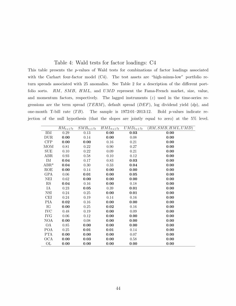
Table 4: Wald tests for factor loadings: C4This table presents the p-values of Wald tests for combinations of factor loadings associated
with the Carhart four-factor model (C4). The test assets are “high-minus-low” portfolio re-
turn spreads associated with 25 anomalies. See Table 2 for a description of the different port-
folio sorts. RM , SMB, HML, and UMD represent the Fama-French market, size, value,
and momentum factors, respectively. The lagged instruments (z) used in the time-series re-
gressions are the term spread (TERM), default spread (DEF ), log dividend yield (dp), and
one-month T-bill rate (TB). The sample is 1972:01–2013:12. Bold p-values indicate re-
jection of the null hypothesis (that the slopes are jointly equal to zero) at the 5% level.
RMt+1zt SMBt+1zt HMLt+1zt UMDt+1zt (RM,SMB,HML,UMD)BM 0.29 0.13 0.00 0.03 0.00
DUR 0.00 0.14 0.00 0.08 0.00CFP 0.00 0.00 0.16 0.21 0.00MOM 0.81 0.22 0.90 0.27 0.00SUE 0.10 0.22 0.09 0.21 0.00ABR 0.93 0.58 0.10 0.12 0.00IM 0.04 0.17 0.83 0.03 0.00
ABR* 0.04 0.30 0.33 0.04 0.00ROE 0.00 0.14 0.00 0.00 0.00GPA 0.06 0.01 0.00 0.05 0.00NEI 0.62 0.00 0.00 0.00 0.00RS 0.04 0.16 0.00 0.18 0.00IA 0.23 0.05 0.39 0.01 0.00
NSI 0.24 0.25 0.00 0.01 0.00CEI 0.24 0.19 0.14 0.16 0.00PIA 0.02 0.16 0.00 0.00 0.00IG 0.00 0.25 0.02 0.16 0.00
IVC 0.48 0.19 0.00 0.09 0.00IVG 0.06 0.12 0.00 0.00 0.00NOA 0.00 0.08 0.00 0.00 0.00OA 0.85 0.00 0.00 0.00 0.00
POA 0.25 0.01 0.01 0.14 0.00PTA 0.00 0.00 0.00 0.07 0.00OCA 0.00 0.03 0.00 0.58 0.00OL 0.00 0.00 0.00 0.00 0.00
44

Table 5: Wald tests for factor loadings: HXZ4This table presents the p-values of Wald tests for combinations of factor loadings associated
with the Hou-Xue-Zhang four-factor model (HXZ4). The test assets are “high-minus-low” port-
folio return spreads associated with 25 anomalies. See Table 2 for a description of the differ-
ent portfolio sorts. RM , ME, IA, and ROE represent the Hou-Xue-Zhang market, size, in-
vestment, and profitability factors, respectively. The lagged instruments (z) used in the time-
series regressions are the term spread (TERM), default spread (DEF ), log dividend yield
(dp), and one-month T-bill rate (TB). The sample is 1972:01–2013:12. Bold p-values indi-
cate rejection of the null hypothesis (that the slopes are jointly equal to zero) at the 5% level.
RMt+1zt MEt+1zt IAt+1zt ROEt+1zt (RM,ME, IA,ROE)BM 0.01 0.03 0.08 0.01 0.00
DUR 0.06 0.00 0.00 0.00 0.00CFP 0.57 0.00 0.08 0.00 0.00MOM 0.76 0.01 0.01 0.00 0.00SUE 0.00 0.07 0.56 0.05 0.00ABR 0.75 0.04 0.02 0.23 0.00IM 0.13 0.00 0.01 0.22 0.00
ABR* 0.04 0.00 0.01 0.16 0.00ROE 0.12 0.58 0.00 0.12 0.00GPA 0.01 0.05 0.01 0.11 0.00NEI 0.09 0.00 0.88 0.00 0.00RS 0.03 0.01 0.02 0.06 0.00IA 0.74 0.10 0.08 0.03 0.00
NSI 0.34 0.25 0.17 0.00 0.00CEI 0.91 0.14 0.77 0.04 0.00PIA 0.08 0.04 0.04 0.00 0.00IG 0.00 0.17 0.00 0.30 0.00
IVC 0.73 0.12 0.00 0.27 0.00IVG 0.03 0.18 0.02 0.00 0.00NOA 0.03 0.11 0.00 0.60 0.03OA 0.56 0.00 0.00 0.02 0.00
POA 0.26 0.00 0.13 0.02 0.00PTA 0.00 0.00 0.02 0.10 0.00OCA 0.00 0.05 0.15 0.04 0.00OL 0.00 0.00 0.00 0.00 0.00
45

Table 6: Wald tests for factor loadings: FF5This table presents the p-values of Wald tests for combinations of factor loadings associated
with the Fama-French five-factor model (FF5). The test assets are “high-minus-low” portfo-
lio return spreads associated with 25 anomalies. See Table 2 for a description of the differ-
ent portfolio sorts. RM , SMB, HML, RMW , and CMA represent the Fama-French market,
size, value, profitability, and investment factors, respectively. The lagged instruments (z) used
in the time-series regressions are the term spread (TERM), default spread (DEF ), log dividend
yield (dp), and one-month T-bill rate (TB). The sample is 1972:01–2013:12. Bold p-values indi-
cate rejection of the null hypothesis (that the slopes are jointly equal to zero) at the 5% level.
RMt+1zt SMBt+1zt HMLt+1zt RMWt+1zt CMAt+1zt (RM,SMB,HML,RMW,CMA)BM 0.47 0.25 0.01 0.06 0.04 0.00
DUR 0.01 0.22 0.00 0.00 0.46 0.00CFP 0.00 0.00 0.36 0.01 0.38 0.00MOM 0.04 0.06 0.15 0.00 0.01 0.08SUE 0.02 0.02 0.09 0.12 0.45 0.77ABR 0.17 0.34 0.01 0.08 0.14 0.09IM 0.07 0.14 0.22 0.00 0.08 0.85
ABR* 0.10 0.08 0.15 0.06 0.05 0.13ROE 0.00 0.64 0.05 0.00 0.48 0.00GPA 0.01 0.04 0.02 0.43 0.00 0.00NEI 0.27 0.00 0.09 0.10 0.53 0.00RS 0.06 0.24 0.02 0.77 0.11 0.00IA 0.43 0.00 0.03 0.21 0.00 0.00NSI 0.02 0.53 0.00 0.33 0.76 0.00CEI 0.16 0.21 0.16 0.37 0.24 0.00PIA 0.00 0.01 0.05 0.82 0.05 0.00IG 0.00 0.28 0.70 0.23 0.05 0.00
IVC 0.40 0.01 0.01 0.94 0.03 0.00IVG 0.14 0.08 0.08 0.77 0.29 0.00NOA 0.20 0.08 0.00 0.00 0.00 0.00OA 0.60 0.00 0.54 0.04 0.01 0.00
POA 0.42 0.00 0.80 0.47 0.21 0.00PTA 0.03 0.00 0.04 0.29 0.13 0.00OCA 0.00 0.78 0.03 0.00 0.27 0.00OL 0.00 0.10 0.01 0.15 0.01 0.00
46
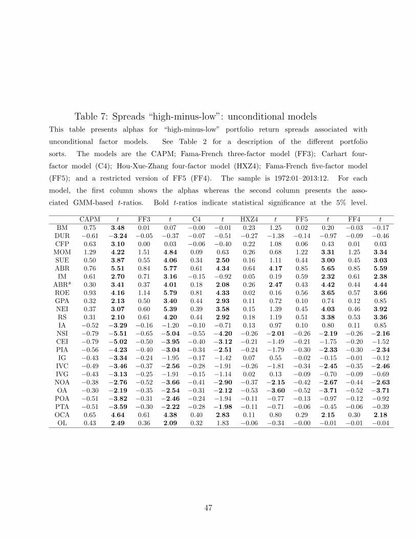
Table 7: Spreads “high-minus-low”: unconditional modelsThis table presents alphas for “high-minus-low” portfolio return spreads associated with
unconditional factor models. See Table 2 for a description of the different portfolio
sorts. The models are the CAPM; Fama-French three-factor model (FF3); Carhart four-
factor model (C4); Hou-Xue-Zhang four-factor model (HXZ4); Fama-French five-factor model
(FF5); and a restricted version of FF5 (FF4). The sample is 1972:01–2013:12. For each
model, the first column shows the alphas whereas the second column presents the asso-
ciated GMM-based t-ratios. Bold t-ratios indicate statistical significance at the 5% level.
CAPM t FF3 t C4 t HXZ4 t FF5 t FF4 tBM 0.75 3.48 0.01 0.07 −0.00 −0.01 0.23 1.25 0.02 0.20 −0.03 −0.17
DUR −0.61 −3.24 −0.05 −0.37 −0.07 −0.51 −0.27 −1.38 −0.14 −0.97 −0.09 −0.46CFP 0.63 3.10 0.00 0.03 −0.06 −0.40 0.22 1.08 0.06 0.43 0.01 0.03MOM 1.29 4.22 1.51 4.84 0.09 0.63 0.26 0.68 1.22 3.31 1.25 3.34SUE 0.50 3.87 0.55 4.06 0.34 2.50 0.16 1.11 0.44 3.00 0.45 3.03ABR 0.76 5.51 0.84 5.77 0.61 4.34 0.64 4.17 0.85 5.65 0.85 5.59IM 0.61 2.70 0.71 3.16 −0.15 −0.92 0.05 0.19 0.59 2.32 0.61 2.38
ABR* 0.30 3.41 0.37 4.01 0.18 2.08 0.26 2.47 0.43 4.42 0.44 4.44ROE 0.93 4.16 1.14 5.79 0.81 4.33 0.02 0.16 0.56 3.65 0.57 3.66GPA 0.32 2.13 0.50 3.40 0.44 2.93 0.11 0.72 0.10 0.74 0.12 0.85NEI 0.37 3.07 0.60 5.39 0.39 3.58 0.15 1.39 0.45 4.03 0.46 3.92RS 0.31 2.10 0.61 4.20 0.44 2.92 0.18 1.19 0.51 3.38 0.53 3.36IA −0.52 −3.29 −0.16 −1.20 −0.10 −0.71 0.13 0.97 0.10 0.80 0.11 0.85NSI −0.79 −5.51 −0.65 −5.04 −0.55 −4.20 −0.26 −2.01 −0.26 −2.19 −0.26 −2.16CEI −0.79 −5.02 −0.50 −3.95 −0.40 −3.12 −0.21 −1.49 −0.21 −1.75 −0.20 −1.52PIA −0.56 −4.23 −0.40 −3.04 −0.34 −2.51 −0.24 −1.79 −0.30 −2.33 −0.30 −2.34IG −0.43 −3.34 −0.24 −1.95 −0.17 −1.42 0.07 0.55 −0.02 −0.15 −0.01 −0.12
IVC −0.49 −3.46 −0.37 −2.56 −0.28 −1.91 −0.26 −1.81 −0.34 −2.45 −0.35 −2.46IVG −0.43 −3.13 −0.25 −1.91 −0.15 −1.14 0.02 0.13 −0.09 −0.70 −0.09 −0.69NOA −0.38 −2.76 −0.52 −3.66 −0.41 −2.90 −0.37 −2.15 −0.42 −2.67 −0.44 −2.63OA −0.30 −2.19 −0.35 −2.54 −0.31 −2.12 −0.53 −3.60 −0.52 −3.71 −0.52 −3.71
POA −0.51 −3.82 −0.31 −2.46 −0.24 −1.94 −0.11 −0.77 −0.13 −0.97 −0.12 −0.92PTA −0.51 −3.59 −0.30 −2.22 −0.28 −1.98 −0.11 −0.71 −0.06 −0.45 −0.06 −0.39OCA 0.65 4.64 0.61 4.38 0.40 2.83 0.11 0.80 0.29 2.15 0.30 2.18OL 0.43 2.49 0.36 2.09 0.32 1.83 −0.06 −0.34 −0.00 −0.01 −0.01 −0.04
47

Table 8: Spreads “high-minus-low”: conditional modelsThis table presents alphas for “high-minus-low” portfolio return spreads associated with con-
ditional factor models. See Table 2 for a description of the different portfolio sorts.
The models are the CAPM; Fama-French three-factor model (FF3); Carhart four-factor
model (C4); Hou-Xue-Zhang four-factor model (HXZ4); Fama-French five-factor model
(FF5); and a restricted version of FF5 (FF4). The lagged instruments used in the
time-series regressions are the term spread (TERM), default spread (DEF ), log dividend
yield (dp), and one-month T-bill rate (TB). The sample is 1972:01–2013:12. For each
model, the first column shows the alphas whereas the second column presents the asso-
ciated GMM-based t-ratios. Bold t-ratios indicate statistical significance at the 5% level.
CAPM t FF3 t C4 t HXZ4 t FF5 t FF4 tBM 0.62 3.00 −0.07 −0.59 −0.11 −0.80 0.38 2.08 −0.01 −0.11 0.12 0.72
DUR −0.59 −3.14 −0.05 −0.36 −0.01 −0.08 −0.32 −1.84 0.07 0.48 −0.06 −0.32CFP 0.57 2.89 0.03 0.23 −0.04 −0.25 0.40 2.05 −0.08 −0.54 0.05 0.24MOM 1.35 4.43 1.40 4.46 0.10 0.76 0.07 0.22 0.93 2.61 0.89 2.57SUE 0.48 3.71 0.47 3.57 0.30 2.23 0.04 0.28 0.40 2.80 0.38 2.70ABR 0.77 5.53 0.81 5.63 0.62 4.44 0.54 3.51 0.80 5.56 0.77 5.21IM 0.64 2.86 0.63 2.75 −0.19 −1.23 −0.16 −0.67 0.34 1.31 0.34 1.35
ABR* 0.34 3.78 0.36 3.95 0.20 2.21 0.13 1.34 0.36 3.63 0.33 3.38ROE 0.87 4.28 1.20 7.97 0.87 6.39 0.21 1.71 0.84 5.64 0.78 5.16GPA 0.27 1.83 0.54 4.18 0.45 3.37 0.10 0.72 0.12 0.93 0.04 0.33NEI 0.37 3.08 0.59 5.42 0.33 3.12 −0.01 −0.06 0.41 3.72 0.36 3.17RS 0.33 2.18 0.63 4.64 0.45 3.22 0.01 0.08 0.53 3.57 0.44 2.88IA −0.41 −2.72 −0.10 −0.77 −0.08 −0.59 −0.02 −0.17 0.03 0.26 0.04 0.38NSI −0.75 −5.30 −0.62 −4.94 −0.58 −4.64 −0.41 −3.17 −0.19 −1.59 −0.22 −1.87CEI −0.73 −4.61 −0.47 −3.75 −0.38 −2.99 −0.28 −2.00 −0.07 −0.59 −0.12 −0.92PIA −0.53 −4.00 −0.31 −2.48 −0.30 −2.32 −0.15 −1.24 −0.23 −1.99 −0.23 −1.95IG −0.41 −3.23 −0.18 −1.55 −0.14 −1.18 0.03 0.26 −0.07 −0.62 −0.08 −0.71
IVC −0.49 −3.43 −0.33 −2.36 −0.26 −1.83 −0.18 −1.27 −0.28 −2.07 −0.27 −2.00IVG −0.41 −2.99 −0.19 −1.41 −0.08 −0.66 0.01 0.11 −0.06 −0.50 −0.10 −0.85NOA −0.39 −2.79 −0.48 −3.61 −0.44 −3.28 −0.32 −2.00 −0.39 −2.71 −0.40 −2.69OA −0.32 −2.42 −0.22 −1.68 −0.14 −1.07 −0.27 −1.90 −0.28 −2.02 −0.30 −2.21
POA −0.44 −3.33 −0.23 −1.89 −0.14 −1.20 −0.17 −1.28 −0.11 −0.85 −0.12 −0.95PTA −0.43 −2.98 −0.21 −1.61 −0.20 −1.49 −0.20 −1.43 0.00 0.00 −0.04 −0.32OCA 0.59 4.82 0.64 5.14 0.49 3.94 0.28 2.08 0.43 3.27 0.38 2.92OL 0.36 2.19 0.33 2.16 0.38 2.47 0.13 0.77 0.06 0.41 0.09 0.61
48

Table 9: Joint time-series tests by category: unconditional modelsThis table presents joint time-series tests of unconditional factor models. The test portfolios are combina-
tions of 25 different portfolios sorts that correspond to the categories defined in Table 2. For example, the
value-growth category contains the BM, DUR, and CFP deciles. In Panel F all the 25 sorts are included simul-
taneously as test assets. See Table 2 for a description of the different portfolio sorts and categories. The mod-
els are the CAPM; Fama-French three-factor model (FF3); Carhart four-factor model (C4); Hou-Xue-Zhang
four-factor model (HXZ4); Fama-French five-factor model (FF5); and a restricted version of FF5 (FF4). The
sample is 1972:01–2013:12. MAA denotes the mean absolute alpha and RMSA is the root mean squared
alpha. # < 0.05 represents the number of portfolios in which the alphas are significant at the 5% level. F
and χ2 denote the p-values associated with the GRS and robust χ2 model specification tests, respectively.
CAPM FF3 C4 HXZ4 FF5 FF4Panel A (Value-growth)
MAA 0.21 0.08 0.07 0.10 0.07 0.07RMSA 0.25 0.09 0.08 0.13 0.09 0.09
# < 0.05 16 3 2 2 1 1F 0.05 0.10 0.38 0.03 0.14 0.15χ2 0.02 0.05 0.27 0.01 0.08 0.09
Panel B (Momentum)MAA 0.15 0.17 0.09 0.10 0.16 0.17RMSA 0.21 0.24 0.13 0.14 0.21 0.22
# < 0.05 17 20 11 7 15 15F 0.00 0.00 0.00 0.00 0.00 0.00χ2 0.00 0.00 0.00 0.00 0.00 0.00
Panel C (Profitability)MAA 0.12 0.18 0.13 0.09 0.12 0.12RMSA 0.16 0.22 0.16 0.12 0.15 0.15
# < 0.05 7 18 8 7 9 9F 0.03 0.00 0.01 0.05 0.06 0.12χ2 0.01 0.00 0.00 0.02 0.02 0.05
Panel D (Investment)MAA 0.15 0.12 0.11 0.11 0.10 0.10RMSA 0.18 0.15 0.13 0.14 0.13 0.13
# < 0.05 37 28 23 20 26 27F 0.01 0.00 0.04 0.00 0.00 0.00χ2 0.00 0.00 0.00 0.00 0.00 0.00
Panel E (Intangibles)MAA 0.12 0.12 0.11 0.12 0.10 0.10RMSA 0.15 0.15 0.13 0.15 0.12 0.12
# < 0.05 5 6 4 3 3 4F 0.03 0.00 0.02 0.08 0.05 0.08χ2 0.02 0.00 0.01 0.05 0.03 0.05
Panel F (All)MAA 0.15 0.13 0.10 0.11 0.11 0.11RMSA 0.19 0.18 0.13 0.14 0.15 0.15
# < 0.05 82 75 48 39 54 56F 0.00 0.00 0.00 0.00 0.00 0.00χ2 0.00 0.00 0.00 0.00 0.00 0.00
49

Table 10: Joint time-series tests by category: conditional modelsThis table presents joint time-series tests of conditional factor models. The test portfolios are combina-
tions of 25 different portfolios sorts that correspond to the categories defined in Table 2. For example,
the value-growth category contains the BM, DUR, and CFP deciles. In Panel F all the 25 sorts are in-
cluded simultaneously as test assets. See Table 2 for a description of the different portfolio sorts and
categories. The models are the CAPM; Fama-French three-factor model (FF3); Carhart four-factor model
(C4); Hou-Xue-Zhang four-factor model (HXZ4); Fama-French five-factor model (FF5); and a restricted
version of FF5 (FF4). The lagged instruments used in the time-series regressions are the term spread
(TERM), default spread (DEF ), log dividend yield (dp), and one-month T-bill rate (TB). The sample
is 1972:01–2013:12. MAA denotes the mean absolute alpha and RMSA is the root mean squared al-
pha. # < 0.05 represents the number of portfolios in which the alphas are significant at the 5% level. F
and χ2 denote the p-values associated with the GRS and robust χ2 model specification tests, respectively.
CAPM FF3 C4 HXZ4 FF5 FF4Panel A (Value-growth)
MAA 0.18 0.07 0.06 0.13 0.06 0.07RMSA 0.21 0.09 0.08 0.16 0.07 0.08
# < 0.05 11 4 3 7 1 0F 0.06 0.13 0.22 0.18 0.78 0.75χ2 0.03 0.05 0.11 0.08 0.64 0.62
Panel B (Momentum)MAA 0.14 0.15 0.09 0.09 0.11 0.11RMSA 0.21 0.22 0.13 0.12 0.16 0.15
# < 0.05 14 19 11 5 8 9F 0.00 0.00 0.00 0.01 0.00 0.00χ2 0.00 0.00 0.00 0.00 0.00 0.00
Panel C (Profitability)MAA 0.12 0.18 0.14 0.09 0.13 0.11RMSA 0.16 0.23 0.17 0.11 0.16 0.15
# < 0.05 7 19 10 6 8 8F 0.02 0.00 0.00 0.06 0.00 0.03χ2 0.00 0.00 0.00 0.01 0.00 0.00
Panel D (Investment)MAA 0.13 0.10 0.10 0.10 0.08 0.09RMSA 0.16 0.13 0.12 0.12 0.11 0.11
# < 0.05 31 28 22 14 15 12F 0.01 0.01 0.05 0.01 0.02 0.02χ2 0.00 0.00 0.00 0.00 0.00 0.00
Panel E (Intangibles)MAA 0.10 0.11 0.11 0.10 0.09 0.08RMSA 0.13 0.15 0.14 0.12 0.11 0.10
# < 0.05 4 5 5 1 2 1F 0.01 0.00 0.00 0.09 0.08 0.23χ2 0.01 0.00 0.00 0.05 0.04 0.14
Panel F (All)MAA 0.13 0.12 0.10 0.10 0.09 0.09RMSA 0.18 0.17 0.13 0.13 0.13 0.12
# < 0.05 67 75 51 33 34 30F 0.00 0.00 0.00 0.00 0.00 0.00χ2 0.00 0.00 0.00 0.00 0.00 0.00
50

Table 11: Time-series tests by category: extreme decilesThis table presents joint time-series tests of conditional factor models. The test portfolios are combi-
nations of 25 different portfolios sorts that correspond to the categories defined in Table 2. For ex-
ample, the value-growth category contains the BM, DUR, and CFP deciles. For each anomaly, only
the extreme first and last deciles are considered. In Panel F all the 25 sorts are included simulta-
neously as test assets. See Table 2 for a description of the different portfolio sorts and categories.
The models are the CAPM; Fama-French three-factor model (FF3); Carhart four-factor model (C4);
Hou-Xue-Zhang four-factor model (HXZ4); Fama-French five-factor model (FF5); and a restricted ver-
sion of FF5 (FF4). The lagged instruments used in the time-series regressions are the term spread
(TERM), default spread (DEF ), log dividend yield (dp), and one-month T-bill rate (TB). The sample
is 1972:01–2013:12. MAA denotes the mean absolute alpha and RMSA is the root mean squared al-
pha. # < 0.05 represents the number of portfolios in which the alphas are significant at the 5% level. F
and χ2 denote the p-values associated with the GRS and robust χ2 model specification tests, respectively.
CAPM FF3 C4 HXZ4 FF5 FF4Panel A (Value-growth)
MAA 0.30 0.09 0.08 0.18 0.08 0.08RMSA 0.31 0.10 0.09 0.23 0.09 0.10
# < 0.05 3 1 0 2 1 0F 0.00 0.00 0.01 0.01 0.06 0.11χ2 0.00 0.00 0.00 0.01 0.04 0.09
Panel B (Momentum)MAA 0.36 0.37 0.14 0.13 0.28 0.27RMSA 0.41 0.42 0.18 0.16 0.31 0.30
# < 0.05 7 8 3 2 5 5F 0.00 0.00 0.00 0.01 0.00 0.00χ2 0.00 0.00 0.00 0.00 0.00 0.00
Panel C (Profitability)MAA 0.23 0.37 0.26 0.10 0.26 0.24RMSA 0.28 0.40 0.29 0.11 0.29 0.26
# < 0.05 4 8 5 0 7 6F 0.01 0.00 0.00 0.07 0.00 0.00χ2 0.01 0.00 0.00 0.05 0.00 0.00
Panel D (Investment)MAA 0.25 0.17 0.14 0.11 0.10 0.11RMSA 0.27 0.20 0.17 0.12 0.12 0.12
# < 0.05 14 9 8 2 3 2F 0.00 0.00 0.01 0.29 0.10 0.15χ2 0.00 0.00 0.00 0.19 0.04 0.08
Panel E (Intangibles)MAA 0.24 0.24 0.22 0.10 0.13 0.12RMSA 0.25 0.26 0.22 0.12 0.16 0.16
# < 0.05 2 3 3 0 1 1F 0.00 0.00 0.00 0.15 0.01 0.02χ2 0.00 0.00 0.00 0.13 0.01 0.02
Panel F (All)MAA 0.27 0.24 0.16 0.12 0.16 0.16RMSA 0.31 0.29 0.20 0.15 0.21 0.20
# < 0.05 30 29 19 6 17 14F 0.00 0.00 0.00 0.00 0.00 0.00χ2 0.00 0.00 0.00 0.00 0.00 0.00
51

Table 12: Time-series tests by category: intermediate decilesThis table presents joint time-series tests of conditional factor models. The test portfolios are combina-
tions of 25 different portfolios sorts that correspond to the categories defined in Table 2. For example,
the value-growth category contains the BM, DUR, and CFP deciles. For each anomaly, all the port-
folios are included except the extreme first and last deciles. In Panel F all the 25 sorts are included
simultaneously as test assets. See Table 2 for a description of the different portfolio sorts and cate-
gories. The models are the CAPM; Fama-French three-factor model (FF3); Carhart four-factor model
(C4); Hou-Xue-Zhang four-factor model (HXZ4); Fama-French five-factor model (FF5); and a restricted
version of FF5 (FF4). The lagged instruments used in the time-series regressions are the term spread
(TERM), default spread (DEF ), log dividend yield (dp), and one-month T-bill rate (TB). The sample
is 1972:01–2013:12. MAA denotes the mean absolute alpha and RMSA is the root mean squared al-
pha. # < 0.05 represents the number of portfolios in which the alphas are significant at the 5% level. F
and χ2 denote the p-values associated with the GRS and robust χ2 model specification tests, respectively.
CAPM FF3 C4 HXZ4 FF5 FF4Panel A (Value-growth)
MAA 0.14 0.07 0.06 0.11 0.05 0.07RMSA 0.18 0.08 0.08 0.14 0.06 0.08
# < 0.05 8 3 3 5 0 0F 0.04 0.19 0.31 0.15 0.84 0.71χ2 0.02 0.11 0.20 0.08 0.76 0.60
Panel B (Momentum)MAA 0.09 0.09 0.08 0.08 0.07 0.07RMSA 0.11 0.11 0.11 0.11 0.08 0.08
# < 0.05 7 11 8 3 3 4F 0.09 0.00 0.00 0.08 0.04 0.06χ2 0.03 0.00 0.00 0.02 0.01 0.01
Panel C (Profitability)MAA 0.09 0.13 0.10 0.09 0.09 0.08RMSA 0.11 0.16 0.12 0.12 0.11 0.10
# < 0.05 3 11 5 6 1 2F 0.36 0.01 0.04 0.06 0.21 0.39χ2 0.25 0.00 0.01 0.02 0.09 0.23
Panel D (Investment)MAA 0.10 0.09 0.09 0.09 0.08 0.08RMSA 0.12 0.11 0.11 0.12 0.10 0.11
# < 0.05 17 19 14 12 12 10F 0.09 0.10 0.14 0.01 0.02 0.02χ2 0.00 0.00 0.00 0.00 0.00 0.00
Panel E (Intangibles)MAA 0.06 0.08 0.09 0.10 0.07 0.07RMSA 0.08 0.11 0.11 0.11 0.09 0.08
# < 0.05 2 2 2 1 1 0F 0.00 0.12 0.29 0.47 0.53 0.72χ2 0.00 0.08 0.22 0.39 0.44 0.65
Panel F (All)MAA 0.10 0.09 0.08 0.09 0.08 0.08RMSA 0.12 0.12 0.11 0.12 0.10 0.10
# < 0.05 37 46 32 27 17 16F 0.03 0.04 0.03 0.01 0.06 0.07χ2 0.00 0.00 0.00 0.00 0.00 0.00
52

Table 13: Time-series tests for conditional models: individual anomaliesThis table presents time-series tests of conditional factor models for selected individual anomalies. The portfolios are sorted
on BM, MOM, ROE, NSI, OCA, ABR, CEI, DUR, and IM. See Table 2 for a description of the different portfolio sorts.
The models are the CAPM; Fama-French three-factor model (FF3); Carhart four-factor model (C4); Hou-Xue-Zhang four-
factor model (HXZ4); Fama-French five-factor model (FF5); and a restricted version of FF5 (FF4). The lagged instru-
ments used in the time-series regressions are the term spread (TERM), default spread (DEF ), log dividend yield (dp),
and one-month T-bill rate (TB). The sample is 1972:01–2013:12. MAA denotes the mean absolute alpha and RMSA is
the root mean squared alpha. # < 0.05 represents the number of portfolios in which the alphas are significant at the
5% level. F and χ2 denote the p-values associated with the GRS and robust χ2 model specification tests, respectively.
BM DUR MOM ABR IM ROE NSI CEI OCAPanel A (CAPM)
MAA 0.17 0.20 0.22 0.13 0.14 0.16 0.16 0.16 0.12RMSA 0.21 0.23 0.33 0.19 0.18 0.24 0.20 0.21 0.16
# < 0.05 4 5 4 3 1 3 4 4 4F 0.14 0.02 0.00 0.00 0.09 0.01 0.00 0.00 0.00χ2 0.12 0.02 0.00 0.00 0.08 0.00 0.00 0.00 0.00
Panel B (FF3)MAA 0.05 0.10 0.23 0.13 0.13 0.26 0.15 0.12 0.14RMSA 0.06 0.11 0.34 0.20 0.18 0.34 0.18 0.16 0.19
# < 0.05 0 3 4 3 4 7 4 3 4F 0.23 0.06 0.00 0.00 0.21 0.00 0.00 0.00 0.00χ2 0.19 0.04 0.00 0.00 0.17 0.00 0.00 0.00 0.00
Panel C (C4)MAA 0.05 0.09 0.14 0.11 0.06 0.18 0.13 0.11 0.12RMSA 0.06 0.10 0.19 0.16 0.07 0.23 0.16 0.14 0.15
# < 0.05 0 2 4 3 1 4 3 3 4F 0.31 0.14 0.00 0.00 0.31 0.00 0.00 0.00 0.00χ2 0.26 0.10 0.00 0.00 0.26 0.00 0.00 0.00 0.00
Panel D (HXZ4)MAA 0.13 0.13 0.14 0.10 0.06 0.12 0.11 0.11 0.11RMSA 0.16 0.15 0.16 0.15 0.08 0.14 0.14 0.12 0.12
# < 0.05 2 3 1 2 0 4 2 0 1F 0.16 0.21 0.04 0.00 0.17 0.00 0.00 0.08 0.07χ2 0.13 0.17 0.02 0.00 0.14 0.00 0.00 0.06 0.05
Panel E (FF5)MAA 0.05 0.07 0.13 0.13 0.11 0.18 0.11 0.09 0.11RMSA 0.05 0.07 0.22 0.19 0.13 0.23 0.12 0.10 0.13
# < 0.05 0 0 1 3 1 2 2 1 1F 0.89 0.74 0.00 0.00 0.10 0.00 0.01 0.10 0.03χ2 0.86 0.69 0.00 0.00 0.07 0.00 0.01 0.07 0.02
Panel F (FF4)MAA 0.07 0.07 0.12 0.12 0.13 0.16 0.10 0.09 0.10RMSA 0.08 0.08 0.21 0.19 0.14 0.21 0.13 0.10 0.12
# < 0.05 0 0 1 3 3 2 2 1 1F 0.92 0.66 0.00 0.00 0.04 0.00 0.03 0.12 0.05χ2 0.91 0.61 0.00 0.00 0.03 0.00 0.01 0.09 0.03
53
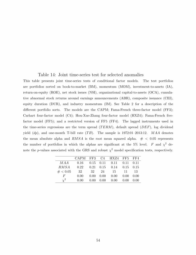
Table 14: Joint time-series test for selected anomaliesThis table presents joint time-series tests of conditional factor models. The test portfolios
are portfolios sorted on book-to-market (BM), momentum (MOM), investment-to-assets (IA),
return-on-equity (ROE), net stock issues (NSI), organizational capital-to-assets (OCA), cumula-
tive abnormal stock returns around earnings announcements (ABR), composite issuance (CEI),
equity duration (DUR), and industry momentum (IM). See Table 2 for a description of the
different portfolio sorts. The models are the CAPM; Fama-French three-factor model (FF3);
Carhart four-factor model (C4); Hou-Xue-Zhang four-factor model (HXZ4); Fama-French five-
factor model (FF5); and a restricted version of FF5 (FF4). The lagged instruments used in
the time-series regressions are the term spread (TERM), default spread (DEF ), log dividend
yield (dp), and one-month T-bill rate (TB). The sample is 1972:01–2013:12. MAA denotes
the mean absolute alpha and RMSA is the root mean squared alpha. # < 0.05 represents
the number of portfolios in which the alphas are significant at the 5% level. F and χ2 de-
note the p-values associated with the GRS and robust χ2 model specification tests, respectively.
CAPM FF3 C4 HXZ4 FF5 FF4
MAA 0.16 0.15 0.11 0.11 0.11 0.11RMSA 0.22 0.21 0.15 0.14 0.15 0.15
# < 0.05 32 32 24 15 11 13F 0.00 0.00 0.00 0.00 0.00 0.00χ2 0.00 0.00 0.00 0.00 0.00 0.00
54

Table 15: Decomposition of spreads high-minus-low: C4This table reports the risk premium (beta times risk price) for each factor from the Carhart four-
factor model (C4) when tested on the spreads high-minus-low in average returns. The spreads are
associated with portfolios sorted on BM, MOM, ROE, NSI, OCA, ABR, CEI, DUR, and IM. See
Table 2 for a description of the different portfolio sorts. E(R) denotes the original spread in av-
erage returns, and α represents the corresponding alpha. RM , SMB, HML, and UMD repre-
sent the market, size, value, and momentum factors, respectively. The lagged instruments used in
the time-series regressions are the term spread (TERM), default spread (DEF ), log dividend yield
(dp), and one-month T-bill rate (TB). The sample is 1972:01–2013:12. All the numbers are in %
BM DUR MOM ABR IM ROE NSI CEI OCAE(R) 0.69 -0.52 1.17 0.73 0.54 0.75 -0.69 -0.55 0.55RMt+1 0.04 0.00 0.00 -0.01 0.02 -0.12 0.02 0.11 -0.08
RMt+1TERMt 0.01 0.05 -0.02 0.00 -0.04 -0.04 0.01 0.00 -0.02RMt+1DEFt -0.01 -0.01 0.00 -0.01 -0.01 0.00 0.01 0.01 -0.04RMt+1dpt 0.02 0.01 0.00 0.01 0.02 0.03 0.01 0.00 0.05RMt+1TBt 0.00 0.01 0.00 0.00 0.04 0.00 0.02 0.02 0.03SMBt+1 0.12 -0.06 -0.01 -0.01 0.00 -0.14 0.04 0.06 0.02
SMBt+1TERMt -0.03 0.04 0.04 0.04 0.03 -0.04 0.00 0.01 -0.06SMBt+1DEFt 0.02 0.00 -0.01 -0.02 0.00 0.02 -0.01 -0.02 0.02SMBt+1dpt -0.01 -0.02 0.00 -0.01 -0.02 0.02 -0.01 0.01 0.01SMBt+1TBt 0.01 -0.03 -0.01 -0.02 -0.03 0.03 -0.01 -0.01 0.03HMLt+1 0.57 -0.44 0.02 -0.03 0.04 -0.17 -0.11 -0.28 0.01
HMLt+1TERMt 0.00 -0.01 0.00 -0.01 0.00 -0.01 0.01 0.01 0.01HMLt+1DEFt 0.02 -0.01 -0.01 -0.01 0.01 -0.04 0.02 0.01 -0.01HMLt+1dpt 0.00 0.00 0.00 0.00 0.00 0.01 -0.01 0.00 0.00HMLt+1TBt 0.02 -0.01 0.01 0.03 0.01 0.06 -0.07 -0.04 -0.02UMDt+1 0.01 -0.03 1.05 0.16 0.64 0.27 -0.04 -0.07 0.13
UMDt+1TERMt 0.02 0.02 0.02 0.02 0.04 -0.03 0.01 -0.01 -0.01UMDt+1DEFt 0.02 -0.02 0.01 0.03 0.04 0.00 0.05 0.00 -0.02UMDt+1dpt -0.01 0.01 0.00 -0.01 -0.01 -0.01 -0.01 0.01 0.01UMDt+1TBt -0.01 -0.02 -0.04 -0.05 -0.05 0.02 -0.03 0.01 0.02
α -0.11 -0.01 0.10 0.62 -0.19 0.87 -0.58 -0.38 0.49
55
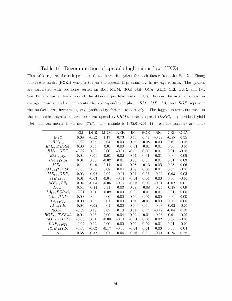
Table 16: Decomposition of spreads high-minus-low: HXZ4This table reports the risk premium (beta times risk price) for each factor from the Hou-Xue-Zhang
four-factor model (HXZ4) when tested on the spreads high-minus-low in average returns. The spreads
are associated with portfolios sorted on BM, MOM, ROE, NSI, OCA, ABR, CEI, DUR, and IM.
See Table 2 for a description of the different portfolio sorts. E(R) denotes the original spread in
average returns, and α represents the corresponding alpha. RM , ME, IA, and ROE represent
the market, size, investment, and profitability factors, respectively. The lagged instruments used in
the time-series regressions are the term spread (TERM), default spread (DEF ), log dividend yield
(dp), and one-month T-bill rate (TB). The sample is 1972:01–2013:12. All the numbers are in %
BM DUR MOM ABR IM ROE NSI CEI OCAE(R) 0.69 -0.52 1.17 0.73 0.54 0.75 -0.69 -0.55 0.55RMt+1 -0.02 0.06 0.04 0.00 0.03 -0.08 0.00 0.10 -0.06
RMt+1TERMt 0.00 0.04 -0.01 0.00 -0.04 -0.01 0.01 0.00 -0.03RMt+1DEFt -0.02 0.00 0.00 -0.01 -0.01 0.00 0.01 0.01 -0.04RMt+1dpt 0.04 -0.01 -0.03 0.02 0.01 0.02 0.01 0.00 0.05RMt+1TBt 0.01 0.00 -0.02 0.01 0.03 0.01 0.01 0.01 0.03MEt+1 0.14 -0.10 0.11 0.01 0.08 -0.13 0.05 0.08 0.06
MEt+1TERMt -0.05 0.06 0.08 0.04 0.07 0.00 0.01 0.04 -0.03MEt+1DEFt 0.03 -0.02 0.02 -0.01 0.01 0.02 -0.02 -0.03 0.03MEt+1dpt 0.01 -0.03 -0.04 -0.01 -0.04 0.00 0.00 0.00 -0.01MEt+1TBt 0.04 -0.05 -0.06 -0.04 -0.06 0.00 -0.01 -0.02 0.01IAt+1 0.54 -0.34 0.31 0.03 0.18 -0.08 -0.25 -0.45 0.09
IAt+1TERMt -0.01 0.01 -0.02 0.00 -0.01 -0.01 0.01 0.01 0.00IAt+1DEFt 0.00 0.00 0.00 0.00 0.00 0.00 0.00 0.00 0.00IAt+1dpt 0.00 0.00 0.01 0.00 0.01 -0.01 0.00 0.00 0.00IAt+1TBt 0.03 -0.05 0.01 0.00 0.00 0.01 -0.03 -0.02 -0.01ROEt+1 -0.39 0.19 0.87 0.18 0.51 0.77 -0.12 -0.04 0.18
ROEt+1TERMt 0.04 0.03 0.09 0.04 0.02 -0.01 -0.03 -0.01 -0.02ROEt+1DEFt -0.03 0.01 -0.09 -0.01 -0.04 0.00 0.02 0.02 -0.03ROEt+1dpt -0.02 0.02 0.00 0.00 0.00 0.00 0.01 0.01 -0.01ROEt+1TBt -0.03 -0.02 -0.17 -0.06 -0.04 0.04 0.06 0.03 0.04
α 0.38 -0.32 0.07 0.54 -0.16 0.21 -0.41 -0.28 0.28
56

Table 17: Decomposition of spreads high-minus-low: FF5This table reports the risk premium (beta times risk price) for each factor from the Fama-French five-
factor model (FF5) when tested on the spreads high-minus-low in average returns. The spreads are
associated with portfolios sorted on BM, MOM, ROE, NSI, OCA, ABR, CEI, DUR, and IM. See Ta-
ble 2 for a description of the different portfolio sorts. E(R) denotes the original spread in average re-
turns, and α represents the corresponding alpha. RM , SMB, HML, RMW , and CMA represent
the market, size, value, profitability, and investment factors, respectively. The lagged instruments used
in the time-series regressions are the term spread (TERM), default spread (DEF ), log dividend yield
(dp), and one-month T-bill rate (TB). The sample is 1972:01–2013:12. All the numbers are in %
BM DUR MOM ABR IM ROE NSI CEI OCAE(R) 0.69 -0.52 1.17 0.73 0.54 0.75 -0.69 -0.55 0.55RMt+1 0.04 0.00 -0.01 -0.03 0.00 -0.09 -0.03 0.05 -0.07
RMt+1TERMt -0.01 0.04 0.03 0.02 -0.01 -0.03 0.01 0.01 -0.02RMt+1DEFt 0.00 0.00 -0.06 -0.02 -0.05 -0.01 0.01 0.01 -0.05RMt+1dpt 0.02 0.01 0.01 0.02 0.03 0.03 0.02 0.01 0.05RMt+1TBt 0.01 0.01 -0.06 -0.01 0.01 0.01 0.02 0.02 0.02SMBt+1 0.10 -0.07 -0.02 -0.01 -0.01 -0.12 0.02 0.06 0.03
SMBt+1TERMt -0.05 0.02 0.20 0.07 0.15 0.03 -0.03 -0.01 -0.02SMBt+1DEFt 0.03 0.01 -0.09 -0.03 -0.05 -0.01 0.00 -0.01 0.01SMBt+1dpt 0.01 -0.02 -0.02 -0.01 -0.04 -0.01 0.00 0.02 -0.01SMBt+1TBt 0.02 -0.02 -0.07 -0.03 -0.07 -0.01 0.02 0.01 0.01HMLt+1 0.53 -0.48 -0.09 -0.06 -0.02 -0.16 -0.05 -0.19 -0.07
HMLt+1TERMt -0.02 0.00 -0.01 -0.02 0.00 -0.01 0.00 0.00 0.00HMLt+1DEFt 0.02 0.00 0.01 -0.02 0.02 -0.02 0.02 0.01 -0.02HMLt+1dpt 0.00 0.00 -0.01 0.01 0.00 0.01 0.00 0.00 0.00HMLt+1TBt 0.06 -0.03 -0.09 0.05 -0.06 0.07 -0.05 -0.03 -0.02RMWt+1 -0.08 -0.05 0.13 -0.07 0.06 0.21 -0.23 -0.19 0.06
RMWt+1TERMt -0.03 -0.07 0.11 0.05 0.12 0.06 0.00 0.01 0.06RMWt+1DEFt -0.01 0.00 -0.02 0.00 0.00 0.00 0.00 0.01 0.00RMWt+1dpt -0.02 -0.01 0.02 0.00 0.03 0.04 0.00 0.00 0.04RMWt+1TBt 0.00 0.00 -0.01 0.00 -0.01 -0.01 0.00 0.00 -0.01CMAt+1 0.08 0.07 0.17 0.02 0.05 -0.03 -0.23 -0.28 0.12
CMAt+1TERMt 0.04 0.01 -0.04 0.01 -0.03 0.02 0.01 0.00 0.00CMAt+1DEFt 0.00 -0.01 0.00 0.00 0.01 0.00 0.00 -0.01 0.01CMAt+1dpt -0.01 0.02 0.05 -0.01 0.03 0.00 0.01 0.02 0.00CMAt+1TBt -0.03 -0.01 0.10 0.01 0.06 -0.02 0.00 0.00 0.01
α -0.01 0.07 0.93 0.80 0.34 0.84 -0.19 -0.07 0.43
57

Table 18: Descriptive statistics for spreads in returns: EW portfoliosThis table reports descriptive statistics for the “high-minus-low” spreads in re-
turns associated with different portfolio classes, in which the portfolios are equal-
weighted. See Table 2 for a description of the different portfolio sorts. The
sample is 1972:01–2013:12. φ designates the first-order autocorrelation coefficient.
Mean (%) Stdev. (%) Min. (%) Max. (%) φBM 0.80 5.38 −28.19 30.47 0.09
DUR −0.65 5.01 −19.03 26.18 0.13CFP 0.73 4.98 −22.72 24.57 0.08MOM 1.22 7.13 −50.09 38.42 0.03SUE 0.74 2.57 −21.91 10.38 0.09ABR 0.97 2.51 −9.52 10.68 −0.05IM 0.68 4.94 −27.63 27.28 0.07
ABR* 0.46 1.88 −17.00 8.55 −0.02ROE 1.00 4.98 −30.28 25.03 0.14GPA 0.61 3.86 −12.50 20.75 0.20NEI 0.45 2.53 −11.65 9.63 0.07RS 0.60 3.06 −15.33 11.55 0.04IA −0.73 3.26 −12.23 15.48 0.14
NSI −0.78 3.47 −17.30 22.40 0.08CEI −0.64 3.91 −17.23 21.84 0.06PIA −0.64 2.86 −11.92 12.46 0.10IG −0.40 2.46 −9.22 16.38 0.04
IVC −0.48 2.33 −7.53 6.79 0.20IVG −0.47 2.61 −8.51 9.78 0.12NOA −0.55 3.33 −30.21 16.46 0.14OA −0.29 2.66 −14.32 7.77 0.09
POA −0.41 2.48 −8.96 10.06 0.11PTA −0.47 2.37 −8.90 7.29 0.12OCA 0.33 2.17 −12.05 8.81 0.05OL 0.37 3.91 −14.37 14.29 0.18
58

Table 19: Spreads “high-minus-low” for conditional models: EW portfoliosThis table presents alphas for “high-minus-low” portfolio return spreads associated with condi-
tional factor models, in which the portfolios are equal-weighted. See Table 2 for a descrip-
tion of the different portfolio sorts. The models are the CAPM; Fama-French three-factor
model (FF3); Carhart four-factor model (C4); Hou-Xue-Zhang four-factor model (HXZ4); Fama-
French five-factor model (FF5); and a restricted version of FF5 (FF4). The lagged instruments
used in the time-series regressions are the term spread (TERM), default spread (DEF ), log
dividend yield (dp), and one-month T-bill rate (TB). The sample is 1972:01–2013:12. For
each model, the first column shows the alphas whereas the second column presents the as-
sociated GMM-based t-ratios. Bold t-ratios indicate statistical significance at the 5% level.
CAPM t FF3 t C4 t HXZ4 t FF5 t FF4 tBM 0.82 4.14 0.21 1.89 0.10 0.93 0.32 2.01 −0.02 −0.17 0.09 0.60
DUR −0.79 −4.15 −0.40 −3.16 −0.17 −1.36 −0.16 −0.97 0.11 0.88 −0.00 −0.01CFP 0.84 4.39 0.34 2.71 0.16 1.31 0.38 2.08 −0.02 −0.12 0.12 0.69MOM 1.37 4.38 1.51 4.85 0.26 2.02 0.20 0.63 0.96 2.78 0.94 2.75SUE 0.77 7.26 0.82 7.97 0.56 6.34 0.25 2.66 0.70 6.38 0.66 5.99ABR 1.00 9.12 1.03 9.08 0.88 8.02 0.79 6.14 1.03 8.59 1.00 8.42IM 0.74 3.40 0.73 3.26 0.02 0.10 0.09 0.39 0.45 1.80 0.46 1.91
ABR* 0.47 5.56 0.52 5.87 0.34 4.16 0.24 2.28 0.48 4.56 0.45 4.46ROE 1.04 5.45 1.24 9.13 0.95 7.38 0.35 2.67 0.80 6.37 0.73 5.63GPA 0.52 3.27 0.64 4.67 0.50 3.66 0.05 0.37 0.02 0.17 −0.03 −0.22NEI 0.45 4.32 0.64 7.51 0.43 5.34 0.05 0.68 0.42 4.95 0.37 4.25RS 0.60 4.76 0.84 8.29 0.68 6.70 0.31 3.16 0.73 6.69 0.66 5.78IA −0.79 −5.88 −0.51 −4.31 −0.43 −3.77 −0.35 −3.15 −0.28 −2.71 −0.31 −2.86NSI −0.86 −6.44 −0.69 −6.15 −0.55 −5.19 −0.38 −3.33 −0.20 −1.88 −0.24 −2.23CEI −0.79 −5.62 −0.64 −5.86 −0.43 −4.21 −0.27 −2.21 −0.26 −2.30 −0.30 −2.53PIA −0.70 −5.72 −0.53 −4.45 −0.49 −3.95 −0.32 −2.84 −0.33 −2.99 −0.37 −3.26IG −0.43 −4.03 −0.24 −2.47 −0.18 −1.79 −0.02 −0.23 −0.06 −0.67 −0.08 −0.90
IVC −0.55 −5.63 −0.47 −5.13 −0.39 −4.12 −0.27 −2.65 −0.38 −4.41 −0.39 −4.28IVG −0.55 −5.02 −0.37 −3.60 −0.26 −2.49 −0.19 −1.69 −0.16 −1.72 −0.21 −2.18NOA −0.61 −4.18 −0.64 −4.85 −0.64 −4.83 −0.57 −3.58 −0.59 −4.70 −0.62 −4.48OA −0.31 −2.75 −0.22 −2.01 −0.19 −1.69 −0.32 −2.78 −0.34 −2.99 −0.36 −3.23
POA −0.45 −4.33 −0.29 −3.14 −0.14 −1.63 −0.13 −1.35 −0.15 −1.64 −0.16 −1.68PTA −0.53 −5.36 −0.34 −3.83 −0.33 −3.65 −0.32 −3.51 −0.20 −2.30 −0.24 −2.72OCA 0.42 4.64 0.46 5.49 0.40 4.39 0.30 3.11 0.28 3.12 0.28 2.99OL 0.34 1.97 0.28 1.71 0.30 1.90 −0.10 −0.56 −0.23 −1.42 −0.19 −1.19
59

Table 20: Joint time-series tests by category: EW portfoliosThis table presents joint time-series tests of conditional factor models, in which the portfolios are equal-
weighted. The test portfolios are combinations of 25 different portfolios sorts that correspond to the categories
defined in Table 2. For example, the value-growth category contains the BM, DUR, and CFP deciles. In
Panel F all the 25 sorts are included simultaneously as test assets. See Table 2 for a description of the
different portfolio sorts and categories. The models are the CAPM; Fama-French three-factor model (FF3);
Carhart four-factor model (C4); Hou-Xue-Zhang four-factor model (HXZ4); Fama-French five-factor model
(FF5); and a restricted version of FF5 (FF4). The lagged instruments used in the time-series regressions are
the term spread (TERM), default spread (DEF ), log dividend yield (dp), and one-month T-bill rate (TB).
The sample is 1972:01–2013:12. MAA denotes the mean absolute alpha and RMSA is the root mean squared
alpha. # < 0.05 represents the number of portfolios in which the alphas are significant at the 5% level. F
and χ2 denote the p-values associated with the GRS and robust χ2 model specification tests, respectively.
CAPM FF3 C4 HXZ4 FF5 FF4Panel A (Value-growth)
MAA 0.24 0.07 0.10 0.15 0.07 0.07RMSA 0.27 0.11 0.11 0.16 0.09 0.08
# < 0.05 19 2 7 12 0 0F 0.03 0.22 0.25 0.15 0.83 0.76χ2 0.01 0.11 0.13 0.06 0.72 0.63
Panel B (Momentum)MAA 0.22 0.20 0.11 0.12 0.16 0.15RMSA 0.28 0.27 0.15 0.16 0.22 0.21
# < 0.05 21 25 19 17 17 17F 0.00 0.00 0.00 0.00 0.00 0.00χ2 0.00 0.00 0.00 0.00 0.00 0.00
Panel C (Profitability)MAA 0.20 0.20 0.17 0.13 0.16 0.15RMSA 0.23 0.25 0.21 0.16 0.20 0.18
# < 0.05 17 23 24 12 19 19F 0.00 0.00 0.00 0.00 0.00 0.00χ2 0.00 0.00 0.00 0.00 0.00 0.00
Panel D (Investment)MAA 0.21 0.11 0.14 0.17 0.11 0.11RMSA 0.23 0.16 0.16 0.18 0.13 0.13
# < 0.05 62 31 69 56 25 25F 0.00 0.00 0.00 0.00 0.00 0.00χ2 0.00 0.00 0.00 0.00 0.00 0.00
Panel E (Intangibles)MAA 0.11 0.09 0.11 0.13 0.10 0.09RMSA 0.13 0.13 0.13 0.15 0.11 0.10
# < 0.05 1 4 6 5 1 1F 0.00 0.00 0.00 0.00 0.00 0.00χ2 0.00 0.00 0.00 0.00 0.00 0.00
Panel F (All)MAA 0.20 0.14 0.13 0.15 0.12 0.12RMSA 0.24 0.20 0.16 0.17 0.16 0.15
# < 0.05 120 85 125 102 62 62F 0.00 0.00 0.00 0.00 0.00 0.00χ2 0.00 0.00 0.00 0.00 0.00 0.00
60

Table 21: Cross-sectional R2 estimatesThis table reports the cross-sectional constrained R2 estimates for alternative conditional multi-
factor models. The test portfolios are combinations of 25 different portfolios sorts that correspond
to the categories defined in Table 2. For example, the value-growth category contains the BM,
DUR, and CFP deciles. In Panel F all the 25 sorts are included simultaneously as test assets. See
Table 2 for a description of the different portfolio sorts and categories. The models are the CAPM;
Fama-French three-factor model (FF3); Carhart four-factor model (C4); Hou-Xue-Zhang four-factor
model (HXZ4); Fama-French five-factor model (FF5); and a restricted version of FF5 (FF4). VW
and EW refer to tests based on value- and equal-weighted portfolios, respectively. The lagged instru-
ments used in the construction of the scaled factors are the term spread (TERM), default spread
(DEF ), log dividend yield (dp), and one-month T-bill rate (TB). The sample is 1972:01–2013:12.
CAPM FF3 C4 HXZ4 FF5 FF4
Panel A (Value-growth)
VW −0.18 0.77 0.79 0.37 0.86 0.79EW −0.35 0.74 0.89 0.83 0.95 0.95
Panel B (Momentum)
VW −0.32 −0.39 0.53 0.65 0.24 0.28EW −0.22 −0.35 0.61 0.72 0.16 0.20
Panel C (Profitability)
VW −0.26 −1.72 −0.43 0.53 −0.36 −0.12EW 0.01 −0.58 0.05 0.79 0.25 0.38
Panel D (Investment)
VW −0.28 0.19 0.31 0.47 0.47 0.47EW −0.43 0.10 0.38 0.60 0.63 0.56
Panel E (Intangibles)
VW −0.11 −0.27 0.15 0.50 0.27 0.35EW −0.11 −0.11 −0.02 0.27 0.16 0.24
Panel F (All)
VW −0.26 −0.16 0.35 0.53 0.35 0.38EW −0.28 −0.06 0.45 0.69 0.46 0.46
61