Pastors for Pinochet: Authoritarian Stereotypes and

Voting for Evangelicals in Chile

Appendix

Taylor C. Boas, Boston University

September 23, 2015

1 Survey recruitment

To recruit respondents for the online survey, I used Facebook advertisements offering a 1-in-1000

chance to win a new iPad Air in exchange for participating in a 10-minute university survey. To

avoid conditioning effects and encourage the broadest possible opt-in sample, advertisements said

nothing about politics, and the online consent form referred to “a research study of how people

think about current events in Chile.” Table 1 contains details on the recruitment process leading to

the final valid N of 1035. The Facebook advertisement is reproduced in Figure 1.

The main recruiting advertisement was shown to Facebook users throughout Chile. An identical

advertisement was shown more frequently in districts with evangelical candidates for Congress,

in order to gain a sufficiently large subsample to compare treatment effects on vote intention for

a fictional and a real candidate. Respondents recruited via each of these advertisements can be

thought of as a national sample and a geographically-specific oversample, respectively, albeit with

the caveat that both constitute samples of convenience. As shown below, treatment effects do not

differ significantly for real versus fictional candidates, but to maintain comparability, I exclude the

“real candidate” observations.

2 Representativeness

I present representativeness statistics for two distinct groups—the subsample recruited with the

untargeted advertisement, including the handful of respondents asked about real candidates, and

the sample used in the analysis, which pools both subsamples but excludes respondents from either

one who were asked about real candidates. Table 2 compares the sample to Chile’s 2012 census,

while Table 3 compares it to the nationally-representative 2012 AmericasBarometer survey.1 Tar-

geting succeeded in increasing the share of respondents from certain comunas in the Valparaıso

1The final, definitive results from Chile’s 2012 census have been removed from governmentwebsites due to irregularities in the census administration process. Data presented here are drawnfrom a preliminary report, archived at http://www.emol.com/documentos/archivos/2013/04/02/20130402145438.pdf.

1

and Biobıo regions but had very little effect on other variables.

3 Covariate Balance

Random assignment resulted in similar treatment and control groups. Tables 4 and 5 present a

series of balance statistics: mean values of each covariate in the treatment and control groups;

the mean difference divided by the pooled standard deviation (ideally 0); the ratio of treatment

to control group variance (ideally 1); and the p-values associated with a difference-in-means t-

test and a bootstrapped Kolmogorov-Smirnov (KS) test for equality of distributions (the latter for

continuous covariates only). To eliminate categories with small numbers of observations, I group

together Chile’s regions to the north of the Santiago metropolitan area and those to the south, and I

include a single indicator for identifying with any party rather than checking balance on each one.

Region, comuna, ideology, campaign interest, and age were asked pre-treatment; religion, church

attendance, partisanship, education, and gender were asked post-treatment.

4 Treatment Effects by Screener Passage

The survey included two “screener” questions to check whether respondents were paying attention.

As shown in Tables 6 and 7, treatment effects do not differ significantly for those passing one or

both screeners versus those who passed none.

5 Real versus Fictional Candidate Effects

Through a combination of Internet searches and snowball sampling using Facebook,2 I identi-

fied five evangelical candidates for deputy in the 2013 election, as listed in Table 8 (I have since

2I contacted evangelical candidates through Facebook, identified myself as a researcher, andasked what other evangelical candidates they were aware of. I also inspected the pages of otherpoliticians that evangelical candidates “liked” and verified whether they were evangelical.

2

learned of several others, so this list is not complete). Half of the respondents from these candi-

dates’ districts were randomly assigned to receive a “real candidate” version of the vote intention

question, with that candidate’s name, coalition, and biographical details substituted for those of

the fictional Alejandro Perez. As shown in Table 9, “real candidate” treatment effects are not sig-

nificantly different from those in which respondents from the same districts were asked about a

fictional candidate. Unfortunately, the small number of observations from these districts precludes

testing for heterogeneous effects within the evangelical, right-wing non-evangelical, or center-left

non-evangelical subsamples.

6 Main Results in Tabular Form

The effects of Pinochet stereotypes and candidate evangelicalism on vote intention are summarized

in graphical form in the main text; they are presented in tabular form in Tables 10, 11, and 12.

7 Treatment Interaction with 10-Point Ideology Scale

For evangelical respondents, I hypothesize that priming evangelicals’ Pinochet connection will

have a null effect on vote intention for an evangelical candidate, regardless of respondents’ ide-

ology. This hypothesis is tested in Table 13 and Figure 2, which show the results of a treatment

interaction with the 10-point ideological self-placement scale. At each level of ideology, the effect

of the Pinochet prime is not statistically significant.

For non-evangelical respondents, I hypothesize that the effect of priming evangelicals’ Pinochet

connection on vote intention for an evangelical candidate will vary with ideology. In the main text,

I test this hypothesis by examining effects among subgroups of voters defined by ideological self-

placement: positions 7–10 are classified as right-wing and 1–6 as center-left. This approach has

the advantage of not assuming a linear functional form for the interaction between ideology and

Pinochet stereotypes. However, it has the disadvantage of requiring an arbitrary cut point between

the right-wing and center-left categories.

3

In Table 14 and Figure 3, I show that similar results are obtained when interacting the treat-

ment indicator with the 10-point ideology scale. At scores of 6 and higher, conditional effects are

positive and significant at the 0.05 level; elsewhere they are insignificant.

8 Treatment Interaction with Church Attendance

Evangelicals’ lack of response to the Pinochet cue might be due to their already knowing the

information it conveyed. This group is more religiously observant than Chileans of other faiths—

evangelicals averaged 2.45 on the 0–4 scale of church attendance, and 58% attend church at least

once a week, whereas non-evangelicals averaged 0.93 on the scale, with 75% attending church

no more than twice a year. Those who attend church regularly or who watched the Te Deum on

television might already have been exposed to Bishop Duran Castro’s “mea culpa,” limiting the

treatment’s effect. To test for this possibility, I interacted the Pinochet treatment indicator with

church attendance. If prior exposure to the information conveyed in the treatment is attenuating

effects among the more observant, we would expect a conditional effect of constant sign but of

greater magnitude and significance among those who attend church less frequently.

Table 15 and Figure 4 convey the results of this treatment interaction, which argue against the

above hypothesis. Rather than being of constant sign, the direction of the estimated effect varies

with church attendance. Moreover, it is significant at the 0.05 level only at the highest, not lowest,

levels of church attendance.

9 Journal of Experimental Political Science Reporting Standards

Information is provided below in accordance with the Journal of Experimental Political Science

Reporting Standards, at https://journals.cambridge.org/images/fileUpload/

documents/xps_reportingstandards.pdf.

1. Hypotheses

4

(a) Specific objectives or hypotheses: The experiment was designed to address the effect of

evangelicals’ historical associations with Pinochet on support for a hypothetical evan-

gelical candidate for Congress in Chile. Specific hypotheses include:

• Evangelical voters will be more likely to vote for a candidate who is identified as

evangelical.

• A candidate’s evangelicalism will not directly influence the voting behavior of

non-evangelicals.

• Priming evangelicals’ historical ties to Pinochet will make right-wing (center-left)

non-evangelical voters more (less) likely to support an evangelical candidate.

• Priming evangelicals’ historical ties to Pinochet will not affect evangelicals’ sup-

port for an evangelical candidate, regardless of voter ideology.

2. Subjects and Context

(a) Eligibility and exclusion criteria for participants: Participants were recruited using

Facebook ads because it is a relatively inexpensive, convenient method of recruiting

respondents for an online survey. Any respondent who self-identified as a resident of

Chile, 18 years of age or older was eligible. Subjects were excluded if they declined

to participate after reading the consent form or if they declared that they did not live

in Chile or were under 18 years of age. No aspects of recruitment were changed after

recruitment began.

(b) Procedures used to recruit and select participants: See Section 1 of this Appendix.

(c) Recruitment dates defining the periods of recruitment and when the experiments were

conducted: October 29, 2013 to November 16, 2013.

(d) Settings and locations where the data were collected: Online, via a Qualtrics survey.

(e) Survey response rate and how it was calculated: See Table 1 in this Appendix.

3. Allocation Method

5

(a) Details of the procedure used to generate the assignment sequence (e.g., randomization

procedures): No blocking was used. Individuals were randomized into treatment or

control conditions by the Qualtrics online survey instrument at the time that the relevant

question was loaded.

(b) Evidence of random assignment: See Tables 4 and 5

(c) Blinding: The survey was self-administered by participants, and they were unaware of

condition assignments.

4. Treatments

(a) Description of the interventions in each treatment condition, as well as a description of

the control group: See main text.

(b) How and when manipulations or interventions were administered: Via an online Qualtrics

survey.

(c) Deception: None used.

(d) Incentives: A raffle of an iPad, as described in Section 1.

5. Results

(a) Outcome Measures and Covariates: A full Spanish-language codebook and English-

language questionnaire are available via https://dataverse.harvard.edu/

dataverse/tboas. The English-language question wording for the outcome mea-

sure is reproduced in the main text. Subgroup analysis was conducted by religion and

by ideological self-placement. The outcome and these subgroups were specified prior

to the experiment. Ideological self-placement was measured using the following ques-

tion (dichotomization of the scale into the “center-left” and “right-wing” categories is

discussed in the main text):

Here is a scale from 1 to 10, where 1 means left and 10 means right. When

we talk about political tendencies, many people talk about “left” and “right.”

6

According to what “left” and “right” mean to you, where are you located on

this scale? [10 point Likert scale, 1 labeled “Left” and 10 labeled “Right.”]

Religion was measured using the following question. Evangelicals are those who an-

swered “Evangelical or Protestant,” and Non-evangelicals are those who provided any

other valid answer.

What is your religion, if you have one?

• Catholic

• Evangelical or Protestant

• None (I believe in a supreme being but I don’t belong to any religion)

• Atheist/Agnostic/I don’t believe in God

• Other (Jewish, Jehovah’s Witness, Mormon, etc.)

(b) Complete CONSORT Participant Flow Diagram: See Figure 5. Note that the N = 1575

assessed for eligibility is the number providing a valid response to the consent question,

not including those who may have viewed the consent form but clicked away without

beginning the survey.

(c) Statistical Analysis

• Sample means and standard deviations using ITT analysis are reported in Tables

10, 11, and 12.

• The level of analysis does not differ from the level of randomization.

• As summarized in Tables 16 and 17, post-treatment attrition (viewing both ex-

perimental questions, but declining to answer the vote question) is unrelated to

pre-treatment variables or to the treatment. Pre-treatment attrition is significantly

related only to interest in politics.

• Frequencies of missing data on variables used to define subgroups (religion and

ideology) are presented in the CONSORT diagram (Figure 5). Missing data were

handled by listwise deletion.

7

• As discussed and justified in section 5, respondents assigned to a “real candidate”

version of the treatment or control condition were excluded from the analysis.

6. Other Information

(a) The experiment was reviewed and approved by the IRBs at Boston University and Iowa

State University.

(b) The experimental protocol was not registered.

(c) Funding sources included the College of Arts and Sciences, Boston University, and the

College of Liberal Arts and Sciences, Iowa State University. The funders had no role

in the analysis of the experiment and imposed no restrictions on publishing findings.

There is no conflict of interest.

(d) Replication data will be made available prior to publication at https://dataverse.

harvard.edu/dataverse/tboas.

8

Table 1: Recruitment Process for Online Survey

Facebook users reached 3,031,024Unique ad clicks 29,360Consented to participate 1,520Eligible to participate 1,264Completed survey 1,035NOTE: Eligible participants were age 18 orover and living in Chile.

9

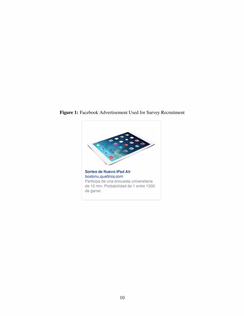
Figure 1: Facebook Advertisement Used for Survey Recruitment

10

Table 2: Online Sample vs. 2012 Census

Sample Sample Census(Used) (Untargeted)

ComunaMedian Population 151,520 152,985 130,808

RegionTarapaca 1.2 1.8 1.7Antofagasta 2.2 2.7 3.2Atacama 1.9 2.1 1.7Coquimbo 3.1 3.7 4.2Araucanıa 5.1 5.2 5.4Metropolitana 36.8 43.1 40.6Valparaıso 15.9 9.9 10.6O’Higgins 3.1 4.2 5.2Maule 4.8 5.7 5.8Biobıo 16.4 11.9 11.9Los Lagos 4.2 3.7 4.7Aysen 0.3 0.1 0.6Magallanes y Antartica 1.5 1.3 1Los Rıos 2.4 2.9 2.2Arica y Parinacota 1.3 1.6 1.3

ReligionCatholic 41.2 41.7 67.4Evangelical 14.8 14.3 16.6Other 4.7 4.2 4.4None 39.4 39.8 11.6

EducationNone 0.2 0.3 2.5Primary 1.4 1.4 25.2Secondary 31.1 31.7 44.2Technical 13.8 14.1 8.9University 51.2 50.8 17.7Postgraduate 2.3 1.8 1.5

OtherMedian Age 21 20 42Male 50.4 51.4 47.9

Individual census figures are for residents 15 and older(religion and education) or 18 and older (other variables).Comuna figures are those associated with the medianindividual. Non-median figures are percentages. Educationis the highest level started or completed. “Used” and“Untargeted” samples are defined in the text.

11

Table 3: Online Sample vs. 2012 AmericasBarometer

Sample Sample Americas(Used) (Untargeted) Barometer

Church Attendance1+ Times/Week 10.6 10.4 7.31 Time/Week 10.7 10.4 12.31 Time/Month 10.7 10.9 19.41–2 Times/Year 20.4 20.5 21.5Never/Almost Never 47.6 47.7 39.4

Party IDNone 78.9 78.8 85.7PS 1.5 1.3 2.9PPD 1.1 1.3 1.5PDC 1.2 1.3 2RN 4.9 4.8 2UDI 3.6 3.8 1.4PC 1.9 1.8 2Other 6.6 6.6 1.2

IdeologyLeft (1–4) 29.1 27.8 34.5Center (5–6) 44.5 44.8 41.8Right (7–10) 26.4 27.4 23.6

All figures expressed as percentages of registered voters.“Used” and “Untargeted” samples are defined in the text.

12

Table 4: Covariate Balance for Pinochet Treatment

Treated Control Std. Diff. Var. Rat. t-test KS-test

ComunaLog Population 11.66 11.71 −0.05 1.04 0.44 0.35

RegionNorth 0.27 0.23 0.08 1.10 0.21Santiago 0.36 0.38 −0.03 0.99 0.70South 0.37 0.39 −0.05 0.98 0.46

ReligionCatholic 0.39 0.44 −0.10 0.96 0.13Evangelical 0.15 0.14 0.04 1.07 0.59Other 0.05 0.04 0.01 1.06 0.83None 0.41 0.37 0.09 1.04 0.20Church Attendance (0–4) 1.14 1.15 −0.01 1.00 0.91 1.00

PoliticsPartisan 0.18 0.23 −0.11 0.85 0.09Ideology (1–10) 5.21 5.35 −0.06 0.95 0.37 0.55Campaign Interest (1–7) 4.37 4.53 −0.08 1.00 0.20 0.40

DemographicsAge 24.06 23.08 0.10 1.43 0.10 0.20Education (1–10) 6.94 6.75 0.11 0.97 0.09 0.04Male 0.52 0.49 0.06 1.00 0.40

NOTE: ‘Treated’ and ‘Control’ give mean values; ‘Std. Diff.’ is their differencedivided by the pooled standard deviation. ‘Var. Rat.’ is the ratio of treatment to controlgroup variance. ‘t-test’ and ‘KS-test’ give two-sided p-values (bootstrapped for KS).

13

Table 5: Covariate Balance for Evangelical Treatment

Treated Control Std. Diff. Var. Rat. t-test KS-test

ComunaLog Population 11.74 11.64 0.09 0.99 0.17 0.22

RegionNorth 0.25 0.25 −0.01 0.99 0.85Santiago 0.36 0.38 −0.05 0.97 0.44South 0.40 0.37 0.06 1.03 0.35

ReligionCatholic 0.39 0.43 −0.07 0.98 0.32Evangelical 0.16 0.14 0.07 1.15 0.30Other 0.05 0.04 0.07 1.39 0.28None 0.39 0.40 −0.02 0.99 0.79Church Attendance (0–4) 1.16 1.14 0.01 1.01 0.84 0.99

PoliticsPartisan 0.20 0.21 −0.04 0.94 0.56Ideology (1–10) 5.34 5.23 0.05 0.99 0.47 0.79Campaign Interest (1–7) 4.56 4.38 0.10 1.01 0.14 0.11

DemographicsAge 23.57 23.64 −0.01 1.01 0.91 0.90Education (1–10) 6.84 6.85 −0.01 0.92 0.91 0.86Male 0.48 0.53 −0.10 1.00 0.15

NOTE: ‘Treated’ and ‘Control’ give mean values; ‘Std. Diff.’ is their differencedivided by the pooled standard deviation. ‘Var. Rat.’ is the ratio of treatment to controlgroup variance. ‘t-test’ and ‘KS-test’ give two-sided p-values (bootstrapped for KS).

14

Table 6: Effect of Pinochet Stereotypes on Vote Intention for an Evangelical Can-didate, by Screener Passage

SubgroupRight-Wing Center-LeftNon-Evangelicals Non-Evangelicals Evangelicals

Intercept 3.58 3.59 5.13(0.56) (0.29) (0.71)

Pinochet Prime 0.69 -0.25 0.43(0.81) (0.4) (0.97)

1 Screener -0.33 -0.59 -0.29(0.79) (0.4) (0.91)

2 Screeners -0.86 -0.89 -0.21(0.7) (0.37) (0.91)

Pinochet × 1 Screener 0.39 -0.18 -0.71(1.27) (0.57) (1.31)

Pinochet × 2 Screeners 0.85 0.49 -1.01(1.01) (0.51) (1.24)

N 82 272 65

NOTE: Entries are OLS regression coefficients with estimated standard errorsin parentheses.

15

Table 7: Effect of Candidate Evangelicalism on Vote Intention When Pinochet Stereo-types Are Not Primed, by Screener Passage

SubgroupRight-Wing Center-LeftNon-Evangelicals Non-Evangelicals Evangelicals

Intercept 4.22 3.48 2.8(0.45) (0.26) (0.57)

Evangelical Candidate -0.64 0.11 2.32(0.71) (0.39) (0.85)

1 Screener -1.14 -0.78 0.37(0.71) (0.4) (0.93)

2 Screeners -0.59 -0.85 0.7(0.62) (0.33) (0.73)

Evang. Cand. × 1 Screener 0.81 0.19 -0.66(1.05) (0.56) (1.24)

Evang. Cand. × 2 Screeners -0.27 -0.04 -0.91(0.92) (0.48) (1.1)

N 95 272 64

NOTE: Entries are OLS regression coefficients with estimated standard errors inparentheses.

16

Table 8: Evangelical Candidates for Deputy Used in the Survey, Chile 2013

Name Party Pact District VotesFrancesca Munoz RN Alianza por Chile 44 (Concepcion) 9.34%Jaime Barrientos UDI Alianza por Chile 13 (Valparaıso) 11.56%Viviana Betancourt PS Nueva Mayorıa 59 (Aisen) 20.91%Jose Aburto PRI PRI 57 (Puerto Montt) 7.27%Susana Garces PRI PRI 58 (Chiloe) 3.12%NOTE: UDI = Independent Democratic Union; RN = National Renewal; PS =Socialist Party; PRI = Regional Party of Independents. None of the candidateswas elected.

17

Table 9: Treatment Effects on Vote Intention for Real vs. FictionalCandidates

Conditional on:Evang. Cand. Pinochet ¬Pinochet

Intercept 3.26 3.46 2.81(0.42) (0.53) (0.43)

Real Candidate -0.08 -0.51 0.97(0.64) (0.68) (0.64)

Pinochet Prime 0.27(0.67)

Real Cand. × Pinochet -0.15(0.9)

Evangelical Candidate 0.07 0.45(0.72) (0.6)

Real Cand. × Evang. Cand. 0.28 -1.05(0.91) (0.9)

N 85 78 79

NOTE: Entries are OLS regression coefficients with estimatedstandard errors in parentheses. Includes only respondents fromcongressional districts with evangelical candidates, as listed inTable 8.

18

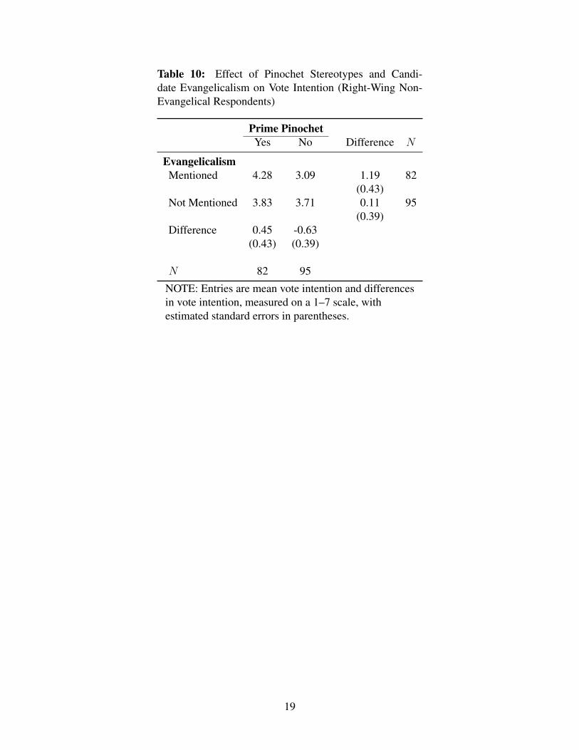
Table 10: Effect of Pinochet Stereotypes and Candi-date Evangelicalism on Vote Intention (Right-Wing Non-Evangelical Respondents)

Prime PinochetYes No Difference N

EvangelicalismMentioned 4.28 3.09 1.19 82

(0.43)Not Mentioned 3.83 3.71 0.11 95

(0.39)Difference 0.45 -0.63

(0.43) (0.39)

N 82 95

NOTE: Entries are mean vote intention and differencesin vote intention, measured on a 1–7 scale, withestimated standard errors in parentheses.

19

Table 11: Effect of Pinochet Stereotypes and CandidateEvangelicalism on Vote Intention (Centrist and Left-WingNon-Evangelical Respondents)

Prime PinochetYes No Difference N

EvangelicalismMentioned 2.96 3.02 -0.06 272

(0.21)Not Mentioned 3.13 2.88 0.25 297

(0.19)Difference -0.16 0.14

(0.2) (0.2)

N 297 272

NOTE: Entries are mean vote intention and differencesin vote intention, measured on a 1–7 scale, withestimated standard errors in parentheses.

20

Table 12: Effect of Pinochet Stereotypes and CandidateEvangelicalism on Vote Intention (Evangelical Respon-dents)

Prime PinochetYes No Difference N

EvangelicalismMentioned 4.73 4.94 -0.21 65

(0.49)Not Mentioned 2.93 3.22 -0.29 59

(0.42)Difference 1.8 1.72

(0.48) (0.44)

N 60 64

NOTE: Entries are mean vote intention and differencesin vote intention, measured on a 1–7 scale, withestimated standard errors in parentheses.

21

Table 13: Effect of Pinochet Stereo-types on Evangelicals’ Vote Intentionfor an Evangelical Candidate, Condi-tional on Ideology

Intercept 4.77(0.78)

Pinochet Prime -1.96(1.07)

Ideology 0.05(0.12)

Pinochet Prime × Ideology 0.33(0.18)

N 64

NOTE: Entries are OLS regressioncoefficients with estimatedstandard errors in parentheses.Ideology is scaled from 1–10;higher numbers are Right.

22

Figure 2: Effect of Pinochet Stereotypes on Evangelicals’ Vote Intention for an Evangelical Can-didate, Conditional on Ideology

2 4 6 8 10

−3

−2

−1

01

23

Ideology

Con

ditio

nal E

ffect

of P

inoc

het P

rime

NOTE: Dotted lines give 95% confidence interval. Plot based on the estimates reported in Table13.

23

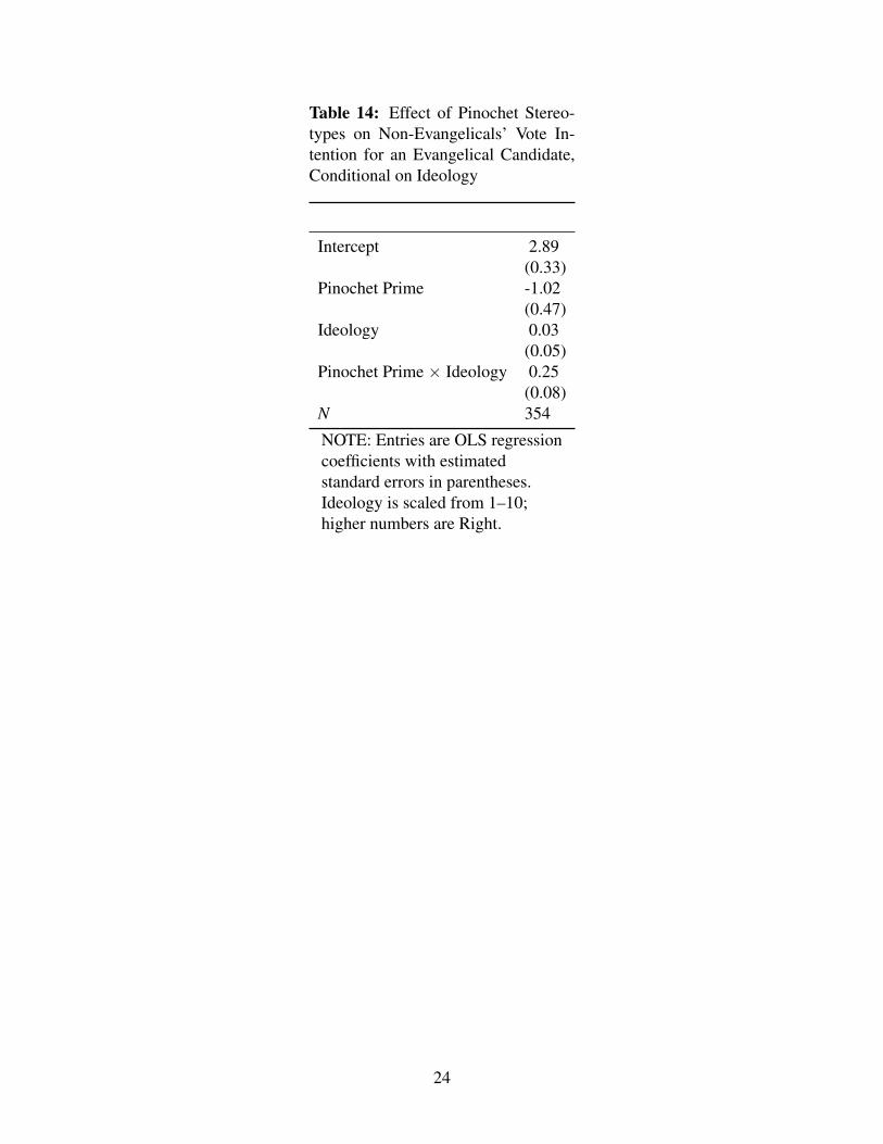
Table 14: Effect of Pinochet Stereo-types on Non-Evangelicals’ Vote In-tention for an Evangelical Candidate,Conditional on Ideology

Intercept 2.89(0.33)

Pinochet Prime -1.02(0.47)

Ideology 0.03(0.05)

Pinochet Prime × Ideology 0.25(0.08)

N 354

NOTE: Entries are OLS regressioncoefficients with estimatedstandard errors in parentheses.Ideology is scaled from 1–10;higher numbers are Right.

24

Figure 3: Effect of Pinochet Stereotypes on Non-Evangelicals’ Vote Intention for an EvangelicalCandidate, Conditional on Ideology

2 4 6 8 10

−1

01

2

Ideology

Con

ditio

nal E

ffect

of P

inoc

het P

rime

NOTE: Dotted lines give 95% confidence interval. Plot based on the estimates reported in Table14.

25

Table 15: Effect of Pinochet Stereotypes onEvangelicals’ Vote Intention for an EvangelicalCandidate, Conditional on Church Attendance

Intercept 2.92(0.59)

Pinochet Prime 1.54(0.92)

Church Attendance 0.82(0.2)

Pinochet Prime × Church Attendance -0.72(0.3)

N 65

NOTE: Entries are OLS regressioncoefficients with estimated standard errors inparentheses. Church Attendance is scaledfrom 0 (never or almost never) to 4 (morethan once a week).

26

Figure 4: Effect of Pinochet Stereotypes on Evangelicals’ Vote Intention for an Evangelical Can-didate, Conditional on Church Attendance

0 1 2 3 4

−3

−2

−1

01

23

Church Attendance

Con

ditio

nal E

ffect

of P

inoc

het P

rime

NOTE: Dotted lines give 95% confidence interval. Plot based on the estimates reported in Table15.

27

Figu

re5:

CO

NSO

RT

Dia

gram

Ass

esse

d fo

r elig

ibili

ty (N

=157

5)

Ran

dom

ized

(N=1

098)

Excl

uded

(N=4

77)

• D

eclin

ed to

par

ticip

ate

(N=5

5)

• D

id n

ot a

nsw

er e

ligib

ility

que

stio

ns (N

=115

) • 

Did

not

mee

t inc

lusi

on c

riter

ia (N

=141

) • 

Qui

t sur

vey

pre-

rand

omiz

atio

n (N

=166

)

Allo

cate

d to

No

Evan

gelic

al/N

o Pi

noch

et in

terv

entio

n (N

=280

) • 

Rec

eive

d in

terv

entio

n (N

=280

)

Allo

cate

d to

No

Evan

gelic

al/

Pino

chet

inte

rven

tion

(N=2

80)

• R

ecei

ved

inte

rven

tion

(N=2

80)

Allo

cate

d to

Eva

ngel

ical

/No

Pino

chet

inte

rven

tion

(N=2

61)

• R

ecei

ved

inte

rven

tion

(N=2

61)

Allo

cate

d to

Eva

ngel

ical

/Pi

noch

et in

terv

entio

n (N

=277

) • 

Rec

eive

d in

terv

entio

n (N

=277

)

Lost

to fo

llow

-up

(N=4

0)

• D

id n

ot a

nsw

er v

ote

ques

tion

(N=2

8)

• D

id n

ot a

nsw

er re

ligio

n qu

estio

n (N

=8)

• N

on-e

vang

elic

al a

nd d

id n

ot

answ

er id

eolo

gy q

uest

ion

(N=4

)

Lost

to fo

llow

-up

(N=3

3)

• D

id n

ot a

nsw

er v

ote

ques

tion

(N=2

3)

• D

id n

ot a

nsw

er re

ligio

n qu

estio

n (N

=8)

• N

on-e

vang

elic

al a

nd d

id n

ot

answ

er id

eolo

gy q

uest

ion

(N=2

)

Lost

to fo

llow

-up

(N=3

7)

• D

id n

ot a

nsw

er v

ote

ques

tion

(N=2

2)

• D

id n

ot a

nsw

er re

ligio

n qu

estio

n (N

=13)

• 

Non

-eva

ngel

ical

and

did

not

an

swer

ideo

logy

que

stio

n (N

=2)

Lost

to fo

llow

-up

(N=3

7)

• D

id n

ot a

nsw

er v

ote

ques

tion

(N=2

6)

• D

id n

ot a

nsw

er re

ligio

n qu

estio

n (N

=9)

• N

on-e

vang

elic

al a

nd d

id n

ot

answ

er id

eolo

gy q

uest

ion

(N=2

)

Ana

lyze

d (N

=223

) • 

Excl

uded

from

ana

lysi

s—re

al c

andi

date

ver

sion

of

inte

rven

tion

(N=1

7)

Ana

lyze

d (N

=228

) • 

Excl

uded

from

ana

lysi

s—re

al c

andi

date

ver

sion

of

inte

rven

tion

(N=1

9)

Ana

lyze

d (N

=208

) • 

Excl

uded

from

ana

lysi

s—re

al c

andi

date

ver

sion

of

inte

rven

tion

(N=1

6)

Ana

lyze

d (N

=211

) • 

Excl

uded

from

ana

lysi

s—re

al c

andi

date

ver

sion

of

inte

rven

tion

(N=2

9)

28

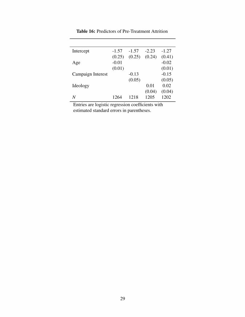
Table 16: Predictors of Pre-Treatment Attrition

Intercept -1.57 -1.57 -2.23 -1.27(0.25) (0.25) (0.24) (0.41)

Age -0.01 -0.02(0.01) (0.01)

Campaign Interest -0.13 -0.15(0.05) (0.05)

Ideology 0.01 0.02(0.04) (0.04)

N 1264 1218 1205 1202

Entries are logistic regression coefficients withestimated standard errors in parentheses.

29

Table 17: Predictors of Post-Treatment Attrition

Intercept -2.51 -2.51 -2.51 -2.31 -2.3 -2.18(0.28) (0.28) (0.27) (0.15) (0.15) (0.48)

Age 0 0(0.01) (0.01)

Campaign Interest -0.06 -0.08(0.05) (0.06)

Ideology 0 0.02(0.05) (0.05)

Pinochet Treatment -0.06 0.02(0.21) (0.22)

Evangelical Treatment -0.02 -0.01(0.21) (0.22)

N 1264 1218 1205 1123 1098 1079

Entries are logistic regression coefficients with estimated standard errorsin parentheses.

30