Particles with spin one - Nikheft45/ftip/Ch04.pdf · number of independent plane-wave solutions of...

4

Particles with spin one

Particles with spin have extra degrees of freedom which transform nontriviallyunder rotations. Such particles are therefore characterized by the value of theirmomentum and by the orientation of their “spin”. For spin-1 this orientationis described by a three-dimensional spin vector. Quantum-mechanically, forgiven momentum, there are three independent states distinguishable by thevalue of the spin projected along a certain axis (in this case these values are ±1and 0 in units of ~). However, massless particles with spin are special, becausetheir spin can only be directed parallel or anti-parallel to their direction ofmotion. Hence, massless particles with spin have only two different spin states,irrespective of the value of their total spin. This chapter deals with spin-1particles, also called vector particles. Well-known examples of massive spin-1particles are the mesons ρ, φ, J/ψ and Υ, and the weak intermediate vectorbosons W± and Z. The only known massless spin-1 particle is the photon.Free massive spin-1 fields are described by the Proca Lagrangian, and masslessspin-1 fields by the Maxwell Lagrangian. We shall discuss four typical particlereactions that involve photons, namely electromagnetic scattering of pions,pion-Compton scattering, the decay π0 → γγ, and the radiative decay K0

S →π+π−γ.

4.1. Massive spin-1 particles

The standard relativistic treatment of spin-1 particles is in terms of a four-vector field Vµ(x), whose free Lagrangian is the Proca Lagrangian,

L = − 14 (∂µVν − ∂νVµ)

2 − 12m

2V 2µ

= − 12 (∂µVν)

2 + 12∂

µVν ∂νVµ − 1

2m2V 2µ . (4.1)

The first and the third term are a straightforward generalization of the Klein-Gordon Lagrangian for scalar fields; the relevance of the second term willbecome clear shortly. The field equations corresponding to (4.1) follow fromHamilton’s principle, according to which we require that the action be sta-tionary under small variations Vµ → Vµ + δVµ, where δVµ, vanishes at theboundary of the integration domain of the action integral. Hence we consider,

δS = −∫

d4x(∂µVν − ∂νVµ

)∂µδV ν +m2Vµ δV

µ(x)= 0 . (4.2)

121

122 Particles with spin one [Ch.4

After integration by parts, using the boundary conditions on δVµ, this reads

δS = −∫

d4x δVµ[Vµ − ∂µ∂νVν −m2V µ

]= 0 , (4.3)

which implies the Proca field equation

(−m2)Vµ − ∂µ∂νVν = 0 . (4.4)

For m2 6= 0 contraction with one more derivative gives ∂µVµ = 0, so that (4.4)is equivalent to the following two equations,

(−m2)Vµ = 0 , ∂µVµ = 0 . (4.5)

The reason for the second term in (4.1) is now clear; its coefficient was chosensuch that one obtains a Klein-Gordon equation for each of the components ofVµ separately, together with a subsidiary restriction. The latter restricts thenumber of independent plane-wave solutions of (4.5) to three, as is appropriatefor a spin-1 particle, i.e.,

Vµ(x) = εµ(k) eik·x , with k2 = −m2) , k · ε(k) = 0 . (4.6)

It is straightforward to define a set of independent polarization vectorsεµ(k). In the rest frame kµ = (0,m), so k · ε(k) = 0 implies that the fourthcomponent of εµ vanishes. In a general frame one distinguishes two differ-ent types of polarizations: two independent transversal polarization vectorswhich are orthogonal to both k and k, and a longitudinal polarization vec-tor whose spatial components are taken along the direction of k. Hence, forkµ = (k, ω(k)), we have two transverse polarizations,

εµ(k;λ) = (ελ, 0) , k · ελ = 0 , (λ = 1, 2) , (4.7)

and one longitudinal polarization,

εµ(k; 0) =(ω(k)km|k| ,−

|k|m

), (4.8)

where we can adopt the convenient normalization

ε(k;λ) · ε(k;λ′) = δλλ′ , λ , λ′ = 1, 2, 0 . (4.9)

Note that the distinction between transversal and longitudinal polarizationvectors is not a Lorentz invariant notion, since transversal and longitudinalpolarization vectors rotate into each other by a Lorentz transformation.

We have assumed above that the polarization vectors are real ((εµ = εµ).The corresponding plane waves (4.6) are then linearly polarized. Another

§4.1] Massive spin-1 particles 123

choice for the polarization vectors, which is often convenient, involves helic-ity eigenvectors. Helicity measures the spin of the particle along its directionof motion (in units of ~). To measure the spin along k one applies a rota-tion around k to the field. For k pointing in the positive z-direction such a(clockwise) rotation takes the form

Vµ(k)→ V ′µ(k) = Lµν Vν(k) ,

with

Lµν =

cos θ sin θ

− sin θ cos θ

1

1

. (4.10)

A polarization vector with helicity λ is an eigenstate of the rotation matrixwith eigenvalue exp(iλθ). Obviously, the longitudinal polarization vector (4.8)is invariant under the rotation, and has thus zero helicity. The transversepolarization vectors (4.7) now decompose into two helicity eigenvectors withλ = ±1, which are complex, namely (with k in the positive z-direction),

εµ(k;±) = 12

√2(1 ,±i , 0 , 0) (4.11)

while the zero-helicity vector is the longitudinal one given by (4.8). The po-larization vectors (4.8) and (4.11) characterize incoming particles of corre-sponding helicities. For outgoing particles one must use the conjugate vectorspolarization vectors ε(k;λ). For complex polarization vectors we have the(Lorentz invariant) orthonormality conditions,

ε(k, λ) · ε(k, λ′) = δλλ′ , (λ, λ′ = +,−, 0) (4.12)

corresponding to (4.9).Let us now turn to the Feynman rules. For vector fields the construction of

Feynman diagrams proceeds along the same lines as for scalar fields. Becausea vector field consists of four separate components, the propagator takes theform of a 4 × 4 matrix. Its derivation follows directly from the prescriptiongiven in section 2.4. First we construct the Fourier transform of the actioncorresponding to (4.1)

S[Vµ] = − 12 (2π)

4

∫d4k Vµ(k)

[(k2 +m2)ηµν − kµkν

]Vν(k) , (4.13)

where Vµ(k) = Vµ(−k) because Vµ(x) is a real field. The propagator is theinverse of the matrix in the integrand, viz.

∆µν(k) =1

i(2π)2[(k2 +m2)ηµν − kµkν

]−1. (4.14)


In order to calculate the inverse of this matrix it is convenient to first decom-pose ∆µν according to ∆µν(k) = A(k2)ηµν+B(k2)kµkν , after which one findsA(k2) and B(k2) by requiring that

i(2π)4∆µν(k) [(k2 +m2)ηνρ − kνkρ] = δµ

ρ .

The result is

∆µν(k) =1

i(2π)41

k2 +m2

(ηµν +

kµkνm2

). (4.15)

As we have been emphasizing in chapter 2 the propagator poles at k2 = −m2

are associated with physical particles. Therefore, at first sight, it may seemthat (4.15) describes four rather than three physical degrees of freedom withmassm, because of the overall factor (k2+m2)−1. However, this is no the case.The three polarization vectors (4.8) and (4.8) have zero innder product withkµ, and are thus eigenvectors of (4.15) with equal eigenvalues proportionalto (k2 + m2)−1. The remaining eigenvector is proportional to kµ, and itseigenvalue has no pole at k2 = −m2. Indeed, one easily verifies that

∆µν(k)kν =

kµi(2π)4m2

. (4.16)

Figure 4.1: Graphical representation of the propagator ∆µν(k).

The endpoints of the propagator lines carry a four-vector index, as is indi-cated in fig. 4.1. To define the probability amplitude one follows the prescrip-tion given in section 3.3. This leads to a residue matrix (ηµν +m−2kµkν) forevery external line. However, physical particles are characterized by polariza-tion vectors εµ that are orthogonal to kµ, so that the kµkν term drops out.On the other hand, it is not really necessary to impose (??) as an independentrestriction; on the mass shell (k2 = −m2) the polarization vector εµ ∝ kµ,does not contribute by virtue of (4.16). By the same arguments wave functionsare decomposed as (cf. (3.3),

fµ(x) =1

(2π)3/2

∫d3k√2ω(k)

3∑

λ=1

f (λ)(k) εµ(k, λ) eik·x−iω(k)t ,

§4.2] Massive spin-1 particles 125

where one includes only the physical polarization vectors.The invariant amplitude for a process involving n vector particles charac-

terized by polarization vectors εµ(k, λ) takes the form

Mλ1···λn =Mµ1···µn εµ1(k1;λ1) · · · εµn

(kn;λn) , (4.17)

where we have now dropped the kµkν-terms of the propagator residues for theexternal lines. In the definition of the probability amplitude one now encoun-ters the same normalization factors [(2π)32ω(k)]−1/2 as for scalar particles.The transition probability for a given process is proportional to the square ofthe invariant amplitude. When the details of the final state are not of interestone sums over all possible spin orientations of the outgoing particles. Fur-thermore, as particle beams are often unpolarized, the spin of the incomingparticles may be unknown, so one averages over all the possible spins of theincoming particles. Let us consider just one of the polarization vectors in theinvariant amplitude in order to show how the summation over spins is done.Hence we write

Mλ =Mµ εµ(k;λ) . (4.18)

Remember that the spin of incoming particles is characterized by εµ(k, λ),while for outgoing particles one must take the conjugate vector εµ(k, λ). Thesquare of (4.18) is

|Mλ|2 =∑

µ,ν

εµ(k, λ) εν(k;λ)Mµ Mν (4.19)

Summing (4.19) over λ gives

∑

µ,ν

(∑

λ

εµ(k;λ) εν(k;λ))Mµ Mν . (4.20)

One way to evaluate the polarization sum makes use of explicit expressionsfor the polarization vectors. For orthonormal vectors one always finds,

∑

λ

εµ(k;λ) εν(k;λ) = ηµν +kµkνm2

. (4.21)

This result does not come as a surprise, because the vectors εµ(k;λ) spanthe three-dimensional subspace that is orthogonal to the vector kµ with k2 =−m2; indeed, multiplying the right-hand side of (4.21) with kµ gives zero onthe mass-shell.


4.2. Massless spin-1 particles

One might expect that the description of massless spin-1 particles shouldfollow directly from the theory of massive spin-1 particles, but we shall seethat this not the case. This is for instance obvious from the fact that theexpression for the longitudinal polarization vector (4.8) and the propagator(4.15) are singular in the limit m → 0. A primary reason for this is that themassless limit of (4.1),

L = − 14 (∂µAν − ∂νAµ)

2 , (4.22)

is invariant under local gauge transformations

Aµ(x)→ Aµ(x) + ∂µξ(x). (4.23)

This transformation is familiar from Maxwell’s theory of electromagnetismwhere the vector potential is subject to the same transformations (see sec-tion 1.3). Therefore we have changed notation in this section and denote themassless vector field by Aµ. The electromagnetic field strength equals

Fµν = ∂µAν − ∂νAµ , (4.24)

and the particles described by this theory are called photons.One consequence of an invariance under local gauge transformations is that

the theory depends on a smaller number of fields. Correspondingly the numberof plane wave solutions is also reduced in comparison to the massive case. Tosee this explicitly, consider the field equation following from (4.22) and inves-tigate its possible plane-wave solutions. The field equation is just Maxwell’sequation,

∂ν(∂νAµ − ∂µAν) = 0 . (4.25)

In order to examine plane-wave solutions of this equation we consider theFourier transform of Aµ(x)

Aµ(k) = (2π)−4∫

d4xAµ(x) e−ik·x . (4.26)

Under gauge transformations Aµ(k) changes by a vector proportional to kµ

Aµ(k)→ A′µ(k) = Aµ(k) + ξ(k) kµ . (4.27)

The field equation (4.25) now takes the form

k2Aµ(k)− kµkνAν(k) = 0 , (4.28)

§4.2] Massless spin-1 particles 127

which is manifestly invariant under the transformation (4.27). DecomposingAµ(k) into four independent vectors, εµ(k, λ), kµ and kµ, defined by

kµεµ(k;λ) = 0 , ε0(k;λ) = 0 , (λ = 1, 2) ,

kµ = (k, k0) , kµ = (k,−k0) , (4.29)

we decompose,

Aµ(k) = aλ(k) εµ(k, λ) + b(k) kµ + c(k) kµ . (4.30)

The field equation (4.28) now corresponds to

k2aλ(k) εµ(k, λ) + b(k) [k2 kµ − (k · k) kµ] = 0 , (4.31)

from which we infer for the coefficient functions (note that k · k is positive),

k2aλ(k) = 0 , (λ = 1, 2) b(k) = 0 . (4.32)

Obviously the field equation does not lead to any restriction on c(k). Thisshould not come as a surprise because c(k) can be changed arbitrarily by agauge transformation, whereas the field equation is gauge invariant. Conse-quently the field equation cannot fix the value of c(k). By means of a gaugetransformation we may adjust c(k) to zero, which shows that c(k) has no phys-ical meaning. We thus find that there are only two independent plane wavesolutions characterized by lightlike momenta (k2 = 0) and the two transversepolarization vectors.The fact that we have two rather than three solutions indicates that a direct

generalization of the arguments of the previous section runs into difficulties.One such difficulty is that the spin of a massless particle cannot be definedby referring to its rest frame. Therefore, the three-dimensional rotation groupno longer plays the decisive role in order to characterize the spin, but ratherthe group of two-dimensional rotations around the three-momentum k of theparticle. This complication is also apparent from the singular dependenceof the longitudinal polarization vector (4.8) on the mass. One may wonderwhether a characterization of the spin in terms of only transverse polarizationswill not lead to a violation of Lorentz invariance in view of the fact thattransversality is not preserved by Lorentz transformations. However, it turnsout that Lorentz invariance is preserved provided that the photon field couplesto a conserved current (i.e. ∂µJ

µ = 0). As is well-known from electrodynamicsthis is indeed the case (see, again, section 1.3. Conserved currents can beviewed as a consequence of gauge invariance.There is a further difficulty when attempting to calculate Feynman diagrams

for massless spin-1 particles, again related to the aforementioned invariance


under gauge transformations. To show this consider the Fourier transform ofthe action corresponding to (21.34), viz.

S[Aµ] = − 12 (2π)

4

∫d4k Aµ(k)

[k2ηµν − kµkν

]Aν(k) . (4.33)

According to the general prescription the propagator is proportional to theinverse of [k2ηµν − kµkν ]. In this case, however, the inverse does not existbecause the matrix has null vector, as we see from

[k2ηµν − kµkν

]kν = 0 . (4.34)

The existence of the null vector is a direct consequence of the gauge invarianceof the theory. Gauge invariance implies that the theory contains fewer degreesof freedom; this fact must reflect itself in the presence of zero eigenvalues inthe quadratic part of the Lagrangian. Indeed, the null vector proportional tokµ is directly associated with the gauge transformation (4.27) in momentumspace. Obviously, the degree of freedom that is absent in (4.33) should notreappear through the interactions. One can show that this is ensured providedthat the photon couples to a conserved current (see problem 4.5).

The standard way to circumvent the singular propagator problem is to makeuse of a gauge condition. A convenient procedure is based on introducing themissing (gauge) degrees of freedom, which formally spoils the gauge invariance.However, the degrees of freedom are introduced only in order to make thepropagator well-defined and they will not affect the interactions of the theory.Therefore, the effect of this procedure can still be separated from the truegauge invariant part of the theory, and the physical consequences remainunchanged. It is a rather subtle matter to prove that this is indeed the case.In this section we only present the prescription for defining the propagator.To do that one introduces a so-called “gauge-fixing” term to the Lagrangian.The most convenient choice is to add to (4.22)

Lg.f. = − 12 (λ∂

µAµ)2 , (4.35)

where λ is an arbitrary parameter. Because of this term the Fourier transformof the action corresponding to the combined Lagrangian becomes

S[Aµ] = − 12 (2π)

4

∫d4k Aµ(k)

[k2ηµν − kµkν + λ2kµkν

]Aν(k) , (4.36)

so that for λ 6= 0 the propagator is equal to

∆µν(k) =1

i(2π)4[k2ηµν − (1− λ2)kµkν

]−1

=1

i(2π)41

k2

(ηµν − (1− λ−2)kµkν

k2

). (4.37)

§4.3] Electromagnetic scattering of pions 129

Clearly the propagator has more poles at k2 = 0 than there are physical pho-tons (characterized by transversal polarizations). However, one must realizethat by making the above modification we have somewhat obscured the re-lation between propagator poles and physical particles. In order to extractthe physical content of the theory one should contract the amplitude withonly transversal polarization vectors. This requirement forms an essential in-gredient of the proof that physical results do not depend on the parameterλ.Using the propagator (4.37) one can now construct Feynman diagrams and

corresponding scattering and decay amplitudes for photons in the standardfashion. The λ-dependent kµkν-term of the propagator residue vanishes whencontracting the invariant amplitude with transversal polarization vectors. Inorder to sum over photon polarizations one may use (for orthonormal polar-ization vectors)

∑

λ=1,2

εµ(k;λ) εν(k;λ) = ηµν −kµkν + kµkν

k · k, (k2 = 0) , (4.38)

where the vector kµ was defined in (4.29). In order to verify this equation wenote that the right-hand side of (4.38) is equal to

∑

λ=1,2

εµ(k;λ) εν(k;λ) =

ηµν −kµkν|k|2 for µ, ν = 1, 2, 3;

0 for µ and/or ν = 0.(4.39)

Obviously (4.38)-(4.39) are not manifestly Lorentz covariant, which is relatedto the fact that the transversality condition k · ε(k, λ) = 0 is not Lorentzinvariant. However, if the photons couple to conserved currents, such that theamplitude vanishes when contracted with the photon momentum,

kµMµ = 0, (4.40)

then the non-covariant terms in (4.38) may be dropped. Consequently, whensumming |Mµεµ(k;λ)|2 over the transverse polarizations, one has

∑

λ=1,2

|Mµ εµ(k;λ)|2 =MµMµ , (4.41)

which is manifestly Lorentz invariant.

4.3. Electromagnetic scattering of pions

In order to illustrate the use of Feynman diagrams for spin-1 particles considerthe reaction caused by virtual photon exchange. This π+π− → π+π− process


is not of direct physical relevance. Pion targets or colliding pion beams are notavailable, and even if they were it would be almost impossible to distinguishthe electromagnetic contributions to this scattering process from those of thestrong interactions, which are dominated by ρ-meson exchange. Nevertheless itis of interest to give the relevant expression for pure electromagnetic scatteringof pointlike spinless particles, in order to appreciate the more complicated butanalogous results for the scattering of pointlike spin- 12 fermions. The latterwill be discussed extensively in chapter 6..The pion-photon coupling follows from the minimal substitution ∂µφ →

∂µφ − ieAµφ in the free Klein-Gordon Lagrangian, where (φ is a complexscalar field (e is the π+ charge). Combining this with Maxwell’s Lagrangiangives

L = − 14FµνF

µν − ∂µφ∗∂µφ−m2φ∗φ

− ieAµ[φ∗(∂µφ)− (∂µφ∗)φ]− e2A2

µ φ∗φ . (4.42)

The electromagnetic couplings are the same as used in section 2.3 to studythe scattering of pions by an external electromagnetic potential. An importantproperty of the Lagrangian (4.42), is its invariance under the combined gaugetransformations

Aµ(x)→ Aµ(x) + ∂µξ(x) , φ(x)→ eieξ(x)φ(x) . (4.43)

The propagators and vertices implied by (4.42) are shown in table 4.1. Thearrow on the pion line indicates the flow of (positive) charge rather than of themomentum. Just as in section 2.3 we choose conventions such that an outgoingarrow on an external line indicates the emission of a π+ or the absorption ofa π−.

Table 4.1: Feynman rules corresponding to the Lagrangian (4.45)a.

Two diagrams contribute in lowest order to the amplitude for π+π− →π+π−. They are given in fig. 4.2 where the momentum assignments are de-fined. We distinguish a scattering and an annihilation diagram, which arerelated by an interchange of the momenta (p2 → −q1). Note that p1, p2, q1and q2 denote the particle momenta, so that the momentum flow and thecharge flow in the diagrams do not always coincide. As usual we extract anoverall factor of i(2π)4 and a momentum-conserving δ-function. The invariant


Figure 4.2: Tree diagrams contributing to the electromagnetic scattering ofcharged pions.

amplitude is given by

M =e2(p1 + p2)

µ(−q1 − q2)ν(p1 − p2)2

[ηµν − (1− λ−2) (p1 − p2)µ(q2 − q1)ν

(p1 − p2)2]

+e2(p1 − q1)µ(p2 − q2)ν

(p1 + q1)2

[ηµν − (1− λ−2) (p1 + q1)µ(p2 + q2)ν

(p1 + q1)2

],

(4.44)

where we have set the photon momentum equal to kµ = (p1−p2)µ = (q2−q1)µin the scattering diagram, and to kµ = (p1+q1)

µ = (p2+q1)µ in the annihila-

tion diagram. A first important observation is that the gauge-dependent partof the photon propagator vanishes when the pions are taken on the mass shell,because (p1+p2) ·(p1−p2) = p21−p22 = 0 and (p1−q1) ·(p1+q1) = p21−q21 = 0.This confirms that the physical consequences of the theory have not been af-fected by introducing the gauge-fixing term (4.35) into the Lagrangian.Introducing Mandelstam variables

s = −(p1 + q1)2 , t = −(p1 − p2)2 , u = −(p1 − q2)2 ,

the amplitude can be written in a simple form

M = e2(u− s

t+u− ts

). (4.45)

This result remains relevant when the four external particles are not allof the same type. For instance, if we assume that π+ and π− are not each


others antiparticle, but unrelated positively and negatively charged particles ofdifferent mass, then the annihilation diagram is not possible and the scatteringdiagram gives

Mscatt = e2u− st

. (4.46)

On the other hand, if the incoming and outgoing particles are of different type,then the scattering diagram is not possible and the annihilation diagram gives

Mann = e2u− ts

. (4.47)

The above results allow us to discuss a few typical reactions. First considerthe case described by (4.45), which in the analogous case of electron-positronscattering is called Bhabha scattering. In the centre-of-mass frame t and u areexpressed in terms of s and the scattering angle θ between p1 and p2

t = −(s− 4m2) sin2 12θCM ,

u = −(s− 4m2) cos2 12θCM . (4.48)

The differential cross section follows directly from (3.51)

dσ

dΩCM=

α2

4s31

sin4 12θCM

s2

s− 4m2+ s(1− 2 sin2 1

2θCM + 2 sin4 12θCM)

+4m2 sin2 12θCM(1− 2 sin2 1

2θCM)2

, (4.49)

where α is the fine-structure constant (αs = e2/4π). Obviously the complexityof this expression is caused by the fact that there are two diagrams involved.At high energy (4.49) simplifies to

dσ

dΩCM=α2

s

(1− sin2 12θCM + sin4 1

2θCM)2

sin4 12θCM

. (4.50)

If there is only one diagram then the result is much simpler. For instance,if we have a pure annihilation reaction, say of π+π− into another chargedparticle-antiparticle pair (with mass M), the cross-section reads (using 4.47)

dσ

dΩCM=α2

4s

(s− 4m2

s

)1/2(s− 4M2

s

)3/2cos2 θCM , (4.51)

or, for s≫ m2,M2,

dσ

dΩCM=α2

4scos2 θCM . (4.52)


The scattering amplitude for π− scattering off some positively charged particlewith massM follows from (4.46). Substituting this result into (3.55) we obtain

dσ

dt= πα2

s

(u− st

)2λ−1(s,M2,m2) . (4.53)

Let us convert (4.53) into the laboratory frame, where the energies of theincoming and outgoing pions are E and E′, respectively, and the outgoingpion is deflected over an angle θ. After the scattering has taken place thetarget particle is no longer at rest and has an energy ER (cf. 3.56). A generalformula for the differential cross section in the laboratory system is given in(3.60). If we assume that the pion mass may be neglected it is easy to expressE′ in terms of θ. Using t = −2EE′(1− cos θ) = 2M(M −ER) = 2M(E′ −E)we find

E′ =E

1 + 2E/M sin2 12θ

,

t =−4E2 sin2 1

2θ

1 + 2E/M sin2 12θ

,

s = M2 + 2ME ,

u = M2 − 2ME − t . (4.54)

Combining (3.60), (4.53) and (4.54) then leads to

dσ

dΩlab=

α2s

4E2 sin4 12θ

( 1 + E/M sin2 12θ

1 + 2E/M sin2 12θ

)2. (4.55)

In the limit that M →∞ we obtain the celebrated Rutherford cross section.The extra factor on the right-hand side of (4.55) represents the recoil correc-tion for the target particle. As we shall see in chapter 6 such recoil correctionsdepend on the spin of the target particle.The observant reader should have noticed that the differential cross sections

(4.49) and (4.55) diverge in the forward direction (i.e. t or θ → 0). Twocomments will help to clarify this phenomenon. One is that a differential crosssection can never be measured at θ = 0 as the scattered particles cannot beseparated from the unscattered beam. Hence measurements of the differentialcross sections are made in a flnite range of θ > 0. The second comment istheoretical. Since the range of the electromagnetic interaction is infinite, softphotons will always be radiated in the collisions of charged particles. Thereforehigher-order corrections must be taken into account before it is possible todefine a total cross section. In section 4.6 we shall discuss a similar problemin the definition of the decay rate for K0

S → π−π+γ.


4.4. Pion-Compton scattering

A reaction that involves real photons is pion-Compton scattering, i.e. γ(k) +π+(p)→ γ(k′) + π+(p′), where the particle momenta are indicated in paren-theses. Information on this reaction has been obtained from a study of piondissociation in the Coulomb field of a heavy nucleus (i.e. π+ + nucleus →π+ + γ + nucleus). However, for our immediate purpose the experimental as-pects are not terribly relevant, and we can always take a limit of low-energyphoton scattering, in which the spin of the target plays no role, and therebysingle out nonrelativistic Compton scattering, a process for which there isadequate experimental data. First some kinematics: in the laboratory frame,with m the pion mass, ω, ω′ the incoming and outgoing photon energies,respectively, and θ the scattering angle, we can write the four momenta as

p = m(0, 0, 0, i) ,

k = ω(0, 0, 1, i) ,

k′ = ω′(sin θ, 0, cos θ, i) ,

p′ = (−ω′ sin θ, 0, ω − ω′ cos θ, i(m+ ω − ω′)). (4.56)

Energy momentum conservation tells us that (p+k)2 = (p′+k′)2 or p·k = p′·k′leading to the famous relation

ω′ =ω

1 + ω/m(1− cos θ), (4.57)

which coincides with the first equation in (4.54). Hence the two-particle kine-matics does not allow us to let ω′ → 0 without ω → 0 at the same time. Forlater use we list the Mandelstam variables (which may again be compared toresults in (4.54))

s = (p+ k)2 = m2 + 2mω ,

t = −(k − k′)2 = −2ωω′(1− cos θ) =−2ω2(1− cos θ)

1 + ω/m(1− cos θ). (4.58)

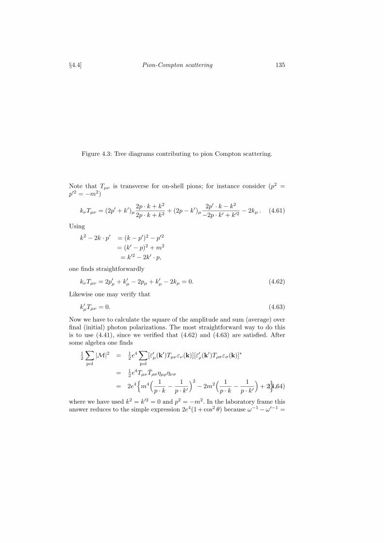
The lowest-order diagrams for pion-Compton scattering follow from the La-grangian (4.42). There are three diagrams shown in fig. 4.3. The third diagramrequires a combinatorial factor of 2 to account for the two possible ways ofattaching the photon lines. The corresponding invariant amplitude contractedwith the photon polarization vectors ε(k′) and ε(k) is

M = e2ε′µ(k′)Tµν(k

′, k)εν(k) , (4.59)

with

Tµν =(2p′ + k′)µ(2p+ k)ν

(p+ k)2 +m2+

(2p− k′)µ(2p′ − k)ν(p− k′)2 +m2

− 2ηµν . (4.60)

§4.4] Pion-Compton scattering 135

Figure 4.3: Tree diagrams contributing to pion Compton scattering.

Note that Tµν is transverse for on-shell pions; for instance consider (p2 =p′2 = −m2)

kνTµν = (2p′ + k′)µ2p · k + k2

2p · k + k2+ (2p− k′)µ

2p′ · k − k2−2p · k′ + k′2

− 2kµ . (4.61)

Using

k2 − 2k · p′ = (k − p′)2 − p′2= (k′ − p)2 +m2

= k′2 − 2k′ · p,one finds straightforwardly

kνTµν = 2p′µ + k′µ − 2pµ + k′µ − 2kµ = 0. (4.62)

Likewise one may verify that

k′µTµν = 0. (4.63)

Now we have to calculate the square of the amplitude and sum (average) overfinal (initial) photon polarizations. The most straightforward way to do thisis to use (4.41), since we verified that (4.62) and (4.63) are satisfied. Aftersome algebra one finds

12

∑

pol

|M|2 = 12e

4∑

pol

[ε′µ(k′)Tµνεν(k)][ε

′ρ(k′)Tρσεσ(k)]

∗

= 12e

4Tµν Tρσηµρηνσ

= 2e4m4( 1

p · k −1

p · k′)2− 2m2

( 1

p · k −1

p · k′)+ 2,(4.64)

where we have used k2 = k′2 = 0 and p2 = −m2. In the laboratory frame thisanswer reduces to the simple expression 2e4(1+cos2 θ) because ω−1−ω′−1 =


−m−1(1 − cos θ). Although at first sight the formulae in (4.60) and (4.64)seem to diverge as ω or ω′ → 0, the answer thus remains finite (infinitiesthat usually arise in this limit are called infrared divergences). The absenceof the divergence can be understood from the fact that the virtual pion in thefirst two diagrams of fig. 4.3 cannot approach its mass shell without violatingangular momentum conservation.Now that we have the result above, we should comment that there is a

faster way to do the calculation. Begin in the laboratory frame and choosethe following set of independent real polarization vectors

εµ(k, 1) = (1, 0, 0, 0) ,

εµ(k, 2) = (0, 1, 0, 0) ,

ε′µ(k′, 1) = (− cos θ, 0, sin θ, 0) ,

ε′µ(k′, 2) = (0, 1, 0, 0) , (4.65)

which satisfy p · ε = p · ε′ = k · ε = k′ · ε′ = 0. Therefore the amplitude (4.59)reduces to M = −2e2ε(k) · ε′(k′). If we then perform the explicit sum overthe (real) polarization vectors (4.65) the result is

12

∑

pol

|M|2 = 2e4∑

λ,λ′=1,2

εµ(k, λ)ε′µ(k′, λ′)ερ(k, λ)ε

′ρ(k′, λ′)

= 2e4(1 + cos2 θ) . (4.66)

The differential cross section in the laboratory frame follows from (3.55),

dσ

dt=

1

16π

1

(s−m2)2

(12

∑

pol

|M|2), (4.67)

and (3.60), which reduces to

dσ

dΩlab=ω′2

π

dσ

dt(4.68)

Comparing the above formulae one finds

dσ

dΩlab=

α2

2m2

1 + cos2 θ

(1 + ω/m(1− cos θ))2, (4.69)

where α is the fine-structure constant. In the limit ω → 0 we may compare(4.69) to the result for scattering of classical electromagnetic radiation

dσ

dΩlab=

α2

2m2(1 + cos2 θ) . (4.70)

The corresponding total cross section,

σ =8πα2

3m2, (4.71)

§4.5] Decay rate for π0 → γγ 137

is named after Thomson, and provides a means to measure the ratio of thecharge to the mass of a particle. In units where ~ = c = 1, 1 GeV−2 = 389µbso the cross section is 8.8µb. For photon-electron scattering the Thomson crosssection is much larger, since one replaces m by the (much smaller) electronmass. The cross section for radiation on an atomic electron is equal to 0.66 b.

4.5. Decay rate for π0 → γγ

The lifetime of the neutral pion is τπ0 = 0.83 × 10−16 s. The particle decaysprimarily into two photons, and has small branching ratios into the modese+e−γ and e+e−e+e−. In this section we calculate the decay rate for π0 → γγstarting from the interaction Lagrangian

Lint = iαCεµνρσFµνFρσφ. (4.72)

In (4.72) C is a coupling constant with dimension [mass]−1, α is the fine-structure constant (α = e2/4π), Fµν is the field-strength tensor defined in(4.24), and φ is the field associated with the neutral pion (εµνρσ is a completelyantisymmetric tensor normalized such that ε1234 = 1). We should point outthat the Lagrangian (4.72) is only introduced here as a useful mnemonic forwriting down the amplitude, without pretending that it describes some fun-damental theory. In this context one often uses the term “phenomenological”or “effective” Lagrangian. If the photons and the pion are on their respectivemass shells C is just a constant, because all Lorentz-invariant combinationsof the external momenta in a three-point vertex can be expressed in termsof the masses of the incoming and outgoing particles. Therefore, taking thelowest-order diagram corresponding to (4.72) will describe the full result forπ0 → γγ in terms of an unknown parameter C. We shall argue later that itis possible to construct models in which one can calculate C.

The effective Lagrangian (4.72) can be motivated as follows. Since the La-grangian must be gauge invariant the photon field must be expressed in termsof the gauge-invariant tensor Fµν (we have two tensors Fµν because we needa three-point vertex with two photon fields and one pion field). The fine-structure constant has been introduced since we expect that each photon cou-ples with a strength proportional to the elementary charge e. The pion hasnegative intrinsic parity which means that the field φ changes under parityaccording to

φ(x, t)P→φp(x, t) = −φ(−x, t). (4.73)

Under parity reversal Fµν transforms as

Fµν(x, t)P→F pµν(x, t) =

−Fµν(−x, t) if µ or ν = 0 ,+Fµν(−x, t) if µ or ν 6= 0 .

(4.74)


Figure 4.4: Diagram describing the decay π0 → γγ.

Therefore we have introduced the ε-tensor because εµνρσFµνFρσ has negativeintrinsic parity. This can be seen more easily by expressing Fµν in terms ofthe magnetic and electric fields; εµνρσFµνFρσ is proportional to E · B, andas is well-known E transforms as a vector and B as an axial vector underx → −x. Because the ε-symbol forces precisely one of the indices µ, ν, ρ orσ to be equal to 4, and Fµ4 is imaginary in our convention, εµνρσFµνFρσ ispurely imaginary. Therefore we have introduced a factor i in (4.72) so that Cis real.In order to calculate the decay rate for π0(Q)→ γ(p) + γ(q) we must first

find the invariant amplitude which corresponds to the diagram in fig. 4.4.After contraction with transverse polarization vectors ε1(p) and ε2(q) for theoutgoing photons we have

M(π0 → γγ) = 2iαCεµνρσ(−2ipµε1ν(p))(−2iqρε2σ(q)) , (4.75)

where the overall factor of 2 arises because the external photons can be hookedto the vertex in two different ways. The terms −2ipµε1ν(p) and −2iqρε2σ(q)arise from each of the field strength tensors, where we have defined the mo-menta of the photons as outgoing; the factor of two in both expressions orig-inates from the fact that Fµν contains two terms (cf. 4.24) which add as aresult of the antisymmetry of the ε-symbol.To calculate the decay rate one must first square the amplitude (4.40):

|M(π0 → γγ)|2 = (8αC)2|εµνρσpµqρε1ν(p)ε2σ(q)|2 . (4.76)

We first note that εµνρσpµqρε1ν(p)ε2σ(q) is purely imaginary because the ε-symbol forces precisely one of the indices to be equal to 4. Therefore we maywrite

|εµνρσpµqρε1ν(p)ε2σ(q)|2 =

= −εµνρσεµ′ν′ρ′σ′pµqρpµ′qρ′ ε1ν(p)ε1ν′(p)ε2σ(q)ε2σ′(q) . (4.77)


Now we recall the following property of the ε-symbol:

εµνρσεµ′ν′ρ′σ′ =∑

perm

(−1)P ηµµ′ηνν′ηρρ′ησσ′ , (4.78)

where we sum over all 24 permutations of the indices µ, ν, ρ, σ, and (−)P isminus (plus) if the permutation is odd (even). Equation (4.78) is based on theobservation that the set of indices [µνρσ] as well as [µ′ν′ρ′σ′] must cover allindex values in some permutation, so that each of the [µνρσ] should coincidewith precisely one of the [µ′ν′ρ′σ′] indices (see appendix B).

Only 5 permutations in (4.78) contribute, because of the relations k2 =k · ε = 0 for photons. The result can thus be cast in the form

|M(π0 → γγ)|2 = (8αC)2 14m4π[(ε1(p) · ε1(p))(ε2(q) · ε2(q))− |ε1(p) · ε2(q)|2]

− 12m

2π[(Q · ε1(p))(Q · ε2(q))(ε1(p) · ε2(q))

+(Q · ε1(p))(Q · ε2(q))(ε1(p) · ε2(q))]+|Q · ε1(p)|2|Q · ε2(q)|2 , (4.79)

where Qµ is the π0 momentum and we have used

p · ε2(q) = Q · ε2(q) ,q · ε1(p) = Q · ε1(p) ,

p · q = 12Q

2 − 12p

2 − 12q

2 = 12m

2π . (4.80)

If we consider (4.79) in the rest frame, where Q · ε1(p) = Q · ε2(q) = 0,we find that |M|2 is proportional to ((ε1 · ε1)(ε2 · ε2) − |ε1 · ε2|2). This maybe compared to the analogous result for the two-photon decay of a scalarmeson, since an even-parity interaction φFµνFµν leads to |M|2 proportional to|ε1 ·ε2|2. Conservation of angular momentum implies that two spin-1 particlesproduced by the decay of a spinless particle should have equal helicities inthe rest frame of this particle (see fig. 4.5). Equal helicity means that ε1 = ε2(as the spin-1 particles move in opposite directions), opposite helicity impliesε1 = ε2. Since helicity vectors satisfy ε · ε = 1 and ε · ε = 0 (cf. 4.11a) onereadily verifies that both ((ε1 · ε1)(ε2 · ε2) − |ε1 · ε2|2) and |ε1 · ε2|2 vanishfor ε1 = ε2, and are equal to unity for ε1 = ε2. Consequently the restrictionsimposed by angular momentum conservation are satisfied in both cases.

However, one may also analyze the decay in terms of linear photon polar-izations (ε = ε, as shown by 4.8a). In that case one readily concludes that(ε1 · ε1)(ε2 · ε2) − |ε1 · ε2|2) vanishes if the plane polarizations of the twophotons are parallel, whereas |ε1 · ε2|2. vanishes if the plane polarizations areperpendicular. In principle this feature can be used to determine the intrin-sic parity of the decaying spinless particle. For example, if the photon werean unstable particle, its two-body decay would define a plane whose orienta-tion would be correlated to the polarization of the photon. If both photons


Figure 4.5: Photon helicities in the rest frame of the decaying π0. Oppositehelicity photons are forbidden by angular momentum conservation.

decayed one could thus measure the number of events as a function of theangle θ between the two decay planes. For pseudoscalar mesons one expectsa sin2 θ = 1

2 (1 − cos 2θ) distribution whereas scalar mesons give rise to acos2 θ = 1

2 (1 + cos 2θ) distribution. The photon, however, is a stable particleso that this direct verification is not possible. Nevertheless, the polarizationmay still be measured if the photons produce an e+e− pair in the electric fieldof a nucleus, a process called “external conversion”. For example, if the pho-tons go through a thin slab of material some of them may be converted intoe+e− pairs. Unfortunately the opening angle between the e+ and the e− is toosmall in order to reliably measure the decay planes. Furthermore, the photonpolarization and the decay plane are less correlated in the conversion so thatthe θ-distribution is changed into 1∓ β2 cos 2θ where β2 is a positive numberwhich is much smaller than unity. The effect therefore is less pronounced, sothis experiment has never been performed. If, however, we consider “internalconversion”, where the π0 decays into virtual photons which then immediatelydecay into e+e− pairs, the θ distribution can be measured. The experimen-tal result confirms the pseudoscalar nature of the pion and agrees with thetheoretical prediction β2 = 0.18.In order to determine the total decay rate one must sum (4.82) over the

polarizations for each of the photons. At this point it is not allowed to usethe covariant polarization sum (4.41), because we have already dropped cer-tain terms in (4.79) by virtue of the transversality of the photon polarizationvectors. Hence, either we sum (4.79) directly over the physical photon po-larizations, preferably in the π0 rest frame, or we base ourselves on (4.77)and use the covariant result (4.41); the latter amounts to replacing the sumof ε1νε1ν′ , and ε2σε2σ′ , by ηνν′ and ησσ′ respectively. One may then use theidentity (see appendix B)

εµνρσεµ′ν′ρ′σ′ = 2(ηµµ′ηνν′ − ηµν′ηνµ′) ,


which follows from (4.78). The final answer is

∑

pol

|M|2 = 12 (8αC)

2m4π . (4.81)

The decay rate in the rest frame follows now directly from substituting(4.81) into (3.82), and we find

Γ (π0 → γγ) =N

16π

λ1/2(m2π, 0, 0)

m3π

12 (8αC)

2m4π .

Because we have two identical particles in the final state the combinatorialfactor N is equal to 1/2. Using the explicit form of the function λ the decayrate is thus equal to

Γ (π0 → γγ) =α2

πm3πC

2 . (4.82)

The only unknown in this equation is the constant C, which can be deter-mined from the experimental lifetime, yielding C = 4.3 × 10−4 MeV−1. Itstheoretical value depends on the mechanism responsible for the interaction de-scribed by (4.72). If we suppose that this interaction arises from the pion firstdissociating into a virtual charged fermion-antifermion pair then the decay isdescribed by the Feynman diagrams given in fig. 4.6. Here the (anti)fermionemits a photon and then annihilates with its partner into a second photon. Acalculation gives

C =g

8πM, mπ ≪M , (4.83)

where g is the fermion-pion coupling constant associated with the correspond-ing vertices in the diagrams of fig. 4.6, and M is the fermion mass (in section7.1 we will present the calculation leading to (4.83) in considerable detail).When more than one fermion is involved then

C =1

8π

∑

i

giMi

e2i , mπ ≪M, . (4.84)

where ei is the fermion charge in units of the elementary charge. We may nowinvoke the Goldberger-Treiman relation, which is based on chiral symmetryarguments and implies that the ratio gi/Mi does not depend on the fermionmass and is equal to 2giAf

−1π ; fπ is the pion-decay constant that governs

the decays π− → e− + νe and π− → µ− + νµ, while giA is the axial-vector

coupling constant which is (approximately) equal to the value of the thirdisospin component (for nucleons gA is measured in neutron β decay: n →p+ ν + e). Experimentally fπ ≈ 130 MeV, and for nucleons we have |g| ≈ 10,


Figure 4.6: One-loop diagrams contributing to the decay π0 → γγ.

|gA| ≈ 1/2 and M ≈ 939 MeV/c2, so that the Goldberger-Treiman relation istrue within 10%.Assuming that the above arguments hold for all fermions contributing to

the diagrams of fig. 4.6 we can write the decay width in the following way

Γ (π0 → γγ) =α2

16π3

m3π

f2πS , (4.85)

where

S =(∑

i

giAe2i

)2. (4.86)

If one assumes that only the proton contributes to (4.86) we have

S = 14 , (4.87)

which is consistent with the experimental value S = 0.27. If, on the otherhand, one uses the quark model then there are two kinds of quarks thatwill contribute, namely u- and d-quarks with charges 2

3 and - 13 , respectively(although we do not really know what to use as a mass value for the constituentquarks we have assumed here that they are heavier than pions). These quarksform an isospin doublet, so their values for giA are equal to ± 1

2 .

S =(12 (

23 )

2 − 12 (

13 )

2)2

= 136 . (4.88)

This result is nine times smaller than (4.87), which suggests that one shouldhave three times as many quarks contributing to the diagrams of fig. 4.6,in agreement with current theoretical ideas, according to which each quarkexists in three different varieties with equal mass and charge. These varietiesare called quark colours, and they play a crucial role in the standard modelof strong interactions called quantum chromodynamics (QCD ).

§4.6] Bremsstrahlung in the decay K0S → π+π−γ 143

4.6. Bremsstrahlung in the decay K0S → π+π−γ

The energy of a photon produced in the radiative decay K0S → π+π−γ is

restricted by energy-momentum conservation to be less than 12M

−1(M2 −4m2) ≈ 160 MeV (here M and m denote the mass of the K and π mesons,respectively). For these small photon energies it is possible to relate theK0S → π+π−γ amplitude to the amplitude of the nonradiative K0

S → π+π−

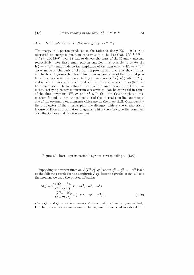
decay mode on the basis of the Born approximation diagrams shown in fig.4.7. In these diagrams the photon line is hooked onto one of the external pionlines. The Kππ vertex is represented by a function F (P 2, q2+, q

2−), where P , q+

and q− are the momenta associated with the K- and π-meson lines (here wehave made use of the fact that all Lorentz invariants formed from three mo-menta satisfying energy momentum conservation, can be expressed in termsof the three invariants P 2, q2+ and q2− ). In the limit that the photon mo-mentum k tends to zero the momentum of the internal pion line approachesone of the external pion momenta which are on the mass shell. Consequentlythe propagator of the internal pion line diverges. This is the characteristicfeature of Born approximation diagrams, which therefore give the dominantcontribution for small photon energies.

Figure 4.7: Born approximation diagrams corresponding to (4.92).

Expanding the vertex function F (P 2, q2+, q2−) about q

2+ = q2− = −m2 leads

to the following result for the amplitudeMBµ from the graphs of fig. 4.7 (for

the moment we keep the photon off shell):

MBµ = e

(2Q+ + k)µk2 + 2k ·Q+

F (−M2,−m2,−m2)

− (2Q− + k)µk2 + 2k ·Q−

F (−M2,−m2,−m2), (4.89)

where Q+ and Q− are the momenta of the outgoing π+ and π−, respectively.For the γππ-vertex we made use of the Feynman rules listed in table 4.1. It


is important to observe that the amplitude (4.89) is conserved, because

kµMBµ = e

(2k ·Q+ + k2)

k2 + 2k ·Q+− (2k ·Q− + k2)

k2 + 2k ·Q−

F (−M2,−m2,−m2) = 0 .

(4.90)

One may deduce that the remaining contributions to the full amplitude mustbe linear in the photon momentum. To see this one notes that a conservedamplitude depending on the three independent momenta in this process, Q+,Q− and k, can be parametrized as a sum of two terms, namely

Mµ = A(k ·Q−Q+µ − k ·Q+Q−µ) +BεµνρσQ+νQ−ρkσ . (4.91)

Since (4.89) is conserved and represents all contributions to the full amplitudethat are singular in the k → 0 limit the remaining terms in the amplitude musttake the form of (4.91) with coefficients A and B that are finite in this limit.Because (4.91) is already linear in k the full amplitude must satisfy

Mµ = e (2Q+ + k)µk2 + 2k ·Q+

− (2Q− + k)µk2 + 2k ·Q−

F (−M2,−m2,−m2) +O(k) .

(4.92)

Setting also the photon on the mass shell we may now conclude that theinvariant amplitudes for the radiative and nonradiative decay are related by

εµMµ(K0S → π+π−γ) = −e

( ε ·Q−k ·Q−

− ε ·Q+

k ·Q+

)M(K0

S → π+π−) +O(k) ,

(4.93)

whereM(K0S → π+π−) = F (−M2,−m2,−m2) does not depend on the exter-

nal momenta. Squaring (4.93) and summing over photon polarizations leadsto

∑

pol

|εµMµ(K0S → π+π−γ)|2

= e2( Q−µk ·Q−

− Q+µ

k ·Q+

)2|M(K0

S → π+π−)|2 +O(k0)

= e2 −2Q+ ·Q−(k ·Q+)(k ·Q−)

− m2

(k ·Q+)2− m2

(k ·Q−)2|Mµ(K

0S → π+π−)|2

+O(k0) , (4.94)

where we have used (4.41). For the moment we ignore the fact that (4.94)diverges for small photon energies. This so-called infrared divergence is caused


by the fact that the photon is massless. We return to this aspect at the endof this section.The rate for the nonradiative decay follows from (3.82). The result is

Γ (K0S → π+π−) =

β016πM

|M(K0S → π+π−)|2 , (4.95)

where β0 is the pion velocity in the rest frame of the K meson,

β0 =

√1− 4m2

M2, (4.96)

which equals the maximal possible pion velocity for the radiative decay.For the radiative decay we use the expression (3.105) for the phase space

integral, where m1 = 0 and m2 = m3 = m. In the parametrization (3.101)ω = ω1 denotes the photon energy and ω2 and ω3 the pion energies in the restframe of K0

S . Using momentum conservation it is easy to show that

2k ·Q+ = −M(ω + 2x) , 2k ·Q− = −M(ω − 2x) ,

2Q+ ·Q− = −M2 + 2Mω + 2m2 . (4.97)

Since the amplitude does not depend on the orientation of the decay plane,we may integrate (3.105) over the corresponding three angles. This leads to afactor 8π2. According to the definition (3.79) we must divide (3.105) by 2Min order to obtain the decay rate. Substituting the combined results of (4.94)and (4.97) then gives (dropping the unknown O(k0) terms)

Γ (K0S → π+π−γ) =

e2

16π3M3|M(K0

S → π+π−γ)|2

×∫ ωm

0

dω

∫ x+

x−

dxM2 − 2Mω − 2m2

(ω + 2x)(ω − 2x)− m2

(ω + 2x)2− m2

(ω − 2x)2

,(4.98)

where according to (3.104) and (3.102)

x± = ± 12ω

√ωm − ω

ωm − ω + 2m2/M,

ωm = 12Mβ2

0 . (4.99)

It is convenient to introduce a parameter

β =

√M2 − 2Mω − 4m2

M2 − 2Mω, (4.100)

which corresponds to the pion velocity measured in the rest frame of the twopions (see problem 4.8) (in the limit that ω → 0, this frame coincides with


the rest frame of the K meson and β → β0). The parameters x± now take theform

x± = ± 12βω . (4.101)

The necessary x-integrals for (4.98) are simple and are given by

∫ x+

x−

dx1

(ω + 2x)(ω − 2x)=

1

ωlnω + 2x

ω − 2x

∣∣∣x+

x−

=1

4ωln

1 + β

1− β ,∫ x+

x−

dx1

(ω ± 2x)2= ∓ 1

2

1

ω ± 2x

∣∣∣x+

x−

=β

ω(1− β2). (4.102)

Hence

Γ (K0S → π+π−γ)

Γ (K0S → π+π−)

=α

π

∫ 12Mβ2

0

0

dω

ω

1 + β2

βln

1 + β

1− β − 2 ββ0

(1− 2ω

M

).

(4.103)

where α is the fine-structure constant.As anticipated previously, (4.103) diverges if the photon energy ω tends

to zero. Nevertheless, this result can be compared to experiment, because inan experimental situation there is always a minimal photon energy ω0 belowwhich it is impossible to detect the photons emitted. Therefore the relevantradiative decay rate is

Γ (K0S → π+π−γ;ω > ω0)

Γ (K0S → π+π−)

=α

π

∫ 12Mβ2

0

0

dω

ω

1 + β2

βln

1 + β

1− β − 2 ββ0

(1− 2ω

M

). (4.104)

Figure 4.8 shows the measured photon spectrum in the range 25 MeV< ω <175 MeV. For ω > ω0 = 50 MeV the data show an ω−1 behaviour consistentwith the ω−1 behaviour of the integrand in (4.104). Note that the shape of thehistogram for ω < ω0 reflects the photon trigger efficiency. For ω0 = 50 MeVthe integral in (4.104) gives the numerical value of 2.54×10−3, in excellentagreement with the result of the same experiment which quotes

Γ (K0S → π+π−γ;ω > 50MeV)

Γ (K0S → π+π−)

= (2.68± 0.15)× 10−3 . (4.105)

But how do we interpret the part of the integral (4.103) where ω < ω0? Sincethe photons are not observed in this energy range the corresponding eventswould be counted as genuine K0

S → π+π− decays. Consequently the relevant


definition of the decay rate for K0S → π+π− must be changed in order to

account for unobservable soft photons. Hence to order α we have

Γ (K0S → π+π−) =

β

16πM|F (−M2,−m2,−m2)|2

×1 +

α

π

(1 + β20

β0ln

1 + β01− β0

− 2)∫ ω0

0

dω

ω

,(4.106)

where we have reintroduced the vertex function F and approximated theintegral (4.103) for small values of ω. Of course, the minimal observable photonenergy ω0 depends on the experiment under consideration. The extra termsin (4.109) are called radiative corrections.

Figure 4.8: Distribution of events with photon energy ω in the K0 rest frame.The events above ω0 = 50 MeV reflect the ω−1 behaviour as given in (4.104),whereas the shape of the histogram below ω0 reflects the efficiency of thephoton trigger. [H. Taureg, G. Zech, F. Dydak, F. L. Navarria, P. Steffen, J.Steinberger, H. Wahl, E. G. H. Williams, C. Geweniger and K. Kleinknecht,Phys. Lett. 65B (1976) 92.]

The divergent part of the integral (4.103) thus appears in the nonradiativedecay rate as a correction of order α. However, it is important to observe thatthere are other corrections to this process in the same order of α. These cor-rections originate from virtual photons, and also lead to infrared divergences.


The calculation of the nonradiative decay rate now involves additional graphsas is schematically shown in fig. 4.9. At this point it is convenient to introducea small photon mass κ to give a more precise definition of the infrared diver-gences. The integral in (4.106) from the bremsstrahlung graphs then gives adivergent term proportional to lnω0/κ. The corrections from the virtual pho-ton diagrams lead to terms proportional to lnκ/M . Hence both contributionsdiverge logarithmically when κ → 0, but, surprisingly enough, these two di-vergences cancel in the decay rate, so that the answer contains only a termlnω0/M , where ω0 is a finite number that may change from experiment to ex-periment. The procedure by which these infrared divergences cancel was firstdescribed by Bloch and Nordsieck. Later it was shown that this cancellationholds to all orders in α (higher-order terms usually generate an exponentialseries). In section 8.6 we will explicitly establish the cancellation of infrareddivergences to lowest nontrivial order in a different process.

Figure 4.9: Order α diagrams contributing to the decay rate for K0S → π+π−.

Thus we see that the emission of photons from charged particles gives rise toeither radiative processes, in which the photon is properly identified, or radia-tive corrections to nonradiative processes in which the photon identification isnot possible. We should add that the virtual photon corrections may lead toinfrared divergences when the photon momentum is small and to ultravioletdivergences when the momentum is large (we will learn how to interpret thelatter divergences in due course). After both divergences have been eliminatedorder by order in perturbation theory the remaining finite terms should agreewith experimental results. The evaluation of these finite corrections is rathercomplicated. For that reason we have relegated a technical discussion of someof the necessary integrals to appendix D.

Problems 149

Problems

4.1. Consider the decay of a vector particle V with momentum P into two scalarsS1, and S2 with momenta p1; p2 (p21 = −m2

1 , p22 = −m2

2, P2 = −M2). Show that the

decay amplitude for the process generally takes the form

Mµ(p1, p2) = i(p1 + p2)µf(P2, p21, p

22) + i(p1 − p2)µg(P

2, p21, p22) (1)

by exploiting Lorentz invariance. Argue that f does not contribute to the decayrate, so that the decay is precisely described by an effective Lagrangian

L = gVµ(φ1

↔∂ µφ2) (2)

Consider the decay V→ S1S2 with S1 emitted in the x− z plane at an angle θ withrespect to the z-axis. Show that the differential decay rates for polarization statesof the V with spin Sz = ±1 and 0 along the z-direction are proportional to sin2 θand cos2 θ respectively. Integrate these expressions over θ to find the decay rate,

Γ =g2

48π

λ3/2(M2,m21,m

22)

M5(3)

for each spin state. Note that the total decay rate for an unpolarized V is also givenby (3).As an example consider the decay of rho mesons into pions. Just as the pion fieldscan be written as real isospin vectors πa (cf. 2.54) the rho fields can be treatedin the same way, i.e. ρ0 = ρ3,

√2ρ± = ρ1 ∓ iρ2. Argue that the isospin invariant

generalization of (2) is

L = gεijkV iµ(φ

j↔∂ µφ

k) . (4)

Write this Lagrangian in terms of the ρ±, ρ0, π±, and π0 fields. Calculate the decayrates for ρ+ → π+π0, ρ0 → π+π−, ρ0 → π0π0 and show that they are in the ratio1:1:0.

4.2. Consider a massive vector boson coupled to a conserved current so that theamplitude equals M = εµ(k)Mµ(k) where kµMµ = 0. Show that, although thelongitudinal polarization vector is singular in the limit m → 0 (cf. 4.11b), the am-plitude vanishes for longitudinal vector bosons in this limit. This property makes ithard to distinguish between an almost massless and a massless photon. [For boundson the photon mass see A. Goldhaber and M. M. Nieto, Rev. Mod. Phys. 43 (1971)227.] The smooth decoupling of the longitudinal polarization in the massless limitturns out to be a special property of neutral vector bosons. For instance it does nothold for gravitons (the spin-2 quanta of gravitation) where there is a discontinuityat m = 0 [H. van Dam and M. Veltman, Nucl. Phys. B22 (1970) 397; see also M.Veltman, in: Methods in Field Theory, Les Houches 1975, eds. R. Balian and J.Zinn-Justin (North-Holland/World Scientific, 1976) p. 266.]

4.3. Using the Lagrangian of problem 4.1, calculate the amplitude for the reactionπ+ + π− → π+ + π− in tree approximation.


When s = M2 one should take into account that the ρ0 is not a stable particle.Therefore the propagator factor s − M2 becomes s − M2 + iMΓ where Γ is thetotal decay rate in the rest frame. Now evaluate the differential cross section in thecentre-of-mass frame, which in the limit M → 0 and Γ → 0 can be compared to(4.51). Integrate this result to find the total cross section as a function of s, andcompare your answer with (3.92). Observe the factor of 3 and verify that this agreeswith the discussion in the text after (3.92).

4.4. To describe the interactions of photons with charged massive vector particles,consider (4.1) for two real fields W 1

µ and W 2µ , change to a complex basis described

by√2Wµ =W 1

µ − iW 2µ ,

√2Wµ =W 1

µ +iW 2µ and apply the minimal electromagnetic

substitution as in section 4.3. Note that Wµ ≡ (1− 2δµ4)W∗µ transforms as a vector

under Lorentz transformations (cf A.24). Show that the resulting Lagrangian is

L1 = − 12(∂µWν − ∂νWµ)(∂µWν − ∂νWµ)−M2WµWµ

−ieAµ[Wν(∂µWν − ∂νWµ)− (∂µWν − ∂νWµ)Wν ]

−e2(AµAνWνWµ −AµWµAνWν) . (1)

Verify the invariance of (1) under electromagnetic gauge transformations (cf. 4.43):

Aµ(x) → Aµ(x) + ∂µξ(x) , Wµ(x) → eieξ(x)Wµ(x) . (2)

It is possible to add to (1) a term that is separately gauge invariant, namely

L = −ieκ(∂µAν − ∂νAµ)WµWν , (3)

which in the particle rest frame describes an additional coupling with the magneticfield. Therefore (3) is called the anomalous magnetic moment term.Using k, p and r as incoming particle momenta for the fields Aµ, Wρ and Wσ,respectively, show that the three-point vertex corresponding to (1) and (3) is

Vµρσ(k, p, r) = e[(κk − p)σηµρ + (p− r)µηρσ + (r − κk)ρηµσ] , (4)

where we have suppressed the usual factor i(2π)4δ4(k + p+ r).Construct the invariant amplitude for a virtual photon interacting with an incomingand outgoing W+,

Mµ(p2, p1) = eεσ(p2)[(p1+p2)µηρσ+(1+κ)((p2−p1)σηρµ−(p2−p1)ρησµ]ερ(p1) ,

(5)

where ερ(p1) and p1 (εσ(p2) and p2) are the polarization vector and momentumof the incoming (outgoing) W+. The two terms in (5) characterize the coupling ofthe photon to the charge and the magnetic moment of the vector particle. Observethat the magnetic moment coupling is proportional to 1+ κ. Prove that the photoncouples to a conserved current, i.e. (p2 − p1)µMµ(p2, p1) = 0. Compare (5) to thecorresponding expression for the coupling of a virtual photon to an incoming and

Problems 151

outgoing π+. Show that the square of (5), averaged over incoming W polarizationsand summed over outgoing W polarizations, equals

Wµν ≡ 13

∑

spins

Mµ(p2, p1)Mν(p2, p1)

= 13e2

2(1 + κ)2(

1 +Q2

4M2

)

(Q2ηµν −QµQν)

+(

3 + (1 + κ2)Q2

2M2+ κ2 Q4

4M4

)

PµPν

, (6)

where Q = p2 − p1 , P = p2 + p1 (so that P · Q = 0). Note that (6) satisfiesQµWµν =WµνQν = 0.Repeat this analysis for the pion vertex using Q = q1 − q2, R = q1 + q2 (so thatQ ·R = 0) to find the corresponding tensor

Lµν = e2RµRν , (7)

which satisfies QµLµν = LµνQν = 0.Write the square of the amplitude for the electromagnetic scattering process

π+(q1) +W+(p1) → π+(q2) +W+(p2)

in terms of (6) and (7). Using s = −(p1+ q1)2, t = −(p1−p2)2 and u = −(p1− q2)2,

show that the invariant differential cross section is

dσ

dt=

πα2

λ(s,M2,m2)

1

3t2

×(

3− (1 + κ2)t

2M2+ κ2 t2

4M4

)

(u− s)2

−2(1 + κ)2t(t− 4m2)(

1− t

4M2

)

. (8)

Express this result in terms of the laboratory scattering angle using (4.54) andcompare the answer with (4.55).Now consider the invariant amplitude for Compton scattering (i.e. γ +W+ → γ +W+). Include the contribution from the four-point vertex corresponding to (1)

Vµνρσ(k, q, p, r) = −e2[2ηµνηρσ − ηµρηνσ − ηµσηνρ] , (9)

where k, q, p and r are the incoming momenta for the fields Aµ, Aν , Wρ and Wσ.Keep the photons off-shell and show that the Compton amplitude is transverse (cf.section 4.4).

4.5. To illustrate that the gauge-fixing term (4.35) only introduces an extra degreeof freedom into the theory which does not interfere with the interactions (cf., thediscussion leading to 4.35), consider the Maxwell theory coupled to a conservedsource, i.e.

L = − 14FµνFµν + JµAµ (1)


with ∂µJµ = 0. After the addition of (4.35) the field equation for Aµ is

∂µFµν + Jµ + λ2∂ν(∂ ·A) = 0 . (2)

Contracting this with another derivative leads to the free field equation for ∂ ·A i.e.,

(∂ ·A) = 0. (3)

To be more specific one can take the theory given by (4.42) for charged pions coupledto photons. In this model the current corresponds to

Jµ = −ieφ∗↔∂ µφ− 2e2Aµ|φ|2 . (4)

Show that this current is conserved as a result of the pion equations of motion, sothat (3) will be satisfied in the presence of the gauge-fixing term (4.35).

4.6. From (4.64) derive the following formula for pion Compton scattering, whereθCM is the photon scattering angle in the centre-of-mass system

dσ

dΩCM=α2

s

(s2 +m4)(1 + cos2 θCM) + 2(s2 −m4) cos θCM

[s+m2 + (s−m2) cos θCM]2.

Integrate this equation to find the total cross section,

σ =4πα2

s

(s+m2

s−m2

)[

1− 2m2s

(s+m2)(s−m2)ln

s

m2

]

.

4.7. Consider the interaction Lagrangian involving the photon field Aµ, the neutralpion field φ and a massive charged spinless field Φ associated with a nucleus N ofcharge Ze:

L = iαCεµνρσFµνFρσφ− iZeAµ[Φ∗∂µΦ− Φ(∂µΦ

∗)] . (1)

Write down the order Ze3 amplitude for the photoproduction process γ(k1) +N(P1) → π0(k2) + N(P2), often called the Primakoff process. Use invariantss = −(k1 +P1)

2, t = −(k1 − k2)2 and u = −(k1 −P2)

2 and calculate the differentialcross section in the centre-of-mass frame,

dσ

dΩCM=αZ2Γ (π0 → γγ)

2sm3πt2

√

λ(s,m2π,M2)

λ(s, 0,M2)[(t− 4M2)(m2

π − t)2 − t(u− s)2] . (2)

Now take the limit that M → ∞ (static nucleus) and show that

dσ

dΩlab=

8αZ2Γ (π0 → γγ)

m3π

β3(ω2

t

)2

sin2 θ . (3)

where β =√

1−m2π/ω2 , ω is the photon energy, and θ the laboratory angle of the

outgoing π0. For a measurement of Γ (π0 → γγ) using this process see A. Browman,

References 153

J. DeWire, B. Gittelman, K. M. Hanson, D. Larson, E. Loh and R. Lewis, Phys.Rev. Lett. 33 (1974) 1400.

4.8. Consider the kinematics of the reaction K0S(P ) → π+(Q+) + π−(Q−) + γ(k).

Define the invariant mass√s of the π+π− system by s = −(Q+ + Q−)

2 and showthat s = M2 − 2Mω. Since s is a Lorentz-invariant quantity one can go to thecentre-of-mass frame of the π+π− system and calculate the pion velocities in termsof s. Use this method to show that the velocity is equal to β given in (4.100).

4.9. The K0L-meson has a small CP -violating decay rate into π+π− ,so the the

corresponding bremsstrahlung amplitude for the decay K0L → π+π− is suppressed.

However, there is also a direct (magnetic dipole) transition which contributes tothe decay rate. The corresponding interaction Lagrangian expressed in terms of thefields Aµ, φ, φ

∗ and φK for γ, π+, π− and K0L, respectively, is

Lint =eg

M3εµνρσFµν∂ρφ

∗∂σφφK ,

where the K mass is denoted by M and g is a dimensionless constant. Show thatthe photon spectrum resulting from this interaction is given by

dΓ (K0L → π+π−γ)

dω=

αg2

24π2M3ω3β3

(

1− 2ω

M

)

,

where β is given by (4.100) and ω is the photon energy in the K0L rest frame. Note

that this result remains finite when ω → 0. For a measurement of this spectrum seeA. S. Carroll, I.-H. Chiang, T. F. Kycia, K. K. Li, L. Littenberg, M. Marx, P. O.Mazur, J. P. de Brion and W. C. Carithers, Phys. Rev. Lett. 44 (1980) 529.

References

The field equation for massive vector mesons was introduced by A. Proca, J.Phys. Radium 9 (1938) 61. The original references on Rutherford, Compton and

Thomson scattering E. Rutherford, Philos. Mag. 21 (1911) 669.A. H. Compton, Phys. Rev. 21 (1923) 207, 483.J. J. Thomson, Conduction of Electricity through Gases, 3rd Ed., Vol. 11 (Cambridge

University Press, 1933) p. 256. For the latest data on Compton scattering on pions

M. Zielinski et al., Phys. Rev. D29 (1984) 2633. For a review of Compton scattering

on nucleons H. Rollnick and P. Stichel. Compton Scattering,Elementary Particle Physics Series, Vol. 7 Springer, New York, 1976). References

for our discussion of the decay π0 → γγ J. Steinberger, Phys. Rev. 76 (1949)1180.

C. N. Yang, Phys. Rev. 77 (1949) 242.E. Karlson, Ark. Fys. 13 (1958) 1.


N. P. Samios, R. Plano, A. Prodell, M. Schwartz and J. Steinberger, Phys. Rev. 126(1962) 1844.

T. Mijazaki and E. Takasugi, Phys. Rev. D8 (1973) 2051. For the Goldherger-

Treiman relation M. L. Goldberger and S. B. Treiman, Phys. Rev. 110 (1958)1178; 111 (1958) 354.

S. L. Adler and R. F. Dashen, Current Algebras (Benjamin, New York, 1968).Theoretical papers on the treatment of infrared divergences F. Bloch and A.

Nordsieck, Phys. Rev. 52 (1937) 54, 59.D. R. Yennie, S. C. Frautschi and H. Suura, Ann. Phys. 13 (1961) 379.G. Grammer and D. R. Yennie, Phys. Rev. D8 (1973) 4332.

Particles with spin one - Nikheft45/ftip/Ch04.pdf · number of independent plane-wave solutions of...

Documents

Transcript of Particles with spin one - Nikheft45/ftip/Ch04.pdf · number of independent plane-wave solutions of...