Particle-Imaging Techniques for Experimental Fluid...

Annu. Rev. Fluid Mech. 1991.23 : 261 304Copyright © 1991 by Annual Reviews Inc. All rights reserved

PARTICLE-IMAGINGTECHNIQUES FOREXPERIMENTAL FLUIDMECHANICS

Ronald J. Adrian

Department of Theoretical and Applied Mechanics, University of Illinois,Urbana, Illinois 61801

KEY WORDS: experimental fluids, turbulence, measurements, laser velocimetry

INTRODUCTION

An important achievement of modern experimental fluid mechanics is theinvention and development of techniques for the measurement of whole,instantaneous fields of scalars and vectors. These techniques include tomo-graphic interferometry (Hesselink 1988) and planar laser-induced fluo-rescence for scalars (Hassa et al 1987), and nuclear-magnetic-resonanceimaging (Lee et al 1987), planar laser-induced fluorescence, laser-specklevelocimetry, particle-tracking velocimetry, molecular-tracking velocimetry(Miles et al 1989), and particle-image velocimetry for velocity fields.Reviews of these methods can be found in articles by Lauterborn & Vogel(1984), Adrian (1986a), Hesselink (1988), and Dudderar et al (1988), in books written by Merzkirch (1987) and edited by Chiang & Reid (1988)and Gad-el-Hak (1989).

Pulsed-Light Velocimetry

The subject of the present article, particle-imaging techniques, is a memberof a broader class of velocity-measuring techniques that measure themotion of small, marked regions of a fluid by observing the locations ofthe images of the markers at two or more times. These methods return to

2610066-4189/91/0115-0261 $02.00

www.annualreviews.org/aronlineAnnual Reviews

Ann

u. R

ev. F

luid

Mec

h. 1

991.

23:2

61-3

04. D

ownl

oade

d fr

om a

rjou

rnal

s.an

nual

revi

ews.

org

by I

owa

Stat

e U

nive

rsity

on

03/1

7/07

. For

per

sona

l use

onl

y.

http://www.annualreviews.org/aronline

262 ADRIAN

the fundamental definition of velocity and estimate the local velocity ufrom

Ax(x, (i)u(x,t) =" At

where Ax is the displacement of a marker, located at x at time t, over ashort time interval At separating observations of the marker images. Theparticles are usually solids in gases or liquids but can also be gaseousbubbles in liquids or liquid droplets in gases or immiscible liquids. Othertypes of markers include (a) patches of molecules that are activated laser beams, causing them either to fluoresce (Gharib et al 1985), or change their optical density by photochromic chemical reactions (Popovich& Hummel 1967, Ricka 1987), and (b) speckle patterns caused by illumi-nating groups of particles with coherent light. Regardless of the markertype, locations at various instants are recorded optically by pulses of lightthat freeze the marker images on an optical recording medium such as aphotographic film, a video array detector, or a holographic film. Sincethese methods share many similarities, it is useful to group them under thesingle topic of pulsed-light veloeimetry, or PLV.

The various PLV techniques are organized in Figure 1.

Particle-Image VelocimetryA technique that uses particles and their images falls into the categorycommonly known as particle-image velocimetry, or PIV, which is theprincipal subject of this article. Before comparing the characteristics ofPIV with the other methods displayed in Figure 1, it is helpful to examine

Pul~ed Light VeloclmetryPLV

Figure 1 Particle-image velocimetry and other forms of pulsed-light velocimctry.


Ann

u. R

ev. F

luid

Mec

h. 1

991.

23:2

61-3

04. D

ownl

oade

d fr

om a

rjou

rnal

s.an

nual

revi

ews.

org

by I

owa

Stat

e U

nive

rsity

on

03/1

7/07

. For

per

sona

l use

onl

y.


PARTICLE-IMAGING TECHNIQUES 263

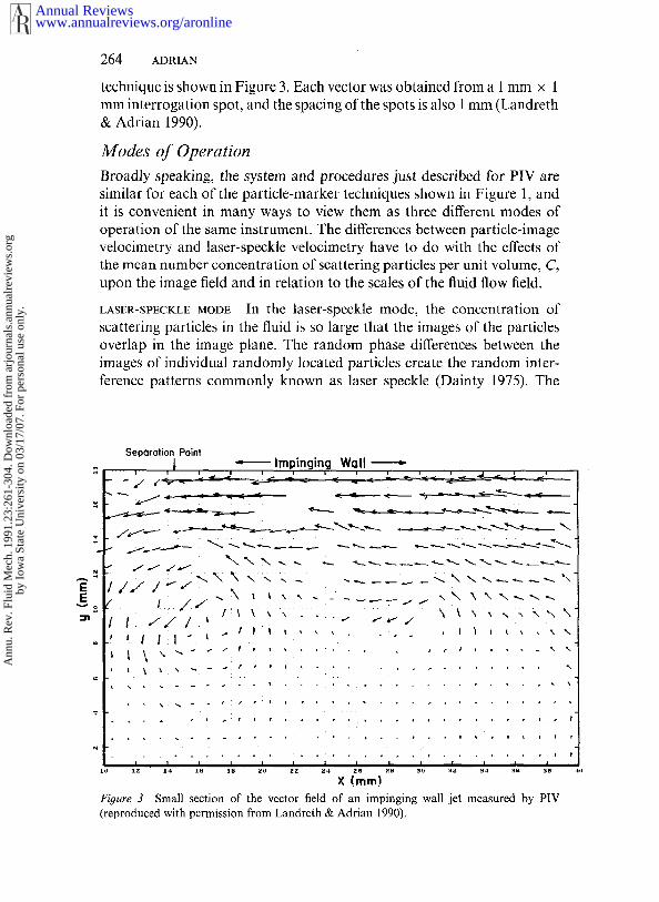
a typical PIV system in somewhat greater detail. To this end, a planarparticle-image velocimeter optical system is shown in Figure 2. Particlesin the fluid are illuminated by a sheet of light that is pulsed. The particlesscatter light into a photographic lens located at 90° to the sheet, so thatits in-focus object plane coincides with the illuminated slice of fluid. Imagesare formed on a photographic film or on a video array detector, and theimages are subsequently transferred to a computer for automatic analysis.The analysis of the recorded image field is one of the most important stepsin the entire process, as it couples with the image-acquisition process todetermine the accuracy, reliability, and spatial resolution of the measure-ments; it is also the most time-consuming part of the process. Imageanalysis, or "interrogation," is discussed in detail later. If the recordedimage field contains a small amount of information, as for a typical videocamera that consists of an array of approximately 500 × 500 pixels, theentire image field (e.g. 2.5 × 105 pixels) can be digitized and passed to thecomputer in one file. If the image field is very rich in information, as fora 100 mm× 125 mm piece of 300 lines ram-’ resolution photographicfilm containing over 1.1 × 109 pixels, the local velocity in a small regionof the image field is found by digitizing an interrogation spot and analyzingthe images within the spots, one spot at a time. The vector field is obtainedby repeating this process on a grid of such interrogation spots.

An example of a small portion of a vector field measured by the latter

FOCAL LENGTH f

VIDEO ARRAY

-..:....- ....

doT d,- f I

Figure 2 Optical system of a planar particle-image velocimeter, (Top) Video recording;(bottom) photographic recording.


Ann

u. R

ev. F

luid

Mec

h. 1

991.

23:2

61-3

04. D

ownl

oade

d fr

om a

rjou

rnal

s.an

nual

revi

ews.

org

by I

owa

Stat

e U

nive

rsity

on

03/1

7/07

. For

per

sona

l use

onl

y.


264 ADRIAN

technique is shown in Figure 3. Each vector was obtained from a 1 mmx 1mm interrogation spot, and the spacing of the spots is also 1 mm (Landreth& Adrian 1990).

Modes o j Operation

Broadly speaking, the system and procedures just described for PIV aresimilar for each of the particle-marker techniques shown in Figure 1, andit is convenient in many ways to view them as three different modes ofoperation of the same instrument. The differences between particle-imagevelocimetry and laser-speckle velocimetry have to do with the effects ofthe mean number concentration of scattering particles per unit volume, C,upon the image field and in relation to the scales of the fluid flow field.

LASER-SPECKLE MODE In the laser-speckle mode, the concentration ofscattering particles in the fluid is so large that the images of the particlesoverlap in the image plane. The random phase differences between theimages of individual randomly located particles create the random inter-ference patterns commonly known as laser speckle (Dainty 1975). The

X (ram)

Figure 3 Small section of the vector field of an impinging wall jet measured by PIV(reproduced with permission from Landreth & Adrian 1990).


Ann

u. R

ev. F

luid

Mec

h. 1

991.

23:2

61-3

04. D

ownl

oade

d fr

om a

rjou

rnal

s.an

nual

revi

ews.

org

by I

owa

Stat

e U

nive

rsity

on

03/1

7/07

. For

per

sona

l use

onl

y.



local speckle pattern is the superposition of images from a local group ofscattering particles, and as such it translates with the group of particles.Hence, velocity can be measured by measuring speckle displacement, andoperation in this mode is called laser speckle velocimetry, or LSV.

PARTICLE-TRACKING MODE In the particle-image mode the concentrationof scatterers is low enough to render overlapping images improbable, andindividual particle images dominate. Within this regime of concentrations,two limits exist. In the low-image-density limit the concentration of scat-terers is so small that images are sparse in the image plane. Multipleexposures or streak exposures of individual particles leave tracks that areshort compared with the mean spacing between particles, so that individualimages are easily identified. Since the number of images per unit area issmall, it is feasible to measure displacements by tracking individual images.Hence, the low-image-density mode of PIV is often referred to as particle-tracking velocimetry, or PTV.

HIGH-IMAGE-DENSITY PIV MODE The high-image-density mode of PIVoccurs when concentrations lie between those of LSV and PTV. Theconcentrations are high enough to guarantee that every interrogation spotin the image field contains many images, but not so high that the imagesoverlap to produce speckle. In this mode, the abundance of images makestracking individual particles time consuming, and one measures insteadthe displacements of small groups of images.

Historical Development

Although it is useful to view high-image-density PIV and PTV as limitingextremes of the general class of particle-imaging techniques in order tounify that part of the theory and practice that is common to each, thisunification does not reflect the historical development of these techniques.Many of the approaches used in PTV are natural extensions of classicalflow-visualization techniques, whereas many elements of low-image-den-sity PIV and especially high-image-density P|V grew out of laser-specklevelocimetry.

Particle-tracking velocimetry has its roots in flow-visualization tech-niques such as particle-streak photography and stroboscopic photography,of which several beautiful examples can be found in Van Dyke (1982).Because of the simplicity of the particle-tracking concept, quantitative (orat least semiquantitative) results have been available from this techniquefor decades, provided one was willing to perform manual analysis (cf Fage& Townend 1932). The thrusts of modern developments in PTV have beento make the technique more quantitative and to computerize the analysisof images.


Ann

u. R

ev. F

luid

Mec

h. 1

991.

23:2

61-3

04. D

ownl

oade

d fr

om a

rjou

rnal

s.an

nual

revi

ews.

org

by I

owa

Stat

e U

nive

rsity

on

03/1

7/07

. For

per

sona

l use

onl

y.


266 ADRIAN

Laser-speckle velocimetry has its roots in solid mechanics, where coher-ent light scattered from solid surfaces naturally forms speckle patterns(Erf 1980, Archbold & Ennos 1972). Unlike PTV, simple manual analysisof a double-exposed specklegram is not feasible, because the human eyecannot untangle the superposed speckle fields. Analysis of such fieldsbecame possible with the development of the Young’s fringe method ofinterrogation (Burch & Tokarski 1968, Stetson 1975) in which an interro-gation spot on a double-exposed specklegram is illuminated by a laser beam.The speckle field from each exposure diffracts a light wave from thecoherent interrogation beam, which interferes with the other wave to forma Young’s fringe pattern (Figure 4). The orientation of the fringes perpendicular to the direction of the displacement, and the spacing isinversely proportional to the magnitude of the displacement. This tech-nique addressed the issue of comparing the speckle field from the first

INTERROGATION

~ Specklegram or PIV photo~ I I on computer controlled VIDEO ARRAY

"~--.~_~.~..~ ~y table

~ Interrogation spot LX

beom ~i~- ~ ~ ............. ~ Young’s

AX=MuAt 0

Figure 4 Interrogation of a photograph. (Top) Direct-image digitization; (bottom) Young’sfringe method in which a lens performs on an optical two-dimensional Fourier transform ofthe image field in the interrogation spot.


Ann

u. R

ev. F

luid

Mec

h. 1

991.

23:2

61-3

04. D

ownl

oade

d fr

om a

rjou

rnal

s.an

nual

revi

ews.

org

by I

owa

Stat

e U

nive

rsity

on

03/1

7/07

. For

per

sona

l use

onl

y.



exposure with the field from the second exposure and statistically pairingthem speckle by speckle.

Early experiments by Dudderar & Simpkins (1977), Grousson & Mallick(1977), and Barker & Fourney (1977) showed that the laser-speckle tech-nique could be applied to measure fluid motion in simple, steady laminarflows using the Young’s fringe method of interrogation. Simpkins & Dud-derar (1978) and Meynart (1980, 1983a,b,c, 1985) pioneered much of development of LSV and its application to more complex flows, includinga turbulent jet and thermal convection.

High-image-density particle-image velocimetry was established as a dis-tinct mode of pulsed-light velocimetry by Pickering & Halliwell (1984) andAdrian (1984), who argued that the concentrations of scattering particlesthat are practical in experimental fluid mechanics are often not denseenough to create speckle patterns. Thus, unless one makes extreme effortsto seed the flow with high concentrations of carefully chosen particles,high-image-density PIV is more likely than LSV. Many experiments thathad been labeled LSV were indeed PIV, as Meynart (1983a) seems to haverecognized. Further studies of the scattering properties of particles inrelation to photographic imaging (Adrian & Yao 1985) indicated thatindividual particles in the 1-10 #m range would produce more detectableimages at lower mass loadings than the large numbers of fine particles thatwould be needed to produce speckle. This result is much like the findingin laser-Doppler velocimetry that it is better to use incoherent detectionthan coherent detection in most cases (Drain 1972).

Although high-image-density PIV resembles LSV in many regards, thisarticle focuses on the particle-image mode, with the proviso that many ofthe concepts and developments will be applicable to LS¥ as well. Topicsthat are common to particle imaging in general are discussed first, followedby separate sections for the high- and low-image-density cases.

PARTICLES AND THEIR IMAGES

Single-Particle Ima.qin9

Given an ideal, aberration-free lens of focal length f, the image of a smallparticle at x in the fluid is mapped onto the point -q in the image planeof the lens, where

~ = ao-~ [x~ +y~]. (2)

Here do and d~ are the object and image distances, respectively, i and ~ areunit vectors perpendicular to the optic axis of the lens, and z is the distance


Ann

u. R

ev. F

luid

Mec

h. 1

991.

23:2

61-3

04. D

ownl

oade

d fr

om a

rjou

rnal

s.an

nual

revi

ews.

org

by I

owa

Stat

e U

nive

rsity

on

03/1

7/07

. For

per

sona

l use

onl

y.


268 ADRIAN

away from the object plane. The magnification depends upon z accordingto

M(z) - do - (3)

and this dependence embodies the usual rules of perspective. In particular,it is noted that erecting the image takes -r/into t/, so that a small dis-placement of a particle in the fluid results in an erected-image displacementgiven by

= M(0) (Ax~ + Aye) + M(0) (xr2ffoY~) Az. (4)AX

These equations refer to coordinates centered on the camera axis and ideallenses. Generalized equations for arbitrary coordinates and lenses withaberrations are presented by Murai et al (1980).

The intensity of the image in the nominal image plane at di, per unit ofilluminated beam intensity Io(t), is denoted by ~o(X + t/(x); x). The diam-eter of the image is determined by the diameter of the particle dp, themagnification, and the point response function of the lens. If the lens isdiffraction limited, the point response function is an Airy function ofdiameter

ds = 2.44(1 +M)f#2, (5)

wheref# is the f-number of the lens, and 2 is the wavelength of light. Theimage of a finite-diameter particle is the convolution of the Airy functionwith the geometric image of the particle (Goodman 1968). Approximatingboth functions by Gaussians leads to the following approximate formulafor the image diameter (Adrian & Yao 1985):

de --_ (MZd~ + d2~ )1/2. (6)

For typical values of the parameters (say M = l, f# = 8, and 2 = 0.6993/~m), ds = 25 #m, so de is approximately independent of the particle sizefor particle diameters less than about 10 #m. Conversely, for particlediameters greater than 50/~m, the image diameter is essentially Mdp.

The foregoing equations pertain when the particle is within the depthof field of the lens, given by

6z = 4(l+M 1)~c#22.’ (7)

Outside of this range the image is blurred by an amount exceeding 20%

~ This formula, due to P. W. Offutt, generalizes the conventional result to values of M notequal to unity.


Ann

u. R

ev. F

luid

Mec

h. 1

991.

23:2

61-3

04. D

ownl

oade

d fr

om a

rjou

rnal

s.an

nual

revi

ews.

org

by I

owa

Stat

e U

nive

rsity

on

03/1

7/07

. For

per

sona

l use

onl

y.



of the in-focus diameter. The parametric dependence of Jo upon x isneeded to represent out-of-focus effects. Within the depth of focus,depends on x only through

The depth-of-field places a strong constraint on an imaging system. Forexample, the depth of field forf ~ = 8 and 2 -- 0.6993 ~m is only 0.7 mm.Hence, if one seeks to image small particles with high spatial resolution,the depth of field is inherently small, and it is appropriate to use a thinlight sheet to illuminate just that region over which the particles are in-focus. Typically, that region is of order 1 mm. Conversely, if one seeks toimage over a deep region, as in three-dimensional particle tracking, thenthe requirement for large depth of focus implies that the f-number, andhence the image diameters, must be large. For example, for an 1 l-ramdepth of field, f# must be increased by a factor of four, and the value ofds exceeds 100 pm.

The field of view of the camera depends upon the maximum angularrange over which the lens operates and the size of the film or the detectorarray as projected back into the fluid. The field of view defines a maximumvalue for the in-plane location of the particle, [Xlm~x. If [x]m~×/do is small,the second term in Equation (4) is correspondingly small, and the two-dimensional displacement of the erected image is related to the in-planedisplacement of the particle by AX = M(0)Ax. [Here and elsewhere,Ax = (Ax, Ay) will be understood to be a two-dimensional vector whenits appearance in an equation with AX demands two-dimensionality forconsistency.] We refer to this situation as "paraxial photography." Again,for example, if f= 300 mm and the field of view is 120 mm at M = 1,Ix]max/do will be less than 0.1.

If the paraxial approximation is not satisfied, measurements of the in-plane displacements Ax and Ay are contaminated by the out-of-planedisplacement Az (Lourenco & Whiffen 1986). The obvious remedy forthis situation is stereoscopic photography. Consider two identical lensesseparated by 2all and imaging onto separate photographs (Figure 5). Theequations for each lens are

Figure 5 Stereographic imaging toresolve the three-dimensional vector fieldon a planar domain.


Ann

u. R

ev. F

luid

Mec

h. 1

991.

23:2

61-3

04. D

ownl

oade

d fr

om a

rjou

rnal

s.an

nual

revi

ews.

org

by I

owa

Stat

e U

nive

rsity

on

03/1

7/07

. For

per

sona

l use

onl

y.


270 ADRIAN

d,7, = do- z [(X + dL)i + y~], (8a)

di~/2 = ~ [(x-- dL)~ +y~], (8b)

from which it is clear that measurements of the displacements of the leftand right images can be used to solve for Ax, Ay, and Az. The methodprovides accurate measurements of the in-plane displacements and some-what less accurate estimates of the out-of-plane component (Sinha 1988).

Distribution of Particles and ImayesPOISSON DISTRIBUTION The mean number of particles per unit volume, C,determines the maximum number of potential sites at which velocities canbe measured, as well as the mode of operation of the PIV. If the particlesarc modeled as randomly distributed points, the probability of finding kparticles in a volume V obeys a Poisson distribution, i.e.

(CV)k -cv (9)Prob(k particles in V) - k!

SOURCE DENSITY The source density, referred to earlier, is defined as themean number of particles in a cylindrical volume formed by the intersectionof the illuminating light sheet with a circle whose diameter d¢/M is that ofthe particle image projected back into the fluid (Adrian 1984). This volumeis called a resolution cell. The value of the source density is

~d~N~ = CAzo 4M2.

(10)

If two particles lay within a resolution cell, their images must overlap in theimage plane. From Equation (9) the probability of two or more particles this volume becomes significant as N~ exceeds unity. Hence, large N, impliesthe formation of speckle patterns in the image plane. Conversely, small Nsimplies a low probability of more than one particle in a resolution cell,since Prob(k) N~/k! for small Ns. Hence, small Nsimplies sol itary images,e.g. the particle-image limit.

IMAGE DENSITY Similar reasoning can be applied to the number of particleimages within an interrogation cell, defined as the intersection of the lightsheet with a circle whose diameter d~/M is equal to the diameter of aninterrogation spot projected back into the fluid. (If an interrogation spotis not used, d~/M can be replaced by the maximum two-dimensionaldisplacement of the particles, lax Im,x.) The interrogation spot on the image


Ann

u. R

ev. F

luid

Mec

h. 1

991.

23:2

61-3

04. D

ownl

oade

d fr

om a

rjou

rnal

s.an

nual

revi

ews.

org

by I

owa

Stat

e U

nive

rsity

on

03/1

7/07

. For

per

sona

l use

onl

y.



plane will contain more than one image if there is more than one particlein the volume Azond~/4M2. Thus, an appropriate image-density parameteris defined to be (Adrian & Yao 1984)

N~ = CAzorcd~/4M2. (11)

If N~ << 1, the probability of finding more than one particle in aninterrogation cell is small compared with the probability of finding oneparticle in the cell, corresponding to the low-image-density limit. IfNl >> 1,there will almost always be many images in the interrogation spot. Thatis, the probability of any interrogation spot failing to contain particles issmall.

PARTICLE SAMPLING OF THE VELOCITY FIELD The PIV technique effectivelysamples the velocity of the fluid at the random location of each particle.The frequency with which this sampling occurs can be characterized bythe mean distance between nearest neighboring particles in the fluid volume(given by ? = 0.55C- ~/3) or by the mean distance between nearest neigh-boring images in the planar projection of the light sheet, [given by0.5(CAzo)-~/2]. If the particles were regularly located on a three-dimen-sional periodic grid, the entire velocity field could be perfectly recon-structed from the velocity samples, provided that Nyquist’s criterion,which requires that the sample spacing be less than one half of the smallestwavelength in the field, was satisfied. Since the particle spacing is notregular, the Nyquist sampling theorem does not apply in the usual sense,but results concerning random sampling of one-dimensional processesindicate that reconstruction will be inaccurate for scales smaller thanseveral times the mean data spacing (Adrian & Yao 1987).

The data spacing is only relevant in relation to the length scales of theflow field. For turbulence the integral length scale, characteristic of theenergy-containing motions, could be one such scale. Sampling at a meanrate smaller than the integral scale and interpolating to obtain a smoothfield reveals the energy-containing motions, albeit in a form that is bothsmoothed by the interpolation process and randomized by the small-scalecomponent of the velocity at each sample point.

To differentiate turbulent data with accuracy, the mean spacing betweensamples should be much less than the Taylor microscale 2x, since 2Trepresents the length scale of the velocity gradients. Generalizing a conceptfrom laser-Doppler velocimetry (Adrian 1983), it is useful to define thedata density as

N~ -= C2~3. (12)


Ann

u. R

ev. F

luid

Mec

h. 1

991.

23:2

61-3

04. D

ownl

oade

d fr

om a

rjou

rnal

s.an

nual

revi

ews.

org

by I

owa

Stat

e U

nive

rsity

on

03/1

7/07

. For

per

sona

l use

onl

y.


272 ADRIAN

In terms of this density, the mean spacing between samples relative to theTaylor microscale is

FI}~T = 0.55IN1/3[ (13)

Thus, large values of N)~ imply high sampling rates relative to 2x. In thislimit the data can be differentiated accurately, and, in particular, vorticityand rate of strain may be computed. Although any smooth field obtainedby interpolation over randomly sampled data can be differentiated, theresults will be inaccurate unless N~ >> 1. Quantitative limits on this in-equality need to be determined.

Experimentally, the spatial resolution of a PIV is determined by AZo (or6z if 3z < AZo) and by the diameter of the interrogation spot d11M (or themaximum two-dimensional displacement I Axlmax if an interrogation spotis not used). Let us assume that [AX~max < d~lM and 6z > AZo, so that thespatial resolution is defined by the resolution cell. Then, the ratio of datadensity to image density is N~ = [4M~2~/~Azod~]N~, and if Azo and d~ areof order 2~ or smaller, we see that a high image density implies a highdata density. Thus, the high-image-density limit maximizes the spatialresolution of the PIV.

HG~X SCA~r~IYG The flux of light energy scattered from an illuminatingbeam of intensity Io by a particle into a cone of solid angle ~ is given by

~ 22~. ~*~o / ~dfl,

da 4~

where ~ is the Mie scattering coe~cient of the particle (Kerker 1969). Thescattered light energy as a function of the particle diameter oscillateserratically about a generally increasing mean value (Figure 6). The averageenergy increases as (dp/2)4 in the Rayleigh scattering range (dp<< 2), andas (dp/2) 2 in the geometric scattering range (dp >> 2).

The ratio of the refractive index of the particle to that of the fluid is asignificant parameter in light scattering. Because the refractive index ofwater is 1.33 times that of air, particles in air scatter at least ten timesmore effectively than particles in water. Hence, experiments in water andother liquids require larger particles, or larger illumination. Fortunately,larger particles can be used in liquid flows without loss of tracking fidelity.

Mie scattering calculations for the light energy collected by a cameralens in side-scatter have been performed for small (1-20 ~m) particles air and water (Adrian & Yao 1985). The results can be used to estimatethe strength of a particle image for various particle sizes, f-numbers,light-sheet geometries, light-source pulse energies, and film or detectorsensitivities.


Ann

u. R

ev. F

luid

Mec

h. 1

991.

23:2

61-3

04. D

ownl

oade

d fr

om a

rjou

rnal

s.an

nual

revi

ews.

org

by I

owa

Stat

e U

nive

rsity

on

03/1

7/07

. For

per

sona

l use

onl

y.



i0-IIIO

dp (#rn)

Figure 6 Mean exposure per unit illuminating intensity for light side-scattered into an f#22lens. The ratio of the particle refractive index to the fluid refractive index is 1.2. The solidlines indicate square-law and four-power slopes (reproduced with permission from Adrian& Yao 1985).

The optical density of an image recorded on film or the electrical outputproduced by an image striking a photo detector array are each pro-portional to the optical exposure ~(X), defined as the energy per unit area,~¢6t. The mean exposure averaged over the area of a particle image isgiven by

22Wfla12dfl

g = ~3(M2dp2 q- 2.445(1 M)2f# 222)AyoAZo’ (14a)

n 2 2 2 2 2 2 2 ~2 ao(M a;+2.44 ai2/Da)AyoAZo

(14b)

where W is the energy of the light pulse, Da is the lens aperture diameter(f# =f/Da), and n is the power-law exponent describing the scatteredlight energy. For recording on Kodak Technical Pan film, a relativelyinsensitive but good-resolution film, calculations indicate that particles assmall as 1-2/~m can be photographed in air using 2.5-J ruby-laser pulses.Experience indicates that particles of the same size can be photographedin air flows using lower powered Nd : Yag lasers (Kompenhans & H6cker1988). The same energy permits particles of order 10 /~m to be photo-


Ann

u. R

ev. F

luid

Mec

h. 1

991.

23:2

61-3

04. D

ownl

oade

d fr

om a

rjou

rnal

s.an

nual

revi

ews.

org

by I

owa

Stat

e U

nive

rsity

on

03/1

7/07

. For

per

sona

l use

onl

y.

274 ADRIAN

graphed in water. More sensitive film or metallic coatings on the particlespermit smaller particles (e.g. see Paone et al 1989).

Equations (14a) and (14b) contain several simple, but important, impli-cations. For small particles in the 1-10 #m range, n is of order three, anddiffraction blurring dominates the denominator, so that

g 3 4 223..~ Wd~D,/d~od~ 2 AyoAzo. (15)

One sees that the intensity drops rapidly with increased size of the system.Specifically, if do, d~, and Ayo are each scaled up by a factor of m, theintensity of an image decreases by m-5. The intensity also varies as 2-3owing to the combined effects of Mie scattering and diffraction spreadingof the image into a spot, whose area is proportional to 22. It is also foundthat many films are significantly more sensitive to shorter wavelengths,and that the minimum thickness of the light sheet is AZo ~ 2. Hence, allof these effects combine to make short wavelengths (e.g. green light) muchmore effective than long wavelength (e.g. red light).

The cubic dependence on particle diameter should also be noted, as itimplies that the image field will be biased heavily toward larger particlesthat may or may not follow the flow. In this regard, it is desirable to useuniform particles.

As the particle size increases into the geometric scattering regime, Equa-tion (15) becomes

WD.~g ~c d~oM~AyoAzo, (16)

which implies (perhaps surprisingly) that the image intensity becomesindependent of the particle diameter, because both the scattered lightenergy and the image area increase as d~. Thus, beyond a certain size, oforder 100 #m, there is little to be gained by using bigger particles.

PARTICLE DYNAMICS All PIV methods inherently measure the Lagrangianvelocities of particles, v. If the particle velocity is being used to inferEulerian fluid velocity u(x, t), one must consider the accuracy with whicha particle follows the fluid motion. With subscript "p" denoting particulateproperties, the equation of motion of a single particle in a dilute suspension(e.g. noninteracting particles)

~d~ dv .. p~d~PP 6 ~-- t-’DT[V--UII’V--II) (17)

plus corrections for the added mass of the fluid, unsteady drag forces,pressure gradients in the fluid, and nonuniform fluid motion. In gaseousflows with relatively heavy solid or liquid particles, we may ignore all terms


Ann

u. R

ev. F

luid

Mec

h. 1

991.

23:2

61-3

04. D

ownl

oade

d fr

om a

rjou

rnal

s.an

nual

revi

ews.

org

by I

owa

Stat

e U

nive

rsity

on

03/1

7/07

. For

per

sona

l use

onl

y.



except the static drag law with drag coefficient Co. This term incorporatesfinite-Reynolds-number effects.

Particle response is often described in terms of the flow velocity andsome frequency of oscillation, and the first question is, how fast can theflow be before the particle lag Iv-ul creates an unacceptably large error?An appropriate approach is to evaluate the particle slip velocity as afunction of the applied acceleration. For the simplified drag law of Equa-tion (17), one has

[~ PP dP l~ll’/2 , (18)

showing that the slip velocity for finite particle Reynolds number, whereCD ~ constant, is only proportional to the square root of the acceleration.

In the limit of small particle Reynolds number Iv-u]dp/v << 1, Stokes’law may be used to evaluate CD, resulting in

Iv--ul -= pvdZpl~l/36pv. (19)

Some exemplary calculations are illuminating. Consider an airflow withvelocity differences of 100 m s-1 occurring over a 0.01-m length scale. Theacceleration is of the order of 106 m s-Z= 100,000g, where g is thegravitational constant. The slip velocity of a 1-#m particle of specificgravity 2 is about 4 m s-~, or 4% of the velocity change. In support ofthese estimates, laser-Doppler velocimeter measurements in a 499 m s ~/92m s ~ planar shear layer in air with a thickness ranging from 6 to 15 mmindicate that 0.5-#m polystyrene latex particles are able to follow theturbulent eddies in the shear layer with accuracy better than 5% of thedifference across the shear layer (Goebel & Dutton 1990).

Illumination and Recording

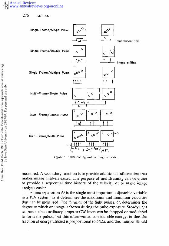
PULSE CODES Various pulse codes are illustrated in Figure 7, wherein theilluminating intensity Io is shown as a function of time, and the imagepatterns resulting from a single particle are shown in the frames. In thecase of single-frame recording the images from several pulses are super-imposed on a record that may consist of one frame of film or one electronicframe from a video-camera output. In either case, the total exposure ofthe frame is the integral of the exposures during the frame opening time,and once a frame is exposed the total exposure cannot be separatedinto its component exposures. Multiframing refers to cinematic film orsequences of video-image frames.

The primary function of the pulse code is to provide images at twoprecisely determined times, separated by At, from which Ax can be


Ann

u. R

ev. F

luid

Mec

h. 1

991.

23:2

61-3

04. D

ownl

oade

d fr

om a

rjou

rnal

s.an

nual

revi

ews.

org

by I

owa

Stat

e U

nive

rsity

on

03/1

7/07

. For

per

sona

l use

onl

y.


276 ADRIAN

Single Frame/Single Pulse

Single Frame/Double Pulse

Single Frame/Multiple Pulse

Multi-Frame/Single Pul~e

Multi-Frame/Double Pulse

Multi-Frame/Multi-Pulse

Figure 7

~ ~ Fluorescent tail

~&tt ~ t Image shifted

LLLL ft t

I Tf I I

, t,,,t , t t , t t

t~ t~ +Tt t~ +2Tt

Pulse-coding and framing methods.

measured. A secondary function is to provide additional information thatmakes image analysis easier. The purpose of multiframing can be eitherto provide a sequential time history of the velocity or to make imageanalysis easier.

The time separation At is the single most important adjustable variablein a PIV system, as it determines the maximum and minimum velocitiesthat can be measured. The duration of the light pulses, fit, determines thedegree to which an image is frozen during the pulse exposure. Steady lightsources such as ordinary lamps or CW lasers can be chopped or modulatedto form the pulses, but this often wastes considerable energy, in that thefraction of energy utilized is proportional to 6t/At, and this number should


Ann

u. R

ev. F

luid

Mec

h. 1

991.

23:2

61-3

04. D

ownl

oade

d fr

om a

rjou

rnal

s.an

nual

revi

ews.

org

by I

owa

Stat

e U

nive

rsity

on

03/1

7/07

. For

per

sona

l use

onl

y.



be small to avoid blurring of the image. It is more efficient to use pulsedsources such as flash lamps, spark discharges, or pulsed lasers.

Xenon flash lamps can emit several hundred joules in pulses as short as1 #s, but only a small fraction of this energy can be used to form a thin,high-quality light sheet owing to inherent limits on collimating light froman extended source. Spark discharges are narrower.

Pulsed lasers emit energy in collimated beams that can be formedefficiently into light sheets. Pulsed metal-vapor lasers produce green 10-nspulses repetitively at free-running frequencies in the 5-20 kHz range andenergies of order 10 mJ. These lasers are suitable for in-line holograms orfor photographing large particles in side-scatter. The time between pulsescan be lengthened by replacing the free-running frequency with an appro-priate pulse sequence for a brief interval, but very short time delays (e.g.less than 10 gs) are not readily available.

Pulsed ruby lasers produce 3 5 ms long fluorescence pulses of 699.3-nmlight that can be Q-switched two to four times during the fluorescencelifetime to produce sharp, 25-ns-long pulses with energies of order 1-10 J.The pulses can be separated by At’s as small as 1 #s and as large as about1 ms. To achieve time delays from a few milliseconds to several secondsin a double-pulsed mode, the laser rod can be pumped twice and Q-switched each time. Unfortunately, the time to recharge the capacitorbanks is long, so that ruby lasers typically do not fire a double pulse moreoften than once per minute.

Frequency doubled-pulsed Nd:Yag lasers fire 10-ns pulses at 532-nmlight repetitively at rates up to 50 Hz, and two lasers can be combined toproduce periodic trains of double pulses suitable for multiframing at 10-50 Hz with virtually any separation between the double pulses. Thesesystems are perhaps the most versatile of all of the available light sources.The lower pulse energy of the Nd : Yag laser relative to the ruby laser islargely compensated by the shorter wavelength, which leads to improvedscattering, thinner light sheets, and smaller images [cf Equation (14b)].

The energy requirements can be reduced considerably in special cir-cumstances. The effective intensity of a light sheet can be increased bysweeping a light beam to form the sheet, thereby concentrating the energyby a factor equal to the height of the light sheet divided by the height ofthe beam (Kawahashi & Hosoi 1989). This is useful in slowly changingflow fields. Vogel & Lauterborn (1988) achieved a substantially enhancedexposure using forward-scattered light. The object plane is fixed solely bythe depth of field. Binnington et al (1983) were able to use a 10-mW He-Ne laser by scattering from 15 to 40 #m TiO2-coated mica particles intoa close-up lens and using ASA 1600 film.

Photographic multiple framing can be done using autowinding cameras


Ann

u. R

ev. F

luid

Mec

h. 1

991.

23:2

61-3

04. D

ownl

oade

d fr

om a

rjou

rnal

s.an

nual

revi

ews.

org

by I

owa

Stat

e U

nive

rsity

on

03/1

7/07

. For

per

sona

l use

onl

y.


278 ADRIAN

at a few frames per second, cinematic cameras at 30 frames per second,and high-speed cameras at rates of up to several million frames per second.Standard video-imaging rates are 30 frames per second, but high-speedvideos with frame rates up to 80,000 per second are available. The veryhigh speed cameras, either photographic or videographic, produce a smallnumber of frames, so they cannot be used to film evolution of a flow fieldover a long period of time.

RECORDING MEDIA The principal difference between film and video isspatial resolution. Standard video tubes and video arrays offer about500 × 500 pixels, and high-resolution video arrays are available with2048 x 2048 pixels. They are currently expensive and relatively slow. Film,on the other hand, offers much higher resolution. A standard 35-mm frameof 300 lines per millimeter Kodak Technical Pan, for example, contains10,500 x 7500 pixels, and a 100 mmx 125 mm frame of portrait formatcontains 30,000 x 37,500 pixels. We shall see that this additional resolutionleads to approximately 10 times better spatial resolution and l0 timesbetter accuracy, relative to a standard video camera. Thus, film tends tobe used for high-resolution and wide dynamic velocity range measurementsof fluids, whereas video recording is suitable for lower resolution, loweraccuracy flow measurements, for higher accuracy measurements oversmaller fields of view, or for measurements of large particles in two-phaseflow. Undoubtedly, video resolution will continue to improve, and it is notunduly optimistic to anticipate that electronic photography may somedayoffer resolution comparable to chemical photography. In the meantime,researchers seeking the best performance will have to use photography.

Other two-dimensional recording media include photorefractive crystals(Collicott & Hesselink 1987) and thermoplastic films. Stereoscopic re-cording using several cameras and viewing directions and holographicrecording offer the possibility of making three-dimensional measurements.These media are discussed in a later section.

Resolution of Particle Motion

The accuracy of velocity measurements depends upon one’s ability todetermine the displacement of the particle, Ax, over a certain time intervalfrom measurements of the displacement of the image, AX. Assuming,for si~nplicity, one-dimensional motion and paraxial rccording, we haveAX = MAx = MuAt and

2 2~2AtO"u 1TAx

u2 - Ax2 + At2, (20)

where tr 2 denotes the mean square value of the error in measuring thesubscript quantity.


Ann

u. R

ev. F

luid

Mec

h. 1

991.

23:2

61-3

04. D

ownl

oade

d fr

om a

rjou

rnal

s.an

nual

revi

ews.

org

by I

owa

Stat

e U

nive

rsity

on

03/1

7/07

. For

per

sona

l use

onl

y.



The displacement Ax is uncertain owing to errors in locating the appro-priate reference points on the particle images used to mark the beginningand end of the displacement. The rcfcrence point is usually taken to be thecentroid of an image, but displacement of the centroid may not give thetrue particle displacement if the particle rotates, or deforms, or if its imagechanges in any other way during At. Errors in locating the ccntroid arisefrom the irregular shape of the image, finite resolution due to recording theimage on film of finite grain size or on a video detector array of finite pixelsize, and/or noise in the electronic readout of the video camera. For mostof these errors the rms value of Ax is proportional to the length of theimage given by the sum of the recorded image diameter de and the blurdue to particle translation during the pulse:

flax = c(dz + d~x/u2 + v261)¯ (21)

The uncertainty in At and the blur depend upon the light source, but thisis usually small unless the flow speed is very high. Assuming negligibletiming error, Adrian (1986a) has shown that the error in velocity measure-ment obeys a type of uncertainly principle, i.e.

0"uAXmax = CUmaxd,, (22)

wherein hx~,,x = Um,xAl is the spatial uncertainty in the location of thevelocity measurement, fixed by the maximum velocity range spanned bythe instrument. For given u .... the uncertainty is minimized by minimizingboth the image diameter de and the uncertainty in locating its centroid,represented by c.

LOW-IMAGE-DENSITY PIV

Principles

In the low-image-density limit, the mean number of particles per interroga-tion cell is small (N~ << 1). This concept can be applied to systems thatdo not employ an interrogation spot if we replace the volume of theinterrogation cell, rcd~Azo/4M2, with the volume lax] 3 defined by the par-ticle displacement, which is always appropriate because lax] must be lessthan AZo and/or ddM. The implications of low image density are threefold.Firstly, the number of images per unit volume to be processed is relativelysmall, so that one can afford, computationally, to perform many image-processing operations on each image individually. This is especially impor-tant in regard to image-pairing procedures, since the number of pairs isproportional to the square of the number of images. Secondly, there is alow probability of images overlapping in the same interrogation spot. The


Ann

u. R

ev. F

luid

Mec

h. 1

991.

23:2

61-3

04. D

ownl

oade

d fr

om a

rjou

rnal

s.an

nual

revi

ews.

org

by I

owa

Stat

e U

nive

rsity

on

03/1

7/07

. For

per

sona

l use

onl

y.


280 ADRIAN

probability of one particle in the interrogation volume is Nle-N’ ~ NI.Thirdly, the particles and hence the velocity measurements are randomlylocated. The mean spacing between nearest neighboring particles in thevolume is given by 0.55C-1/3, and the mean spacing of images in a lightsheet is (4CAzo)- i/2

Image processing is used both to improve the signal-to-noise ratio ofthe particle images relative to the background and to locate the images.Typical signal-enhancement steps begin with a histogram analysis of thegray levels and a noise-filtering operation to attenuate noise in the back-ground or to remove the noise pixels that can be identified by their lowlevels in the histograms. The contrast can be enhanced by subtracting amean level and anaplifying the bright pixels to the full-scale value ("his-togram slide and stretch"), and a threshold level can be set in order tolocate the edges of the particle images in terms of a maximum gray levelgradient criterion or a level found from the histogram analysis. The imagefield can be binarized by setting each pixel whose gray level exceeds thecertain threshold equal to one and zeroing all others. Following imageenhancement and edge detection, the centroid of each image can be located.The results of performing edge detection on some particle-streak imagesare shown in Figure 8. Various procedures are described by Dimotakis etal (1981), Hesselink (1988), Perkins & Hunt (1989), Adamczyk & (1988) and Kobayashi et al (1985). See also Pratt (1978).

Single-Frame Techniques

The simplest single-frame method is streak photography, which is ac-complished by time exposing particles in a light sheet over a long timeAt (Figures 7, 8). It can be viewed as a single, long-pulse technique or the limit of a large number of multiple pulses. It is an excellent methodfor quantitative visualization of two-dimensional flow fields, but in three-dimensional fields, foreshortened image streaks are created when particlesenter or leave the light sheet during the exposure, yielding low measure-ments.

Several important aspects of PIV can be illustrated by considering theprobability of making a successful measurement of velocity from a particlestreak. To be successful, the particle streak must not be truncated, and itmust not be obscured by overlapping with another streak. Truncation willnot occur if the particle lies in a sheet of thickness Azo- [wlAt, where w isthe out-of-plane velocity. The probability of not being truncated is given

by

Fo(wAt)= t l- IwlA~tAzo ’}wlAt < AzoI. (23)

0, IwlAt > AZoJ


Ann

u. R

ev. F

luid

Mec

h. 1

991.

23:2

61-3

04. D

ownl

oade

d fr

om a

rjou

rnal

s.an

nual

revi

ews.

org

by I

owa

Stat

e U

nive

rsity

on

03/1

7/07

. For

per

sona

l use

onl

y.


PARTICLE-IMAGING TECHNIQUES 28 l

2~.~

4c~

7~ ~9C~ 10~,

1~ 16 14% ~

Contours o£

(a) intersecting (b) pathline of (c) normalpathline adjacent particle pathline

Figure 8 Edge detection of particle streaks. (Top) Path lines of 18 fluorescent particles(reproduced with permission from Kobayashi & Yoshitake 1985); (bottom) digitization ofthe streak of a particle illuminated by a long pulse (reproduced with permission fromKobayashi et al 1985).

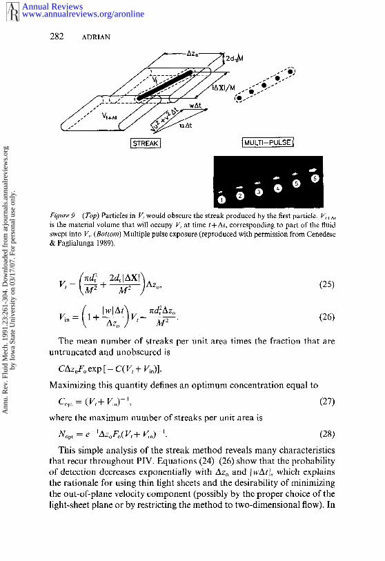
With reference to Figure 9. the particle streak will not be obscured ifthere is no other particle in the volume V, at time t and no other particleenters V, during the interval (t, t + At). The latter event is guaranteed if time t there are no particles in the volume Vi, = j’~, u- ds that is swept intoV, during (t, t + At). The probability of an untruncated, unobscured streakgiven the velocity u is then equal to

Prob {unobscured and untruncated its} = Foe-CV, e cv~o. (24)

If the fluid velocity is constant and the diameter of the particle image isd, the diameter and streak length projected back into the fluid are d~/Mand lAX I/M, respectively. It then follows that


Ann

u. R

ev. F

luid

Mec

h. 1

991.

23:2

61-3

04. D

ownl

oade

d fr

om a

rjou

rnal

s.an

nual

revi

ews.

org

by I

owa

Stat

e U

nive

rsity

on

03/1

7/07

. For

per

sona

l use

onl

y.


282 ADRIAN

~ I MULTI-PULSE I

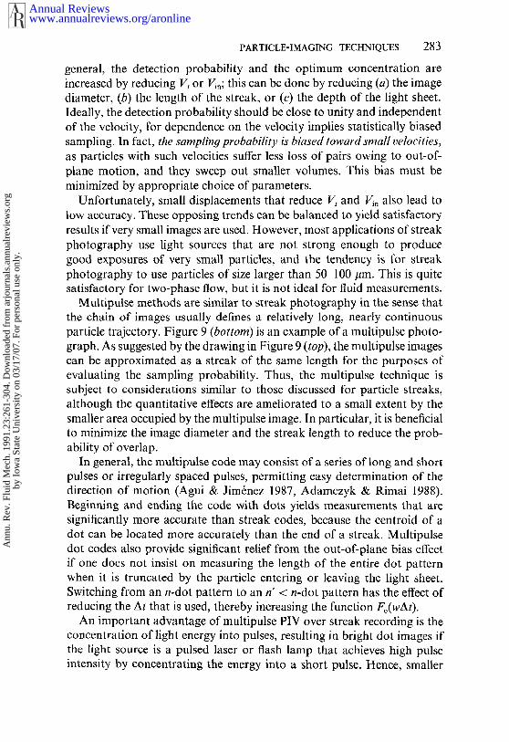
Figure 9 (Top) Particles in V, would obscure the streak produced by the first particle.is the material volume that will occupy V, at time t+At, corresponding to part of the fluidswept into V,. (Bottom) Multiple pulse exposure (reproduced with permission from Cenedese& Paglialunga 1989).

1(, = kM2 + -My -}zazo, (25)

~ = ~ + ~ ~ (~)

The mean number of streaks per unit area times the fraction that areuntruncated and unobscured is

C~zoFo exp [- C( V, + ~)].

Maximizing this quantity defines an optimum concentration equal to

Coot = (V,+ ~.) (27)

where the maximum number of streaks per unit area is

Nopt = e-~kzoFo(V,+ Vin)-1. (28)

This simple analysis of the streak method reveals many characteristicsthat recur throughout PIV. Equations (24)-(26) show that the probabilityof detection decreases exponentially with AZo and l wAll, which explainsthe rationale for using thin light sheets and the desirability of minimizingthe out-of-plane velocity component (possibly by the proper choice of thelight-sheet plane or by restricting the method to two-dimensional flow). In


Ann

u. R

ev. F

luid

Mec

h. 1

991.

23:2

61-3

04. D

ownl

oade

d fr

om a

rjou

rnal

s.an

nual

revi

ews.

org

by I

owa

Stat

e U

nive

rsity

on

03/1

7/07

. For

per

sona

l use

onl

y.



general, the detection probability and the optimum concentration areincreased by reducing Vt or Fin; this can be done by reducing (a) the imagediameter, (b) the length of the streak, or (c) the depth of the light sheet.Ideally, the detection probability should be close to unity and independentof the velocity, for dependence on the velocity implies statistically biasedsampling. In fact, the sampling probability is biased toward small velocities,as particles with such velocities suffer less loss of pairs owing to out-of-plane motion, and they sweep out smaller volumes. This bias must beminimized by appropriate choice of parameters.

Unfortunately, small displacements that reduce Vt and Vin also lead tolow accuracy. These opposing trends can be balanced to yield satisfactoryresults if very small images are used. However, most applications of streakphotography use light sources that are not strong enough to producegood exposures of very small particles, and the tendency is for streakphotography to use particles of size larger than 50-100/~m. This is quitesatisfactory for two-phase flow, but it is not ideal for fluid measurements.

Multipulse methods are similar to streak photography in the sense thatthe chain of images usually defines a relatively long, nearly continuousparticle trajectory. Figure 9 (bottom) is an example of a multipulse photo-graph. As suggested by the drawing in Figure 9 (top), the multipulse imagescan bc approximated as a streak of the same length for the purposes ofevaluating the sampling probability. Thus, the multipulse technique issubject to considerations similar to those discussed for particle streaks,although the quantitative effects are ameliorated to a small extent by thesmaller area occupied by the multipulse image. In particular, it is beneficialto minimize the image diameter and the streak length to reduce the prob-ability of overlap.

In general, the multipulse code may consist of a series of long and shortpulses or irregularly spaced pulses, permitting easy determination of thedirection of motion (Agui & Jim6nez 1987, Adamczyk & Rimai 1988).Beginning and ending the code with dots yields measurements that aresignificantly more accurate than streak codes, because the centroid of adot can be located more accurately than the end of a streak. Multipulsedot codes also provide significant relief from the out-of-plane bias effectif one does not insist on measuring the length of the entire dot patternwhen it is truncated by the particle entering or leaving the light sheet.Switching from an n-dot pattern to an n’ < n-dot pattern has the effect ofreducing the At that is used, thereby increasing the function Fo(wAt).

An important advantage of multipulse PIV over streak recording is theconcentration of light energy into pulses, resulting in bright dot images ifthe light source is a pulsed laser or flash lamp that achieves high pulseintensity by concentrating the energy into a short pulse. Hence, smaller


Ann

u. R

ev. F

luid

Mec

h. 1

991.

23:2

61-3

04. D

ownl

oade

d fr

om a

rjou

rnal

s.an

nual

revi

ews.

org

by I

owa

Stat

e U

nive

rsity

on

03/1

7/07

. For

per

sona

l use

onl

y.


284 ADRIAN

particles can be used, allowing more accuracy and higher data density.Chopped continuous sources do not enjoy this benefit; moreover, as theflow rate and the chopping rate increase, the pulse duration and hence theenergy per pulse decrease in inverse proportion, limiting these light sourcesto relatively slow flows and/or large particles unless the detector is verysensitive, such as for a video camera enhanced by a silicon intensifier tube(SIT).

An example of a velocity vector field in a water-channel flow measuredwith a four-pulse, stereo camera pair and 0.1-0.5 mm polystyrene particlesis shown in Figure 10 (Utami & Ueno 1984; cf also Utami & Ueno 1987).These results illustrate the randomness of the locations of the velocityvectors and the maximum data density that one typically expects with low-image-density PIV. Other examples of single-frame/multipulse PIV arefound in the work of Khalighi (1989), Agui & Jim6nez (1987), Braun et (1989), and Willis & Deardorff (1974).

Single-frame/double-pulse PIV has been studied in the low-image-den-sity limit by Landreth et al (1988). The use of only two pulses requiresspecial procedures to identify the direction of motion, and it makes thepairing of images more difficult. Adrian (1986b) proposed an image-shift-

o 0.00 ’1.00 8,00 12.00 |6-00 20-00 24.00 20.00X [CM)

Figure 10 Turbulent open-channel water-flow field measured by multipulse low-image-

density PIV (reproduced with permission from Utami & Ueno 1984).


Ann

u. R

ev. F

luid

Mec

h. 1

991.

23:2

61-3

04. D

ownl

oade

d fr

om a

rjou

rnal

s.an

nual

revi

ews.

org

by I

owa

Stat

e U

nive

rsity

on

03/1

7/07

. For

per

sona

l use

onl

y.



ing technique that resolves the directional ambiguity inherent in a two-dot record by optically shifting the image field between first and secondexposures to introduce an offset that exceeds the largest negative value ofone of the velocity components. In this way, the image displacementsare always positive, and negative particle displacements are inferred bysubtracting the imposed shift from the positive measurements. Shiftingcan be performed by photographing the fluid through a rotating mirror(Landreth et al 1988) or by using a birefringent crystal in front of thecamera to shift the image field when the polarization of the scattered lightis switched from the first pulse to the second pulse (Landreth & Adrian1988). Very rapid and precise shifting can be achieved with this technique.

Interrogation procedures for low-image-density PIV make use of thefact that the probability of images from different particles overlappingis low because the particle spacing is large compared with the particledisplacement. Landreth et al 0988) assumed that if an interrogation spotcontained two images, the images belonged to the same particle. Requiringexactly two images gave a data yield of about 0.1 velocity samples persquare millimeter when the interrogation spot was 1 mm2 and the imagedensity was 0.5. The pairing assumption failed in about 20% of the mea-sured vectors, resulting in bad measurements that had to be removedby postinterrogation processing of the vector field. The latter procedureremoved vectors that were substantially different from the locally averagedvector field. Following this approach, however, Landreth et al were unableto obtain fields containing over 2000 vectors in a turbulent-jet flow.

A somewhat different procedure is the nearest neighbor approach, inwhich each particle image is paired with its nearest neighboring image.Given an image from a particle in a light sheet, the probability that itsnearest neighbor is its second image equals the probability that it remainsin the light sheet at the time of the second exposure, Fo(WAt), times theprobability that there are no other particles in a cylinder of height AZoand radius x/72~v2At at time t, and that there are no other particles inthis same control volume at t + At. Assuming a Poisson distribution, theprobability can be shown to be

Prob {nearest image is true second image given u}

= Fo(wkt) exp [- (2- 0.53Fo) CAzog(U2 + v2)z~t:~]. (29)

To evaluate the unconditional probability, this equation must be averagedover the fluid velocities in the flow field. The successful detection rate perunit area is the number of images per unit area times this probability.

We see that, as in the case of the streak-image technique, the probabilityof obtaining a correct pair by this procedure can be made high by restricting


Ann

u. R

ev. F

luid

Mec

h. 1

991.

23:2

61-3

04. D

ownl

oade

d fr

om a

rjou

rnal

s.an

nual

revi

ews.

org

by I

owa

Stat

e U

nive

rsity

on

03/1

7/07

. For

per

sona

l use

onl

y.


286 ADRIAN

At, so that the out-of-plane displacement is a small fraction of Azo, and

the in-plane displacement ux/~v2At is small compared with the meanimage spacing (4CAzo)- 1/2. Small displacements give good spatial resolu-tion but poor accuracy, unless the diameters of the particle images aresmall. In Landreth et al (1988) the displacements were less than 0.5 and images less than 15 #m were obtained using a contact printingprocedure described by Pickering & Halliwell (1984). Accuracy was of theorder of 0.4-1% of the full-scale velocity.

Multiframe TechniquesThe simplest application of multiframing is to sample the velocity field ata periodic sequence of times with frame interval Tf, each sample consistingof a single, double, or multipulse exposure of the type discussed in theprevious section. In these methods the time between exposures (At) thatis used to measure the velocity is independent of the time between velocitysamples (Tr). This is advantageous because At can be selected accordingto the velocity and the requirements of spatial resolution, whereas Tr canbe chosen to follow the evolution of the flow, as determined by its inherenttime scales. Khalighi (1989) reports measurements of this type in which followed the development of the intake swirl in an engine using multipulseexposures recorded on successive frames of a video camera.

Multiframe/single-pulse methods are essentially conventional cine-matography and video recording of single exposures in each frame. Theadvantages of this approach are (a) the images of each exposure areisolated, eliminating confusion that results from superposing fields onsingle frames; (b) the particles can be tracked for long times; and (c) direction of motion is fully determined (Perkins & Hunt 1989). The prin-cipal disadvantage of this approach is that At is now constrained to beequal to Tf or an integral multiple, and this constraint confines measure-ments to low speeds if one uses standard 30-Hz video and cinematic framerates. If the maximum desirable displacement is 1 mm, the maximumallowable velocity is only 30 mm s t. Of course, higher speed cameras areavailable, but at very high speeds they produce a limited number of frames.

The reduced confusion that results from nonsuperimposcd imagesmakes it possible to achieve more reliable computer pairing of the images.Various procedures have been developed for tracking images from oneframe to the next. Frieden & Zoltani (1989) describe a nearest neighborsapproach, and Perkins & Hunt (1989) and Uemura et al (1989) detailautomated algorithms that involve cross correlation of groups coupledwith individual pairing. Both groups report processing times of order 10-40 s per video frame containing several tens or hundreds of particles usinga personal computer. Perkins & Hunt (1989) use results over many frames


Ann

u. R

ev. F

luid

Mec

h. 1

991.

23:2

61-3

04. D

ownl

oade

d fr

om a

rjou

rnal

s.an

nual

revi

ews.

org

by I

owa

Stat

e U

nive

rsity

on

03/1

7/07

. For

per

sona

l use

onl

y.



to track Lagrangian trajectories in two-phase flows. An example of thcirexperiment on the motion of large particles in a cylinder wake is shown inFigure 11. They estimate the error rate in matching particles to be 1 2%.Guezennec & Kiritsis (1989) describe a similar algorithm in which thevelocity field in a large region is estimated by cross correlation of theimages, and then the images in the first frame are projected onto the secondframe using this estimate. Pairing is done by a nearest neighbors criterionthat is obviously better than nearest neighbors without a priori dis-placement information because the displacement estimate reduces theallowable domain in which the second image can reside.

Three-dimensional, low-image-density PIV is usually performed withmultiframe recording, although there is no insurmountable reason why itcannot be done with single-frame exposures. Chang et al (1984) havedescribed pattern-matching techniques for stereo cinematic photographsof approximately 100 particles in a turbulent mixer, and more recentlyNishino et al (1989) have also automated the analysis of three videoviews of 280-#m particles in decaying turbulence in water using a 10-Hzvideoframe rate. The observed volume is 5 cm x 5 cm x 5 cm, and theywere able to measure 100 vectors out of approximately 600 images recordedin each frame. The point positions indicated by the cameras were calibrated

.." ..w"’,,,:... "/, "¯

....: j, "": "-’’" "-:::" . ’~,:’,,"x"’-. "% ~’~ " " "’" ~’-¯ -" ,. -,,, \’- ..,~. "x.~--’---.

~ . ".. - .,.. --....."-."’-.... \ _

..... "---4,_."7-- -

Figure 11 Trajectories of particles in a cylinder wake measured by ~nultiframe/single-pulserecording and image tracking (reproduced with permission from Perkins & Hunt 1989),


Ann

u. R

ev. F

luid

Mec

h. 1

991.

23:2

61-3

04. D

ownl

oade

d fr

om a

rjou

rnal

s.an

nual

revi

ews.

org

by I

owa

Stat

e U

nive

rsity

on

03/1

7/07

. For

per

sona

l use

onl

y.


288 ADRIAN

and fit to a representation developed by Murai et al (1980) for cameraswith arbitrary orientation and lens distortion. Related work is reportedby Racca & Dewey (1988), who use orthogonal views, and Kent & Eaton(1982).

As noted earlier, stereoscopic photographic recording of three-dimen-sional volumes requires large depth of field, which in turn requires lowphotographic resolution [cf Equations (5) and (7)]. The relatively largeparticles used by Nishino et al (1989) are symptomatic of these require-ments and are consistent with the resolution provided by a video camera.

Higher resolution in three-dimensional volumes can be achieved byusing holographic recording because the depth of the hologram is muchlarger than the depth of field of a lens. Further, the point response of ahologram is inversely proportional to the size of the holographic plate,and the size is often many times larger than the feasible aperture of a lens,yielding improved resolution (Akbari & Bjelkhagen 1986).

High-speed holographic/cinematic recordings have been proposed byWeinstein et al (1985) using a system in which a copper-vapor laser oper-ates at less than 2 kHz and illuminates 40-/~m particles in water to formsequences of in-line holograms that are recorded on a 35-mm high-speedfilm transport. Three-dimensional particle positions are located accuratelyby using two orthogonal holographic views. The particle-image fields in agiven frame are reconstructed and viewed with a video camera mountedon an XYZ controller to scan the fields and locate the particle centroids.Tracking is performed from frame to frame. It is understood that theresults of this project will be forthcoming shortly.

Haussmann & Lauterborn (1980) and Zarschizky & Lauterborn (1983)have also used high-speed holographic techniques to record the fluid fieldsand motions of bubbles in cavitating flows. Rates of 67,700 holograms persecond were achieved.

HIGH-IMAGE-DENSITY PIV

Principles

High-image-density PIV uses particle concentrations large enough toensure that every interrogation spot contains many images. In the limitN~ >> 1 the probability of finding no particles in a spot [given by exp(- N~)]is very small. In practice, values ofN~ > 5-10 produce asymptotically largebehavior.

High-image-density PIV is usually performed with single-frame record-ing on photographic film for the purposes of providing maximum resolu-tion in space and velocity. The particle images must be small, typically oforder 10-25 #m, to avoid filling the interrogation spot whose size is less


Ann

u. R

ev. F

luid

Mec

h. 1

991.

23:2

61-3

04. D

ownl

oade

d fr

om a

rjou

rnal

s.an

nual

revi

ews.

org

by I

owa

Stat

e U

nive

rsity

on

03/1

7/07

. For

per

sona

l use

onl

y.



than a few millimeters, and to give accurate measurements when thedisplacements are small. Typical displacements are 10/~m to a few milli-meters. The field of view is often a 25 mmx 35 mm frame, but 100mm × 125 mm frames containing several tens of thousands of interroga-tion spots are also used. A section of a single-frame/double-pulsed high-image-density photograph is shown in Figure 12.

Multiple-exposed single frames are preferred over single-exposed multi-frames because the inaccuracy of registering separate frames over a largefield of view can cause severe errors. For example, 0.1% shrinkage of a100-mm frame produces spurious displacement of images in that framerelative to those in another fraine as large as 100/~m. This can be a largefraction of the total displacement. On the other hand, multiple exposureson the same film frame are automatically registered with respect to eachother, and any registration error refers to the location of the measurement,not the displacement.

Figure 12 Single-frame/double-pulsed photograph of 5-~m A1203 spheres in a turbulentwater channel. Mean flow is from left to right.


Ann

u. R

ev. F

luid

Mec

h. 1

991.

23:2

61-3

04. D

ownl

oade

d fr

om a

rjou

rnal

s.an

nual

revi

ews.

org

by I

owa

Stat

e U

nive

rsity

on

03/1

7/07

. For

per

sona

l use

onl

y.


290 ADRIAN

Exposures may be double pulses or multiple pulses, but unless otherwise stated, the following discussions pertain to the double-pulsed case.

The primary consequences of high image density are that almost every interrogation cell contains enough particles to yield a measurement, and that the large number of images makes it difficult to track individual particles. The types of interrogation-spot images that must be processed are illustrated in Figure 13. The left-hand column contains images of 1 mm x 1 mm interrogation spots located at different points in an impinging vertical jet flow. Figure 13a is from a spot located in a region of nearly

Figure 13 Sample interrogations of 1 mm x 1 mm spots digitized with a 256 x 256 video array. (a,d, g, j ) Image fields of the interrogation spots; (b,e,h,k) fringe patterns resulting from Fourier transforms of the image fields; (c ,Ai , l ) correlation patterns resulting from Fourier transforms of the fringe patterns (reproduced with permission from Landreth & Adrian 1989).


Ann

u. R

ev. F

luid

Mec

h. 1

991.

23:2

61-3

04. D

ownl

oade

d fr

om a

rjou

rnal

s.an

nual

revi

ews.

org

by I

owa

Stat

e U

nive

rsity

on

03/1

7/07

. For

per

sona

l use

onl

y.



uniform, slow vertical velocity, whereas the spot in Figure 13d is from aregion of larger vertical velocity. Figure 13g is from the shear-layer regionof the jet, where the horizontal gradient of the vertical velocity was large,and Figure 13j is from a corner of the photograph, where the lens distortionproduced very poor images. The image density in these spots is aboutN~ ~- 20.

Knowing that the velocity is vertical, it is easy for one to see the pairsof images in Figure 13a, but not so easy in Figure 13d. The gradient inFigure 139 makes pairing by eye quite difficult, and the poor qualityof images in Figure 13j makes it impossible. The challenge of imageinterrogation is to design computer algorithms that will measure the dis-placements of images in such spots accurately, reliably, and with a mini-mum amount of human intervention.

The methods of interrogation that are currently in use are primarilystatistical approaches that probabilistically infer the proper pairings andmeasure the average displacement of the group of particles in the interroga-tion cell. The speed of interrogating a spot is an important issue, as eachphotograph contains thousands of spots. Several of the methods that areused are discussed next.

Interrogation Techniques

As shown in Figure 4, interrogation of a photograph begins by illuminatingan interrogation spot with a beam of intensity I~(X-X0, where X~ is thecenter of the spot. The interrogation spot intensity is given by

I(X) = I,(X- X~)z(X), (30)

where z(X) is the intensity transmissivity of the photographic image.If the images are recorded on a video frame instead of a photograph,

the interrogation spot can be defined digitally by multiplying the data inthe frame array by a window function whose shape corresponds to lvSince the parallels between video recording and photographic recordingare generally obvious (except for noise effects, such as film grain andelectronics readout noise), we shall discuss interrogation in terms of photo-graphic recording only.

DIRECT AUTOCORRELATION The autocorrelation of I(X) is given

R(s) = I( X)I(X+s)dX, (31)dspot

where s is a two-dimensional displacement vector. The third column inFigure 13 shows R(s) for each of the interrogation spots in the first column.Where s = 0, there is a strong self-correlation peak Rp, corresponding to


Ann

u. R

ev. F

luid

Mec

h. 1

991.

23:2

61-3

04. D

ownl

oade

d fr

om a

rjou

rnal

s.an

nual

revi

ews.

org

by I

owa

Stat

e U

nive

rsity

on

03/1

7/07

. For

per

sona

l use

onl

y.


292 ADRIAN

each image correlating with itself. Where s equals the mean displacement,there is a second peak RD+, called the positive displacement peak, thatcorresponds to first images correlating with second images. An identicalpeak RD occurs at the negative value of the mean displacement, cor-responding to second images correlating with first images. In addition tothe self-correlation peak (which conveniently defines the origin) and thetwo strong displacement peaks, there are a number of noise peaks resultingfrom random overlap of particle images in the I(X)I(X ÷ s) product.

The velocity is determined by locating thc ccntroid of the tallest peakin the correlation plane (other than the self-correlation peak). If the tallestpeak is the positive displacement peak with centroid /~D+, the velocity isestimated from

I~) -- I~D+/MAt. (32)

The measured ccntroid contains, of course, a random component thatdepends upon the distribution of particles and the correlation noise. It hasbeen shown (Adrian 1988) that the expected value of the centroidal velocityestimation is a volume average of the velocity in the interrogation cell, i.e.

fu(x, t) Wdx

(/~1 lu) , (33)

where W is a weighting function given by

W = lo,(x)lo2(X uAt)l,(Mx-- X,)li(Mx + MuAt- X,). (34)

Here Io~ and 1o2 are the intensities of the first and second light sheets. Thedependence of W on u defines a measurement volume whose size is biasedtoward low-velocity particles that have less chance of leaving the lightsheet and/or the interrogation spot. This velocity bias is zero if the velocityis uniform, and it is small if the velocity variation across the measurementregion is small, i.e. if the spatial resolution is adequate.

The strength of the displacement correlation peak.is proportional to thenumber of particle-image pairs in the interrogation cell. This number isproportional to NI, decreased by the fraction of second images that leavethe cell due to out-of-plane motions and by the fraction lost by in-planemotion. For uniform flow with velocity u, the mean of the displacementcorrelation evaluated at its peak value is (Keane & Adrian 1990)

½Rp(O)Fo(wAt) exp [- 4[MuAtlZ/(d~ + d~2)],

where Fo represents the out-of-plane loss of pairs, and the exponential


Ann

u. R

ev. F

luid

Mec

h. 1

991.

23:2

61-3

04. D

ownl

oade

d fr

om a

rjou

rnal

s.an

nual

revi

ews.

org

by I

owa

Stat

e U

nive

rsity

on

03/1

7/07

. For

per

sona

l use

onl

y.



function represents the in-plane loss of pairs. [Note the similarities withEquation (29).] Hence, the large velocities reduce the amplitude of thesignal peak.

If one of the noise peaks exceeds the positive displacement peak, it willbe identified incorrectly as the signal peak, and an invalid measurementresults. To reduce the probability of invalid measurements, one can requirethat the ratio of the tallest peak (excluding Rp) to the next tallest exceedsa prescribed detection threshold. One can also restrict the search for thetallest peak to a region in the s-plane in which the vector is expected to belocated, on the basis of consistency with neighboring measurements, orone can accept invalid measurements during interrogation and clip themout of the vector data file in a postinterrogation procedure that compareseach vector with its neighboring vectors (Landreth & Adrian 1989). At thesame time, the second, third, and fourth tallest peaks can be evaluated tosee if they would yield vectors more consistent with the neighboring field.

In any measurement procedure, the displacement correlation peakbecomes smaller and less likely to be detected as the velocity increases. Werefer to this bias against high velocities as velocity bias. In low-image-density PIV, it biases all measurements. In high-image-density PIV, ve-locity bias is much less severe because the loss of image pairs does not causea measurement failure if the number of remaining pairs is large enough.Thus, the fraction of successful measurements asymptotically approaches100% as N~ becomes large and [AXI/d~ is made small.

Theoretical analysis and extensive numerical simulations (Keane Adrian 1990) show that the performance of the double-pulsed auto-correlation technique is optimized by the following approximate criteria:

N[ > 10-20,

N/~U2-t-VzAt < ~dl/M,

wAt < ~Azo,

IAul/lul < 0.2,where I Aul is the velocity variation over the measuring volume due to localgradients. By satisfying these constraints, it is possible to make validmeasurements in over 90-95% of the interrogation spots with small biaserrors.

The use of multiple pulses separated by At improves the strength of thcdisplacement correlation by increasing the number of correlated pairs ofimages. For example, a four-pulse single exposure containing N[ particles,none of which leave the volume, would produce a self-correlation peak ofheight 4N[, a first correlation peak at s = MuAt that is 3N~ high, a second


Ann

u. R

ev. F

luid

Mec

h. 1

991.

23:2

61-3

04. D

ownl

oade

d fr

om a

rjou

rnal

s.an

nual

revi

ews.

org

by I

owa

Stat

e U

nive

rsity

on

03/1

7/07

. For

per

sona

l use

onl

y.


294 ADRIAN

peak at 2MuAt that is 2N~ high, and a third peak at 3MuAt that is N~high. The performance is much the same as for a double-pulse image from3N~ particles using the same At. If the four-pulse exposure were obtainedby reducing At by three to maintain the same total distance from beginningto end, then the first correlation peak would be more detectable but lessaccurate.

DIRECT CROSS CORRELATrON The loss of pairs due to in-plane motion outof the interrogation spot can be eliminated by performing cross-correlationbetween first images in a small, first interrogation window and secondimages in a larger, second interrogation window. The procedure is verysimilar to that described by Landreth et al (1988), except that searchingthe second window for a second image is replaced by cross-correlating allimages. The second window is chosen on the basis of a priori knowledgeabout the flow field, such as a predominant ~nean flow, an imposed imageshift, or an estimate of the local flow direction based on neighboringvectors. Similarly, a priori knowledge of the out-of-plane cofnponent canbe used to locate the second light sheet in a plane that will capture mostof the second images, as in Lee et al (1989). Cross correlating images in first interrogation cell with those in a second cell will increase the strengthof the correlation peak and thereby increase the probability of makingvalid measurements. More work is needed in this area.

YouyG’s F~IYG~S The Young’s fringe method has been used more widelythan any other technique for interrogation of high-image-density photo-graphs. As shown in Figure 4 (/)ottom) a lens is used to perform a two-dimensional Fourier transform of the lightwave from the interrogationspot, and the intensity of the Fourier transform is measured a distance Lfrom the lens. The lens performs an accurate Fourier transform of thephase and the amplitude of the lightwave if it is located one focal lengthfrom the film and if the fringe plane is one focal length from the lens(Goodman 1968). Physically, each image acts as a point source whose raysare collimated by the lens into a plane wave propagating at a small angleto the optic axis of the lens. Each pair of images produces a pair ofmutually inclined plane waves that interfere to form a Young’s fringepattern oriented perpendicular to the displacement vector between theimages. The randomly located image pairs produce fringes with randomorientations and spacings that superpose to form a random speckle pat-tern. The pairs that are separated by the same displacement vector formidentical fringes that reinforce each other, thereby creating a dominantpattern.

The fringe pattern in Figure 13/) is typical of a pattern from severaluniformly spaced pairs. In Figure 13e the small fringe spacing caused by


Ann

u. R

ev. F

luid

Mec

h. 1

991.

23:2

61-3

04. D

ownl

oade

d fr

om a

rjou

rnal

s.an

nual

revi

ews.

org

by I

owa

Stat

e U

nive

rsity

on

03/1

7/07

. For

per

sona

l use

onl

y.



the large pair spacing makes the fringes difficult to see. The fringes arealso difficult to see in Figure 13h owing to velocity gradients creatingfringes with variable spacing. In Figure 13k the poor image quality alsoobscures the fringes.

Interrogating the fringes involves determining their orientation and theirspacing. Numerous one-dimensional techniques have been proposed (cfMeynart 1983c, Kaufman et al 1980, Ineichen et al 1980, Lourenco &Krothapalli 1988). These methods form one-dimensional samples, eitherby sampling along lines across the fringe pattern or by compressing thetwo-dimensional Young’s fringe pattern into a one-dimensional arrayusing cylindrical lenses or integration. The one-dimensional arrays can beanalyzed quickly by Fourier transform or by fringe counting. A variationon the one-dimensional theme forms one-dimensional fringes by using acylindrical lens to perform a one-dimensional Fourier transform (Collicott& Hesselink 1986).

The most powerful method of analyzing Young’s fringes is the two-dimensional Fourier transformation of the fringe-intensity distribution.The transformation can be performed digitally, in which case a videocamera digitizes the Young’s fringes and a fast Fourier transform (FFT)of the digitized array is then calculated by a computer (Adrian 1986a,Huntley 1986a). It can also be done optically, as is discussed in the nextsection. The Fourier transform of the fringe intensity equals the Fouriertranstbrm of the product of the Fourier transform of the amplitude imagefield multiplied by the complex conjugate of the Fourier transform of theamplitude of the image field. From the convolution theorem, the Fouriertransform of the product is equal to the convolution of the Fourier trans-forms, or, in other words, the convolution of the amplitude of the inter-rogation-spot image field. As shown in Keane & Adrian (1990), this is onlyslightly different from the convolution of the intensity of the interrogation-spot image field, so that the Fourier transform of the Young’s fringepattern can be analyzed using the same procedures that have beendescribed for the analysis of the two-dimensional correlation function. Inparticular, the FFT of the fringe intensity will yield a convolution functionthat contains a self-correlation peak, positive and negative displacementpeaks, and noise peaks.

The advantage of the Young’s fringe method is that it performs oneFourier transformation optically, with no cost to the total processing time.This is a significant savings that can increase the processing speed by afactor of two. For example, the interrogation system used by Landreth &Adrian (1990) employs a Numcrix 432 array processor operating at Mflop to perform a 256 × 256 FFT computation in 190 ms. In this study,direct digital correlations were computed by digitizing each image spot


Ann

u. R

ev. F

luid

Mec

h. 1

991.

23:2

61-3

04. D

ownl

oade

d fr

om a

rjou

rnal

s.an

nual

revi

ews.

org

by I

owa

Stat

e U

nive

rsity

on

03/1

7/07

. For

per

sona

l use

onl

y.


296 ADRIAN

onto a 256 x 256 array and digitally performing one real-to-complex FFT,computing the modulus squared of each element in the array and thenperforming an inverse real-to-complex FFT taking advantage ofsymmetry. Including the search time for the four tallest peaks, the totaltime required was 0.45 s per interrogation spot. In comparison, by usinga lens in a Young’s fringe system to perform the first FFT, the computationtime is reduced to 0.3 s per spot.

The advantage of direct imaging is that image processing can beperformed on the particle images, including signal enhancement, centroid-ing, and particle sizing.

Huntley (1989) has compared four methods of Young’s fringe analysis:two-dimensional Fourier transform, two-dimensional Walsh transform(Huntley 1986b), one-dimensional integration (Robinson 1983), and dimensional autocorrelation (Meynart 1983a). He finds that the two-dimensional Fourier transform gives the lowest error.

Malyak & Thompson (1984) have described a method of formingYoung’s fringes from recordings of in-line holograms.

OPTICAL CORRELATION The two-dimensional correlation function of aninterrogation spot can be formed optically by replacing the two digitalFFT operations with optical Fourier transformations. The generic opticalcorrelator consists of a lens that Fourier transforms the amplitude of theinterrogation-spot image, a device that forms the modulus squared, and asecond lens that Fourier transforms the modulus squared (cf Goodman1968). The system is the same as a Young’s fringe system up to the fringeplane, at which point the intensity of the fringes must be written onto anoptical device that transmits a coherent wave whose amplitude is pro-portional to the fringe intensity. The transmitted wave is Fourier trans-formed by a lens to form an optical field whose amplitude is proportionalto the correlation function. The intensity of this field is digitized by a videocamera, and the usual peak-detection and centroid calculations are donedigitally.

Interestingly, the most difficult step in coherent optical correlation isforming a coherent field whose amplitude is proportional to the modulussquared of the first Fourier transform, i.e. the intensity of the Young’sfringe pattern. This can be done by photographing the Young’s fringesand illuminating the developed photograph coherently, but to develop aphotograph for each interrogation spot is clearly too awkward. Arnold &Hinsch (1988) have made this process more feasible by using holographic-imaging elements to form many interrogation spots that can be photo-graphed simultaneously.

Photorefractive crystals such as bismuth silicon oxide (BSO) are capable


Ann

u. R

ev. F

luid

Mec

h. 1

991.

23:2

61-3

04. D

ownl

oade

d fr

om a

rjou

rnal

s.an

nual

revi

ews.

org

by I

owa

Stat

e U

nive

rsity

on

03/1

7/07

. For

per

sona

l use

onl

y.



of recording an intensity field in the form of a refractive-index variationthat can be subscquently erased by changing the electric field applied tothe crystal. Coupland & Halliwell (1988) describe a system in which hologram of the interrogation spot is recorded in a BSO crystal using anoff-axis reference beam. When the reference beam is removed, the crystalphase modulates the incident wave to produce a transmitted wave whoseamplitude is proportional to the fringe intensity. BSO crystals respondslowly at moderate recording energies. Coupland & Halliwell (1988) report1 s response at 10 mW cm-2. However, Gheen & Cheng (1988) havedemonstrated 1000 times faster response in GaAs:Cr photorefractivecompound semiconductors.

Another approach to optical correlation uses a video camera to digitizethe intensity of the Young’s fringe pattern and then writes the intensitypattern to a medium whose amplitude transmittance is proportional to thewrite signal. Farrell & Goetsch (1989) have demonstrated the feasibilityof using a liquid-crystal TV screcn for this purpose, while Kompenhans etal (1989) have done similar feasibility experiments with a Faraday-effectspatial light modulator.

Spatial light modulators and photorefractive crystals currently do nothave very fast response times, but these times can be expected to decrease.Ultimately, the speed of optical interrogation methods may be limited bythe time required to write the video digitization of the correlation functioninto a peak-search device and by the peak-search time itself.

The choice between analog optical methods and digital methods is notclear; it will ultimately depend on future technological developments inoptical and semiconductor computing. For example, very fast digital-processor boards for two-dimensional FFT calculations are certain tobecome available, and even using available array processors such as theNumerix device described above, it has been possible to process 3000vectors per minute with good accuracy by reducing the interrogation-spotpixel resolution to 32 × 32. At this rate, a grid of 25 × 35 vectors on astandard 35-ram frame of film can be analyzed in less than 20 s.

Applications

High-image-density PIV has been used to study many flows. Applicationshave been mainly in water owing to the ease of seeding liquids withscattering particles, but several successful experiments have been per-formed in airflows, including some in difficult environments. Water-flowstudies include the multipulse work of Lourenco & Krothapalli (1987,1988) on wakes and airfoils, the turbulent thermal-convection experimentsof Meynart et al (1987) and Arroyo et al (1988), the impinging wall-jetstudy of Landreth & Adrian (1990), and studies of wave motion by G~irtner


Ann

u. R

ev. F

luid

Mec

h. 1

991.

23:2

61-3

04. D

ownl

oade

d fr

om a

rjou

rnal

s.an

nual

revi

ews.

org

by I

owa

Stat

e U

nive

rsity

on

03/1

7/07

. For

per

sona

l use

onl

y.


298 ADRIAN

et al (1986). Kompenhans & H6cker (1988) have been able to make high-image-density PIV measurements in a 360 m s ~ air jet.

A sample velocity field from a recent turbulent water-channel flow studyby Liu et al (1990) is shown in Figure 14. In this experiment a double-pulsed ruby laser with 2 J per pulse illuminated 5-/tm diameter A1203spheres whose image density was carefully adjusted to give 10-20 particlesper interrogation spot. The measurement volume dimensions were 1.0mm x 0.3 mm x 0.8 mm in the x-, y-, and z-directions, respectively,corresponding to 7.5 x 2.25 x 6.0 in terms of viscous wall units. Therectangular shape of the interrogation cell was chosen to improve theprobability of finding pairs in a flow with a strong x-component. (Theroot-mean-square velocity fluctuation on the centerline of the channel isonly 4% of the mean flow.) Photographs like that in Figure 12 wereinterrogated on a 0.5-mm grid by two-dimensional FFT of the Young’sfringe pattern. The flow field contains 12,000 vectors, each accurate to

y+ y(mm)

3001 40-270-

240-30-

210-

180,

150- 20-

120-

90-

60-

30- 0-

O-0 10 20 30 40 50 x(mm)

~ ~ ~0 1~0 2~0 ~0 ~0 4~0 ~.Figure 14 Fluctuating velocity field in turbulent channel flow at a Reynolds number of2872 based on the hal~channel height. The fluid is water (reproduced with permission fromLiu et al 1990).


Ann

u. R

ev. F

luid

Mec

h. 1

991.

23:2

61-3

04. D

ownl

oade

d fr

om a

rjou

rnal

s.an

nual

revi

ews.

org

by I

owa

Stat

e U

nive

rsity

on

03/1

7/07

. For

per

sona

l use

onl

y.



about 1% of the full-scale mean velocity. (The local mean velocity hasbeen subtracted to obtain the fluctuating velocity vectors in Figure 14.)

The density of data in Figure 14 is high enough to permit differentiationto calculate the out-of-plane component of vorticity. The vorticity con-tours in Figure 15 correspond to the velocity field in Figure 16. Note theconcentrations of vorticity in shear layers close to the walls. Statistics ofthe turbulent flow have been calculated by averaging along lines of constanty and ensemble averaging over 11 photographs. Mean-velocity profilescalculated in this way are plotted in the usual wall variables U÷ and y+ inFigure 16 and compared with LDV measurements and direct numericalsimulations. The agreement is encouraging.

High-quality airflow measurements can be performed by PIV if care istaken to ensure adequate concentrations of the appropriate scatteringparticles. Measurements of grid turbulence in a large, relatively high-speedwind tunnel have been reported by H6cker & Kompenhans (1989). Theyused 1-/~m oil droplets. Reuss et al (1989) performed measurements in motored research model of an internal combustion engine using the reac-tion of TIC14 with water vapor to produce TiO2 particles in the 1-2 #mrange.

In addition to its applications to turbulent flows, PIV is very useful inthe study of flows with complex geometries. Paone et al (1989) have,for example, measured fields in the passageways of a centrifugal pumpimpeller.

Fi#ure 15 Contours of the z-component of vorticity found by differentiating the vector fieldin Figure 14 (reproduced with permission from Liu et al 1990).


Ann

u. R

ev. F

luid

Mec

h. 1

991.

23:2

61-3

04. D

ownl

oade

d fr

om a

rjou

rnal

s.an

nual

revi

ews.

org

by I

owa

Stat

e U

nive

rsity

on

03/1

7/07

. For

per

sona

l use

onl

y.


300 ADRIAN

20 ¯

÷~ 10

¯ Re - 2872 (PIN

~ Re - 2e00 (DNS)

+ Re

.1 1 10 100 1000It’+

Streamwise mean velocities

Figure 16 Mean-velocity profile in the turbulent channel flow calculated from an ensembleof ! 1 PIV photographs. The comparison is with LDV data and direct numerical simulations(reproduced with permission from Liu et al 1990).

CONCLUDING REMARKS

Particle-image velocimetry has developed rapidly during the last decade.It is now clear that the basic two-dimensional technique is capable ofproviding accurate, high-quality measurements of instantaneous fields ina variety of laboratory-scale flows of gases and liquids spanning the rangefrom millimeters per second to several hundred meters per second.Interrogation methods depend upon the image density, with the greatestdemands for interrogation time coming from high-density photographs.The computation time required to process a photograph is now reasonableusing appropriate laboratory computers, and the computation needed toprocess a single low-image-density video frame can be handled by relativelysmall computers. As the analysis of the images becomes less demanding,one can anticipate extensions of the technique to measurements involvinghundreds or even thousands of frames of data. In particular, cinematicrecording of vector fields, stereographic recording, and holographic re-cording are generalizations that will become more com~non as processingtimes decreased.


Ann

u. R

ev. F

luid

Mec

h. 1

991.

23:2

61-3

04. D

ownl

oade

d fr

om a

rjou

rnal

s.an

nual

revi

ews.

org

by I

owa

Stat

e U

nive

rsity

on

03/1

7/07

. For

per

sona

l use

onl

y.



Interrogation techniques will continue to evolve, although the two-dimensional correlation and two-dimensional FFT techniques are alreadyso good that major improvements in the data yield and the data reliabilityarc not to be expected. Work is needed to relate measurements to theactual flow field in greater detail and to develop methods of interrogatingregions of very rapid velocity variation with high reliability.

One of the most welcome capabilities offered by PIV is the measurementof vorticity and rate-of-strain fields. These quantities are as fundamentalto fluid mechanics as the velocity field itself, but they have been largelyabsent from the experimentalist’s vocabulary owing to the difficulties inmeasuring derivative quantities even on a point-wise basis.

ACKNOWLEDGMENTS

This article was prepared with support from the National Science Foun-

dation under Grant ATM 8920605 and the Office of Naval Research underContract N0001490J1415 and Argonne/DOE Contract 82862403.

Literature Cited

Adamczyk, A. A., Rimai, L. 1988. 2-Di-mensional particle tracking velocimetry(PTV): technique and image processingalgorithms. Exp. Fluids 6:373-80

Adrian, R. J. 1983. Laser velocimetry. InFluid Mechanics Measurements, ed. R.Goldstein, pp. 155-244. Washington, DC:Hemisphere. 630 pp.

Adrian, R. J. 1984. Scattering particlecharacteristics and their effect on pulsedlaser measurements of fluid flow: specklevelocimetry vs. particle image velocimetry.Appl. Opt. 23:1690-91

Adrian, R. J. 1986a. Multi-point opticalmeasurements of simultaneous vectors inunsteady flow--a review. Int. J. HeatFIuM Flow 7:12745

Adrian, R. J. 1986b. Image shifting tech-nique to resolve directional ambiguity indouble-pulsed velocimetry. Appl. Opt.25(21): 3855-58

Adrian, R. J. 1988. Statistical properties ofparticle image velocimetry measurementsin turbulent flow. In Laser Anemometry inFluid Mechanics--Ill, ed. R. Adrian, T.Asanuma, D. Durgo, F. Durst, J. White-law, pp. 115-29. Lisbon: Ladoan-lnst.Super. Tec. 541 pp.

Adrian, R. J., Yao, C.-S. 1984. Developmentof pulsed laser velocimetry (PLV) formeasurement of turbulent flow. In Proc.Symp. Turbul., ed. X. Reed, G. Patterson,J. Zakin, pp. 170-86. Rolla: Univ. Mo.380 pp.

Adrian, R. J., Yao, C.-S. 1985, Pulsed lasertechnique application to liquid and gase-ous flows and the scattering power of seedmaterials. Appl. Opt. 24:44-52

Adrian, R. J., Yao, C.-S. 1987. Power spectraof fluid velocities measured by laserDoppler velocimetry. Exp. Fluid¢ 5: 17-28

Agui, J. C., Jim6nez, J. 1987. On the per-formance of particle tracking. J. FluidMech. 185:447~8

Akbari, H., Bjelkhagen, H. I. 1986. Ho-lography in 15-foot bubble chamber atFermilab. Proc. Soc. Photo-Opt. lnstrum.En9. 615:7-12

Archbold, E., Ennos, A. E. 1972. Dis-placement measurements from doubleexposure laser photographs. Opt. Acta 19:253-71

Arnold, W., Hinsch, K. 1988. Purely opticalparallel processing in particle image vel-ocimetry and the study of flow structures.Proc. Conf Opt. Methods in Flow andPart. Diagnostics, ICALEO ’88, Orlando,Fla: Laser Inst. Am. (Abstr.)

Arroyo, M. P., Yonte, T., Quintanilla, M.,Savirdn, J. M. 1988. See Chiang & Reid1988, pp. 295-316

Barker, D. B., Fourney, M. E. 1977. Measur-ing fluid velocities with speckle patterns.Opt. Lett, 1:135-37

Binnington, R. J., Troup, G. J., Boger, D.V. 1983. A low cost laser-speckle photo-graphic technique for velocity measure-


Ann

u. R

ev. F

luid

Mec

h. 1

991.

23:2

61-3

04. D

ownl

oade

d fr

om a

rjou

rnal

s.an

nual

revi

ews.

org

by I

owa

Stat

e U

nive

rsity

on

03/1

7/07

. For

per

sona

l use

onl

y.

302 ADRIAN

ment in slow flows. J. Non-NewtonianFluidMech. 12:255 67

Braun, M. J., Canacci, V. A., Russell, L.,Hendricks, R. C. 1989. A laser based com-puter aided non-intrusive technique forfull field flow characterization in macro-scopic curved channels. In Flow Visual-ization, ed. M. Braun et al, FED-85: 15-22. New York: ASME. 149 pp.

Butch, J. M., Tokarski, J. M. J. 1968. Pro-duction of multiple beam fringes frownphotographic scatters. Opt. Acta 15: 101-11

Cenedese, A., Paglialunga, A. 1989. A newtechnique for the determination of thethird velocity component with PIV. Exp.Fluids 8:228-30

Chang, T. P., Wilcox, N. A., Tatterson, G.B. 1984. Application of image processingto the analysis of three-dimensional flowfields. Opt. Eng. 23(3): 283-87

Chiang, F. P., Reid, G. T., eds. 1988. Opticsand Lasers in Engineering 9:161 325. NewYork: Elsevier

Collicott, S., Hesselink, L. 1986. Anamor-phic optical processing of multiple-exposure speckle photographs. Opt. Lett.11:410-12

Collicott, S., Hesselink, L. 1987. Real timespeckle velocimetry with recording inphotorefractive crystals. AIAA Pap. No.87-1376

Coupland, J. M., Halliwell, N. A. 1988. Par-ticle image velocimetry: rapid trans-parency analysis using optical correlation.Appl. Opt. 27:1919-21

Dainty, J. C., ed. 1975. Laser Speckle andRelated Phenomena. Berlin: Springer-Ver-lag. 342 pp.

Dimotakis, P. E., Debussy, F. D., Kooches-fahani, M. M. 1981. Particle streak ve-locity field measurements in a two-dimen-sional mixing layer. Phys. Fluids 24: 995-99

Drain, L. E. 1972. Coherent and non-coher-ent methods in Doppler optical heat ve-locity measurement. J. Phys. D 5:481-95

Dudderar, T. D., Simpkins, P. G. 1977.Laser speckle photography in a fluidmedium. Nature 270:45-47

Dudderar, T. D., Meynart, R., Simpkins; P.G. 1988. Full-field laser metrology forfluid velocity measurement. See Chiang &Reid 1988, pp. 163-200

Erf, R. K. 1980. Application of laser speckleto measurement. Laser Appl. 4:1 69

Fage, A., Townend, H. C. H. 1932. Tur-bulent motion near a wall. Proc. R. Soc.London Ser. A 135:65(~77

Farrell, P. V., Goetsch, D. 1989. Opticalanalysis of particle image velocimetrydata. In ICALEO "89, 68:82 91. Orlando,Fla: Laser Inst. Am. 195 pp.

Frieden, B. R., Zoltani, C. K. 1989. Fasttracking algorithm for multiframe particleimage vclocimctry data. Appl. Opt. 28:652-55

Gad-el-IIak, M., ed. 1989. Advances in FluidMechanics Measurements. New York:Springer-Verlag. 606 pp.

G/irtncr, U., Wernekinck, U., Merzkirch, W.1986. Velocity measurements in the fieldof an internal gravity wave by means ofspeckle photography. Exp. Fluids 4: 283-87

Gfiarib, M., Hernan, M. A., Yavrouian, A.H., Sarohia, V. 1985. Flow velocitymeasurement by image processing of opti-cally activated tracers. AIAA Pap. No. 85-0172

Gheen, G., Cheng, L.-J. 1988. Optical cor-relators with fast updating speed usingphotorefractive semiconductor materials.Appl. Opt. 27:2756-61

Goebel, S. G., Dutton, J. C. 1990. Velocitymeasurements of compressible, turbulentmixing layers. AIAA J. In press

Goodman, J. W. 1968. Introduction to Four-ier Optics. New York: McGraw-Hill. 287PP.

Grousson, R., Mallick, S. 1977. Study offlow pattern in a fluid by scattered laserlight. Appl. Opt. 16:2334-36

Guezennec, Y. G., Kiritsis, N. 1989. Sta-tistical investigation of errors in particleimage velocimetry. In ICALEO "89, 68:130~0. Orlando, Fla: Laser Inst. Am. 195PP.

Hassa, C., Paul, P. H., Hanson, R. K. 1987.Laser-induced fluorescence modulationtechniques for velocity measurements ingas flows. Exp. Fluids 5:240-46

Haussmann, G., Lauterborn, W. 1980.Determination of size and position of fastmoving gas bubbles in liquids by digital 3-D image processing of hologram recon-structions. Appl. Opt. 19:3529-35

Hesselink, L. 1988. Digital image processingin flow visualization. Annu. Rev. FluidMech. 20:421 85

H6cker, R., Kompenhans, J. 1989. Sometechnical improvements of particle imagevelocimetry with regard to its applicationin wind tunnels. Proc. Int. Concjr. Instrum.in Aerodyn. Simul. Faeil., G~ttingen, pp.545-54

Huntley, J. M. 1986a. An image processingsystem for the analysis of speckle photo-graphs. J. Phys. E 19:43-48

Huntley, J. M. 1986b. Speckle photographyfringe analysis by the Walsh transform.Appl. Opt. 25:382 86

Huntley, J. M. 1989. Speckle photographyfringe analysis: assessment of current algo-rithms. Appl. Opt. 28(20): 4316-22

Ineichen, B., Eglin, P., Dandliker, R. 1980.


Ann

u. R

ev. F

luid

Mec

h. 1

991.

23:2

61-3

04. D

ownl

oade

d fr

om a

rjou

rnal

s.an

nual

revi

ews.

org

by I

owa

Stat

e U

nive

rsity

on

03/1

7/07

. For

per

sona

l use

onl

y.


PARTICLE-IMAGING TECHNIQUES

Hybrid optical and electronic image pro-cessing for strain measurements by specklephotography. Appl. Opt. 19:2191-95

Kaufman, G. H., Ennos, A. E., Gale, B.,Pugh, D. J. 1980. An electro-optical read-out system for analysis of speckle photo-graphs. J. Phys. E 13:579-84

Kawahashi, M., Hosoi, K. 1989. Beam-sweep laser speckle velocimetry~ Exp.Fluids 8:109-10

Keane, R., Adrian, R. J. 1990. Optimizationof particle image velocimeters. Part I:double pulsed systems. Meas. Sei. Teeh-noL In press

Kent, J. C., Eaton, A. R. 1982. Stereo pho-tography of neutral density He-filled bub-bles for 3-D fluid motion studies in anengine cylinder. Appl. Opt. 21(5): 904-12

Kerker, M. 1969. The Scattering of Lightand Other Electromagnetic Radiation. NewYork: Academic. 666 pp.

Khalighi, B. 1989. Study of the intake swirlprocess in an engine using flow visual-ization and particle tracking velocimetry.In Flow Visualization, ed. B. Khalighi, M.Braun, C. Freitas, FED-85: 37-47. NewYork: ASME. 149 pp.

Kobayashi, T., Yoshitake, Y. 1985. An auto-mated analysis method for determiningvelocity vector from a pathline photo-graph. In Fluid Control and Measurement(Flucome Tokyo ’85), ed. M. Hiada, pp.729-34. New York: Pergamon. 1093 pp.

Kobayashi, T., Yoshitake, Y., Saga, T.,Segawa, S. 1985. An image processingtechnique for determining two-dimen-sional flow fields with reverse flow. InPhysical and Numerical Flow Visualiza-tion, FED-22: 39-46. New York: ASME.130 pp.

Kompenhans, J., H6cker, R. 1988. Appli-cations of particle image velocimetry tohigh speed flows. In Particle Image Dis-placement VelociTnetry, ed. M. Rieth-~nuller, pp. 67-84. Rhode-Saint-Genese,Belg: von Khrmhn Inst. Fluid Dyn.

Kompenhans, J., Reichmuth, J., H6cker, R.1989. Data evaluation in particle imagevelocimetry by means of a spatial lightmodulator. In ICALEO ’89, 68: 121-29.Orlando, Fla: Laser Inst. Am. 195. pp.

Landreth, C. C., Adrian, R. J. 1988. Electro-optical image shifting for particle imagevelocimetry. Appl. Opt. 27(20): 4216-20

Landreth, C. C., Adrian, R. J. 1989~Measurement and refinement of velocitydata using high image density analysis inparticle image velocimetry. In Applicationsof Laser Anemometry to Fluid Mechanics,ed. R. Adrian, T. Asanuma, D. Dur~.o, F.Durst, J. Whitelaw, pp. 484-97. Berlin:Springer-Verlag. 535 pp.

303

Landreth, C. C., Adrian, R. J. 1990.Impingement of a low Reynolds numberturbulent circular jet onto a flat plate atnormal incidence. Exp Fluids 9:74-84

Landreth, C. C., Adrian, R. J., Yao, C.-S.1988. Double pulsed particle image velo-cimeter with directional resolution forcomplex flows. Exp. Fluids 6:119-28

Lauterborn, W., Vogel, A. 1984. Modernoptical techniques in fluid mechanics.Annu. Rev. Fluid Mech. 16:223-44

Lee,S. J., Chung, M. K., Mun, C. W., Cho,Z. H. 1987. Experimental study of therm-ally stratified unsteady flow by NMR-CT.Exp. Fluids 5:240-46

Lee, M. M., Hanratty, T. J., Adrian, R. J.1989. An axial viewing photographic tech-nique to study turbulence characteristicsof particles. J. Multiphase Flow 15: 787-802

Liu, Z., Landreth, C. C., Adrian, R. J., Han-ratty, T. J. 1990. Measurements in tur-bulent channel flow by high resolutionparticle image velocimetry. Exp. Fluids.In press

Lourenco, L., Krothapalli, A. 1987. The roleof photographic parameters in laserspeckle of particle image displacement vel-ocimetry. Exp. Fluids 5:29-32

Lourenco, L. M., Krothapalli, A. 1988.Application of PIDV to the study of thetemporal evolution of the flow past a cir-cular cylinder. In Laser Anemometry inFluid Mechanics--Ill, ed. R. Adrian, T.Asanuma, D. Dur~o, F. Durst, J. White-law, pp. 161-78. Lisbon: Ladoan-Inst.

¯ Super. Tec. 541 pp.Lourenco, L. M., Whiffen, M. C. 1986. Laser

speckle methods in fluid dynamics appli-cations. In Laser Anemometry in FluidMechanics--ll, ed. R. Adrian, D. Dur~.o,F. Durst, H. Mishina, J. Whitelaw, pp.51-68. Lisbon: Ladoan-Inst. Super. Tec.518 pp.

Malyak, P. H., Thompson, B. J. 1984. Par-ticle displacement and velocity measure-ment using holography. Opt. Eng. 23(5):567-76

Merzkirch, W. 1987. Flow Visualization.New York: Academic. 260 pp.

Meynart, R. 1980. Equal velocity fringes ina Rayleigh-B6nard flow by a specklemethod. Appl. Opt. 19:1385-86

Meynart, R. 1983a. Instantaneous velocityfield measurements in unsteady gas flowby speckle velocimetry. AppL Opt. 22:535~40

Meynart, R. 1983b. Speckle velocimetrystudy of vortex pairing in a low Re unex-cited jet. Phys. Fhdds 26:2074-79

Meynart, R. 1983c. Speckle velocimetry: anapplication of image analysis techniquesto the measurement of instantaneous ve-


Ann

u. R

ev. F

luid

Mec

h. 1

991.

23:2

61-3

04. D

ownl

oade

d fr

om a

rjou

rnal

s.an

nual

revi

ews.

org

by I

owa

Stat

e U

nive

rsity

on

03/1

7/07

. For

per

sona

l use

onl

y.

304 ADR|AN

locity fields in unsteady flow. In ICIASF’83 Record, pp. 30-36. New York: IEEE

Meynart, R. 1985. Non-Gaussian statisticsof speckle noise of Young’s fringes inspeckle velocimetry. Appl. Opt. 24: 1448-53

Meynart, R., Simpkins, P. G., Dudderar, T.D. 1987. Speckle measurements of con-vection in a liquid cooled from above. J.l~luid Mech. 182:235-54

Miles, R. B., Connors, J. J., Markovitz, E.C., Howard, P. J., Roth, G. J. 1989.Instantaneous profiles and turbulencestatistics of supersonic free shear layersby Raman excitation plus laser-inducedelectronic fluorescence (Relief) velocitytagging of oxygen. Exp. Fluids 8:17-24

Murai, S., Nakamura, H., Suzaki, Y. 1980.Analytical orientation for non-metriccamera in the application to terrestrialphotogrammetry. Int. Arch. Photogramm.23:5 l (~25

Nishino, K., Kasagi, N., Hirata, M. 1989.Three-dimensional particle tracking vel-ocimetry based on automated digitalimage processing. J. Fluid En9. 111: 384-91

Paone, N., Riethmuller, M. L., Van denBraembussche, R. A. 1989. Experimentalinvestigation of the flow in the vanelessdiffuser of a centrifugal pump by particleimage displacement velocimetry. Exp.Fluids 7:371-78

Perkins, R. J., Hunt, J. C. R. 1989. Particletracking in turbulent flows. In Advances inTurbulence, 2: 286-91. Berlin: Springer-Verlag

Pickering, C. J. D., Halliwell, N. A. 1984.Speckle photography in fluid flows: signalrecovery with two-step processing. Appl.Opt. 23:1128-29

Popovich, A. T., Hummel, R. L. 1967. Anew method for non-disturbing turbulentflow measurements very close to a wall.Chem. En9. Sci. 22:21-25

Pratt, W. K. 1978. Digital Image Processing.New York: Wiley-Interscience. 750 pp.

Racca, R. G., Dewey, J. M. 1988. A methodfor automatic particle tracking in a three-dimensional flow field. Exp. Fluids 6: 25-32

Reuss, D. L., Adrian, R. J., Landreth, C.C., French, D. T., Fansler, T. D. 1989.Instantaneous planar measurements of

velocity and large-scale vorticity andstrain rate in an engine using particle-image velocimetry. SAE Tech. Pap. No.890616, Soc. Automot. Eng., Detroit

Ricka, J. 1987. Photobleaching velocimetry.Exp.Fluids 5:381-84

Robinson, D. W. 1983. Automatic fringeana!ysis with a computer image-pro-cessing system. Appl. Opt. 22:2169-76

Simpkins, P. G., Dudderar, T. D. 1978.Laser speckle measurement of transientB~nard convection. J. Fluid Mech. 89:665-71

Sinha, S. K. 1988. Improving the accuracyand resolution of particle image or laserspeckle velocimetry. Exp. Fluids 6:67~58

Stetson, K. A. 1975. A review of specklephotography and interf~rometry. Opt.Eny. 14:48~89

Uemura, T., Yamamoto, F., Ohmi, K. 1989.A high speed algorithm of image analysisfor real time measurement of two-dimen-sional velocity distribution. In FlowVisualization, ed. B. Khalighi, M. Braun,C. Freitas, FED-85: 129-34. New York:ASME. 149 pp.

Utami, T., Ueno, T. 1984. Visualization andpicture processing of turbulent flow. Exp.Fluids 2:25 32

Utami, T., Ueno. T. 1987. Experimentalstudy on the coherent ~tructure of tur-bulent open-channel flow using visual-ization and picture processing. J. FluidMech. 174:399440

Van Dyke, M. 1982. An Album of FluidMotion. Stanford, Calif: Parabolic. 176PP.

Vogel, A., Lauterborn, W. 1988. Timeresolved particle image vetocimetry. SeeChiang & Reid 1988, pp. 277-94

Weinstein, L. M., Beeler, G. B., Lindemann,M. 1985. High-speed holocinemato-graphic velocimeter for studying turbulentflow control physics. AIAA Pap. No. 85-0526

Willis, G. E., Deardorff, J. W. 1974. A lab-oratory model for the development of theunstable planetary boundary layer. J.Atmos. Sci. 31:1297-1307

Zarschizky, H., Lauterborn, W. 1983. Digi-tal picture processing on high speed holo-grams. In ICIASF "83 Record, pp. 49-56.New York: IEEE


Ann

u. R

ev. F

luid

Mec

h. 1

991.

23:2

61-3

04. D

ownl

oade

d fr

om a

rjou

rnal

s.an

nual

revi

ews.

org

by I

owa

Stat

e U

nive

rsity

on

03/1

7/07

. For

per

sona

l use

onl

y.


Ann

u. R

ev. F

luid

Mec

h. 1

991.

23:2

61-3

04. D

ownl

oade

d fr

om a

rjou

rnal

s.an

nual

revi

ews.

org

by I

owa

Stat

e U

nive

rsity

on

03/1

7/07

. For

per

sona

l use

onl

y.

Particle-Imaging Techniques for Experimental Fluid...

Documents

Transcript of Particle-Imaging Techniques for Experimental Fluid...