Particle Image Velocity Measurements of Undular and ... · Particle Image Velocity Measurements of...

Particle Image Velocity Measurements of Undularand Hydraulic Jumps

J. M. Lennon1 and D. F. Hill2

Abstract: Measurements of the mean and turbulent flow fields in undular and hydraulic jumps have been acquired with single-cameraparticle image velocimetry �PIV�. Three Froude numbers, ranging from 1.4 to 3.0, were studied, and in each case data were collected atnumerous streamwise locations. The data from these streamwise locations were subsequently compiled into spatially dense ��80,000 gridpoints� “mosaic” images encompassing both the supercritical and subcritical portions of the flow. The measured mean and turbulentvelocity fields provide more detailed views inside undular and hydraulic jumps than were previously available from studies usingpointwise measurement techniques. The two-dimensional spatial density of the measurements provides for the determination of gradient-based quantities such as vorticity. The potential for determining boundary shear stress from the velocity data is evaluated with severalmethodologies. The results are found to be consistent with recent measurements made using Preston tubes. Discussion of the technicalaspects of and difficulties involved with applying PIV to hydraulic jumps is provided. These challenges included the identification andtracking of the free surface through image analysis and the scattering of laser light by entrained air bubbles in the roller region.

DOI: 10.1061/�ASCE�0733-9429�2006�132:12�1283�

CE Database subject headings: Hydraulic jumps; Shear stress; Open channel flow; Turbulence; Velocity; Wave measurement.

Introduction

Scientific and engineering interest in hydraulic jumps has beensustained over the past several decades due to the prevalence ofjumps in natural and engineered open channel flows. Continuallyevolving technology has allowed for more sophisticated labora-tory studies of jumps, thereby allowing for greater and greateraccess to the details of the mean and turbulent velocity fields inthe supercritical, roller, and subcritical regions of a jump.

Laboratory efforts associated with hydraulic jumps can beloosely categorized depending upon the type of information beingsought. For example, many studies have considered the effects ofinflow and channel aspect ratio on the structure of the jump.Ohtsu et al. �2001�, in their study of inflow effects, developeddiagrams delineating the boundary between undular and hydraulicjumps in terms of Froude number and boundary layer develop-ment. Similarly, Chanson and Montes �1995� and Ohtsu et al.�2003� sought to classify undular jumps based upon Froude num-ber and cross-sectional aspect ratio.

A second major thrust area in the literature is concerned withthe characteristics of air entrainment in hydraulic jumps. For ex-ample, Resch et al. �1974� used hot-film anemometry to deter-

1Water Resources Engineer, PB Water, 100 South Charles St.,Baltimore, MD 21201. E-mail: [email protected]

2Associate Professor of Civil Engineering, Dept. of Civil andEnvironmental Engineering, Pennsylvania State Univ., 212 SackettBuilding, University Park, PA 16802. E-mail: [email protected]

Note. Discussion open until May 1, 2007. Separate discussions mustbe submitted for individual papers. To extend the closing date by onemonth, a written request must be filed with the ASCE Managing Editor.The manuscript for this paper was submitted for review and possiblepublication on November 5, 2004; approved on November 17, 2005. Thispaper is part of the Journal of Hydraulic Engineering, Vol. 132, No. 12,December 1, 2006. ©ASCE, ISSN 0733-9429/2006/12-1283–1294/
$25.00.
JOURNAL

mine the distributions of void ratio and bubble size in jumps.Chanson and Brattberg �2000� performed similar experimentswith a conductivity probe, and, most recently, Murzyn et al.�2005� used an optical probe to determine the distributions ofbubble characteristics.

Finally, a major component of hydraulic jump research hastraditionally focused on the study of the characteristics of thefluid velocity field. Rouse et al. �1958� are often credited withperforming the first detailed measurements of the velocity struc-ture in hydraulic jumps. However, their hot-wire measurementswere actually of a confined air flow in a duct shaped to resemblea typical jump profile. The difference in boundary conditions be-tween the “free surface” of their laboratory experiment and that ofan actual water jump suggest that their velocity measurementsmay also differ from those of an actual jump. Rajaratnam �1965�considered velocity measurements of an actual jump, but his in-strumentation, a pitot tube, limited the measurements to meanvelocity characteristics away from the roller region. The same istrue for Leutheusser and Kartha �1972�, who used a pitot-statictube to measure mean velocity and a Preston tube to measureboundary shear stress.

Measurements of the turbulent velocity characteristics wereperformed by Long et al. �1990�. They used a laser Doppler an-emometer �LDA� to measure submerged hydraulic jumps over awide range of Froude numbers and submergence factors. The sub-merged nature of the jumps avoided air entrainment and the re-lated experimental difficulty associated with two-phase flow. Foreach jump condition, vertical profiles were measured at approxi-mately 10 streamwise locations. The mean velocity data in thefully developed region were compared favorably against classicalwall-jet theory. Likewise, the profiles of turbulence intensity andReynolds stress were found to resemble those of a wall-jet.

The first application of particle image velocimetry �PIV� tomoving hydraulic jumps was performed by Hornung et al. �1995�.
Motivated primarily by the question of vorticity generation in
OF HYDRAULIC ENGINEERING © ASCE / DECEMBER 2006 / 1283

hydraulic jumps, their work yielded a spatially dense �grid spac-ing of 1.6 mm� look at the unsteady flow induced by a passingbore. Their measurements were used to verify a simple controlvolume analysis of the angular momentum balance in the flow.Due to the unsteady nature of their experiment, it was not pos-sible to obtain large ensembles of data at each stage of the flow.More recently, Misra et al. �2005� conducted PIV studies of aweak hydraulic jump as a model for gently spilling breakers in thesurf zone. Their measurements focus on the roller region andpresent contour plots of mean and turbulent velocity components.

The most comprehensive study to date of the turbulent flow,particularly turbulent stresses, in stationary hydraulic jumps hasbeen performed by Svendsen et al. �2000�. Their study used laserDoppler velocimetry �LDV� and specifically focused on weak hy-draulic jumps in a flume of 30 cm width. The restriction to lowFroude numbers in this study, and in that of Misra et al. �2005�,was driven by the motivation to approximate spilling breakers. Aside benefit of this restriction to weak jumps is the lack of sig-nificant aeration. Bubbles adversely affect hot-film, optical, andacoustic methods and have been a serious impediment to thestudy of high Froude number free jumps.

Finally, acoustical methods have recently been applied to hy-draulic jumps by Liu et al. �2004�. While acoustic Doppler ve-locimetry �ADV� is a less precise technology than LDV, owing toits intrusive nature and larger measurement volume, it benefitsfrom its low cost and ease of use. The measurements of Liu et al.�2004� were used to investigate the spatial distribution of turbu-lent kinetic energy, Reynolds stress, and turbulence microscale.

The present paper discusses recent PIV measurements of thevelocity fields within stationary, free hydraulic jumps. Contrastedwith ADV methods, PIV proves to be considerably more �by afactor of 10� expensive, but much more highly resolved. Measure-ments were made for three Froude numbers in the range of 1.4–3.0. For each Froude number, ensembles of image pairs werecollected at �10 streamwise locations. In postprocessing, the ve-locity data were compiled into tiled mosaic images of high aspectratio. The mean and turbulent velocity fields therefore provide themost spatially dense data to date on the flow structure in hydraulicjumps. The data are used to estimate boundary shear stress usinga number of methodologies. The results suggest that, given ad-equate optical access, it is possible to use PIV measurements todetermine such stresses in complex open channel flows.

Experimental Investigation

Facilities and Instrumentation

Experiments were performed in a tilting recirculating flume hav-

Fig. 1. Schematic representation of experimental flume

ing a length of 4.9 m and a width b of 0.3 m, shown schemati-

1284 / JOURNAL OF HYDRAULIC ENGINEERING © ASCE / DECEMBER 20

cally in Fig. 1. The strength and location of the free jumps werecontrolled with a sluice, or “head,” gate and a tail gate, both ofwhich were thin, rectangular plates controlled by motor-drivenactuators. Water was recirculated via two centrifugal pumps thatprovided a total flow rate of nominally 6.4 liters per second �Lps�.Initial trials revealed cross-channel variability in the flow as itemerged from underneath the sluice gate. In an effort to provideas smooth and laterally uniform an initial flow as possible, a30 cm length of flow straightener was positioned immediatelydownstream of the sluice gate. This straightener spanned thewidth of the channel and the depth of the flow and was made of0.64-cm-diameter honeycomb material from Plascore, Inc.

Velocity measurements were made with a PIV system fromTSI, Inc., that consisted of a 12-bit 4 megapixel camera, double-pulsed 120 mJ Nd:Yag lasers, a synchronizer, and acquisitionsoftware. To introduce a vertical light sheet, coincident with thecenterline of the flume, the laser was positioned horizontally be-neath the flume. A stainless steel �#7 finish� mirror was used toredirect the sheet vertically up through acrylic access panels inthe flume bottom. Detailed plan and profile views of the test sec-tion of the flume are provided in Fig. 2. The camera was mounted

Fig. 2. Plan and profile views of the test section of the presentexperiments. The views show the relative orientations of the cameraand laser light sheet. Note also the “gap” between the acrylic panelsin the flume bottom.

on rails parallel to the flume, allowing for rapid and accurate

06

positioning in the streamwise and lateral directions. Vertical po-sitioning of the camera was facilitated through the use of spacerblocks.

Optical access for the laser light sheet was provided by twoacrylic panels in the bottom of the flume. The two panels wereseparated from each other by a structural support member. Withthe assumption of a fully-developed supercritical inflow, the mostinteresting flow regions of a hydraulic jump are at and down-stream of the roller. Therefore, the jumps in the present studywere adjusted so that the roller was positioned roughly over themiddle of the upstream acrylic panel. This maximized the lengthof subcritical flow available for data acquisition. Nevertheless,regions of missing data, or “holes,” due to the obstruction of thelaser light sheet by the structural member were seen in all of theresults.

Holes in the data also occurred in the region of the first crest ofundular jumps. As has been extensively documented �Montes andChanson, 1998; Ohtsu et al. 2003�, undular jumps can demon-

Fig. 3. Schematic of obscured crest region in the case of an undularjump. This obstruction prevents the acquisition of PIV data in theregion immediately below the crest.

Fig. 4. Schematic of m

JOURNAL

strate significant cross-channel variations in free-surface eleva-tion. As illustrated in Fig. 3, this can obscure the optical path of ahorizontally mounted camera trying to access the flow directlyunderneath the crest.

Given the large aspect ratio �length to depth� of the jumps, itwas necessary to acquire data at numerous streamwise locations.This is qualitatively illustrated in Fig. 4. Adjacent fields of viewwere slightly overlapped in an effort to minimize gaps betweenthe ensemble-averaged fields. These gaps can arise due to poorcorrelations at the edges of the images, which in turn are due tothe relatively dim illumination at the edges of the laser light sheet.

For the lower Froude number experiments, where air entrain-ment at the roller was not significant, the flow was seeded with�10 �m diameter Sphericel �Potters Industries� hollow glassspheres. gravity of 1.1, these particles work well for many stan-dard PIV applications in water flows. In the highest Froude num-ber experiment, however, the significant entrainment of large airbubbles precluded the use of standard particles. This is becausethe camera aperture settings that individually optimized the im-ages of the seed particles and prevented charge-coupled device�CCD� array damage from the bubbles were too widely separated.To circumvent this experimental difficulty, fluorescent particlesand a camera filter were used. The particles were coated withRhodamine dye, with a peak emission wavelength of 572 cm. Thecamera was equipped with a standard #22 orange-red longpassfilter with a central wavelength of 560 cm. This combination ofparticles and filter proved successful in screening out the harmfulbubble reflections while transmitting seed particles images.

Finally, the water depth was determined using a variety ofmethodologies. While initial plans called for the use of a standardsurface-piercing capacitance wave gauge, this proved to be unre-liable for the lower Froude numbers studied. This is because,despite its extremely small cross section, the disturbance that thewire and its support bracket induced was sufficient to move theweaker jumps upstream. As a result, surface elevation measure-ments were made in this fashion only for the strongest Froudenumber studied. For the other jumps, rough elevation measure-ments were made with a standard point gauge. Finally, and as willbe discussed in the following section, determination of the freesurface location through image analysis was also attempted, withsome success.

Procedures and Analysis

The present measurements include hydraulic jumps at three dif-ferent Froude numbers. For each of the three trials, velocity data

data acquisition areas
ultiple

were taken at approximately 10 streamwise locations. At eachlocation, an ensemble of 400 image pairs was acquired with thePIV system. The image pairs were subsequently interrogated andvalidated using PIVSleuth Christensen et al. 2000 and CleanVec,both developed at the Laboratory for Turbulence and ComplexFlow at the University of Illinois. The window size in PIVSleuthwas, in all cases, set to 32�32 pixels and a 50% overlap wasused. While the exact resolution varied from streamwise locationto location �finer for the supercritical flow region�, a nominalaverage value is 20 pixel mm−1. Thus, vector grid spacing of0.75 mm was fairly typical.

The validation algorithms routinely removed between 1 and10% of the raw vectors. However, the data quality was muchhigher than these numbers suggest. While PIV interrogation pro-grams typically give the user the option to interrogate only an“area of interest,” this area is always and necessarily rectangular.In the present experiments, a rectangular area of interest existsonly in the supercritical approach flow, where the free surface ishorizontal and parallel to the flume bottom. At other streamwiselocations �e.g., see Location #4 in Fig. 4�, much of the acquisitionarea is “air,” where no data exist. If these nonphysical regions arediscounted, the rate of vector removal during validation proves tobe extremely small, on the order of 1%.

Indeed, this very principle was exploited in an effort to, duringpostprocessing, determine the position of the free surface. At eachstreamwise location, the number of valid �i.e., not removed� vec-tors at each grid point was tallied during the ensemble averaging.Vertical profiles of the number of valid vectors revealed a gener-ally sharp transition from 400, corresponding to grid pointsalways in water, to zero, corresponding to grid points always inair. The transition region in between was due to small verticaloscillations of the free surface. The application of a suitablethreshold—say, 50% valid vectors—will, in principle, locate themean position of the free surface. As shown in Fig. 5, for thehighest Froude number studied, the agreement between thismethod and the other methods for determining the free surfaceelevation can be quite good, suggesting its utility as a nonintru-sive measurement method. The lack of agreement seen beneaththe crest is attributable to the three-dimensional nature of the freesurface discussed previously and illustrated in Fig. 3.

Experimental Accuracy

Experimental accuracy in PIV tends to be very good, providedthat the experimental parameters �seed particle diameter, interro-gation window size, etc.� are well optimized. While no straight-

Fig. 5. Nondimensional free surface profile for T

forward formula for predicting accuracy exists, some estimates


are available from Raffel et al. �1998�. Their Monte Carlo simu-lations suggest that, for a 32�32 interrogation window and par-ticle image diameters of 1–3 pixels, displacement uncertainty isaround 0.02–0.04 pixels. For the present experiments, computedmean particle displacements were consistently around 2 pixels,indicating that the uncertainty was on the order of a few percent.

Regarding the free surface measurements, given the gain of thecapacitance gauge and the 12 bit data acquisition board used, theuncertainty in the electronic measurements was estimated to be0.03 mm. At a given location, measurements were taken for2 min, sampling at 25 Hz, in order to smooth out the turbulentfluctuations in the surface. The point gauge has a resolution of0.25 mm. In practice, however, the uncertainty of the point gaugemeasurements is much higher due to the inherent subjectivity thatarises from a manual measurement of a fluctuating quantity.

Experimental Results and Discussion

General Characteristics

The basic parameters of the supercritical approach flows for thethree trials, including flow depth h1, hydraulic diameter Dh,depth-averaged flow velocity U1, and Froude �F1=U1 /�gh1� andReynolds �R=U1Dh /�� numbers, are summarized in Table 1. Theupper bound of about 3 on the inflow Froude number was limitedby two constraints. First, larger pumps would have been requiredto achieve Froude numbers much greater than 3. Second, thenumber of bubbles present in significantly stronger jumps wouldhave been problematic. As discussed previously, it is possible toscreen out the reflections due to the bubbles. The problem withvery bubbly flows, however, is that the bubbles distort the opticalrays between the image and acquisition planes. Despite the rela-tively short optical path in the present experiments �15 cm fromflume sidewall to centerline�, a high bubble fraction will blur theimages of the illuminated seed particles, resulting in poor imagecorrelations. As such, optical methods such as PIV and LDV will

Table 1. Supercritical Approach Flow Parameters for Three HydraulicJumps Studied

Trialh1

�cm�Dh

�m�U1

�cm s−1� F1 R

1 3.14 0.104 76.2 1.37 79,000

2 3.08 0.102 90.7 1.65 92,700

3 1.97 0.070 131 2.99 91,500

Profile is taken along the centerline of the flume.
rial 3.
06

have the same difficulties as acoustic and thermal methods whenit comes to turbulence measurements in a highly aerated roller.

Regarding the depth-averaged velocity, and quantities such asReynolds number and Froude number that are based upon it, notethat velocity measurements were made only on the flume center-line and therefore did not resolve the lateral velocity gradients inthe flow. As a result, the calculations of bulk quantities such as Rwill be overestimates. The magnitude of this overestimate is an-ticipated to be only slight, however, given the high cross-sectionalaspect ratio �b /h1�10� of the flow.

To elaborate, the distance from the sluice gate to the test sec-tion, approximately 2 m, was just sufficient for the bottom bound-ary layer to fully develop. This is suggested by the laboratoryresults of Kirkgoz and Ardichoglu �1997� on open channel flowdevelopment lengths. Their results, which discuss development ofthe vertical boundary layer on the flume centerline, indicate that,for the range of R and F in the present study, entrance lengths of1.5–2.1 m are expected. The conclusion that the supercritical ap-proach flows in the present experiments were fully developedvertically is further confirmed by considering typical data, as il-lustrated in Fig. 6. Vertical profiles of streamwise velocity forTrial 3 are presented at two different streamwise locations. Thehigh degree of similarity between the two profiles confirms thatthe flow is essentially fully developed at the beginning of theacquisition region.

Next, consider the development of the lateral velocity profile.Given the high aspect ratio of the flows in the present experi-ments, it is anticipated that the effects of the sidewalls on the flowwill be fairly minimal. To support this, consider data fromKirkgoz and Ardichoglu �1997� for a test case with the lesseraspect ratio of 4. As with the present experiments, their flume hada width of 30 cm. At a distance of 5 cm away from the sidewall,the measured depth-averaged velocity was the same as that on theflume centerline. At a distance of 3 cm away, the velocity wasreduced over the centerline value by only 5%. In summary, there-fore, the exclusive focus of the present measurements on center-line quantities will only mildly overestimate parameters such as R

Fig. 6. Vertical profiles of streamwise velocity �Trial 3� at differentstreamwise locations indicating fully developed nature of flow

and F.

JOURNAL

Mean Velocity Data

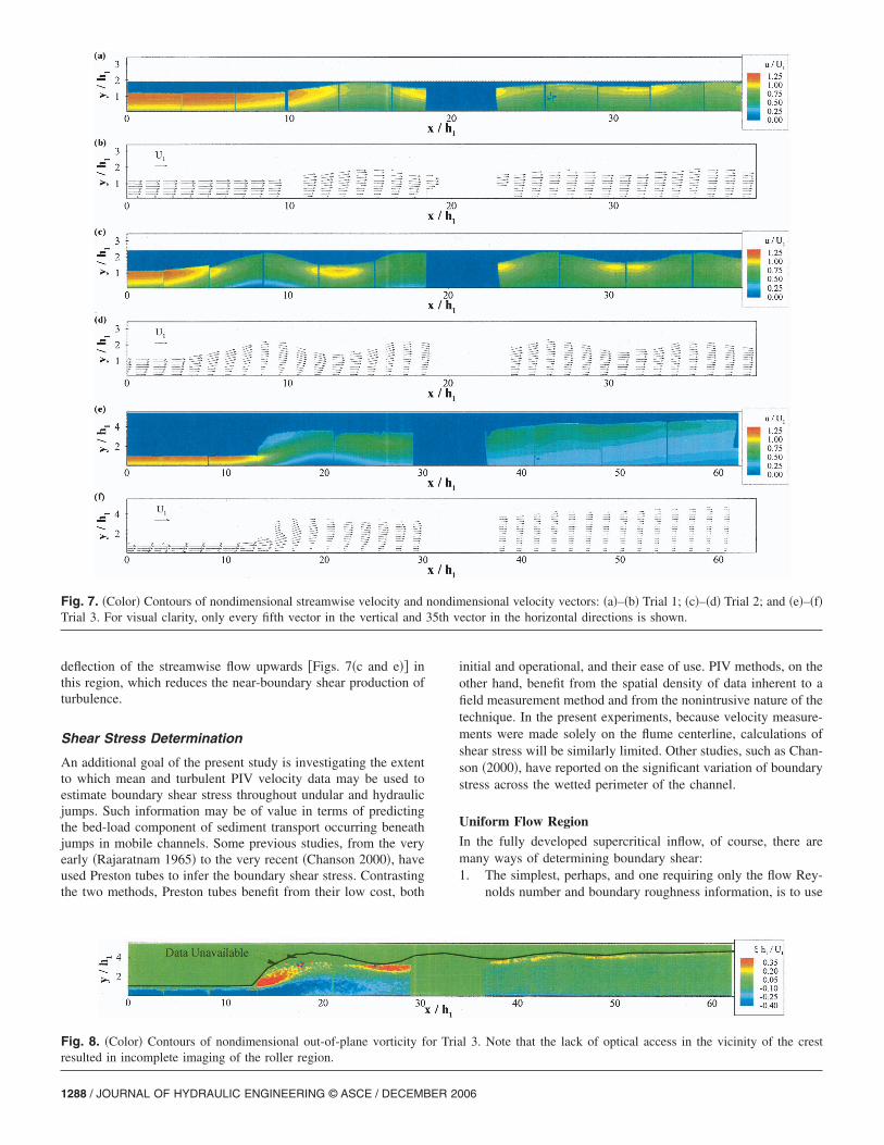
Ensemble averaged mean velocity data for the three trials arepresented in Fig. 7. For each case, a contour plot of the stream-wise velocity component and a two-dimensional velocity vectormap are presented. Note that velocities have been normalized byU1 and that distances have been normalized by h1. Second, for thesake of clarity in the vector maps, only every fifth vector in thevertical and every 35th vector in the horizontal is plotted. Thisamounts to only �0.6% of the available vectors being displayed.Third, the plots are all undistorted, so that the true aspect ratios ofthe jumps are preserved. Finally, recall that the origin in all caseswas taken to be the upstream edge of the upstream acrylic panelin the flume bottom.

The contour and vector plots all demonstrate a clear boundarylayer structure in the incoming supercritical flow. For the weakestjump studied, there is only a slight disruption to this boundarylayer profile throughout the extent of the jump. For the interme-diate jump, the subcritical flow is much more wavy in structure,with regions of high velocity in the troughs of the undular profile.The strongest jump studied is the one closest to a classicalhydraulic jump. The high velocity inflow deflects upwards under-neath the first crest, much like a wall-jet detaching from a bound-ary. The extremely low velocity underneath the roller regionsuggests a significant reduction in boundary shear in that area.

Out-of-plane vorticity is easily derived from the mean velocityfields. For the lowest two Froude numbers studied, where rollerswere absent, the only significant vorticity was the negative�clockwise� vorticity near the bottom boundary of the flume. Inthe strongest jump, however, and as illustrated in Fig. 8, positivevorticity was observed in the roller region and in the first troughof the undular flow downstream. For clarity, the free surface isalso plotted. As discussed previously, three-dimensional effectsand a high bubble fraction prevented full optical access to theroller region, hence the gap in the data in the roller and crestregions.

Turbulent Velocity Data

Similar contour plots of the turbulent velocity fields are readilycreated from the ensembles. As one example, consider horizontalvelocity fluctuations in the roller region from Trial 3, as shown inFig. 9. In this figure, only the region near the roller has beenshown. In the supercritical approach flow, the highest values ofurms� , which are on the order of 10% of the depth-averaged meanvelocity, are found near the bottom boundary, due to the boundaryshear. In the roller region itself, much higher values of urms� , onthe order of 40% of U1, are found in close proximity to the freesurface. These results are consistent with those of Misra et al.�2005� from their study of a slightly weaker jump.

The vertical distributions of both urms� and vrms� in the super-critical approach flow and directly underneath the first crest areshown in Fig. 10 for all three trials. For Trial 1, the mildest case,there is very little qualitative difference between the two longitu-dinal stations. Quantitatively, the turbulent velocities are slightlyhigher underneath the crest. Trials 2 and 3 display some similaritywith each other and significant differences with Trial 1. The pro-files of vrms� underneath the crests are now reversed, with highervalues nearer the free surface than the bottom. Additionally, theprofiles of urms� show two peaks, one near the free surface and theother near the bottom. Comparison of Figs. 10�b, d and f� revealsthat the near-bottom peak in urms� underneath the crest moves
steadily upwards with increasing F. This is a consequence of the

deflection of the streamwise flow upwards �Figs. 7�c and e�� inthis region, which reduces the near-boundary shear production ofturbulence.

Shear Stress Determination

An additional goal of the present study is investigating the extentto which mean and turbulent PIV velocity data may be used toestimate boundary shear stress throughout undular and hydraulicjumps. Such information may be of value in terms of predictingthe bed-load component of sediment transport occurring beneathjumps in mobile channels. Some previous studies, from the veryearly �Rajaratnam 1965� to the very recent �Chanson 2000�, haveused Preston tubes to infer the boundary shear stress. Contrastingthe two methods, Preston tubes benefit from their low cost, both

Fig. 7. �Color� Contours of nondimensional streamwise velocity andTrial 3. For visual clarity, only every fifth vector in the vertical and

Fig. 8. �Color� Contours of nondimensional out-of-plane vorticity fresulted in incomplete imaging of the roller region.


initial and operational, and their ease of use. PIV methods, on theother hand, benefit from the spatial density of data inherent to afield measurement method and from the nonintrusive nature of thetechnique. In the present experiments, because velocity measure-ments were made solely on the flume centerline, calculations ofshear stress will be similarly limited. Other studies, such as Chan-son �2000�, have reported on the significant variation of boundarystress across the wetted perimeter of the channel.

Uniform Flow RegionIn the fully developed supercritical inflow, of course, there aremany ways of determining boundary shear:1. The simplest, perhaps, and one requiring only the flow Rey-

nolds number and boundary roughness information, is to use

ensional velocity vectors: �a�–�b� Trial 1; �c�–�d� Trial 2; and �e�–�f�ector in the horizontal directions is shown.

l 3. Note that the lack of optical access in the vicinity of the crest

nondim35th v

or Tria

06

a friction factor approach. Application of the Colebrook-White equation

1

f1/2 = − 2.0 log� �/Dh

3.7+

2.51

RDhf1/2�

where ��roughness height, allows for the determination ofthe friction factor f and hence the boundary shear �0. Onelimitation of this approach is that it necessarily assumes thatthe shear is uniform over the wetted perimeter. Given theacrylic walls and bottom of the flume, ��0 was assumed forthe calculations.

2. Second-order velocity statistics can also be used to estimateshear stress. For the case of uniform flow, Nezu and Rodi�1986� provide the following well-known empirical relationsdescribing the vertical variation of the horizontal and verticalroot mean square �rms� velocity fluctuations

urms�

u* = Duexp�− �u

y

h� �1�

vrms�

u* = Dvexp�− �vy

h� �2�

where h�flow depth; and u*=��0 /��shear velocity. Theconstants �u and �v have been shown to equal 1.0 and 0.67and the constants Du and Dv have been shown to equal 2.30and 1.27. Slight deviations from these universal relations areexpected in the viscous layer near the boundary and close tothe free surface. For the present measurements, it is straight-forward to fit these curves to the data �Figs. 10�a, c and e��,treating the shear velocity as a fitting parameter, in the su-percritical approach flow.

3. Finally, knowledge of the Reynolds stresses can be used todeduce shear at the boundary as well. From boundary layerequations, it is straightforward to show that, for uniformflow, the vertical variation of total stress is linear. Over mostof the flow depth, the total stress is dominated by the Rey-nolds stress, due to the weak mean velocity gradients awayfrom the boundary. A linear fit to the Reynolds stress in thisouter region can be extrapolated to the boundary in order todetermine �0. For the present experiments, this is demon-strated in Fig. 11. As shown, the vertical variation of theReynolds stress in the outer region is indeed linear for thesupercritical approach flows of all three trials. Also shown

Fig. 9. �Color� Contours of nondimensional values of urms� for Trial 3.ratio has not been preserved as in the previous figures.

are the vertical profiles underneath the first crests of the three

JOURNAL

jumps. For Trials 2 and 3, the Reynolds stress becomes nega-tive away from the boundary, indicating the reversal in meanvelocity shear seen near the surface. It is clear that, outside ofthe uniform approach flow, use of boundary layer theory indeducing boundary shear from turbulent stresses is notpossible.

A summary of the boundary shear stresses in the approachflows, obtained via these three methods, is provided in Table 2.For Trials 2 and 3, the results are fairly consistent, with coeffi-cients of variation of 10 and 14%, respectively. For Trial 1, it isclear that the results from the velocity fluctuations are at oddswith the other two methods. While it is possible that this is aReynolds number or Froude number effect, adequate data on thevariation of the coefficients in Eqs. �1� and �2� with R and F donot exist.

Nonuniform Flow RegionOf greater interest is the assessment of the extent to which PIVdata may be used to deduce boundary shear in regions of nonuni-form flow. Here, two candidate methods exist: the use of well-known vertical distributions of mean velocity in wall-boundedshear flows and the direct computation of shear from velocity datawithin the viscous sublayer:1. Regarding the first method, the application of boundary layer

theory to jumps was used by Streinruck et al. �2003� in theirtheoretical study of turbulent undular jumps. While the loga-rithmic overlap equation �White 1991� is a popular choice,care must be taken to apply it only in its range of applicabil-ity, approximately 30y+300, where y+=yu* /� representswall units. Montes and Chanson �1998� state that Coles’ lawof the wake is a superior choice, given that it may be appliedthroughout the full depth of the flow. Coles’ law is given by

u

u* =1

loge�y+� + B +

2�

f�� 3�

In this equation, u�streamwise velocity; and andB�near-universal constants, taken to be 0.4 and 5.0, respec-tively. For rough-wall flows, the second parameter can varyconsiderably.

The wake parameter � depends upon the pressure gradi-ent in the flow and can be treated as a free parameter. The

xes have been zoomed in to focus on the roller region, and the aspect
The a
wake function f�� is given by


Fig. 10. Vertical profiles of horizontal and vertical turbulent velocities: �a� Trial 1, approach flow; �b� Trial 1, underneath first crest; �c� Trial 2,approach flow; �d� Trial 2, underneath first crest; �e� Trial 3, approach flow; and �f� Trial 3, underneath first crest


f�� = 3�2 − 2�3, � =y

�4�

where �boundary layer thickness. In the fully developedsupercritical approach flow, the boundary layer thickness isequal to the flow depth, while in the jump itself, the defini-

Fig. 11. Vertical profiles of Reynolds stress −�u�v�: �a� Trial 1, apprTrial 2, underneath first crest; �e� Trial 3, approach flow; and �f� Tria

tion of is much less clear. As discussed by White �1991�,

JOURNAL

ambiguity in the definition of can lead to a poor agreementbetween Coles’ law and experimental data for nonequilib-rium flows. Therefore, the present analysis will fit Coles’ lawto the data, treating u*, �, and all as free parameters.

This least-squares analysis was done using Matlab’s fmin-

ow; �b� Trial 1, underneath first crest; �c� Trial 2, approach flow; �d�derneath first crest

oach fll 3, un

con function, which finds the constrained minimum of a


function of multiple variables. As an example, Fig. 12 showsexperimental data and Coles’ law for several different veloc-ity profiles. For each of the three trials, velocity profiles inthe supercritical approach flow and directly underneath thefirst crest are considered. In all cases, even beneath thecrests, the agreement between the data and the curve fit isextremely good. This suggests that vertical mean velocityprofiles throughout the jumps can be used to estimate theboundary shear. The corresponding boundary shear valuesare summarized in Table 3. Note that the values in the ap-proach flow are in good agreement with those obtained byother methods and that the values beneath the crests are dra-matically reduced.

To support the validity of using Coles’ law in the presentexperiments, note first of all that no flow reversal was ob-served near the boundary. Beneath the crest in Trial 3, thestreamwise velocity near the boundary was indeed extremelysmall, but still positive. Next, Coles �1956� investigates theapplication of the wake law to the adverse-pressure gradientdata of Schubauer and Klebanoff �1950� and others and isable to show excellent agreement between the data and Eq.�3�. To do so, Coles �1956� allows u*, , and � to all besmoothly varying functions of streamwise distance x, theprecise strategy adopted by the present writers.

2. Turning now to the second method, it is possible to obtainthe shear stress directly from velocity measurements withinthe viscous sublayer. In this constant stress region, generallydefined as y+5, the total stress is dominated by the laminarstress, calculated from

�xy = ��u

�y�5�

where ��dynamic viscosity. In principle, PIV can easilymake measurements in the sublayer. In practice, however, theconstraint of needing a grid point within the viscous sublayerrequires a very high magnification; i.e., the camera must bezoomed in on a very small region close to the boundary. Inthe present experiments, the camera was kept fairly zoomedout in order to �1� capture the full depth of the flow; and �2�cover a large streamwise extent ��1 m� with a minimalnumber of camera positions. As a result, the sublayer wasresolved only in the low-stress region underneath the firstcrest of the jumps.

To illustrate this, recall the typical grid spacings discussedearlier. The first grid point above the flume bottom was typi-cally at a height of about 0.75 mm. With a shear velocity of4 cm s−1, which was typical of the approach flows, the sub-layer thickness is approximately 0.1 mm, which is far lessthan the grid resolution. Underneath the crests, where theshear is very low �u*�0.5 cm s−1�, the sublayer thickness is

Table 2. Boundary Shear Stress, in Supercritical Approach Flow Region,as Derived from Colebrook-White Equation, Vertical Distribution ofTurbulent Velocities, and Vertical Distribution of Reynolds Stress

Trial 1 2 3

Colebrook-White �Pa� 1.37 1.88 3.96

urms� �Pa� 2.40 1.65 3.85

vrms� �Pa� 3.29 1.85 2.96

Reynolds stress �Pa� 1.21 1.50 3.08

on the order of 1 mm. In these low stress regions, therefore,


Fig. 12. Vertical mean velocity profiles in the supercritical approachflow and underneath the first crest. For clarity, only every other datapoint is shown. Also shown are the curve fits obtained with Cole’slaw: �a� Trial 1; �b� Trial 2; and �c� Trial 3.

06

the PIV measurements of mean velocity should lead directlyto the boundary stress.

Streamwise distributions of shear stress from the two methodsare compared in Fig. 13 for all three trials. Also shown are thestreamwise distributions of the elevation of the first grid point inwall units. Consider first the results obtained from the applicationof Coles’ law and note that, in order to maximize the visual claritynear the origin of the vertical axis, the axis upper limits truncatethe results in the supercritical approach flows. Next, note that theshear stress is inversely proportional to flow depth, with maxi-mum values in the supercritical approach flows and minimumvalues beneath the crests of the jumps. In Trials 1 and 2, whichare undular in nature, the shear rises as the flow acceleratesthrough the trough following each crest. In Trials 2 and 3, thereduction in shear below the crest is particularly strong, with theobserved shear nearly vanishing �recall Table 3�.

When the results from the two methods are compared, Fig. 13indicates a significant discrepancy over much of the extent of the

Table 3. Boundary Shear Stress, in Supercritical Approach Flow andBeneath First Crest, Derived from Application of Coles’ Law to MeanVertical Velocity Profile

TrialApproach �0

�Pa�Crest �0

�Pa�

1 1.31 0.300

2 1.59 0.030

3 3.81 0.031

Fig. 13. Streamwise profiles of dimensional boundary shear stress, asprofiles determined from Cole’s law. Finally, the streamwise distribut1; �b� Trial 2; and �c� Trial 3.

JOURNAL

jumps. From the preceding discussion, it is clear that this is due tothe fact that the first available grid point from the PIV analysisgenerally lies outside of the viscous sublayer. As a result, shearstress derived from Eq. �5� and an assumed linear velocity profilewill underestimate the shear, as the figure confirms. In low-shearregions, where the vertical position of the first grid point ap-proaches �10 wall units, however, the agreement between thetwo stress estimates is quite good. For the present experiments,these regions are limited to the first crests of the jumps. A highermagnification factor, through the use of a higher resolution cam-era or a smaller imaged area, will extend the range within whichthe stress can reliably be estimated with Eq. �5�.

As a final point, the present shear stress results can be com-pared with those obtained by Chanson �2000� with a Preston tube.In particular, he presents data on the streamwise variation of cen-terline shear stress for a run with F1=1.48, which is in proximityto Trial 1 of the present study. His measurements show that theshear stress underneath the first crest is 22% that of the supercriti-cal approach flow. The present measurements, from Coles’ law�Fig. 13�a�� show a value of 20%, which is in good agreement.

Concluding Remarks

PIV measurements of free undular and hydraulic jumps have beenperformed. For three different Froude numbers, ensembles of 400image pairs at 10 different streamwise locations were tiled to-gether into “mosaic” images of the jumps. Qualitatively, plots of

ined from Newton’s law of viscosity. Also shown are the shear stressthe elevation of the first grid point in wall units are shown: �a� Trial

determions of


mean variables such as velocity and vorticity yielded a highlyresolved look at the kinematics inside these transitional flows.Only for the highest Froude number was a vortical roller detected.

Several methods for quantitatively determining the boundaryshear stress from the PIV measurements were investigated. Ofthese, two proved capable of determining the boundary shear inregions other than the uniform supercritical approach flow. Coles’law of the wake was applied to vertical velocity profiles at allstreamwise locations, yielding the distribution of boundary shearwith streamwise distance. The boundary layer thickness, the shearvelocity, and the wake parameter were all treated as smoothlyvarying functions of streamwise distance and were determinedthrough constrained optimization.

The boundary stress was also determined directly from thefluid strain rate in the viscous sublayer. The success of thismethod relies upon the ability of the PIV measurements to resolvethe sublayer. For the present experiments, this was possible onlyin the low-stress regions underneath the crests. By increasing themagnification and imaging a smaller field of view, PIV measure-ments will be able to determine the boundary stress at all stream-wise locations using this approach.

The technical challenges associated with applying PIV to evenstronger hydraulic jumps are significant. A high void fraction, dueto the aeration at the roller, will obscure the optical path betweenthe object and image planes. This will lead to blurry images andpoor image correlations. If the emphasis is solely on boundaryshear, high magnification imaging of the near-boundary regiononly will help to alleviate this difficulty, as the bubbles resideprimarily in the upper regions of the flow.

Notation

The following symbols are used in this paper:B � logarithmic velocity profile constant;b � flume width;

Dh � hydraulic diameter;�Du ,Dv ,�u ,�v�

� coefficients;F1 � supercritical Froude number;

f � friction factor;h � general flow depth;

h1 � supercritical flow depth;R � Reynolds number;

U1 � depth-averaged supercritical flow velocity;�u ,v� � streamwise and vertical velocity components;

�u� ,v�� horizontal and vertical velocity fluctuations;u* � shear velocity;

�x ,y� � horizontal and vertical position; � boundary layer thickness;� � roughness height;� � scaled boundary layer coordinate; � von Kármán constant;� � kinematic viscosity;� � vorticity;� � shear stress;

� � Cole’s law wake parameter; and
�0 � boundary shear stress.

References

Chanson, H. �2000�. “Boundary shear stress measurements in undularflows: Application to standing wave bed forms.” Water Resour. Res.,36�10�, 3063–3076.

Chanson, H., and Brattberg, T., �2000�. “Experimental study of the air-water shear flow in a hydraulic jump.” Int. J. Multiphase Flow, 26,583–607.

Chanson, H., and Montes, J., �1995�. “Characteristics of undular hydrau-lic jumps: Experimental apparatus and flow patterns.” J. Hydraul.Eng. 121�2�, 129–144.

Chistensen, K., Soloff, S., and Adrian, R., �2000�. “PIV Sleuth—Integrated acquisition, interrogation, and validation software for par-ticle image velocimetry.” Rep. No. 943, Dept. of Theoretical and Ap-plied Mechanics, University of Illinois, Champaign, Ill.

Coles, D. �1956� “The law of the wake in the turbulent boundary layer.”J. Fluid Mech., 1, 191–226.

Hornung, H., Willert, C., and Turner, S. �1995�. “The flow field down-stream of a hydraulic jump.” J. Fluid Mech., 287, 299–316.

Kirkgoz, M., and Ardichoglu, M. �1997�. “Velocity profiles of developingand developed open channel flow.” J. Hydraul. Eng., 123�12�, 1099–1105.

Leutheusser, H., and Kartha, V. �1972�. “Effects of inflow condition onhydraulic jumps.” J. Hydr. Div., 98�8�, 1367–1385.

Liu, M., Rajaratnam, N., and Zhu, D. �2004�. “Turbulence structure ofhydraulic jumps of low Froude numbers.” J. Hydraul. Eng., 130�6�,511–520.

Long, D., Steffler, P., and Rajaratnam, N. �1990�. “Lda study of flowstructure in submerged hydraulic jump.” J. Hydraul. Res., 28�4�,437–460.

Misra, S., Kirby, J., Brocchini, M., Veron, F., Thomas, M., and Kamb-hamettu, C. �2005�. “Hydraulic jump as a quasi-steady spillingbreaker: An experimental study of similitude.” J. Fluid Mech., inpress.

Montes, J., and Chanson, H. �1998�. “Characteristics of undular hydraulicjumps: Experiments and analysis.” J. Hydraul. Eng., 124�2�, 192–205.

Murzyn, F., Mouaze, D., and Chaplin, J. �2005�. “Optical fibre probemeasurements of bubbly flow in hydraulic jumps.” Int. J. MultiphaseFlow, 31, 141–154.

Nezu, I., and Rodi, W. �1986�. “Open-channel flow measurements with alaser Doppler anemometer.” J. Hydraul. Eng., 1125�5�, 335–355.

Ohtsu, I., Yasuda, Y., and Gotoh, H. �2001�. “Hydraulic condition forundular-jump formations.” J. Hydraul. Res., 39�2�, 203–209.

Ohtsu, I., Yasuda, Y., and Gotoh, H. �2003�. “Flow conditions of undularhydraulic jumps in horizontal rectangular channels.” J. Hydraul. Eng.,129�12�, 948–955.

Raffel, M., Willet, C., and Kompenhans, J. �1998�. Particle image veloci-metry, Springer, Berlin.

Rajaratnam, N. �1965�. “The hydraulic jump as well jet.” J. Hydr. Div.,91�5�, 107–134.

Resch, F., Leutheusser, H., and Alemum, S. �1974�. “Bubbly two-phaseflow in hydraulic jump.” J. Hydr. Div., 100�1�, 137–149.

Rouse, H., Siao, T. T., and Nagaratnam, S. �1958�. “Turbulence charac-teristics of the hydraulic jump.” J. Hydr. Div., 84�1�, 1–30.

Schubauer, G., and Klebanoff, P. �1950�. “Investigation of separation ofthe turbulent boundary layer.” Rep. No. 2133, National AdvisoryCommittee for Aeronautics, Washington, D.C.

Streinruck, H., Schneider, W., and Grillhofer, W. �2003�. “A multiplescales analysis of the undular hydraulic jump in turbulent open chan-nel flow.” Fluid Dyn. Res., 33, 41–55.

Svendsen, I., Veeramony, J., Bakunin, J., and Kirby, J. �2000�. “The flowin weak turbulent hydraulic jumps.” J. Fluid Mech., 418, 25–57.

White, F. �1991�. Viscous fluid flow, 2nd Ed., McGraw-Hill, New York.

06

Particle Image Velocity Measurements of Undular and ... · Particle Image Velocity Measurements of...

Documents

Transcript of Particle Image Velocity Measurements of Undular and ... · Particle Image Velocity Measurements of...