Partial Least Squares For Researchers: An overview and ... · Stressful Change Events
50
opyright 2002 by Wynne W. Chin. Copyright 2002 by Wynne W. Chin. All rights reserved. Slide 1 Partial Least Squares For Researchers: An overview and presentation of recent advances using the PLS approach Wynne W. Chin C.T. Bauer College of Business University of Houston Copyright 2002 by Wynne W. Chin. All rights reserved. Slide 2 Some questions • I would like a description of how to interpret the models. • What do all of Greek letters mean? • Which fit statistics are most important? • What are the rules of thumb for the fit statistics? • What are paths and how are the path statistics interpreted?
Transcript of Partial Least Squares For Researchers: An overview and ... · Stressful Change Events
1Copyright 2002 by Wynne W. Chin.
All rights reserved
Copyright 2002 by Wynne W. Chin. All rights reserved. Slide 1
Partial Least Squares ForResearchers: An overviewand presentation of recentadvances using the PLS
approachWynne W. Chin
C.T. Bauer College of BusinessUniversity of Houston
Copyright 2002 by Wynne W. Chin. All rights reserved. Slide 2
Some questions
• I would like a description of how tointerpret the models.
• What do all of Greek letters mean?• Which fit statistics are most important?• What are the rules of thumb for the fit
statistics?• What are paths and how are the path
statistics interpreted?

2Copyright 2002 by Wynne W. Chin.
All rights reserved
Copyright 2002 by Wynne W. Chin. All rights reserved. Slide 3
Some questions
• What are the advantages/disadvantages of usingthe measurement models (PLS or SEM) ascompared to using factor analysis (exploratory andconfirmatory) and item reliability analysis?
• Is it possible to use the measurement models tounderstand construct validity (discriminantvalidity and convergent validity)?
Copyright 2002 by Wynne W. Chin. All rights reserved. Slide 4
Some questions
• How much impact does sample size have? Iam aware of the 7-10 observations per itemrule of thumb, but how sensitive are thestatistics to variations in this rule of thumb?(i.e., as a reviewer, when should I questionsthe use of one of the techniques?)
• When to use PLS v. LISREL etc. What arethe advantages of PLS?
3Copyright 2002 by Wynne W. Chin.
All rights reserved
Copyright 2002 by Wynne W. Chin. All rights reserved. Slide 5
Some questions
• How to interpret results - I'm a little more familiarwith LISREL, but with many of these approachesthere are multiple indicators of the quality of thesolution (i.e., fit indices in LISREL, etc.) whichmakes it difficult to know which ones toreport? Also, when do I have a "good" solution?
• What do I look for when I am reviewing a paperthat uses these techniques? What things should bereported, how might I evaluate what is reported.
Copyright 2002 by Wynne W. Chin. All rights reserved. Slide 6
Agenda1. List conditions that may suggest using PLS.
2. See where PLS stands in relation to other multivariate techniques.
3. Demonstrate the PLS-Graph software package for interactive PLS analyses.
4. Gain some understanding of causal diagrams and go over the LISRELapproach.
5. Go over the PLS algorithm - implications for sample size, data distributions& epistemological relationships between measures and concepts.
6. Cover notions of formative and reflective measures.
7. See how PLS and LISREL compare and compliment one another.
8. Cover statistical re-sampling techniques for significance testing.
9. Look at second order factors, interaction effects, and multi-groupcomparisons.
10. Recap of the issues and conditions for using PLS.
4Copyright 2002 by Wynne W. Chin.
All rights reserved
Copyright 2002 by Wynne W. Chin. All rights reserved. Slide 7
Do any of the following pertainto you?
• Do you work with theoretical models thatinvolve latent constructs?
• Do you have multicollinearity problemswith variables that tap into the same issues?
• Do you want to account for measurementerror?
• Do you have non-normal data?
Copyright 2002 by Wynne W. Chin. All rights reserved. Slide 8
Do any of the following pertainto you? (continued)
• Do you have a small sample set?• Do you wish to determine whether the
measures you developed are valid andreliable within the context of the theory youare working in?
• Do you have formative as well as reflectivemeasures?

5Copyright 2002 by Wynne W. Chin.
All rights reserved
Copyright 2002 by Wynne W. Chin. All rights reserved. Slide 9
Being a component approach,PLS covers:
• principal component,• canonical correlation,• redundancy,• inter-battery factor,• multi-set canonical correlation, and• correspondence analysis as special cases
Copyright 2002 by Wynne W. Chin. All rights reserved. Slide 10
PLS
RedundancyAnalysis
ESSCA CanonicalCorrelation
MultipleRegression
MultipleDiscriminant
Analysis
Analysis ofVariance
Analysis ofCovariance
PrincipalComponents
SimultaneousEquations
FactorAnalysis
CovarianceBased SEM
A B means B is a special case of A

6Copyright 2002 by Wynne W. Chin.
All rights reserved
Copyright 2002 by Wynne W. Chin. All rights reserved. Slide 11
ConfirmatoryLatent
StructureAnalysis
Latent ClassAnalysis
LatentProfile
Analysis
GuttmanPerfectScale Analysis
ConfirmatoryMultidimensional
Scaling
MultidimensionalScaling
A B means B is a special case of A
Copyright 2002 by Wynne W. Chin. All rights reserved. Slide 12
Background of the PLS-Graphmethodology
• Statistical basis initially formed in the late60s through the 70s by econometricians inEurope.
• A Fortran based mainframe softwarecreated in the early 80s. PC version in mid80s.
• Has been used by companies such as IBM,Ford, ATT and GM.

7Copyright 2002 by Wynne W. Chin.
All rights reserved
Copyright 2002 by Wynne W. Chin. All rights reserved. Slide 13
Background of the PLS-Graphmethodology (continued)
• The PLS-Graph software has been underdevelopment for the past 9 years. Academic beta testers include QueensUniversity, Western Ontario, UBC,MIT,UCF, AGSM, U of Michigan, U ofIllinois, Florida State, National Universityof Singapore, NTU, Ohio State, Wharton,UCLA, Georgia State, the University ofHouston, and City U of Hong Kong.
Copyright 2002 by Wynne W. Chin. All rights reserved. Slide 14“But we just don’t have the technology to carry it out.”

8Copyright 2002 by Wynne W. Chin.
All rights reserved
Copyright 2002 by Wynne W. Chin. All rights reserved. Slide 15
Let’s See How It Works
Copyright 2002 by Wynne W. Chin. All rights reserved. Slide 16
Constructs Source Original DefinitionPerceived Usefulness Davis (1989) The degree to which a person believes
that using a particular system wouldenhance his or her job performance.
Perceived Ease of Use Davis (1989) The degree to which a person believesthat using a particular system would befree of effort.
Compatibility Moore andBenbasat (1991)
The degree to which an innovation isperceived as being consistent with theexisting values, needs, and pastexperiences of potential adopters.
Voluntariness Moore andBenbasat (1991)
The degree to which use of the innovationis perceived as being voluntary, or of freewill.
ResultDemonstrability
Moore andBenbasat (1991)
The degree to which the results of aninnovation are communicable to others.
Adoption intention authors A measure of the strength of one'sintention to perform a behavior (e.g., usevoice mail).

9Copyright 2002 by Wynne W. Chin.
All rights reserved
Copyright 2002 by Wynne W. Chin. All rights reserved. Slide 17
Copyright 2002 by Wynne W. Chin. All rights reserved. Slide 18
INTENTION
VINT1 I presently intend to use Voice Mailregularly:
VINT2 My actual intention to use Voice Mailregularly is:
VINT3 Once again, to what extent do you at presentintend to use Voice Mail regularly:

10Copyright 2002 by Wynne W. Chin.
All rights reserved
Copyright 2002 by Wynne W. Chin. All rights reserved. Slide 19
VOLUNTARINESS
VVLT1 My superiors expect (would expect) me touse Voice Mail.
VVLT2 My use of Voice Mail is (would be)voluntary (as opposed to required by mysuperiors or job description).
VVLT3 My boss does not require (would notrequire) me to use Voice Mail.
VVLT4 Although it might be helpful, using VoiceMail is certainly not (would not be)compulsory in my job.
Copyright 2002 by Wynne W. Chin. All rights reserved. Slide 20
COMPATIBILITY
VCPT1 Using Voice Mail is (would be) compatible with all aspectsof my work.
VCPT2 Using Voice Mail is (would be) completely compatiblewith my current situation.
VCPT3 I think that using Voice Mail fits (would fit) well with theway I like to work.
VCPT4 Using Voice Mail fits (would fit) into my work style.

11Copyright 2002 by Wynne W. Chin.
All rights reserved
Copyright 2002 by Wynne W. Chin. All rights reserved. Slide 21
PERCEIVED USEFULNESS
VRA1 Using Voice Mail in my job enables (wouldenable) me to accomplish tasks more quickly.
VRA2 Using Voice Mail improves (would imporve)my job performance.
EASE OF USE
VEOU1 Learning to operate Voice Mail is (would be)easy for me.
VEOU2 I find (would find) it easy to get Voice Mailto do what I want it to do.
Copyright 2002 by Wynne W. Chin. All rights reserved. Slide 22
RESULT DEMONSTRABILITY
VRD1 I would have no difficulty telling othersabout the results of using Voice Mail.
VRD2 I believe I could communicate to others theconsequences of using Voice Mail.
VRD3 The results of using Voice Mail are apparentto me.
VRD4 I would have difficulty explaining whyusing Voice Mail may or may not bebeneficial.

12Copyright 2002 by Wynne W. Chin.
All rights reserved
Copyright 2002 by Wynne W. Chin. All rights reserved. Slide 23
ATTITUDE
All things considered, my using Voice Mail is (would be):
pleasant unpleasant
good bad
likable dislikable
harmful beneficial
wise foolish
negative positive
valuable worthless
Copyright 2002 by Wynne W. Chin. All rights reserved. Slide 24

13Copyright 2002 by Wynne W. Chin.
All rights reserved
Copyright 2002 by Wynne W. Chin. All rights reserved. Slide 25
ΑΒΓΛΕΖΗΘΙΚΛΜΝΞΟΠΡΣΤΥΦΧΨΩ
αβγδε
ζηθικλµν
ξοπρ
στυϕχψω
alphabetagammadeltaepsilonzetaetathetaiotakappalambdamunuxiomicronpirhosigmatauupsilonphichipsiomega
Do we need Greek letters?
Copyright 2002 by Wynne W. Chin. All rights reserved. Slide 26
Introduction To StructuralEquation Modeling
Structural Equation Modeling (SEM) represents an approachwhich integrates various portions of the research process in anholistic fashion. It involves:
•development of a theoretical frame where each concept draw itsmeaning partly through the nomological network of concepts it isembedded,
•specification of the auxillary theory which relates empirical measuresand methods for measurement to theoretical concepts
•constant interplay between theory and data based on interpretat ion ofdata via ones objectives, epistemic view of data to theory, dataproperties, and level of theoretical knowledge and measurement.

14Copyright 2002 by Wynne W. Chin.
All rights reserved
Copyright 2002 by Wynne W. Chin. All rights reserved. Slide 27
SEM as theoretical empiricismLay Person Narrative
Scientific Narrative
Conceptual Representation
Mathematical Representation
Empirical World
Aggregated Data
Data - measurements from asampled representation
Theory Empiricism
Copyright 2002 by Wynne W. Chin. All rights reserved. Slide 28
Statistically - SEM represents a secondgeneration analytical technique which:
• Combines an econometric perspectivefocusing on prediction and
• a psychometric perspective modeling latent(unobserved) variables inferred fromobserved - measured variables.
• Resulting in greater flexibility in modelingtheory with data compared to firstgeneration techniques

15Copyright 2002 by Wynne W. Chin.
All rights reserved
Copyright 2002 by Wynne W. Chin. All rights reserved. Slide 29
SEM modeling flexibilityinclude:
• Modeling multiple predictors and criterionvariables
• Construct latent (unobservable) variables• Model errors in measurement for observed
variables due to noise and other unique factors• Confirmatory analysis - Statistically test prior
substantive/theoretical and measurementassumption against empirical data
Copyright 2002 by Wynne W. Chin. All rights reserved. Slide 30
Viewed as an extension or generalization offirst generation techniques - SEM can beused to perform the following analyses :
• Factor or component based analysis
• Discriminant analysis
• Multiple regression
• Canonical correlation
• MANOVA

16Copyright 2002 by Wynne W. Chin.
All rights reserved
Copyright 2002 by Wynne W. Chin. All rights reserved. Slide 31
• Provide a non-technical introduction to the logicbehind structural equation modeling (SEM) -both covariance and partial least squares based
• Introduce the casual diagramming approach andconcepts underlying it
• Contrast SEM to other methods (in particularmultiple regression) and demonstrate whyaccounting for measurement error using SEM isvery important
At this point, I’d like to:
Copyright 2002 by Wynne W. Chin. All rights reserved. Slide 32
F1F2 F3 F4
Y4 Y5F4
Y1 Y Y32
e1 e2
e3 e5e4

17Copyright 2002 by Wynne W. Chin.
All rights reserved
Copyright 2002 by Wynne W. Chin. All rights reserved. Slide 33
X1
F1
e1 e2
Copyright 2002 by Wynne W. Chin. All rights reserved. Slide 34
F1 F2 F3 F4
Y4 Y5F4
Y1 Y Y32
e1 e 2
e 3 e 5e 4
Postivistic MechanisticChoo Choo Train Model
X1
F 1
e 1 e2
Holistic, gwounded (as inliving-in-the-hole-in-the-gwound), "wabbit" model
18Copyright 2002 by Wynne W. Chin.
All rights reserved
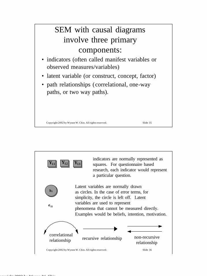
Copyright 2002 by Wynne W. Chin. All rights reserved. Slide 35
• indicators (often called manifest variables orobserved measures/variables)
• latent variable (or construct, concept, factor)• path relationships (correlational, one-way
paths, or two way paths).
SEM with causal diagramsinvolve three primary
components:
Copyright 2002 by Wynne W. Chin. All rights reserved. Slide 36
Y11 Y12 Y13indicators are normally represented assquares. For questionnaire basedresearch, each indicator would representa particular question.
η1
Latent variables are normally drawnas circles. In the case of error terms, forsimplicity, the circle is left off. Latentvariables are used to representphenomena that cannot be measured directly.Examples would be beliefs, intention, motivation.
ε11
correlationalrelationship recursive relationship non-recursive
relationship
19Copyright 2002 by Wynne W. Chin.
All rights reserved
Copyright 2002 by Wynne W. Chin. All rights reserved. Slide 37
ρ
1.0 1.0
η1
X1
η2
X2
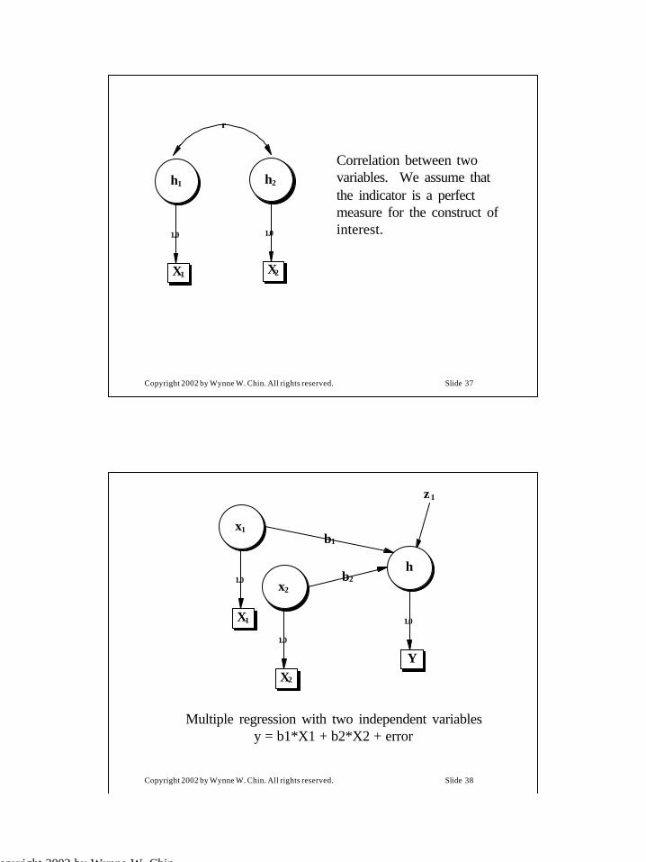
Correlation between twovariables. We assume thatthe indicator is a perfectmeasure for the construct ofinterest.
Copyright 2002 by Wynne W. Chin. All rights reserved. Slide 38
1.0
1.0
1.0
β1
β2
ξ1
X1
ξ2
X2
η
Y
ζ1
Multiple regression with two independent variablesy = b1*X1 + b2*X2 + error

20Copyright 2002 by Wynne W. Chin.
All rights reserved
Copyright 2002 by Wynne W. Chin. All rights reserved. Slide 39
Simple Regression
Multiple RegressionPath Analysis
Causal Chain System(Recursive)
Copyright 2002 by Wynne W. Chin. All rights reserved. Slide 40
Path AnalysisInterdependent System
(Non-recursive)
21Copyright 2002 by Wynne W. Chin.
All rights reserved
Copyright 2002 by Wynne W. Chin. All rights reserved. Slide 41
dummy0,1
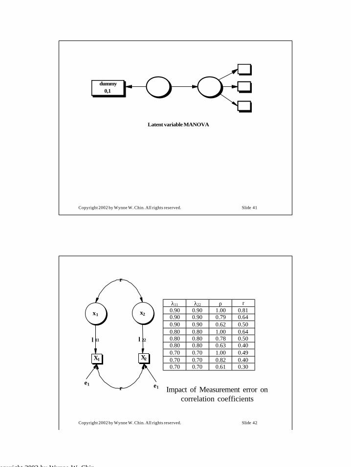
Latent variable MANOVA
Copyright 2002 by Wynne W. Chin. All rights reserved. Slide 42
ε
λ11
ρ
λ22
r
ξ1
X1
ξ2
X2
ε11
λ11 λ22 ρ r0.90 0.90 1.00 0.810.90 0.90 0.79 0.640.90 0.90 0.62 0.500.80 0.80 1.00 0.640.80 0.80 0.78 0.500.80 0.80 0.63 0.400.70 0.70 1.00 0.490.70 0.70 0.82 0.400.70 0.70 0.61 0.30
Impact of Measurement error oncorrelation coefficients
22Copyright 2002 by Wynne W. Chin.
All rights reserved
Copyright 2002 by Wynne W. Chin. All rights reserved. Slide 43
ρ
λ11λ12 λ13 λ21 λ23λ22
ξ1 ξ2
X11
ε11
X12
ε12
X13
ε13
X21
ε21
X22
ε22
Y2X
ε23
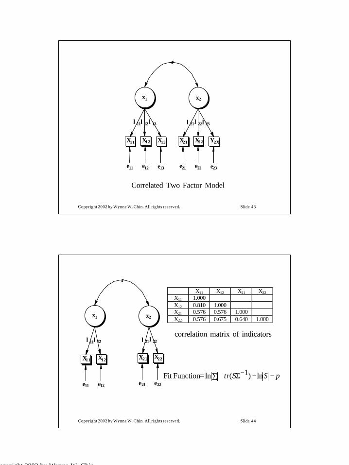
Correlated Two Factor Model
Copyright 2002 by Wynne W. Chin. All rights reserved. Slide 44
ρ
λ11λ12 λ21λ22
ξ1 ξ2
X11
ε11
X12
ε12
X21
ε21
X22
ε22
X11 X12 X21 X22X11 1.000X12 0.810 1.000X21 0.576 0.576 1.000X22 0.576 0.675 0.640 1.000
correlation matrix of indicators
pSStr −−−Σ+∑= ln)1(lnFunctionFit

23Copyright 2002 by Wynne W. Chin.
All rights reserved
Copyright 2002 by Wynne W. Chin. All rights reserved. Slide 45
More Graphical Representations
β23
γ 34
λ11λ12λ 13
λ21λ22λ23
λ31 λ 32λ 33 λ 41λ 42
λ 43β13
β 24
η1
η2
ζ2
η 3
ζ3
η 4
ζ4
Y11
ε11
Y12
ε12
Y13
ε13
Y21
ε 21
Y22
ε 22
Y23
ε 23
Y31
ε 31
Y32
ε 32
Y33
ε 33
Y41
ε 41
Y42
ε 42
Y43
ε 43
Copyright 2002 by Wynne W. Chin. All rights reserved. Slide 46
p1
p4
l4 l5 l6
l1 l2 l3
l7 l8 l9 l10 l11l12
p2
p3
F1
F2
F3
d1
F4
d2
x4
e 4
x 5
e 5
x6
e 6
x 1
e1
x2
e2
x 3
e3
y1
e7
y2
e8
y 3
e9
y 4
e10
y5
e11
y 6
e12
More Graphical Representations

24Copyright 2002 by Wynne W. Chin.
All rights reserved
Copyright 2002 by Wynne W. Chin. All rights reserved. Slide 47
p1
p4
l1 l2 l3
l7 l8l9 l10 l11
l12
p3
l4 l5 l6
p2
R
F1
F2
F3
d1
F4
d2
x4
e4
x 5
e5
x6
e6
x 1
e 1
x2
e 2
x 3
e 3
y1
e 7
y2
e 8
y 3
e 9
y 4
e 10
y5
e 11
y 6
e 12
More Graphical Representations
Copyright 2002 by Wynne W. Chin. All rights reserved. Slide 48
1 1
p1
p4
1 1 1
1 1 1
1 1 1 1 1 1
l1 l2 l3
1 l8l9 1 l11
l12
p3
l4 l5 l6
p2
R
1
1
F1
F2
F3
d1
F4
d2
x4
e4
x 5
e5
x6
e6
x 1
e 1
x2
e 2
x 3
e 3
y1
e 7
y2
e 8
y 3
e 9
y 4
e 10
y5
e 11
y 6
e 12
More Graphical Representations

25Copyright 2002 by Wynne W. Chin.
All rights reserved
Copyright 2002 by Wynne W. Chin. All rights reserved. Slide 49
p
a b c d
ξ
x1 x2 y1 y2
ε1 ε2 ε3 ε4
ζ
Two-block model with reflective indicators.
η
Copyright 2002 by Wynne W. Chin. All rights reserved. Slide 50
p
a b c d
ηξ
x1 x2 y1 y2
ε1 ε2 ε3 ε4
ζTwo-block model with reflective indicators.
x1 x2 y1 y2x1 1.00x2 .81 1.00y1 .576 .586 1.00y2 .576 .576 .64 1.00

26Copyright 2002 by Wynne W. Chin.
All rights reserved
Copyright 2002 by Wynne W. Chin. All rights reserved. Slide 51
x1 x2 y1 y2x1 var>*a2 + var,1
= a2 + vare1x2 a*var>*b
= a*bvar>*b2+ var,2
= b2 + var,2y1 a*var>*p*c
=a*p*cb*var?*p*c
= b*p*cvar0*c2 + var,3
y2 a*var>*p*d=a*p*d
b*var>*p*d c*var0*d var0*d2 + var,4
p
a b c d
ηξ
x1 x2 y1 y2
ε1 ε2 ε3 ε4
ζ
Copyright 2002 by Wynne W. Chin. All rights reserved. Slide 52
b1
e1
p1
p2
p3
p4
ConstructD
D1 D2 D3 D4
ConstructA
A1 A2 A3 A4
ConstructB
B1 B2 B3 B4
ConstructE
E1 E2 E3 E4ConstructC
C1 C2 C3 C4
27Copyright 2002 by Wynne W. Chin.
All rights reserved
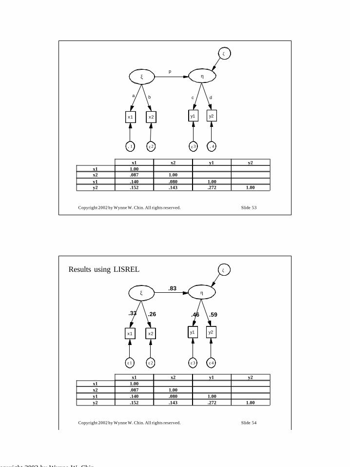
Copyright 2002 by Wynne W. Chin. All rights reserved. Slide 53
x1 x2 y1 y2x1 1.00x2 .087 1.00y1 .140 .080 1.00y2 .152 .143 .272 1.00
p
a b c d
ηξ
x1 x2 y1 y2
,1 ε2 ε3 ,4
ζ
Copyright 2002 by Wynne W. Chin. All rights reserved. Slide 54
.83
.33 .26 .46 .59
ηξ
x1 x2 y1 y2
ε1 ε2 ε3 ε4
ζResults using LISREL
x1 x2 y1 y2x1 1.00x2 .087 1.00y1 .140 .080 1.00y2 .152 .143 .272 1.00

28Copyright 2002 by Wynne W. Chin.
All rights reserved
Copyright 2002 by Wynne W. Chin. All rights reserved. Slide 55
.22
.75 .60 .54 .71
ηξ
x1 x2 y1 y2
ε1 ε2 ε3 ε4
ζ
x1 x2 y1 y2x1 1.00x2 .087 1.00y1 .140 .080 1.00y2 .152 .143 .272 1.00
Results using Partial Least Squares
Copyright 2002 by Wynne W. Chin. All rights reserved. Slide 56
ηξ
Interbatteryfactor analysis (mode A)
29Copyright 2002 by Wynne W. Chin.
All rights reserved
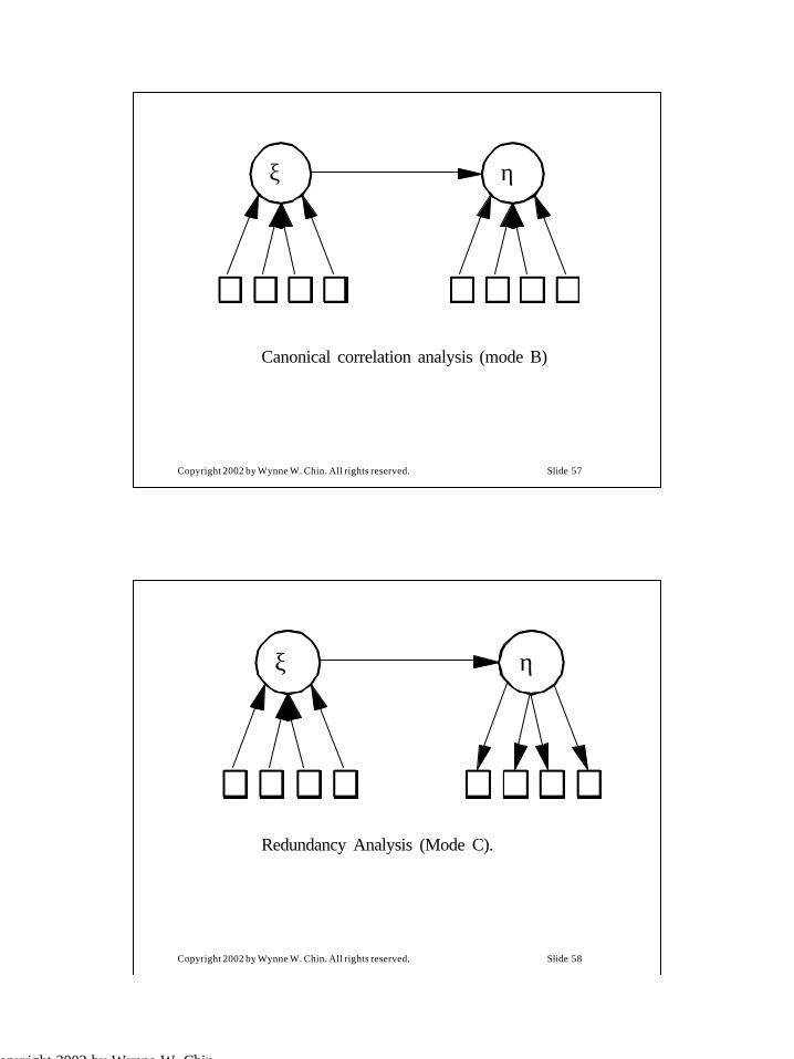
Copyright 2002 by Wynne W. Chin. All rights reserved. Slide 57
Canonical correlation analysis (mode B)
ηξ
Copyright 2002 by Wynne W. Chin. All rights reserved. Slide 58
Redundancy Analysis (Mode C).
ηξ
30Copyright 2002 by Wynne W. Chin.
All rights reserved
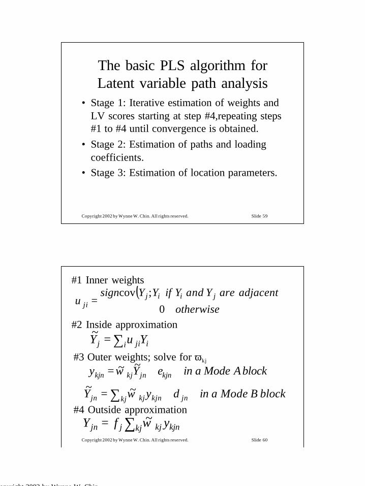
Copyright 2002 by Wynne W. Chin. All rights reserved. Slide 59
The basic PLS algorithm forLatent variable path analysis
• Stage 1: Iterative estimation of weights andLV scores starting at step #4,repeating steps#1 to #4 until convergence is obtained.
• Stage 2: Estimation of paths and loadingcoefficients.
• Stage 3: Estimation of location parameters.
Copyright 2002 by Wynne W. Chin. All rights reserved. Slide 60
( )otherwise
adjacentareYandYifYYsign jiijji 0
;cov=υ
∑= i ijij YY υ~
blockAModeaineYy kjnjnkjkjn += ~~ω
blockBModeaindyY jnkj kjnkjjn += ∑ ω~~
#1 Inner weights
#2 Inside approximation
#3 Outer weights; solve for ωkj
∑= kj kjnkjjjn yfY ω~#4 Outside approximation
31Copyright 2002 by Wynne W. Chin.
All rights reserved
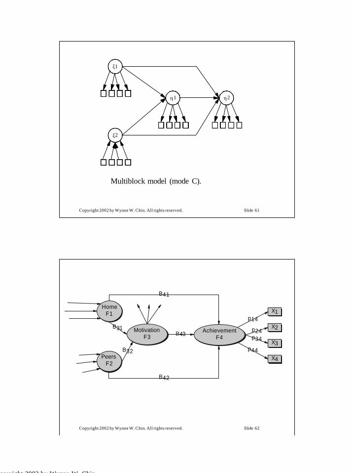
Copyright 2002 by Wynne W. Chin. All rights reserved. Slide 61
ξ1
ξ2
η2η1
Multiblock model (mode C).
Copyright 2002 by Wynne W. Chin. All rights reserved. Slide 62
p14
p24p34
p44
Β43B31
B32
B41
B42
HomeF1
PeersF2
MotivationF3
AchievementF4
X1
X2
X3
X4
32Copyright 2002 by Wynne W. Chin.
All rights reserved
Copyright 2002 by Wynne W. Chin. All rights reserved. Slide 63
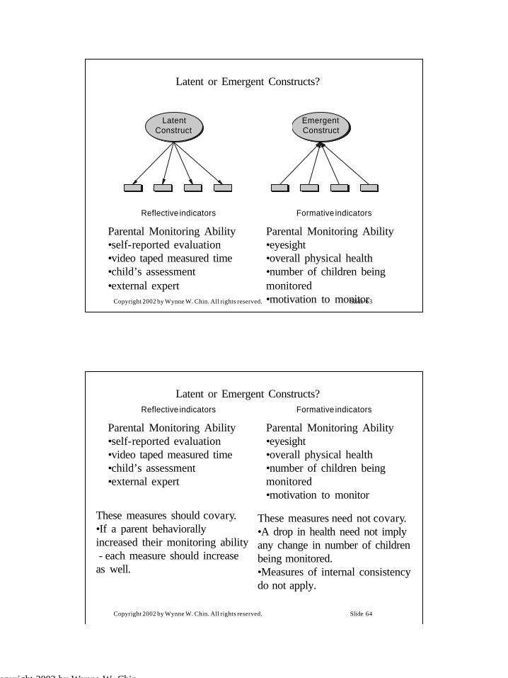
LatentConstruct
EmergentConstruct
Reflective indicators Formative indicators
Latent or Emergent Constructs?
Parental Monitoring Ability•eyesight•overall physical health•number of children beingmonitored•motivation to monitor
Parental Monitoring Ability•self-reported evaluation•video taped measured time•child’s assessment•external expert
Copyright 2002 by Wynne W. Chin. All rights reserved. Slide 64
Reflective indicators Formative indicators
Latent or Emergent Constructs?
Parental Monitoring Ability•eyesight•overall physical health•number of children beingmonitored•motivation to monitor
Parental Monitoring Ability•self-reported evaluation•video taped measured time•child’s assessment•external expert
These measures should covary.•If a parent behaviorallyincreased their monitoring ability- each measure should increaseas well.
These measures need not covary.•A drop in health need not implyany change in number of childrenbeing monitored. •Measures of internal consistencydo not apply.

33Copyright 2002 by Wynne W. Chin.
All rights reserved
Copyright 2002 by Wynne W. Chin. All rights reserved. Slide 65
Test - Latent or Emergent Construct?
Stressful Change Events•Been sexually attacked•Family and parental stress•Accident and illness events•Family relocation events
Mother’s Ability to Interact andMonitor a Child•Number of children in a family•Health of the Mother•Hours of Maternal Employment
Illness•Number of illnesses•Respiratory problems or illnesses•Cardiovascular or circulatory problems
(examples from Cohen, Cohen, Teresi, Marchi, & Velex, 1990)
Copyright 2002 by Wynne W. Chin. All rights reserved. Slide 66
Reflective Items
R1. I have the resources, opportunities and knowledge I would need t o use a databasepackage in my job.
R2. There are no barriers to my using a database package in my job.R3. I would be able to use a database package in my job if I wanted to.R4. I have access to the resources I would need to use a database package in my job.
Formative Items
R5. I have access to the hardware and software I would need to use a database package inmy job.
R6. I have the knowledge I would need to use a database package in my job.R7. I would be able to find the time I would need to use a database package in my job.R8. Financial resources (e.g., to pay for computer time) are not a barrier for me in using a
database package in my job.R9. If I needed someone's help in using a database package in my job, I could get it easily.R10. I have the documentation (manuals, books etc.) I would need to use a database packagein my job.R11. I have access to the data (on customers, products, etc.) I would need to use a database
package in my job.
Table4. The Resource InstrumentFully anchored Likert scales were used. Responses to all items ranged from Extremely likely (7) to Extremely
unlikely (1).

34Copyright 2002 by Wynne W. Chin.
All rights reserved
Copyright 2002 by Wynne W. Chin. All rights reserved. Slide 67
0.539*0.138*
0.433*0.733*
0.045
BehavioralIntention to Use
IT
(R 2 = 0.332)
AttitudeTowards Using
IT
(R2 = 0.668)
Usefulness
(R2 = 0.188)
Ease of Use
Copyright 2002 by Wynne W. Chin. All rights reserved. Slide 68
0.589*(0.930)
0.270*(0.814)
0.100*(0.735)
0.027(0.566)
0.132*(0.654)
-0.022(0.546)
0.118(0.602)
0.873*
0.893*(0.271)
0.904*(0.261)
0.911*(0.274)
0.903*(0.310)
Resourcesformative
Resourcesreflective
R5. Hardware/Software
R6. Knowledge
R7. Time
R8. FinancialResources
R9. Someone'sHelp
R10. Documentation
R11. Data
R1 R2 R3 R4
Figure 7. Redundancy analysis of perceived resources ( * indicates significant estimates).
35Copyright 2002 by Wynne W. Chin.
All rights reserved
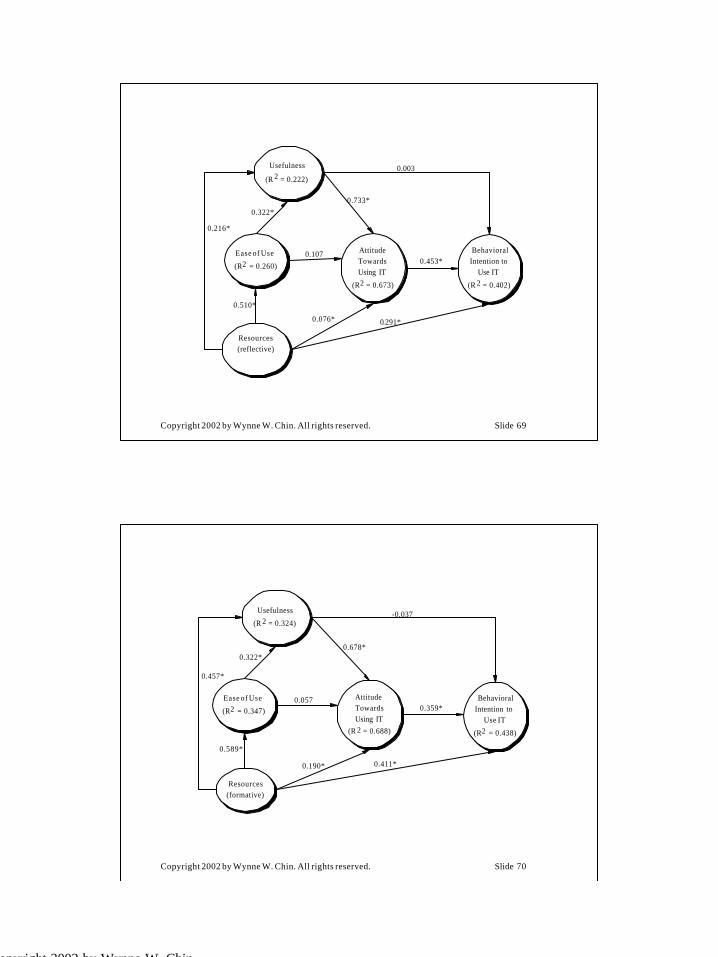
Copyright 2002 by Wynne W. Chin. All rights reserved. Slide 69
0.216*
0.453*0.107
0.322*0.733*
0.003
0.076*
0.510*
0.291*
BehavioralIntention to
Use IT
(R 2 = 0.402)
AttitudeTowardsUsing IT
(R2 = 0.673)
Usefulness
(R 2 = 0.222)
Ease of Use
(R2 = 0.260)
Resources(reflective)
Copyright 2002 by Wynne W. Chin. All rights reserved. Slide 70
0.457*
0.359*0.057
0.322*0.678*
-0.037
0.190*
0.589*
0.411*
BehavioralIntention to
Use IT
(R2 = 0.438)
AttitudeTowardsUsing IT
(R 2 = 0.688)
Usefulness
(R 2 = 0.324)
Ease of Use
(R2 = 0.347)
Resources(formative)
36Copyright 2002 by Wynne W. Chin.
All rights reserved
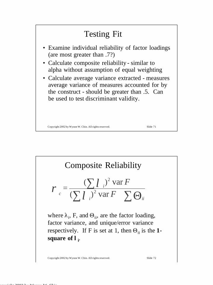
Copyright 2002 by Wynne W. Chin. All rights reserved. Slide 71
Testing Fit• Examine individual reliability of factor loadings
(are most greater than .7?)• Calculate composite reliability - similar to
alpha without assumption of equal weighting• Calculate average variance extracted - measures
average variance of measures accounted for bythe construct - should be greater than .5. Canbe used to test discriminant validity.
Copyright 2002 by Wynne W. Chin. All rights reserved. Slide 72
Composite Reliability
∑Θ∑∑
+=
iii
i
c FF
varvar
2
2
)()(
λλρ
where λi, F, and Θii, are the factor loading,factor variance, and unique/error variancerespectively. If F is set at 1, then Θii is the 1-square of λi.

37Copyright 2002 by Wynne W. Chin.
All rights reserved
Copyright 2002 by Wynne W. Chin. All rights reserved. Slide 73
Average Variance Extracted
∑Θ∑∑
+=
iii
i
F
FAVE
var
var2
2
λλ
where λi, F, and Θii, are the factor loading,factor variance, and unique/error variancerespectively. If F is set at 1, then Θii is the 1-square of λi.
Copyright 2002 by Wynne W. Chin. All rights reserved. Slide 74
Useful Ease of use Resources Attitude Intention
Useful 0.91
Ease of use 0.43 0.83
Resources 0.38 0.51 0.82
Attitude 0.81 0.46 0.41 0.97
Intention 0.48 0.38 0.48 0.58 0.97
Correlation Among Construct Scores (AVE extracted in diagonals).

38Copyright 2002 by Wynne W. Chin.
All rights reserved
Copyright 2002 by Wynne W. Chin. All rights reserved. Slide 75
Loadings and Cross-Loadings for the Measurement (Outer) Model.
USEFUL EASE OFUSE
RESOURCES ATTITUDE INTENTION
U1 0.95 0.40 0.37 0.78 0.48U2 0.96 0.41 0.37 0.77 0.45U3 0.95 0.38 0.35 0.75 0.48U4 0.96 0.39 0.34 0.75 0.41U5 0.95 0.43 0.35 0.78 0.45U6 0.96 0.46 0.39 0.79 0.48
EOU1 0.35 0.86 0.53 0.42 0.35EOU2 0.40 0.91 0.44 0.41 0.35EOU3 0.40 0.94 0.46 0.40 0.36EOU4 0.44 0.90 0.43 0.44 0.37EOU5 0.44 0.92 0.50 0.46 0.36EOU6 0.37 0.93 0.44 0.42 0.33
R1 0.42 0.51 0.90 0.41 0.42R2 0.37 0.50 0.91 0.38 0.46R3 0.31 0.46 0.91 0.35 0.41R4 0.28 0.38 0.90 0.33 0.44A1 0.80 0.47 0.39 0.98 0.54A2 0.80 0.44 0.41 0.99 0.57A3 0.78 0.45 0.41 0.98 0.58I1 0.48 0.38 0.46 0.58 0.97I2 0.47 0.37 0.48 0.56 0.99I3 0.47 0.37 0.48 0.56 0.99
Copyright 2002 by Wynne W. Chin. All rights reserved. Slide 76
Are the results presentedconfirmatory or exploratory?
• If initial exploratory analysis were performed on thesame data set - possible captilization of chance mayoccur.
• Need to provide cross-validation on a new sample.
39Copyright 2002 by Wynne W. Chin.
All rights reserved
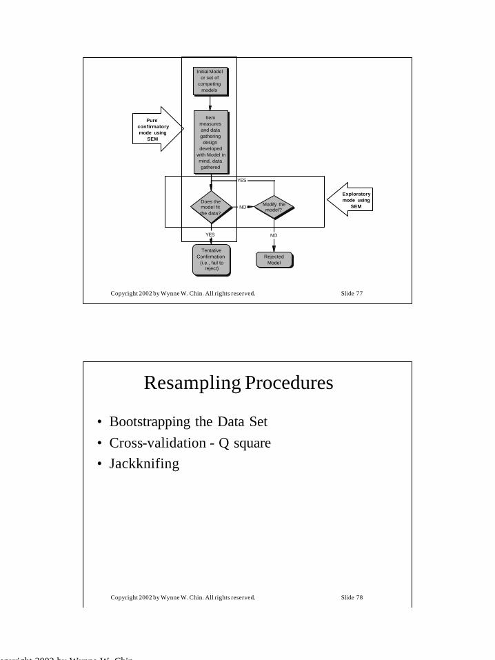
Copyright 2002 by Wynne W. Chin. All rights reserved. Slide 77
YES
NO
YES
NO
Initial Modelor set of
competingmodels
Itemmeasuresand datagathering
designdeveloped
with Model inmind, datagathered
Does themodel fitthe data?
TentativeConfirmation
(i.e., fail toreject)
Modify themodel?
RejectedModel
Exploratorymode using
SEM
Pureconfirmatorymode using
SEM
Copyright 2002 by Wynne W. Chin. All rights reserved. Slide 78
Resampling Procedures
• Bootstrapping the Data Set• Cross-validation - Q square• Jackknifing
40Copyright 2002 by Wynne W. Chin.
All rights reserved
Copyright 2002 by Wynne W. Chin. All rights reserved. Slide 79
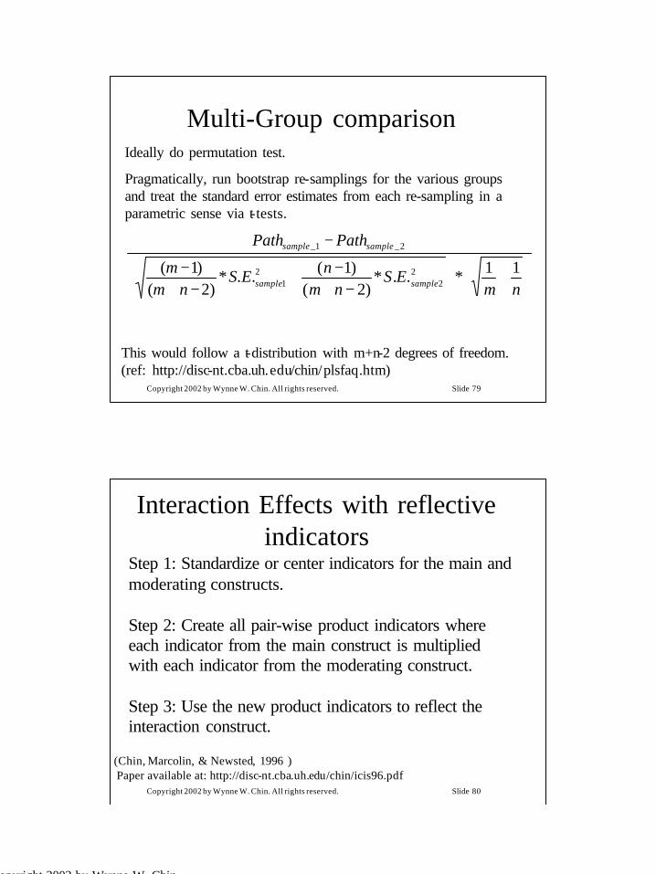
Multi-Group comparisonIdeally do permutation test.
Pragmatically, run bootstrap re-samplings for the various groupsand treat the standard error estimates from each re-sampling in aparametric sense via t-tests.
+
−+
−+−+
−
−
nmES
nmnES
nmm
PathPath
samplesample
samplesample
11*..*)2(
)1(..*)2(
)1( 22
21
2_1_
This would follow a t-distribution with m+n-2 degrees of freedom.(ref: http://disc-nt.cba.uh.edu/chin/plsfaq.htm)
Copyright 2002 by Wynne W. Chin. All rights reserved. Slide 80
Interaction Effects with reflectiveindicators
(Chin, Marcolin, & Newsted, 1996 )Paper available at: http://disc-nt.cba.uh.edu/chin/icis96.pdf
Step 1: Standardize or center indicators for the main andmoderating constructs.
Step 2: Create all pair-wise product indicators whereeach indicator from the main construct is multipliedwith each indicator from the moderating construct.
Step 3: Use the new product indicators to reflect theinteraction construct.

41Copyright 2002 by Wynne W. Chin.
All rights reserved
Copyright 2002 by Wynne W. Chin. All rights reserved. Slide 81
XPredictorVariable
X*ZInteraction
Effect
x1 x2 x3
ZModerator
Variable
z1 z2 z3
YDependent
Variable
y1 y2 y3
x2*z1 x2*z2 x2*z3 x3*z1 x3*z2 x3*z3x1*z1 x1*z2 x1*z3
Copyright 2002 by Wynne W. Chin. All rights reserved. Slide 82
Indicators per constructSample
sizeone item
perconstruct
two perconstruct
(4 forinteraction)
four perconstruct(16 for
interaction)
six perconstruct(36 for
interaction)
eight perconstruct(64 for
interaction)
ten perconstruct(100 for
interaction)
twelve perconstruct(144 for
interaction)
20 0.1458(0.2852)
0.1609(0.3358)
0.2708(0.3601)
0.1897(0.4169)
0.1988(0.4399)
0.2788(0.3886)
0.3557(0.3725)
50 0.1133(0.1604)
0.1142(0.2124)
0.2795(0.1873)
0.2403(0.2795)
0.3066(0.2183)
0.3083(0.2707)
0.3615(0.1848)
100 0.1012(0.0989)
0.1614(0.1276)
0.2472(0.1270)
0.2669 (0.1301)
0.3029(0.0916)
0.3029(0.0805)
0.3008 (0.1352)
150 0.0953(0.0843)
0.1695 (0.0844)
0.2427(0.0778)
0.2834(0.0757)
0.2805(0.0916)
0.3040(0.0567)
0.2921(0.0840)
200 0.0962(0.0785)
0.1769(0.0674)
0.2317(0.0543)
0.2730(0.0528)
0.2839(0.0606)
0.2843(0.0573)
0.3018(0.0542)
500 0.0965 (0.0436)
0.1681(0.0358)
0.2275(0.0419)
0.2448(0.0379)
0.2637(0.0377)
0.2659(0.0353)
0.2761(0.0375)
Results from Monte Carlo Simulation

42Copyright 2002 by Wynne W. Chin.
All rights reserved
Copyright 2002 by Wynne W. Chin. All rights reserved. Slide 83
Factor LoadingPatterns for 8 items -pattern repeated for
both X and Zconstructsa
PLS ProductIndicator Estimatesb
Regression EstimatesUsing Averaged
Scoresb
4 at .802 at .702 at.60
x*z--> y 0.307(0.0970)
x*z--> y 0.2562(0.0831)
4 at .804 at .70
x*z--> y 0.3043(0.0957)
x*z--> y 0.2646(0.0902)
4 at .804 at .60
x*z--> y 0.3052(0.1004)
x*z--> y 0.2542(0.0795)
4 at .802 at .602 at .40
x*z--> y 0.3068(0.0969)
x*z--> y 0.2338(0.0801)
6 at .802 at .40
x*z--> y 0.3012(0.1048)
x*z--> y 0.2461(0.0886)
4 at .704 at.60
x*z--> y 0.2999(0.1277)
x*z--> y 0.2324(0.0806)
4 at.702 at .602 at .30
x*z--> y 0.3193(0.1298)
x*z--> y 0.2209(0.0816)
The Impact of Heterogeneous Loadings on the Interaction Estimate(PLS vs. Regression – sample size = 100)
Copyright 2002 by Wynne W. Chin. All rights reserved. Slide 84
Interaction with formative indicators
Follow a two step construct score procedure.
Step 1: Use the formative indicators inconjunction with PLS to create underlyingconstruct scores for the predictor and moderatorvariables.
Step 2: Take the single composite scores fromPLS to create a single interaction term.
Caveat: This approach has yet to be tested in a Monte Carlo simulation.
43Copyright 2002 by Wynne W. Chin.
All rights reserved
Copyright 2002 by Wynne W. Chin. All rights reserved. Slide 85
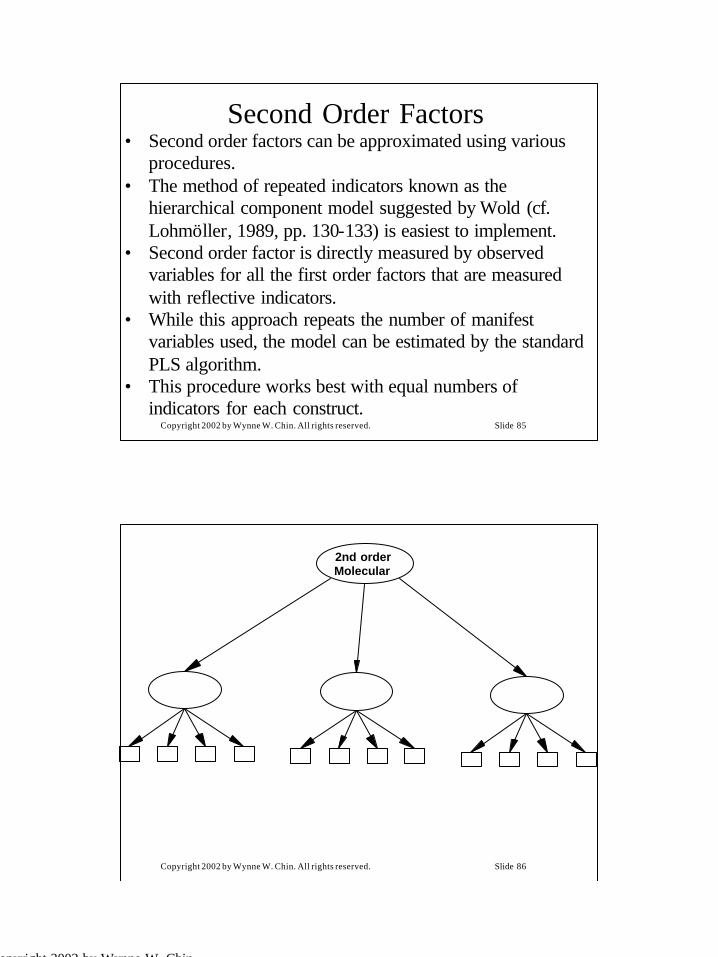
Second Order Factors• Second order factors can be approximated using various
procedures.• The method of repeated indicators known as the
hierarchical component model suggested by Wold (cf.Lohmöller, 1989, pp. 130-133) is easiest to implement.
• Second order factor is directly measured by observedvariables for all the first order factors that are measuredwith reflective indicators.
• While this approach repeats the number of manifestvariables used, the model can be estimated by the standardPLS algorithm.
• This procedure works best with equal numbers ofindicators for each construct.
Copyright 2002 by Wynne W. Chin. All rights reserved. Slide 86
2nd orderMolecular
44Copyright 2002 by Wynne W. Chin.
All rights reserved
Copyright 2002 by Wynne W. Chin. All rights reserved. Slide 87
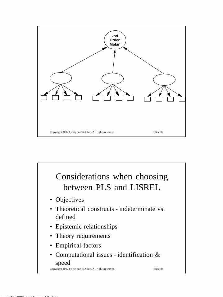
2ndOrderMolar
Copyright 2002 by Wynne W. Chin. All rights reserved. Slide 88
Considerations when choosingbetween PLS and LISREL
• Objectives• Theoretical constructs - indeterminate vs.
defined• Epistemic relationships• Theory requirements• Empirical factors• Computational issues - identification &
speed

45Copyright 2002 by Wynne W. Chin.
All rights reserved
Copyright 2002 by Wynne W. Chin. All rights reserved. Slide 89
Objectives
• Prediction versus explanation
Copyright 2002 by Wynne W. Chin. All rights reserved. Slide 90
Theoretical constructs -Indeterminate versus defined
• For PLS - the latent variables are estimatedas linear aggregates or components. Thelatent variable scores are estimated directly. If raw data is used, scoring coefficients areestimated.
• For LISREL - Indeterminacy

46Copyright 2002 by Wynne W. Chin.
All rights reserved
Copyright 2002 by Wynne W. Chin. All rights reserved. Slide 91
Epistemic relationships
• Latent constructs with reflective indicators -LISREL & PLS
• Emergent constructs with formativeindicators - PLS
• By choosing different weighting “modes”the model builder shifts the emphasis of themodel from a structural causal explanationof the covariance matrix to aprediction/reconstruction forecast of the rawdata matrix
Copyright 2002 by Wynne W. Chin. All rights reserved. Slide 92
Theory requirements
• LISREL expects strong theory(confirmation mode)
• PLS is flexible

47Copyright 2002 by Wynne W. Chin.
All rights reserved
Copyright 2002 by Wynne W. Chin. All rights reserved. Slide 93
Empirical factors
• Distributional assumptions– PLS estimation is a “rigid” technique that
requires only “soft” assumptions about thedistributional characteristics of the raw data.
– LISREL requires more stringent conditions.
Copyright 2002 by Wynne W. Chin. All rights reserved. Slide 94
Empirical factors (continued)• Sample Size depends on power analysis, but
much smaller for PLS– PLS heuristic of ten times the greater of the
following two (ideally use power analysis)• construct with the greatest number of formative
indicators• construct with the greatest number of structural paths
going into it
– LISREL heuristic - at least 200 cases or 10 timesthe number of parameters estimated.
48Copyright 2002 by Wynne W. Chin.
All rights reserved
Copyright 2002 by Wynne W. Chin. All rights reserved. Slide 95
Empirical factors (continued)• Types of measures
– PLS can use categorical through ratio measures– LISREL generally expects interval level,
otherwise need PRELIS preprocessing.
Copyright 2002 by Wynne W. Chin. All rights reserved. Slide 96
Computational issues -Identification
• Are estimates unique?• Under recursive models - PLS is always
identified• LISREL - depends on the model. Ideally
need 4 or more indicators per construct tobe over determined, 3 to be just identified.Algebraic proof for identification.
49Copyright 2002 by Wynne W. Chin.
All rights reserved
Copyright 2002 by Wynne W. Chin. All rights reserved. Slide 97
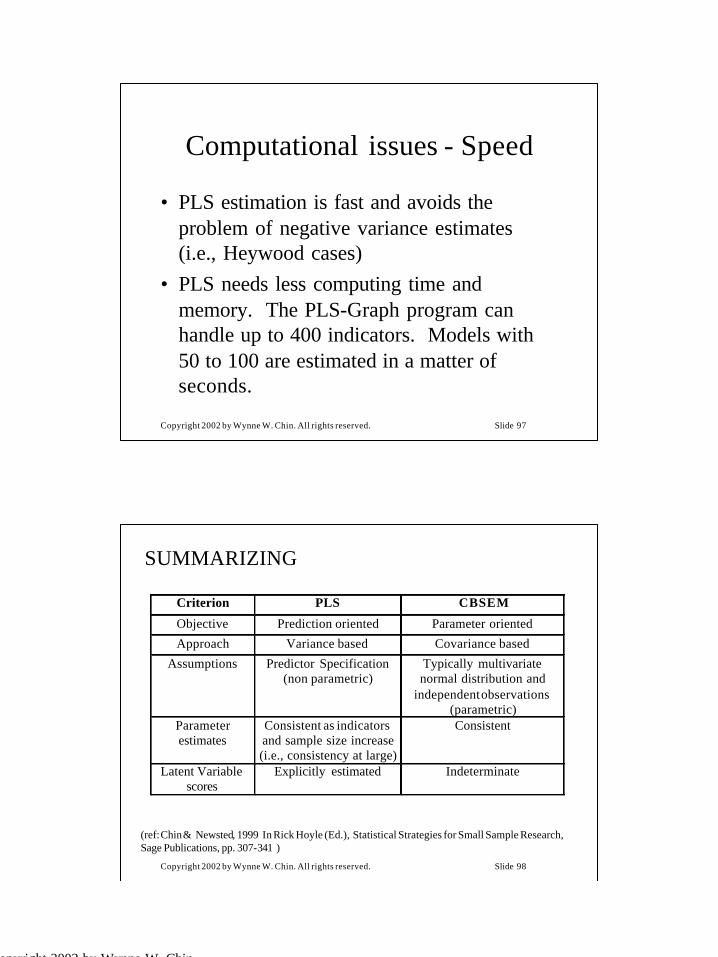
Computational issues - Speed
• PLS estimation is fast and avoids theproblem of negative variance estimates(i.e., Heywood cases)
• PLS needs less computing time andmemory. The PLS-Graph program canhandle up to 400 indicators. Models with50 to 100 are estimated in a matter ofseconds.
Copyright 2002 by Wynne W. Chin. All rights reserved. Slide 98
Criterion PLS CBSEM
Objective Prediction oriented Parameter oriented
Approach Variance based Covariance based
Assumptions Predictor Specification(non parametric)
Typically multivariatenormal distribution and
independent observations(parametric)
Parameterestimates
Consistent as indicatorsand sample size increase(i.e., consistency at large)
Consistent
Latent Variablescores
Explicitly estimated Indeterminate
(ref: Chin & Newsted, 1999 In Rick Hoyle (Ed.), Statistical Strategies for Small Sample Research,Sage Publications, pp. 307-341 )
SUMMARIZING

50Copyright 2002 by Wynne W. Chin.
All rights reserved
Copyright 2002 by Wynne W. Chin. All rights reserved. Slide 99
Criterion PLS CBSEM
Epistemicrelationship
between a latentvariable and its
measures
Can be modeled in eitherformative or reflective
mode
Typically only withreflective indicators
Implications Optimal for predictionaccuracy
Optimal for parameteraccuracy
ModelComplexity
Large complexity (e.g.,100 constructs and 1000
indicators)
Small to moderatecomplexity (e.g., less than
100 indicators)
Sample SizePower analysis based onthe portion of the modelwith the largest numberof predictors. Minimalrecommendations range
from 30 to 100 cases.
Ideally based on poweranalysis of specific model -minimal recommendations
range from 200 to 800.
(ref: Chin & Newsted, 1999 In Rick Hoyle (Ed.), Statistical Strategies for Small Sample Research,Sage Publications, pp. 307-341 )
SUMMARIZING
Copyright 2002 by Wynne W. Chin. All rights reserved. Slide 100
Additional Questions?


![Taking Stress Out of Stressful Conversations[1]](https://static.fdocuments.in/doc/165x107/544ccfd0b1af9f67018b4c7f/taking-stress-out-of-stressful-conversations1.jpg)