Partial Frequency Reuse for Long Term Evolution - TU … Partial Frequency Reuse for Long Term...
110
DISSERTATION Partial Frequency Reuse for Long Term Evolution ausgef¨ uhrt zum Zwecke der Erlangung des akademischen Grades eines Doktors der technischen Wissenschaften unter der Leitung von Prof. Christoph F. Mecklenbr¨ auker Institute of Telecommunications eingereicht an der Technischen Universit¨ at Wien Fakult¨ at f¨ ur Elektrotechnik von Bujar Krasniqi Wien, im December 2011
Transcript of Partial Frequency Reuse for Long Term Evolution - TU … Partial Frequency Reuse for Long Term...

DISSERTATION
Partial Frequency Reuse
for Long Term Evolution
ausgefuhrt zum Zwecke der Erlangung des akademischen Grades eines
Doktors der technischen Wissenschaften
unter der Leitung von
Prof. Christoph F. Mecklenbrauker
Institute of Telecommunications
eingereicht an der Technischen Universitat Wien
Fakultat fur Elektrotechnik
von
Bujar Krasniqi
Wien, im December 2011


Die Begutachtung dieser Arbeit erfolgte durch:
1. Prof. Christoph F. Mecklenbrauker
Institute of Telecommunications
Technische Universitat Wien
2. Prof. Erik G. Strom
Department of Signals and Systems
Chalmers University


to my family

Abstract
In this thesis, I propose, develop, and analyze novel optimization techniques which solve
resource allocation problems in partial frequency reuse (PFR) networks. In long term
evolution (LTE), multiple access in the downlink is established by Orthogonal Fequency
Division Multiple Access (OFDMA). As a consequence, the cell edge users suffer from
strong inter cell interference (ICI). This effect becomes even more severe, due to the
low signal power which the cell edge users receive from the base station. Therefore, in
this work, we have formulated algorithms that mitigate the ICI by optimizing the Radio
Resource Allocation (RRA).
An efficient use of radio resources (bandwidth and transmit power) is indispensable,
since they are expensive and limited by spectrum licenses. For Inter Cell Interference
(ICI) reduction, we define Partial Frequency Reuse (PFR) such that frequency reuse-
1 is allocated to center-cell users and frequency reuse-3 is allocated to cell-edge users.
Near the cell edges, the Orthogonal Frequency Division Multiplexing (OFDM) sub-carriers
are allocated such that the users within do not use the same frequencies simultaneously
(frequency reuse-3). We note that some bandwidth remains unused if the users spatial
distribution is inhomogeneous in the cell. In this case, such a PFR scheme does not
lead to an efficient utilization of radio resources. To mitigate this apparent inefficiency, I
propose a novel bandwidth re-allocation scheme by maximizing the cell capacity density
(i.e. achievable data rate per bandwidth per unit area). The proposed scheme re-allocates
bandwidth from the cell edge to the center of the cell. The cell capacity density is a
metric that represents the expected capacity per unit area for a randomly positioned
user (uniformly distributed) in the cell. The network operators are interested in the
achievable transmission rate per user. Therefore, we formulate the optimization problem
as a maximization of the sum-rate under power and bandwidth constraints. We proved that
this sum-rate maximization problem becomes convex for a fixed PFR bandwidth allocation
scheme under a suitable additional power equality constraint. Using the Lagrangian, the
analytical solutions are derived for the optimal power allocation, in a manner which is
closely related to water-filling. Furthermore, we formulated two specific problems for the
joint optimization of power and bandwidth allocation as convex geometric programs, i.e.
the maximization of the minimum rate and the sum-power minimization, respectively.
vii
viii
In PFR, a fundamental issue is to classify the users to the cell edge and center-cell
regions. Two user classification schemes are investigated in this thesis in detail: The
first classification scheme is based on the distance between the user and its serving base
station. The second classification scheme is based on the users Large-Scale Path-Loss
Attenuation (LSPLA). Compared to the first classification scheme, the LSPLA scheme is
proved to enhance the achievable user-rates. We have shown that the LSPLA classification
scheme is successfully applicable to all discussed problems. Finally, we conclude that the
LSPLA scheme allows us to formulate spectrally efficient RRA algorithms in a form which
can be implemented with fairly low numerical complexity.

Kurzfassung
In dieser Arbeit prasentiere ich die Entwicklung und Analyse neuer Optimierungstech-
niken, mit deren Hilfe das Problem der Aufteilung begrenzter Betriebsmittel in zellularen
Kommunikationsnetzen mit teilweiser Frequenz-Wiederverwendung (engl. partial frequency
reuse (PFR)) gelost werden kann. Gemaß dem Mobilfunkstandard der vierten Generation
(4G), bekannt unter dem Akronym LTE (long term evolution), wird der Vielfachzugriff auf
den Funkkanal in der Abwartsstrecke durch das Verfahren des orthogonalen Frequenzmul-
tiplexzugriffs (engl. orthogonal frequency division multiple (OFDM) access (OFDMA))
realisiert. Dies hat zur Folge, dass die Empfangsqualitat in den Geraten der Netzteil-
nehmer nahe der Zellgrenzen stark durch die von den Nachbarzellen verursachten Inter-
ferenezen (engl. inter cell interference (ICI)) beeintrachtigt wird. Aus dieser Motivation
heraus formulieren wir in dieser Arbeit Algorithmen zur Optimierung der Funkbetriebs-
mittelzuweisung (engl. radio resource allocation (RRA)), die es erlauben den negativen
Einfluss durch ICI wesentlich zu reduzieren.
Spektrumslizenzen und Energiekosten machen die effiziente Nutzung der Betriebsmittel
(spektrale Bandbreite und Sendeleistung) in drahtlosen Kommunikationsnetzen unabding-
bar. Mit dem Ziel der Reduktion von ICI definieren wir PFR so, dass den Netzteilnehmern
in den Kerngebieten aller Zellen die gleichen Frequenzbander zur Verfugung stehen. In
den Bereichen nahe der Zellgrenzen werden die zuweisbaren OFDM Teiltrager hinge-
gen so eingeschrankt, dass Netzteilnehmer benachbarter Zellen unter keinen Umstanden
die gleichen Frequenzen benutzen konnen. Die in den Kerngebieten genutzte Frequenz-
aufteilungsstrategie wird in der Literatur haufig mit frequency reuse-1 (deu. Frequenz
Wiederverwendung-1) bezeichnet, jene fur die Bereiche nahe der Zellgrenzen mit frequency
reuse-3 (deu. Frequenz Wiederverwendung-3). An dieser Stelle sei darauf hingewiesen,
dass die hier gewahlte PFR Methode keine optimale Nutzung der spektralen Ressourcen
erlaubt, wenn die raumliche Verteilung der Netzteilnehmer in den Zellen ungleichmaßig
ist. Um dieser offensichtlichen Ineffizienz zu begegnen, fuhre ich ein neues Verfahren ein,
das es in jeder Zelle erlaubt Teilbander je nach Bedarf entweder dem Kerngebiet oder
dem grenznahen Bereich zuzuordnen. Auf diese Weise kann die Dichte der Zellkapazitat,
die ein flachenbezogenes Maß fur die erwartete Kapazitat eines im gesamten Zellgebiet
gleichermaßen wahrscheinlich positionierten Netzteilnehmers ist, maximiert werden. Die
ix
x
Netzbetreiber sind an der erzielbaren Ubertragungsrate pro Netzteilnehmer interessiert.
Aus diesem Grund entwickeln wir die hier prasentierten Verfahren durch die Formulierung
von Optimierungsproblemen, die die Gesamtubertragungsrate aller Netzteilnehmer maxi-
mieren und zusatzlich erlauben die Begrenztheit von Bandbreite und Sendeleistung in
Form von Nebenbedingungen zu berucksichtigen. Fur PFRmit fixer Bandbreitenzuweisung
und unter der Annahme gleicher Gesamtsendeleisung aller Zellen, konnten wir zeigen,
dass das entsprechende Optimierungsproblem konvex ist. Mit Hilfe der Lagrangefunktion
gelingt es uns, fur dieses Problem eine geschlossene Losung anzugeben, die der Metho-
de des Water-Filling ahnelt und eine optimale Leistungsaufteilung garantiert. Daruber
hinaus formulieren wir das Problem der gemeinsamen Optimierung von Sendeleistung
und Bandbreitenzuweisung fur zwei spezielle Falle. Im einen Fall wird die minimale
Ubertragungsrate maximiert, im anderen Fall wird die Gesamtsendeleistung minimiert.
Beide Varianten lassen sich in Optimierungsprobleme der bekannten Form eines konvexen
geometrischen Programms uberfuhren.
Um PFR einsetzen zu konnen mussen in jeder Zelle alle Netzteilnehmer einer von
zwei disjunkten Gruppen zugeordnet werden – dies ist einerseits die Gruppe der Netz-
teilnehmer im Kerngebiet der Zelle, und andererseits die Gruppe der Netzteilnehmer
nahe der Zellgrenze. In dieser Arbeit untersuchen wir zwei Methoden um die Netzteil-
nehmer zu klassifizieren. Das erste Verfahren nimmt die Zuordnung der Nutzer basierend
auf deren geschatzter Distanz zur Basisstation vor. Das zweite Verfahren verwendet
statt der Distanz die großraumige Streckendampfung (engl. large-scale path-loss atten-
uation (LSPLA)). Der Vergleich beider Verfahren zeigt, dass das zweite Verfahren zu
hoheren erzielbaren Ubertragungsraten fuhrt. Außerdem zeigen wir, dass die LSPLA-
basierte Klassifizierungsmethode in allen betrachteten Problemfallen eingesetzt werden
kann. Wir kommen zu dem Schluss, dass es diese Klassifizierungsmethode ermoglicht
spektral effiziente RRA Algorithmen anzugeben, die sich mit verhaltnismaßig geringer
numerischer Komplexitat implementieren lassen.
Acknowledgments
First and foremost, I wish to express my deepest gratitude to my supervisor Christoph
Mecklenbrauker. It was really a great experience to work with him during my PhD studies.
He was always motivating me with his enthusiasm. He actively contributed to my research
with new ideas and guidance. It was my pleasure to participate with him in various events
at several Cost Meetings (COST Action 2100 and IC1004). Additionally, I would like to
express my gratitude to my second examiner Erik Strom for his patience in awaiting the
final version of this thesis. I also appreciate the fruitful discussions that we had in Miami
during the IEEE GLOBECOM 2010 conference and at some Cost Meetings (COST Action
2100 and IC1004).
I would like to express my gratitude to Joachim Wehinger for his support and advise
during the time that I was as visiting researcher at Telecommunications Research Center
Vienna. Furthermore I would like to thank my colleges and co-authors Martin Wrulich,
Martin Wolkerstorfer, Christian Mehlfuhrer, and Markus Rupp for their strong support
which often brought me to new insights. This thank extends to Robert Dallinger, Aamir
Habib, Markus Laner, Jesus Gutierrez Teran, Stefan Schwarz and Martin Mayer who
carefully proofread chapters of my thesis. I also would like to thank all the other colleagues
from our institute with whom I shared the time during my PhD studies.
Special thanks go to Driton Statovci for his guidance, continuous support and useful
suggestions as well as motivating me to keep the work ongoing. I would like to thank
also Nysret Musliu who recommended to do my PhD studies at Vienna University of
Technology. I am grateful to Myzafere Limani and Enver Hamiti from University of
Prishtina who gave a contribution in this aspect.
Especially, I would like to thank my wife Luljeta and my daughter Laura who encour-
aged and supported me during writing this thesis. Their patience during the last months
was an inspiration and gave me energy for finishing this work in time.
Finally, I would like to thank my parents, my father Ismet and my mother Elmije
who always motivated me to do the PhD, as well as my brothers Behar and Besnik who
encouraged me during all this time.
xi


Contents
1 Introduction 1
2 Radio Resource Management — an Overview 52.1 Radio Resource Management / Long Term Evolution . . . . . . . . . . . . . . 6
3 Optimization Techniques for RRM in Wireless Commu-nications 93.1 Dual Decomposition Techniques for Wireless Communications . . . . . . . . . 10
3.1.1 The Lagrangian of an Optimization Problem . . . . . . . . . . . . . . 10
3.1.2 KKT optimality conditions . . . . . . . . . . . . . . . . . . . . . . . . 11
3.2 Geometric Programming for Wireless Communications . . . . . . . . . . . . . 12
3.2.1 Geometric Programming in Basic Form . . . . . . . . . . . . . . . . . 12
3.2.2 Transformation of the GGP to GP and its form in CVX . . . . . . . . . 13
4 Capacity Density Maximization for LTE 154.1 Geometry of Cell Cluster Model . . . . . . . . . . . . . . . . . . . . . . . . . . 16
4.1.1 Path-loss Exponent Model . . . . . . . . . . . . . . . . . . . . . . . . 17
4.1.2 Average Received SINR . . . . . . . . . . . . . . . . . . . . . . . . . . 17
4.2 Frequency Reuse Schemes . . . . . . . . . . . . . . . . . . . . . . . . . . . . . 19
4.3 Capacity density for Partial Frequency Reuse . . . . . . . . . . . . . . . . . . . 21
5 Power Allocation in Partial Frequency Reuse 255.1 Geometry of Cell Cluster Model . . . . . . . . . . . . . . . . . . . . . . . . . . 26
5.2 Large-scale Path-loss Attenuation . . . . . . . . . . . . . . . . . . . . . . . . . 28
5.2.1 Antenna Gain . . . . . . . . . . . . . . . . . . . . . . . . . . . . . . . 28
5.2.2 Penetration Loss . . . . . . . . . . . . . . . . . . . . . . . . . . . . . . 29
5.2.3 Shadowing . . . . . . . . . . . . . . . . . . . . . . . . . . . . . . . . . 30
5.2.4 Small-scale Fading . . . . . . . . . . . . . . . . . . . . . . . . . . . . 30
xiii

xiv
5.3 Variable Power and Fixed Bandwidth Allocation Scheme . . . . . . . . . . . . 30
5.4 Power Allocation Algorithm . . . . . . . . . . . . . . . . . . . . . . . . . . . . 31
5.4.1 Water-filling Like Power Allocation . . . . . . . . . . . . . . . . . . . . 33
5.5 Power Allocation Algorithms in Convex Form . . . . . . . . . . . . . . . . . . 37
5.5.1 Maximization of the Minimum Rate in Convex Form . . . . . . . . . . 37
5.5.2 Sum-Power Minimization in Convex Form . . . . . . . . . . . . . . . . 38
6 Bandwidth and Power Allocation in Partial FrequencyReuse 416.1 Variable Power and Variable Bandwidth Allocation Scheme . . . . . . . . . . . 42
6.2 Bandwidth and Power Allocation Algorithms . . . . . . . . . . . . . . . . . . . 43
6.2.1 Maximization of the Minimum Rate . . . . . . . . . . . . . . . . . . . 43
6.2.2 Efficient Algorithms for Bandwidth and Power Allocation Depending
on Users Classification . . . . . . . . . . . . . . . . . . . . . . . . . . 50
6.3 Bandwidth Re-allocation Scheme . . . . . . . . . . . . . . . . . . . . . . . . . 55
6.3.1 Power Allocation and Bandwidth Re-Allocation Depending on Distance
from Base Station . . . . . . . . . . . . . . . . . . . . . . . . . . . . . 56
6.3.2 Power Allocation and Bandwidth Re-allocation Depending on Large-
scale Path-loss Attenuations . . . . . . . . . . . . . . . . . . . . . . . 60
6.4 Power Allocation and Bandwidth Adaptation Algorithms . . . . . . . . . . . . 64
6.4.1 Optimal power and adaptive bandwidth allocation depending on mean
LSPLA . . . . . . . . . . . . . . . . . . . . . . . . . . . . . . . . . . . 65
6.4.2 Efficient power and adaptive bandwidth algorithm depending on mean
LSPLA . . . . . . . . . . . . . . . . . . . . . . . . . . . . . . . . . . . 72
7 Conclusions 777.1 Capacity Density Maximization . . . . . . . . . . . . . . . . . . . . . . . . . . 78
7.2 Power Allocation in Partial Frequency Reuse . . . . . . . . . . . . . . . . . . . 78
7.3 Bandwidth and Power Allocation in Partial Frequency Reuse . . . . . . . . . . 78
8 Future Directions / Outlook 81
List of Symbols 83
List of Acronyms 87
List of Figures 89
Bibliography 91
1Introduction
HIGHER transmission data rate required by mobile users is a big challenge that need
to be considered. Nowadays, the mobile handsets called smartphones are capable of
supporting higher communication speeds as the notebooks can do. In order to address the
issue of requirement for higher transmission speed, new generation of mobile communi-
cation networks are standardized like Wireless Local Area Network (WLAN), Worldwide
Interoperability for Microwave Access (WiMAX), Long Term Evolution (LTE) and Long
Term Evolution-Advanced (LTE-A), that offer higher transmission rate compared with
Universal Mobile Telecommunications System (UMTS). Such networks use OFDMA as
multiple access scheme in the downlink that offers flexibility in bandwidth allocation.
However, because of the use of OFDMA the ICI becomes a limiting factor in achieving
higher capacity [1]. In order to deal with ICI issue, the development of more advanced
frequency allocation schemes is necessary. Considering the fact that bandwidth resources
are limited, it is necessary formulating the efficient optimization algorithms suitable for
optimization the resource allocation. This would allow the mobile operators to use the
bandwidth resources efficiently while satisfying the user’s demands.
Until now several frequency allocation schemes have been proposed for LTE that try
to reduce the ICI and increase the transmission rate. One of those schemes which seems to
be most promising technique is PFR. A number of publication associated with numerical
and simulation results about PFR are shown by authors in [2], [3], [4], [5], [6]. The
PFR splits the bandwidth allocation into two parts: the Full Reuse (FR) part and the
Partial Reuse (PR) part. For the cell center users the PFR allocates the FR part of
the bandwidth, while for the cell edge users it allocates the PR part of the bandwidth.
Other investigations like PFR scheme in combination with Soft Handover (SH) is done
by Chiu et al. [3], where a significant improvement in the throughput for the PR region
1
2 Chapter 1. Introduction
is achieved. At the same time a decrease in the throughput of the FR region is noticed,
because the resources in FR region are shared with the users in the PR region. A solution
for the frequency partitioning radius in PFR through the optimization of the capacity
density is done by Alsawah et al. [6], where he has found an improvement in capacity
density applying PFR compared with applying reuse-1 or reuse-3. Xiang et al. [4] and
Chiu et al. [3] have mentioned that cell edge bandwidth can be re-used by cell center users
whenever the cell edge users are idle. Cell Capacity density maximization together with
frequency bandwidth re-allocation for PFR is studied by Krasniqi et al. [7].
The cellular network users are willing to pay for the transmission rate that mobile
operators are going to offer. So to satisfy the user’s requirements for transmission rate
with the resources that mobile operators have, further investigations differently from the
definition of cell capacity density are carried out. Those investigations are focused on
the optimization algorithms for power and bandwidth allocation. Such algorithms are
in general non-convex because of the interference term in the Signal-to-Interference-and-
Noise-Ratio (SINR) definition. During the last years many optimization algorithms have
been developed for mobile networks that use frequency reuse-1. One of them is the optimal
power allocation for two base station, employing the scheduling schemes under frequency
reuse-1 that is studied by Gjendemsjo et al. [8]. Additionally to the power control in
sum-rate maximization for reuse-1 network, the maximization of the minimum rate for
two users is studied by Charafeddine et al. [9]. The optimal power allocation together
with the minimum rate constraints per cell is studied by Chen et al. [10]. The sum-
rate maximization under variable power control for two users, using sequential geometric
programming is studied by Charafeddine et al. [11]. Differently from frequency reuse-
1 the sum-rate maximization problem for power and bandwidth allocation in PFR is
investigated by Krasniqi et al. [12]. Using the Dual Decomposition Techniques (DDT)
analytical expressions for optimal power allocation within cell regions are derived. Further
study of sum-rate maximization together with bandwidth re-allocation is done by Krasniqi
et al. [13]. Under the assumption of the equal power allocation over all cells in the cluster,
it was shown that the non-convex sum-rate maximization problem can be converted into
convex one. For more than two users this optimization problem was found to be intractable
for analytical solutions.
Differently from the sum-rate maximization problems in the study made by Chiang
et al. [14], the two problems for single carrier power control: maximization the minimum
rate and the sum-power minimization over multiple users within multiple cells for Code
Division Multiple Access (CDMA) networks, was found to be transformable into Geometric
Programming (GP) optimization problems in the high-SINR regime. The maximization
of the minimum rate and the sum-power minimization for multiple users over multiple
cells in PFR are investigated in [12] where without making any high-SINR approximation
Chapter 1. Introduction 3
is proved that those optimization problems can be converted into GP convex ones.
A frequency reuse technique as combination of power allocation and interference aware
for achieving better coverage and higher spectral efficiency is investigated by Xie et al. [15].
A differentiable spectrum partitioning where the reuse distance is used to find the fre-
quency reuse-factors is studied by Fu et al. [16]. Differently from [16] the efficient op-
timization algorithms based on maximization of the minimum rate are developed, that
jointly optimizes the power and bandwidth allocation. Using the efficient algorithms de-
veloped by Krasniqi et al. [17], it is proven that considering the mean LSPLA as threshold
for user’s classification in the cell regions, the PFR becomes more efficient in power al-
location than reuse-1 and reuse-3 for the same minimum rate constraints. Furthermore,
using the LSPLA as threshold to classify the users, two other algorithms for power allo-
cation and bandwidth adaption are developed. Those algorithms adapts the bandwidth
allocation in the cell regions based on the amount of users classified by LSPLA threshold,
and optimize the power allocation.
During my research work I published several papers as the first author and as co-
author. Most of the content from the papers that I am as first author is included in
my thesis. In [7] a novel frequency bandwidth re-allocation is presented and capacity
density maximization is formulated for that scheme. In [12] an optimization problem for
RRA is formulated where for fixed bandwidth allocation, analytical expressions are de-
rived for power allocation. The analytical expressions are applied with the bandwidth
re-allocation [13], [18]. Also in [19] a significant gain in the sum-rate is achieved applying
the optimal power allocations algorithm when LSPLA threshold is used compared with
use of distance threshold. The efficient power allocation and optimal bandwidth allocation
problem formulated by maximization of the minimum rate is shown in [17]. Considering
the maximization of the minimum rate as the optimization problem for power and band-
width allocation in [20] the efficient algorithms for user’s classification and radio resource
allocation are developed.
The following chapters after introduction are organized as follows. In Chapter 2 a
detailed description of RRA and Radio Resource Management (RRM) techniques for LTE
are explained. Also a detailed description of the radio interface architecture implemented
in LTE is shown in this chapter. In Chapter 3 two optimization techniques necessary
to formulate and solve optimization problems for RRA are explained. Those include
the DDT and the GP applicable to wireless communication systems. In Chapter 4 cell
capacity density maximization is shown. Also the novel frequency bandwidth re-allocation
is presented in this chapter where an application of this scheme to improve the capacity
density is presented. In Chapter 5, the optimal power allocation algorithms are derived.
Two models for cell clusters that contains all the parameters which characterize the wireless
channel in the downlink (form the base station to the mobile station) are presented in this

4 Chapter 1. Introduction
chapter. Furthermore, in this chapter the non-convex GP optimization problems of radio
resource allocation are transformed into GP convex optimization problems. In Chapter 6,
efficient algorithms are presented to classify the users in the cell regions. Moreover, in
this chapter efficient power and adaptive bandwidth allocation and also optimal power
and adaptive bandwidth allocation algorithms are developed. The main conclusions of
the thesis are presented in Chapter 7. The thesis ends with Chapter 8 where the future
directions of the research and an outlook is given.

2Radio Resource Management
— an Overview
THE difficult work for engineers is not how provide the wireless network, but how to
manage with such network. The wireless era starts with the Marconi who was able
to communicate with his wireless device across the Atlantic Ocean in 1901. After that
other wireless systems were developed like broadcasting TV, short-wave communication
etc. However the wireless communication began to have the most perspective as future
communication after introducing the first cellular communication system by Nordic Mobile
Telephone (NMT) in 1981 in the Nordic countries.
One of the key problems in operating for a wireless communication is still the limited
spectrum [21]. In order to have a solution for this issue, the International Telecommunica-
tion Union (ITU) organization was formed in 1947 which is the main authority in specifying
the bounds for spectrum allocation in wireless technologies. However, the telecommuni-
cation authorities decide for spectrum license to the wireless providers. After the mobile
operators are equipped with licenses, they decide on the frequency allocation to the users
such that interference is limited.
Nowadays, since the number of mobile operators is increasing and also the mobile oper-
ators need to support different technologies, because the migration from one technology to
the next one takes time, it is important to have a coordination not only between the mobile
operators of the same country in spectrum allocation but also between mobile operators
of the neighboring countries. A study about the co-existence of mobile communication
systems in cross border scenario for 2.6GHz can be found in [22].
The 2nd generation technology named Global System for Mobile Communications
(GSM) was quite successful in decreasing the interference by applying the frequency reuse
5
6 Chapter 2. Radio Resource Management — an Overview
technique. However the drawback of this technique was in the limited GSM capacity. To
improve the capacity of the cellular networks, other mobile systems have been developed
like UMTS. The UMTS has improved the capacity by implementing the frequency reuse-
1, however the limited number of channelization codes available due to the modulation
scheme CDMA, makes this system still limited in offering higher capacity. Later other
techniques based on CDMA like High-Speed Downlink Packet Access (HSDPA) and High-
Speed Packet Access (HSPA) have been developed to improve the network capacity. Dif-
ferently from the CDMA based networks, the 3rd Generation Partnership Project (3GPP)
community in the year 2007 made the first standard work for LTE which is based on
OFDM. A system level performance evaluation and testbed measurement for HSDPA and
LTE can be found in [23].
In all cellular networks allocating the resources in a fixed way without considering
the user’s capacity requirements is just a waste of resources. That’s why the RRM are
necessary to be applied in all mobile technologies. The RRM are applied by GSM [24],
UMTS [21], [25] where the network capacity is improved, while the cost for network de-
ployment is reduced. The RRM techniques are necessary to be applied also in LTE for
improving the capacity. The RRM techniques are in application also in other wireless
systems like WiMAX [26] and WLAN [27]. Overall, the RRM techniques in wireless
communication networks have a high impact in reducing the power consumption by base
stations, the battery consumption by mobile stations, reducing the deployment cost etc.
2.1 Radio Resource Management / Long Term Evolution
The LTE which sometimes is called the 4th Generation (4G) provides a flat architecture
that is flexible in operating with different frequency bands from 1.2 to 20MHz. The the-
oretical transmission rate in the downlink is 100Mbit/s while in the uplink is 50Mbit/s.
Compared to UMTS network where the communication between base stations is central-
ized in the Radio Network Controller (RNC), LTE base stations can communicate to each
other directly through the interface between two eNodeBs (X2) [28]. The radio inter-
face architecture scheme for LTE is shown in Figure 2.1. As it is shown in Figure 2.1,
the LTE architecture contains two parts: the Evolved Packet Core (EPC) part and the
Evolved-Universal Terrestrial Radio Access Network (E-UTRAN) part. The EPC part is
responsible for functionalities like: authentication setup and end of connection [29] not
so related to the interfaces. The E-UTRAN part is responsible for all functionalities that
are related with RRA, communication through interfaces X2 and S1. The communication
between the EPC and E-UTRAN is realized through S1 interface, which connects the Mo-
bility Management Entity/Service-Gateway (MME/S-GW) with the base stations. One
MME/S-GW can be connected to two base stations and has a key role in the mobility of
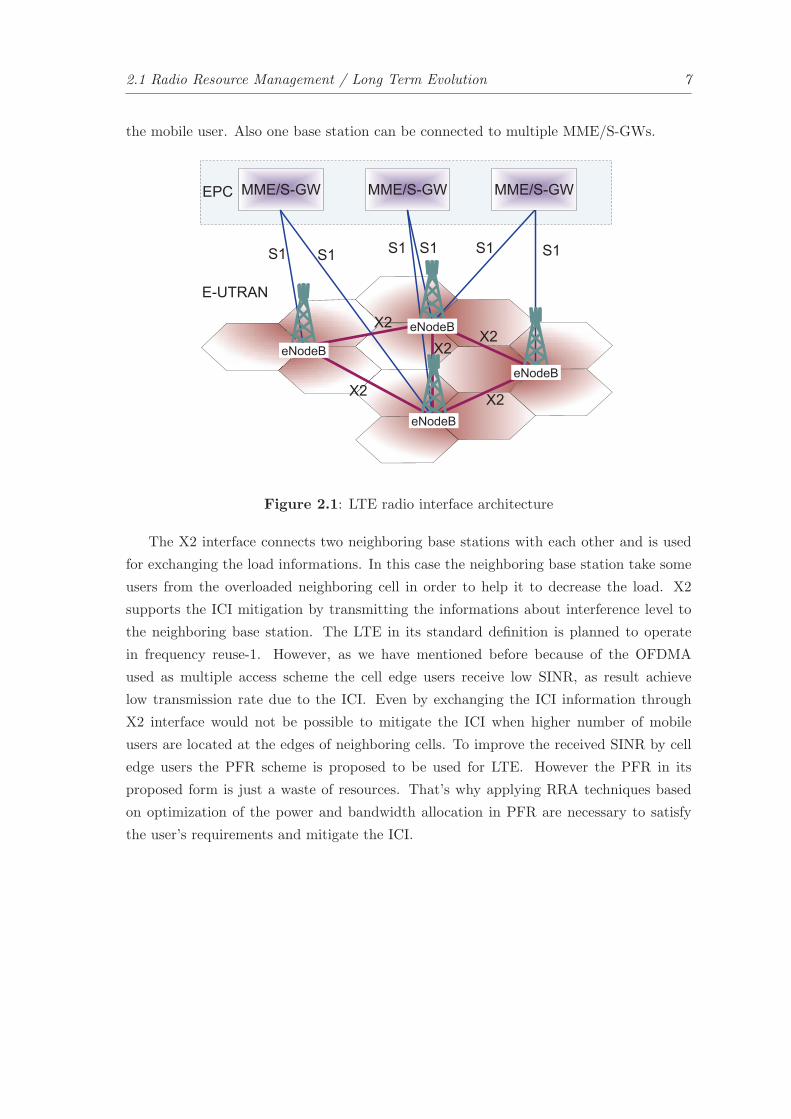
2.1 Radio Resource Management / Long Term Evolution 7
the mobile user. Also one base station can be connected to multiple MME/S-GWs.
X2X2
X2X2
X2
MME/S-GW
S1S1S1 S1 S1 S1
MME/S-GW MME/S-GW
eNodeB
eNodeB
eNodeB
eNodeB
EPC
E-UTRAN
Figure 2.1: LTE radio interface architecture
The X2 interface connects two neighboring base stations with each other and is used
for exchanging the load informations. In this case the neighboring base station take some
users from the overloaded neighboring cell in order to help it to decrease the load. X2
supports the ICI mitigation by transmitting the informations about interference level to
the neighboring base station. The LTE in its standard definition is planned to operate
in frequency reuse-1. However, as we have mentioned before because of the OFDMA
used as multiple access scheme the cell edge users receive low SINR, as result achieve
low transmission rate due to the ICI. Even by exchanging the ICI information through
X2 interface would not be possible to mitigate the ICI when higher number of mobile
users are located at the edges of neighboring cells. To improve the received SINR by cell
edge users the PFR scheme is proposed to be used for LTE. However the PFR in its
proposed form is just a waste of resources. That’s why applying RRA techniques based
on optimization of the power and bandwidth allocation in PFR are necessary to satisfy
the user’s requirements and mitigate the ICI.


3Optimization Techniques for
RRM in Wireless
Communications
FROM the Shanon capacity formula it is well known that requirement for higher trans-
mission rate by communication system depends on the available spectrum and trans-
mit power. The spectrum resources are limited due to very high cost for spectrum license,
as well as power increase is limited due to interference. Furthermore, the number of users
is increasing together with the requirements for higher transmission data rate. So the
question is how we can satisfy the user’s requirements with radio resources that we have
already. The response is using optimization techniques to optimize the spectrum alloca-
tion as well as power allocation. This makes the wireless communication systems more
efficient and capable for satisfying the user’s requirements. There are many optimization
techniques that offers flexible ways to formulate the optimization problems for RRA in
wireless communication. In this chapter we are discussing only two of them since in the
most of our work throughout the thesis we use such techniques to formulate and solve
the optimization problems for RRA. The used techniques are dual decomposition and
geometric programming. In Section 3.1 some of the theories behind DDT is discussed.
For a simple optimization problem in standard form, the formulation of the Lagrangian is
shown. Furthermore, in this section some of the Karush-Kuhn-Tucker (KKT) conditions
for optimality are presented which are quite useful to derive the analytical solutions for
resource allocations. In Section 3.2 the GP for wireless communication is discussed. In this
section the standard form of GP is presented. Another extended form of GP named the
9

10 Chapter 3. Optimization Techniques for RRM in Wireless Communications
maximization of the minimum polynomials that has found many applications in solving
the interference mitigation problems for wireless communication is presented also. At the
end of this chapter the way of converting the Generalized Geometric Programming (GGP)
into GP and their form in Matlab Software for Disciplined Convex Programming (CVX)
is presented also.
3.1 Dual Decomposition Techniques for Wireless Communica-tions
Applying DDT for solving the RRM optimization problems in wireless communication is
efficient and fast. Throughout DDT we decompose the optimization problem into two
problems: the primal problem is the optimization problem formulated and the dual prob-
lem that is the problem defined from the Lagrangian of the primal optimization problem.
By formulating the primal and the dual optimization problems we find distributed solu-
tions that are fundamental for large wireless networks [30] and cross-layer optimization
over different layers of communication [31].
3.1.1 The Lagrangian of an Optimization Problem
Following [32] an optimization problem is any maximization or minimization form of an
objective function followed by some inequality and equality constraints. In general form
a minimization optimization problem is written as follows
minimizex
g0(x) (3.1a)
subject to
gi(x) ≤ 1, i = 1, ..., q (3.1b)
hj(x) = 1, i = 1, ..., q (3.1c)
where g0 : Rn → R is the objective (cost) function, gi : Rn → R are the inequality
function and hj : Rn → R are the equality functions. Any optimization problem of
form (3.1) is said to be convex if the objective (3.1a) and the constraints (3.1b)-(3.1c) are
convex. More details about convex functions can be found in [32].
The Lagrangian for the optimization problem (3.1) is written as follows
L(x,λ,µ) = g0(x) + λT g(x) + µTh(x) (3.2)
where λ is the vector elements of Lagrange multiplier that weights the functions g(x)
defined by gi(x) in the inequalities and µ is the vector elements of Lagrange multiplier
that weights the functions h(x) defined by hj(x) in the equalities.

3.1 Dual Decomposition Techniques for Wireless Communications 11
The Lagrangian is important for solving optimization problems in wireless communi-
cation because during formulation of the optimization problem we won’t wonder if it is
convex or non-convex, since its dual optimization problem is always convex. The dual
Lagrange problem is as follows
maximize G(λ,µ) (3.3a)
subject to
λ ≥ 0 (3.3b)
where G(λ,µ) denotes the dual objective. The Lagrangian and its dual function have found
a large application in solving the network utility and cross-layer optimization problems for
wireless communications networks [31], [33], [30], [34], [35]. Even the primal optimization
problem (3.1) is non-convex the weak duality holds [32] such that optimal solution for the
dual problem (3.3) is smaller or equal to the optimal solution for the primal optimization
problem (3.1).
3.1.2 KKT optimality conditions
To derive analytical equations for optimization problem (3.1) under the assumptions that
all functions in the objective, equalities and inequalities are differentiable even without
knowing about the convexity, we use the KKT conditions [32]. Some of the KKT conditions
that are important for solving convex or concave power allocation problems in Chapter 5
are shown in the following
x � 0, (3.4a)
λT g(x) ≤ 0, (3.4b)
µTh(x) = 0, (3.4c)
λ � 0, (3.4d)
λTx = 0, (3.4e)
∇Lx = 0, (3.4f)
where � denotes the component-wise inequality. The first condition (3.4a) shows the
positivity for optimization variables. The conditions (3.4b) and (3.4c) show the equations
for the inequality and equality functions weighted by respective Lagrange multipliers. The
positivity of Lagrange multiplier λ is defined by Equation (3.4d). The Slater condition
is defined by Equation (3.4e). The last equation (3.4f) defines the first derivative of
Lagrangian with respect to the optimization variable.

12 Chapter 3. Optimization Techniques for RRM in Wireless Communications
3.2 Geometric Programming for Wireless Communications
Geometric programming is nonlinear and non-convex optimization technique that is widely
used in solving RRA problems in wireless networks. Even though GPs are non-convex,
there are existing methods to convert them into forms, which are suitable to finding
solution. In the high-SINR regime [14] the problems of maximizing the sum-rate can be
converted into GP and solved efficiently. However in most of the wireless communication
technologies, the interference is the limiting factor for the performance of them. So the
GP offers flexibility in formulation the RRA problems that mitigate the interference and
improve the throughput, minimize the transmission energy, minimize the delay etc.
3.2.1 Geometric Programming in Basic Form
The GP in its basic form [36], [37] is a constrained optimization problem formulated by
the objective and inequality or equality or both constraints. The objective in general is a
posynomial or a monomial. However, every monomial is also a posynomial. The equalities
can be also posynomials expect monomials, while the equalities can be only monomials.
The GP in its basic form is given as follows
minimizex
g0(x) (3.5a)
subject to
gi(x) ≤ 1, i = 1, ..., q (3.5b)
hj(x) = 1, i = 1, ..., q (3.5c)
where the posynomials gi(x) in the objective (3.5a) or in the inequality constraints (3.5b)
are defined in the following form
g(x) =K∑
k=1
wkxδ1k1 xδ2k2 ...x
δqkq (3.6)
such that w > 0 and δqk ∈ R. The monomials in the objective (3.5a) or any of the
constraints (3.5b)-(3.5c) are defined in the following form
g(x) = wxδ11 xδ22 ...xδqq . (3.7)
For example: πx0.71 + x101 x32x−23 is a posynomial and x−10
1 x32x−23 x4 is a monomial.
The RRA problems in wireless communication is not trivial to be formulated directly
into GP forms as given by Equation (3.5). However for specific extended forms of GPs
exist different methods of transforming them into GP. In the next section we explain one
of the extended forms of GPs called GGP, which under a simple transformation becomes
GP. After such forms are converted into GP form like in Equation (3.5), their solution be
found easily by interior-point methods [38] or matlab based tool called CVX [39].

3.2 Geometric Programming for Wireless Communications 13
Maximum of Minimum Posynomials
For the RRA problems in wireless communication one of the most GGP form used is
the maximization of the minimum posynomials. So in this subsection we are explaining
this form taking a simple example. A simple example is the maximization of the two
posynomials that in GGP form is written as in the following
maximizex
min{g1(x), g2(x)} (3.8a)
subject to
g3(x) ≤ 1, (3.8b)
h1(x) = 1 (3.8c)
Such optimization problems are in use by UMTS for load balancing. Similar to UMTS also
in LTE the maximization of the minimum SINR and the maximization of the minimum
rate belongs to the maximization of the minimum posynomials.
3.2.2 Transformation of the GGP to GP and its form in CVX
As we mentioned earlier the optimization problems similar to the one given by Equa-
tion (3.8) can not be solved directly. However, there are methods explained in [32], [36]
and [37] where under the log transformation of the variables such problems can be con-
verted into convex GP ones. In the following we show how the optimization problem given
by Equation (3.8) can be transformed into GP. So we introduce an auxiliary variable z
that lower bounds the functions in the objective (3.8a) and places them as constraints.
The optimization problem (3.8) in GP form becomes
minimizex,z
1
z(3.9a)
subject to
g1(x) ≥ z, (3.9b)
g2(x) ≥ z, (3.9c)
g3(x) ≤ 1, (3.9d)
h1(x) = 1 (3.9e)
The GP optimization problem given by Equation (3.9) in CVX will have the following
structure
cvx begin gp
variables x, z
minimize 1/z
subject to g1(x) ≥ z
g2(x) ≥ z
14 Chapter 3. Optimization Techniques for RRM in Wireless Communications
g3(x) ≤ 1
h1(x) = 1
cvx end
4
Capacity Density
Maximization for LTE
THE high interference at the cell edge for mobile communication systems that use the
OFDMA is an issue that should be mitigated. To mitigate the ICI many frequency
re-use schemes have been proposed. One of the promising scheme is the PFR, which is a
combination of frequency reuse-1 and the frequency reuse-3 such that frequency reuse-1 is
assigned for cell center users and frequency reuse-3 is assigned for cell edge users. In this
chapter, I show the results on how the cell edge bandwidth is re-used for the cell center
users in order to improve the cell capacity density assuming that cell edge users are idle.
In Section 4.1 the geometry of the cell cluster model is shown with all its parameters that
characterize the user’s channel and the received power and interference. To calculate the
average received SINR for a user located at the cell center or at the cell edge, we used
the geometry of the cell cluster model and path-loss model. In Section 4.2, is shown the
bandwidth re-allocation scheme for PFR that represents the frequency bands allocation
per sub-carrier basis and per frequency band basis. In Section 4.3, are presented the
mathematical derivations for cell capacity density. To make such derivations the cell cluster
model and frequency reuse pattern are taken into account. Furthermore, in this section
the optimization problem for maximizing the cell capacity density under the bandwidth
re-allocation scheme is formulated. At the end of this chapter simulation results are drawn
to illustrate the gain in capacity density when cell edge bandwidth is re-allocated to the
inner users.
15

16 Chapter 4. Capacity Density Maximization for LTE
4.1 Geometry of Cell Cluster Model
To calculate the cell capacity density the basic principle is to design a cell cluster model.
In the following a cell cluster model similar to the model in [6] is shown, which contains a
base station BS0 in the center of the cluster and six neighboring base stations BSk, with
k = 1, . . . 6,. Each base station is considered to offer coverage over a regular hexagon area.
The cluster model is shown in Figure 4.1.
X
BS0
BS1
BS6
BS5
BS4
BS3
BS2
r
X
YU
R
)( !
BS1
Y
X
r1
r2
r3
r4
r5
r6
r
R
U
Y
d BS0
Figure 4.1: Cell cluster with radius classification criteria
In the cell cluster shown in Figure 4.1, each base station is equipped with three sector-
ized antennas, where each antenna radiates over an angle 1200. As it is shown in Figure
4.1 the user U that is located at cartesian coordinates (X,Y ) is far from the serving base
station for a distance r. The SINR received by user U is given by the following equation
SINR =Pr
Pintra−cell + Pinter−cell +N0, (4.1)
where Pr is the received power, Pintra−cell is the interference that comes from the users
within the same cell and Pinter−cell is the interference that comes from the users located
in the neighboring cells. The noise spectral density is denoted by N0. Since LTE use
OFDMA as multiple access scheme in the downlink [40], there is no intra-cell interference.
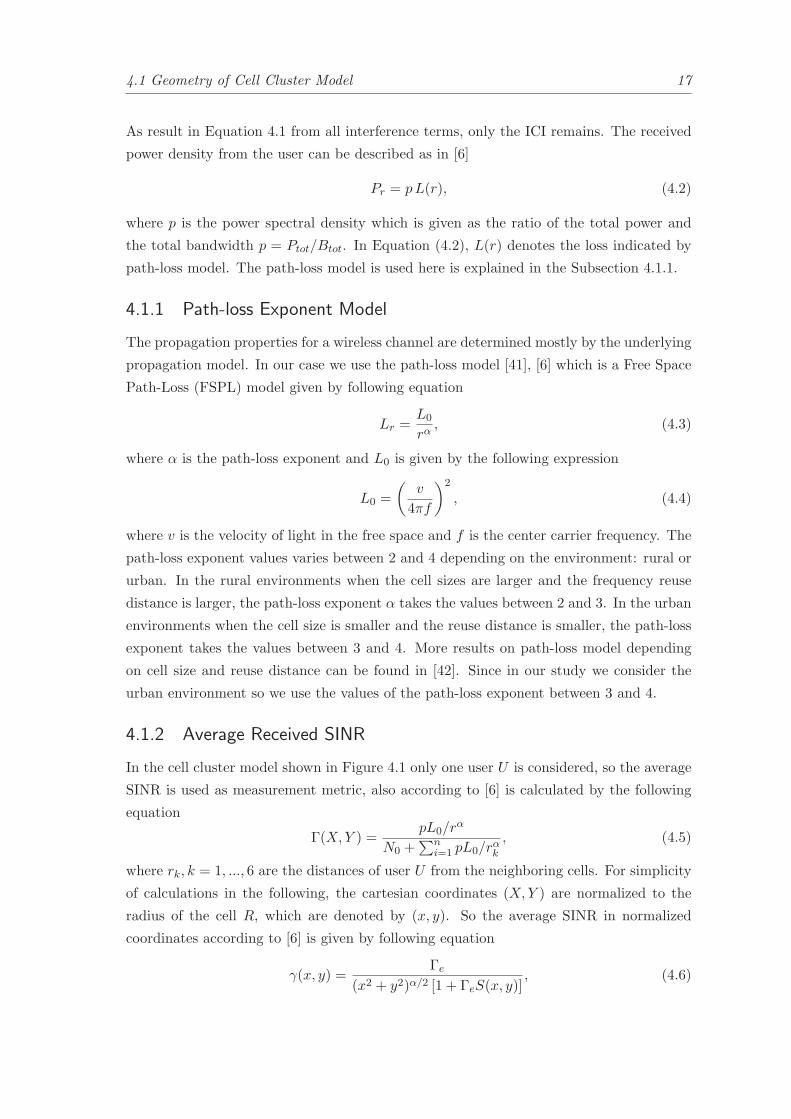
4.1 Geometry of Cell Cluster Model 17
As result in Equation 4.1 from all interference terms, only the ICI remains. The received
power density from the user can be described as in [6]
Pr = pL(r), (4.2)
where p is the power spectral density which is given as the ratio of the total power and
the total bandwidth p = Ptot/Btot. In Equation (4.2), L(r) denotes the loss indicated by
path-loss model. The path-loss model is used here is explained in the Subsection 4.1.1.
4.1.1 Path-loss Exponent Model
The propagation properties for a wireless channel are determined mostly by the underlying
propagation model. In our case we use the path-loss model [41], [6] which is a Free Space
Path-Loss (FSPL) model given by following equation
Lr =L0
rα, (4.3)
where α is the path-loss exponent and L0 is given by the following expression
L0 =
(
v
4πf
)2
, (4.4)
where v is the velocity of light in the free space and f is the center carrier frequency. The
path-loss exponent values varies between 2 and 4 depending on the environment: rural or
urban. In the rural environments when the cell sizes are larger and the frequency reuse
distance is larger, the path-loss exponent α takes the values between 2 and 3. In the urban
environments when the cell size is smaller and the reuse distance is smaller, the path-loss
exponent takes the values between 3 and 4. More results on path-loss model depending
on cell size and reuse distance can be found in [42]. Since in our study we consider the
urban environment so we use the values of the path-loss exponent between 3 and 4.
4.1.2 Average Received SINR
In the cell cluster model shown in Figure 4.1 only one user U is considered, so the average
SINR is used as measurement metric, also according to [6] is calculated by the following
equation
Γ(X,Y ) =pL0/r
α
N0 +∑n
i=1 pL0/rαk, (4.5)
where rk, k = 1, ..., 6 are the distances of user U from the neighboring cells. For simplicity
of calculations in the following, the cartesian coordinates (X,Y ) are normalized to the
radius of the cell R, which are denoted by (x, y). So the average SINR in normalized
coordinates according to [6] is given by following equation
γ(x, y) =Γe
(x2 + y2)α/2 [1 + ΓeS(x, y)], (4.6)
18 Chapter 4. Capacity Density Maximization for LTE
where Γe is the edge Signal-to-Noise-ratio (SNR) and is defined by
Γe =pL
N0Rα. (4.7)
The sum of all path-loss distances rk is denoted by S(x, y) and given by following equation
S(x, y) =n∑
k=1
[
(x− xk)2 + (y − yk)
2]−α/2
, (4.8)
where the normalized coordinates for the first tier of the interferer base stations are cal-
culated using equations
xk =√3 cos(k − 1)
π
3, 1 ≤ k ≤ 6, (4.9)
yk =√3 sin(k − 1)
π
3, 1 ≤ k ≤ 6. (4.10)
Similarly to the equations for normalized coordinates of the first tier of interferer base
stations, we define the equations for the normalized coordinates of the second tier interferer
base stations as follows
xk = 2√3 cos(k − 1)
π
3, 7 ≤ k ≤ 18, (4.11)
yk = 2√3 sin(k − 1)
π
3, 7 ≤ k ≤ 18. (4.12)
The ICI is usually critical for cell edge users because the neighboring cells may use the same
sub-carriers in a single frequency reuse-1 network. Also the users in the center of the cell
use the same carriers, but they are more isolated from ICI because of the macro-scale path-
loss. In order to minimize the ICI, a common approach is to split the cells into two regions:
in a so-called FR-region and a PR-region. The FR-region is located around the base
station, while the PR-region is located at the cell edge. All three sectors in FR-region use
the same frequency bands like in reuse-1. In PR-region the three neighboring sectors use
different frequency bands. Implying this frequency planning for the PR frequency bands,
the PR-region can be considered ICI-free because the frequencies which are allocated for
users in this region are different from the frequencies which are allocated to the users in
neighboring cells. The classification for a user in cell is determined based on its received
SINR. Depending on the value for the threshold on received SINR, we classify the users
to the corresponding cell regions. If the received SINR from a user is higher than SINR
threshold, that user is classified as inner user otherwise as outer user. After classifying the
user, the scheduler decides which Physical Resource Block (PRB) to allocate to the user.
One PRB contains 12 subcarriers where each subcarrier is 15 kHz in frequency domain [43].
The boundary between these two regions in polar coordinates is denoted as β(θ), with θ
specifying the azimuth angle. Furthermore, under the assumption of a circular boundary

4.2 Frequency Reuse Schemes 19
ρ = β(θ) between the cell center region and the cell edge region, the average SINR for
those regions in polar coordinates is formulated as follows
γρ(r) =
{
Γe
rα[1+ΓeS(r)], 0 < r ≤ ρ,
Γe
rα , ρ < r ≤ 1.(4.13)
4.2 Frequency Reuse Schemes
An exemplary frequency reuse pattern model for bandwidth allocation in PFR is presented
in Figure 4.2.
BS1BS1
BS2
BS3
BS6
BS2
BS4
BS5
BS1
12
13
14
Figure 4.2: Frequency reuse pattern and bandwidth partitioning
In the frequency reuse pattern shown in Figure 4.2 the sectors are denoted by S12, S13
and S14 where the first subscript denotes the FR-band and the second subscript denotes
the PR-bands. The equation for the total bandwidth used, compliant to the model shown
in Figure 4.2 is given by following equation
Btot = BFR + 3BPR, (4.14)

20 Chapter 4. Capacity Density Maximization for LTE
where BFR denotes the bandwidth allocated in FR-region and BPR denotes the bandwidth
allocated in PR-region. A fixed bandwidth allocation scheme is assumed here with ratio
between bandwidths as BFR/BPR = 3.
Let us now assume all cells to be populated homogeneously with users over their
area and in average all cells utilize the same transmit power. As result all subcarriers
in all regions for the cells in PFR experience the same transmit power in downlink. The
bandwidth allocation per subcarrier where all sucarriers have the same transmit power in
the downlink as it is shown in Figure 4.3.
...
... ...
...
...
...
12
13
14
Figure 4.3: Downlink subcarrier allocation
In practical systems over the area of cells the users are not distributed uniformly, which
means that more users can be concentrated in the area of FR-region (near the base station)
than in the area of PR-region. In such case we say that cell is not loaded homogeneously
over its area. To decrease the cell load in the FR region, it is necessary to re-allocate
the bandwidth from PR-region to the FR-region. In make such re-allocation we introduce
the parameter t which splits the PR-bandwidth in two parts. The way of allocating
the bandwidth from PR-region in FR-region is shown by the bandwidth re-allocation
scheme presented in Figure 4.4. The bandwidth which is re-allocated from the PR-region
to the FR-region is considered to be ICI-free due to the assumption made earlier for
4.3 Capacity density for Partial Frequency Reuse 21
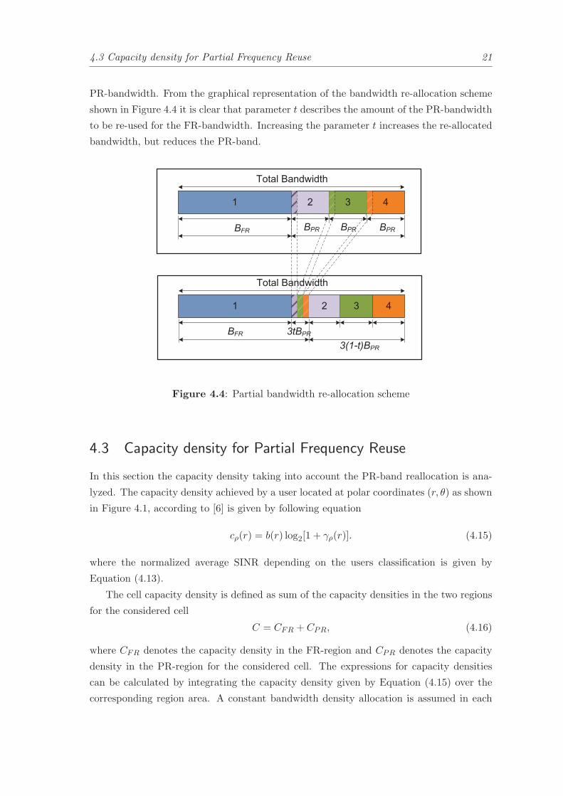
PR-bandwidth. From the graphical representation of the bandwidth re-allocation scheme
shown in Figure 4.4 it is clear that parameter t describes the amount of the PR-bandwidth
to be re-used for the FR-bandwidth. Increasing the parameter t increases the re-allocated
bandwidth, but reduces the PR-band.
Total Bandwidth
432
BFR BPR
Total Bandwidth
4321
1
BPRBPR
BFR 3tBPR
3(1-t)BPR
Figure 4.4: Partial bandwidth re-allocation scheme
4.3 Capacity density for Partial Frequency Reuse
In this section the capacity density taking into account the PR-band reallocation is ana-
lyzed. The capacity density achieved by a user located at polar coordinates (r, θ) as shown
in Figure 4.1, according to [6] is given by following equation
cρ(r) = b(r) log2[1 + γρ(r)]. (4.15)
where the normalized average SINR depending on the users classification is given by
Equation (4.13).
The cell capacity density is defined as sum of the capacity densities in the two regions
for the considered cell
C = CFR + CPR, (4.16)
where CFR denotes the capacity density in the FR-region and CPR denotes the capacity
density in the PR-region for the considered cell. The expressions for capacity densities
can be calculated by integrating the capacity density given by Equation (4.15) over the
corresponding region area. A constant bandwidth density allocation is assumed in each

22 Chapter 4. Capacity Density Maximization for LTE
region such that for given ρ, the b(r) becomes BFR in the FR-region and BPR in the
PR-region. So the expressions for CFR becomes
CFR = 2π
∫ ρ
0BFR log2
(
1 +Γe
rα [1 + ΓeS(r)]
)
rdr, (4.17)
and the expression for and CPR
CPR = 2π
∫ 1
ρBPR log2
(
1 +Γe
rα
)
rdr. (4.18)
To account for the PR-bandwidth re-allocation to the FR-region, we go through three
steps. In the first, step we include the parameter t in Equation (4.18) and split it into two
parts as shown by following equation
CPR = 2π
∫ 1
ρtBPR log2
(
1 +Γe
rα
)
rdr
+ 2π
∫ 1
ρ(1− t)BPR log2
(
1 +Γe
rα
)
rdr. (4.19)
In the second step, we replace the lower bound ρ by 0 and the upper bound 1 by
ρ in the first integral of Equation (4.19). Now the modified expression for capacity in
PR-region becomes
CPR(t) = 2π
∫ ρ
0tBPR log2
(
1 +Γe
rα
)
rdr
+ 2π
∫ 1
ρ(1− t)BPR log2
(
1 +Γe
rα
)
rdr. (4.20)
Looking Equation (4.20) it is clear that the first integral accounts for capacity density of
FR-region. And in the final step, we place the Equation (4.17) and Equation (4.20) into
Equation (4.16) to formi the expression for cell capacity density that takes into account
the PR-bandwidth re-allocation. The equations for cell capacity density is formulated as
in the following
C(t, ρ) = 2π
∫ ρ
0BFR log2
(
1 +Γe
rα [1 + ΓeS(r)]
)
rdr
+ 2π
∫ ρ
0tBPR log2
(
1 +Γe
rα
)
rdr
+ 2π
∫ 1
ρ(1− t)BPR log2
(
1 +Γe
rα
)
rdr. (4.21)
By increasing the parameter t we re-allocate more bandwidth from PR-region in FR-
region. To maximize the cell capacity density constrained by frequency partitioning ρ and
4.3 Capacity density for Partial Frequency Reuse 23
bandwidth re-allocation t we formulate the following optimization problem
maximizeρ,t
C (4.22a)
subject to
0 ≤ ρ ≤ 1 (4.22b)
0 ≤ t ≤ 1. (4.22c)
Numerical Simulations: Capacity density and frequency partitioning radius
In this section, the simulation results for capacity density and frequency partitioning
radius taking into account the PR-bandwidth re-allocation are shown. The simulation
parameters used for simulations are shown in Table 4.1.
Table 4.1: Simulation parameters
parameters value
Total bandwidth Btot 20MHz
Total power Ptot 1W
Noise spectral density N0 −174 dBm/Hz
Center frequency f 2GHz
Path-loss exponent α 3.6
Cell radius R 100m
To get the simulation results for the cell capacity density we use the simulation pa-
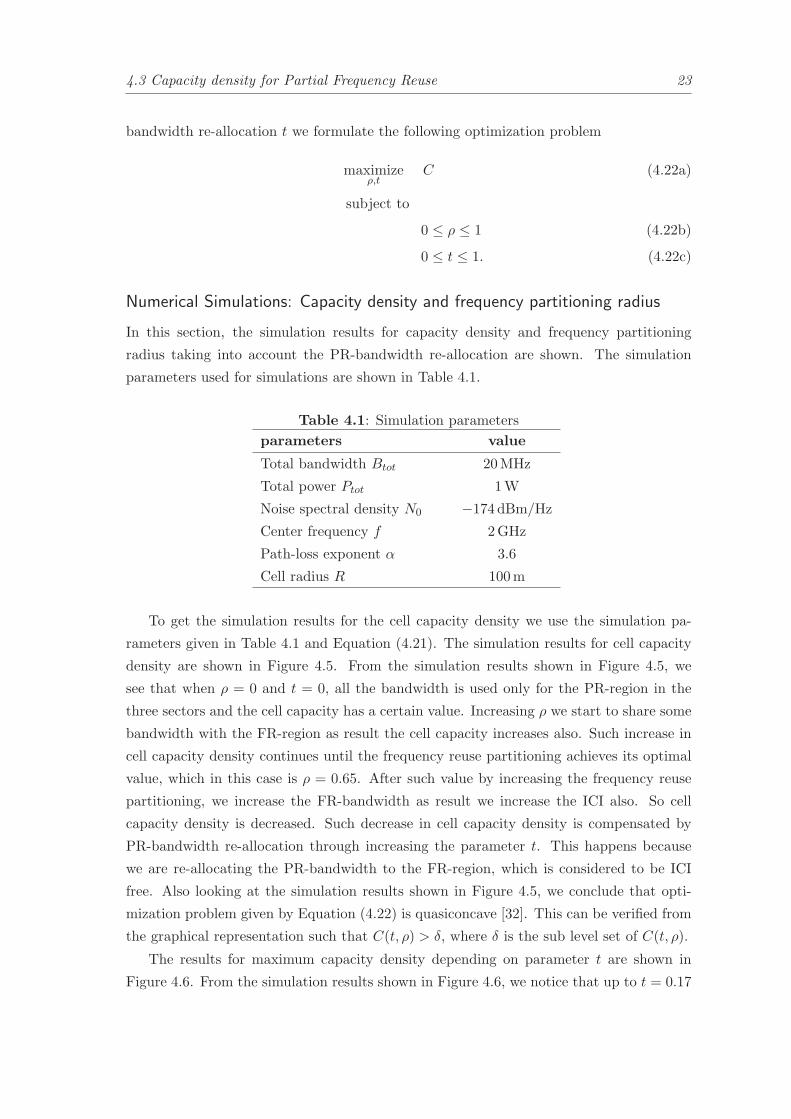
rameters given in Table 4.1 and Equation (4.21). The simulation results for cell capacity
density are shown in Figure 4.5. From the simulation results shown in Figure 4.5, we
see that when ρ = 0 and t = 0, all the bandwidth is used only for the PR-region in the
three sectors and the cell capacity has a certain value. Increasing ρ we start to share some
bandwidth with the FR-region as result the cell capacity increases also. Such increase in
cell capacity density continues until the frequency reuse partitioning achieves its optimal
value, which in this case is ρ = 0.65. After such value by increasing the frequency reuse
partitioning, we increase the FR-bandwidth as result we increase the ICI also. So cell
capacity density is decreased. Such decrease in cell capacity density is compensated by
PR-bandwidth re-allocation through increasing the parameter t. This happens because
we are re-allocating the PR-bandwidth to the FR-region, which is considered to be ICI
free. Also looking at the simulation results shown in Figure 4.5, we conclude that opti-
mization problem given by Equation (4.22) is quasiconcave [32]. This can be verified from
the graphical representation such that C(t, ρ) > δ, where δ is the sub level set of C(t, ρ).
The results for maximum capacity density depending on parameter t are shown in
Figure 4.6. From the simulation results shown in Figure 4.6, we notice that up to t = 0.17
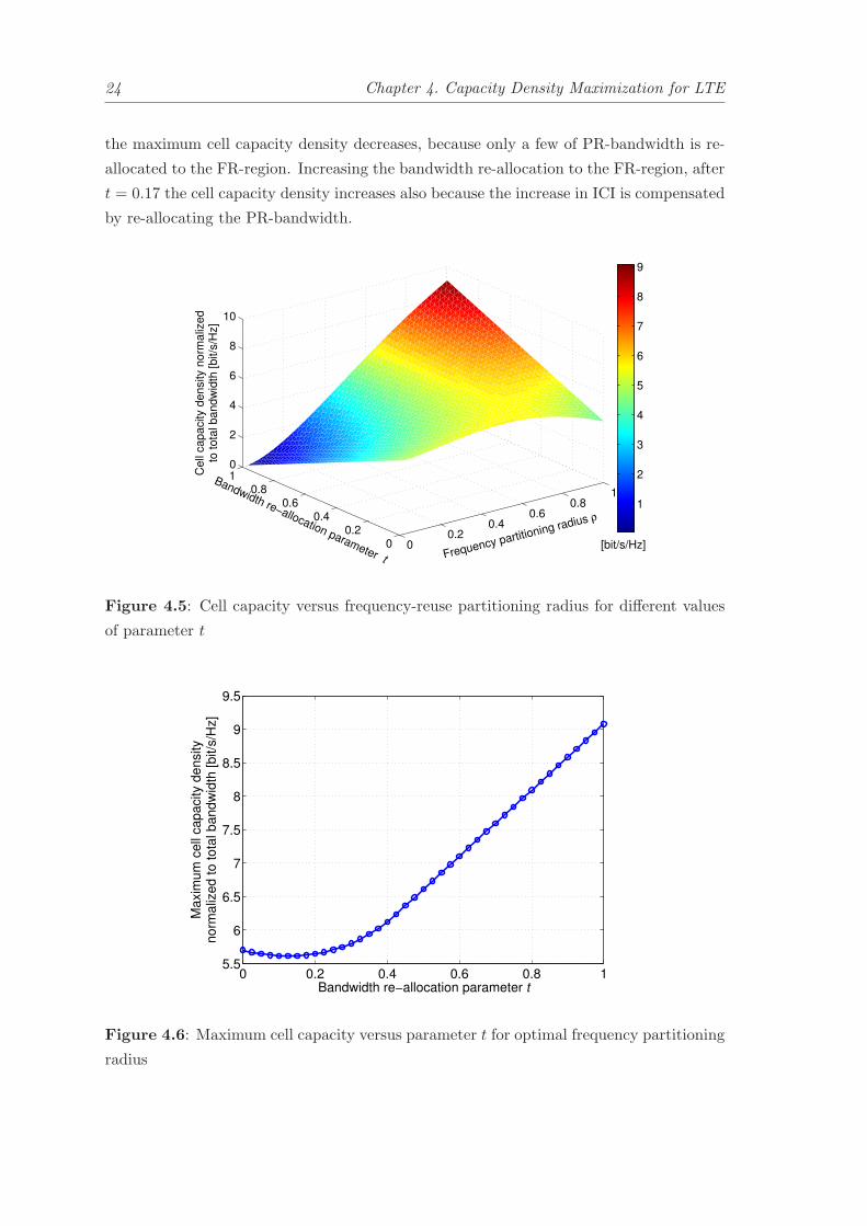
24 Chapter 4. Capacity Density Maximization for LTE
the maximum cell capacity density decreases, because only a few of PR-bandwidth is re-
allocated to the FR-region. Increasing the bandwidth re-allocation to the FR-region, after
t = 0.17 the cell capacity density increases also because the increase in ICI is compensated
by re-allocating the PR-bandwidth.
00.2
0.40.6
0.81
00.2
0.40.6
0.810
2
4
6
8
10
Frequency partitioning radius ρ
Bandwidth re−allocation parameter t
Ce
ll ca
pa
city d
en
sity n
orm
aliz
ed
to t
ota
l b
an
dw
idth
[b
it/s
/Hz]
1
2
3
4
5
6
7
8
9
[bit/s/Hz]
Figure 4.5: Cell capacity versus frequency-reuse partitioning radius for different values
of parameter t
0 0.2 0.4 0.6 0.8 15.5
6
6.5
7
7.5
8
8.5
9
9.5
Bandwidth re−allocation parameter t
Maxim
um
cell
capacity d
ensity
norm
aliz
ed to tota
l bandw
idth
[bit/s
/Hz]
Figure 4.6: Maximum cell capacity versus parameter t for optimal frequency partitioning
radius
5
Power Allocation in Partial
Frequency Reuse
IN this chapter, I show the sum-rate maximization by power allocation. Under the
assumption for uniform power allocation to the inner (cell center) users and to the
outer (cell edge) users, we transform the non-convex optimization problem for sum-rate
maximization into a convex optimization problem.
In Section 5.1, the geometries of two cell cluster models for users classification are
introduced. One is based on the distance threshold, where the users are classified in the
cell regions based on their distance to the serving base station. The second cell cluster
model uses the LSPLA threshold for users classification in the cell regions. To characterize
the time variant properties of the wireless channel the LSPLA with its parameters including
path-loss exponent, antenna gain, penetration loss, small-scale fading and shadowing is
explained in Section 5.2. In Section 5.3, we show the frequency reuse pattern for variable
power and fixed bandwidth allocation, that is applicable with both cell cluster models.
Furthermore, in this section, based on the frequency reuse pattern for PFR, we formulated
the optimization problems which are solvable in a water-filling like power allocation. Even
more to show the importance of the optimal power allocation algorithm in reducing the
ICI and increasing the sum-rate, the simulation are carried out. At the end of this chapter
we show the methods to convert non-convex optimization problems of maximizing the
minimum rate and the sum-power minimization for PFR into convex ones without making
any assumption on power allocation or high-SINR approximation.
25
26 Chapter 5. Power Allocation in PFR
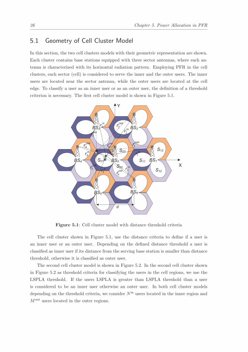
5.1 Geometry of Cell Cluster Model
In this section, the two cell clusters models with their geometric representation are shown.
Each cluster contains base stations equipped with three sector antennas, where each an-
tenna is characterized with its horizontal radiation pattern. Employing PFR in the cell
clusters, each sector (cell) is considered to serve the inner and the outer users. The inner
users are located near the sector antenna, while the outer users are located at the cell
edge. To classify a user as an inner user or as an outer user, the definition of a threshold
criterion is necessary. The first cell cluster model is shown in Figure 5.1.
BS5
BS0
BS2BS3
BS4
BS6
BS1
X
Y
in
1r
in
2r
in
3r
in
4r
in
5r
in
6r
in
0r
out
0r
out
4r
out
3r
out
2r
out
5r
out
6r
out
1r
S11
S12
S13
S01
S02
S03
d
Figure 5.1: Cell cluster model with distance threshold criteria
The cell cluster shown in Figure 5.1, use the distance criteria to define if a user is
an inner user or an outer user. Depending on the defined distance threshold a user is
classified as inner user if its distance from the serving base station is smaller than distance
threshold, otherwise it is classified as outer user.
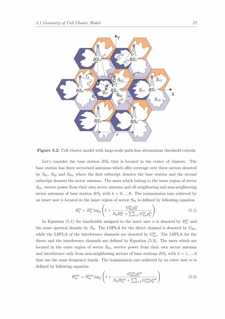
The second cell cluster model is shown in Figure 5.2. In the second cell cluster shown
in Figure 5.2 as threshold criteria for classifying the users in the cell regions, we use the
LSPLA threshold. If the users LSPLA is greater than LSPLA threshold than a user
is considered to be an inner user otherwise an outer user. In both cell cluster models
depending on the threshold criteria, we consider N in users located in the inner region and
Mout users located in the outer regions.
5.1 Geometry of Cell Cluster Model 27
BS0X
Y
S02
S03
d
out
6r
in
6r
S01
in
5r
out
4r
in
4r
out
5r
BS4
BS5
BS0
BS6
S12
S11
in
1r
S13
BS1
out
1r
out
2r
in
2rout
3r
out
0r
in
3r
BS2BS3
S02
S03in
0r
Figure 5.2: Cell cluster model with large-scale path-loss attenuation threshold criteria
Let’s consider the base station BS0 that is located in the center of clusters. The
base station has three sectorized antennas which offer coverage over three sectors denoted
by S01, S02 and S03, where the first subscript denotes the base station and the second
subscript denotes the sector antenna. The users which belong to the inner region of sector
S01, receive power from their own sector antenna and all neighboring and non-neighboring
sector antennas of base station BSk with k = 0, ..., 6. The transmission rate achieved by
an inner user n located in the inner region of sector S01 is defined by following equation
Rinn = Bin
n log2
(
1 +Gin
0npin0
N0Binn +
∑6k=1G
inknp
ink
)
. (5.1)
In Equation (5.1) the bandwidth assigned to the inner user n is denoted by Binn and
the noise spectral density by N0. The LSPLA for the direct channel is denoted by G0n,
while the LSPLA of the interference channels are denoted by Ginkn. The LSPLA for the
direct and the interference channels are defined by Equation (5.3). The users which are
located in the outer region of sector S01, receive power from their own sector antenna
and interference only from non-neighboring sectors of base stations BSk with k = 1, ..., 6
that use the same frequency bands. The transmission rate achieved by an outer user m is
defined by following equation
Routm = Bout
m log2
(
1 +Gout
0mpout0
N0Boutm +
∑6k=1G
outkmpoutk
)
(5.2)
28 Chapter 5. Power Allocation in PFR
The bandwidth allocated to the outer user m is denoted by Boutm . The LSPLA for the
direct channel to the outer user m is denoted by Gout0m , while the interference channels to
the outer user m are denoted by Goutkm. The direct and the interference channels similarly
to the inner user, are defined by Equation (5.3). The position of the users within the cell
is determined by their polar coordinates (r, θ) converted from the cartesian coordinates
(x, y). More distant base stations are not considered in the cluster models shown in
Figure 5.1 and Figure 5.2, due to increased complexity, however all the results can be
extended to consider more distant base station as well.
5.2 Large-scale Path-loss Attenuation
The wireless channel is time variant not only because of the movement of the Receiver (Rx),
but also because of the movement of the surrounding objects. Even when a mobile is
not moving, due to the movement of the surrounding objects the signal can experience
small-scale fading [44]. To consider most of the effects which determine the time variant
properties of the wireless channels, in the following an extended version of LSPLA [45] is
analyzed. The LSPLA of a direct channel or an interference channel including antenna
gain, penetration loss, log-normal shadowing and small-scale fading (fast fading) is defined
by following equation
Gski = − [128.1 + 10α log10(rk/1000m)−Ak + Lp +Xσ + F ] . (5.3)
The Gski is in dB, the superscript s ∈ {in, out} denotes the inner or the outer users, the
subscript i ∈ {n,m} denotes the users index. The number 128.1 used in Equation (5.3)
depends on the center frequency, where for the frequency 2GHz that number is recom-
mended by 3GPP standardization [46]. The path-loss exponent similar for the path-loss
exponent model is denoted by α, the distance between the mobile station and the base
station is denoted by r in m, the sum of the mobile antenna gain and the base station
antenna gain is denoted by Ak in dBi, the penetration loss by Lp in dB, the log-normal
shadowing by Xσ in dB. The small-scale fading denoted by F is in dB.
5.2.1 Antenna Gain
In our cell cluster models, we use hexagonal cells where each hexagonal area is served by
signals transmitted from directive antennas. The directive antenna is characterized by its
gain, which depends on the antenna radiation pattern. We consider the horizontal antenna
gain [46], [47] defined by the horizontal antenna pattern given by following equation
A(θ) = −min
[
12
(
θ
θ3dB
)2
, Am
]
(5.4)
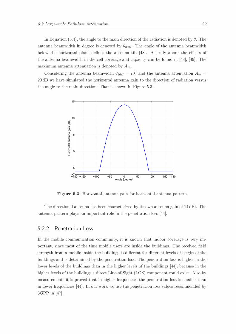
5.2 Large-scale Path-loss Attenuation 29
In Equation (5.4), the angle to the main direction of the radiation is denoted by θ. The
antenna beamwidth in degree is denoted by θ3dB. The angle of the antenna beamwidth
below the horizontal plane defines the antenna tilt [48]. A study about the effects of
the antenna beamwidth in the cell coverage and capacity can be found in [48], [49]. The
maximum antenna attenuation is denoted by Am.
Considering the antenna beamwidth θ3dB = 700 and the antenna attenuation Am =
20dB we have simulated the horizontal antenna gain to the direction of radiation versus
the angle to the main direction. That is shown in Figure 5.3.
−180 −150 −100 −50 0 50 100 150 180−7
−5
0
5
10
15
Angle [degree]
Ho
rizon
tal a
nte
nn
a g
ain
[d
Bi]
Figure 5.3: Horizontal antenna gain for horizontal antenna pattern
The directional antenna has been characterized by its own antenna gain of 14 dBi. The
antenna pattern plays an important role in the penetration loss [44].
5.2.2 Penetration Loss
In the mobile communication community, it is known that indoor coverage is very im-
portant, since most of the time mobile users are inside the buildings. The received field
strength from a mobile inside the buildings is different for different levels of height of the
buildings and is determined by the penetration loss. The penetration loss is higher in the
lower levels of the buildings than in the higher levels of the buildings [44], because in the
higher levels of the buildings a direct Line-of-Sight (LOS) component could exist. Also by
measurements it is proved that in higher frequencies the penetration loss is smaller than
in lower frequencies [44]. In our work we use the penetration loss values recommended by
3GPP in [47].

30 Chapter 5. Power Allocation in PFR
5.2.3 Shadowing
The communication between mobile and base station is realized through the wireless
channel which is sometimes LOS, but in most of the cases is Non-Line-of-Sight (NLOS),
with many paths generated by reflection from the objects, diffraction etc. Sometimes
the mobile station is near the base station, but because of the movement of the mobile
station behind a building or a hill, the received signal is decreased. The effect of decrease
in the received signal amplitude for a mobile station because the mobile is in shadow of
the transmitted paths from the base station is called shadowing [50]. The shadowing is
characterized by a log-normal distribution [51] defined by Xσ ∼ N (0, σ)
5.2.4 Small-scale Fading
As result of reflections, multiple signals arrive from Transmitter (Tx) to Rx with different
phases and amplitudes such that at Rx those signals are combined. Combining the signals
at Rx, could increase the interference which results in change of amplitude for the received
signal. Such effect is called small-scale fading.
At the operating frequency of LTE, even a small movement by 10 cm for the mobile
station could have a positive or a negative effect on the received signal amplitude of the
mobile station, due to small-scale fading [50]. In our study we consider the small-scale
fading as chi-square distribution χ22 with two degrees of freedom. The small-scale fading
contributes in LSPLA given by Equation (5.3) only for the directed channels. The effect
of the small-scale fading for the interference channels is neglected. This is because some
components increase the amplitude of interference signal and some of the components
decrease that amplitude, so when they combine at the receiver the effect is almost zero [51].
5.3 Variable Power and Fixed Bandwidth Allocation Scheme
In this section, we show the power allocation for fixed bandwidth allocation scheme in
PFR. The bandwidth allocation is considered to be fixed in all regions of the cells, while
the power allocation is considered to be variable such that it is optimized. The bandwidth
and power allocation scheme is shown in Figure 5.4.
From the graphical representation in Figure 5.4 it is shown that half of the maximum
cell bandwidth is allocated in the inner regions like in reuse-1, and the other half of the
bandwidth is slitted in three equal parts like in reuse-3 and allocated in neighboring cell
edge regions. By splitting the total bandwidth as the inner bandwidth and the outer
bandwidth as we mentioned before, we minimize the ICI at the cell edge, where more
power allocation is necessary due to the distance of the outer users from their own base
station. For the fixed bandwidth and variable power allocation scheme shown in Figure 5.4

5.4 Power Allocation Algorithm 31
we show the power allocation algorithm in the following.
inp
outp
inB
outB
maxB
Frequency
maxP
inp
outp
inB out
B Frequency
maxP
inp
outp
inB
outB Frequency
Powermax
P
Sector 1
Sector 3
Sector 2
Figure 5.4: Frequency reuse pattern for fixed bandwidth allocation
5.4 Power Allocation Algorithm
In this section, we present the power allocation algorithm that classifies the users in the
cell regions based on the distance threshold criteria. The power allocation algorithm is
presented by Algorithm 1.
Algorithm 1 Power Allocation Algorithm
Require: rtgt, (r, θ)
1: if r < rtgt then
2: (rin, θin)← (r, θ)
3: else
4: (rin, θin)← (r, θ)
5: end if
6: Calculate the values of:
pin0 , pink , p
out0 , poutk ,
using power allocation given by Equation (5.5).
The Algorithm 1, during classification saves the positions of the inner users at polar
coordinates (rin, θin) and the outer users at polar coordinates (rout, θout). At the last step
it applies the power allocation problem to optimally allocate the power in the cell regions.
32 Chapter 5. Power Allocation in PFR
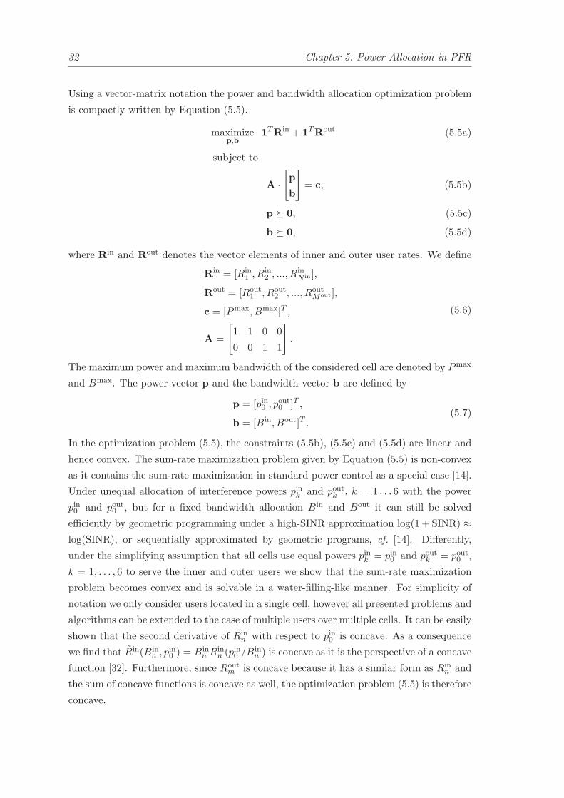
Using a vector-matrix notation the power and bandwidth allocation optimization problem
is compactly written by Equation (5.5).
maximizep,b
1TRin + 1TRout (5.5a)
subject to
A ·[
p
b
]
= c, (5.5b)
p � 0, (5.5c)
b � 0, (5.5d)
where Rin and Rout denotes the vector elements of inner and outer user rates. We define
Rin = [Rin1 , R
in2 , ..., R
inN in ],
Rout = [Rout1 , Rout
2 , ..., RoutMout ],
c = [Pmax, Bmax]T ,
A =
[
1 1 0 0
0 0 1 1
]
.
(5.6)
The maximum power and maximum bandwidth of the considered cell are denoted by Pmax
and Bmax. The power vector p and the bandwidth vector b are defined by
p = [pin0 , pout0 ]T ,
b = [Bin, Bout]T .(5.7)
In the optimization problem (5.5), the constraints (5.5b), (5.5c) and (5.5d) are linear and
hence convex. The sum-rate maximization problem given by Equation (5.5) is non-convex
as it contains the sum-rate maximization in standard power control as a special case [14].
Under unequal allocation of interference powers pink and poutk , k = 1 . . . 6 with the power
pin0 and pout0 , but for a fixed bandwidth allocation Bin and Bout it can still be solved
efficiently by geometric programming under a high-SINR approximation log(1 + SINR) ≈log(SINR), or sequentially approximated by geometric programs, cf. [14]. Differently,
under the simplifying assumption that all cells use equal powers pink = pin0 and poutk = pout0 ,
k = 1, . . . , 6 to serve the inner and outer users we show that the sum-rate maximization
problem becomes convex and is solvable in a water-filling-like manner. For simplicity of
notation we only consider users located in a single cell, however all presented problems and
algorithms can be extended to the case of multiple users over multiple cells. It can be easily
shown that the second derivative of Rinn with respect to pin0 is concave. As a consequence
we find that Rin(Binn , pin0 ) = Bin
n Rinn (p
in0 /B
inn ) is concave as it is the perspective of a concave
function [32]. Furthermore, since Routm is concave because it has a similar form as Rin
n and
the sum of concave functions is concave as well, the optimization problem (5.5) is therefore
concave.
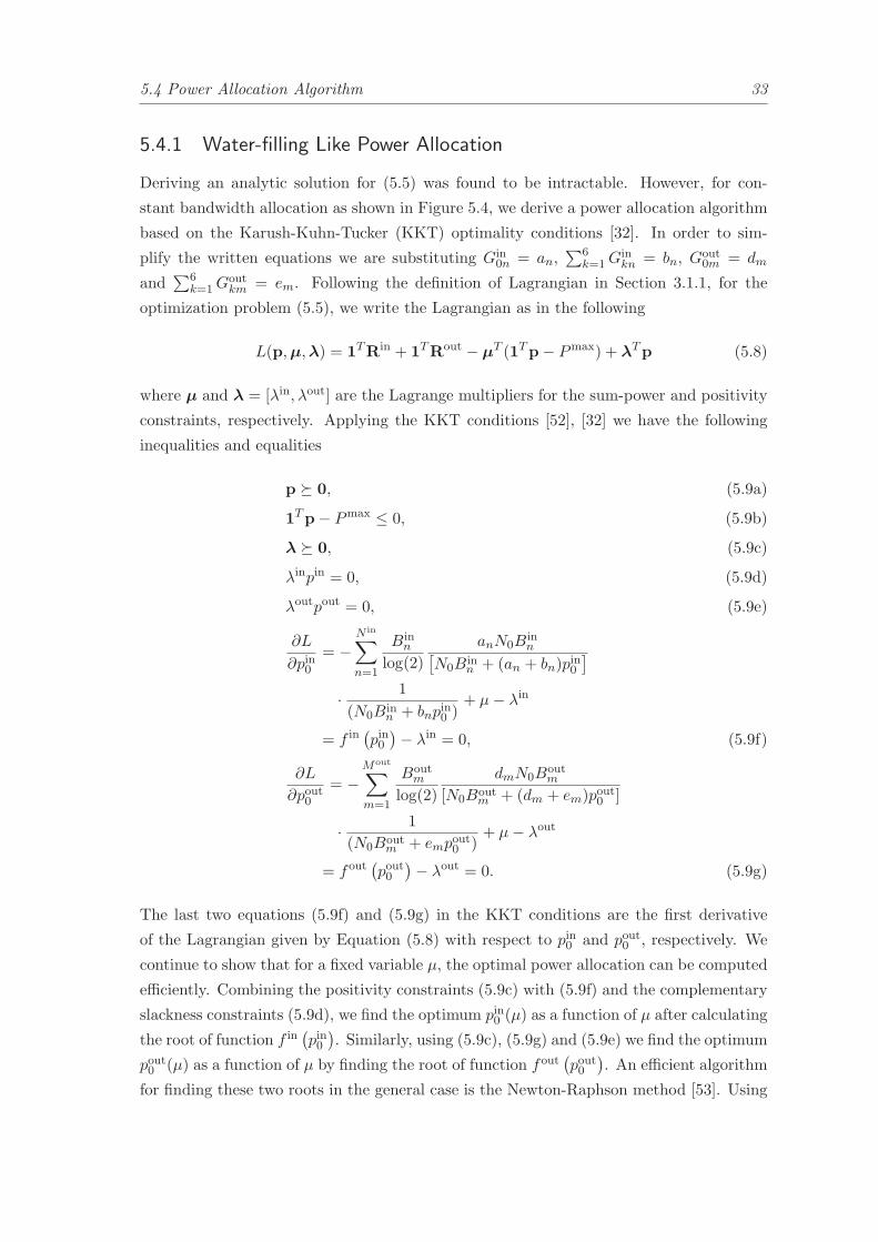
5.4 Power Allocation Algorithm 33
5.4.1 Water-filling Like Power Allocation
Deriving an analytic solution for (5.5) was found to be intractable. However, for con-
stant bandwidth allocation as shown in Figure 5.4, we derive a power allocation algorithm
based on the Karush-Kuhn-Tucker (KKT) optimality conditions [32]. In order to sim-
plify the written equations we are substituting Gin0n = an,
∑6k=1G
inkn = bn, G
out0m = dm
and∑6
k=1Goutkm = em. Following the definition of Lagrangian in Section 3.1.1, for the
optimization problem (5.5), we write the Lagrangian as in the following
L(p,µ,λ) = 1TRin + 1TRout − µT (1Tp− Pmax) + λTp (5.8)
where µ and λ = [λin, λout] are the Lagrange multipliers for the sum-power and positivity
constraints, respectively. Applying the KKT conditions [52], [32] we have the following
inequalities and equalities
p � 0, (5.9a)
1Tp− Pmax ≤ 0, (5.9b)
λ � 0, (5.9c)
λinpin = 0, (5.9d)
λoutpout = 0, (5.9e)
∂L
∂pin0= −
N in∑
n=1
Binn
log(2)
anN0Binn
[
N0Binn + (an + bn)pin0
]
· 1
(N0Binn + bnpin0 )
+ µ− λin
= f in(
pin0)
− λin = 0, (5.9f)
∂L
∂pout0
= −Mout∑
m=1
Boutm
log(2)
dmN0Boutm
[N0Boutm + (dm + em)pout0 ]
· 1
(N0Boutm + empout0 )
+ µ− λout
= fout(
pout0
)
− λout = 0. (5.9g)
The last two equations (5.9f) and (5.9g) in the KKT conditions are the first derivative
of the Lagrangian given by Equation (5.8) with respect to pin0 and pout0 , respectively. We
continue to show that for a fixed variable µ, the optimal power allocation can be computed
efficiently. Combining the positivity constraints (5.9c) with (5.9f) and the complementary
slackness constraints (5.9d), we find the optimum pin0 (µ) as a function of µ after calculating
the root of function f in(
pin0)
. Similarly, using (5.9c), (5.9g) and (5.9e) we find the optimum
pout0 (µ) as a function of µ by finding the root of function fout(
pout0
)
. An efficient algorithm
for finding these two roots in the general case is the Newton-Raphson method [53]. Using
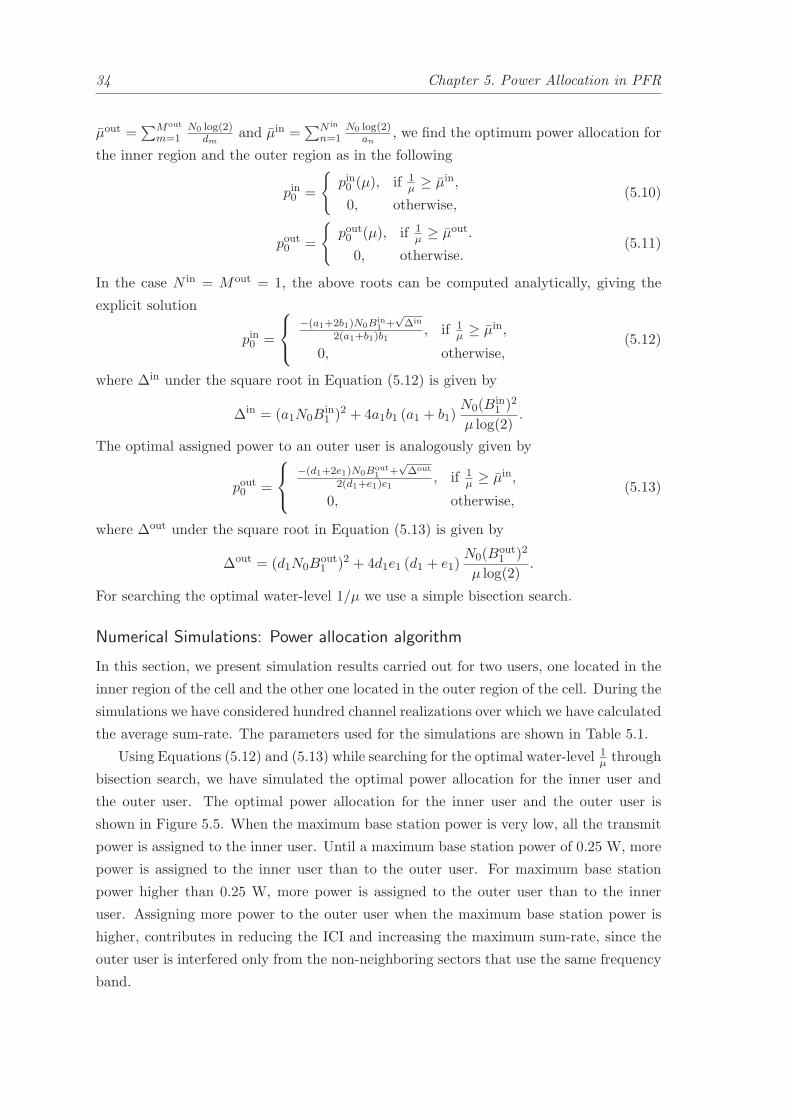
34 Chapter 5. Power Allocation in PFR
µout =∑Mout
m=1N0 log(2)
dmand µin =
∑N in
n=1N0 log(2)
an, we find the optimum power allocation for
the inner region and the outer region as in the following
pin0 =
{
pin0 (µ), if 1µ ≥ µin,
0, otherwise,(5.10)
pout0 =
{
pout0 (µ), if 1µ ≥ µout.
0, otherwise.(5.11)
In the case N in = Mout = 1, the above roots can be computed analytically, giving the
explicit solution
pin0 =
−(a1+2b1)N0Bin1+√∆in
2(a1+b1)b1, if 1
µ ≥ µin,
0, otherwise,(5.12)
where ∆in under the square root in Equation (5.12) is given by
∆in = (a1N0Bin1 )2 + 4a1b1 (a1 + b1)
N0(Bin1 )2
µ log(2).
The optimal assigned power to an outer user is analogously given by
pout0 =
−(d1+2e1)N0Bout1
+√∆out
2(d1+e1)e1, if 1
µ ≥ µin,
0, otherwise,(5.13)
where ∆out under the square root in Equation (5.13) is given by
∆out = (d1N0Bout1 )2 + 4d1e1 (d1 + e1)
N0(Bout1 )2
µ log(2).
For searching the optimal water-level 1/µ we use a simple bisection search.
Numerical Simulations: Power allocation algorithm
In this section, we present simulation results carried out for two users, one located in the
inner region of the cell and the other one located in the outer region of the cell. During the
simulations we have considered hundred channel realizations over which we have calculated
the average sum-rate. The parameters used for the simulations are shown in Table 5.1.
Using Equations (5.12) and (5.13) while searching for the optimal water-level 1µ through
bisection search, we have simulated the optimal power allocation for the inner user and
the outer user. The optimal power allocation for the inner user and the outer user is
shown in Figure 5.5. When the maximum base station power is very low, all the transmit
power is assigned to the inner user. Until a maximum base station power of 0.25 W, more
power is assigned to the inner user than to the outer user. For maximum base station
power higher than 0.25 W, more power is assigned to the outer user than to the inner
user. Assigning more power to the outer user when the maximum base station power is
higher, contributes in reducing the ICI and increasing the maximum sum-rate, since the
outer user is interfered only from the non-neighboring sectors that use the same frequency
band.

5.4 Power Allocation Algorithm 35
Table 5.1: Simulation parameters
parameters value
Maximum base station power Pmax 5 W
Maximum base station bandwidth Bmax 20 MHz
Noise spectral density N0 −174 dBm/Hz
Center frequency f 2.0 GHz
Pathloss exponent α 3.75
Penetration loss Lp 20 dB
Shadowing Xσ N (0, 8)dB
Small-scale Fading F χ22 dB,
Inter base station distance d 700 m
Position of inner user in polar coordinates (120 m, 1600)
Position of outer user in polar coordinates (370 m, 1600)
0 1 2 3 4 50
0.5
1
1.5
2
2.5
3
3.5
Maximum base station power [W]
Assig
ned p
ow
er
for
inner
and o
ute
r users
[W
]
0 0.2 0.4 0.6 0.80
0.1
0.2
0.3
0.4
0.5
0.6
Power assignment to the outer user
Power assignment to the inner user
Figure 5.5: Optimal power assignment to the inner and outer users
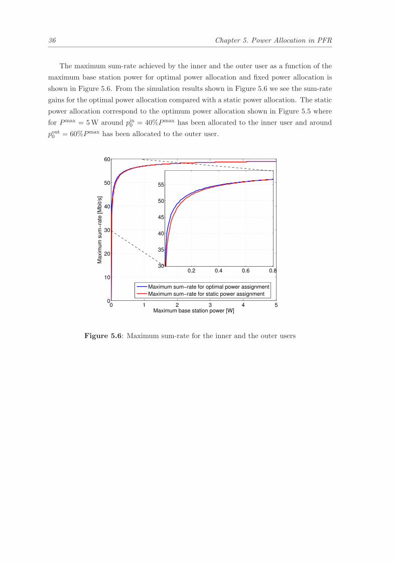
36 Chapter 5. Power Allocation in PFR
The maximum sum-rate achieved by the inner and the outer user as a function of the
maximum base station power for optimal power allocation and fixed power allocation is
shown in Figure 5.6. From the simulation results shown in Figure 5.6 we see the sum-rate
gains for the optimal power allocation compared with a static power allocation. The static
power allocation correspond to the optimum power allocation shown in Figure 5.5 where
for Pmax = 5W around pin0 = 40%Pmax has been allocated to the inner user and around
pout0 = 60%Pmax has been allocated to the outer user.
0 1 2 3 4 50
10
20
30
40
50
60
Maximum base station power [W]
Maxim
um
sum
−ra
te [M
bit/s
]
0.2 0.4 0.6 0.830
35
40
45
50
55
Maximum sum−rate for optimal power assignment
Maximum sum−rate for static power assignment
Figure 5.6: Maximum sum-rate for the inner and the outer users

5.5 Power Allocation Algorithms in Convex Form 37
5.5 Power Allocation Algorithms in Convex Form
In this section, two different types of optimization problems for systems employing the
PFR and performing power and bandwidth allocation jointly are studied. Without relying
on any assumptions on power allocations as in Section 5.4, we proof that these problems
can be transformed into GP convex ones and hence solved efficiently using state-of-the-art
convex optimization methods [32].
5.5.1 Maximization of the Minimum Rate in Convex Form
The problem of maximizing the minimum rate among all users in all cells in GGP form is
formulated in the following:
maximizeβin,βout,tin,tout∈R+,p�0
min{βintin log(2), βouttout log(2)} (5.14a)
subject to
tin ≤ log
(
1 +pinc
ninu β
in +∑
k∈C\c ginkup
ink
)
, ∀u ∈ U inc ,
∀c ∈ C, (5.14b)
tout ≤ log
(
1 +poutc
noutu βout +
∑
k∈C\c goutku poutk
)
, ∀u ∈ Uoutc ,
∀c ∈ C, (5.14c)
βin + βout ≤ 1, (5.14d)
pinc + poutc ≤ Pmaxc , ∀c ∈ C, (5.14e)
where βin, βout, tin and tout are the normalized bandwidths and minimum rates allo-
cated to inner and outer users, respectively. The subscripts u and c denote the user
and cell, the calligraphies U and C denote the set of users and the set of cells. Further-
more, ninu = N0u/G
inu and ginku = Gin
ku/Ginu are the normalized noise and the normalized
interference channel LSPLA for the inner users, respectively. Similar to the inner users
noutu = N0u/G
outu and goutku = Gout
ku /Goutu are the normalized noise and the normalized
interference channel LSPLA for the outer users.
Proposition 1. The max-min-rate problem ( 5.14) can be transformed into a GP convex
optimization problem.
Proof. We begin by exchanging the objective in (5.14a) by its logarithm which notably
does not change the optimal variables. Introducing several variable transformations tin =
log(etin − 1), tout = log(et
out − 1), βin = log(βin), βout = log(βout), pinc = log(pinc ) and
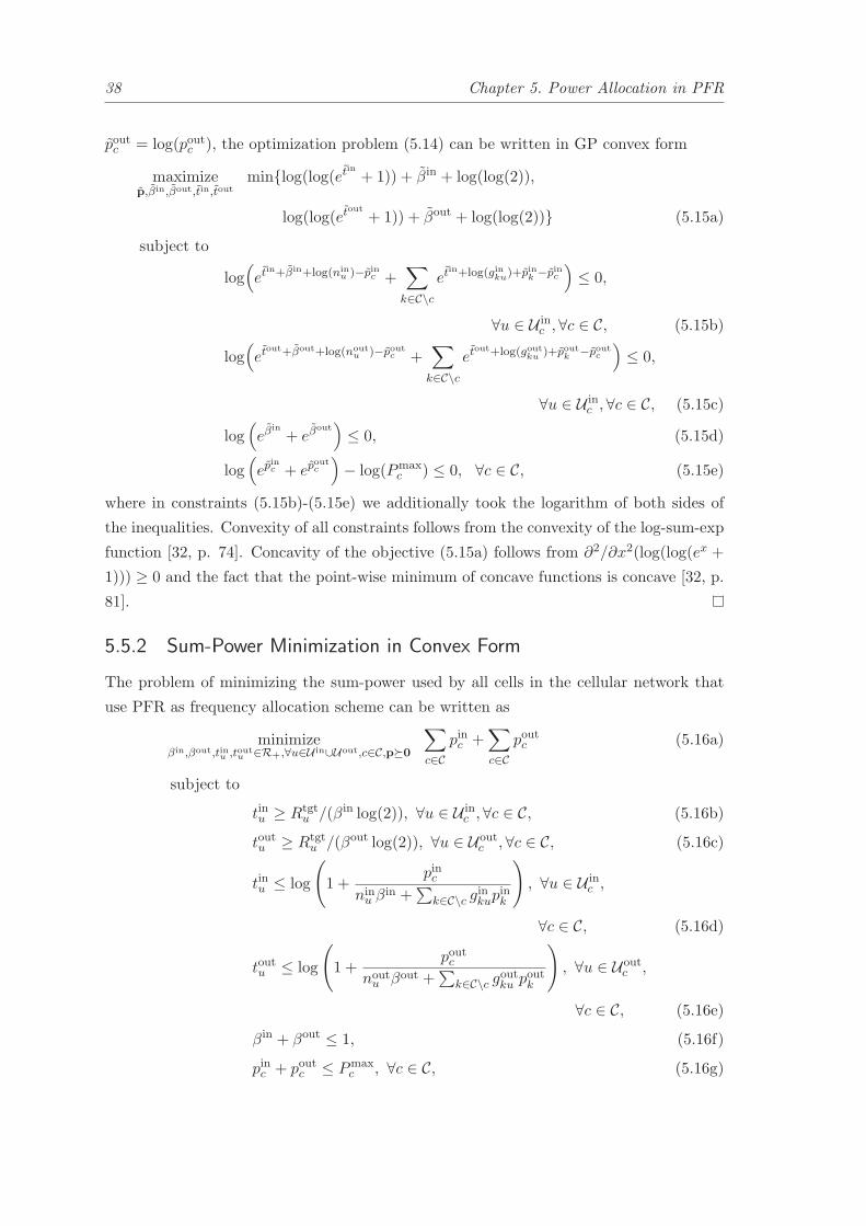
38 Chapter 5. Power Allocation in PFR
poutc = log(poutc ), the optimization problem (5.14) can be written in GP convex form
maximizep,βin,βout,tin,tout
min{log(log(etin + 1)) + βin + log(log(2)),
log(log(etout
+ 1)) + βout + log(log(2))} (5.15a)
subject to
log(
etin+βin+log(nin
u )−pinc +∑
k∈C\cet
in+log(ginku
)+pink−pinc
)
≤ 0,
∀u ∈ U inc , ∀c ∈ C, (5.15b)
log(
etout+βout+log(nout
u )−poutc +∑
k∈C\cet
out+log(goutku
)+poutk
−poutc
)
≤ 0,
∀u ∈ U inc , ∀c ∈ C, (5.15c)
log(
eβin
+ eβout)
≤ 0, (5.15d)
log(
epinc + ep
outc
)
− log(Pmaxc ) ≤ 0, ∀c ∈ C, (5.15e)
where in constraints (5.15b)-(5.15e) we additionally took the logarithm of both sides of
the inequalities. Convexity of all constraints follows from the convexity of the log-sum-exp
function [32, p. 74]. Concavity of the objective (5.15a) follows from ∂2/∂x2(log(log(ex +
1))) ≥ 0 and the fact that the point-wise minimum of concave functions is concave [32, p.
81].
5.5.2 Sum-Power Minimization in Convex Form
The problem of minimizing the sum-power used by all cells in the cellular network that
use PFR as frequency allocation scheme can be written as
minimizeβin,βout,tinu ,toutu ∈R+,∀u∈U in∪Uout,c∈C,p�0
∑
c∈Cpinc +
∑
c∈Cpoutc (5.16a)
subject to
tinu ≥ Rtgtu /(βin log(2)), ∀u ∈ U in
c , ∀c ∈ C, (5.16b)
toutu ≥ Rtgtu /(βout log(2)), ∀u ∈ Uout
c , ∀c ∈ C, (5.16c)
tinu ≤ log
(
1 +pinc
ninu β
in +∑
k∈C\c ginkup
ink
)
, ∀u ∈ U inc ,
∀c ∈ C, (5.16d)
toutu ≤ log
(
1 +poutc
noutu βout +
∑
k∈C\c goutku poutk
)
, ∀u ∈ Uoutc ,
∀c ∈ C, (5.16e)
βin + βout ≤ 1, (5.16f)
pinc + poutc ≤ Pmaxc , ∀c ∈ C, (5.16g)
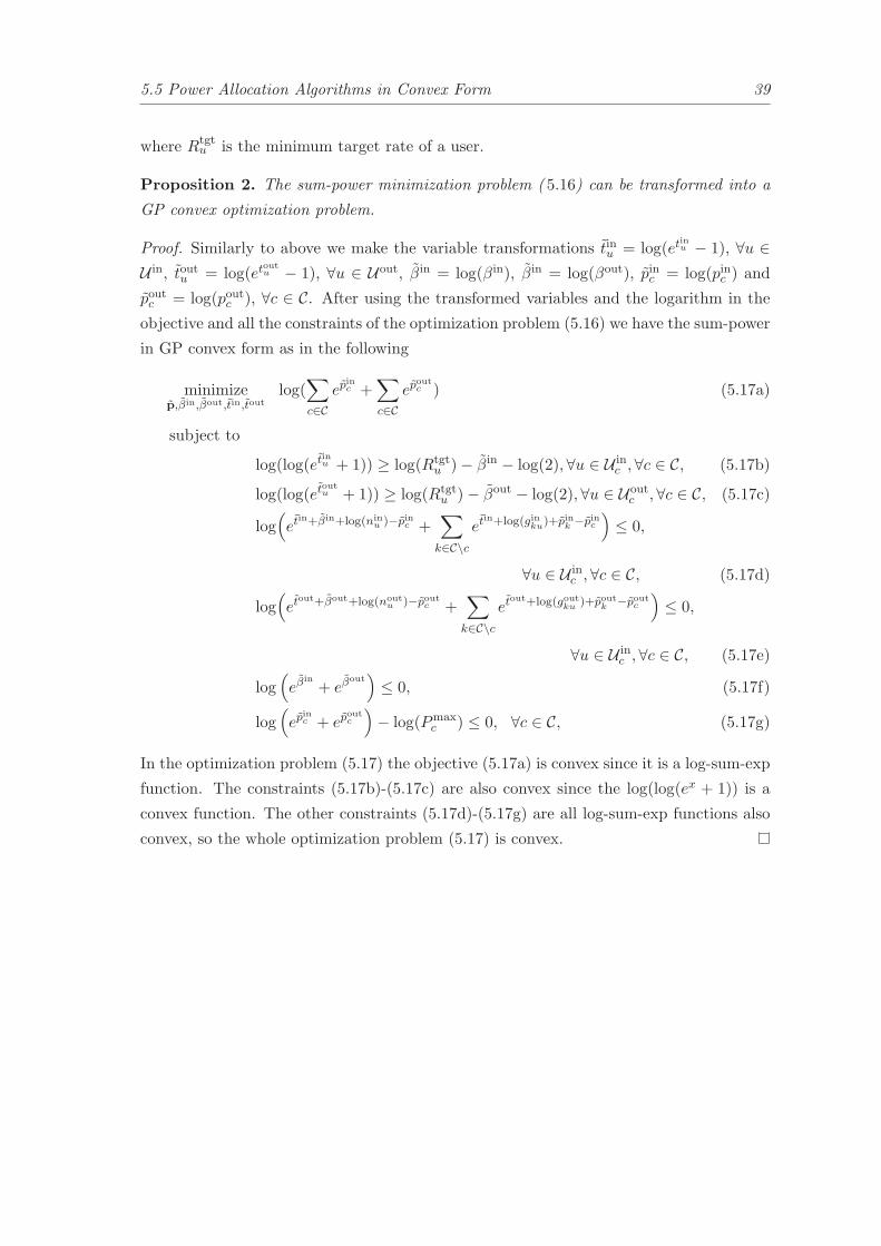
5.5 Power Allocation Algorithms in Convex Form 39
where Rtgtu is the minimum target rate of a user.
Proposition 2. The sum-power minimization problem ( 5.16) can be transformed into a
GP convex optimization problem.
Proof. Similarly to above we make the variable transformations tinu = log(etinu − 1), ∀u ∈
U in, toutu = log(etoutu − 1), ∀u ∈ Uout, βin = log(βin), βin = log(βout), pinc = log(pinc ) and
poutc = log(poutc ), ∀c ∈ C. After using the transformed variables and the logarithm in the
objective and all the constraints of the optimization problem (5.16) we have the sum-power
in GP convex form as in the following
minimizep,βin,βout,tin,tout
log(∑
c∈Cep
inc +
∑
c∈Cep
outc ) (5.17a)
subject to
log(log(etinu + 1)) ≥ log(Rtgt
u )− βin − log(2), ∀u ∈ U inc , ∀c ∈ C, (5.17b)
log(log(etoutu + 1)) ≥ log(Rtgt
u )− βout − log(2), ∀u ∈ Uoutc , ∀c ∈ C, (5.17c)
log(
etin+βin+log(nin
u )−pinc +∑
k∈C\cet
in+log(ginku
)+pink−pinc
)
≤ 0,
∀u ∈ U inc , ∀c ∈ C, (5.17d)
log(
etout+βout+log(nout
u )−poutc +∑
k∈C\cet
out+log(goutku
)+poutk
−poutc
)
≤ 0,
∀u ∈ U inc , ∀c ∈ C, (5.17e)
log(
eβin
+ eβout)
≤ 0, (5.17f)
log(
epinc + ep
outc
)
− log(Pmaxc ) ≤ 0, ∀c ∈ C, (5.17g)
In the optimization problem (5.17) the objective (5.17a) is convex since it is a log-sum-exp
function. The constraints (5.17b)-(5.17c) are also convex since the log(log(ex + 1)) is a
convex function. The other constraints (5.17d)-(5.17g) are all log-sum-exp functions also
convex, so the whole optimization problem (5.17) is convex.

6Bandwidth and Power
Allocation in Partial
Frequency Reuse
OPTIMIZING only the power allocation while considering the bandwidth allocation
fixed is not the most efficient solution. Considering that bandwidth resources are
very expensive and also limited, it is necessary to optimize such resources. In this chapter,
I show the application of optimal power allocation algorithm for bandwidth re-allocation
scheme. Furthermore, I present the optimization of the bandwidth allocation jointly with
power allocation. Due to complexity in finding solutions for jointly bandwidth and power
allocation, in this chapter we present the optimization of power allocation and bandwidth
adaption in cell region based on users classification.
In Section 6.1 a variable bandwidth and variable power allocation scheme is shown.
Using this scheme in Section 6.2, the bandwidth and power allocation algorithms for PFR
in GP form are formulated.
In Section 6.3 the bandwidth re-allocation scheme is shown for PFR. Applying such
scheme we obtain the results in power allocation and sum-rate maximization for two cases
of users classification: classification by distance threshold and by LSPLA threshold. Fur-
thermore in Section 6.4, considering the mean LSPLA as threshold for users classification,
we have formulated two other algorithms for PFR. The optimal power and adaptive
bandwidth algorithm, which adapts the bandwidth allocation based on the users classi-
fication, while optimizing the power allocation using the maximization of the minimum
SINR. Using such algorithm, we have shown the optimality of PFR in power allocation.
41
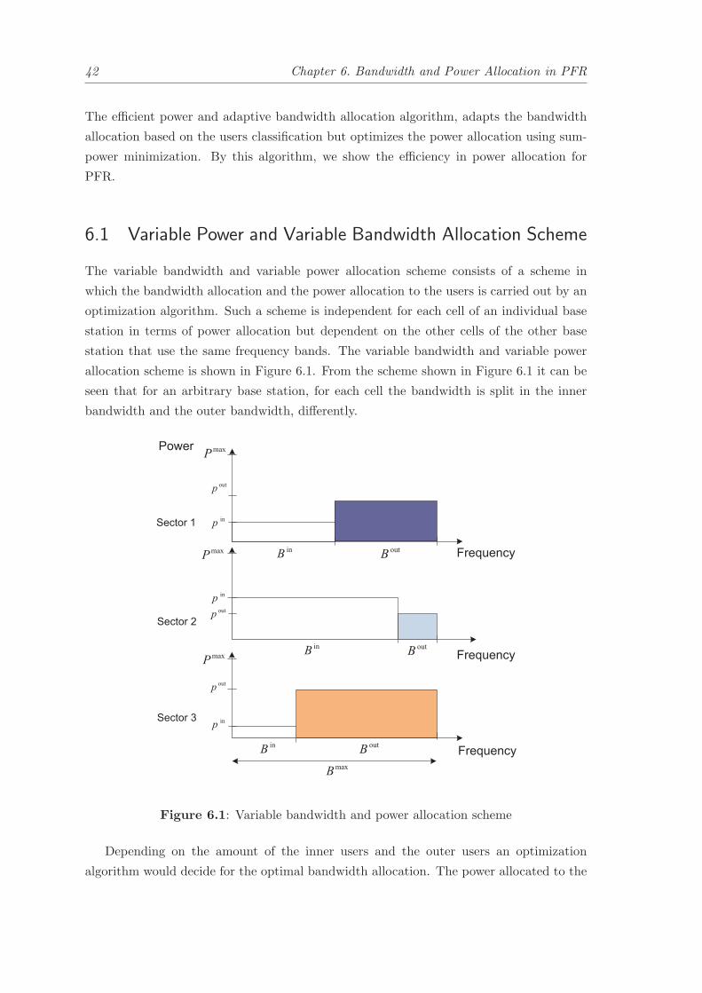
42 Chapter 6. Bandwidth and Power Allocation in PFR
The efficient power and adaptive bandwidth allocation algorithm, adapts the bandwidth
allocation based on the users classification but optimizes the power allocation using sum-
power minimization. By this algorithm, we show the efficiency in power allocation for
PFR.
6.1 Variable Power and Variable Bandwidth Allocation Scheme
The variable bandwidth and variable power allocation scheme consists of a scheme in
which the bandwidth allocation and the power allocation to the users is carried out by an
optimization algorithm. Such a scheme is independent for each cell of an individual base
station in terms of power allocation but dependent on the other cells of the other base
station that use the same frequency bands. The variable bandwidth and variable power
allocation scheme is shown in Figure 6.1. From the scheme shown in Figure 6.1 it can be
seen that for an arbitrary base station, for each cell the bandwidth is split in the inner
bandwidth and the outer bandwidth, differently.
inp
outp
inB
outB
maxB
Frequency
maxP
inpoutp
inB out
B Frequency
maxP
inp
outp
inB out
B Frequency
Power maxP
Sector 1
Sector 3
Sector 2
Figure 6.1: Variable bandwidth and power allocation scheme
Depending on the amount of the inner users and the outer users an optimization
algorithm would decide for the optimal bandwidth allocation. The power allocated to the

6.2 Bandwidth and Power Allocation Algorithms 43
inner users is different from the power allocated to the outer users. For each individual
cell the sum of the bandwidths allocated to the inner users and to the outer users is equal
to the maximum cell bandwidth. This is due to the optimality. On the other hand the
sum of the power allocation is equal to the maximum base station power only in case of
an optimal optimization algorithm for power allocation.
6.2 Bandwidth and Power Allocation Algorithms
The optimization algorithms for bandwidth and power allocation are formulated to satisfy
the users requests for transmission rate with radio resource that we have. The algorithms
that we show in the following use joint optimization of bandwidth and power allocation in
PFR to optimally allocate the bandwidth to the users and efficiently allocate the power
in the cell regions. The optimization problem which is optimal for the bandwidth alloca-
tion and sub-optimal for power allocation in PFR, is the maximization of the minimum
rate. Applying such optimization problem, we formulated efficient algorithms for users
classification in the cell regions.
6.2.1 Maximization of the Minimum Rate
In this section, the maximization of the minimum rate for systems employing PFR and
performing power allocation and bandwidth allocation is studied. Without relying on any
assumptions on power allocations or high-SINR approximation, we have proven that such
optimization problem can be transformed into GP optimization problem and hence solved
efficiently using Disciplined Convex Programming (DCP) methods. The maximization of
the minimum rate offers flexibility in solving joint bandwidth and power allocation for
multiple users over multiple cells. The problem of maximizing the minimum rate among
all users in all cells for PFR cellular network is written in the following

44 Chapter 6. Bandwidth and Power Allocation in PFR
maximizeβincn,β
outcm∈R+,p�0
min{βinc1t
in log(2), ..., βincNint
in log(2),
βoutc1 tout log(2), ..., βout
cMouttout log(2)} (6.1a)
subject to
tin ≤ log
(
1 +pinc
nin1 β
inc1 +
∑
k∈C\c gink1p
ink
)
, ∀c ∈ C, (6.1b)
...
tin ≤ log
(
1 +pinc
ninNinβ
incNin +
∑
k∈C\c ginkNinp
ink
)
, ∀c ∈ C, (6.1c)
tout ≤ log
(
1 +poutc
nout1 βout
c1 +∑
k∈C\c goutk1 poutk
)
, ∀c ∈ C, (6.1d)
...
tout ≤ log
(
1 +poutc
noutMoutβout
cMout +∑
k∈C\c goutkMoutpoutk
)
, ∀c ∈ C, (6.1e)
Nin∑
n=1
βincn +
Mout∑
m=1
βoutcm ≤ 1, ∀c ∈ C (6.1f)
pinc + poutc ≤ Pmaxc , ∀c ∈ C, (6.1g)
As we have introduced in Section 3.2.1, the optimization problem of maximizing the min-
imum rate written by Equation (6.1) is in GGP form. In the optimization problem (6.1),
the constraints (6.1b)-(6.1c) show the normalized inner user rates which are constrained
by normalized minimum required inner user rate. Similarly for the outer users, the con-
straints (6.1d)-(6.1e) apply. The last two constraints (6.1f) and (6.1g) are the bandwidth
and the power constraints.
Proposition 3. The max-min-rate problem ( 6.1) can be transformed into GP optimization
problem.
Proof. Similar to the maximization of the minimum posynomials explained in Section 3.2.1,
we begin by introducing a variable z which act lower bound [36] in the objective (6.1a)
and by using its inverse in the objective we convert the GGP into a GP [37]. Applying
exponential in both sides of constraints (6.1b)-(6.1e), which notably does not change the
optimal variables, converts the optimization problem (6.1) into a GP, where CVX can be
used to get the optimal bandwidth allocation and sub-optimal power allocation. Now the
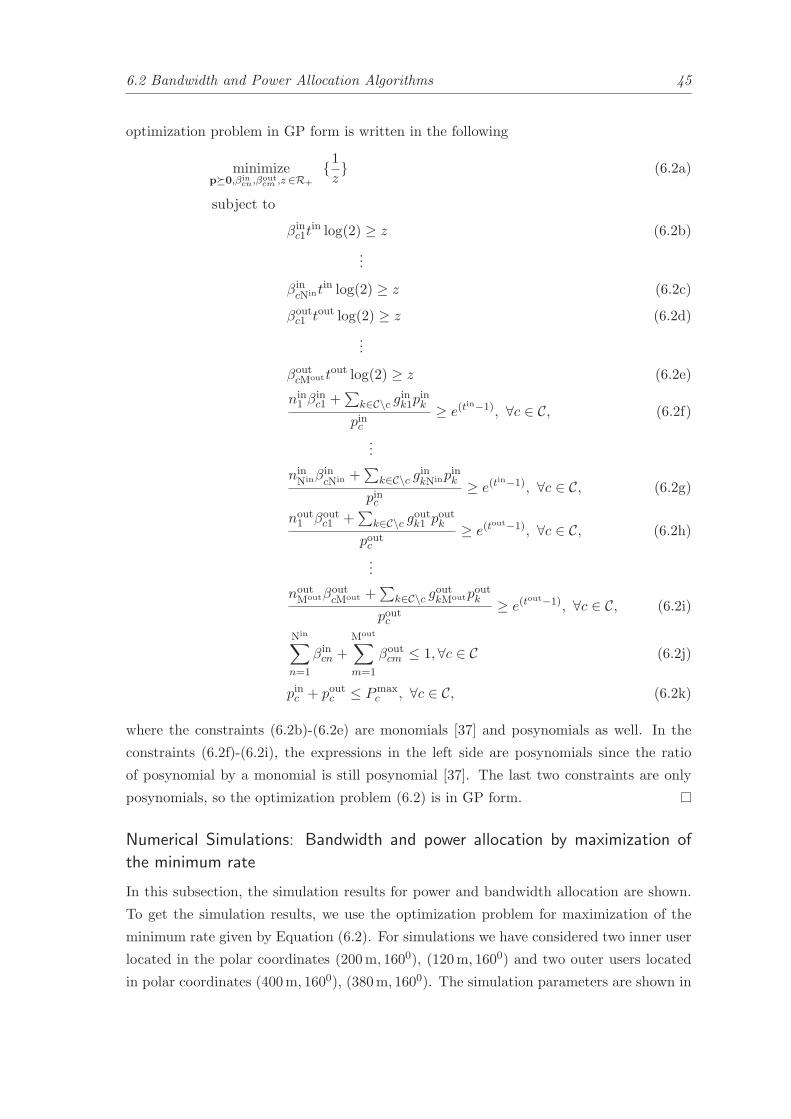
6.2 Bandwidth and Power Allocation Algorithms 45
optimization problem in GP form is written in the following
minimizep�0,βin
cn,βoutcm ,z ∈R+
{1z} (6.2a)
subject to
βinc1t
in log(2) ≥ z (6.2b)
...
βincNint
in log(2) ≥ z (6.2c)
βoutc1 tout log(2) ≥ z (6.2d)
...
βoutcMouttout log(2) ≥ z (6.2e)
nin1 β
inc1 +
∑
k∈C\c gink1p
ink
pinc≥ e(t
in−1), ∀c ∈ C, (6.2f)
...
ninNinβ
incNin +
∑
k∈C\c ginkNinp
ink
pinc≥ e(t
in−1), ∀c ∈ C, (6.2g)
nout1 βout
c1 +∑
k∈C\c goutk1 poutk
poutc
≥ e(tout−1), ∀c ∈ C, (6.2h)
...
noutMoutβout
cMout +∑
k∈C\c goutkMoutpoutk
poutc
≥ e(tout−1), ∀c ∈ C, (6.2i)
Nin∑
n=1
βincn +
Mout∑
m=1
βoutcm ≤ 1, ∀c ∈ C (6.2j)
pinc + poutc ≤ Pmaxc , ∀c ∈ C, (6.2k)
where the constraints (6.2b)-(6.2e) are monomials [37] and posynomials as well. In the
constraints (6.2f)-(6.2i), the expressions in the left side are posynomials since the ratio
of posynomial by a monomial is still posynomial [37]. The last two constraints are only
posynomials, so the optimization problem (6.2) is in GP form.
Numerical Simulations: Bandwidth and power allocation by maximization of
the minimum rate
In this subsection, the simulation results for power and bandwidth allocation are shown.
To get the simulation results, we use the optimization problem for maximization of the
minimum rate given by Equation (6.2). For simulations we have considered two inner user
located in the polar coordinates (200m, 1600), (120m, 1600) and two outer users located
in polar coordinates (400m, 1600), (380m, 1600). The simulation parameters are shown in
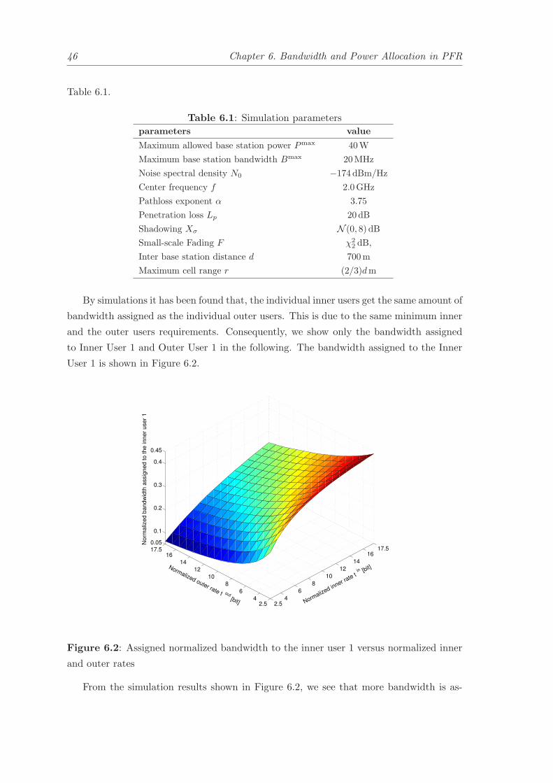
46 Chapter 6. Bandwidth and Power Allocation in PFR
Table 6.1.
Table 6.1: Simulation parameters
parameters value
Maximum allowed base station power Pmax 40W
Maximum base station bandwidth Bmax 20MHz
Noise spectral density N0 −174 dBm/Hz
Center frequency f 2.0GHz
Pathloss exponent α 3.75
Penetration loss Lp 20 dB
Shadowing Xσ N (0, 8) dB
Small-scale Fading F χ22 dB,
Inter base station distance d 700m
Maximum cell range r (2/3)dm
By simulations it has been found that, the individual inner users get the same amount of
bandwidth assigned as the individual outer users. This is due to the same minimum inner
and the outer users requirements. Consequently, we show only the bandwidth assigned
to Inner User 1 and Outer User 1 in the following. The bandwidth assigned to the Inner
User 1 is shown in Figure 6.2.
2.54
6
8
10
12
14
1617.5
2.54
6
8
10
12
14
1617.50.05
0.1
0.2
0.3
0.4
0.45
Normalized in
ner rate t
in [bit]Normalized outer rate t out
[bit]
No
rma
lize
d b
an
dw
idth
assig
ne
d t
o t
he
in
ne
r u
se
r 1
Figure 6.2: Assigned normalized bandwidth to the inner user 1 versus normalized inner
and outer rates
From the simulation results shown in Figure 6.2, we see that more bandwidth is as-
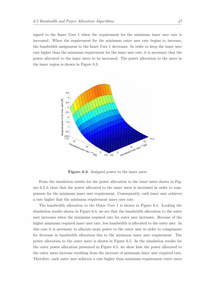
6.2 Bandwidth and Power Allocation Algorithms 47
signed to the Inner User 1 when the requirement for the minimum inner user rate is
increased. When the requirement for the minimum outer user rate begins to increase,
the bandwidth assignment to the Inner User 1 decreases. In order to keep the inner user
rate higher than the minimum requirement for the inner user rate, it is necessary that the
power allocated to the inner users to be increased. The power allocation to the users in
the inner region is shown in Figure 6.3.
2.5
5
10
15
17.5
2.5
5
10
15
17.50.03
0.5
1
1.5
2
2.5
3
3.5
4
4.5
Normalized inner rate t
in [bit]Normalized outer rate t out
[bit]
Assig
ne
d p
ow
er
to t
he
in
ne
r u
se
rs [
W]
Figure 6.3: Assigned power to the inner users
From the simulation results for the power allocation to the inner users shown in Fig-
ure 6.3 it clear that the power allocated to the inner users is increased in order to com-
pensate for the minimum inner user requirement. Consequently, each inner user achieves
a rate higher that the minimum requirement inner user rate.
The bandwidth allocation to the Outer User 1 is shown in Figure 6.4. Looking the
simulation results shown in Figure 6.4, we see that the bandwidth allocation to the outer
user increases when the minimum required rate for outer user increases. Because of the
higher minimum required inner user rate, less bandwidth is allocated to the outer user. In
this case it is necessary to allocate more power to the outer user in order to compensate
for decrease in bandwidth allocation due to the minimum inner user requirement. The
power allocation to the outer users is shown in Figure 6.5. In the simulation results for
the outer power allocation presented in Figure 6.5, we show how the power allocated to
the outer users increase resulting from the increase of minimum inner user required rate.
Therefore, each outer user achieves a rate higher than minimum requirement outer users
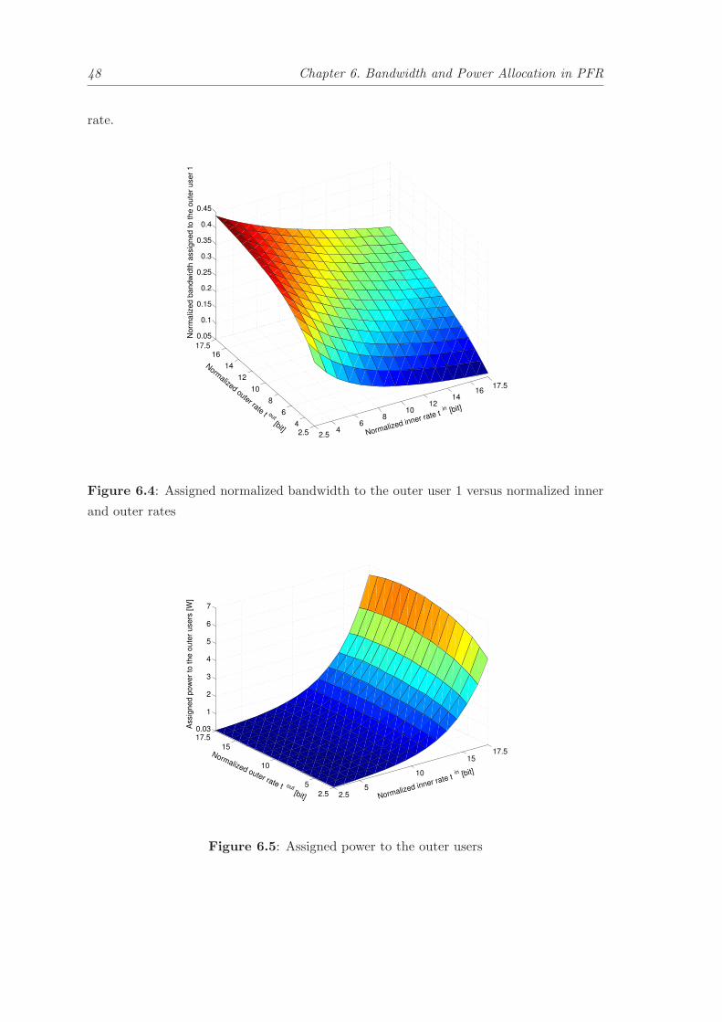
48 Chapter 6. Bandwidth and Power Allocation in PFR
rate.
2.54
68
1012
1416
17.5
2.54
6
8
10
12
14
1617.5
0.05
0.1
0.15
0.2
0.25
0.3
0.35
0.4
0.45
Normalized inner rate t in [bit]
Normalized outer rate t out
[bit]
No
rma
lize
d b
an
dw
idth
assig
ne
d t
o t
he
ou
ter
use
r 1
Figure 6.4: Assigned normalized bandwidth to the outer user 1 versus normalized inner
and outer rates
2.55
10
1517.5
2.5
5
10
15
17.50.03
1
2
3
4
5
6
7
Normalized inner rate t in [bit]
Normalized outer rate t out [bit]
Assig
ne
d p
ow
er
to t
he
ou
ter
use
rs [
W]
Figure 6.5: Assigned power to the outer users
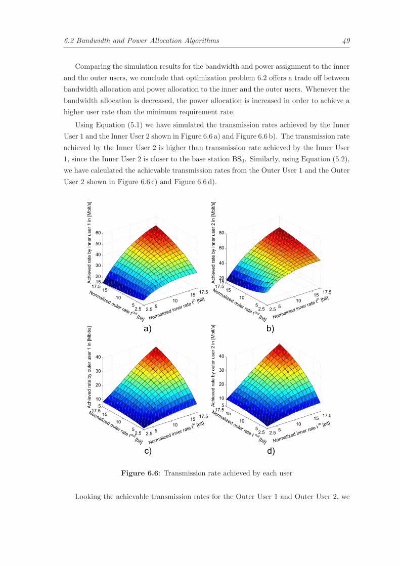
6.2 Bandwidth and Power Allocation Algorithms 49
Comparing the simulation results for the bandwidth and power assignment to the inner
and the outer users, we conclude that optimization problem 6.2 offers a trade off between
bandwidth allocation and power allocation to the inner and the outer users. Whenever the
bandwidth allocation is decreased, the power allocation is increased in order to achieve a
higher user rate than the minimum requirement rate.
Using Equation (5.1) we have simulated the transmission rates achieved by the Inner
User 1 and the Inner User 2 shown in Figure 6.6 a) and Figure 6.6 b). The transmission rate
achieved by the Inner User 2 is higher than transmission rate achieved by the Inner User
1, since the Inner User 2 is closer to the base station BS0. Similarly, using Equation (5.2),
we have calculated the achievable transmission rates from the Outer User 1 and the Outer
User 2 shown in Figure 6.6 c) and Figure 6.6 d).
2.55
10
1517.5
2.55
10
1517.5
1520
30
40
50
60
Normalized inner rate t
in [bit]
Normalized outer rate t out[bit]
Achie
ved r
ate
by inner
user
1 in [M
bit/s
]
2.55
10
1517.5
2.55
10
1517.5
1520
40
60
80
Normalized inner rate t
in [bit]
Normalized outer rate t out[bit]
Achie
ved r
ate
by inner
user
2 in [M
bit/s
]
2.55
10
1517.5
2.55
10
1517.5
5
10
20
30
40
Normalized inner rate t
in [bit]
Normalized outer rate t out[bit]
Achie
ved r
ate
by o
ute
r user
1 in [M
bit/s
]
2.55
10
1517.5
2.55
10
1517.5
5
10
20
30
40
Normalized inner rate tin [bit]
Normalized outer rate t out[bit]
Achie
ved r
ate
by o
ute
r user
2 in [M
bit/s
]
a) b)
c) d)
Figure 6.6: Transmission rate achieved by each user
Looking the achievable transmission rates for the Outer User 1 and Outer User 2, we
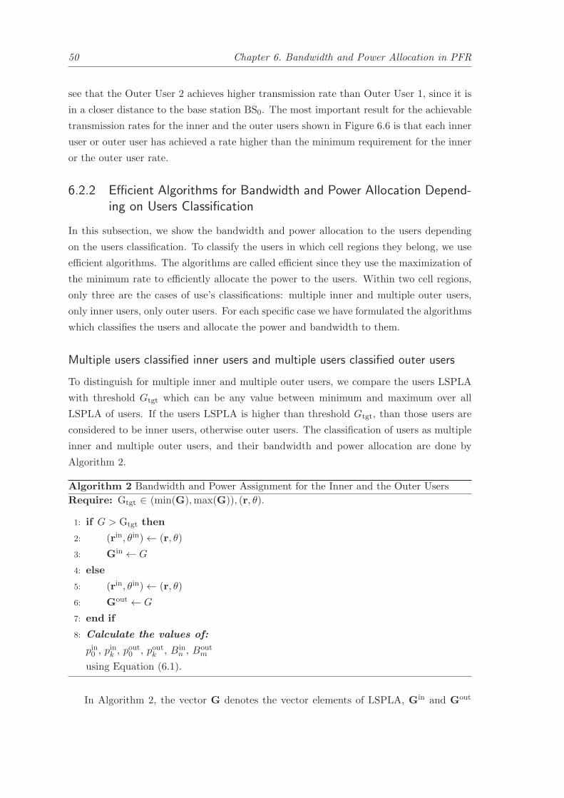
50 Chapter 6. Bandwidth and Power Allocation in PFR
see that the Outer User 2 achieves higher transmission rate than Outer User 1, since it is
in a closer distance to the base station BS0. The most important result for the achievable
transmission rates for the inner and the outer users shown in Figure 6.6 is that each inner
user or outer user has achieved a rate higher than the minimum requirement for the inner
or the outer user rate.
6.2.2 Efficient Algorithms for Bandwidth and Power Allocation Depend-ing on Users Classification
In this subsection, we show the bandwidth and power allocation to the users depending
on the users classification. To classify the users in which cell regions they belong, we use
efficient algorithms. The algorithms are called efficient since they use the maximization of
the minimum rate to efficiently allocate the power to the users. Within two cell regions,
only three are the cases of use’s classifications: multiple inner and multiple outer users,
only inner users, only outer users. For each specific case we have formulated the algorithms
which classifies the users and allocate the power and bandwidth to them.
Multiple users classified inner users and multiple users classified outer users
To distinguish for multiple inner and multiple outer users, we compare the users LSPLA
with threshold Gtgt which can be any value between minimum and maximum over all
LSPLA of users. If the users LSPLA is higher than threshold Gtgt, than those users are
considered to be inner users, otherwise outer users. The classification of users as multiple
inner and multiple outer users, and their bandwidth and power allocation are done by
Algorithm 2.
Algorithm 2 Bandwidth and Power Assignment for the Inner and the Outer Users
Require: Gtgt ∈ (min(G),max(G)), (r, θ).
1: if G > Gtgt then
2: (rin, θin)← (r, θ)
3: Gin ← G
4: else
5: (rin, θin)← (r, θ)
6: Gout ← G
7: end if
8: Calculate the values of:
pin0 , pink , p
out0 , poutk , Bin
n , Boutm
using Equation (6.1).
In Algorithm 2, the vector G denotes the vector elements of LSPLA, Gin and Gout

6.2 Bandwidth and Power Allocation Algorithms 51
denote the vector elements of LSPLA of the inner and the outer users, the (r, θ) denote the
vector elements of polar coordinates of users. Similarly (rin, θin) denote the vector elements
of polar coordinates for the inner users and (rout, θout) denote the vector elements of polar
coordinates for the outer users. The polar coordinates are included in all algorithms since
they present the locations of mobile users. Algorithm 2 requires the LSPLA threshold
to be defined for any value between the minimum and the maximum over all LSPLA of
users at the beginning. From the first to the sixth step, the Algorithm 2 classifies the
users to the inner and the outer regions. At the eight step, it uses the maximization of the
minimum rate given by Equation (6.2) to calculate the power and bandwidth allocation.
The transmission rates of the inner users can be calculated using Equation (5.1) and for
outer users similarly using Equation (5.2).
All users classified as inner users
To distinguish only for inner users, we define the LSPLA threshold Gtgt to be smaller than
all LSPLA of all users as it is shown in Algorithm 3.
Algorithm 3 Bandwidth and Power Assignment for the Inner Users
Require: Gtgt < min(G).
1: if G > Gtgt then
2: (rin, θin)← (r, θ)
3: Gin ← G
4: end if
5: Calculate the values of:
pin0 , pink , B
inn
using Equation (6.1).
From the first to third step it compares all LSPLA of the users with the threshold Gtgt
and classifies all users as inner users. In the last step runs the Equation (6.2) to calculate
the power and bandwidth assignment to the inner users. The transmission rate of inner
users are calculated using Equation (5.1).
All users classified as outer users
To distinguish only for outer users, the LSPLA threshold Gtgt is defined to be greater
than all LSPLA of users, as it is shown in Algorithm 4.
Similar to Algorithm 3, Algorithm 4 in the 1-3 step classifies all users as outer users by
comparing the users LSPLA with threshold Gtgt. In the last step uses the maximization
of the minimum rate given by Equation (6.2) to calculate the bandwidth and power as-
signed to the outer users. The transmission rates for the outer users are calculated using
Equation (5.2).

52 Chapter 6. Bandwidth and Power Allocation in PFR
Algorithm 4 Bandwidth and Power Assignment for the Outer Users
Require: Gtgt > max(G).
1: if G < Gtgt then
2: (rout, θout)← (r, θ)
3: Gout ← G
4: end if
5: Calculate the values of:
pout0 , poutk , Boutm
using Equation (6.1).
Numerical Simulations: Efficient Algorithms for Bandwidth and Power Alloca-
tion Depending on Users Classification
In this subsection, we show the simulation results carried out using the efficient algorithms
for classifying the users, and allocating the power and the bandwidth to the them. For
simulation uniform distances between users are considered, such that users are distributed
in a regular grid over the cell area. A realistic urban scenario is considered with its
parameters shown in Table 6.2.
Table 6.2: Simulation parameters
parameters value
Maximum base station power Pmaxc 40W
Maximum base station bandwidth Bmaxc 20MHz
Noise spectral density N0 −174 dBm/Hz
Center frequency f 2.0GHz
Path-loss exponent α 3.75
Penetration loss Lp 20 dB
Shadowing Xσ N (0, 8) dB
Small-scale fading F χ22 dB,
Inter base station distance d 600m
Minimum requirement inner user rate tin 2.5Mbit/s
Minimum requirement outer user rate tout 2.5Mbit/s
Number of active users within the cell 75
During simulations we have considered 100 realizations, where for each realizations
all users have experienced different channels due to shadowing and small-scale fading.
The efficiency of power allocation in terms of median values over those 100 realizations
versus the percentage of the inner users classification Nin [%] is shown in Figure 6.7. The
percentage of the outer users classification is thereby equivalent to 1−Nin [%]. Depending
on how we classify the users comparing with LSPLA threshold Gtgt, we define a direct
mapping of users classification to frequency reuse. Frequency reuse-1 is considered only
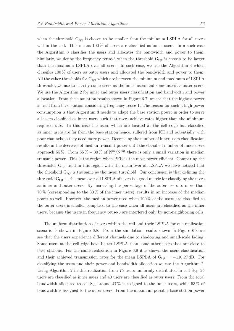
6.2 Bandwidth and Power Allocation Algorithms 53
when the threshold Gtgt is chosen to be smaller than the minimum LSPLA for all users
within the cell. This means 100% of users are classified as inner users. In a such case
the Algorithm 3 classifies the users and allocates the bandwidth and power to them.
Similarly, we define the frequency reuse-3 when the threshold Gtgt is chosen to be larger
than the maximum LSPLA over all users. In such case, we use the Algorithm 4 which
classifies 100% of users as outer users and allocated the bandwidth and power to them.
All the other thresholds for Gtgt which are between the minimum and maximum of LSPLA
threshold, we use to classify some users as the inner users and some users as outer users.
We use the Algorithm 2 for inner and outer users classification and bandwidth and power
allocation. From the simulation results shown in Figure 6.7, we see that the highest power
is used from base station considering frequency reuse-1. The reason for such a high power
consumption is that Algorithm 3 needs to adapt the base station power in order to serve
all users classified as inner users such that users achieve rates higher than the minimum
required rate. In this case the users which are located at the cell edge but classified
as inner users are far from the base station hence, suffered from ICI and potentially with
poor channels so they need more power. Decreasing the number of inner users classification
results in the decrease of median transmit power until the classified number of inner users
approach 55%. From 55% − 30% of Nin/Nout there is only a small variation in median
transmit power. This is the region when PFR is the most power efficient. Comparing the
thresholds Gtgt used in this region with the mean over all LSPLA we have noticed that
the threshold Gtgt is the same as the mean threshold. Our conclusion is that defining the
threshold Gtgt as the mean over all LSPLA of users is a good metric for classifying the users
as inner and outer users. By increasing the percentage of the outer users to more than
70% (corresponding to the 30% of the inner users), results in an increase of the median
power as well. However, the median power used when 100% of the users are classified as
the outer users is smaller compared to the case when all users are classified as the inner
users, because the users in frequency reuse-3 are interfered only by non-neighboring cells.
The uniform distribution of users within the cell and their LSPLA for one realization
scenario is shown in Figure 6.8. From the simulation results shown in Figure 6.8 we
see that the users experience different channels due to shadowing and small-scale fading.
Some users at the cell edge have better LSPLA than some other users that are close to
base stations. For the same realization in Figure 6.9 it is shown the users classification
and their achieved transmission rates for the mean LSPLA of Gtgt = −110.27 dB. For
classifying the users and their power and bandwidth allocation we use the Algorithm 2.
Using Algorithm 2 in this realization from 75 users uniformly distributed in cell S01, 35
users are classified as inner users and 40 users are classified as outer users. From the total
bandwidth allocated to cell S01 around 47% is assigned to the inner users, while 53% of
bandwidth is assigned to the outer users. From the maximum possible base station power
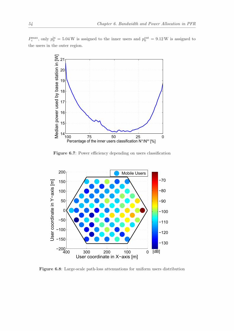
54 Chapter 6. Bandwidth and Power Allocation in PFR
Pmaxc , only pin0 = 5.04W is assigned to the inner users and pout0 = 9.12W is assigned to
the users in the outer region.
100 75 50 25 014
15
16
17
18
19
20
21
Percentage of the inner users classification N in/Ntot [%]
Media
n p
ow
er
used b
y b
ase s
tation in [W
]
Figure 6.7: Power efficiency depending on users classification
0100200300400−200
−150
−100
−50
0
50
100
150
200
User coordinate in X−axis [m]
User
coord
inate
in Y
−axis
[m
]
−130
−120
−110
−100
−90
−80
−70
Mobile Users
[dB]
Figure 6.8: Large-scale path-loss attenuations for uniform users distribution
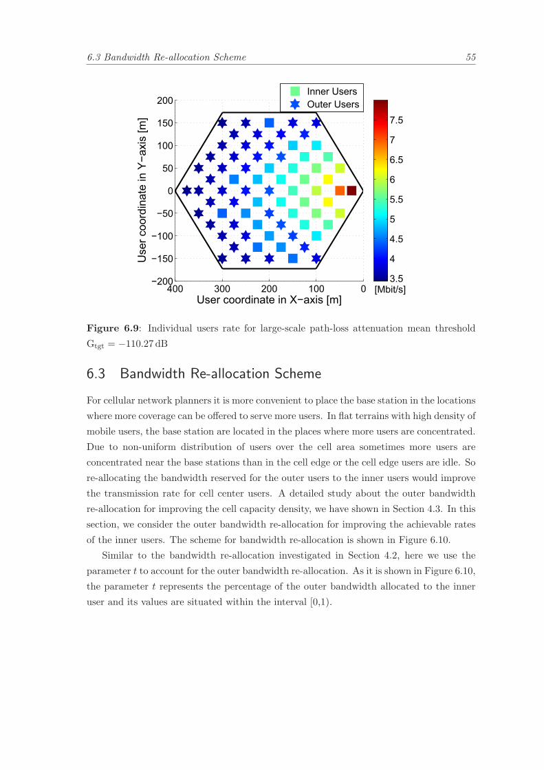
6.3 Bandwidth Re-allocation Scheme 55
0100200300400−200
−150
−100
−50
0
50
100
150
200
User coordinate in X−axis [m]
User
coord
inate
in Y
−axis
[m
]
3.5
4
4.5
5
5.5
6
6.5
7
7.5
Inner Users
Outer Users
[Mbit/s]
Figure 6.9: Individual users rate for large-scale path-loss attenuation mean threshold
Gtgt = −110.27 dB
6.3 Bandwidth Re-allocation Scheme
For cellular network planners it is more convenient to place the base station in the locations
where more coverage can be offered to serve more users. In flat terrains with high density of
mobile users, the base station are located in the places where more users are concentrated.
Due to non-uniform distribution of users over the cell area sometimes more users are
concentrated near the base stations than in the cell edge or the cell edge users are idle. So
re-allocating the bandwidth reserved for the outer users to the inner users would improve
the transmission rate for cell center users. A detailed study about the outer bandwidth
re-allocation for improving the cell capacity density, we have shown in Section 4.3. In this
section, we consider the outer bandwidth re-allocation for improving the achievable rates
of the inner users. The scheme for bandwidth re-allocation is shown in Figure 6.10.
Similar to the bandwidth re-allocation investigated in Section 4.2, here we use the
parameter t to account for the outer bandwidth re-allocation. As it is shown in Figure 6.10,
the parameter t represents the percentage of the outer bandwidth allocated to the inner
user and its values are situated within the interval [0,1).
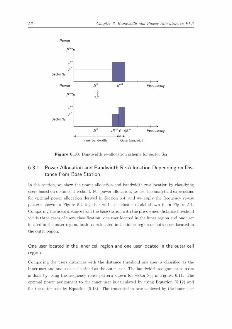
56 Chapter 6. Bandwidth and Power Allocation in PFR
inp
outp
inB
outB Frequency
Power
maxP
Sector S01
inp
outp
inB out)1( Bt- Frequency
Power
maxP
Sector S01
outtB
Inner bandwidth Outer bandwidth
Figure 6.10: Bandwidth re-allocation scheme for sector S01
6.3.1 Power Allocation and Bandwidth Re-Allocation Depending on Dis-tance from Base Station
In this section, we show the power allocation and bandwidth re-allocation by classifying
users based on distance threshold. For power allocation, we use the analytical expressions
for optimal power allocation derived in Section 5.4, and we apply the frequency re-use
pattern shown in Figure 5.4 together with cell cluster model shown in in Figure 5.1.
Comparing the users distance from the base station with the pre-defined distance threshold
yields three cases of users classification: one user located in the inner region and one user
located in the outer region, both users located in the inner region or both users located in
the outer region.
One user located in the inner cell region and one user located in the outer cell
region
Comparing the users distances with the distance threshold one user is classified as the
inner user and one user is classified as the outer user. The bandwidth assignment to users
is done by using the frequency reuse pattern shown for sector S01 in Figure. 6.11. The
optimal power assignment to the inner user is calculated by using Equation (5.12) and
for the outer user by Equation (5.13). The transmission rate achieved by the inner user
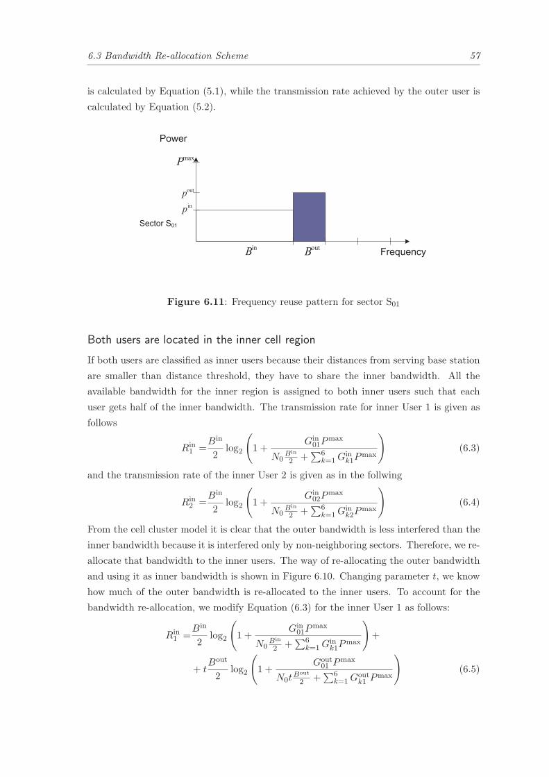
6.3 Bandwidth Re-allocation Scheme 57
is calculated by Equation (5.1), while the transmission rate achieved by the outer user is
calculated by Equation (5.2).
inp
outp
inB
outB Frequency
Power
maxP
Sector S01
Figure 6.11: Frequency reuse pattern for sector S01
Both users are located in the inner cell region
If both users are classified as inner users because their distances from serving base station
are smaller than distance threshold, they have to share the inner bandwidth. All the
available bandwidth for the inner region is assigned to both inner users such that each
user gets half of the inner bandwidth. The transmission rate for inner User 1 is given as
follows
Rin1 =
Bin
2log2
(
1 +Gin
01Pmax
N0Bin
2 +∑6
k=1Gink1P
max
)
(6.3)
and the transmission rate of the inner User 2 is given as in the follwing
Rin2 =
Bin
2log2
(
1 +Gin
02Pmax
N0Bin
2 +∑6
k=1Gink2P
max
)
(6.4)
From the cell cluster model it is clear that the outer bandwidth is less interfered than the
inner bandwidth because it is interfered only by non-neighboring sectors. Therefore, we re-
allocate that bandwidth to the inner users. The way of re-allocating the outer bandwidth
and using it as inner bandwidth is shown in Figure 6.10. Changing parameter t, we know
how much of the outer bandwidth is re-allocated to the inner users. To account for the
bandwidth re-allocation, we modify Equation (6.3) for the inner User 1 as follows:
Rin1 =
Bin
2log2
(
1 +Gin
01Pmax
N0Bin
2 +∑6
k=1Gink1P
max
)
+
+ tBout
2log2
(
1 +Gout
01 Pmax
N0tBout
2 +∑6
k=1Goutk1 Pmax
)
(6.5)

58 Chapter 6. Bandwidth and Power Allocation in PFR
Equation (6.4) for the rate of the inner User 2 is modified accordingly:
Rin2 =
Bin
2log2
(
1 +Gin
02Pmax
N0Bin
2 +∑6
k=1Gink2P
max
)
+
+ tBout
2log2
(
1 +Gout
02 Pmax
N0tBout
2 +∑6
k=1Gink2P
max
)
(6.6)
Both users located in the outer cell region
If both users are classified as outer users because their distances from the serving base
station are larger than distance threshold, they have to share the outer bandwidth from
the sector to which they belong. In this case, the inner bandwidth is not used due to the
possibility of experiencing high interference at the cell edge. So the transmission rate of
the first outer user is given by following equation
Rout1 =
Bout
2log2
(
1 +Gout
01 Pmax
N0Bout
2 +∑6
k=1Goutk1 Pmax
)
(6.7)
The Equation for the transmission rate of the outer User 2 is defined as in the following
Rout2 =
Bout
2log2
(
1 +Gout
02 Pmax
N0Bout
2 +∑6
k=1Goutk2 Pmax
)
(6.8)
In this case the outer users are very limited in bandwidth resources due to fixed bandwidth
allocation scheme.
Numerical Simulations: Power allocation and bandwidth re-allocation depend-
ing on distance from base station
In this section we consider uniform realization of users positions. A realistic urban scenario
is considered with its parameters shown in Table 6.3.
Table 6.3: Simulation parameters
parameters value
Maximum base station power Pmax 5 W
Maximum base station bandwidth Bmax 20 MHz
Noise spectral density N0 −174 dBm/Hz
Center frequency f 2.0 GHz
Pathloss exponent α 3.75
Penetration loss Lp 20 dB
Shadowing Xσ N (0, 8)dB
Small-scale Fading F χ22 dB,
Inter base station distance d 700 m
Number of user positions 100

6.3 Bandwidth Re-allocation Scheme 59
Using the simulation parameters shown in Table 6.3 and solution for optimal power
allocation taken out from optimization problem (5.5), we have shown the simulation results
for two users in Figure 6.12 in terms of maximum average sum-rate depending on users
random locations. We used the bandwidth reallocation scheme presented in Figure 6.10
depending on the user positions. For each specific realization of user positions we have
simulated 1000 channel realizations. For the specific simulation setup considered, the case
that both users are located in the inner region occurs with a probability of 59%. The case
when one user is located in the inner region and the other one located in the outer region
occurs with a probability of 35%. The last case when both users are located in the outer
region occurs with a probability of 6%.
From the simulation results shown in Figure 6.12 we see that the highest performance
is achieved when we consider the bandwidth re-allocation to the inner users. The lowest
performance is achieved when both users are located in the outer region since they are
located far from base stations, and they have to share a smaller portion of bandwidth
compared with the inner users. Without considering the re-allocation of the outer band-
width to the inner users, the best performance is achieved by optimal power assignment
when one user is located in the inner region and one user is located in the outer region.
0 1 2 3 4 50
10
20
30
40
50
60
Maximum base station power [W]
Ave
rag
e s
um
−ra
te f
or
ran
do
m u
se
r’s p
ositio
ns
in c
ert
ain
re
gio
n [
Mb
it/s
]
two inner users with bandwidth re−allocation t=99 %
one inner user and one outer user
two inner users without bandwidth re−allocation
two outer users
Figure 6.12: Maximum sum-rate for random users positions
In Figure 6.13 we show the simulation results for average sum-rate taken over random
users positions in the inner and outer regions. The lower curve represents the average of
all sum-rates when no re-allocation of the outer bandwidth to the inner users is carried
out. A better performance in terms of average sum-rate is achieved when we consider the

60 Chapter 6. Bandwidth and Power Allocation in PFR
re-allocation of the outer bandwidth to the inner user. This is shown by the upper curve
in Figure 6.13. A performance increase of approximately 34% is achieved.
0 1 2 3 4 50
10
20
30
40
50
60
Maximum base station power [W]
Ave
rag
e s
um
−ra
te f
or
ran
do
m u
se
r’s p
ositio
ns [
Mb
it/s
]
average sum−rate with bandwidth re−allocation
average sum−rate without bandwidth re−allocation
34%
Figure 6.13: Maximum average sum-rate for random users positions
6.3.2 Power Allocation and Bandwidth Re-allocation Depending on Large-scale Path-loss Attenuations
In this subsection, differently from Subsection 6.3.1, we show the power allocation and the
bandwidth re-allocation depending on mean LSPLA threshold. By comparing the LSPLA
of the users with the mean LSPLA threshold denoted by Gtgt, for two users located in
one cell, we have three cases of classifying the users. Based on the users classification, we
allocate the bandwidth and power to them.
One user located in the inner cell region and one user located in the outer cell
region
If the users LSPLA is higher than Gtgt, than that user is considered to be an inner user,
otherwise an outer user. While during comparing the users LSPLA with Gtgt threshold
we find that one user is classified to be the inner user and the other user to be the outer
user, in a such case the amount of bandwidth assigned to them is based on the frequency
reuse pattern shown for sector S01 in Figure 6.11. The optimal power assignment to the
inner is calculated using the analytical expression given by Equation (5.12). Similarly, we
calculate the power allocation to the outer user using Equation (5.13). The transmission

6.3 Bandwidth Re-allocation Scheme 61
rate achieved by the inner user, we calculate by using Equation (5.1), and the transmission
rate achieved by the outer user by Equation (5.2)
Both users are located in the inner cell region
If the LSPLA of both considered users are higher than Gtgt, in such case both users are
considered to be the inner users. Since, we have classified only inner users, they have
to share the inner bandwidth. The maximum base station power is assigned to both
inner users. The transmission rate for User 1 is calculated using Equation (6.3) and
similarly we calculate the transmission rate for the inner User 2 using Equation (6.4). The
LSPLA of direct channels Gin01, G
in02 are defined by Equation (5.3). The LSPLA of the
interference channels Gink1, G
ink2 are defined also by Equation (5.3) with F = 0dB. As we
have mentioned previously the outer bandwidth is less interfered than the inner bandwidth
since it is interfered only by non-neighboring sectors. We therefore re-allocate the outer
bandwidth to the inner users. The way of re-allocating the outer bandwidth and using it
as inner bandwidth is shown in the bandwidth re-allocation by Figure 6.10. To account
for the bandwidth re-allocation while calculating the transmission rate of the inner User
1, we use Equation (6.3). Similarly to the inner User 1, we use Equation (6.4) to account
for the bandwidth re-allocation during calculating the transmission rate.
Both users located in the outer cell region
Both users are considered as outer users if their LSPLA is lower than threshold Gtgt. In
this case, the inner bandwidth is not used at all due to the increase of ICI, since such
bandwidth experiences high interference at the cell edge. After we have only outer users,
the outer bandwidth is shared among them while the whole base station transmit power is
assigned to them. The LSPLA of direct channels Gout01 , Gout
02 are defined by Equation (5.3).
The LSPLA of interference channels Goutk1 , Gout
k2 are defined also by Equation (5.3). The
transmission rate of the outer User 1 is calculated using Equation (6.7) and similarly the
transmission rate for the outer User 2 is calculated using Equation (6.8).
Numerical Simulations: Power allocation and bandwidth re-allocation depend-
ing on LSPLA
In this simulation we consider uniform users positions. A realistic urban scenario is consid-
ered with its parameters shown in Table 6.4. The LSPLA results for two users depending
on the distance of each user to the base station are shown in Figure 6.14. To show the
values of LSPLA depending on the random distances of users from the base station, we
used the Equation (5.3) and the simulation parameters shown in Table 6.4. For simula-
tion setup, we have considered 100 uniform user positions, where per each position users
have experienced different channels. For each specific channel realization of random user

62 Chapter 6. Bandwidth and Power Allocation in PFR
positions, we have compared the LSPLA of users with the mean threshold Gtgt, and based
on that we have decided for users power allocation and bandwidth allocation. During
simulations we have noticed that the case that both users are located in the inner region
occurs with a probability of 16%. The case when one user is located in the inner region
and the other one located in the outer region occurs with a probability of 48%. The last
case when both users are located in the outer region occurs with a probability of 36%.
From the simulation results shown in Figure 6.14 we see that because of small-scale fading
and shadowing, sometimes the user which is located far from the base station has a better
LSPLA (better channel) than a user which is located near the base station. By classifying
the users as inner user and outer user depending on the LSPLA threshold, we are able to
assign the power and bandwidth resources in the optimal way, incease the sum-rate gain
and decrease the inter-cell interference.
Table 6.4: Simulation parameters
parameters value
Maximum base station power Pmax 5W
Maximum base station bandwidth Bmax 20MHz
Noise spectral density N0 −174 dBm/Hz
Center frequency f 2.0GHz
Pathloss exponent α 3.75
Penetration loss Lp 20 dB
Shadowing Xσ N (0, 8) dB
Small-scale Fading F χ22 dB,
Inter base station distance d 700m
Maximum cell range r (2/3)dm
Large-scale path-loss threshold Gtgt −106.4 dB,Number of channel realizations 100
Number of uniform users positions 100
In Figure 6.15, the sum-rate gain for dynamic method (classification of users is based
on distance threshold) compared with a static method (classification of users is based on
LSPLA threshold) is shown. For our simulation setup the static method defines a user as
inner user if its distance from its serving base station is in the range 0 < rin0 ≤ 0.70 · r.Analogously an outer user has a distance in the range 0.70 · r < rout0 ≤ r. Looking at
the simulation results shown in Figure 6.15, one can see that in some cases the dynamic
method outperforms the static method (the sum-rate gain is positive), while in some
cases both methods perform similar (the sum-rate gain is zero). This happens because
the dynamic method classifies a user with bad channel to be as outer user such that
experience less ICI, while the static method, for the same user with the same channel
classifies as inner user because the distance criteria. In this case the user classification by

6.3 Bandwidth Re-allocation Scheme 63
static method experience higher ICI. In all other cases when those methods perform the
same, means that they have done the same user classification. For all distance thresholds
from 0.70 · r to r, the dynamic method outperforms the static method at all positions.
0 20 40 60 80 1000
100
200
300
400
500D
ista
nce
of
the
use
rs f
rom
ba
se
sta
tio
ns [
m]
Number of channel realizations
−140
−120
−100
−80
−60
−40
−20User 1
User 2
dB
Figure 6.14: Large-scale path-loss attenuations for uniform users positions
0 10 20 30 40 50 60 70 80 90 1000
10
20
30
40
50
60
70
80
Number of channel realizations
Dyn
am
ic s
um
−ra
te g
ain
[%
]
Figure 6.15: Sum-rate gain for dynamic method compared with static method

64 Chapter 6. Bandwidth and Power Allocation in PFR
In Figure 6.16, the simulation results for average sum-rate taken over uniform users
positions in the inner and outer regions versus maximum base station power are shown.
The lower curve represents the average of all sum-rates when no re-allocation of the outer
bandwidth to the inner users is carried out for the static method used. A better perfor-
mance in terms of average sum-rate is achieved by the dynamic method. It is shown by
simulation results that a performance increase of approximately 16.4Mbit/s is achieved
by deploying the dynamic method. Considering also outer bandwidth re-allocation to the
inner users a performance increase of 3.1Mbit/s of the dynamic method compared to the
static method is achieved.
0 1 2 3 4 50
10
20
30
40
50
60
Maximum base station power [W]
Avera
ge s
um
−ra
te o
ver
channel re
alis
ations [M
bit/s
]
Dynamic with outer bandwidth re−allocation
Static with outer bandwidth re−allocation
Dynamic without outer bandwidth re−allocation
Static without outer bandwidth re−allocation
16.4 [Mbit/s]
3.1 [Mbit/s]
Figure 6.16: Maximum average sum-rate for uniform users positions
6.4 Power Allocation and Bandwidth Adaptation Algorithms
In this Section, we consider two optimization algorithms which are formulated for PFR:
the optimal power and adaptive bandwidth allocation, and the efficient power and adap-
tive bandwidth allocation. Th optimal power and adaptive bandwidth allocation algorithm
works in the principle of allocating the bandwidth to the users based on their classification
by the mean LSPLA threshold, while the power is allocated optimally in the cell regions.
The efficient power and adaptive bandwidth allocation algorithm works in the same prin-
ciple for power allocation as previous algorithm, while the power is allocated to the cell
regions efficiently.
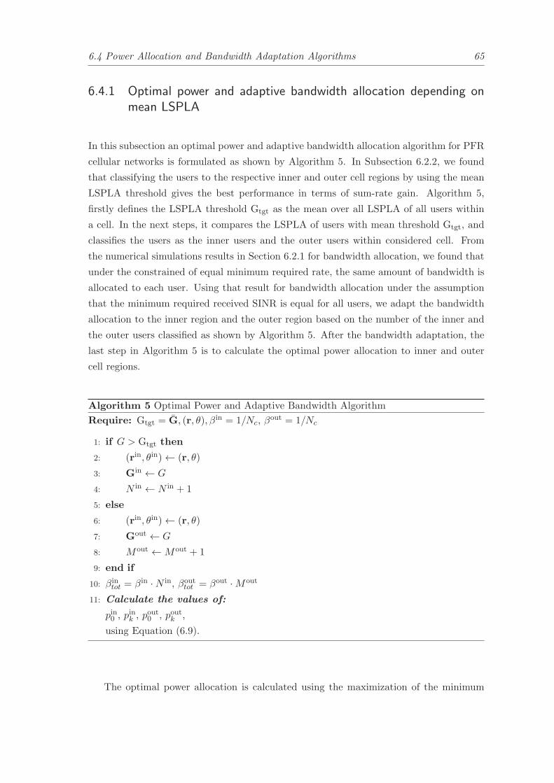
6.4 Power Allocation and Bandwidth Adaptation Algorithms 65
6.4.1 Optimal power and adaptive bandwidth allocation depending onmean LSPLA
In this subsection an optimal power and adaptive bandwidth allocation algorithm for PFR
cellular networks is formulated as shown by Algorithm 5. In Subsection 6.2.2, we found
that classifying the users to the respective inner and outer cell regions by using the mean
LSPLA threshold gives the best performance in terms of sum-rate gain. Algorithm 5,
firstly defines the LSPLA threshold Gtgt as the mean over all LSPLA of all users within
a cell. In the next steps, it compares the LSPLA of users with mean threshold Gtgt, and
classifies the users as the inner users and the outer users within considered cell. From
the numerical simulations results in Section 6.2.1 for bandwidth allocation, we found that
under the constrained of equal minimum required rate, the same amount of bandwidth is
allocated to each user. Using that result for bandwidth allocation under the assumption
that the minimum required received SINR is equal for all users, we adapt the bandwidth
allocation to the inner region and the outer region based on the number of the inner and
the outer users classified as shown by Algorithm 5. After the bandwidth adaptation, the
last step in Algorithm 5 is to calculate the optimal power allocation to inner and outer
cell regions.
Algorithm 5 Optimal Power and Adaptive Bandwidth Algorithm
Require: Gtgt = G, (r, θ),βin = 1/Nc, βout = 1/Nc
1: if G > Gtgt then
2: (rin, θin)← (r, θ)
3: Gin ← G
4: N in ← N in + 1
5: else
6: (rin, θin)← (r, θ)
7: Gout ← G
8: Mout ←Mout + 1
9: end if
10: βintot = βin ·N in, βout
tot = βout ·Mout
11: Calculate the values of:
pin0 , pink , p
out0 , poutk ,
using Equation (6.9).
The optimal power allocation is calculated using the maximization of the minimum
66 Chapter 6. Bandwidth and Power Allocation in PFR
SINR formulated by Equation (6.9) under sum-power constraints.
maximizeβincn,β
outcm∈R+,p�0
min{SINRinc1, ..., SINR
incNin , SINR
outc1 , ..., SINRout
cMout} (6.9a)
subject to
pinc + poutc ≤ Pmaxc , ∀c ∈ C, (6.9b)
The bandwidth adaptation carried out by Algorithm 5 has result in a simplified opti-
mization problem given by Equation (6.9), since it contains only the sum-power constraints
(6.9b). The maximization of the minimum SINR formulated by Equation (6.9) is a GGP
optimization problem that maximizes the minimum SINR constrained by optimal power
allocation in PFR. Finding the direct solution is not easy due to formulation of the prob-
lem in GGP form. Similarly to the previous problems in GGP form, without making any
assumption on high-SINR approximation [14], we convert the formulated optimization
problem (6.9) into a GP optimization problem and solve it efficiently using CVX. The
SINR in the general form for user s within cell c is given by the following equation:
SINRIcs =
pIcnins β
incs +
∑
k∈C\c ginksp
ink
. (6.10)
In Equation (6.10), the superscript I ∈ {in, out} denotes the superscript for the inner
users or superscript for the outer users. Further, the subscript s ∈ {n,m} denotes the
indexes for inner user n or the outer user m.
Proposition 4. The maximization of the minimum SINR formulated by Equation ( 6.9)
can be transformed into GP optimization problem.
Proof. Similarly to the transformation of the maximization of the minimum rate shown in
Subsection 6.2.1, by introducing the auxiliary variable z such that received SINRs by users
is lower bounded by z, the functions in the objective are converted into SINR constraints.
Since the left side of those constraints are not posynomilas, the inversion of nominator
with the denominator in both sides of the SINR constrains is used to convert them into
posynomials. The power constraint remains the same since they are posynomials. So the
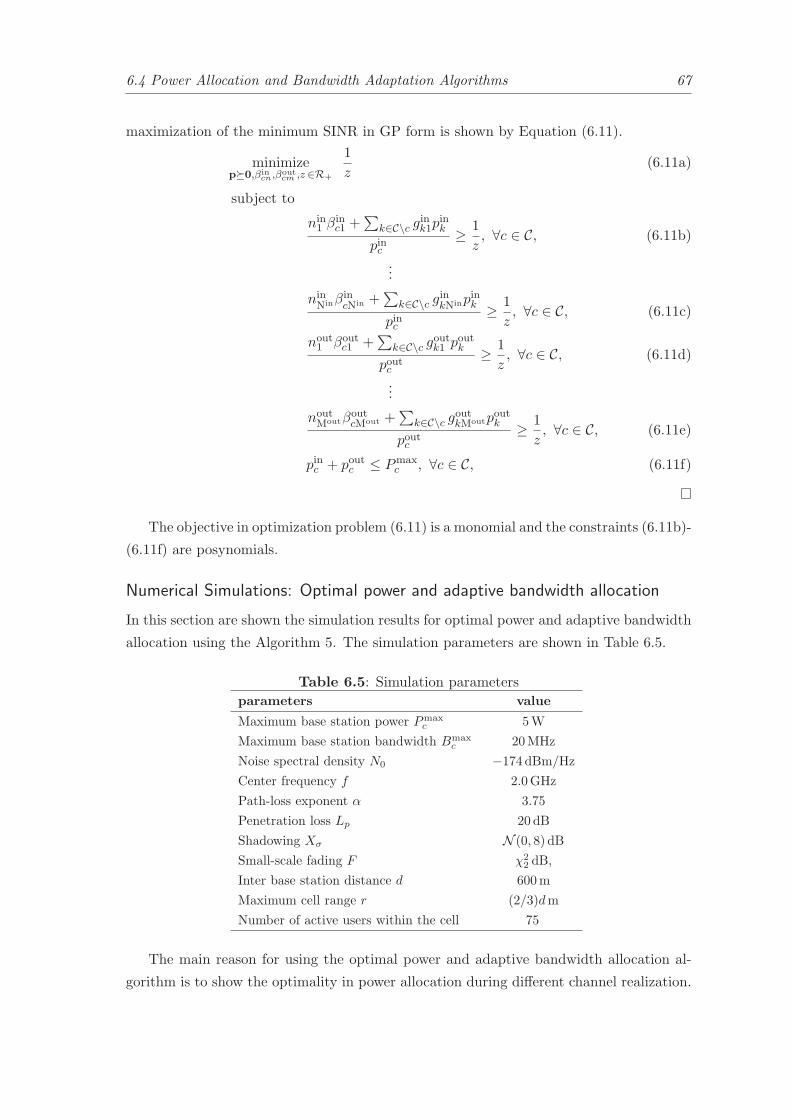
6.4 Power Allocation and Bandwidth Adaptation Algorithms 67
maximization of the minimum SINR in GP form is shown by Equation (6.11).
minimizep�0,βin
cn,βoutcm ,z ∈R+
1
z(6.11a)
subject to
nin1 β
inc1 +
∑
k∈C\c gink1p
ink
pinc≥ 1
z, ∀c ∈ C, (6.11b)
...
ninNinβ
incNin +
∑
k∈C\c ginkNinp
ink
pinc≥ 1
z, ∀c ∈ C, (6.11c)
nout1 βout
c1 +∑
k∈C\c goutk1 poutk
poutc
≥ 1
z, ∀c ∈ C, (6.11d)
...
noutMoutβout
cMout +∑
k∈C\c goutkMoutpoutk
poutc
≥ 1
z, ∀c ∈ C, (6.11e)
pinc + poutc ≤ Pmaxc , ∀c ∈ C, (6.11f)
The objective in optimization problem (6.11) is a monomial and the constraints (6.11b)-
(6.11f) are posynomials.
Numerical Simulations: Optimal power and adaptive bandwidth allocation
In this section are shown the simulation results for optimal power and adaptive bandwidth
allocation using the Algorithm 5. The simulation parameters are shown in Table 6.5.
Table 6.5: Simulation parameters
parameters value
Maximum base station power Pmaxc 5W
Maximum base station bandwidth Bmaxc 20MHz
Noise spectral density N0 −174 dBm/Hz
Center frequency f 2.0GHz
Path-loss exponent α 3.75
Penetration loss Lp 20 dB
Shadowing Xσ N (0, 8) dB
Small-scale fading F χ22 dB,
Inter base station distance d 600m
Maximum cell range r (2/3)dm
Number of active users within the cell 75
The main reason for using the optimal power and adaptive bandwidth allocation al-
gorithm is to show the optimality in power allocation during different channel realization.

68 Chapter 6. Bandwidth and Power Allocation in PFR
In the following we show the power allocation to the inner users and to the outer users
only for the first 10 realizations. The optimal power allocation to the inner users for the
first 10 realization versus the maximum base station power is shown in Figure 6.17. From
the simulation results shown in Figure 6.17 one can see that at the first realization most of
the maximum transmit base station power Pmax = 5W is allocated to the inner users. To
understand the reason for such a power allocation, in the following we show the simulation
results for the LSPLA and the achievable rate. The LSPLA during realization 1 for the
users located uniformly over the distance within cell area is shown in Figure 6.18. Using
the mean LSPLA as threshold Gtgt = −108.96 for realization 1, Algorithm 5 has classified
around 33 users as inner users and around 42 users as outer users. The user classification
and their achievable rates for the maximum base station power Pmax = 5W is shown in
Figure 6.19. In the simulation results, shown in Figure 6.19 it can be observed that each
inner and the outer user has achieved a rate higher than 2.5Mbit/s.
Figure 6.17: Optimal power allocation to the inner users

6.4 Power Allocation and Bandwidth Adaptation Algorithms 69
For the same realization of 10 channels, Figure 6.20 shows the optimal power alloca-
tion to the outer users. Analyzing the simulation results presented in Figure 6.20 one
can see that from the first 10 realizations in the realization 3 most of the transmit base
station power Pmax = 5W is allocated to the outer users. To see the effects of such
power allocation for realization 3, we analyze the LSPLA and the achievable rate for the
realization 3. The LSPLA of users for realization 3 is shown in Figure 6.21. Using the
mean LSPLA threshold Gtgt = −110.70 dB for the maximum base station transmit power
Pmax = 5W, Figure 6.22 shows the user classification as the inner and the outer users and
their achievable rates. From the simulation results shown in Figure 6.22 it has been found
that around 31 users are classified as inner users and around 44 users are classified as
outer users. Even most of the power has been allocated to the outer users for realization
3, still each inner and outer user has achieved a rate higher that 2.5Mbit/s.
0100200300400
−200
−150
−100
−50
0
50
100
150
200
User coordinate in X−axis [m]
User
coord
inate
in Y
−axis
[m
]
−130
−120
−110
−100
−90
[dB]
Figure 6.18: Large-scale path-loss attenuations for the realization 1
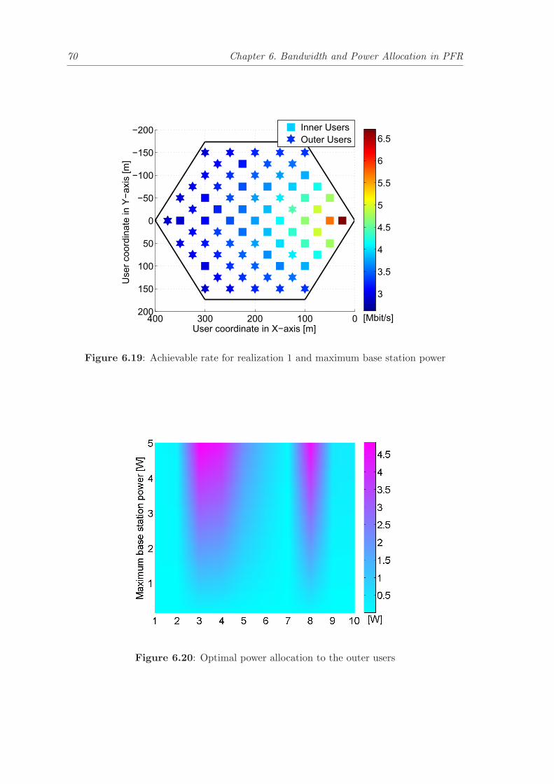
70 Chapter 6. Bandwidth and Power Allocation in PFR
0100200300400
−200
−150
−100
−50
0
50
100
150
200
User
coord
inate
in Y
−axis
[m
]
User coordinate in X−axis [m]
3
3.5
4
4.5
5
5.5
6
6.5
Inner Users
Outer Users
[Mbit/s]
Figure 6.19: Achievable rate for realization 1 and maximum base station power
Figure 6.20: Optimal power allocation to the outer users

6.4 Power Allocation and Bandwidth Adaptation Algorithms 71
0100200300400
−200
−150
−100
−50
0
50
100
150
200
User coordinate in X−axis [m]
User
coord
inate
in Y
−axis
[m
]
−130
−120
−110
−100
−90
−80
[dB]
Figure 6.21: Large-scale path-loss attenuations for the realization 3
0100200300400
−200
−150
−100
−50
0
50
100
150
200
User coordinate in X−axis [m]
User
coord
inate
in Y
−axis
[m
]
3
3.5
4
4.5
5
5.5
6
6.5Inner Users
Outer Users
[Mbit/s]
Figure 6.22: Achievable rate for realization 3 and maximum base station power
72 Chapter 6. Bandwidth and Power Allocation in PFR
6.4.2 Efficient power and adaptive bandwidth algorithm depending onmean LSPLA
In this subsection, we show the formulation of the efficient power allocation and adaptive
bandwidth allocation algorithm similar to Algorithm 5 for PFR cellular networks.
Algorithm 6 Efficient Power and Adaptive Bandwidth Algorithm
Require: Gtgt = G, (r, θ),βin = 1/Nc, βout = 1/Nc
1: if G > Gtgt then
2: (rin, θin)← (r, θ)
3: Gin ← G
4: N in ← N in + 1
5: else
6: (rin, θin)← (r, θ)
7: Gout ← G
8: Mout ←Mout + 1
9: end if
10: βintot = βin ·N in, βout
tot = βout ·Mout
11: Calculate the values of:
pin0 , pink , p
out0 , poutk ,
using Equation (6.12).
The sum-power minimization problem is given by Equation (6.12).
minimizeβincn,β
outcm∈R+,p�0
Nin∑
n=1
pincn +
Mout∑
m=1
poutcm (6.12a)
subject to
pincnin1 β
inc1 +
∑
k∈C\c gink1p
ink
≥ SINRinmin, ∀c ∈ C, (6.12b)
...
pincninNinβ
incNin +
∑
k∈C\c ginkNinp
ink
≥ SINRinmin, ∀c ∈ C, (6.12c)
poutc
nout1 βout
c1 +∑
k∈C\c goutk1 poutk
≥ SINRoutmin, ∀c ∈ C, (6.12d)
...
poutc
noutMoutβout
cMout +∑
k∈C\c goutkMoutpoutk
≥ SINRoutmin, ∀c ∈ C, (6.12e)
pinc + poutc ≤ Pmaxc , ∀c ∈ C, (6.12f)
6.4 Power Allocation and Bandwidth Adaptation Algorithms 73
Algorithm 6 works in principle as the Algorithm 5, except that instead of maximizing
the minimum SINR deploys a sum-power minimization to efficiently allocate the power to
the inner and the outer users.
The objective (6.12a) minimizes all power in all regions of the considered cells. The
constraints (6.12b)-(6.12c) show that the individual inner users SINR’s are lower bounded
by the minimum inner user SINR. Similarly to the inner users, the constraints (6.12d)-
(6.12e) show that the SINRs for outer users are lower bounded by the minimum outer
user SINR. The last constraint (6.13f) shows that the sum of power allocated in the inner
region and the outer region should not be higher than the maximum base station power.
As it is formulated the optimization problem is not a GP or any other extended forms of
GP’s like GGP due to non-posynomial standard form of SINR constraints.
Proposition 5. The sum-power minimization problem ( 6.12) can be converted into a
geometric programming problem.
Proof. Similarly to the optimization problem given by Equation (6.9), we begin by chang-
ing the nominator with the denominator in the constraints (6.12b)-(6.12e) in order to
convert them to posynomials. This led us to the optimization problem formulated in the
GP form as formulated in the following
minimizeβincn,β
outcm∈R+,p�0
Nin∑
n=1
pincn +Mout∑
m=1
poutcm (6.13a)
subject to
nin1 β
inc1 +
∑
k∈C\c gink1p
ink
pinc≤ 1
SINRinmin
, ∀c ∈ C, (6.13b)
...
ninNinβ
incNin +
∑
k∈C\c ginkNinp
ink
pinc≤ 1
SINRinmin
, ∀c ∈ C, (6.13c)
nout1 βout
c1 +∑
k∈C\c goutk1 poutk
poutc
≤ 1
SINRoutmin
, ∀c ∈ C, (6.13d)
...
noutMoutβout
cMout +∑
k∈C\c goutkMoutpoutk
poutc
≤ 1
SINRoutmin
, ∀c ∈ C, (6.13e)
pinc + poutc ≤ Pmaxc , ∀c ∈ C, (6.13f)
where the objective (6.13a) and the constraints (6.13b)-(6.13f) are posynomials.
Numerical Simulations: Efficient power and adaptive bandwidth allocation
The simulation results shown here are carried out using Algorithm 6 and the simulation
parameters in Table 6.6.

74 Chapter 6. Bandwidth and Power Allocation in PFR
Table 6.6: Simulation parameters
parameters value
Maximum base station power Pmaxc 40W
Maximum base station bandwidth Bmaxc 20MHz
Noise spectral density N0 −174 dBm/Hz
Center frequency f 2.0GHz
Path-loss exponent α 3.75
Penetration loss Lp 20 dB
Shadowing Xσ N (0, 8) dB
Small-scale fading F χ22 dB,
Inter base station distance d 600m
Maximum cell range r (2/3)dm
Users requirement SINR SINRmin [0 : 0.5 : 25] dB
Number of users within cell 75
During the simulations 100 realizations are considered, where for each realization the
users have experienced different channels. The average power allocation for the inner
region and the outer region versus the minimum required SINR is shown in Figure 6.23.
0 5 10 15 20 250
0.2
0.4
0.6
0.8
1
1.2
Minimum requirement SINR [dB]
Avera
ge p
ow
er
allo
cation [W
]
Outer Power Allocation
Inner Power Allocation
Figure 6.23: Average power allocation for the inner region and the outer region
The simulation results shown in Figure 6.23 indicate high efficiency of power allocation
performed by Algorithm 6, for low minimum required SINR. Increasing the minimum
SINR requirement, increases also the average power allocated to the inner and the outer
regions. Even for a SINR requirement of 25 dB the average power allocated in the inner
region is below 1W and that allocated to the outer region below 1.2W.
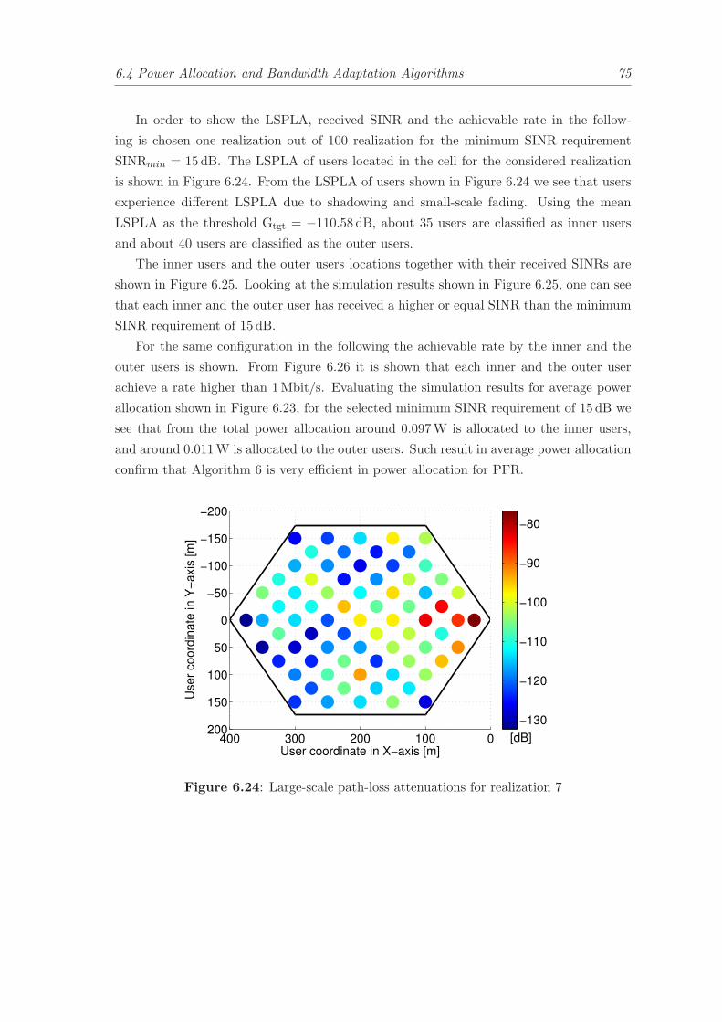
6.4 Power Allocation and Bandwidth Adaptation Algorithms 75
In order to show the LSPLA, received SINR and the achievable rate in the follow-
ing is chosen one realization out of 100 realization for the minimum SINR requirement
SINRmin = 15dB. The LSPLA of users located in the cell for the considered realization
is shown in Figure 6.24. From the LSPLA of users shown in Figure 6.24 we see that users
experience different LSPLA due to shadowing and small-scale fading. Using the mean
LSPLA as the threshold Gtgt = −110.58 dB, about 35 users are classified as inner users
and about 40 users are classified as the outer users.
The inner users and the outer users locations together with their received SINRs are
shown in Figure 6.25. Looking at the simulation results shown in Figure 6.25, one can see
that each inner and the outer user has received a higher or equal SINR than the minimum
SINR requirement of 15 dB.
For the same configuration in the following the achievable rate by the inner and the
outer users is shown. From Figure 6.26 it is shown that each inner and the outer user
achieve a rate higher than 1Mbit/s. Evaluating the simulation results for average power
allocation shown in Figure 6.23, for the selected minimum SINR requirement of 15 dB we
see that from the total power allocation around 0.097W is allocated to the inner users,
and around 0.011W is allocated to the outer users. Such result in average power allocation
confirm that Algorithm 6 is very efficient in power allocation for PFR.
0100200300400
−200
−150
−100
−50
0
50
100
150
200
User coordinate in X−axis [m]
User
coord
inate
in Y
−axis
[m
]
−130
−120
−110
−100
−90
−80
[dB]
Figure 6.24: Large-scale path-loss attenuations for realization 7

76 Chapter 6. Bandwidth and Power Allocation in PFR
0100200300400
−200
−150
−100
−50
0
50
100
150
200
User coordinate in X−axis [m]
User
coord
inate
in Y
−axis
[m
]
15
20
25
30
35
40
45
50
55
Inner Users
Outer Users
[dB]
Figure 6.25: Users received SINRs
0100200300400
−200
−150
−100
−50
0
50
100
150
200
User coordinate in X−axis [m]
User
coord
inate
in Y
−axis
[m
]
1.5
2
2.5
3
3.5
4
4.5
5
Inner Users
Outer Users
[Mbit/s]
Figure 6.26: Achievable rate by the users
7
Conclusions
IN the thesis I give an overview of the RRM techniques for PFR in LTE networks. The
3GPP, by whom LTE is standardized, proposes OFDMA as multiple access scheme in
the downlink. Due to the use of OFDMA the ICI becomes critical at the cell edge. One of
the many tasks of RRM is the reduction of the ICI while increasing the achievable capacity
of the network. Two radio resources are considered to be of primary importance: power
and bandwidth. Both radio resources are very limited and costly. The power is limited
due to the associated increase of the ICI to the neighboring cells, while the bandwidth
is limited due to limited spectrum license. Hence optimization of such resources is ad-
vantageous. We have formulated optimization problems for RRA which are efficient and
optimal in resource allocation. These problems are formulated based on the mathemat-
ical framework of convex optimization. The mathematical methods used throughout the
thesis are introduced in Chapter 3. The main part of the thesis is focused on three topics:
capacity density maximization, power allocation and joint power and bandwidth alloca-
tion. Initially, we considered the maximization of the cell capacity density by applying a
bandwidth re-allocation scheme with constant power allocation. Next, we developed op-
timization problems for power allocation. Finally, we developed optimization techniques
for joint power and bandwidth allocation. Overall, we formulated efficient, optimal power
allocation and adaptive bandwidth allocation algorithms.
In the following we present the most important conclusions for capacity density max-
imization, power allocation in PFR, as well as joint power and bandwidth allocation in
PFR.
77

78 Chapter 7. Conclusions
7.1 Capacity Density Maximization
We developed and analyzed a novel flexible bandwidth allocation scheme [7] for PFR
considering the case that the cell is not always populated homogeneously over the area.
We formulated the capacity density taking into account cell edge bandwidth re-allocation.
Further, we formulated the optimization problem for maximizing the capacity density
constrained by optimum frequency partitioning radius and the the cell edge bandwidth re-
allocation parameter. By solving the optimization problems for maximizing the capacity
density we found an upper bound on cell edge bandwidth re-allocation.
Simulations indicated that re-allocating the cell edge bandwidth to the cell center
increases the capacity density by 4.9 bit/s/Hz for frequency reuse-1 whenever the cell
edge users are idling.
7.2 Power Allocation in Partial Frequency Reuse
In this part of thesis, we introduced the cell cluster scheme for PFR where the user’s clas-
sification into cell regions is obtained based on the LSPLA threshold. We formulated the
optimization problems for sum-rate maximization [12] in PFR considering the bandwidth
and the power allocation. In general, such problems are non-convex and, therefore, hard
to solve. However, under the additional assumption of a uniform power allocation over all
cells, we are able to convexify this optimization problem.
Using dual decomposition techniques, we found the optimal power allocation in the
inner and the outer cell regions for a fixed bandwidth allocation within cell regions. Such
optimal allocation of power significantly reduces the ICI and simultaneously increases the
sum-rate.
Simulations showed also that our optimal power allocation algorithm outperforms the
static power allocation method. The gains achieved by our algorithm compared with static
power allocation are shown in the maximum sum-rate.
Moreover, we formulated the optimization problem for the maximization of the mini-
mum rate and for the minimization of the sum-power for multiple users over multiple cells
in PFR. A variable transformation was able to convert these non-convex optimization
problems into convex forms which are solvable efficiently using well known state-of-the-art
interior-point methods.
7.3 Bandwidth and Power Allocation in Partial Frequency Reuse
Finally, we optimized jointly the bandwidth and power allocation by solving the max-
imization of the minimum rate. We found efficient solutions for power allocation and

7.3 Bandwidth and Power Allocation in Partial Frequency Reuse 79
optimal solutions for bandwidth allocation. Also by analyzing the simulation results we
proved that PFR is more efficient in power allocation that frequency reuse-1 or frequency
reuse-3. Such efficiency is achieved when for user’s classification in cell regions the LSPLA
threshold is defined as the mean LSPLA.
Further, we treated the allocation of power and re-allocation of bandwidth jointly and
show that a significant increase in the sum-rate for the cell center users is achievable.
Firstly, the joint power allocation and bandwidth re-allocation algorithms are proposed
and applied to the cell cluster where we classify the users based on the distance threshold
(static method). Later we have applied the same optimization algorithm for a cell cluster
where the user’s classification is based on mean LSPLA threshold (dynamic method).
By simulation it is shown that about 34% more gain is achieved in average sum rate
when the bandwidth re-allocation is considered for the static method. Further we com-
pared the dynamic method with the static method where in most of the cases a higher
gain is achieved by dynamic method. There are only few cases when both methods per-
form similarly. Also in the case of average sum-rate we achieve a sum-rate increase by
3.1Mbit/s with the dynamic method compared to the static method when outer band-
width re-allocation is considered. About 16.4Mbit/s more sum-rate is achieved for the
same scenario without outer bandwidth re-allocation.
Concerning the bandwidth allocation by maximization of the minimum rate we have
noticed that bandwidth allocation in the cell regions is obtained depending on the amount
of the user’s classified. Using this fact, we have developed two algorithms: the optimal
power and adaptive bandwidth algorithm and the efficient power and adaptive bandwidth
algorithm.
The optimal power and adaptive bandwidth algorithm use the maximization of the
minimum SINR to optimally allocate the power in the cell regions, while the bandwidth
is allocated adaptively based on the user’s classification by LSPLA threshold. Applying
such algorithm is shown that each user has achieved a rate higher than 2.5Mbit/s for the
maximum base station transmit power 5W.
The efficient power and adaptive bandwidth allocation algorithm use the sum-power
minimization to efficiently allocate the power in the cell regions based on the minimum
received SINR criteria, while it allocates the bandwidth adaptively based on the user’s
classification by the LSPLA threshold. With such algorithm it is shown that each user
has achieved a SINR higher that minimum requirement SINR and a transmission rate
higher than 1.5Mbit/s even for an average power allocation smaller than 1.2W.


8Future Directions / Outlook
THE main contribution of this thesis is the development of optimization problems for
RRA in PFR cellular networks.
In the first part we introduced a novel bandwidth re-allocation scheme for PFR and
formulated the optimization problem that maximize the cell capacity density taking into
account bandwidth re-allocation. The results were quite impressive and confirmed the
gain from re-allocating the cell edge bandwidth to the cell center users when the cell edge
users are idle.
In the second part we formulated the RRA optimization problems for power alloca-
tion. We applied the DDT to solve such optimization problems for PFR. A significant
decrease in the ICI and a significant increase in the sum-rate is achieved. Such optimiza-
tion techniques are proved to work well for fixed bandwidth allocation schemes. However
for variable bandwidth allocation the dual decomposition methods offer intractable solu-
tions. Implementing a scheduler together with the optimization of the power allocation is
a future direction. Also using interior point algorithms based on barrier methods is the
next task to solve the joint optimization of power and bandwidth allocation in PFR.
In the third part which is the last part of the thesis we formulated the optimization
problems for joint optimization of power and bandwidth allocation applying GP. We
achieved very good results which could be interesting for cellular network operators on
how to dimension the cell. By dimensioning cells we mean that no matter where the
user is, either at the cell center or cell edge, it should be able to receive a rate higher
than a minimum required rate or an SINR higher than minimum required SINR. The
next step will be to compare the aforementioned optimization algorithms for PFR with
frequency reuse-1. Such results are expected to help the mobile operators to decide on
implementation the PFR in LTE networks.
81

82 Chapter 8. Future Directions / Outlook
From all what I showed in the thesis one can understand that there are still many
open questions for research in resource optimization for LTE. Finding solution for such
problems would yield in energy saving and simultaneously, offer higher data rates to the
users.
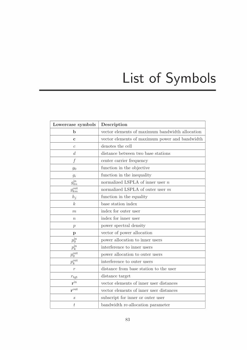
List of Symbols
Lowercase symbols Description
b vector elements of maximum bandwidth allocation
c vector elements of maximum power and bandwidth
c denotes the cell
d distance between two base stations
f center carrier frequency
g0 function in the objective
gi function in the inequality
ginkn normalized LSPLA of inner user n
goutkm normalized LSPLA of outer user m
hj function in the equality
k base station index
m index for outer user
n index for inner user
p power spectral density
p vector of power allocation
pin0 power allocation to inner users
pink interference to inner users
pout0 power allocation to outer users
poutk interference to outer users
r distance from base station to the user
rtgt distance target
rin vector elements of inner user distances
rout vector elements of inner user distances
s subscript for inner or outer user
t bandwidth re-allocation parameter
83

t∗ maximum bandwidth re-allocation
tin normalized required inner user rate
tin normalized required outer user rate
u user
v velocity of light in free space
x vector of optimization variables
x normalized cartesian coordinate of X
y normalized cartesian coordinate of Y
z auxiliary variable
Uppercase symbols Description
A normalization matrix
Ak sum of BS and MS antenna gain
Am antenna attenuation
A(θ) horizontal antenna pattern
Btot total base station bandwidth
BFR bandwidth assigned to FR region
BPR bandwidth assigned to PR region
Binn bandwidth assigned to to user n in inner region
Boutm bandwidth assigned to to user m in outer region
Bmax maximum base station bandwidth
C cell capacity density
CFR cell capacity density in FR region
CPR bandwidth assigned to PR region
C set of cells
F fast fading
G large-scale path-loss attenuation (LSPLA)
G objective of a dual optimization problem
Gin0n LSPLA of direct channels for inner user n
Ginkn LSPLA of interference channels for inner user n
Gout0m LSPLA of direct channels for outer user m
Goutkm LSPLA of interference channels for inner user m
Gin vector elements for LSPLA of inner users
Gout vector elements for LSPLA of outer users
I superscript for inner or outer set of users
L Lagrangian of an optimization problem
Lr FSPL model
84
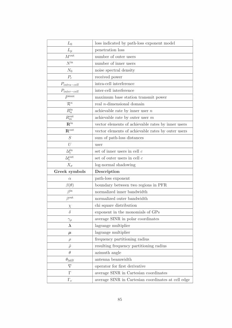
L0 loss indicated by path-loss exponent model
Lp penetration loss
Mout number of outer users
N in number of inner users
N0 noise spectral density
Pr received power
Pintra−cell intra-cell interference
Pinter−cell inter-cell interference
Pmax maximum base station transmit power
Rn real n-dimensional domain
Rinn achievable rate by inner user n
Routm achievable rate by outer user m
Rin vector elements of achievable rates by inner users
Rout vector elements of achievable rates by outer users
S sum of path-loss distances
U user
U inc set of inner users in cell c
Uoutc set of outer users in cell c
Xσ log-normal shadowing
Greek symbols Description
α path-loss exponent
β(θ) boundary between two regions in PFR
βin normalized inner bandwidth
βout normalized outer bandwidth
χ chi square distribution
δ exponent in the monomials of GPs
γρ average SINR in polar coordinates
λ lagrange multiplier
µ lagrange multiplier
ρ frequency partitioning radius
ρ resulting frequency partitioning radius
θ azimuth angle
θ3dB antenna beamwidth
∇ operator for first derivative
Γ average SINR in Cartesian coordinates
Γe average SINR in Cartesian coordinates at cell edge
85

86
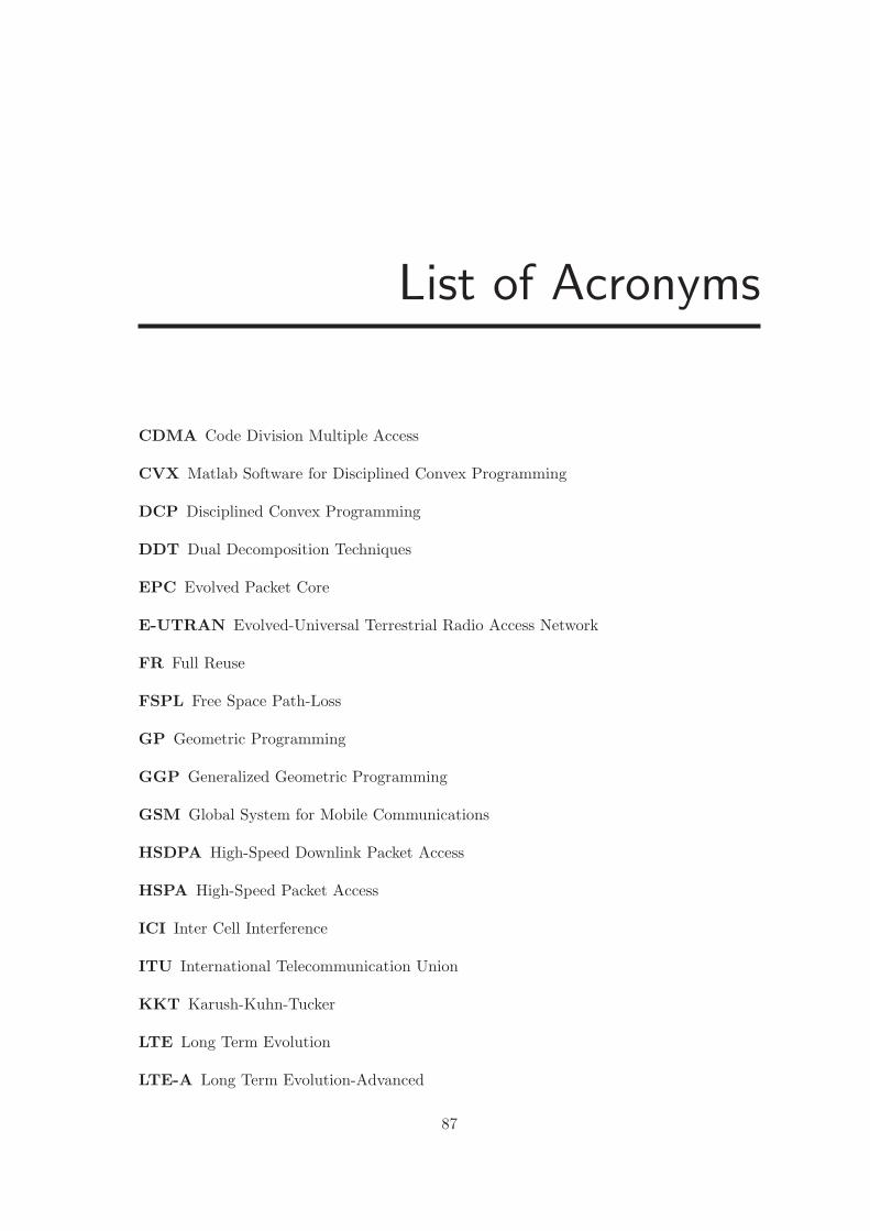
List of Acronyms
CDMA Code Division Multiple Access
CVX Matlab Software for Disciplined Convex Programming
DCP Disciplined Convex Programming
DDT Dual Decomposition Techniques
EPC Evolved Packet Core
E-UTRAN Evolved-Universal Terrestrial Radio Access Network
FR Full Reuse
FSPL Free Space Path-Loss
GP Geometric Programming
GGP Generalized Geometric Programming
GSM Global System for Mobile Communications
HSDPA High-Speed Downlink Packet Access
HSPA High-Speed Packet Access
ICI Inter Cell Interference
ITU International Telecommunication Union
KKT Karush-Kuhn-Tucker
LTE Long Term Evolution
LTE-A Long Term Evolution-Advanced
87
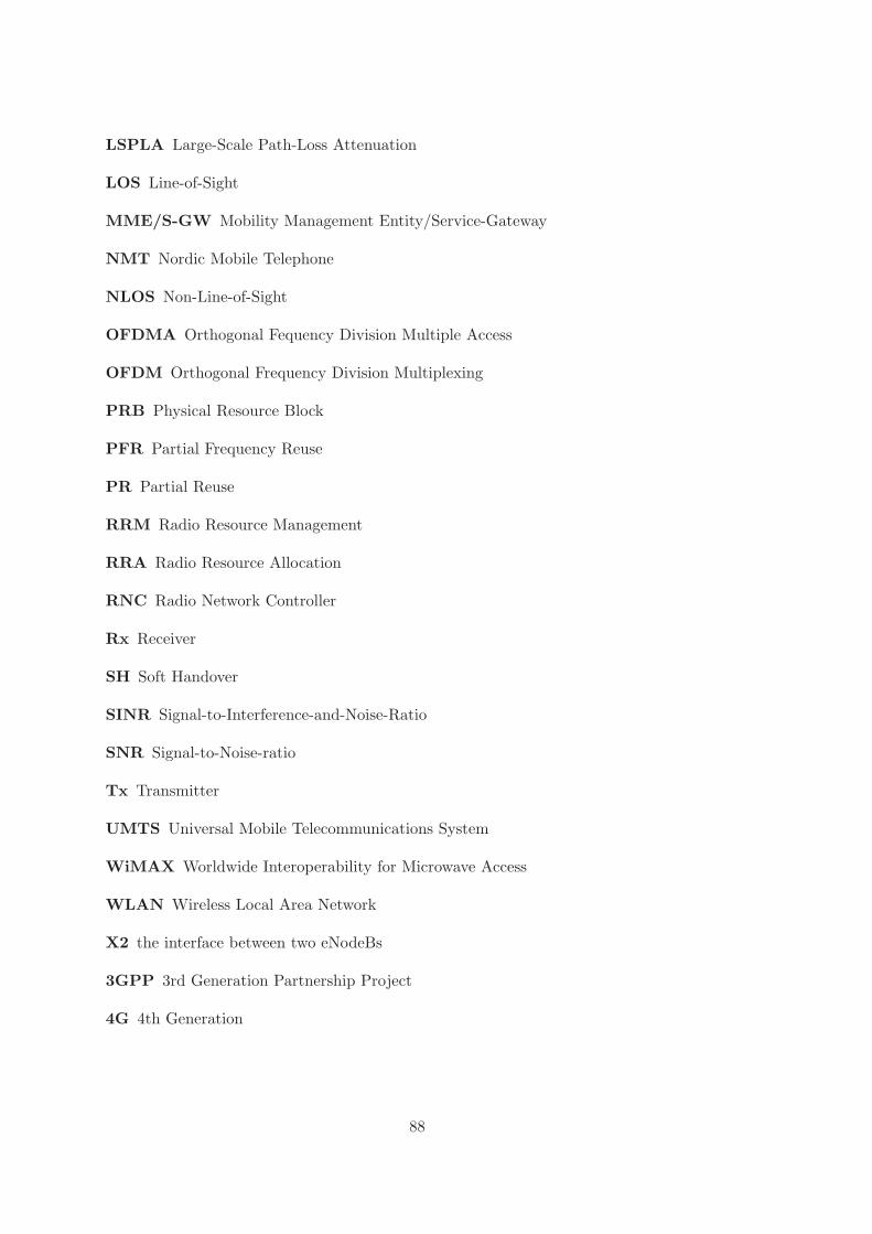
LSPLA Large-Scale Path-Loss Attenuation
LOS Line-of-Sight
MME/S-GW Mobility Management Entity/Service-Gateway
NMT Nordic Mobile Telephone
NLOS Non-Line-of-Sight
OFDMA Orthogonal Fequency Division Multiple Access
OFDM Orthogonal Frequency Division Multiplexing
PRB Physical Resource Block
PFR Partial Frequency Reuse
PR Partial Reuse
RRM Radio Resource Management
RRA Radio Resource Allocation
RNC Radio Network Controller
Rx Receiver
SH Soft Handover
SINR Signal-to-Interference-and-Noise-Ratio
SNR Signal-to-Noise-ratio
Tx Transmitter
UMTS Universal Mobile Telecommunications System
WiMAX Worldwide Interoperability for Microwave Access
WLAN Wireless Local Area Network
X2 the interface between two eNodeBs
3GPP 3rd Generation Partnership Project
4G 4th Generation
88

List of Figures
2.1 LTE radio interface architecture . . . . . . . . . . . . . . . . . . . . . . . . . 7
4.1 Cell cluster with radius classification criteria . . . . . . . . . . . . . . . . . . . 16
4.2 Frequency reuse pattern and bandwidth partitioning . . . . . . . . . . . . . . . 19
4.3 Downlink subcarrier allocation . . . . . . . . . . . . . . . . . . . . . . . . . . 20
4.4 Partial bandwidth re-allocation scheme . . . . . . . . . . . . . . . . . . . . . . 21
4.5 Cell capacity versus frequency-reuse partitioning radius for different values of
parameter t . . . . . . . . . . . . . . . . . . . . . . . . . . . . . . . . . . . . 24
4.6 Maximum cell capacity versus parameter t for optimal frequency partitioning
radius . . . . . . . . . . . . . . . . . . . . . . . . . . . . . . . . . . . . . . . 24
5.1 Cell cluster model with distance threshold criteria . . . . . . . . . . . . . . . . 26
5.2 Cell cluster model with large-scale path-loss attenuation threshold criteria . . . 27
5.3 Horizontal antenna gain for horizontal antenna pattern . . . . . . . . . . . . . 29
5.4 Frequency reuse pattern for fixed bandwidth allocation . . . . . . . . . . . . . 31
5.5 Optimal power assignment to the inner and outer users . . . . . . . . . . . . . 35
5.6 Maximum sum-rate for the inner and the outer users . . . . . . . . . . . . . . 36
6.1 Variable bandwidth and power allocation scheme . . . . . . . . . . . . . . . . 42
6.2 Assigned normalized bandwidth to the inner user 1 versus normalized inner and
outer rates . . . . . . . . . . . . . . . . . . . . . . . . . . . . . . . . . . . . . 46
6.3 Assigned power to the inner users . . . . . . . . . . . . . . . . . . . . . . . . 47
6.4 Assigned normalized bandwidth to the outer user 1 versus normalized inner and
outer rates . . . . . . . . . . . . . . . . . . . . . . . . . . . . . . . . . . . . . 48
6.5 Assigned power to the outer users . . . . . . . . . . . . . . . . . . . . . . . . 48
6.6 Transmission rate achieved by each user . . . . . . . . . . . . . . . . . . . . . 49
6.7 Power efficiency depending on users classification . . . . . . . . . . . . . . . . 54
6.8 Large-scale path-loss attenuations for uniform users distribution . . . . . . . . 54
89
6.9 Individual users rate for large-scale path-loss attenuation mean thresholdGtgt =
−110.27 dB . . . . . . . . . . . . . . . . . . . . . . . . . . . . . . . . . . . . 55
6.10 Bandwidth re-allocation scheme for sector S01 . . . . . . . . . . . . . . . . . . 56
6.11 Frequency reuse pattern for sector S01 . . . . . . . . . . . . . . . . . . . . . . 57
6.12 Maximum sum-rate for random users positions . . . . . . . . . . . . . . . . . 59
6.13 Maximum average sum-rate for random users positions . . . . . . . . . . . . . 60
6.14 Large-scale path-loss attenuations for uniform users positions . . . . . . . . . . 63
6.15 Sum-rate gain for dynamic method compared with static method . . . . . . . 63
6.16 Maximum average sum-rate for uniform users positions . . . . . . . . . . . . . 64
6.17 Optimal power allocation to the inner users . . . . . . . . . . . . . . . . . . . 68
6.18 Large-scale path-loss attenuations for the realization 1 . . . . . . . . . . . . . 69
6.19 Achievable rate for realization 1 and maximum base station power . . . . . . . 70
6.20 Optimal power allocation to the outer users . . . . . . . . . . . . . . . . . . . 70
6.21 Large-scale path-loss attenuations for the realization 3 . . . . . . . . . . . . . 71
6.22 Achievable rate for realization 3 and maximum base station power . . . . . . . 71
6.23 Average power allocation for the inner region and the outer region . . . . . . . 74
6.24 Large-scale path-loss attenuations for realization 7 . . . . . . . . . . . . . . . 75
6.25 Users received SINRs . . . . . . . . . . . . . . . . . . . . . . . . . . . . . . . 76
6.26 Achievable rate by the users . . . . . . . . . . . . . . . . . . . . . . . . . . . 76
90
Bibliography
[1] M. Wolkerstorfer, T. Nordstrom, B. Krasniqi, M. Wrulich, and C. Mecklenbrauker,
“OFDM/OFDMA subcarrier allocation, chapter 6,” in Cross Layer Designs in WLAN Sys-
tems (N. Zorba, C. Skianis, and C. Verikoukis, eds.), pp. 161–192, Leicester (UK): troubadour
publishing ltd., 2011.
[2] K. Son, S. Chong, and G. de Veciana, “Dynamic association for load balancing and interference
avoidance in multi-cell networks,” in Proc. 5th International Symposium on Modeling and
Optimization in Mobile, Ad Hoc and Wireless Networks and Workshops WiOpt 2007, pp. 1–
10, Apr. 16–20, 2007.
[3] C.-S. Chiu and C.-C. Huang, “Combined partial reuse and soft handover in OFDMA downlink
transmission,” in Proc. IEEE Vehicular Technology Conf. VTC Spring 2008, pp. 1707–1711,
2008.
[4] Y. Xiang, J. Luo, and C. Hartman, “Inter-cell interference mitigation through flexible resource
reuse in OFDMA based communication networks,” in Proc. European Wireless 2007, 2007.
[5] P. Godlewski, M. Maqbool, and M. Coupechoux, “Analytical evaluation of various frequency
reuse schemes in cellular OFDMA networks,” in perso.telecom-paristech.fr, 2008.
[6] A. Alsawah and I. Fialkow, “Optimal frequency-reuse partitioning for ubiquitous coverage in
cellular systems,” in 16th European Signal Processing Conference - publi-etis.ensea.fr, 2008.
[7] B. Krasniqi, M. Wrulich, and C. Mecklenbrauker, “Network-load dependent partial frequency
reuse for LTE,” in Proc.9th International Symposium on Communications and Information
Technology, 2009. ISCIT, pp. 672 –676, Sept. 2009.
[8] A. Gjendemsjo, D. Gesbert, G. Oien, and S. Kiani, “Optimal power allocation and scheduling
for two-cell capacity maximization,” in Proc. 4th International Symposium on Modeling and
Optimization in Mobile, Ad Hoc and Wireless Networks, pp. 1 – 6, april 2006.
[9] M. Charafeddine and A. Paulraj, “2-sector interference channel communication for sum rates
and minimum rate maximization,” in Proc. 43rd Annual Conference on Information Sciences
and Systems, 2009. CISS 2009., pp. 951 –956, March 2009.
[10] C. S. Chen and G. E. Oien, “Optimal power allocation for two-cell sum rate maximization
under minimum rate constraints,” in Proc. Wireless Communication Systems. 2008. ISWCS
’08. IEEE Int. Symp, pp. 396–400, 2008.
91
[11] M. Charafeddine and A. Paulraj, “Sequential geometric programming for 2 x 2 interference
channel power control,” in Proc. 41st Annual Conf. Information Sciences and Systems CISS
’07, pp. 185–189, 2007.
[12] B. Krasniqi, M. Wolkerstorfer, C. Mehlfuhrer, and C. F. Mecklenbrauker, “Sum-rate max-
imization for multiple users in partial frequency reuse cellular networks,” in Proc. IEEE
GLOBECOM Workshops (GC Wkshps), pp. 814–818, 2010.
[13] B. Krasniqi, M. Wolkerstorfer, C. Mehlfuhrer, and C. Mecklenbrauker, “Sum-rate maximiza-
tion by bandwidth re-allocation for two users in partial frequency reuse cellular networks,” in
44th Asilomar Conference on Signals, Systems and Computers, (Pacific Grove (CA), USA),
November 2010.
[14] M. Chiang, C. W. Tan, D. Palomar, D. O’Neill, and D. Julian, “Power control by geometric
programming,” IEEE Transactions on Wireless Communications, vol. 6, pp. 2640 – 2651, July
2007.
[15] Z. Xie and B. Walke, “Frequency reuse techniques for attaining both coverage and high spec-
tral efficiency in OFDMA cellular systems,” in Proc. WCNC 2010, 2010.
[16] W. Fu, Z. Tao, J. Zhang, and D. Agrawal, “Differentiable spectrum partition for fractional
frequency reuse in multi-cell OFDMA networks,” in Proc. WCNC 2010, 2010.
[17] B. Krasniqi and C. Mecklenbrauker, “Maximization of the minimum rate by geometric pro-
gramming for multiple users in partial frequency reuse cellular networks,” in IEEE 74th Ve-
hicular Technology Conference (VTC 2011-fall), (San Francisco, USA), September 2011.
[18] B. Krasniqi, M. Wolkerstorfer, C. Mehlfuhrer, and C. Mecklenbrauker, “Weighted sum-rate
maximization for two users in partial frequency reuse cellular networks,” in 11th MCM
COST2100, Aalborg, Denmark, (Aalborg, Denmark), June 2010.
[19] B. Krasniqi, C. Mehlfuhrer, and C. Mecklenbrauker, “Bandwidth re-allocation depending on
large-scale path-loss for two users in partial frequency reuse cellular networks,” in 1st Scientific
Meeting COST Action IC1004, (Lund, Sweden), June 2011.
[20] B. Krasniqi and C. Mecklenbrauker, “Efficiency of partial frequency reuse in power used
depending on users selection for cellular networks,” in 22nd Annual IEEE International Sym-
posium on Personal, Indoor and Mobile Radio Communications (PIMRC 2011), (Toronto,
Canada), pp. 268–272, September 2011.
[21] J. Zander and S. Kim, Radio Resource Management for Wireless Networks. Artech House
Publishers, 2001.
[22] A. Paier, B. Krasniqi, and C. Mecklenbrauker, “Investigation of the coexistence of communi-
cation systems in the 2.6 GHz band in cross border scenarios,” tech. rep., Bundesministerium
fur Verkehr, Innovation und Technologie, Sektion III/Abteilung PT3, 2009.
[23] S. Caban, C. Mehlfuhrer, M. Rupp, and M. Wrulich, EVALUATION OF HSDPA AND LTE
From Testbed Measurements to System Level Performance. Published by Wiley., 2011.
[24] F. Rodrigo, P. Cavalcanti, and S. Andersson, Optimizing Wireless Communication Systems.
Springer, 2009.
[25] Z. Huan and K. J. R. Liu, Resource Allocation for Wireless Networks, Basics, Techniques and
Applications. Cambridge, 2008.
[26] G. Vivier, Radio Resources Management in WiMAX: From Theoretical Capacity to System
Simulations. Wiley-ISTE, 2009.
92
[27] A. Hills and B. Friday, “Radio resource management in wireless LANs,” IEEE Commun.
Mag., vol. 42, no. 12, 2004.
[28] “Evolved Universal Terrestial Radio Access Network (E-UTRAN); X2 general aspects and
principles (release 8), 3GPP Technical Specification TS 36.420 v8.1.0 December 2008 [online].
Available: www.3gpp.org.”
[29] E. Dahlman, S. Parkvall, and J. Skold, 4G LTE/LTE-Advanced for Mobile Broadband. Pub-
lished by Elsevier Ltd., 2011.
[30] D. P. Palomar and M. Chiang, “A tutorial on decomposition methods for network utility
maximization,” IEEE J. Sel. Areas Commun., vol. 24, no. 8, pp. 1439–1451, 2006.
[31] B. Johansson, P. Soldati, and M. Johansson, “Mathematical decomposition techniques for
distributed cross-layer optimization of data networks,” IEEE J. Sel. Areas Commun., vol. 24,
no. 8, pp. 1535–1547, 2006.
[32] S. Boyd and L. Vandenberghe, Convex Optimization. Cambridge University Press, 2004.
[33] L. Xiao, M. Johansson, and S. P. Boyd, “Simultaneous routing and resource allocation via
dual decomposition,” IEEE Trans. Commun., vol. 52, no. 7, pp. 1136–1144, 2004.
[34] J.-W. Lee, M. Chiang, and A. R. Calderbank, “Network utility maximization and price-based
distributed algorithms for rate-reliability tradeoff,” in Proc. 25th IEEE Int. Conf. Computer
Communications INFOCOM 2006, pp. 1–13, 2006.
[35] M. Chiang, S. H. Low, A. R. Calderbank, and J. C. Doyle, “Layering as optimization decom-
position: Framework and examples,” in Proc. ITW ’06 Punta del Este Information Theory
Workshop IEEE, pp. 52–56, 2006.
[36] M. Chiang, Geometric Programming for Communication Systems. now Publishers Inc, 2005.
[37] S. Boyd, S.-J. Kim, L. Vandenberghe, and A. Hassibi, “A tutorial on geometric programming,”
Optimization and Engineering, vol. 8, no. 1, pp. 67–127, 2007.
[38] Nesterov and Nemirovsky, “Interior-point polynomial algorithms in convex programming,”
SIAM 1994, 1994.
[39] M. Grant and S. Boyd, “CVX: Matlab software for disciplined convex programming, version
1.21.” http://cvxr.com/cvx, Apr. 2011.
[40] E. Dahlman, S. Parkvall, J. Skold, and P. Beming, 3G Evolution, HSDPA and LTE for Mobile
Broadband. Elsevier, 2007.
[41] V. S. Abhayawardhana, I. J. Wassell, D. Crosby, M. P. Sellars, and M. G. Brown, “Comparison
of empirical propagation path loss models for fixed wireless access systems,” in Proc. VTC
2005-Spring Vehicular Technology Conf. 2005 IEEE 61st, vol. 1, pp. 73–77, 2005.
[42] D. Lee, X. C, U. Mayekar, and M. Mohile, “Frequency reuse factor vs. pathloss exponent and
sectorization,” in 1997 IEEE MTT-S Symposium on Technologies for Wireless Applications
Digest, pp. 1 –6, june 1997.
[43] S. Sesia and M. Baker, LTE – The UMTS Long Term Evolution From Theory to Practice. A
John Wiley and Sons, Ltd, Publication, 2009.
[44] T. S. Rappaport, Wireless Communications: Principle and Practice. Prentice Hall, Inc., 1996.
[45] M. Rahman and H. Yanikomeroglu, “Inter-cell interference coordination in OFDMA networks:
A novel approach based on integer programming,” in Proc. IEEE 71st Vehicular Technology
Conf. (VTC 2010-Spring), pp. 1–5, 2010.
93

[46] “Physical Layer Aspects for Evolved Universal Terrestial Radio Access (UTRA) (release 7),
3GPP Technical Report TR 25.814 v7.1.0 September 2006 [online]. Available: www.3gpp.org.”
[47] “Further Advancements for Evolved Universal Terrestial Radio Access (E-UTRA) (release 9),
3GPP Technical Report TR 36.814 v0.4.1 February 2009 [online]. Available: www.3gpp.org.”
[48] O. N. C. Yilmaz, S. Hamalainen, and J. Hamalainen, “Analysis of antenna parameter opti-
mization space for 3GPP LTE,” in Proc. IEEE 70th Vehicular Technology Conf. Fall (VTC
2009-Fall), pp. 1–5, 2009.
[49] F. Gunnarsson, M. N. Johansson, A. Furuskar, M. Lundevall, A. Simonsson, C. Tidestav, and
M. Blomgren, “Downtilted base station antennas - a simulation model proposal and impact
on HSPA and LTE performance,” in Proc. VTC 2008-Fall Vehicular Technology Conf. IEEE
68th, pp. 1–5, 2008.
[50] A. F. Molisch, Wireless Communications. John Wiley and Sons, Ltd, Publication, 2011.
[51] J. M. Kelif and M. Coupechoux, “Joint impact of pathloss shadowing and fast fading - an
outage formula for wireless networks,” CoRR, vol. abs/1001.1110, 2010.
[52] S. Boyd, L. Xiao, and A. Mutapcic, “Notes on decomposition methods.” Lecture Notes for
Course EE392o, October 2003. Stanford University.
[53] S. C. Chapra and R. P. Canale, Numerical Methods for Engineers. McGraw-Hill, 2009.
94
Curriculum Vitae
Bujar Krasniqi
.
Personal Data Date of Birth Place of Birth
October 25th , 1981 Prishtinë
Citizenship Kosovar
Education 2007 - 2011 Ph.D. Study, Vienna University of Technology
Thesis: "Partial Frequency Reuse for Long Term Evolution" Supervisor: Prof. Christoph Mecklenbräuker
2000 - 2006 Dipl.-Ing. Degree studies, Telecommunication and Copmuters
Department, Faculty of Electrical and Computer Engineering, University of Prishtina
2004 Award: "Student i Dalluar" (eng. Eminent Student),
from University of Prishtina 1996 - 2000 Gymnasium "Sami Frashëri" Prishtinë
1988-1996 Primary school "Naim Frashëri", Breznicë, Obiliq

Working Experience 2007-present University assistant and Research Assistant in the Flexible
Wireless Communication Group, Institute of Telecommunications, Vienna University of Technology. • Radio Resource Management - Joint radio resource management for UMTS long term evolution and future networks beyond 3G • Dynamic Spectrum Allocation • Online Optimization of MIMO-OFDM Radio Resources • Tight-Coupling of Radio Link Control, Medium Access Control, and the Physical Layer • Teaching: Mobile Communications
(01-09). 2007 System Engineer, Kosovo Energy Corporation,
Responsible for Digital Communication System (DCS)