
OFDM Multi-User Communication Over Time-Variant · PDF fileDISSERTATION OFDM Multi-User...
137
DISSERTATION OFDM Multi-User Communication Over Time-Variant Channels ausgef¨ uhrt zum Zwecke der Erlangung des akademischen Grades eines Doktors der technischen Wissenschaften eingereicht an der Technischen Universit¨at Wien Fakult¨atf¨ ur Elektrotechnik und Informationstechnik von Dipl.-Ing. Thomas Zemen Maurer Lange Gasse 87/2, 1230 Wien geboren in M¨odling am 20. J¨anner 1970 Matrikelnr. 8925585 Wien, im July 2004 .........................................
Transcript of OFDM Multi-User Communication Over Time-Variant · PDF fileDISSERTATION OFDM Multi-User...

DISSERTATION
OFDM Multi-User Communication
Over Time-Variant Channels
ausgefuhrt zum Zwecke der Erlangung des akademischen Grades
eines Doktors der technischen Wissenschaften
eingereicht an der
Technischen Universitat Wien
Fakultat fur Elektrotechnik und Informationstechnik
von
Dipl.-Ing. Thomas ZemenMaurer Lange Gasse 87/2, 1230 Wien
geboren in Modling am 20. Janner 1970
Matrikelnr. 8925585
Wien, im July 2004 .........................................


Supervisor
Prof. Ernst BonekInstitut fur Nachrichtentechnik und Hochfrequenztechnik
Technische Universitat Wien
Examiner
Prof. Markus RuppInstitut fur Nachrichtentechnik und Hochfrequenztechnik
Technische Universitat Wien


Kurzfassung
Die Verfugbarkeit hoher Datenraten fur mobile Teilnehmer ist eine der wichtig-
sten Eigenschaften zukunftiger Mobilfunksysteme. Wir untersuchen ein MC-CDMA
(multi-carrier code division multiple access) System bei dem eine OFDM (orthogonal
frequency division multiplexing) basierte Mehrtragerubertragung mit der Spreizung
der Datensymbol im Frequenzbereich verbunden wird. Die Spreizsequenz dient zur
Identifikation der Benutzer und ermoglicht die Ausnutzung der Mehrwegediversitat
des Mobilfunkkanals. Die Ubertragung ist blockorientiert, wobei sich ein Block aus
OFDM Pilot- und OFDM Datensymbolen zusammensetzt.
Fur Schrittgeschwindigkeit kann der Mobilfunkkanal als konstant fur die Dauer
eines Datenblocks modelliert werden. Wir verwenden ein iteratives Mehrbenutzerde-
tektionsverfahren. Hierbei werden Softsymbole aus den Ausgangsdaten des Dekoders
gewonnenen. Mittels dieser Softsymbole kann die Interferenz, die durch an-
dere Benutzer verursacht wird, reduziert werden. Wir entwickeln ein iteratives
Kanalschatzverfahren das die zuruckgefuhrten Softsymbole zur Verbesserung der
Kanalschatzung verwendet. Die Bitfehlerrate des iterativen Empfangers kommt
der Einbenutzergrenze nahe. Die Einbenutzergrenze ist die Bitfehlerrate die der
Empfanger fur einen einzelnen Benutzer und bei perfekter Kanalkenntnis erreicht.
Zur weiteren Verbesserung der Kanalschatzung nutzen wir den geschatzten Mit-
telwert und die geschatzte Varianz der Softsymbole. Diese Informationen konnen
aus den Dekoderausgangsdaten abgeleitet werden da die Datensymbole aus einem
Alphabet mit konstantem Betrag stammen. Die iterative Kanalschatzung die diese
Informationen zur Minimierung des quadratischen Fehlers (MMSE, minimum mean
square error) nutzt, fuhrt zu verbesserter Konvergenz des iterativen Empfangers.
Bei Fahrzeuggeschwindigkeit andert sich der Kanal signifikant uber die Dauer
eines Datenblocks. Wir benotigen daher eine adaquate Beschreibung seiner zeitlichen
Veranderung. Wir untersuchen Algorithmen die den zeitvarianten Kanal schatzen
konnen, ohne genaue Information uber seine Statistik zweiter Ordnung zu benotigen.
Es wird nur die Kenntnis der maximalen Dopplerbandreite in einem Mobilfunksys-
tem, die durch die Tragerfrequenz und die maximale Geschwindigkeit der Benutzer
bestimmt ist, angenommen.
Wir untersuchen zuerst zeitvariante frequenzflache Kanale und analysieren die
v

Fourier Basisentwicklung fur die zeitvariante Kanalschatzung. Die Analyse zeigt,
dass die Fensterung durch die begrenzte Blocklange zu spektraler Verschmierung
fuhrt und die beschrankte Dimension der Fourier Basisentwicklung einen Effekt
ahnlich dem Gibbs Phanomen verursacht. Beide Mechanismen zusammen sind der
Grund fur systematische Schatzfehler.
Slepians Theorie der zeitkonzentrierten und bandlimitierten Sequenzen eroffnet
einen neuen Ansatz fur die zeitvariante Kanalschatzung. Diese Theorie ermoglicht
das Design von doppelt orthogonalen DPS (discrete prolate spheroidal) Sequenzen
die an die Datenblocklange und die maximale Dopplerbandbreite angepasst sind. Die
DPS Sequenzen werden zur Definition der Slepian Basisentwicklung verwendet. Wir
beweisen analytisch, dass der systematische Schatzfehler der Slepian Basisentwick-
lung mindestens eine Zehnerpotenz kleiner ist als der der Fourier Basisentwicklung.
Die Slepian Basisentwicklung verliert ihre Orthogonalitat fur pilotbasierte
Kanalschatzung und ihr systematischer Schatzfehler wachst mit sinkender Pilotan-
zahl. Wir losen dieses Problem durch das Design neuer endlicher Sequenzen die
auch auf dem Pilotraster orthogonal sind und weiterhin bandlimitiert und zeitkom-
primiert bleiben. Die generalisierte endliche Slepian Basisentwicklung, die auf den
resultierenden generalisierten FDPS (finite discrete prolate spheroidal) Sequenzen
aufbaut, zeigt die beste Leistung fur pilotbasierte Kanalschatzung. Wir beweisen
dies durch analytische Ergebnisse und prasentieren numerische Simulationen.
Wir verwenden die generalisierte endliche Slepian Basisentwicklung fur die
Kanalschatzung eines zeitvarianten frequenzselektiven Kanals in einem MC-CDMA
System in der Abwartstrecke. Simulationsergebnisse zeigen die hervorragende Leis-
tung dieses Kanalschatzverfahrens speziell fur eine geringe Anzahl an Pilotsym-
bolen. Der zeitvariante frequenzselektive Kanal bietet Mehrwegediversitat und
Dopplerdiversitat. Ein MC-CDMA System kann beide Diversitatsquellen durch Ver-
schachtelung und Kodierung der Datensymbole ausnutzen. Wir leiten ein analytis-
ches Maß fur die Dopplerdiversitat ab und untersuchen mit Simulationsergebnissen
wie viel Diversitat ein MC-CDMA System tatsachlich nutzen kann.
Wir entwickeln in dieser Dissertation eine iterative Empfangerarchitektur fur die
Aufwartsstrecke mit Mehrbenutzerdekodierung fur zeitvariante Mobilfunkkanale.
Dieser Empfanger nahert sich der Einbenutzergrenze bis auf 2.5 dB unter voller
Last mit 64 Benutzern, fur ein Signal zu Rauschverhaltnis von 14 dB und mit mo-
bilen Benutzern die sich mit einer Geschwindigkeit im Bereich von 0 bis 100 km/h
bewegen.

Abstract
Wireless broadband communications for users moving at vehicular speed is a cor-
nerstone of future fourth generation (4G) mobile communication systems. We inves-
tigate a multi-carrier (MC) code division multiple access (CDMA) system which is
based on orthogonal frequency division multiplexing (OFDM). A spreading sequence
is used in the frequency domain in order to distinguish individual users and to take
advantage of the multipath diversity of the wireless channel. The transmission is
block oriented. A block consists of OFDM pilot and OFDM data symbols.
At pedestrian velocities the channel can be modelled as block fading. We ap-
ply iterative multi-user detection and channel estimation. In iterative receivers soft
symbols are derived from the output of an soft-input soft-output decoder. These
soft symbols are used in order to reduce the interference from other users and to
enhance the channel estimates. We develop an iterative channel estimation scheme
for MC-CDMA. The iterative MC-CDMA receiver achieves a performance close to
the single-user bound in moderately overloaded systems. The single-user bound is
defined as the performance for one user and perfect channel knowledge.
In order to obtain enhanced iterative channel estimates we take advantage of
additional information like the estimated mean and variance of the soft symbols,
which can be obtained from the decoder output since the used symbol alphabet
has constant modulus. Using these information a linear minimum mean square er-
ror (MMSE) channel estimator is derived. The iterative receiver achieves enhanced
convergence towards the single-user bound with the linear MMSE channel estimator.
At vehicular velocities, the channel can not be treated as block fading for the dura-
tion of a data block. Instead, its temporal variation must be modelled adequately. We
investigate channel estimation algorithms that do not need the knowledge of com-
plete second order statistics. We assume an upper bound for the Doppler bandwidth
only, which is determined by the carrier frequency and the maximum supported
velocity. This approach is motivated by the fact that existent wireless channels do
not adhere to Jakes’ model.
First, we deal with time-variant frequency-flat channels. We analyze the Fourier
basis expansion, i.e. a truncated discrete Fourier transform (DFT), for time-variant
channel estimation. The analysis shows that the windowing due to the block-based
vii

transmission leads to spectral leakage and the truncation of the DFT gives rise to an
effect similar to the Gibbs phenomenon. Both mechanisms together lead to biased
channel estimates.
Slepian’s theory of time-concentrated and bandlimited sequences allows a new
approach for time-variant channel estimation. It enables the design of doubly or-
thogonal discrete prolate spheroidal (DPS) sequences with just two parameters; the
block length and the maximum Doppler bandwidth. The DPS sequences are used
to define a Slepian basis expansion. We give analytic results showing that the bias
of the Slepian basis expansion is at least one magnitude smaller compared to the
Fourier basis expansion.
The Slepian basis expansion performance degrades for pilot based channel esti-
mation because the orthogonality of the basis functions is lost due to the pilot grid.
We tackle this problem by designing a new set of finite sequences that are orthogo-
nal over the pilot index positions but keep their bandlimited and time-concentrated
properties. The resulting generalized finite Slepian basis expansion achieves best
performance for pilot based time-variant channel estimation which is proven by an-
alytical results and shown in numerical simulations.
We apply the generalized finite Slepian basis expansion for time-variant frequency-
selective channel estimation in an MC-CDMA downlink and discuss simulation re-
sults. The time-variant frequency-selective channel offers Doppler diversity in ad-
dition to multipath diversity. An MC-CDMA system can take advantage of the
Doppler diversity through interleaving and coding over a data block. We derive an
analytic measure for the Doppler diversity of a time-variant channel and support it
by simulation results.
In this thesis, we design an iterative receiver-architecture for an MC-CDMA uplink
with multi-user decoding for time-variant mobile radio channels. It is shown that
this receiver type reaches the single-user bound up to 2.5 dB under full load with
N = 64 users, at an Eb/N0 = 14 dB, and for mobile users moving with velocities in
the range from 0 to 100 km/h.

Acknowledgment
I would like to thank Christoph Mecklenbrauker for his continuous support and
encouragement. His subtle guidance together with Professor Ernst Bonek, Profes-
sor Markus Rupp and Ralf Muller helped me to discover new grounds in mobile
communications.
A significant part of funding for this research was provided by Siemens AG Austria
from the department for radio communication devices (PSE PRO RCD). I would
like to thank Werner Schladofsky, Martin Birgmeier, Leopold Faltin, Alfred Pohl
and Gunther Hraby for their support.
I am grateful to all my colleagues at the Telecommunication Research Center
Vienna (ftw.) especially to Joachim Wehinger, Florian Hammer, Helmut Hofstetter
and Maja Loncar. The collaboration with them was a constant source of new ideas,
chocolate, coffee and entertaining hours. The professional, inspiring, and open work
environment at ftw., shaped by Markus Kommenda and Horst Rode, provided the
basis for the work on this thesis.
I would like to thank my family and my friends for their continuous sympathy in
my research adventure, and Dada for being the smiling sun in my life.
ix


Contents
1 Introduction 1
1.1 Outline and Contributions . . . . . . . . . . . . . . . . . . . . . . . . 2
1.2 Notation . . . . . . . . . . . . . . . . . . . . . . . . . . . . . . . . . . 5
2 Multi-Carrier Code Division Multiple Access (MC-CDMA) 7
2.1 Why Multi-Carrier Transmission? . . . . . . . . . . . . . . . . . . . . 7
2.2 Orthogonal Frequency Division Multiplexing (OFDM) . . . . . . . . . 10
2.3 Single-User Signal Model . . . . . . . . . . . . . . . . . . . . . . . . . 13
2.4 Multi-User Signal Model . . . . . . . . . . . . . . . . . . . . . . . . . 17
2.5 Multi-User Detection . . . . . . . . . . . . . . . . . . . . . . . . . . . 19
2.5.1 Spreading Sequences . . . . . . . . . . . . . . . . . . . . . . . 19
2.5.2 Linear Detector Types . . . . . . . . . . . . . . . . . . . . . . 19
2.6 Iterative Multi-User Detection . . . . . . . . . . . . . . . . . . . . . . 21
2.7 Decoder . . . . . . . . . . . . . . . . . . . . . . . . . . . . . . . . . . 23
3 Iterative Channel Estimation for Block-Fading Channels 25
3.1 Iterative Least-Square Channel Estimation . . . . . . . . . . . . . . . 25
3.1.1 Simulation Parameters . . . . . . . . . . . . . . . . . . . . . . 28
3.1.2 Simulation Results . . . . . . . . . . . . . . . . . . . . . . . . 29
3.1.3 Comparison Between MC-CDMA and DS-CDMA . . . . . . . 31
3.1.4 Channel Estimation Error . . . . . . . . . . . . . . . . . . . . 31
3.2 Iterative Linear Minimum Mean Square Error Channel Estimation . . 32
3.2.1 Simulation Results . . . . . . . . . . . . . . . . . . . . . . . . 35
3.2.2 Other Communication Systems . . . . . . . . . . . . . . . . . 36
3.3 Block Interleaving . . . . . . . . . . . . . . . . . . . . . . . . . . . . . 36
4 Time-Variant Channel Estimation 39
4.1 How to Deal With Time Variation? . . . . . . . . . . . . . . . . . . . 40
4.2 Time-Variant Channel Model . . . . . . . . . . . . . . . . . . . . . . 41
4.3 Signal Model for a Frequency-Flat Channel . . . . . . . . . . . . . . . 42
4.4 Fourier Basis Expansion and its Deficiencies . . . . . . . . . . . . . . 42
xi

4.4.1 Numerical Example . . . . . . . . . . . . . . . . . . . . . . . . 43
4.4.2 Definition of the Fourier Basis Expansion . . . . . . . . . . . . 44
4.4.3 Performance Results for Single Path Channel . . . . . . . . . 46
4.5 Slepian Basis Expansion . . . . . . . . . . . . . . . . . . . . . . . . . 50
4.5.1 Parameter Estimation From Noisy Observations . . . . . . . . 52
4.5.2 Analytic Performance Results . . . . . . . . . . . . . . . . . . 54
4.5.3 Numerical Performance Results . . . . . . . . . . . . . . . . . 56
4.6 Pilot Based Channel Estimation . . . . . . . . . . . . . . . . . . . . . 59
4.7 Finite Slepian Basis Expansion . . . . . . . . . . . . . . . . . . . . . 61
4.7.1 Operator Representation . . . . . . . . . . . . . . . . . . . . . 62
4.7.2 Generalized Finite Slepian Basis Expansion . . . . . . . . . . 64
4.8 Basis Expansion Error Analysis for Pilot Based Channel Estimation . 68
4.8.1 Basis Expansion Bias . . . . . . . . . . . . . . . . . . . . . . . 68
4.8.2 Basis Expansion Variance . . . . . . . . . . . . . . . . . . . . 69
4.8.3 Simulation Model and System Assumption . . . . . . . . . . . 70
4.8.4 Analytic Results . . . . . . . . . . . . . . . . . . . . . . . . . 70
4.8.5 Numerical Results . . . . . . . . . . . . . . . . . . . . . . . . 71
4.8.6 Further Comparisons and Discussion . . . . . . . . . . . . . . 73
5 Time-Variant Frequency-Selective Channel Estimation 77
5.1 Signal Model . . . . . . . . . . . . . . . . . . . . . . . . . . . . . . . 78
5.2 Time-Variant Multi-User Detector . . . . . . . . . . . . . . . . . . . . 80
5.3 Time-Variant Channel Estimator . . . . . . . . . . . . . . . . . . . . 81
5.4 Simulation Results . . . . . . . . . . . . . . . . . . . . . . . . . . . . 82
5.5 Doppler Diversity in MC-CDMA . . . . . . . . . . . . . . . . . . . . 84
5.5.1 Diversity Measure . . . . . . . . . . . . . . . . . . . . . . . . . 85
5.5.2 Flat-Fading Multiple-Input Multiple-Output (MIMO) Channel 85
5.5.3 Time-Variant Flat-Fading Single-Input Single-Output Channel 86
5.5.4 Maximum Diversity for a Given Doppler Bandwidth . . . . . . 87
5.5.5 Simulation Results . . . . . . . . . . . . . . . . . . . . . . . . 88
6 Iterative Multi-User Detection and Time-Variant Channel Estimation 91
6.1 Uplink Signal Model for Time-Variant Frequency-Selective Channels . 92
6.2 Iterative Time-Variant Multi-User Detection . . . . . . . . . . . . . . 93
6.2.1 Time-Variant Parallel Interference Cancellation . . . . . . . . 94
6.2.2 Time-Variant Unbiased Conditional MMSE Filter . . . . . . . 94
6.3 Iterative Time-Variant Channel Estimation . . . . . . . . . . . . . . . 95
6.3.1 Signal Model for Time-Variant Channel Estimation . . . . . . 95
6.3.2 Linear MMSE Channel Estimation . . . . . . . . . . . . . . . 97
6.3.3 Simulation Results . . . . . . . . . . . . . . . . . . . . . . . . 99

7 Conclusions 103
A Simulation Model for Time-Variant Channels with Jakes’ Spectrum 107
B List of Abbreviations 109
C List of Symbols 111
Bibliography 115


1 Introduction
Wireless broadband communication for users moving at vehicular speed is the cor-
nerstone of future fourth generation (4G) mobile communication systems. Current
systems like UMTS [1] provide a maximum bit rate of 384 kbit/s for mobile users
while wireless local area network (LAN) systems like IEEE 802.11a [29] provide more
than 10 Mbit/s under ideal conditions in an office environment. Figure 1.1 shows the
mobility bit-rate regions for different communication systems [58].
2n
d g
en
era
tio
n G
SM
bit rate
0.1 1 10 100 Mbit/s
nomadic
pedestrian 3rd generationUMTS
wirelessLAN
bluetooth
4th generation
mobility
vehicular
Figure 1.1: Mobility versus bit rate for existing and future wireless communication
systems [58].
Users moving at vehicular speed communicate over a wireless channel that ex-
hibits time-variant frequency-selective characteristics due to multipath propagation
and Doppler effects. Thus, accurate channel state information at the receiver side,
an appropriate modulation format, an efficient multiple access scheme and low com-
plexity equalization algorithms are necessary to enable high bit rate transmission.
In this thesis we develop solutions for these challenging problems based on orthog-
onal frequency division multiplexing (OFDM) [81] which uses multiple orthogonal
subcarriers to transmit information. OFDM is used in state of the art wireless high
bit rate applications like digital video broadcast terrestrial (DVB-T) [59,19], digital
audio broadcast (DAB) [18], digital radio mondial (DRM) [20] and in wireless LANs
according to the IEEE 802.11a standard. For high bit-rate downlink applications
1

1 Introduction
a UMTS extension based on OFDM is under discussion [2]. IEEE 802.20 [30] is
another currently developed high bit-rate communication standard for mobile users
that will be based on OFDM too.
1.1 Outline and Contributions
The thesis is organized in the following chapters and the author’s contributions are
as follows:
Chapter 2: Multi-Carrier Code Division Multiple Access (MC-CDMA)
Starting with multipath propagation in wireless channels the dependence of the
inter-symbol interference on the delay spread and the bit rate is discussed. In order
to avoid the high complexity of time domain equalizers at high bit-rates OFDM [11]
has been introduced. In OFDM the information is transmitted over a set of orthog-
onal subcarriers which enables low complexity equalization of frequency-selective
channels.
Linear precoding [16], i.e. spreading, has been introduced in order to avoid the
influence of strongly attenuated subcarriers [96] which are caused by the frequency-
selective nature of the wireless channel. The spreading operation additionally dis-
tinguishes the individual users in a multi-user system [34]. A short introduction of
multi-user detection [75, 50] is given before iterative multi-user detection based on
parallel interference cancellation and minimum mean square error (MMSE) filtering
is introduced [51,80].
Chapter 3: Iterative Channel Estimation for Block-Fading Channels
Accurate channel estimation is crucial for the performance of a multi-user receiver.
In this chapter we assume that the wireless channel has block-fading frequency-
selective characteristic, i.e. the channel stays constant for the duration of a data
block. A data block consists of OFDM pilot and OFDM data symbols.
We design an iterative least-square channel estimation scheme for the MC-CDMA
uplink where deterministic pilot information is combined with soft-symbols in order
to obtain enhanced channel estimates [91]. The soft-symbols are derived from the
output of a soft-input soft-output decoder, implemented using the BCJR algorithm
[6]. An MC-CDMA receiver using this scheme achieves a performance close to the
single-user bound. The single-user bound is defined as the receiver performance for
one user and perfect channel knowledge at the receiver side.
The channel estimation performance degrades if the number of users is bigger than
the degrees of freedom for the spreading sequence (overloaded system). In order to
2

1.1 Outline and Contributions
accommodate to this situation we derive an improved channel estimator based on
the linear MMSE criterion. This estimator exploits statistical information, like the
mean and the variance of the soft-symbols, which can be derived from the decoder
output. Hence, we achieve a monotonically decreasing channel estimation error with
increasing number of iterations in overloaded systems and at low signal to noise
ratios [84].
Chapter 4: Time-Variant Frequency-Flat Channel Estimation
The variation in time of the wireless channel is caused by user mobility and multipath
propagation. In this chapter we limit our considerations to time-variant frequency-
flat channels, i.e. the symbol duration is longer than the delay spread of the channel.
In this case the channel is memory-less. We discuss different time-variant channel
estimation methods highlighting their applicability for receivers with block process-
ing. In this thesis we focus on algorithms that do not need complete knowledge of
the second order statistics of the fading process. This is due to the fact that real
wireless channels do not adhere to Jakes’ model [92]. However, we do exploit the
fact that the variation of a frequency-flat channel over the duration of a data block
is upper bounded by the maximum Doppler bandwidth which is determined by the
maximum velocity of the users and the carrier frequency. We analyze the well-known
Fourier basis expansion [9] and show its weaknesses [88].
To overcome the drawbacks of the Fourier basis expansion we exploit results
from the theory of time-concentrated and bandlimited sequences [70, 69] and apply
a Slepian basis expansion for time-variant frequency-flat channel estimation. The
Slepian basis functions are designed according to the block length and the maxi-
mum Doppler bandwidth. We establish analytic results for the mean square error
per subcarrier enabling an easy comparison between the Slepian basis expansion and
any other set of basis functions [52]. The bias of the Slepian basis expansion is shown
to be at least one magnitude smaller compared to the Fourier basis expansion.
The Slepian basis expansion is biased when a pilot grid is used for channel estima-
tion. We develop a generalized finite Slepian basis expansion using basis functions
that are time-concentrated, bandlimited, and orthogonal on the pilot grid. This
enables time-variant frequency-flat channel estimation with extremely low complex-
ity [85,87]. We develop analytic expressions for the bias and variance of pilot-based
basis expansion channel estimators [87] extending the concepts of [52].
We describe a simulation model for time-variant channels with Jakes’ spectrum
based on [93]. This simulation model generates channels with correct Rayleigh fading
statistic for the full velocity range [86] and converges to a block fading channel for
zero velocity. We use Jakes’ model for the purpose of performance evaluation in
order to enable easy comparisons with existing results in the literature only.
3

1 Introduction
Chapter 5: Time-Variant Frequency-Selective Channel Estimation
We develop a channel estimator for an MC-CDMA downlink by generalizing the
results from Chapter 4 for frequency-selective channels [87]. An upper bound for the
Doppler diversity of a time-variant channel [86] is derived and we give simulation
results demonstrating the ability of MC-CDMA to take advantage of Doppler di-
versity if the channel estimation is based on the finite Slepian basis expansion. The
receiver performs better with increasing speed of the user.
Chapter 6: Iterative Time-Variant Channel Estimation and Data Detection
We present an iterative multi-user detector and time-variant channel estimator for
an MC-CDMA uplink. We apply the Slepian basis expansion for pilot based time-
variant frequency-selective channel estimation and combine it with the iterative
scheme developed in Chapter 3. Thus, we combine deterministic pilot information
with soft symbols so that we obtain enhanced time-variant channel estimates. An
iterative linear MMSE estimation algorithm for the basis expansion coefficients in
a multi-user system is derived. The consistent performance of the iterative receiver
for a wide range of velocities is validated by simulations [90,89].
4

1.2 Notation
1.2 Notation
We use the notation presented in Table 1.1 throughout this thesis:
Symbol Description
f(t) function of a continuous variable
f [m] function of a discrete variable
a column vector
a[i] i-th element of a
A matrix
[A]i,` i, ` -th element of A
AP×Q upper left part of A with dimension P × Q
AT transpose of A
AH conjugate transpose of A
diag(a) diagonal matrix with entries a[i]
IQ Q × Q identity matrix
F Q Q × Q unitary Fourier matrix
1Q Q × 1 column vector with all ones
0Q Q × 1 column vector with all zeros
a∗ complex conjugate of a
bac largest integer, lower or equal than a ∈ R
dae smallest integer, greater or equal than a ∈ R
|a| absolute value of a
‖a‖ `2 norm of vector a
‖A‖F Frobenius norm of matrix A
vec(A) stacks all columns of matrix A in a single vector
j√−1
δi` 1 for i = `, 0 otherwise
Table 1.1: Notation used throughout this thesis.
5

1 Introduction
6

2 Multi-Carrier Code Division
Multiple Access (MC-CDMA)
Electromagnetic waves are the medium of choice for the transmission of information
between two remote locations if one side or both sides are moving. However, the
flexibility of wireless communication does not come at no cost.
2.1 Why Multi-Carrier Transmission?
Electromagnetic waves, transmitted from an antenna, arrive at the receiving antenna
via different paths. Figure 2.1 gives a simplified schematic representation of such a
wireless multipath wave propagation scenario.
base station
η1δ(t − τ1)
η0δ(t − τ0)
η2δ(t − τ2)
user
scatterer
scatterer
Figure 2.1: Wireless multipath propagation. Every path ` has attenuation η` and
time delay τ`.
Every path ` experiences a specific attenuation η` and time delay τ` corresponding
to the runtime of the electromagnetic wave. This is why the channel impulse response
is made up by the sum of L′ different paths, mathematically described by
h′(t) =L′−1∑
`=0
η`δ(t − τ`) . (2.1)
7

2 Multi-Carrier Code Division Multiple Access (MC-CDMA)
Throughout this thesis we use an equivalent sampled baseband description for the
wireless channel. Thus, we combine the effect of the up-converter, the transmit filter
hT(t), the channel h′(t), the matched receive filter hR(t) and the down-converter
into the equivalent, complex-valued impulse response
h(t) = hT(t) ∗ h′(t) ∗ hR(t) (2.2)
where ∗ denotes convolution. The sampling operation at rate 1/TC is denoted by
h[`] = h(`TC) (2.3)
where discrete time ` ∈ {0, . . . , L − 1} with L denoting the essential support of the
sampled impulse response. We assume Rayleigh fading characteristics [54],
E
{|h[`]|2
}= η2[`]
and an exponential decaying power delay profile η2[l] according to COST 259 [15]
η2[`] =e− `
LD
L−1∑
`′=0
e− `′
LD
(2.4)
where
LD = TD/TC
denotes the root mean square delay spread TD normalized to the sampling rate 1/TC.
In this thesis the term delay spread is used as short form for root mean square delay
spread, throughout. In the special case of an exponential power delay profile (2.4)
the delay spread gives the time after which the power delay profile has decayed to
1/e. For the case of a general impulse response the delay spread is defined as the
second central moment of the power delay profile [56]
TD =
√√√√√√√√
L′−1∑
`=0
η2` τ`
L′−1∑
`=0
η2`
−
L′−1∑
`=0
η2` τ
2`
L′−1∑
`=0
η2`
2
We neglect path loss and assume perfect power control
L−1∑
`=0
η2[`] = 1 . (2.5)
8
2.1 Why Multi-Carrier Transmission?
Topology Delay spread TD Max. path length difference
office building 40ns 15m
corridor 120ns 35m
typical urban 400ns 120m
Table 2.1: Root mean square delay spread TD in different topologies for a single
reflecting cluster according to COST259 [15].
The essential support of the sampled impulse response L is selected according to
the signal to noise ratio at which the wireless communication system will operate:
L ≥ 1 + TD/TC ln
(Eb
N0
)
. (2.6)
Hence, components of the channel impulse response that are smaller than the signal
to noise ratio are not taken into account. We also assume perfect time- and frequency
synchronization.
The delay spread TD is mainly influenced by the topology and the material of
the surrounding area. Table 2.1 lists typical values for the delay spread of a single
reflecting cluster [15]. These values are further increased if metallic reflectors are
present. In COST 259 scenarios like bad urban or hilly terrain the possibility of
further reflecting clusters is high. This leads to longer impulse responses consisting
of a superposition of several individual exponential decaying components. For the
sake of simplicity we use the typical urban scenario and model the channel with one
reflecting cluster, only.
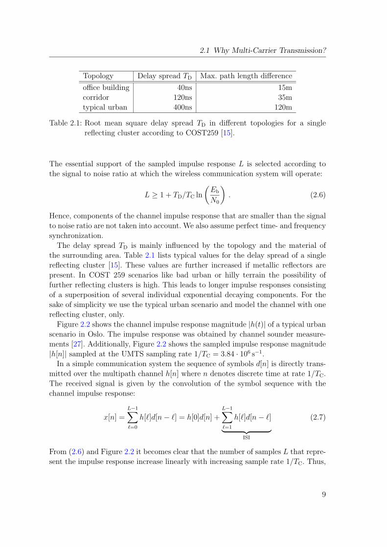
Figure 2.2 shows the channel impulse response magnitude |h(t)| of a typical urban
scenario in Oslo. The impulse response was obtained by channel sounder measure-
ments [27]. Additionally, Figure 2.2 shows the sampled impulse response magnitude
|h[n]| sampled at the UMTS sampling rate 1/TC = 3.84 · 106 s−1.
In a simple communication system the sequence of symbols d[n] is directly trans-
mitted over the multipath channel h[n] where n denotes discrete time at rate 1/TC.
The received signal is given by the convolution of the symbol sequence with the
channel impulse response:
x[n] =L−1∑
`=0
h[`]d[n − `] = h[0]d[n] +L−1∑
`=1
h[`]d[n − `]
︸ ︷︷ ︸
ISI
(2.7)
From (2.6) and Figure 2.2 it becomes clear that the number of samples L that repre-
sent the impulse response increase linearly with increasing sample rate 1/TC. Thus,
9
2 Multi-Carrier Code Division Multiple Access (MC-CDMA)
−1 −0.5 0 0.5 1 1.5 2 2.5 3 3.50
5
10
15
20
25
30
t [µs]
20lo
g|h
(t)|
[dB
]
Figure 2.2: Impulse response magnitude |h(t)| obtained through channel sounder
measurement in an urban scenario in Oslo [27]. Additionally, we also
depict the sampled impulse response magnitude |h[`]| sampled at the
UMTS sampling rate 1/TC = 3.84 · 106 s−1. The time origin was placed
at τ0, the time delay of the first arriving wavefront.
the inter-symbol interference (ISI) described by the second term in (2.7) increases
too. The application of a time-domain equalizer is the classical approach to remove
the inter-symbol interference. However, a time-domain equalizer gets prohibitively
complex with increasing data rate since the number of operations necessary grows
with O(L2).
In the next section we will introduce orthogonal frequency division multiplex-
ing (OFDM). This is a technique that is able to avoids inter-symbol interference
completely [11].
2.2 Orthogonal Frequency Division Multiplexing
(OFDM)
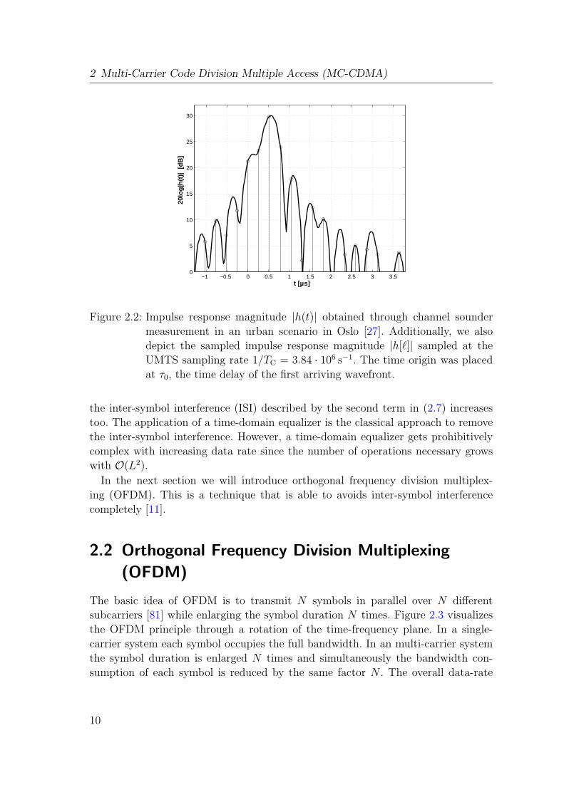
The basic idea of OFDM is to transmit N symbols in parallel over N different
subcarriers [81] while enlarging the symbol duration N times. Figure 2.3 visualizes
the OFDM principle through a rotation of the time-frequency plane. In a single-
carrier system each symbol occupies the full bandwidth. In an multi-carrier system
the symbol duration is enlarged N times and simultaneously the bandwidth con-
sumption of each symbol is reduced by the same factor N . The overall data-rate
10
2.2 Orthogonal Frequency Division Multiplexing (OFDM)
t
f
t
f
0 0 N
d[0
]
d[0]
d[1]
d[2]
d[3]
d[4]
d[5]
d[6]
d[7]
d[1
]
d[2
]
d[3
]
d[4
]
d[5
]
d[6
]
d[7
]
single carrier multi carrier
TC
TC
Figure 2.3: We illustrate the difference between a single-carrier and a multi-carrier
system through a rotation of the time-frequency plane. The transmitted
data symbols are denoted d[1] . . . d[8]. The multi-carrier system uses N =
8 subcarriers.
f
fq
fq+1
0
Df
1
magnitude
. . . . . .
Figure 2.4: Subcarrier frequency-spectra in an OFDM system. The subcarrier have
bandwidth ∆f . The center frequency of subcarrier q is denoted by fq.
and bandwidth consumption is kept constant trough parallel transmission over N
independent subcarriers.
The subcarrier spectra overlap, as depicted in Figure 2.4. However, if the center
frequency of each subcarrier q is chosen as
fq = q/(NTC) (2.8)
for q ∈ {0, . . . , N − 1} the subcarriers are orthogonal despite their overlapping
spectra. OFDM is a special case of a multi-carrier scheme with overlapping but
orthogonal subcarriers.
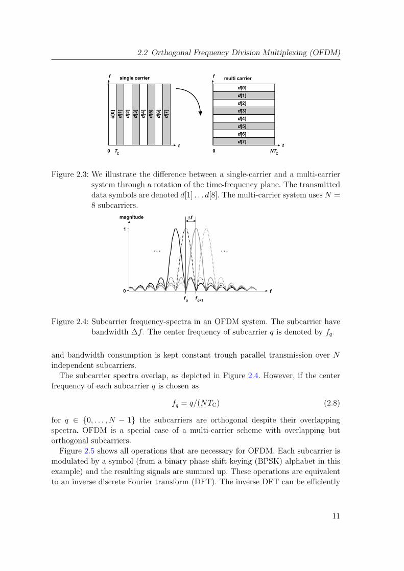
Figure 2.5 shows all operations that are necessary for OFDM. Each subcarrier is
modulated by a symbol (from a binary phase shift keying (BPSK) alphabet in this
example) and the resulting signals are summed up. These operations are equivalent
to an inverse discrete Fourier transform (DFT). The inverse DFT can be efficiently
11
2 Multi-Carrier Code Division Multiple Access (MC-CDMA)
t t
t t t
t t
f
2*f
3*f
1
1
1
subcarriers modulatedsubcarriers
symbols(BPSK)
*(+1)
*(+1)
*(-1) +
Figure 2.5: OFDM needs the following processing steps: First the subcarriers are
multiplied by the individual data symbols, then the resulting signals are
added together.
t
TS
Figure 2.6: Cyclic prefix insertion: A copy of the signal tail is inserted at the begin-
ning of each OFDM symbol.
implemented by means of the inverse fast Fourier transform. The existence of such
an efficient algorithm for the actual implementation is one major reason for the
widespread application of OFDM.
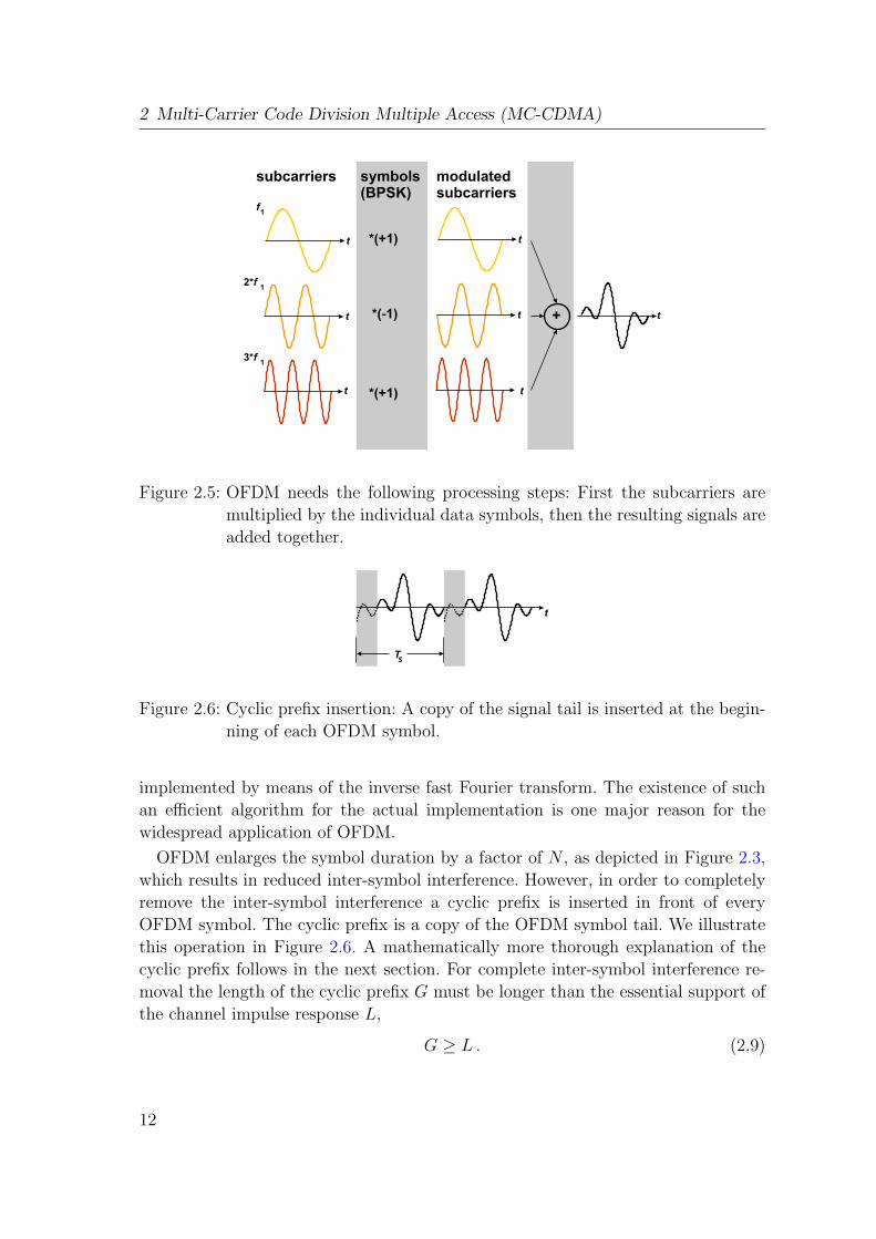
OFDM enlarges the symbol duration by a factor of N , as depicted in Figure 2.3,
which results in reduced inter-symbol interference. However, in order to completely
remove the inter-symbol interference a cyclic prefix is inserted in front of every
OFDM symbol. The cyclic prefix is a copy of the OFDM symbol tail. We illustrate
this operation in Figure 2.6. A mathematically more thorough explanation of the
cyclic prefix follows in the next section. For complete inter-symbol interference re-
moval the length of the cyclic prefix G must be longer than the essential support of
the channel impulse response L,
G ≥ L . (2.9)
12
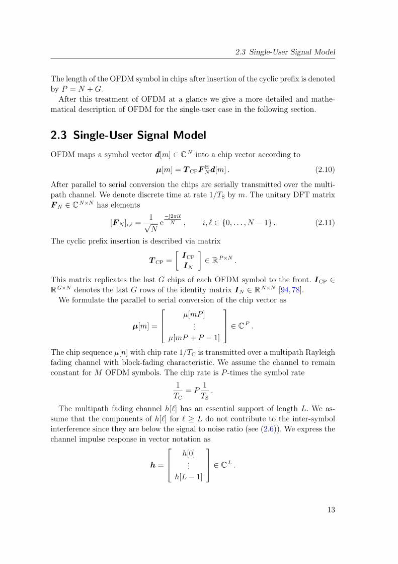
2.3 Single-User Signal Model
The length of the OFDM symbol in chips after insertion of the cyclic prefix is denoted
by P = N + G.
After this treatment of OFDM at a glance we give a more detailed and mathe-
matical description of OFDM for the single-user case in the following section.
2.3 Single-User Signal Model
OFDM maps a symbol vector d[m] ∈ CN into a chip vector according to
µ[m] = T CPF HNd[m] . (2.10)
After parallel to serial conversion the chips are serially transmitted over the multi-
path channel. We denote discrete time at rate 1/TS by m. The unitary DFT matrix
F N ∈ CN×N has elements
[F N ]i,` =1√N
e−j2πi`
N , i, ` ∈ {0, . . . , N − 1} . (2.11)
The cyclic prefix insertion is described via matrix
T CP =
[ICP
IN
]
∈ RP×N .
This matrix replicates the last G chips of each OFDM symbol to the front. ICP ∈R
G×N denotes the last G rows of the identity matrix IN ∈ RN×N [94, 78].
We formulate the parallel to serial conversion of the chip vector as
µ[m] =
µ[mP ]...
µ[mP + P − 1]
∈ C
P .
The chip sequence µ[n] with chip rate 1/TC is transmitted over a multipath Rayleigh
fading channel with block-fading characteristic. We assume the channel to remain
constant for M OFDM symbols. The chip rate is P -times the symbol rate
1
TC
= P1
TS
.
The multipath fading channel h[`] has an essential support of length L. We as-
sume that the components of h[`] for ` ≥ L do not contribute to the inter-symbol
interference since they are below the signal to noise ratio (see (2.6)). We express the
channel impulse response in vector notation as
h =
h[0]...
h[L − 1]
∈ C
L .
13
2 Multi-Carrier Code Division Multiple Access (MC-CDMA)
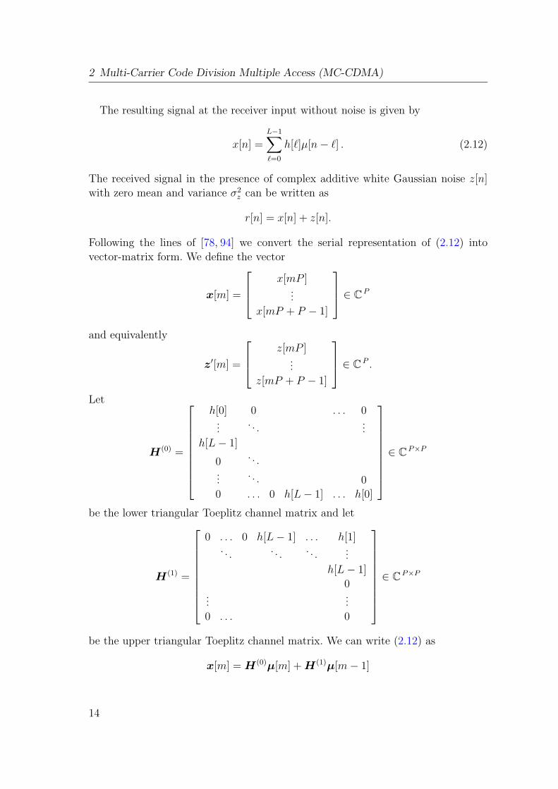
The resulting signal at the receiver input without noise is given by
x[n] =L−1∑
`=0
h[`]µ[n − `] . (2.12)
The received signal in the presence of complex additive white Gaussian noise z[n]
with zero mean and variance σ2z can be written as
r[n] = x[n] + z[n].
Following the lines of [78, 94] we convert the serial representation of (2.12) into
vector-matrix form. We define the vector
x[m] =
x[mP ]...
x[mP + P − 1]
∈ C
P
and equivalently
z′[m] =
z[mP ]...
z[mP + P − 1]
∈ C
P .
Let
H(0) =
h[0] 0 . . . 0...
. . ....
h[L − 1]
0. . .
.... . . 0
0 . . . 0 h[L − 1] . . . h[0]
∈ CP×P
be the lower triangular Toeplitz channel matrix and let
H(1) =
0 . . . 0 h[L − 1] . . . h[1]. . . . . . . . .
...
h[L − 1]
0...
...
0 . . . 0
∈ CP×P
be the upper triangular Toeplitz channel matrix. We can write (2.12) as
x[m] = H(0)µ[m] + H (1)µ[m − 1]
14

2.3 Single-User Signal Model
where the second term represents the inter-symbol interference between two consec-
utive OFDM symbols.
At the receiver the cyclic prefix of length G is removed, and a DFT is performed on
the remaining N chips. The cyclic prefix removal can be represented by the matrix
RCP = [0N×GIN ] ∈ RN×P
which removes the first G entries from the vector x[m] ∈ CP if the product RCPx[m]
is formed. As long as (2.9) holds,
RCPH(1) = 0N×P ,
which indicates that the inter-symbol interference between two consecutive OFDM
symbols is completely eliminated.
Finally, the received signal can be written as:
y[m] = FRCP(x[m] + z′[m]) = FRCPH(0)µ[m] + FRCPz′[m]
= FRCPH(0)T CPF Hd[m] + FRCPz′[m]
= FHF Hd[m] + FRCPz′[m] (2.13)
where H ∈ CN×N is the overall circulant channel matrix. This matrix can be
decomposed as
H = RCPH(0)T CP = F Hdiag(g)F (2.14)
where the frequency response g ∈ CN is defined as the DFT of the channel impulse
response
g =√
NF N×Lh .
Equation (2.14) describes the essential mathematical footing of OFDM. The
Toeplitz structure channel matrix H(0) is circularized by insertion of the cyclic
prefix. Therefore, the columns of the DFT matrix are exact eigenvectors and the
resulting channel matrix diag (g) has diagonal structure. The inversion of diag (g),
which is necessary for channel equalization, has complexity O(N). In contrast, the
channel matrix in a single-carrier system has full Toeplitz structure. The inversion
of a Toeplitz matrix is an operation with complexity O(N2).
Using (2.14) we write (2.13) as
y[m] = diag(g)d[m] + z[m], (2.15)
where the elements of z[m] = FRCPz′[m], denoted by z[m, q], are white with vari-
ance σ2z . Hence, the covariance matrix of z[m] has diagonal structure with identical
elements
Rz[m] = E{FRCPz[m]z[m]HRHCPF H}
= σ2zFRCPIP RH
CPF H
= σ2zIN .
15
2 Multi-Carrier Code Division Multiple Access (MC-CDMA)
0 dB
-4
-8
3 MHz210f
magnitude
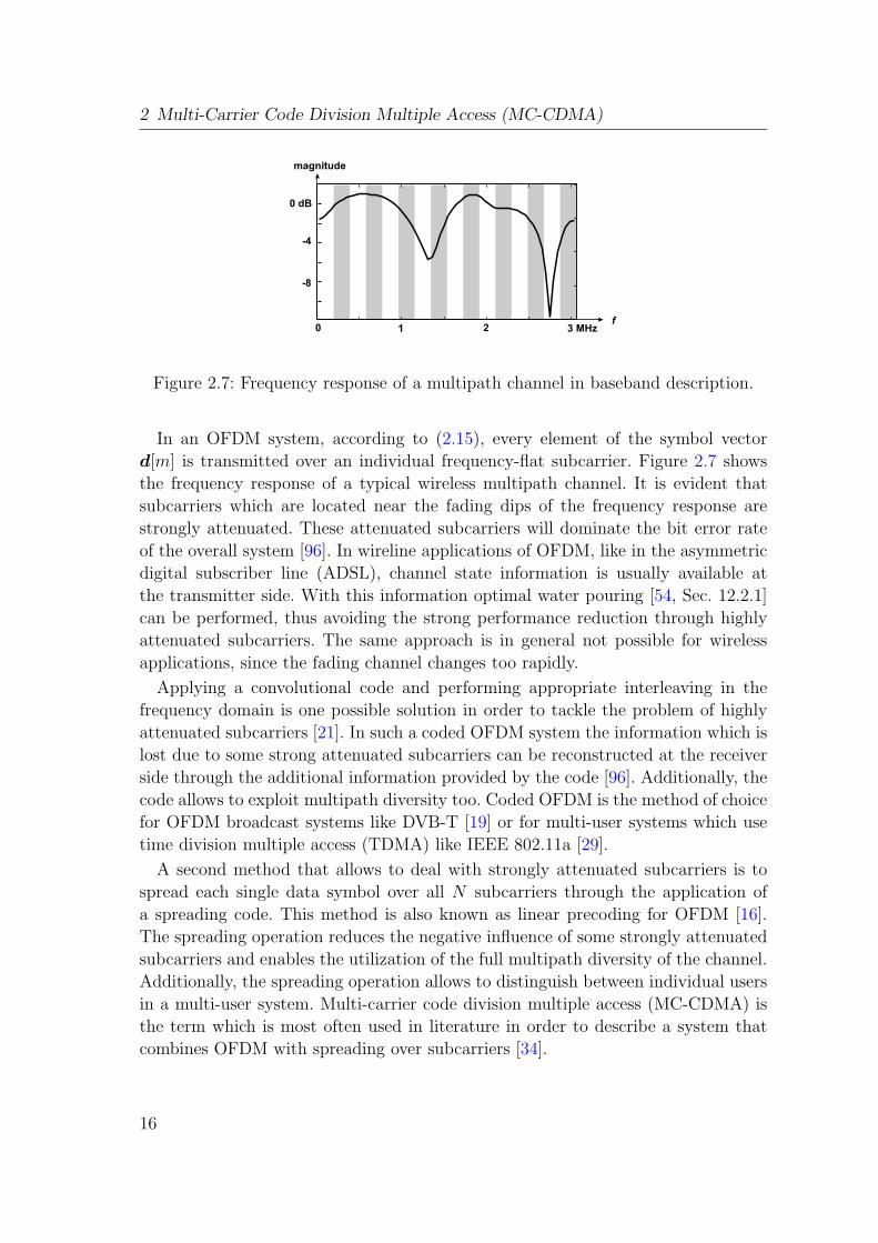
Figure 2.7: Frequency response of a multipath channel in baseband description.
In an OFDM system, according to (2.15), every element of the symbol vector
d[m] is transmitted over an individual frequency-flat subcarrier. Figure 2.7 shows
the frequency response of a typical wireless multipath channel. It is evident that
subcarriers which are located near the fading dips of the frequency response are
strongly attenuated. These attenuated subcarriers will dominate the bit error rate
of the overall system [96]. In wireline applications of OFDM, like in the asymmetric
digital subscriber line (ADSL), channel state information is usually available at
the transmitter side. With this information optimal water pouring [54, Sec. 12.2.1]
can be performed, thus avoiding the strong performance reduction through highly
attenuated subcarriers. The same approach is in general not possible for wireless
applications, since the fading channel changes too rapidly.
Applying a convolutional code and performing appropriate interleaving in the
frequency domain is one possible solution in order to tackle the problem of highly
attenuated subcarriers [21]. In such a coded OFDM system the information which is
lost due to some strong attenuated subcarriers can be reconstructed at the receiver
side through the additional information provided by the code [96]. Additionally, the
code allows to exploit multipath diversity too. Coded OFDM is the method of choice
for OFDM broadcast systems like DVB-T [19] or for multi-user systems which use
time division multiple access (TDMA) like IEEE 802.11a [29].
A second method that allows to deal with strongly attenuated subcarriers is to
spread each single data symbol over all N subcarriers through the application of
a spreading code. This method is also known as linear precoding for OFDM [16].
The spreading operation reduces the negative influence of some strongly attenuated
subcarriers and enables the utilization of the full multipath diversity of the channel.
Additionally, the spreading operation allows to distinguish between individual users
in a multi-user system. Multi-carrier code division multiple access (MC-CDMA) is
the term which is most often used in literature in order to describe a system that
combines OFDM with spreading over subcarriers [34].
16

2.4 Multi-User Signal Model
data encoder interl. mapper
N N
IFFT,
cyclic prefixP
pk[m]
sk P/S
µk[n]
hk[n]
µµµk[m] xk[n]
N
bk[m]
r[n]
z[n]
χk[m′′] ck[m′]
other users
αk
Figure 2.8: Model for the MC-CDMA transmitter and block-fading channel in the
uplink.
Because of all these mentioned benefits we will use MC-CDMA as the basic trans-
mission concept throughout this thesis. In the next section we introduce MC-CDMA
in more detail for the multi-user case in the uplink.
2.4 Multi-User Signal Model
Figure 2.8 shows the block structure of an MC-CDMA transmitter for the uplink.
The transmission is block oriented, a data block consists of M − J OFDM data
symbols and J OFDM pilot symbols. Each user transmits quadrature phase shift
keying (QPSK) modulated symbols bk[m] with symbol rate 1/TS. There are K users
in the system, the user index is denoted by k. Each symbol is spread by a user
specific spreading sequence sk ∈ CN . The spreading sequence sk has independent
identically distributed (i.i.d.) elements s[n] chosen with equal probability from the
QPSK constellation set1 {±1 ± j}/√
2N . Therefore, the spreading sequence fulfills
‖sk‖2 = 1 for k ∈ {1, . . . , K} .
In Section 2.5.1 we will treat the spreading sequence selection in more detail.
The data symbols bk[m] result from the convolutionally encoded, randomly inter-
leaved and QPSK modulated (with symbol mapper rate RS = 2) binary information
sequence χk[m′′] of length RSRC(M − J) by applying Gray labelling. The code rate
is denoted by RC. The amplitude of user k is denoted by αk. We do not take into
account path loss and assume perfect power control, thus
αk = 1 for k ∈ {1, . . . , K} .
1The expression {±1 ± j} is a shorthand notation for the set {+1 + j,+1 − j,−1 − j,−1 + j}.
17

2 Multi-Carrier Code Division Multiple Access (MC-CDMA)
To allow for pilot symbol insertion at the beginning of each data block the M − J
data symbols for a block of length M satisfy
bk[m] ∈ {±1 ± j} 1√2
for m ∈ {J, . . . ,M − 1} ,
and
bk[m] = 0 for m ∈ {0, . . . , J − 1} .
After the spreading operation a pilot symbol vector pk[m] ∈ CN with elements
pk[m, q] is added
dk[m] = skbk[m] + pk[m] . (2.16)
The elements of the pilot vector pk[m, q] are i.i.d. chosen with equal probability from
the QPSK symbol set {±1 ± j}/√
2N for m ∈ {0, . . . , J − 1}, otherwise
pk[m] = 0N for m ∈ {J, . . . ,M − 1} .
Finally, an N point inverse DFT is performed and a cyclic prefix of length G is
inserted. We insert (2.16) into (2.10) and obtain the transmitted chip sequence for
user k
µk[m] = T CPF HN (skbk[m] + pk[m]) .
The received signal for user k after the DFT operation and the cyclic prefix removal
can be expressed as
yk[m] = diag (gk) (skbk[m] + pk[m]) + z[m] , (2.17)
where
gk =√
NF N×Lhk
with elements gk[q] for q ∈ {0, . . . , N−1}. We define the effective spreading sequence
sk = diag(gk)sk (2.18)
and represent the multi-user system by
y[m] = Sb[m] +K∑
k=1
diag(gk)pk[m] + z[m] (2.19)
where the effective spreading matrix is defined as
S = [s1, . . . , sK ] ∈ CN×K
and
b[m] =
b1[m]...
bK [m]
∈ C
K (2.20)
contains the information symbols for K users at time index m.
18

2.5 Multi-User Detection
2.5 Multi-User Detection
At the base station the multi-user detector has the task to find the most likely
transmitted sequence of data vectors b[m] given the received vectors y[m]. This is
a special class of a vector-classification problem that is generally np-complete. A
bank of K linear filters matched to the K effective spreading sequences form a set
of sufficient statistics for the estimation of all users data [75]:
ξ[m] = SHy[m]. (2.21)
This means that by using ξ[m] no information is lost. If we define the correlation
matrix
RS = SHS (2.22)
the MC-CDMA system can be described by
ξ[m] = RSb[m] + SHz[m]. (2.23)
2.5.1 Spreading Sequences
As already mentioned, the aim of the spreading operation is twofold: First, it dis-
tributes the information of the transmitted data symbol over all subcarrier and
second, it is used in order to differentiate the individual users. For orthogonal Walsh-
Hadamard spreading sequences and frequency-flat channels the correlation matrix
RS will be the identity matrix and user separation will be optimal. For frequency-
selective channels this is not true anymore because of (2.18). For sequences with
length N there exist N different orthogonal sequences. The maximum number of
users is therefore limited to N . We define the load as
β =K
N.
For random spreading sequences with length N there exist 2N different sequences
(for a BPSK alphabet). Thus, by using random spreading sequences the load can be
increased above 1. The lost orthogonality of the spreading sequences is of no great
impact, since the effective spreading sequences are not orthogonal anyway.
2.5.2 Linear Detector Types
The optimum maximum likelihood detector operating on ξ[m] is prohibitively com-
plex. Hence, we resort to suboptimum linear multi-user detectors [50]. After linear
19

2 Multi-Carrier Code Division Multiple Access (MC-CDMA)
filtering, denoted by matrix L, a hard decision is performed to obtain an estimate
for the transmitted symbols
b[m] = quantX
(Lξ[m]),
with
quantX
(w) = argminw∈X
|w − w|
where X denotes the symbol set. For the QPSK constellation we define
X = {±1 ± j}/√
2.
The matched-filter receiver is optimal with respect to the signal to noise ratio
for orthogonal spreading sequences sk in frequency-flat channels. The output of the
filter bank ξ[m] (the sufficient statistics) is directly used in order to detect the data
symbols, i.e.
L = I.
In a frequency-selective channel the orthogonality of the spreading sequences is
destroyed by the effect of the channel, mathematically described by (2.18). Therefore,
a simple matched-filter receiver has poor performance that degrades rapidly when
the number of users is increased because of the multi-access interference.
Better performance can be achieved with the decorrelating receiver. The decorre-
lator (also known as zero forcing solution) follows from the approximation X ≈ C
and is given by
L = R−1
S.
The decorrelator completely suppresses all interference but enhances the noise [75,
Sec. 5]. This effect can be seen in Figure 2.9. In the low signal to noise region the
decorrelating detector performs even worse than the matched filter.
A common approach in estimation theory is to choose a function L(ξ) that mini-
mizes the mean square error. Because vector b[m] is not Gaussian the exact solution
is challenging. It is common to minimize the mean square error
E{(b[m] − Lξ[m])H(b[m] − Lξ[m])} (2.24)
within the restricted set of linear functions that can be represented by matrix L.
The solution of the minimization problem results in the linear MMSE filter given by
L =(RS + σ2
zI)−1
.
The complexity of the linear MMSE filter is identical to the one of the decorrelator
but the performance for low signal to noise ratios is enhanced.
20

2.6 Iterative Multi-User Detection
0 2 4 6 8 10 12 14 16 1810
−4
10−3
10−2
10−1
Eb/N
0 [dB]
BE
R
MF, 32 userDEC, 32 userMMSE, 32 userSUB
Figure 2.9: Bit error rate (BER) versus Eb/N0 for an MC-CDMA uplink with K =
32 users and spreading length N = 64 for different linear multi-user
detectors: matched-filter (MF), decorrelator (DEC), and linear MMSE
filter. The single-user bound (SUB) is shown for the linear MMSE filter.
We demonstrate this with the comparison in Figure 2.9 where the performance of
the matched-filter, the decorrelator, and the linear MMSE filter is shown in terms
of bit error rate versus Eb/N0. The energy per bit is denoted by Eb and N0 denotes
the noise power spectral density. We simulate an MC-CDMA uplink with K = 32
user and spreading length N = 64. The Rayleigh fading channel is perfectly known
to the receiver. The single-user bound is defined as the performance for one user
with perfect channel knowledge. The single-user bound was simulated using the
linear MMSE detector. The comparison makes clear, that the linear MMSE detector
performs best and the performance difference to the decorrelator is largest in the low
signal to noise region. Based on this performance results and its moderate complexity
we will use the linear MMSE detector throughout this thesis.
2.6 Iterative Multi-User Detection
In iterative receivers, the information gained about the transmitted symbols is used
in subsequent iterations in order to reduce the interference from other users [14]. Soft
symbols bk[m] instead of hard decisions bk[m] are used to avoid error propagation. A
convolutional code is used and the BCJR algorithm [6] is applied in order to obtain
soft output values on the received code symbols. The iterative MC-CDMA receiver
21

2 Multi-Carrier Code Division Multiple Access (MC-CDMA)
... ...
... .........
......
...... ... ...
deinterl.
deinterl.
interl.
interl.
channeldecoder
channeldecoder
mapper
demapper
demapper
PIC,
MMSE
estimator
drop prefix,
FFTS/P
r(n)
P N
r[m] y[m]
.
.
.
g1...K
χK [m′′]
APP(ck[m′])
EXT(ck[m′])
w1[m]
wK [m] w′
K[m′]
w′
1[m′]
χ1[m′′]
b′k[m]
bk[m]
mapperchannel
Figure 2.10: Schematic model of an MC-CDMA receiver that performs iterative joint
channel-estimation and multi-user detection.
detects the data b[m] using the received vector y[m], the effective spreading matrix
S(i)
, and the feedback extrinsic probability (EXT) on the code bits at iteration step
i denoted by Pr(EXT){c(i)k [m′] = +1}. Figure 2.10 shows the structure of this iterative
receiver.
The frequency-selective nature of the channel implies to build a filter which is
matched to the effective spreading sequence s(i)k . For the moment, it is only of in-
terest that the channel estimator supplies an estimate gk for the channel frequency
response of every user. The general optimization problem is therefore reduced to the
estimation of b[m]. In order to cancel the multi-access interference, we perform soft
parallel interference cancellation for user k:
y(i)k [m] = y[m] + s
(i)k b
(i)k [m] − S
(i)b
(i)[m]. (2.25)
Vector b(i)
[m] contains the soft symbol estimates that are computed from the extrin-
sic probability supplied by the decoding stage. When the extrinsic probabilities get
better from iteration to iteration and the channel is correctly estimated the parallel
interference cancelling removes the interference from all other users completely and
the detection problem is reduced to a single-user detection in Gaussian noise.
The soft symbol mapping for the QPSK alphabet is given by
bk[m] = Eb
(EXT){bk[m]} = Ec
(EXT){ck[2m]} + jEc
(EXT){ck[2m + 1]} (2.26)
where
Ec
(EXT){ck[m′]} = Pr(EXT){ck[m
′] = +1} − Pr(EXT){ck[m′] = −1}
= 2Pr(EXT){ck[m′] = +1} − 1 (2.27)
calculates the expectation over the alphabet of c which is {−1, +1} and
Pr(EXT){ck[m′] = +1} is the extrinsic probability supplied by the BCJR decoder.
22

2.7 Decoder
The notation E(EXT) is chosen to explicitly show that extrinsic probabilities are used
for the calculation of the expectation. In the next chapter about channel estimation
we will use soft symbols based on a-posteriori probabilities which will be indicated
through the notation E(APP).
The y(i)k [m] are further cleaned from noise and multi-access interference with a
successive linear MMSE filter
w(i)k [m] = (f
(i)k )Hy
(i)k [m] (2.28)
to obtain an estimate of the transmitted symbols bk[m]. An unbiased MMSE filter
for the MC-CDMA system can be found similarly to the MMSE detector given
in [14,51,80]. We omit the iteration index (·)(i) to allow for simpler notation,
fHk =
sHk (σ2
zI + SV SH)−1
sHk (σ2
zI + SV SH)−1sk
. (2.29)
Matrix V denotes the error covariance matrix of the soft symbols
V = E{(b[m] − b[m])(b[m] − b[m])H}
with diagonal elements
Vk,k = E{1 − |bk[m]|2} (2.30)
which are constant during iteration i, the other elements are assumed to be zero. In
this case we calculate the variance from all symbols in the block belonging to user
k and call the filter unconditional.
The expectation operator in (2.30) is implemented as empirical mean
Vk,k = E{1 − |bk[m]|2} =1
M
M−1∑
m=0
(1 − |bk[m]|2) , (2.31)
which is the case for all expectation operators in numerical simulations in this thesis,
if not noted otherwise.
2.7 Decoder
The iterative receiver feeds back soft values on code bits ck[m′] in order to get better
detection results and better channel estimates. The soft feedback values are either
computed from the so-called a-posteriori probability (APP) or the extrinsic proba-
bility (EXT) of the code bits through mapping to QPSK symbols. The soft-symbol
mapping from extrinsic probabilities is given in (2.26). A similar mapping from a-
posteriori probabilities (3.5) is used for the iterative channel estimation algorithm
that will be treated in the next chapter [35,80].
23

2 Multi-Carrier Code Division Multiple Access (MC-CDMA)
A soft-input soft-output decoder for binary convolutional codes, implemented us-
ing the BCJR algorithm [6], supplies these measures. The input values to the decoder
are the so called channel values w′k[m
′] derived from the linear MMSE-filter outputs
after demapping and deinterleaving. Additionally the decoder also needs an estimate
of the noise variance
σ2z,k =
1
2M
2M−1∑
m′=0
|w′k[m
′] − µw′,k|2 ,
where the mean value of the absolute channel values is estimated through
µw′,k =1
2M
2M−1∑
m′=0
|w′k[m
′]| .
The explicit estimation of µw′,k is necessary because during the first iterations the
channel estimates are not accurate and thus the linear MMSE filter (2.29) is not
truly unbiased.
The a-posteriori probability for the code symbol being +1 if the channel value
w′k[m
′] is observed is given by
Pr(APP) {ck[m′] = +1} = Pr {ck[m
′] = +1 | w′k[m
′]} . (2.32)
The link between a-posterior probability and extrinsic probability is established via
Pr(APP) {ck[m′] = +1} ∝ Pr(EXT) {ck[m
′] = +1}Pr {w′k[m
′] | ck[m′] = +1} , (2.33)
where the last expression denotes the channel transition function, which is as con-
ditional Gaussian probability density function
Pr {w′k[m
′] | ck[m′] = +1} =
1√
2πσ2z,k
exp
(
−|w′k[m
′] − µw′,k|22σ2
z,k
)
. (2.34)
Estimating σ2z,k after the linear MMSE filter we model the residual multiple access
interference as additive Gaussian noise (2.34).
24
3 Iterative Channel Estimation for
Block-Fading Channels
Accurate channel estimation is crucial for the performance of any type of multi-user
receiver. This is made obvious by (2.18); a filter matched to the effective spreading
sequence depends directly on the quality of the channel estimate.
Various blind channel estimation schemes have been proposed in the literature
for MC-CDMA. All these schemes suffer from an inherent phase ambiguity [73]. For
coherent detection, which is necessary for multi-user detection schemes, it would be
necessary to introduce some sort of pilot symbols to resolve this ambiguity. Further-
more, the popular blind subspace method limits the maximum number of users in
the system to K ≤ N −L, see [33,44,45,82]. We propose a new iterative pilot based
channel estimation scheme that can be applied to overloaded systems K > N and
allows for coherent detection.
3.1 Iterative Least-Square Channel Estimation
We use a random time domain pilot sequence pk[m, q] with i.i.d. elements that is
J symbols long and unique for every user k and subcarrier q. This approach was
inspired by equivalent approaches for direct sequence (DS)-CDMA in [13, 80] and
the analysis in [94].
Figure 3.1 gives a schematic representation of the channel estimation scheme.
Please note that the pilot sequence is a sequence in time while the spreading se-
quence, which is used to spread the information of a data symbol bk[m] over all
subcarriers, is applied in the frequency domain. Therefore, this scheme allows to
decouple the user specific identification sequences that are used for data detection
and for channel estimation.
The MC-CDMA transmission described by the signal model (2.17) takes place
over N independent parallel frequency-flat channels respectively subcarriers. We
25

3 Iterative Channel Estimation for Block-Fading Channels
s n[ ]k
pk
spreading sequence
pilotsequence subcarrier =q 1
2
3
4
J=4 pilots M-J data symb.
21 5 63 74 8 ...
[ ,1]m
Figure 3.1: Channel estimation scheme for an iterative MC-CDMA receiver. The
pilot sequence in time for user k on subcarrier q is denoted by pk[m, q]
where m denotes discrete time. The spreading sequence sk[n] is applied
in the frequency domain.
rewrite (2.17) as a set of equations for every subcarrier q ∈ {0, . . . , N − 1},
y[m, q] =K∑
k=1
gk[q]dk[m, q] + z[m, q] ,
where
dk[m, q] = sk[q]bk[m] + pk[m, q] . (3.1)
Hence, a least-square estimate of the subcarrier coefficients gk[q] can be obtained
jointly for all K users but individually for every subcarrier q.
We define the vector
gq =
g1[q]...
gK [q]
∈ C
K
containing the channel coefficients of all K users for subcarrier q. Furthermore, we
introduce the notation
yq =
y[0, q]...
y[M − 1, q]
∈ C
M
denoting the received symbol sequence on subcarrier q for a single data block. With
these definitions we can write
yq = Dqgq + zq , (3.2)
where the matrix Dq ∈ CM×K is defined as
Dq =
d1[0, q] . . . dK [0, q]...
. . ....
d1[M − 1, q] . . . dK [M − 1, q]
, (3.3)
26

3.1 Iterative Least-Square Channel Estimation
containing the transmitted symbols for all K users on subcarrier q.
For the channel estimation task the J pilot symbols pk[m, q] for m ∈ {0, . . . , J−1}in (3.1) are known. The remaining M−J data symbols bk[m] for m ∈ {J, . . . ,M−1}are not known. We replace them by soft symbols b′k[m] that are calculated from the a-
posteriori probabilities obtained in the previous iteration. This enables us to obtain
refined channel estimates if the soft symbols gets more certain from iteration to
iteration. For the first iteration the soft symbols b′k[m] are set to zero.
We define the soft symbol matrix Dq ∈ CM×K equivalent to (3.3) by replacing
dk[m, q] with
dk[m, q] = sk[q]b′k[m] + pk[m, q] . (3.4)
The soft symbols b′k[m] are defined according to
b′k[m] = Eb
(APP){bk[m]} = Ec
(APP){ck[2m]} + jEc
(APP){ck[2m + 1]} (3.5)
where
Ec
(APP){ck[m′]} = Pr(APP){ck[m
′] = +1} − Pr(APP){ck[m′] = −1}
= 2Pr(APP){ck[m′] = +1} − 1 ,
and Pr(APP){ck[m′] = +1} is the a-posteriori probability supplied by the BCJR
decoder. The code bits c[m′] are from the set {+1,−1}.Finally, the least-square channel estimator is given by
g′q =
(
DH
q Dq
)−1
DH
q yq. (3.6)
After estimating the subcarrier coefficients for all subcarriers we can further reduce
the noise by exploiting their correlation since the channel impulse response in the
time domain hk possesses L < N taps:
gk = F N×LF HN×Lg′
k. (3.7)
The estimates gk are inserted in (2.18) to calculate the effective spreading sequences
which in turn are used by the parallel interference canceller (2.25) and the linear
MMSE detector (2.28).
The least square solution in (3.6) expects deterministic values in matrix D. How-
ever, this is not the case since we combine deterministic pilots with soft symbols.
The absolute values of the soft symbols in matrix Dq can be very small, particularly
during the first iteration and in overloaded systems, where
β = K/N > 1 , (3.8)
27

3 Iterative Channel Estimation for Block-Fading Channels
0 2 4 6 8 10 12 14−20
−15
−10
−5
0
n
10lo
g(η[
n]2 )
[dB
]
TD=1µs
TD=0.26µs
Figure 3.2: Power delay profile η2[`] with (root mean square) delay spread TD ∈{0.26, 1}µs sampled at rate 1/TC = 3.84 · 106 s−1. The normalized delay
spread LD = TD/TC ∈ {1, 4}. We plot L = 15 significant channel taps.
due to strong interference. This leads to strongly biased channel estimates and slow
convergence of the iterative receiver. We apply a partial heuristic solution through
scaling by√
N/L in the first iteration, i.e.
g(1)k = F N×LF H
N×Lg′k(1)
√
N
L.
Furthermore, we normalize each column of Dq to√
M/N , so that the Frobenius
norm ‖Dq‖F stays constant. In Section 3.2 we will present a more systematic solution
based on the MMSE theory.
3.1.1 Simulation Parameters
The realizations of the Rayleigh fading channel are calculated using the exponential
power delay profile (2.4) with a delay spread TD ∈ {0.26, 1}µs. We use a chip rate of
1/TC = 3.84·106 s−1 as in UMTS. The normalized delay spread LD = TD/TC ∈ {1, 4}.We obtain an essential support of the channel impulse response (2.6) of L = 15 for
a maximum Eb/N0 = 15 dB.
The OFDM transmission uses N = 64 subcarriers and each OFDM symbol includ-
ing the cyclic prefix has length of P = G + N = 79 chips. The spreading sequence
has length N = 64 equal to the number of subcarriers. The convolutional code used
is a non-systematic, non-recursive, four state, rate RC = 1/2 code with generator
28
3.1 Iterative Least-Square Channel Estimation
0 2 4 6 8 10 12 1410
−4
10−3
10−2
10−1
Eb/N
0 [dB]
BE
R
01. iteration, LD=1
02. iteration, LD=1
03. iteration, LD=1
04. iteration, LD=1
05. iteration, LD=1
06. iteration, LD=1
07. iteration, LD=1
SUB, LD=1
07. iteration, LD=4
SUB, LD=4
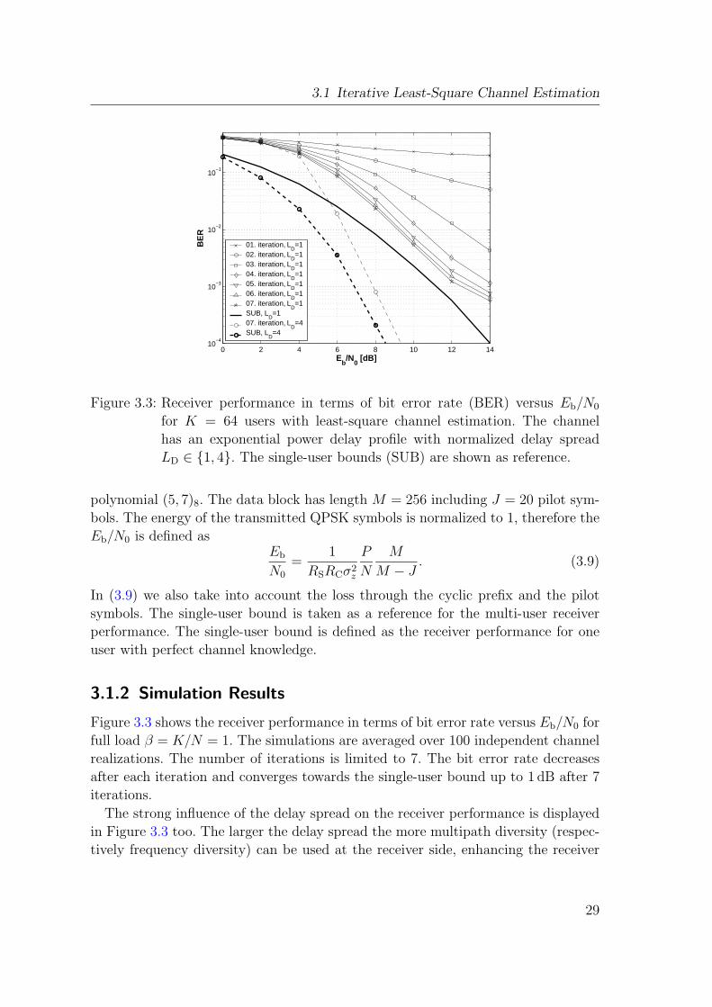
Figure 3.3: Receiver performance in terms of bit error rate (BER) versus Eb/N0
for K = 64 users with least-square channel estimation. The channel
has an exponential power delay profile with normalized delay spread
LD ∈ {1, 4}. The single-user bounds (SUB) are shown as reference.
polynomial (5, 7)8. The data block has length M = 256 including J = 20 pilot sym-
bols. The energy of the transmitted QPSK symbols is normalized to 1, therefore the
Eb/N0 is defined asEb
N0
=1
RSRCσ2z
P
N
M
M − J. (3.9)
In (3.9) we also take into account the loss through the cyclic prefix and the pilot
symbols. The single-user bound is taken as a reference for the multi-user receiver
performance. The single-user bound is defined as the receiver performance for one
user with perfect channel knowledge.
3.1.2 Simulation Results
Figure 3.3 shows the receiver performance in terms of bit error rate versus Eb/N0 for
full load β = K/N = 1. The simulations are averaged over 100 independent channel
realizations. The number of iterations is limited to 7. The bit error rate decreases
after each iteration and converges towards the single-user bound up to 1 dB after 7
iterations.
The strong influence of the delay spread on the receiver performance is displayed
in Figure 3.3 too. The larger the delay spread the more multipath diversity (respec-
tively frequency diversity) can be used at the receiver side, enhancing the receiver
29

3 Iterative Channel Estimation for Block-Fading Channels
0 2 4 6 8 10 12 1410
−4
10−3
10−2
10−1
Eb/N
0 [dB]
BE
R
01. iteration, LD=1
02. iteration, LD=1
03. iteration, LD=1
04. iteration, LD=1
05. iteration, LD=1
06. iteration, LD=1
07. iteration, LD=1
SUB, LD=1
07. iteration, LD=4
SUB, LD=4
Figure 3.4: Receiver performance in terms of bit error rate (BER) versus Eb/N0 for
K = 80 users with least-square channel estimation. The channel has an
exponential decaying power delay profile with normalized delay spread
LD ∈ {1, 4}.
performance.
Figure 3.4 shows the same results for a moderately overloaded system with load
β = 1.25 for K = 80 users and normalized delay spread LD ∈ {1, 4}. The bit rate per
user is 44.8 kbit/s, the net bit rate per cell is 2.87 Mbit/s for 64 users and 3.58 Mbit/s
for 80 users.
The iterative receiver uses pilot symbols only for channel estimation in the first
iteration. These channel estimates are used in the multi-user detector in order to
calculate the effective spreading sequence and perform data detection. This is why
the bit error rate curve of the first iteration is identical with the performance of a
non-iterative linear MMSE multi-user detectors with imperfect channel knowledge.
In the second iteration soft symbols are supplied by the BCJR decoder which are
used in the parallel interference canceller in order to reduce the interference by other
users. Additionally, the soft symbols also help to enhance the channel estimation
quality. This leads to continuous performance improvements between iteration 1
and iteration 7 as can be clearly seen in Figure 3.3 and Figure 3.4. In a fully loaded
system and even in an overloaded system the reduction in bit error rate is in the
orders of 3 magnitudes after 7 iterations.
30
3.1 Iterative Least-Square Channel Estimation
3.1.3 Comparison Between MC-CDMA and DS-CDMA
It is well-known that the signal-models for MC-CDMA and DS-CDMA are similar
[50], and therefore many multi-user detection algorithms are applicable to both
MC-CDMA and DS-CDMA. However, the computational complexity of the channel
estimation algorithm for an MC-CDMA receiver is smaller than the one needed for
DS-CDMA.
In MC-CDMA the inter-symbol interference is removed through insertion of the
cyclic prefix, and channel equalization is performed in the frequency domain. The
complexity for the channel estimation is growing by O(NK3) in MC-CDMA where
N denotes the number of subcarriers and K the number of users. The term K3
is due to the necessary matrix inversion with dimension K × K which has to be
performed for N subcarriers individually.
In comparable DS-CDMA systems for UMTS time division duplex (TDD) the
complexity grows with O(L3K3) since the matrix to be inverted has dimension
LK × LK [80]. The time-domain channel estimation in DS-CDMA has to estimate
L channel taps for all K users jointly, thus raising its complexity. Whereas, in an
OFDM system the coefficients for every subcarrier can be estimated separately.
The essential support of the channel L determines the length of the cyclic prefix.
The number of subcarriers N is usually N > 5L, so that the spectral efficiency of the
system is still acceptable. The spectral efficiency of the system is determined by the
ratio L/(N +L). Thus, the channel estimation complexity advantage of MC-CDMA
is especially important at high data rates when L gets large.
3.1.4 Channel Estimation Error
Figure 3.4 presents the performance of an MC-CDMA system with load β = 1.25
in terms of bit error rate versus Eb/N0. The distance to the single-user bound is
increased compared to the results for load β = 1 that are shown in Figure 3.3. We
know from theoretical results that with perfect channel knowledge the performance
difference between K = 64 and K = 80 users should be much smaller [14]. Thus, we
analyze the channel estimation error in this section.
We define the mean square error of the channel estimates, so that we obtain a
measure of the channel estimation quality:
MSEBF =1
KL
K∑
k=1
∥∥∥hk − hk
∥∥∥
2
.
In Figure 3.5 we plot the mean square error of the channel estimate versus the
iteration number for a channel with exponential decaying power delay profile with
normalized delay spread LD = 1. It can be clearly seen, that the mean square error
31

3 Iterative Channel Estimation for Block-Fading Channels
1 2 3 4 5 6 710
−4
10−3
10−2
10−1
iterations
MS
E
Eb/N
0=0 dB
Eb/N
0=2 dB
Eb/N
0=4 dB
Eb/N
0=6 dB
Eb/N
0=8 dB
Eb/N
0=10 dB
Eb/N
0=12 dB
Eb/N
0=14 dB
Figure 3.5: Mean square error (MSE) of the channel estimates for K = 80 users with
least-square channel estimation for normalized delay spread LD = 1.
slightly increases after the 2nd iteration especially for a low signal to noise ratio.
This is due to the already mentioned fact, that the soft symbols in matrix Dq have
very small absolute values, particularly during the first iteration and in overloaded
systems (3.8) due to strong interference.
In the next section we develop an iterative channel estimation scheme based on
the MMSE theory in order to avoid this degradation of the channel estimation
performance with increasing number of users.
3.2 Iterative Linear Minimum Mean Square Error
Channel Estimation
Equation (3.5) makes clear, that the soft symbols are actually the expectation of the
data symbols given the received data vector and the current channel estimate after
the decoding process. Since the data symbols are from a constant modulus alphabet
we know their variance too,
var{bk[m]} = Eb
{(
bk[m] − Eb{bk[m]}
)2}
= 1 − b2k[m]. (3.10)
We take advantage of this information in the following, deriving a linear MMSE
multi-user channel estimator, enhancing the overall performance especially for over-
32

3.2 Iterative Linear Minimum Mean Square Error Channel Estimation
loaded systems. See also [74] for a related approach in a single-user scenario. Inde-
pendently in [3] a similar algorithm was derived using the concept of expectation
maximization (EM).
The individual subcarriers in an OFDM system are orthogonal. For this reason we
are able to estimate the subcarrier coefficient gk[q] individually for every subcarrier q
but jointly for all K users. We repeat the signal model (3.2) for the received symbol
block yq on subcarrier q which is given by
yq = Dqgq + zq .
In the previous section we obtained the channel coefficients using a least-square
estimator by approximating Dq with Dq. The matrix Dq contains deterministic
pilot symbols and statistical information in terms of expectation (3.5) about the
transmitted data symbols.
The minimization of the mean square estimation error is a widely used optimiza-
tion criterion in parameter estimation. We use this approach in order to estimate
the channel coefficients. In general, for a linear data model, if the observed data
and the unknown parameters are jointly Gaussian distributed, the resulting MMSE
estimator is a linear function of the data. In the model (3.2), we assume that the
channel coefficients in the vector gq are independent, complex Gaussian distributed
random variables, with zero mean and unit variance (which corresponds to Rayleigh
fading), while the symbols in the matrix Dq have a discrete distribution determined
by the QPSK symbol alphabet. The resulting distribution of the observed vector yq
is not Gaussian, thus the MMSE estimator is not linear. Due to the shape of the
probability density function f(yq), the derivation of the exact MMSE estimator is a
complicated task. Therefore, we constrain the channel estimator to be linear in yq.
We will omit the index q in the following derivations to simplify the notation.
The linear estimator can be expressed as
gLMMSE = Ay,
where the matrix A satisfies the Wiener-Hopf equation
CyyAH = Cyg .
The covariance matrices are given by (y, g and z are zero-mean and statistically
independent)
Cyy = Eb
Eg
Ez
{yyH
}= E
b
{DDH
}+ σ2
zIM (3.11)
Cyg = Eb
Eg
Ez
{ygH
}= E
b{D} , D, (3.12)
33

3 Iterative Channel Estimation for Block-Fading Channels
where the index under the expectation operator denotes the random variable with
respect to which the expectation is taken. Expectations with respect to b are com-
puted using APPs of data symbols, see (3.5). The linear MMSE estimator is then:
gLMMSE = CygHCyy
−1y
= DH(
Eb
{DDH
}+ σ2
zIM
)−1
y. (3.13)
If we want to calculate Eb{DDH} we have to take into account that due to the
independence of the users and the data symbols within one block, it holds:
Eb{b′k[m′]bk[m]} =
{b′k[m
′]bk[m], k′ 6= k,m′ 6= m
1, k′ = k,m′ = m(3.14)
for k, k′ ∈ {1, ..., K} and for m,m′ ∈ {0, 1, ...,M − 1}. Please refer to (3.5) for the
definition of the soft symbols bk[m].
With (3.14) we are able to write the expectation of the product Eb{DDH} as
product of expectations plus a correcting diagonal matrix Λ which takes (3.14) into
account
Eb{DDH} = E
b{D}E
b{DH} + Λ = DD
H+ Λ. (3.15)
The elements of the diagonal matrix Λ are defined as
[Λ]m,m =K∑
k=1
var{bk[m]} , (3.16)
where the soft-symbol variance from (3.10) is used.
Inserting (3.15) into (3.13) we obtain
gLMMSE = DH
DD
H+ Λ + σ2
zIM︸ ︷︷ ︸
,∆
−1
y. (3.17)
For the evaluation of this estimator it is necessary to invert an M -dimensional
matrix, which is computationally expensive. In order to reduce complexity we apply
the matrix inversion lemma to (3.17). The final expression yields
gLMMSE =(
DH∆
−1D + IK
)−1
DH∆
−1y. (3.18)
The rows of matrix D are scaled by the diagonal matrix ∆, taking into account the
variance of the noise and the variances of the soft-symbol estimates.
34

3.2 Iterative Linear Minimum Mean Square Error Channel Estimation
0 2 4 6 8 10 12 1410
−4
10−3
10−2
10−1
Eb/N
0 [dB]
BE
R
01. iteration02. iteration03. iteration04. iteration05. iteration06. iteration07. iterationSUB
Figure 3.6: Receiver performance in terms of bit error rate (BER) versus Eb/N0
for K = 80 users with linear MMSE channel estimation and normalized
delay spread LD = 1. For reference the single-user bound (SUB) is shown
too.
If the data symbols are known, then
bk[m] = bk[m],
thus Λ = 0, ∆ = σ2zIK and the estimator (3.18) becomes the exact MMSE estimator
(conditioned on the given D, g and y are jointly Gaussian, thus the linear MMSE
coincides with the exact MMSE estimator which becomes linear for jointly Gaussian
variables):
gMMSE|D =(DHD + σ2
zIK
)−1DHy. (3.19)
For the training part of the data block (the first J symbols), the estimator will
equal the exact MMSE estimator for the given pilot symbols. For the data part the
variances of the estimates of the unknown data symbols are taken into account by
the matrix ∆.
3.2.1 Simulation Results
The simulation results for this estimator are given in Figure 3.6 and Figure 3.7. The
parameters are the same as in the least-square case (see Section 3.1). If Figure 3.7
is compared with the results obtained with the least-square estimator in Figure 3.5,
it can be clearly seen that the mean square error is a monotonic decreasing function
of the iteration number and the Eb/N0, now. The bit error rate performance in
35

3 Iterative Channel Estimation for Block-Fading Channels
1 2 3 4 5 6 710
−4
10−3
10−2
10−1
iterations
MS
E
Eb/N
0=0 dB
Eb/N
0=2 dB
Eb/N
0=4 dB
Eb/N
0=6 dB
Eb/N
0=8 dB
Eb/N
0=10 dB
Eb/N
0=12 dB
Eb/N
0=14 dB
Figure 3.7: MSE of the channel estimates for K = 80 users with linear MMSE
channel estimation for normalized delay spread LD = 1.
Figure 3.6 is enhanced and the error floor behavior visible in Figure 3.4 is removed.
The single user bound is reached up to 1 dB after 7 iterations at Eb/N0 = 14 dB with
the linear MMSE based channel estimation compared to the least-square estimator
where the distance is 2 dB.
3.2.2 Other Communication Systems
The iterative linear MMSE channel estimation scheme is not limited to MC-CDMA
systems. It is straight forward to apply this scheme in DS-CDMA and MIMO systems
as well. The required modifications are to take into account the different structure of
the matrix D, and to properly apply the rule in (3.14) for the soft symbol estimates.
For further details see [79] and [46].
3.3 Block Interleaving
We interleave the transmitted data over B data blocks in order to enhance the
receiver performance. We assume independent channel realizations for every data
block of length M . The transmitter is changed in the way that the uncoded bit
sequence χ[m′′] has length B(M − J)RCRS. This sequence is coded with a convolu-
tional code, randomly interleaved and mapped to a QPSK symbol constellation. The
resulting symbol sequence b[m] with length B(M −J) is partitioned in B sequences
with length M − J .
36

3.3 Block Interleaving
0 2 4 6 8 10 12 14 16
10−3
10−2
10−1
Eb/N
0 [dB]
BE
R
1 block, 80 user2 blocks, 80 user3 blocks, 80 user1 block, SUB2 blocks, SUB3 blocks, SUB
Figure 3.8: Receiver performance in terms of bit error rate (BER) versus Eb/N0 for
K = 80 users with linear MMSE channel estimation and block interleav-
ing for B ∈ {1, 2, 3} after the 7th iteration for normalized delay spread
LD = 1. For reference the single-user bounds (SUB) are shown too.
At the receiver all B block are received. Than the channel is estimated for every
block separately. The output of the MMSE filter for all B blocks is concatenated
demapped, deinterleaved and jointly decoded by the BCJR algorithm. The output
of the BCJR is again interleaved and mapped and then partitioned in B sequences
with length M − J that are used do perform the second iteration for all B received
data blocks separately. The joint coding and interleaving over B blocks is expected
to increases the diversity by B. See also [39] for a related approach using a serial
interference cancellation scheme.
We apply the same simulation parameters as in the previous section. In Figure 3.8
we plot the result after the 7th iteration with block interleaver length B ∈ {1, 2, 3}.Additionally the single-user bounds are given too. Figure 3.8 shows that the bit error
rate decreases with increasing block interleaver length B. The diversity is defined as
the slope of the bit error rate versus Eb/N0 curve in log-log scale. The slope increase
from B = 1 to B = 3 does not reach the expected factor of 3. This is linked to the
constrained length of the applied code. Some experimental results on appropriate
code selection for block interleaving are given in [39].
37

3 Iterative Channel Estimation for Block-Fading Channels
38

4 Time-Variant Channel Estimation
The key feature of future 4th generation mobile communication systems will be their
ability to deliver high data rates to users moving at vehicular speed. User mobility
together with multipath propagation and scatterer movement are the main reasons
for the variation of a wireless channel over the duration of a data block.
Figure 4.1 shows the extension of the model from Figure 2.1 to the time-variant
case. The Doppler shifts f` on the individual paths ` depend on the user’s direction
and velocity v, the carrier frequency fC , and the scattering environment.
receiveruser
v
η1ej2πf1tδ(t − τ1)
η0ej2πf0tδ(t − τ0)
η2ej2πf2tδ(t − τ2)
scatterer
scatterer
Figure 4.1: Time-variant multipath propagation model. The user moves with veloc-
ity v, every path ` has attenuation η`, time delay τ` and Doppler shift
f`.
The maximum variation in time of the wireless channel is upper bounded by the
maximum (one sided) normalized Doppler bandwidth
νDmax =vmaxfC
c0
TS ≥ |f`TS| , (4.1)
where vmax is the maximum supported velocity, TS is the symbol duration, and c0
denotes the speed of light.
39
4 Time-Variant Channel Estimation
4.1 How to Deal With Time Variation?
A two dimensional Wiener filter was proposed by [34] for time-variant channel esti-
mation in an OFDM system for the downlink case where all users share a common
channel. Exact knowledge of the second order statistics was assumed for the initial
design of the Wiener filter. However, for the actual simulation a worst case power
spectral density is used and the performance degradation in the mismatched case is
analyzed. The same procedure is applied in [17] where a rank reduced Wiener Filter
was applied exploiting the frequency correlation, and in [68] where the expectation
maximization (EM) algorithm based on the Karhunen-Loeve transform was used.
In [37] a Kalman filter is applied and the Doppler spectrum is assumed to adhere
to Jakes’ model [32]. The Jakes’ spectrum is valid for a dense scatterer model in
the limit of an infinite number of scatterers around a linear omnidirectional antenna
[56] [52, Sec. 2.5.2]. This assumption is not fulfilled if a few dominant propagation
paths are present only. It was shown by measurements in [92] that wireless channels
at 5.3 GHz do not have a Jakes spectrum. Furthermore, the actual velocity of the
user and the angles of arrival enter the autocorrelation as parameters and have to
be estimated explicitly.
Another approach is to use a Wiener filter and estimate and track the channel
statistics online [64, 62, 63, 65]. However, it was shown by channel sounder mea-
surements that wireless fading channels show stationary behavior for less than 70
wavelengths in a pedestrian typical-urban environment [77]. We doubt that mean-
ingful short-term fading characteristics (second order statistics to begin with) can
be acquired in a multi-user system when users move at vehicular speed.
We pursue a channel estimation approach for an OFDM system that exploits the
band-limitation of the time-variant subcarrier coefficients only. Hence, we make no
assumption about the shape of the power spectral density (i.e. the autocorrelation).
We take advantage of Slepian’s basic result [69] that time-limited parts (snapshots)
of bandlimited sequences span a low-dimensional subspace. The basis functions of
this subspace are the discrete prolate spheroidal sequences. Using these results from
the theory of time-concentrated and bandlimited sequences we represent every time-
variant subcarrier, that is frequency-flat, through a Slepian basis expansion of low
dimensionality. It can be shown [85,87] that the bias of the Slepian basis expansion is
more than a magnitude smaller than the bias of the Fourier basis expansion [61,60]
(i.e. a truncated discrete Fourier transform) since the frequency leakage effect of the
Fourier transform is avoided.
40
4.2 Time-Variant Channel Model
This chapter is structured in the following way:
Section 4.2 introduces a channel model for the time-variant channel. A signal model
for the special case of transmission over a time-variant frequency-flat channel is
given in Section 4.3. We discuss the deficiencies of the Fourier basis expansion in
Section 4.4 using a single path channel.
In Section 4.5 the Slepian basis expansion is introduced and we analyze its per-
formance for a multipath channel in comparison to the Fourier basis expansion.
We assume that noisy channel observations are available for this analysis, which is
typically the case in decision feedback equalizers or in iterative receivers.
In the case of pilot based channel estimation, noisy channel observations are avail-
able on a pilot grid only. The corresponding signal model is introduced in Section
4.6. We derive a generalized finite Slepian basis expansion that takes the pilot grid
into account in Section 4.7. Analytic and numeric performance results for pilot based
channel estimation are provided in Section 4.8.
4.2 Time-Variant Channel Model
Figure 4.1 shows the discrete multipath channel model [26, 7] for a moving user at
velocity v. The time-variant channel impulse response
h′(t, τ) =L′−1∑
`=0
η`ej2πf`tδ(τ − τ`) (4.2)
is given by the sum of L′ different paths with path delay τ`, Doppler shift
|f`| < BDmax = νDmax/TS (4.3)
and complex attenuation η`. Oncoming traffic in a tunnel would be one of the rare
cases where (4.3) may be violated. Equation (4.2) is a deterministic channel de-
scription that depends in a nonlinear manner on the Doppler frequencies of each
individual path. This prevents the direct application of (4.2) for channel equaliza-
tion.
We extend the concepts from Section 2.1 to the time-variant case. The equivalent,
complex-valued, baseband time-variant impulse response is given by
h(t, τ) = hT(τ) ∗ h′(t, τ) ∗ hR(τ). (4.4)
Throughout this chapter we will deal with the case where the symbol duration is
much longer than the delay spread of the time-variant impulse response
TS À TD .
41
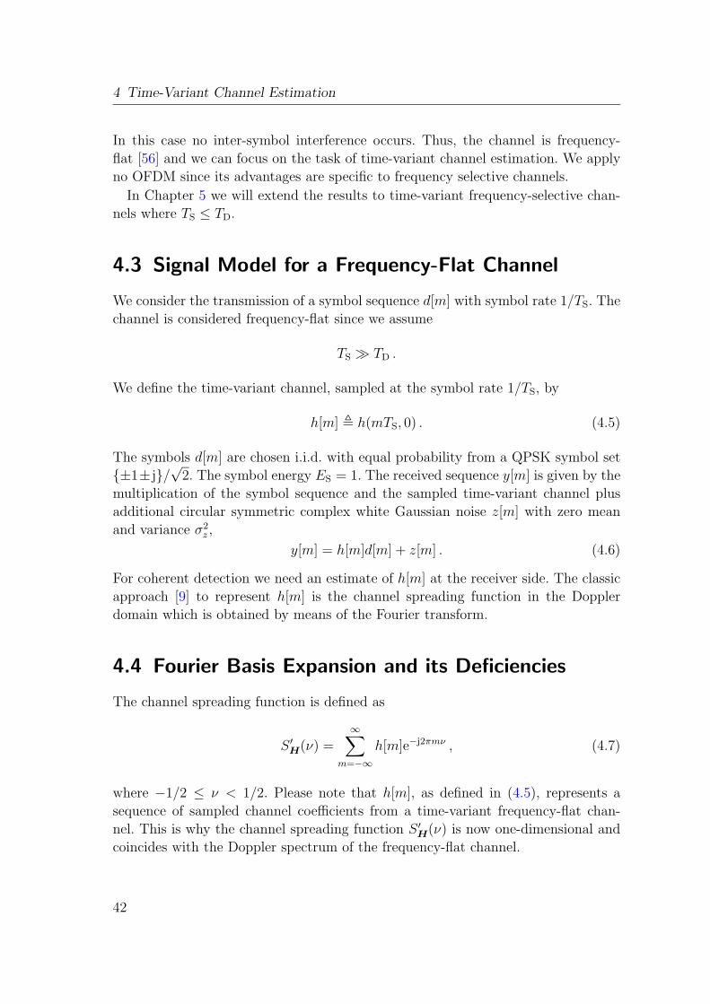
4 Time-Variant Channel Estimation
In this case no inter-symbol interference occurs. Thus, the channel is frequency-
flat [56] and we can focus on the task of time-variant channel estimation. We apply
no OFDM since its advantages are specific to frequency selective channels.
In Chapter 5 we will extend the results to time-variant frequency-selective chan-
nels where TS ≤ TD.
4.3 Signal Model for a Frequency-Flat Channel
We consider the transmission of a symbol sequence d[m] with symbol rate 1/TS. The
channel is considered frequency-flat since we assume
TS À TD .
We define the time-variant channel, sampled at the symbol rate 1/TS, by
h[m] , h(mTS, 0) . (4.5)
The symbols d[m] are chosen i.i.d. with equal probability from a QPSK symbol set
{±1± j}/√
2. The symbol energy ES = 1. The received sequence y[m] is given by the
multiplication of the symbol sequence and the sampled time-variant channel plus
additional circular symmetric complex white Gaussian noise z[m] with zero mean
and variance σ2z ,
y[m] = h[m]d[m] + z[m] . (4.6)
For coherent detection we need an estimate of h[m] at the receiver side. The classic
approach [9] to represent h[m] is the channel spreading function in the Doppler
domain which is obtained by means of the Fourier transform.
4.4 Fourier Basis Expansion and its Deficiencies
The channel spreading function is defined as
S ′H(ν) =
∞∑
m=−∞
h[m]e−j2πmν , (4.7)
where −1/2 ≤ ν < 1/2. Please note that h[m], as defined in (4.5), represents a
sequence of sampled channel coefficients from a time-variant frequency-flat chan-
nel. This is why the channel spreading function S ′H(ν) is now one-dimensional and
coincides with the Doppler spectrum of the frequency-flat channel.
42

4.4 Fourier Basis Expansion and its Deficiencies
For a wireless system the maximum normalized Doppler bandwidth νDmax is
known so that S ′H(ν) is bandlimited, and vanishes for |ν| > νDmax. This can be
expressed by
h[m] =
νDmax∫
−νDmax
S ′H(ν)ej2πmνd ν . (4.8)
In order to enable block based processing we limit the observation time to m ∈{0, . . . ,M − 1} which results in rectangular windowing of h[m], thus
SH(ν) =M−1∑
m=0
h[m]e−j2πmν . (4.9)
We are able to represent h[m] for m ∈ {0, . . . ,M − 1} uniquely by sampling in the
frequency-domain
SH[d] =M−1∑
m=0
h[m]e−j2πmd/M = SH(d/M), (4.10)
for d ∈ {−M/2, . . . ,M/2 − 1} and M even, a representation well-known as DFT.
The rectangular windowing in (4.10) results in spectral leakage [55, Sec. 5.4] [53,
Sec. 3.7]. This means, the energy from low frequency Fourier coefficients leaks to
the full frequency range. Therefore, the support region of SH[d] is not limited to
|d| ≤ dνDmaxMe. However, SH[d] will decay with increasing |d|.
4.4.1 Numerical Example
Figure 4.2 illustrates the spectral leakage effect by plotting the magnitude of the
sampled channel-spreading function SH[d] (and an interpolated version SH(ν))
which arises in an actual communication system after time windowing to m ∈{0, . . . ,M − 1}. For comparison the channel spreading function without windowing
S ′H(ν) is shown too. We consider a transmission with carrier frequency fC = 2 GHz
at a symbol rate 1/TS = 48.6 · 103 s−1. The data block has length of M = 256
symbols. These parameters match the one of the MC-CDMA system defined in Sec-
tion 3.1.1. The maximum speed of the user vmax = 102.5 km/h which results in a
maximum normalized Doppler frequency νDmax = 3.9 · 10−3. We assume a dense
scattering environment. The system parameters result in a time-bandwidth product
νDmaxM = 1.
Figure 4.3 shows the difference between the energy in the index set {−U, . . . , U}and the total energy for varying U which is identical to the mean square error
MSE =U∑
d=−U
|SH[d]|2 −M/2−1∑
d=−M/2
|SH[d]|2 , (4.11)
43
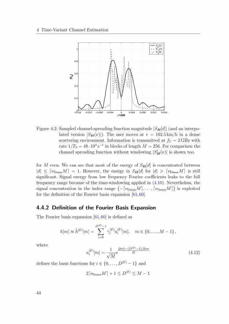
4 Time-Variant Channel Estimation
−0.016 −0.012 −0.008 −0.004 0 0.004 0.008 0.012 0.0160
0.2
0.4
0.6
0.8
1
ν=d/M
|SH
|
SH(ν)
S’H(ν)
SH[d]
Figure 4.2: Sampled channel-spreading function magnitude |SH[d]| (and an interpo-
lated version |SH(ν)|). The user moves at v = 102.5 km/h in a dense
scattering environment. Information is transmitted at fC = 2 GHz with
rate 1/TS = 48 ·103 s−1 in blocks of length M = 256. For comparison the
channel spreading function without windowing |S ′H(ν)| is shown too.
for M even. We can see that most of the energy of SH[d] is concentrated between
|d| ≤ dνDmaxMe = 1. However, the energy in SH[d] for |d| > dνDmaxMe is still
significant. Signal energy from low frequency Fourier coefficients leaks to the full
frequency range because of the time-windowing applied in (4.10). Nevertheless, the
signal concentration in the index range {−dνDmaxMe, . . . , dνDmaxMe} is exploited
for the definition of the Fourier basis expansion [61,60].
4.4.2 Definition of the Fourier Basis Expansion
The Fourier basis expansion [61,60] is defined as
h[m] ≈ h(F)[m] =D(F)−1∑
i=0
γ(F)i u
(F)i [m], m ∈ {0, . . . ,M − 1} ,
where
u(F)i [m] =
1√M
ej2π(i−(D(F)−1)/2)m
M (4.12)
defines the basis functions for i ∈ {0, . . . , D(F) − 1} and
2dνDmaxMe + 1 ≤ D(F) ≤ M − 1
44

4.4 Fourier Basis Expansion and its Deficiencies
0 1 2 3 4 5 6 7 8 9 10 1110
−2
10−1
100
U
MS
E
Figure 4.3: Mean square error caused by limiting SH[d] to |d| ≤ U .
defines the dimension of the basis expansion.
Wherever possible we will use a generic notation for the basis expansion quantities
ui[m], D, γi, and h[m] to indicate that the expression is applicable to any set of
orthonormal basis functions ui[m]. If we want to specifically reference the Fourier
basis expansion we use the superscript (·)(F).
By choosing D we can control the mean square error of the Fourier basis expansion
that is defined as
MSEM =1
M
M−1∑
m=0
E
{∣∣∣h[m] − h[m]
∣∣∣
2}
. (4.13)
The basis expansion parameters are calculated according to
γi =M−1∑
m=0
h[m]ui∗[m], i ∈ {0, . . . , D − 1} . (4.14)
However, equation (4.14) is of limited practical relevance, because at the receiver
side the channel coefficients h[m] will be available in the form of noisy observations.
Furthermore, observations of the channel can be only obtained at index positions
where known pilots are transmitted. These pilot positions are a subset of {0, . . . ,M−1}.
We will treat all these issues throughout the remainder of this chapter. For now
let us assume that we know the channel h[m] and that the channel is defined by one
propagation path only. Using this most simple channel we analyze the mean square
error of the Fourier basis expansion for D < M in the following section.
45
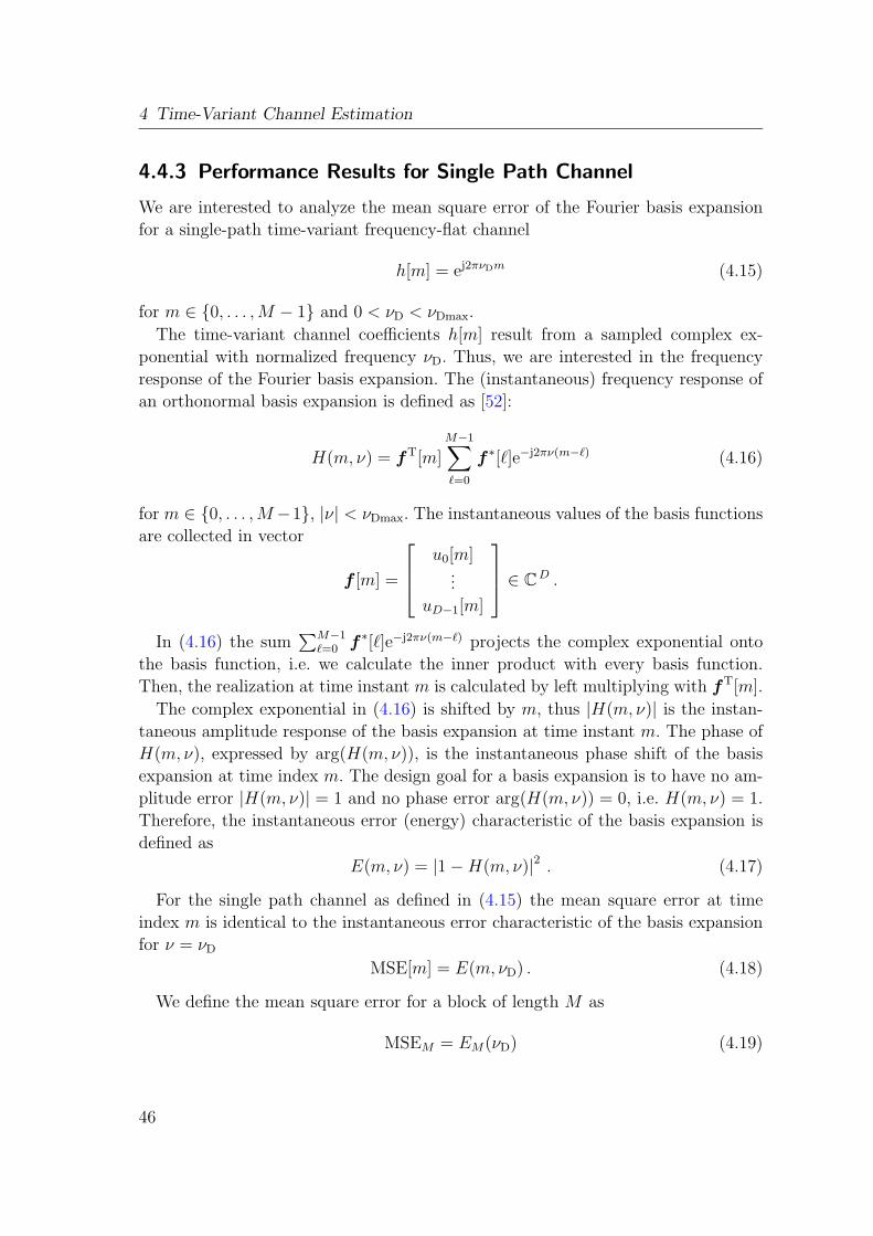
4 Time-Variant Channel Estimation
4.4.3 Performance Results for Single Path Channel
We are interested to analyze the mean square error of the Fourier basis expansion
for a single-path time-variant frequency-flat channel
h[m] = ej2πνDm (4.15)
for m ∈ {0, . . . ,M − 1} and 0 < νD < νDmax.
The time-variant channel coefficients h[m] result from a sampled complex ex-
ponential with normalized frequency νD. Thus, we are interested in the frequency
response of the Fourier basis expansion. The (instantaneous) frequency response of
an orthonormal basis expansion is defined as [52]:
H(m, ν) = fT[m]M−1∑
`=0
f ∗[`]e−j2πν(m−`) (4.16)
for m ∈ {0, . . . ,M −1}, |ν| < νDmax. The instantaneous values of the basis functions
are collected in vector
f [m] =
u0[m]...
uD−1[m]
∈ C
D .
In (4.16) the sum∑M−1
`=0 f ∗[`]e−j2πν(m−`) projects the complex exponential onto
the basis function, i.e. we calculate the inner product with every basis function.
Then, the realization at time instant m is calculated by left multiplying with fT[m].
The complex exponential in (4.16) is shifted by m, thus |H(m, ν)| is the instan-
taneous amplitude response of the basis expansion at time instant m. The phase of
H(m, ν), expressed by arg(H(m, ν)), is the instantaneous phase shift of the basis
expansion at time index m. The design goal for a basis expansion is to have no am-
plitude error |H(m, ν)| = 1 and no phase error arg(H(m, ν)) = 0, i.e. H(m, ν) = 1.
Therefore, the instantaneous error (energy) characteristic of the basis expansion is
defined as
E(m, ν) = |1 − H(m, ν)|2 . (4.17)
For the single path channel as defined in (4.15) the mean square error at time
index m is identical to the instantaneous error characteristic of the basis expansion
for ν = νD
MSE[m] = E(m, νD) . (4.18)
We define the mean square error for a block of length M as
MSEM = EM(νD) (4.19)
46
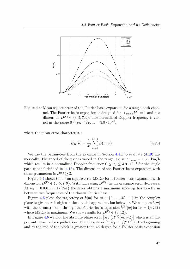
4.4 Fourier Basis Expansion and its Deficiencies
0 0.5 1 1.5 2 2.5 3 3.5
x 10−3
0
0.05
0.1M
SE M
ν (normalized Doppler)
D=3D=5D=7D=9
Figure 4.4: Mean square error of the Fourier basis expansion for a single path chan-
nel. The Fourier basis expansion is designed for dνDmaxMe = 1 and has
dimension D(F) ∈ {3, 5, 7, 9}. The normalized Doppler frequency is var-
ied in the range 0 ≤ νD ≤ νDmax = 3.9 · 10−3.
where the mean error characteristic
EM(ν) =1
M
M−1∑
m=0
E(m, ν) . (4.20)
We use the parameters from the example in Section 4.4.1 to evaluate (4.19) nu-
merically. The speed of the user is varied in the range 0 < v < vmax = 102.5 km/h
which results in a normalized Doppler frequency 0 ≤ νD ≤ 3.9 · 10−3 for the single
path channel defined in (4.15). The dimension of the Fourier basis expansion with
these parameters is D(F) ≥ 3.
Figure 4.4 shows the mean square error MSEM for a Fourier basis expansion with
dimension D(F) ∈ {3, 5, 7, 9}. With increasing D(F) the mean square error decreases.
At νD = 0.0018 = 1/(2M) the error obtains a maximum since νD lies exactly in
between two frequencies of the chosen Fourier base.
Figure 4.5 plots the trajectory of h[m] for m ∈ {0, . . . ,M − 1} in the complex
plane to give more insights in the detailed approximation behavior. We compare h[m]
with the reconstruction through the Fourier basis expansion h(F)[m] for νD = 1/(2M)
where MSEM is maximum. We show results for D(F) ∈ {3, 12}.In Figure 4.6 we plot the absolute phase error
∣∣arg
(H(F)(m, νD)
)∣∣ which is an im-
portant measure for equalization. The phase error for νD = 1/(2M) at the beginning
and at the end of the block is greater than 45 degree for a Fourier basis expansion
47

4 Time-Variant Channel Estimation
−1 −0.5 0 0.5 1−0.5
0
0.5
1
1.5
real(h[m])
imag
(h[m
])
h[m]approximation with D=3approximation with D=12
m m
m
Figure 4.5: Trajectory of h[m] and its approximation by the Fourier basis ex-
pansion h(F)[m]. The trajectories are plotted for discrete index val-
ues m ∈ {0, . . . ,M − 1}. The Fourier basis expansion has dimension
D(F) ∈ {3, 12}, is designed for dνDmaxMe = 1, and is evaluated for a
complex exponential with νD = 1/(2M).
50 100 150 200 2500
10
20
30
40
50
60
70
80
90
m (discrete time)
|pha
se e
rror
|
D=3D=12
Figure 4.6: Absolute phase error∣∣arg
(H(F)(m, νD)
)∣∣ for m ∈ {0, . . . ,M − 1}. The
Fourier basis expansion has dimension D(F) ∈ {3, 12}, is designed for
dνDmaxMe = 1, and is evaluated for a complex exponential with νD =
1/(2M).
48

4.4 Fourier Basis Expansion and its Deficiencies
50 100 150 200 2500
0.1
0.2
0.3
0.4
0.5
0.6
0.7
0.8
0.9
1
m (discrete time)
|am
plitu
de e
rror
|
D=3D=12
Figure 4.7: Absolute amplitude error∣∣1 −
∣∣H(F)(m, νD)
∣∣∣∣ for m ∈ {0, . . . ,M − 1}.
The Fourier basis expansion has dimension D(F) ∈ {3, 12}, is designed
for dνDmaxMe = 1, and is evaluated for a complex exponential with
νD = 1/(2M).
with a dimension of D(F) ∈ {3, 12}. With increasing D(F) the phase error at both
ends of the interval decays faster but the initial value stays the same. A symbol
alphabet, like QPSK, that encodes information in the phase is sensible to phase er-
rors in the channel estimation. Thus, decision errors will result from the phase error
inherent to the Fourier basis expansion leading to an error floor at higher signal to
noise ratios.
Figure 4.7 plots the absolute amplitude error∣∣∣1 −
∣∣H(F)(m, νD)
∣∣
∣∣∣
for νD = 1/(2M). The behavior depicted in Figure 4.6 and Figure 4.7 is similar
to the well-known Gibbs phenomenon [55, Sec. 8.2.2]. If the DFT is truncated at
dνDmaxMe the Gibbs effect together with spectral leakage leads to significant phase
and amplitude errors at the beginning and at the end of the data block. These
(deterministic) errors will result in an error floor at higher signal to noise ratios
for a single-user detector if the Fourier basis expansion is used for time-variant
channel equalization as was shown in [8] and by the author in [88]. We can conclude
that the dimension of the Fourier basis expansion 2dνDmaxMe + 1 that is reported
in [61, 60, 4, 42, 47] is not sufficient for error free detection. In Section 5 we will
analyze the effect of the Fourier basis expansion in the context of multi-user detection
algorithms.
49

4 Time-Variant Channel Estimation
The analysis in this section shows clearly that the Fourier basis expansion has
several drawbacks and a different set of better suited basis functions must be found.
The theory of time-concentrated and bandlimited sequences developed by Slepian
[69] enables a new approach for the time-variant channel estimation problem which
we will pursue in the next section.
4.5 Slepian Basis Expansion
Slepian [69] asked which sequences are bandlimited to the frequency range
[−νDmax, νDmax] and simultaneously most concentrated in a certain time interval
of length M . The associated optimization problem was solved first for continuous
time in [70] and later for discrete time in [69]. In both cases Slepian found that
the desired set of orthogonal sequence are the eigenfunctions of an integral operator
and simultaneously of a commuting differential operator [71]. These special results
enable the numerical calculation for practical applications.
We are interested in the discrete time case. The sequences u[m] we are seeking
shall have their maximum energy concentration in an interval with length M
λ =
M−1∑
m=0
|u[m]|2
∞∑
m=−∞
|u[m]|2, (4.21)
while being bandlimited to νDmax, hence
u[m] =
νDmax∫
−νDmax
U(ν)ej2πmνd ν (4.22)
where
U(ν) =∞∑
m=−∞
u[m]e−j2πmν . (4.23)
We see that 0 ≤ λ ≤ 1.
The solutions of this constrained maximization problem are the discrete prolate
spheroidal (DPS) sequences [69]. The DPS sequences u(S)i [m, νDmax,M ] are defined
as the real solution of
M−1∑
`=0
sin(2πνDmax(` − m))
π(` − m)u
(S)i [`, νDmax,M ] = λi(νDmax,M)u
(S)i [m, νDmax,M ] (4.24)
50
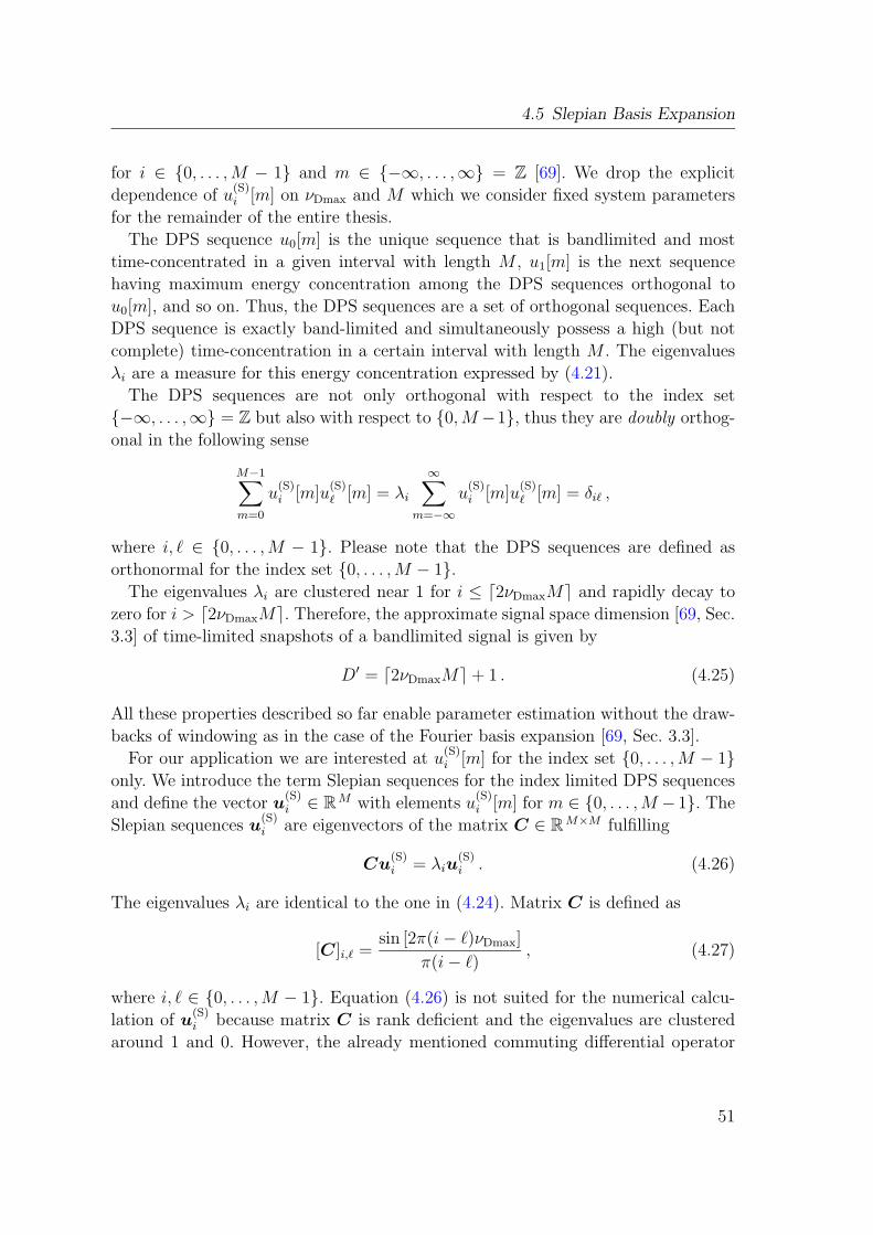
4.5 Slepian Basis Expansion
for i ∈ {0, . . . ,M − 1} and m ∈ {−∞, . . . ,∞} = Z [69]. We drop the explicit
dependence of u(S)i [m] on νDmax and M which we consider fixed system parameters
for the remainder of the entire thesis.
The DPS sequence u0[m] is the unique sequence that is bandlimited and most
time-concentrated in a given interval with length M , u1[m] is the next sequence
having maximum energy concentration among the DPS sequences orthogonal to
u0[m], and so on. Thus, the DPS sequences are a set of orthogonal sequences. Each
DPS sequence is exactly band-limited and simultaneously possess a high (but not
complete) time-concentration in a certain interval with length M . The eigenvalues
λi are a measure for this energy concentration expressed by (4.21).
The DPS sequences are not only orthogonal with respect to the index set
{−∞, . . . ,∞} = Z but also with respect to {0,M −1}, thus they are doubly orthog-
onal in the following sense
M−1∑
m=0
u(S)i [m]u
(S)` [m] = λi
∞∑
m=−∞
u(S)i [m]u
(S)` [m] = δi` ,
where i, ` ∈ {0, . . . ,M − 1}. Please note that the DPS sequences are defined as
orthonormal for the index set {0, . . . ,M − 1}.The eigenvalues λi are clustered near 1 for i ≤ d2νDmaxMe and rapidly decay to
zero for i > d2νDmaxMe. Therefore, the approximate signal space dimension [69, Sec.
3.3] of time-limited snapshots of a bandlimited signal is given by
D′ = d2νDmaxMe + 1 . (4.25)
All these properties described so far enable parameter estimation without the draw-
backs of windowing as in the case of the Fourier basis expansion [69, Sec. 3.3].
For our application we are interested at u(S)i [m] for the index set {0, . . . ,M − 1}
only. We introduce the term Slepian sequences for the index limited DPS sequences
and define the vector u(S)i ∈ R
M with elements u(S)i [m] for m ∈ {0, . . . ,M − 1}. The
Slepian sequences u(S)i are eigenvectors of the matrix C ∈ R
M×M fulfilling
Cu(S)i = λiu
(S)i . (4.26)
The eigenvalues λi are identical to the one in (4.24). Matrix C is defined as
[C]i,` =sin [2π(i − `)νDmax]
π(i − `), (4.27)
where i, ` ∈ {0, . . . ,M − 1}. Equation (4.26) is not suited for the numerical calcu-
lation of u(S)i because matrix C is rank deficient and the eigenvalues are clustered
around 1 and 0. However, the already mentioned commuting differential operator
51

4 Time-Variant Channel Estimation
offers an numerically fast and stable way for the calculation of u(S)i . Please refer
to [69] and [53, Section 8.3] for more details on the numerical calculation of the
Slepian sequences. We will come back to the utility of (4.26) later.
Concluding, the Slepian sequences span an orthonormal basis which allows to
represent time-limited snapshots of bandlimited sequences through a basis expan-
sion. The Slepian basis expansion expands the sequence h[m] in terms of Slepian
sequences u(S)i [m]
h[m] ≈ h(S)[m] =D(S)−1∑
i=0
u(S)i [m]γ
(S)i , (4.28)
where m ∈ {0, . . . ,M − 1}. The dimension of this basis expansion fulfills
D′ ≤ D(S) ≤ M .
By choosing D(S) we can control the mean square error defined in (4.13).
In order to highlight the utility of the Slepian basis expansion in terms of di-
mension reduction we give a numerical example of an actual communication sys-
tem. Again, we use the parameters from Section 4.4.1 that are: carrier frequency
fC = 2 GHz, symbol rate 1/TS = 48.6 · 103 s−1, maximum speed of the user
vmax = 102.5 km/h, maximum normalized Doppler frequency νDmax = 3.9 · 10−3,
and data block length M = 256. With these system parameters the approximate
dimension of the signal space D′ = d2νDmaxMe+ 1 = 3. Therefore, the dimension of
the estimation problem is reduced by a factor of 256/3 = 85 which is a very consider-
able saving. In Figure 4.8 the DPS eigenvalue spectrum is given. The corresponding
Slepian sequences ui for i ∈ {0, . . . , 4} are depicted in Figure 4.9.
4.5.1 Parameter Estimation From Noisy Observations
We insert the basis expansion (4.28) in the signal model (4.6),
y[m] = h[m]d[m] + z[m] =
(D−1∑
i=0
ui[m]γi
)
d[m] + z[m] . (4.29)
Hence, we can visualize the communication system as depicted in Figure 4.10. The
transmission takes place over D parallel channels with fixed complex attenuation γi
followed by modulation with the orthonormal sequences ui[m].
For now we assume that the receiver has knowledge of all transmitted data symbols
in a data block, which is typically the case in iterative receiver structures. Since the
data symbols have constant modulus |d[m]| =√
ES = 1 we obtain a noisy estimate
of the instantaneous channel values through
h[m] = y[m]d∗[m] = h[m] + z[m]d∗[m] .
52
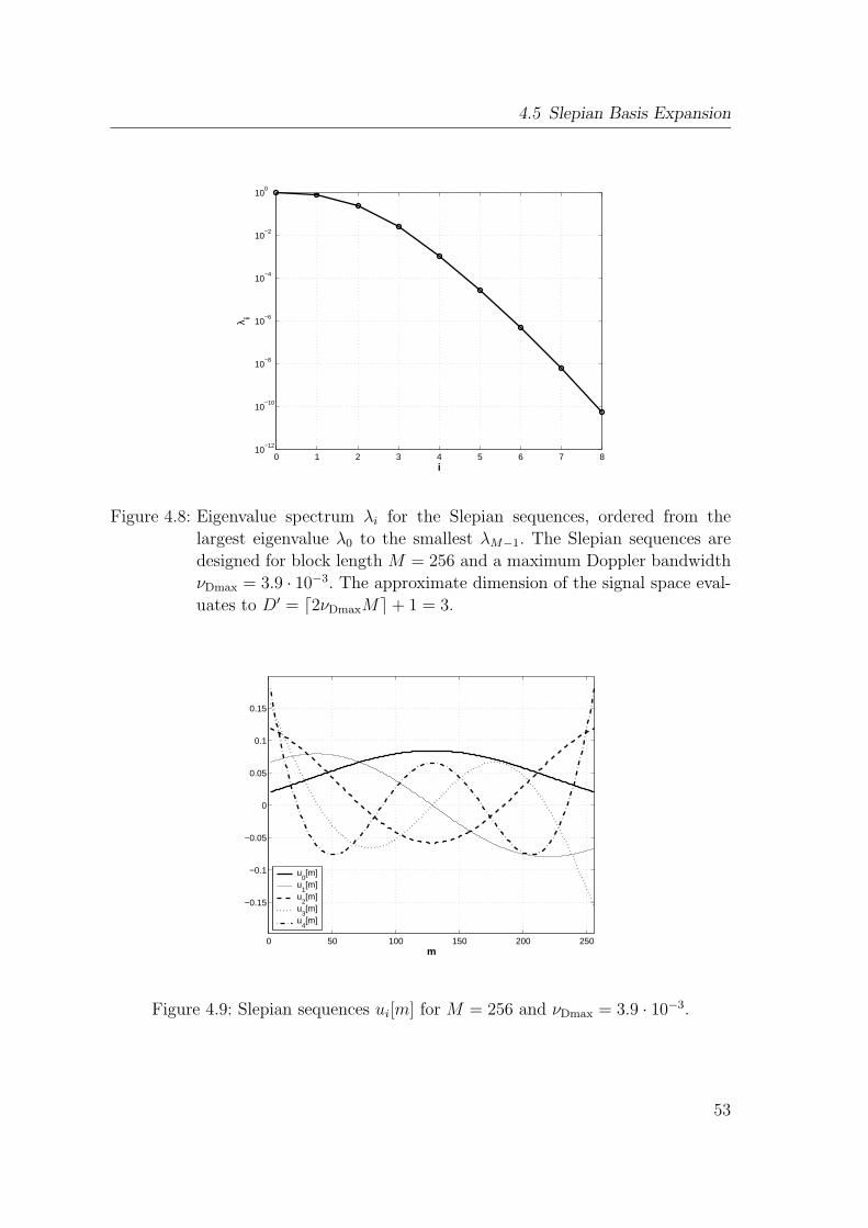
4.5 Slepian Basis Expansion
0 1 2 3 4 5 6 7 810
−12
10−10
10−8
10−6
10−4
10−2
100
i
λ i
Figure 4.8: Eigenvalue spectrum λi for the Slepian sequences, ordered from the
largest eigenvalue λ0 to the smallest λM−1. The Slepian sequences are
designed for block length M = 256 and a maximum Doppler bandwidth
νDmax = 3.9 · 10−3. The approximate dimension of the signal space eval-
uates to D′ = d2νDmaxMe + 1 = 3.
0 50 100 150 200 250
−0.15
−0.1
−0.05
0
0.05
0.1
0.15
m
u0[m]
u1[m]
u2[m]
u3[m]
u4[m]
Figure 4.9: Slepian sequences ui[m] for M = 256 and νDmax = 3.9 · 10−3.
53

4 Time-Variant Channel Estimation
uD−1[m]
u0[m]
...
u2[m]
γ1
...
γD−1
d[m]
γ0
y[m]
z[m]
Figure 4.10: Representation of a linear time-variant frequency-flat channel h[m]
using time-invariant weighting coefficients γi and modulation with
orthonormal basis functions ui[m]. This model is valid for m ∈{0, . . . ,M − 1}.
Considering the model in Figure 4.10 we can estimate the unknown coefficients in
(4.28) through
γi =M−1∑
m=0
h[m]u∗i [m] =
M−1∑
m=0
y[m]d∗[m]u∗i [m] (4.30)
for i ∈ {0, . . . , D(S) − 1}.The mean square error (4.13) of the basis expansion can be described by the sum
of a square bias and a variance term
MSEM = bias2M + varM . (4.31)
We will see in the next section that bias2M is depending on the actual set of basis
functions and varM depends linearly on the noise variance σ2z and the dimension D
of the basis expansion.
4.5.2 Analytic Performance Results
For the purposes of performance analysis for a nominal ensemble of channel real-
izations of h[m], let us specify a Doppler power spectral density
Shh(ν) =∞∑
m=−∞
Rhh[m]e−j2πmν ,
where the autocorrelation is defined as
Rhh[m] = E{h∗[m + m]h[m]} . (4.32)
54

4.5 Slepian Basis Expansion
The square bias of the basis expansion can be expressed [52] by integrating the
single path error expression (4.18) over the Doppler power spectrum,
bias2[m] =
12∫
− 12
E(m, ν)Shh(ν)d ν . (4.33)
The square bias for a block of length M is defined as
bias2M ,
1
M
M−1∑
m=0
bias2[m] =
12∫
− 12
EM(ν)Shh(ν)d ν , (4.34)
where the mean error characteristic (4.20)
EM(ν) =1
M
M−1∑
m=0
E(m, ν) . (4.35)
The bias2M is defined as the mean square error (4.31) in the absence of noise (σ2
z = 0),
see also [66, Sec. 9.9].
The parameter estimation in (4.30) is operating with noisy observations. As al-
ready stated, the biased part of the mean square error (4.13) is independent of the
noise variance. The variance expression for the basis expansion is given as [52, Sec.
6.1.4]
var[m] ≈ σ2zf
H[m]f [m] . (4.36)
This equation becomes exact for bias2[m] = 0. The mean variance for block length
M is given by
varM =1
M
M−1∑
m=0
var[m] = σ2z
D
M. (4.37)
Equation (4.37) clearly shows that the variance is independent of the used set of
orthonormal basis functions and increases linearly with the dimension of the basis
expansion D and the noise variance σ2z [52].
The approximate dimension of the signal space D′ (4.25) becomes a tight bound
for large M (and exact for M → ∞). By insertion of D′ into (4.37)
var(S)M = σ2
z
d2νDmaxMe + 1
M
we are able to obtain a lower tight bound for var(S)M in the limit
limM→∞
var(S)M ≥ 2νDmaxσ
2z .
55
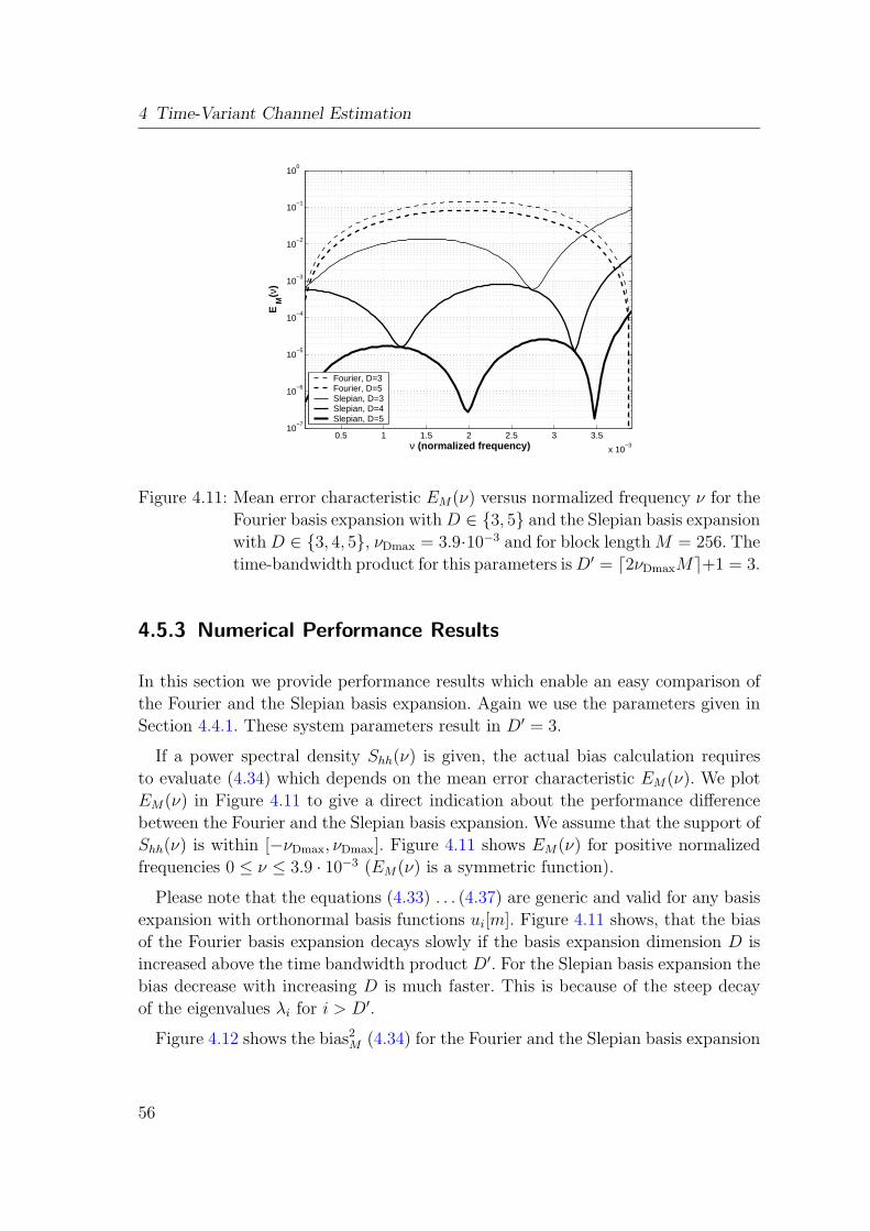
4 Time-Variant Channel Estimation
0.5 1 1.5 2 2.5 3 3.5
x 10−3
10−7
10−6
10−5
10−4
10−3
10−2
10−1
100
ν (normalized frequency)
E M
(ν)
Fourier, D=3Fourier, D=5Slepian, D=3Slepian, D=4Slepian, D=5
Figure 4.11: Mean error characteristic EM(ν) versus normalized frequency ν for the
Fourier basis expansion with D ∈ {3, 5} and the Slepian basis expansion
with D ∈ {3, 4, 5}, νDmax = 3.9·10−3 and for block length M = 256. The
time-bandwidth product for this parameters is D′ = d2νDmaxMe+1 = 3.
4.5.3 Numerical Performance Results
In this section we provide performance results which enable an easy comparison of
the Fourier and the Slepian basis expansion. Again we use the parameters given in
Section 4.4.1. These system parameters result in D′ = 3.
If a power spectral density Shh(ν) is given, the actual bias calculation requires
to evaluate (4.34) which depends on the mean error characteristic EM(ν). We plot
EM(ν) in Figure 4.11 to give a direct indication about the performance difference
between the Fourier and the Slepian basis expansion. We assume that the support of
Shh(ν) is within [−νDmax, νDmax]. Figure 4.11 shows EM(ν) for positive normalized
frequencies 0 ≤ ν ≤ 3.9 · 10−3 (EM(ν) is a symmetric function).
Please note that the equations (4.33) . . . (4.37) are generic and valid for any basis
expansion with orthonormal basis functions ui[m]. Figure 4.11 shows, that the bias
of the Fourier basis expansion decays slowly if the basis expansion dimension D is
increased above the time bandwidth product D′. For the Slepian basis expansion the
bias decrease with increasing D is much faster. This is because of the steep decay
of the eigenvalues λi for i > D′.
Figure 4.12 shows the bias2M (4.34) for the Fourier and the Slepian basis expansion
56

4.5 Slepian Basis Expansion
0.5 1 1.5 2 2.5 3 3.5
x 10−3
10−4
10−3
10−2
10−1
100
νD
(normalized Doppler)
bias
2 M
FourierSlepian
Figure 4.12: Comparison of bias2M for the Slepian and the Fourier basis expansion.
We use a Jakes’ Doppler spectrum and vary the Doppler bandwidth in
the range 0 ≤ νD ≤ 3.9 · 10−3 which corresponds to a velocity range
of 0 ≤ v ≤ 102.5 km/h. The basis expansions have dimension D = 3.
The Slepian sequences are designed according to νDmax = 3.9 ·10−3 and
block length M = 256.
when evaluated for the Jakes’ Doppler spectrum
Shh(ν) =
1
πνD
√
1 −(
ννD
)2for |ν| < νD ,
0 otherwise.
(4.38)
We vary the normalized Doppler bandwidth in the range 0 ≤ νD ≤ 3.9 · 10−3
corresponding to a velocity range of 0 ≤ v ≤ 102.5 km/h. The results in Figure 4.12
document that the Slepian basis expansion square bias is one magnitude smaller
than the square bias of the Fourier basis expansion. The mean variance varM (4.37)
is independent of the chosen set of basis functions ui[m] but var[m] (4.36) is not.
Figure 4.13 shows var[m]/σ2z for the Fourier and the Slepian basis expansion.
We emphasize that the selection of a suitable Slepian basis, defined by M and
νDmax, exploits the band-limitation of the Doppler spectrum to νDmax only. The
details of the Doppler spectrum for |ν| < νDmax are irrelevant. The necessary dimen-
sion of the basis expansion for wireless channels at 2 GHz and vehicular velocities
up to 102.5 km/h is in the order of three only. For the calculation of the Slepian
sequences efficient methods exists that avoid the numerical instabilities of the eigen-
57
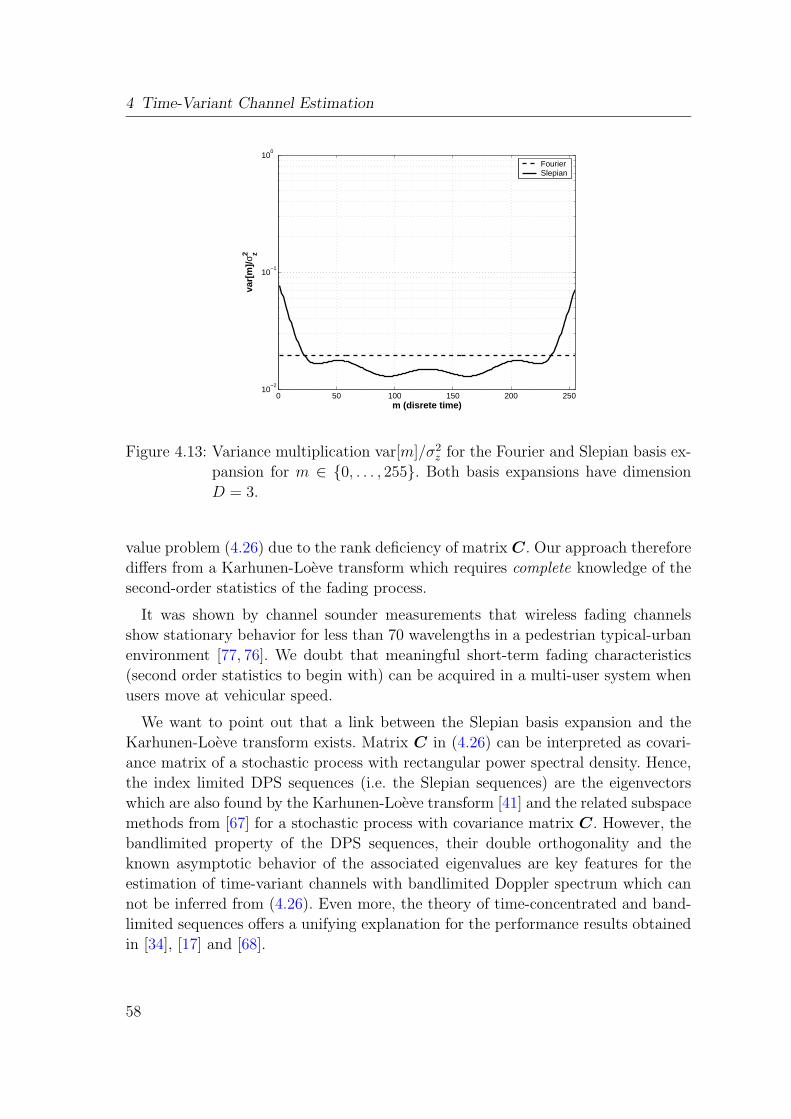
4 Time-Variant Channel Estimation
0 50 100 150 200 25010
−2
10−1
100
m (disrete time)
var[
m]/
σ z2
FourierSlepian
Figure 4.13: Variance multiplication var[m]/σ2z for the Fourier and Slepian basis ex-
pansion for m ∈ {0, . . . , 255}. Both basis expansions have dimension
D = 3.
value problem (4.26) due to the rank deficiency of matrix C. Our approach therefore
differs from a Karhunen-Loeve transform which requires complete knowledge of the
second-order statistics of the fading process.
It was shown by channel sounder measurements that wireless fading channels
show stationary behavior for less than 70 wavelengths in a pedestrian typical-urban
environment [77, 76]. We doubt that meaningful short-term fading characteristics
(second order statistics to begin with) can be acquired in a multi-user system when
users move at vehicular speed.
We want to point out that a link between the Slepian basis expansion and the
Karhunen-Loeve transform exists. Matrix C in (4.26) can be interpreted as covari-
ance matrix of a stochastic process with rectangular power spectral density. Hence,
the index limited DPS sequences (i.e. the Slepian sequences) are the eigenvectors
which are also found by the Karhunen-Loeve transform [41] and the related subspace
methods from [67] for a stochastic process with covariance matrix C. However, the
bandlimited property of the DPS sequences, their double orthogonality and the
known asymptotic behavior of the associated eigenvalues are key features for the
estimation of time-variant channels with bandlimited Doppler spectrum which can
not be inferred from (4.26). Even more, the theory of time-concentrated and band-
limited sequences offers a unifying explanation for the performance results obtained
in [34], [17] and [68].
58

4.6 Pilot Based Channel Estimation
4.6 Pilot Based Channel Estimation
Channel estimation algorithms for the downlink have to be implemented in the
mobile equipment and low complexity is a key requirement because of size and
battery constraints. Thus, decision feedback structures or iterative receivers with
soft-input soft-output decoders are too expensive in terms of resource consumption.
We analyze a pilot based channel estimation scheme for time-variant frequency-flat
channels. This scheme can be easily extended to an OFDM system in time-variant
frequency-selective channels where it is applied on a per-subcarrier basis.
We transmit symbols in blocks of length M . Each block consists of M − J data
symbols b[m] with J interleaved pilot symbols p[m]
d[m] = b[m] + p[m] . (4.39)
The data symbols satisfy
b[m] ∈ {±1 ± j}/√
2 for m /∈ P ,
and
b[m] = 0 for m ∈ P .
The pilot symbols are i.i.d. chosen from the QPSK symbol set
p[m] = {±1 ± j}/√
2 for m ∈ P ,
and
p[m] = 0 for m /∈ P .
The pilot placement is defined through the index set
P =
{⌊
iM
J+
M
2J
⌋
| i ∈ {0, . . . , J − 1}}
. (4.40)
Figure 4.14 shows an example for the pilot set P defined in (4.40). The symbols
have constant modulus, their energy is normalized |d[m]| =√
ES = 1.
m = 14. . .
1272
10
Figure 4.14: Example pilot pattern P = {2, 7, 12} defined by (4.40) for M = 15 and
J = 3.
59

4 Time-Variant Channel Estimation
The basis expansion parameters shall be estimated utilizing the J known pilots
at m ∈ P. We estimate the basis expansion parameters according to:
γi =1
∑
m∈P
|ui[m]|2∑
m∈P
y[m]p∗[m]u∗i [m] , (4.41)
where i ∈ {0, . . . , D − 1}. We use a generic notation since (4.41) is valid for any
basis expansion.
To achieve high spectral efficiency the percentage of pilot symbols in a data block
is required to be as small as possible. We will see in Section 4.8 that the estimator in
(4.41) is biased especially for small values of J . This is true not only for the Fourier
basis expansion but also for the Slepian basis expansion since the orthogonality of
the basis functions is lost. The reason for the lost orthogonality can be seen in (4.41)
where the sum is evaluated on the index position defined by the pilot set P rather
than the complete orthogonality set {0, . . . ,M − 1}.The DPS sequences are bandlimited to [−νDmax, νDmax] and mostly concentrated
on the time index set {0, . . . ,M − 1}. If we would be able to design sequences u′i[m]
that keep these properties but are orthogonal on the pilot set P
∑
m∈P
u′i[m]u′
`[m] = δi,`σ′i2
(4.42)
we can avoid the bias due to the pilot grid while keeping the simple structure of
(4.41).
The derivations of the DPS sequences [69] involve an integral operator for which
no easy way was found to incorporate the constraint (4.42) in a numerical stable way.
Related approaches for generalization of the DPS sequences were pursued in [22] and
[12] in the field of power spectral density estimation. However, the DPS sequences
can be approximated by finite discrete prolate spheroidal (FDPS) sequences which
are doubly orthogonal over two finite index sets [25,95].
We introduce the FDPS sequences in Section 4.7. The derivation of the FDPS
sequences involves matrix operators which we describe in Section 4.7.1. The matrix
operators have a more tractable structure which enables us to incorporate (4.42)
more easily. Finally, we obtain generalized FDPS sequences with an orthogonality
over the pilot set P in Section 4.7.2.
60

4.7 Finite Slepian Basis Expansion
4.7 Finite Slepian Basis Expansion
The finite discrete prolate spheroidal (FDPS) sequences u(FS)i [m] described in [25]
and [95] are orthonormal over the finite index set {0, . . . , aM − 1}, i.e.
aM−1∑
m=0
u(FS)i [m]u
(FS)` [m] = δi` for i, ` ∈ {0, . . . , D(FS) − 1} ,
and orthogonal over the index set {0,M − 1}M−1∑
m=0
u(FS)i [m]u
(FS)` [m] = σ
(FS)i
2δi` for i, ` ∈ {0, . . . , D(FS) − 1} .
We link these two intervals through the integer parameter a > 1, a ∈ Z+. D(FS) is
a certain number D′ ≤ D(FS) defining the dimensionality of the finite Slepian basis
expansion. The approximate dimension of the signal space is given by (4.25)
D′ = d2νDmaxMe + 1 .
The FDPS sequences u(FS)i ∈ R
aM with elements u(FS)i [m] are the left singular
vectors of the matrix C′ ∈ C
aM×M which is defined as
[C′]i,` =1
aM
sin [π(2daνDmaxMe + 1)(i − `)/(aM)]
sin [π(i − `)/(aM)].
The FDPS sequences deviate here from the DPS sequences, since their defining
matrix is non symmetric. Therefore, the eigenvectors do not exist and we have to
resort to the singular value decomposition of matrix C′. The left singular vectors of
the non symmetric matrix C′ can be calculated as the eigenvectors of the product
C′C′H fulfilling [23, Sec. 8.3]
C′C′Hu
(FS)i = σ
(FS)i
2u
(FS)i for i ∈ {0, . . . , D(FS) − 1} . (4.43)
The singular values are denoted by σ(FS)i .
The rank of matrix C′ is given by
rank(C′) = min(2adνDmaxMe + 1,M) , (4.44)
hence (4.44) defines an upper bound for the dimension of the finite Slepian basis
expansion
D′ ≤ D(FS) ≤ min(2adνDmaxMe + 1,M) . (4.45)
In analogy to the previous section we define the finite Slepian sequences as the
vectors u(FS)i ∈ R
M obtained by index limiting the FDPS sequences u(FS)i [m] to
{0, . . . ,M − 1}.
61

4 Time-Variant Channel Estimation
The finite Slepian sequences u(FS)i converge to the Slepian sequences u
(S)i for
a → ∞ [25]
lima→∞
1
σ(FS)i
u(FS)i = u
(S)i , (4.46)
The factor 1/σ(FS)i in (4.46) is due to the fact, that the Slepian sequences are defined
as orthonormal while the DPS sequences are orthogonal [69]. In the finite case the
situation is opposite, the finite Slepian sequences are defined as orthogonal while
the FDPS sequences are orthonormal.
Matrix C′ is a tall matrix with dimension aM × M . In the limit a → ∞ the first
M × M elements of C′ coincide with C
lima→∞
[C′]i,` = [C]i,` for i, ` ∈ {0, . . . ,M − 1} ,
thus matrix C′ has the structure
lima→∞
C′ =
[C
B
]
. (4.47)
The square of the singular values of C′ converge to the eigenvalue of C
lima→∞
σ(FS)i
2= λ
(S)i .
In the case of finite values a > 1 the finite Slepian sequences approximate the
Slepian sequences. We will show by numerical simulation in Section 4.8 that a value
a = 2 is already sufficient for our purposes. Comparing Fig. 4.15 with Fig. 4.9 we
can see that there is hardly any difference for an approximation factor a = 2.
4.7.1 Operator Representation
The defining matrix for the FDPS sequences C′ can be explained as a concatenation
of a time-limiting operator to the discrete index set {0, . . . ,M − 1} and a band-
limiting operator to the frequency range [−νDmax, νDmax]. Later in Section 4.7.2, we
will modify the time-limiting operator for the pilot set P which allows us to obtain
the generalized FDPS sequences.
We define the zero padded matrix
C′=
[C′,0aM×(a−1)M
]∈ R
aM×aM , (4.48)
and the time-limiting operator D′ ∈ R
aM×aM as the diagonal matrix
D′ = diag
([1M
0aM−M
])
. (4.49)
62

4.7 Finite Slepian Basis Expansion
0 50 100 150 200 250−0.2
−0.15
−0.1
−0.05
0
0.05
0.1
0.15
0.2
m
u0[m]/σ
0u
1[m]/σ
1u
2[m]/σ
2u
3[m]/σ
3u
4[m]/σ
4
Figure 4.15: Finite Slepian sequences u(GS)i [m]/σ
(GS)i for block length M = 256, max-
imum normalized Doppler bandwidth νDmax = 3.9 · 10−3, and approxi-
mation factor a = 2.
The band limiting operator B ∈ RaM×aM in the frequency domain is given by the
diagonal matrix
B = diag
1adνDmaxMe+1
0aM−2adνDmaxMe−1
1adνDmaxMe
.
Using these definitions above matrix C′can be expressed by [95]
C′= F H
aMBF aMD′ . (4.50)
The DFT matrix F aM performs the transformation from the time domain in the
frequency domain and back.
The filter operator C′
performs time-limitation to {0, . . . ,M − 1} and band-
limitation to [−νDmax, νDmax]. If we apply the filter operator on a zero padded,
time-limited snapshot of the band-limited sequence of channel values
h = [h[0], . . . , h[M − 1]]T ∈ CM (4.51)
they remain (practically) unchanged for the the index range {0, . . . ,M − 1}.[
h
h′
]
≈ C′[
h
0aM−M
]
(4.52)
Equation (4.52) becomes exact for a → ∞.
63

4 Time-Variant Channel Estimation
The finite Slepian sequences u(FS)i are defined as the first M elements of the
left singular vector of matrix C′, thus they are optimally suited to define the finite
Slepian basis expansion to represent h[m] for m ∈ {0, . . . ,M − 1}.
4.7.2 Generalized Finite Slepian Basis Expansion
As already mentioned we are interested to obtain generalized finite Slepian sequences
that are orthogonal on the pilot set P . The time limiting operator D′ (4.49) defines
the inner orthogonality index set {0, . . . ,M − 1} for the finite Slepian sequences. In
order to change the orthogonality set, we define the indicator vector ρ ∈ RM with
elements
ρ[m] =
{1 m ∈ P,
0 m /∈ P;m ∈ {0, . . . ,M − 1} ,
and modify the time limiting (4.49) operator according to
D = diag
([ρ
0aM−M
])
.
Inserting D in (4.50) provides us with
C = F HaMBF aMD .
Since we know the diagonal structure of D and because of the fact that it multiplies
F HaMBF aM from the right we know that C has the following structure
C =[C,0aM×(a−1)M
]∈ R
aM×aM .
Omitting all zero columns we calculate the left singular vectors of C by solving
the eigenvalue problem of CCH [23, Sec. 8.3]
CCHu
(GS)i = σ
(GS)i
2u
(GS)i for i ∈ {0, . . . , D(GS) − 1}
to obtain the generalized FDPS sequences u(GS)i ∈ R
aM with elements u(GS)i [m].
Figure 4.16 shows the generalized FDPS sequences for block length M = 256,
maximum Doppler bandwidth νDmax = 3.9 · 10−3, approximation factor a = 2, and
J = 30 pilot symbols. The singular values are denoted by σ(GS)i . Figure 4.17 shows
the square singular value spectrum corresponding to the generalized FDPS sequences
in Figure 4.16.
The rank of C defines the upper limit for the dimension of the generalized finite
Slepian basis expansion
D′ ≤ D(GS) ≤ min(2adνDmaxMe + 1,M)
64

4.7 Finite Slepian Basis Expansion
0 50 100 150 200 250 300 350 400 450 500−0.1
−0.08
−0.06
−0.04
−0.02
0
0.02
0.04
0.06
0.08
0.1
m
u0[m]
u1[m]
u2[m]
u3[m]
u4[m]
Figure 4.16: Generalized FDPS sequences u(GS)i [m] for block length M = 256, ap-
proximation factor a = 2, maximum Doppler bandwidth νDmax =
3.9 · 10−3, and J = 30 pilot symbols.
0 1 2 3 410
−2
10−1
100
i
σ i2
Figure 4.17: Square singular value spectrum σ(GS)i
2for the generalized FDPS se-
quences designed for block length M = 256, approximation factor
a = 2, maximum Doppler bandwidth νDmax = 3.9 · 10−3, and J = 30
pilots symbols.
65
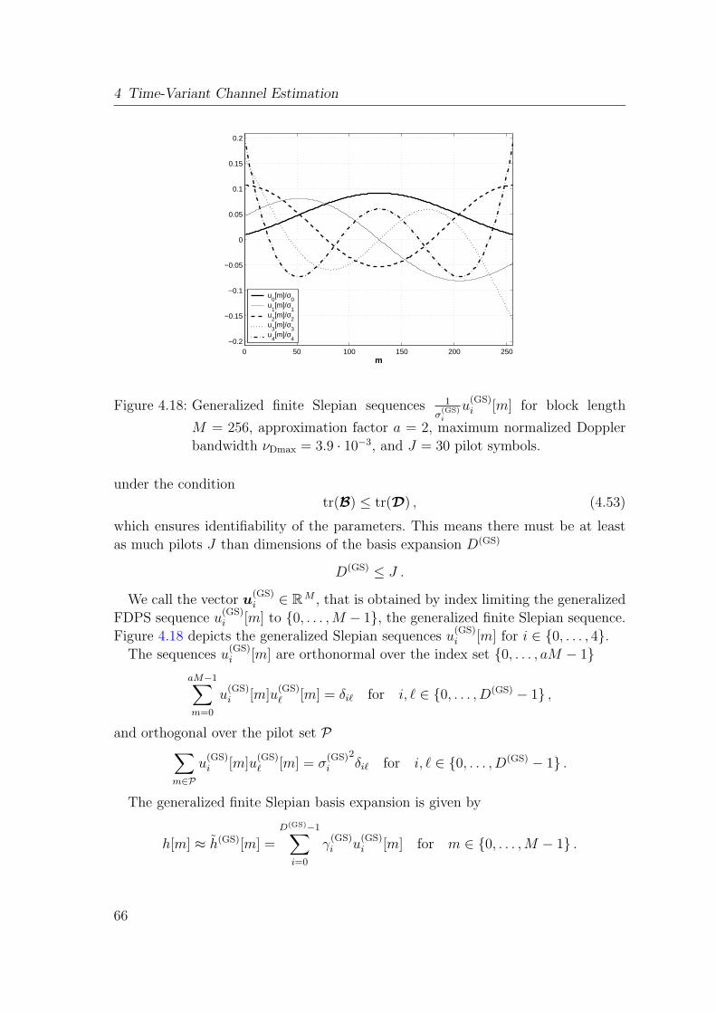
4 Time-Variant Channel Estimation
0 50 100 150 200 250−0.2
−0.15
−0.1
−0.05
0
0.05
0.1
0.15
0.2
m
u0[m]/σ
0u
1[m]/σ
1u
2[m]/σ
2u
3[m]/σ
3u
4[m]/σ
4
Figure 4.18: Generalized finite Slepian sequences 1
σ(GS)i
u(GS)i [m] for block length
M = 256, approximation factor a = 2, maximum normalized Doppler
bandwidth νDmax = 3.9 · 10−3, and J = 30 pilot symbols.
under the condition
tr(B) ≤ tr(D) , (4.53)
which ensures identifiability of the parameters. This means there must be at least
as much pilots J than dimensions of the basis expansion D(GS)
D(GS) ≤ J .
We call the vector u(GS)i ∈ R
M , that is obtained by index limiting the generalized
FDPS sequence u(GS)i [m] to {0, . . . ,M − 1}, the generalized finite Slepian sequence.
Figure 4.18 depicts the generalized Slepian sequences u(GS)i [m] for i ∈ {0, . . . , 4}.
The sequences u(GS)i [m] are orthonormal over the index set {0, . . . , aM − 1}
aM−1∑
m=0
u(GS)i [m]u
(GS)` [m] = δi` for i, ` ∈ {0, . . . , D(GS) − 1} ,
and orthogonal over the pilot set P∑
m∈P
u(GS)i [m]u
(GS)` [m] = σ
(GS)i
2δi` for i, ` ∈ {0, . . . , D(GS) − 1} .
The generalized finite Slepian basis expansion is given by
h[m] ≈ h(GS)[m] =D(GS)−1∑
i=0
γ(GS)i u
(GS)i [m] for m ∈ {0, . . . ,M − 1} .
66
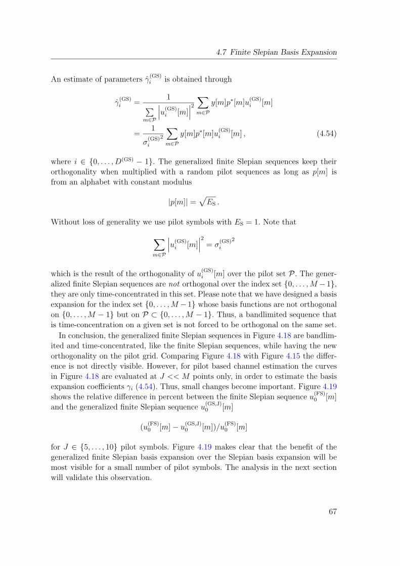
4.7 Finite Slepian Basis Expansion
An estimate of parameters γ(GS)i is obtained through
γ(GS)i =
1∑
m∈P
∣∣∣u
(GS)i [m]
∣∣∣
2
∑
m∈P
y[m]p∗[m]u(GS)i [m]
=1
σ(GS)i
2
∑
m∈P
y[m]p∗[m]u(GS)i [m] , (4.54)
where i ∈ {0, . . . , D(GS) − 1}. The generalized finite Slepian sequences keep their
orthogonality when multiplied with a random pilot sequences as long as p[m] is
from an alphabet with constant modulus
|p[m]| =√
ES .
Without loss of generality we use pilot symbols with ES = 1. Note that
∑
m∈P
∣∣∣u
(GS)i [m]
∣∣∣
2
= σ(GS)i
2
which is the result of the orthogonality of u(GS)i [m] over the pilot set P . The gener-
alized finite Slepian sequences are not orthogonal over the index set {0, . . . ,M −1},they are only time-concentrated in this set. Please note that we have designed a basis
expansion for the index set {0, . . . ,M −1} whose basis functions are not orthogonal
on {0, . . . ,M − 1} but on P ⊂ {0, . . . ,M − 1}. Thus, a bandlimited sequence that
is time-concentration on a given set is not forced to be orthogonal on the same set.
In conclusion, the generalized finite Slepian sequences in Figure 4.18 are bandlim-
ited and time-concentrated, like the finite Slepian sequences, while having the new
orthogonality on the pilot grid. Comparing Figure 4.18 with Figure 4.15 the differ-
ence is not directly visible. However, for pilot based channel estimation the curves
in Figure 4.18 are evaluated at J << M points only, in order to estimate the basis
expansion coefficients γi (4.54). Thus, small changes become important. Figure 4.19
shows the relative difference in percent between the finite Slepian sequence u(FS)0 [m]
and the generalized finite Slepian sequence u(GS,J)0 [m]
(u(FS)0 [m] − u
(GS,J)0 [m])/u
(FS)0 [m]
for J ∈ {5, . . . , 10} pilot symbols. Figure 4.19 makes clear that the benefit of the
generalized finite Slepian basis expansion over the Slepian basis expansion will be
most visible for a small number of pilot symbols. The analysis in the next section
will validate this observation.
67
4 Time-Variant Channel Estimation
0 50 100 150 200 250
−50
−40
−30
−20
−10
0
10
m
%
J=5J=6J=7J=8J=9J=10
Figure 4.19: Relative difference (u(FS)0 [m] − u
(GS,J)0 [m])/u
(FS)0 [m] in percent between
the finite Slepian sequence u(FS)0 [m] and the generalized finite Slepian
sequence u(GS,J)0 [m] for J ∈ {5, . . . , 10} pilot symbols.
4.8 Basis Expansion Error Analysis for Pilot Based
Channel Estimation
In order to demonstrate the merits of the generalized finite Slepian basis expansion
and the Slepian basis expansion, we compare their performance to the Fourier basis
expansion by means of simulations with the system defined in (4.6). Additionally
we will compare the simulation results with analytic results that are derived in the
following Section 4.8.1 and Section 4.8.2.
4.8.1 Basis Expansion Bias
We develop an analytic expression for the basis expansion bias for pilot based channel
estimation extending Niedzwiecki’s results [52, Sec. 6]. We use a generic notation,
the results are applicable to all basis expansions presented so far.
We modify the instantaneous frequency response of a basis expansion (4.16) from
Section 4.15 for the pilot based case and define
H(m, ν) = fT[m]G−1∑
`∈P
f ∗[`]e−j2πν(m−`) , (4.55)
where m ∈ {0, . . . ,M − 1}, |ν| < 1/2 and the diagonal correlation matrix is defined
68

4.8 Basis Expansion Error Analysis for Pilot Based Channel Estimation
as
G = diag ([[G′]0,0, . . . , [G′]D−1,D−1])
with
G′ =∑
`∈P
f [`]fH[`] . (4.56)
We use the diagonal matrix G because we focus on a matched-filter implementation
without the need of a matrix inversion so that we can reduce complexity. If a matrix
inversion is performed, G has to be replaced by G′. The matched filter implemen-
tation of (4.54) is exact for the generalized finite Slepian sequences since they are
orthogonal on the pilot set P ,
G = G′(GS).
For all other basis expansions the estimator in (4.41) results in a small performance
loss.
We repeat here the square bias expressions from Section 4.5.2 for convenience
bias2[m] =
12∫
− 12
E[m, ν]Shh(ν)d ν . (4.57)
with the instantaneous error characteristic E[m, ν] = |1 − H(m, ν)|2 (4.17) and
bias2M =
1
M
M−1∑
m=0
bias2[m] . (4.58)
4.8.2 Basis Expansion Variance
We defineES
N0
=1
σ2z
(4.59)
for channel estimation purposes. Note that this definition is different from Eb/N0
which we use for data detection, cf. (3.9). Based on the results from [52, Sec. 6.1.4]
we can express the basis expansion estimator variance as
var[m] ≈ σ2zf
H[m]G−1f [m] . (4.60)
The mean variance for the complete block of length M is given by
varM ≈ 1
M
M−1∑
m=0
var[m] (4.61)
69

4 Time-Variant Channel Estimation
Equation (4.61) becomes exact for bias2M = 0. For the generalized finite Slepian
basis expansion (4.61) simplifies to
var(GS)M ≈ σ2
z
D
J.
Note that varM increases with decreasing number of pilot symbols J .
4.8.3 Simulation Model and System Assumption
Again, we use the system parameters from Section 4.4.1. We evaluate the time-
variant channel estimator for a channel with autocorrelation
E{h∗[m + m]h[m]} = Rhh[m] = J0(2πνDm) , (4.62)
where J0 is the Bessel function of the first kind and zeroth order. The normalized
one-sided Doppler bandwidth
νD =vfC
c0
TS .
The true speed of the user is denoted by v, with 0 ≤ v < 102.5 km/h. The related
Doppler spectrum is given in (4.38). The range of the normalized Doppler bandwidth
is
0 ≤ νD < νDmax = 3.9 · 10−3 .
The dimension of the Fourier, the Slepian, and the generalized finite Slepian basis
expansion is chosen as D(GS) = D(S) = D(F) = 5. For the generalized finite Slepian
basis expansion we choose an approximation factor of a = 2.
The actual realizations of the time-variant channel h[m] are calculated as the
superposition of 20 impinging waves [93]. See Appendix A for more details.
4.8.4 Analytic Results
We evaluate (4.58) for the Jakes’ spectrum (4.38) and the transmission of J = 10
pilots. Figure 4.20 plots the the square bias of the generalized finite Slepian basis
expansion, the Slepian basis expansion and the Fourier basis expansion for 0 ≤ νD ≤3.9·10−3. The analytic results are denoted ’theor.’. The square bias of the generalized
finite Slepian basis expansion is three magnitudes smaller than the square bias of
the Fourier basis expansion. The square bias of the Fourier basis expansion slightly
decays towards νDmax = 3.9 · 10−3 = 1/M = 1/256 since this frequency coincides
with the one of the Fourier basis function and thus is a local minimum. The same
behavior is also visible in Figure 4.21.
70

4.8 Basis Expansion Error Analysis for Pilot Based Channel Estimation
0.5 1 1.5 2 2.5 3 3.5
x 10−3
10−6
10−5
10−4
10−3
10−2
10−1
100
bias
2 M
νD
(normalized Doppler)
Fourier sim.Slepian sim.finite Slepian sim.Fourier theor.Slepian theor.finite Slepian theor.
Figure 4.20: bias2M for the Fourier, the Slepian, and the generalized finite Slepian
basis expansion with dimension D(GS) = D(S) = D(F) = 5 and J = 10
pilots. We vary the Doppler bandwidth in the range 0 ≤ νD ≤ 3.9 ·10−3.
The result in Figure 4.20 also demonstrates that the generalized finite Slepian basis
expansion needs less parameters and performs better than the spline approximation
investigated in [83].
Note that the generalized finite Slepian basis expansion estimator only exploits
that Shh(ν) = 0 for |ν| > νDmax and does not require any other knowledge about
the Doppler spectrum of the time-variant channel. The design parameters for our
generalized finite Slepian basis expansion are νDmax, M , and P . We use the auto-
correlation (4.62) to allow for easier comparison with other publications only. Real
channels do not show a Jake’s Doppler spectrum as was shown in [92]. In fact, with
(4.57) we are able to evaluate the basis expansion estimator square bias for any
Doppler spectrum. In order to achieve optimum performance with the generalized
finite Slepian basis expansion the power spectral density has to satisfy
Shh(ν) = 0 for |ν| > νDmax ,
which is ensured by the physical mechanism behind the Doppler effect in a wireless
channel.
4.8.5 Numerical Results
To obtain numerical results for the basis expansion square bias we set σz = 0 in
(4.6) and perform channel estimation according to (4.54). In Figure 4.20 the Doppler
71

4 Time-Variant Channel Estimation
0 0.5 1 1.5 2 2.5 3 3.5
x 10−3
10−2
10−1
MS
EM
νD
(normalized Doppler)
Fourier sim.Slepian sim.finite Slepian sim.Fourier theor.Slepian theor.finite Slepian theor.
Figure 4.21: MSEM of the basis expansion estimator with J = 10 pilot symbols
at an ES/N0 = 10 dB for one user moving with v = 0 . . . 100 km/h
corresponding to νD = 0 . . . 3.8 · 10−3.
bandwidth νD is varied in the range 0 ≤ νD ≤ 3.9 · 10−3. We plot the square bias
of the Fourier, the Slepian and the generalized finite Slepian basis expansion. The
results are averaged over 2000 channel realizations. We can observe a perfect match
between the numerical (denoted ‘sim.’) and the analytical results (denoted ’theor.’).
We evaluate the basis expansion estimator for a signal to noise ratio of ES/N0 =
10 dB, J = 10 pilot symbols and 0 ≤ νD ≤ 3.8 · 10−3. The simulation result in terms
of MSEM versus νD is given in Figure 4.21 together with the analytic results. The
square bias of the Fourier basis expansion dominates the mean square error MSEM ,
the distance to the generalized finite Slepian basis expansion is reduced because of
the present noise level of ES/N0 = 10 dB.
Figure 4.22 plots the analytic and simulation results for a varying number of
pilot symbols J ∈ {5, . . . , 15} with νD = 3.8 · 10−3 and ES/N0 = 15 dB. With an
increasing number of pilots J > 10 the performance difference between the Slepian
basis expansion and the generalized finite Slepian basis expansion vanishes. The
mean square error of the Slepian basis expansions is smaller than the mean square
error of the Fourier basis expansion for J ≥ 7. The generalized finite Slepian basis
expansion has the smallest mean square error down to J = D = 5. The difference
between the analytic results and the simulations is due to the fact that (4.61) is only
exact for bias2M = 0 which is less and less fulfilled for decreasing J .
Finally, we fix J = 10, νD = 3.8 · 10−3 and vary ES/N0 in the range of 0 to 30 dB.
Figure 4.23 shows that the Fourier basis expansion is biased and its mean square
72

4.8 Basis Expansion Error Analysis for Pilot Based Channel Estimation
5 6 7 8 9 10 11 12 13 14 1510
−2
10−1
MS
EM
J (number of pilot symbols)
Fourier sim.Slepian sim.finite Slepian sim.Fourier theor.Slepian theor.finite Slepian theor.
Figure 4.22: MSEM of the basis expansion estimator with J = 5, . . . , 15 pilot sym-
bols at an ES/N0 = 15 dB for one user moving with v = 100 km/h
corresponding to νD = 3.8 · 10−3.
error saturates for increasing ES/N0 at 4 · 10−2 . The same is true for the Slepian
basis expansion at a mean square error of about 2 · 10−3 . Only the generalized
finite Slepian basis expansion is (practically) unbiased because its basis functions
are designed to be orthogonal on the pilot set P .
From this analysis it is clear that the generalized finite Slepian basis expansion
offers major performance gains compared to the Fourier basis expansion. Compared
to the Slepian basis expansion the performance difference is smaller. The implemen-
tation complexity of the Slepian and the generalized finite Slepian basis expansion
is exactly the same. Therefore, it is always beneficial to use the generalized finite
Slepian basis expansion for pilot-based time-variant channel estimation using a low
complexity matched-filter implementation.
4.8.6 Further Comparisons and Discussion
So far, all performance results were averaged over a data block with length M .
Figure 4.24 gives a comparison of bias2[m] (4.57) for the Fourier, the Slepian, and the
generalized finite Slepian basis expansions. The variance enhancement per symbol
var[m]/σ2z is shown in Figure 4.25.
Comparing Figure 4.24 and Figure 4.25 it becomes clearer where the basis expan-
sions obtain their different performance from. The square bias of the Fourier basis
expansion is high at the beginning and end of the block. The square bias curves
73

4 Time-Variant Channel Estimation
0 5 10 15 20 25 30
10−3
10−2
10−1
MS
EM
ES/N
0 [dB]
Fourier sim.Slepian sim.finite Slepian sim.Fourier theor.Slepian theor.finite Slepian theor.
Figure 4.23: MSEM of the basis expansion estimator for J = 10 pilot symbols at
an ES/N0 = 0 . . . 30 dB for one user moving with v = 100 km/h corre-
sponding to νD = 3.8 · 10−3.
50 100 150 200 250
10−6
10−5
10−4
10−3
10−2
10−1
100
m (disrete time)
bias
2 [m]
FourierSlepianfinite Slepian
Figure 4.24: Square bias per symbol bias2[m] for the Fourier, the Slepian, and the
generalized finite Slepian basis expansion with J = 10 pilot symbols
and v = 70 km/h.
74

4.8 Basis Expansion Error Analysis for Pilot Based Channel Estimation
50 100 150 200 250
100
m (disrete time)
var[
m]/
σ z2
FourierSlepianfinite Slepian
Figure 4.25: Variance multiplier per symbol var[m]/σ2z for the Fourier, the Slepian,
and the generalized finite Slepian basis expansion with J = 10 pilot
symbols.
for the Slepian and finite Slepian basis expansions have the same qualitative behav-
ior towards the block boundaries. But the square bias is several magnitudes lower
compared to the Fourier basis expansion. The variance multiplication of the Fourier
basis expansion is constant over the block length. For the Slepian basis expansion
it is largest at the boundaries of the block leading to noise enhancement. However,
this effect is smaller than the square bias difference in Figure 4.24.
75

4 Time-Variant Channel Estimation
76
5 Time-Variant Frequency-Selective
Channel Estimation
This chapter describes a low complexity algorithm based on a specially designed
basis expansion for time-variant frequency-selective channel estimation in an MC-
CDMA downlink. The presentation in this chapter will rely on the notation and
the signal model from Chapter 2 for MC-CDMA. Our aim is to establish a channel
estimation scheme for a time-variant frequency-selective channel that needs only
very little knowledge of second order statistics. We will make use of the results
presented in Chapter 4 for time-variant frequency-flat channel estimation.
The channel estimation is based on the assumption that the maximum tempo-
ral variation of a wireless channel is upper bounded by the maximum (one sided)
normalized Doppler bandwidth (4.1)
νDmax =vmaxfC
c0
TS ,
which is determined by the maximum (supported) velocity vmax, the carrier fre-
quency fC and the symbol duration TS.
OFDM transforms the time-variant frequency-selective channel into a set of time-
variant frequency-flat subcarriers. We deal with time-variant channels that vary
significantly over the duration of a long block of OFDM symbols. However, for the
duration of each single OFDM symbol the channel variation is small enough to be
neglected. This implies, in other words, a very small inter-carrier interference.
Under the assumption of small inter-carrier interference each time-variant
frequency-flat channel (corresponding to each subcarrier) is fully described through
a sequence of complex scalars at the OFDM symbol rate 1/TS. This sequence is
bandlimited by νDmax. In order to perform coherent multi-user detection we need
to estimate a time limited snapshot of this bandlimited sequence at the receiver
side. The length of this snapshot is equal to the length of a data block consisting of
OFDM data symbols with interleaved OFDM pilot symbols.
We apply the generalized finite Slepian basis expansion on a per-subcarrier basis to
estimate the time-variant frequency-selective channel in the MC-CDMA downlink.
77
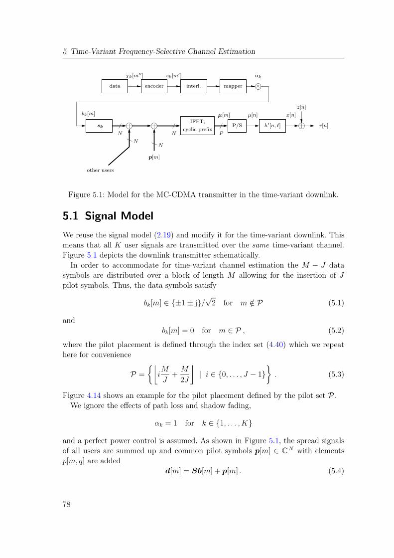
5 Time-Variant Frequency-Selective Channel Estimation
N
IFFT,
cyclic prefixP
p[m]
P/S
µ[n]
h′[n, `]
µ[m] x[n]
r[n]
z[n]
data encoder
ck[m′]
interl. mapper
bk[m]
N
other users
χk[m′′]
N
αk
sk
N
Figure 5.1: Model for the MC-CDMA transmitter in the time-variant downlink.
5.1 Signal Model
We reuse the signal model (2.19) and modify it for the time-variant downlink. This
means that all K user signals are transmitted over the same time-variant channel.
Figure 5.1 depicts the downlink transmitter schematically.
In order to accommodate for time-variant channel estimation the M − J data
symbols are distributed over a block of length M allowing for the insertion of J
pilot symbols. Thus, the data symbols satisfy
bk[m] ∈ {±1 ± j}/√
2 for m /∈ P (5.1)
and
bk[m] = 0 for m ∈ P , (5.2)
where the pilot placement is defined through the index set (4.40) which we repeat
here for convenience
P =
{⌊
iM
J+
M
2J
⌋
| i ∈ {0, . . . , J − 1}}
. (5.3)
Figure 4.14 shows an example for the pilot placement defined by the pilot set P .
We ignore the effects of path loss and shadow fading,
αk = 1 for k ∈ {1, . . . , K}
and a perfect power control is assumed. As shown in Figure 5.1, the spread signals
of all users are summed up and common pilot symbols p[m] ∈ CN with elements
p[m, q] are added
d[m] = Sb[m] + p[m] . (5.4)
78
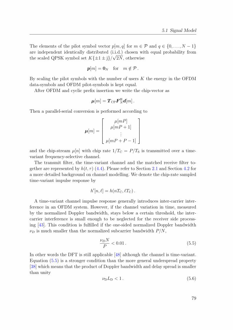
5.1 Signal Model
The elements of the pilot symbol vector p[m, q] for m ∈ P and q ∈ {0, . . . , N − 1}are independent identically distributed (i.i.d.) chosen with equal probability from
the scaled QPSK symbol set K{±1 ± j}/√
2N , otherwise
p[m] = 0N for m /∈ P .
By scaling the pilot symbols with the number of users K the energy in the OFDM
data-symbols and OFDM pilot-symbols is kept equal.
After OFDM and cyclic prefix insertion we write the chip-vector as
µ[m] = T CPF HNd[m] .
Then a parallel-serial conversion is performed according to
µ[m] =
µ[mP ]
µ[mP + 1]...
µ[mP + P − 1]
and the chip-stream µ[n] with chip rate 1/TC = P/TS is transmitted over a time-
variant frequency-selective channel.
The transmit filter, the time-variant channel and the matched receive filter to-
gether are represented by h(t, τ) (4.4). Please refer to Section 2.1 and Section 4.2 for
a more detailed background on channel modelling. We denote the chip-rate sampled
time-variant impulse response by
h′[n, `] = h(nTC, `TC) .
A time-variant channel impulse response generally introduces inter-carrier inter-
ference in an OFDM system. However, if the channel variation in time, measured
by the normalized Doppler bandwidth, stays below a certain threshold, the inter-
carrier interference is small enough to be neglected for the receiver side process-
ing [43]. This condition is fulfilled if the one-sided normalized Doppler bandwidth
νD is much smaller than the normalized subcarrier bandwidth P/N ,
νDN
P< 0.01 . (5.5)
In other words the DFT is still applicable [48] although the channel is time-variant.
Equation (5.5) is a stronger condition than the more general underspread property
[38] which means that the product of Doppler bandwidth and delay spread is smaller
than unity
νDLD < 1 . (5.6)
79

5 Time-Variant Frequency-Selective Channel Estimation
estimatorchannel
FFT
drop prefix,
N
y[m]r[m]
PS/P
r[n]
h[m]
MMSE
demapper
demapper
.
.
.
deinterl.
deinterl.
w′
K [m′]
.
.
.
decoder
decoder
χK [m′′]
χ1[m′′]
.
.
.
w1[m]
wK [m]
w′
1[m′]
Figure 5.2: Model for the MC-CDMA receiver with channel estimation and time-
variant MMSE filter.
We are able to treat the time-variant channel as constant for the duration of each
single OFDM symbol if (5.5) is fulfilled. Hence,
h[m, `] = h′[mP, `] ,
respectively
h[m] =
h[m, 0]...
h[m,L − 1]
∈ C
L×1
in vector notation. The time-variant frequency response g[m] ∈ CN with elements
g[m, q] is defined as the DFT of the time-variant impulse response,
g[m] =√
NF N×Lh[m] .
The receiver removes the cyclic prefix and performs a DFT. The received signal
vector y[m] ∈ CN after these two operations is given by
y[m] = diag (g[m]) (Sb[m] + p[m]) + z[m] , (5.7)
where complex additive white Gaussian noise with zero mean and covariance σ2zIN
is denoted by z[m] ∈ CN with elements z[m, q] for q ∈ {0, . . . , N − 1}.
5.2 Time-Variant Multi-User Detector
Figure 5.2 shows the schematic structure of the downlink receiver. In contrast to the
receiver presented in Section 2.6 for the uplink, we do not use an iterative structure
for the downlink. The main reason for this approach is the fact that, in the downlink,
all users share the same channel. This allows to obtain much better initial channel
80
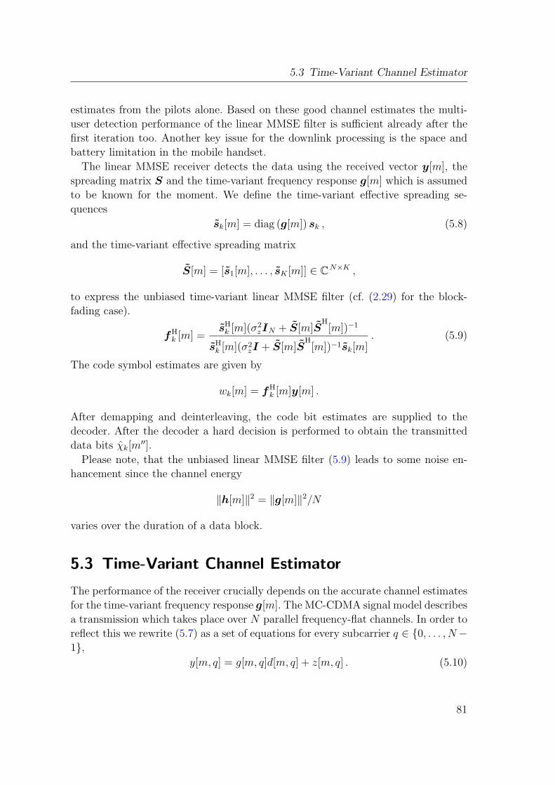
5.3 Time-Variant Channel Estimator
estimates from the pilots alone. Based on these good channel estimates the multi-
user detection performance of the linear MMSE filter is sufficient already after the
first iteration too. Another key issue for the downlink processing is the space and
battery limitation in the mobile handset.
The linear MMSE receiver detects the data using the received vector y[m], the
spreading matrix S and the time-variant frequency response g[m] which is assumed
to be known for the moment. We define the time-variant effective spreading se-
quences
sk[m] = diag (g[m]) sk , (5.8)
and the time-variant effective spreading matrix
S[m] = [s1[m], . . . , sK [m]] ∈ CN×K ,
to express the unbiased time-variant linear MMSE filter (cf. (2.29) for the block-
fading case).
fHk [m] =
sHk [m](σ2
zIN + S[m]SH[m])−1
sHk [m](σ2
zI + S[m]SH[m])−1sk[m]
. (5.9)
The code symbol estimates are given by
wk[m] = fHk [m]y[m] .
After demapping and deinterleaving, the code bit estimates are supplied to the
decoder. After the decoder a hard decision is performed to obtain the transmitted
data bits χk[m′′].
Please note, that the unbiased linear MMSE filter (5.9) leads to some noise en-
hancement since the channel energy
‖h[m]‖2 = ‖g[m]‖2/N
varies over the duration of a data block.
5.3 Time-Variant Channel Estimator
The performance of the receiver crucially depends on the accurate channel estimates
for the time-variant frequency response g[m]. The MC-CDMA signal model describes
a transmission which takes place over N parallel frequency-flat channels. In order to
reflect this we rewrite (5.7) as a set of equations for every subcarrier q ∈ {0, . . . , N −1},
y[m, q] = g[m, q]d[m, q] + z[m, q] . (5.10)
81

5 Time-Variant Frequency-Selective Channel Estimation
where d[m, q] are the elements of d[m] (5.4). Comparing (5.10) with (4.6) we see that
the structure of these equations is identical. The band-limited property of h[m,n]
directly applies to g[m, q] too. This allows to estimate the time-variant frequency-flat
subcarrier g[m, q] with the generalized Slepian basis expansion (4.54). We define
ψi[q] =1
∑
m∈P
|ui[m]p[m, q]|2∑
m∈P
y[m, q]p∗[m, q]u∗i [m] ,
where i ∈ {0, . . . , D − 1} and q ∈ {0, . . . , N − 1}. Although we will use the gener-
alized Slepian basis expansion, we keep the notation regarding the basis expansion
generic. Hence, any basis expansion defined in Chapter 4 can be used for performance
comparison.
The estimated time-variant frequency response is given by
g′[m, q] =D−1∑
i=0
ui[m]ψi[q] .
Further noise suppression is obtained if we exploit the correlation between the sub-
carriers
g[m] = F N×LF HN×Lg′[m] .
Finally, the channel estimates g[m] are inserted into (5.8) and multi-user detection
can be performed.
5.4 Simulation Results
The realizations of the time-variant frequency-selective channel h′[n, `], sampled
at the chip-rate 1/TC, are generated using an exponentially decaying power-delay
profile η2[`] defined in (2.4) and the simulation parameters from Section 3.1.1. These
are: Number of subcarriers N = 64, block length M = 256, essential support of
the channel impulse response L = 15. The discrete time indices n and ` denote
sampling at rate 1/TC = 3.84 ·106 s−1. The exponential decaying power-delay profile
corresponds to a normalized delay spread LD = TD/TC = 1. The autocorrelation for
every channel tap is given by
Rh′h′ [n, `] = η2[`]J0(2πνDPn)
which results in the classical Jakes’ spectrum. We use the enhanced simulation model
(A.1) for every channel tap l ∈ {0, . . . , L − 1}. The simulation uses a chip-rate
sampled time-variant channel, thus any possible effect from residual inter-carrier
interference would be visible in the simulation results.
82
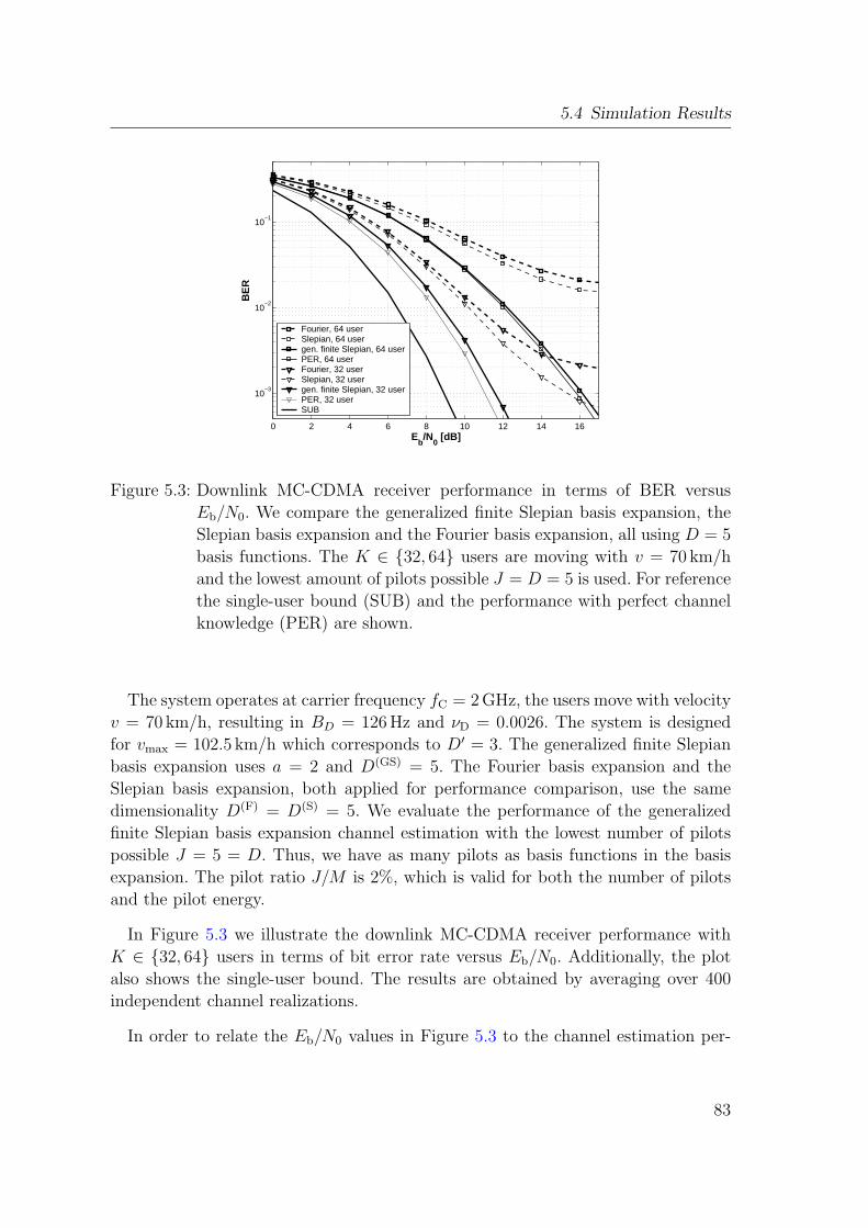
5.4 Simulation Results
0 2 4 6 8 10 12 14 16
10−3
10−2
10−1
Eb/N
0 [dB]
BE
R
Fourier, 64 userSlepian, 64 usergen. finite Slepian, 64 userPER, 64 userFourier, 32 userSlepian, 32 usergen. finite Slepian, 32 userPER, 32 userSUB
Figure 5.3: Downlink MC-CDMA receiver performance in terms of BER versus
Eb/N0. We compare the generalized finite Slepian basis expansion, the
Slepian basis expansion and the Fourier basis expansion, all using D = 5
basis functions. The K ∈ {32, 64} users are moving with v = 70 km/h
and the lowest amount of pilots possible J = D = 5 is used. For reference
the single-user bound (SUB) and the performance with perfect channel
knowledge (PER) are shown.
The system operates at carrier frequency fC = 2 GHz, the users move with velocity
v = 70 km/h, resulting in BD = 126 Hz and νD = 0.0026. The system is designed
for vmax = 102.5 km/h which corresponds to D′ = 3. The generalized finite Slepian
basis expansion uses a = 2 and D(GS) = 5. The Fourier basis expansion and the
Slepian basis expansion, both applied for performance comparison, use the same
dimensionality D(F) = D(S) = 5. We evaluate the performance of the generalized
finite Slepian basis expansion channel estimation with the lowest number of pilots
possible J = 5 = D. Thus, we have as many pilots as basis functions in the basis
expansion. The pilot ratio J/M is 2%, which is valid for both the number of pilots
and the pilot energy.
In Figure 5.3 we illustrate the downlink MC-CDMA receiver performance with
K ∈ {32, 64} users in terms of bit error rate versus Eb/N0. Additionally, the plot
also shows the single-user bound. The results are obtained by averaging over 400
independent channel realizations.
In order to relate the Eb/N0 values in Figure 5.3 to the channel estimation per-
83

5 Time-Variant Frequency-Selective Channel Estimation
formance results in Section 4.3 we establish the relation
ES
N0
=K2
P
M − J
M
Eb
N0
(5.11)
where we took the higher pilot energy in the downlink into account. The simulation
in Figure 5.3 for 0 dB ≤ Eb/N0 ≤ 16 dB and K = 32 users corresponds to ES/N0
values in the range 11 dB ≤ ES/N0 ≤ 27 dB. For K = 64 users the range is from
17 dB ≤ ES/N0 ≤ 33 dB.
Taking (5.11) into account when referring to Figure 4.23 makes clear, that the
drastically smaller MSEM of the generalized finite Slepian basis expansion than of
the Fourier basis expansion leads to a pronounced reduction in bit error rates. This
is because, the Fourier basis expansion is biased as is visible for higher ES/N0 values
in Figure 4.23 which leads to an error floor in Figure 5.3.
Figure 5.3 also shows the receiver performance when using the Slepian basis ex-
pansion. As can be seen in Figure 4.22 and as is explained in Section 4.5 the Slepian
basis expansion performance degrades because of lost orthogonality due to the pi-
lot grid. At the limit J = D the Slepian basis expansion is hardly better than the
Fourier basis expansion. However, this picture changes rapidly with increasing num-
ber of pilots. At J > 10 pilots the performance of the Slepian basis expansion is
practically equivalent to the one of the generalized finite Slepian basis expansion, as
is shown in Figure 4.22.
We also plot the receiver performance for a perfectly known channel (denoted
’PER’) in Figure 5.3, and we can see that the performance advantage of the gen-
eralized finite Slepian basis expansion is strongest at the lowest amount of pilots
possible J = D = 5. The receiver performance is extremely close to the one with
perfect channel knowledge.
5.5 Doppler Diversity in MC-CDMA
In MC-CDMA a data symbol is spread by a user specific spreading code in order to
take advantage of multipath diversity VM. A time-variant channel additionally offers
Doppler diversity VD which can be used in MC-CDMA by convolutional coding and
random interleaving [57]. The intuitive reason for Doppler diversity, respectively
time diversity, is simply the fact that the fading condition of the channel changes
over time. The faster the channel changes the shorter is the duration of a bad channel
realization.
However, accurate time-variant channel state information is required at the re-
ceiver side so that both sources of diversity can be exploited. The overall diversity
of the channel is given by [34]
V = VMVD . (5.12)
84

5.5 Doppler Diversity in MC-CDMA
The Doppler diversity depends on the length of the data block the Doppler spec-
trum and the applied coding scheme. In the next section we derive a measure for
the Doppler diversity that an MC-CDMA receiver is able to take advantage of. This
measure is validated by means of simulation results.
5.5.1 Diversity Measure
In the literature [34] it has been proposed to measure the Doppler diversity VD of a
channel by the product of block length and normalized Doppler bandwidth
VD ≈ M16πνD
9. (5.13)
It is obvious that the shape of the Doppler power spectral density Sgg(ν) may
have an impact on VD as well. For example the Doppler spectrum caused by the
propagation of a single planar wave has the form S1(ν) = δ(ν − νD). Evidently,
such a channel will have a lower Doppler diversity than a rich multipath channel
in an indoor scenario with three dimensional scattering which typically results in a
rectangular Doppler spectrum.
We can interpret a time-variant frequency-flat Rayleigh fading channel g[m] (re-
spectively a subcarrier in an OFDM system) as a stationary Gaussian stochastic
process with corresponding power density spectrum Sgg(ν). Its entropy rate is de-
fined as [36]
h(Sgg) = log 2πe +
∫ 12
− 12
log(Sgg(ν))d ν . (5.14)
However, a typical wireless channel is over-sampled with respect to the Doppler
bandwidth. This is why the support of Sgg(ν) is much smaller than [−1/2, +1/2]
and Sgg(ν) ≡ 0 for νD < |ν| < 1/2 which leads to an ill defined entropy rate
h(Sgg) = −∞ [40] [10, Sec. 4.5]. This fact is the motivation to look for other diversity
measures.
A diversity measure for flat-fading multiple-input multiple-output (MIMO) chan-
nels was defined in [31]. We will show the applicability of the diversity measure
from [31] for time-variant flat-fading single-input single-output channels.
5.5.2 Flat-Fading Multiple-Input Multiple-Output (MIMO)
Channel
A flat-fading MIMO channel is described through a matrix H ∈ CNR×NT where NT
denotes the number of transmit antennas and NR the number of receive antennas.
The elements [H ]r,t describe the fading coefficient between transmit antenna t and
85

5 Time-Variant Frequency-Selective Channel Estimation
receive antenna r. We assume that every element [H ]r,t is complex, circularly sym-
metric, zero mean, and Gaussian distributed which leads to Rayleigh fading. The
covariance matrix of the MIMO channel is defined as
RH = E
{
vec(H) (vec(H))H}
(5.15)
where the operator vec(H) stacks all columns of H . The diversity measure of the
MIMO channel H , given the correlation matrix RH, is defined in [31] as
Ψ(RH) =
(tr(RH)
‖RH‖F
)2
. (5.16)
In the following section we will show how this measure for a flat-fading MIMO
channel can be applied to a time-variant flat-fading single-input single-output chan-
nel.
5.5.3 Time-Variant Flat-Fading Single-Input Single-Output
Channel
In the case of a time-variant frequency-flat subcarrier q we can stack the channel
coefficients g[m, q] in the vector
gq =
g[0, q]...
g[M − 1, q]
∈ C
M ,
for the duration of one data block. We define the covariance matrix of gq as
Rgg = E{gqgHq } ∈ C
M×M
which is independent of subcarrier q if we assume the same Doppler spectrum for
every channel tap.
The elements of g[m, q] fulfill the same statistic properties as the elements of the
MIMO channel matrix [H ]r,t. This is why we are able to insert Rgg into (5.16) in
order to define the diversity measure for a time-variant frequency-flat subcarrier as
Ψ(Rgg) =
(tr(Rgg)
‖Rgg‖F
)2
. (5.17)
We can express (5.17) through the eigenvalues of matrix Rgg. The trace of an
M × M matrix in terms of its eigenvalues is given by
tr(Rgg) =M−1∑
i=0
λi . (5.18)
86
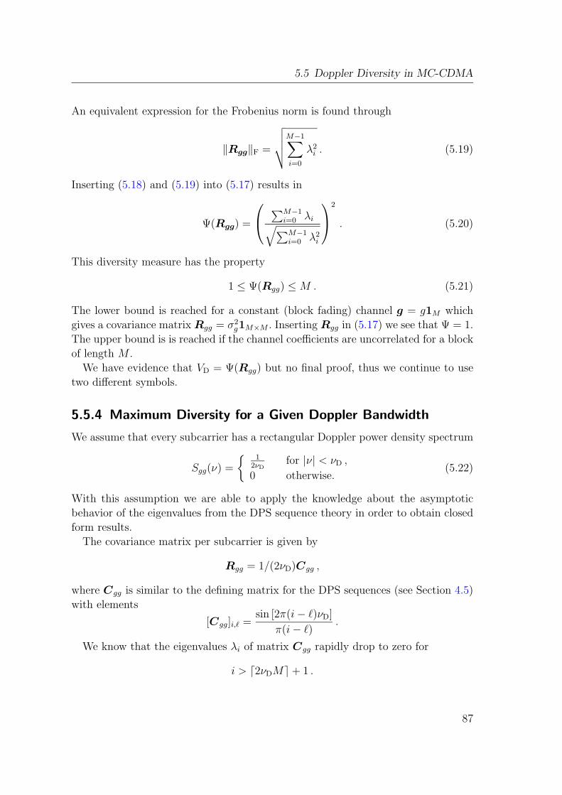
5.5 Doppler Diversity in MC-CDMA
An equivalent expression for the Frobenius norm is found through
‖Rgg‖F =
√√√√
M−1∑
i=0
λ2i . (5.19)
Inserting (5.18) and (5.19) into (5.17) results in
Ψ(Rgg) =
∑M−1i=0 λi
√∑M−1
i=0 λ2i
2
. (5.20)
This diversity measure has the property
1 ≤ Ψ(Rgg) ≤ M . (5.21)
The lower bound is reached for a constant (block fading) channel g = g1M which
gives a covariance matrix Rgg = σ2g1M×M . Inserting Rgg in (5.17) we see that Ψ = 1.
The upper bound is is reached if the channel coefficients are uncorrelated for a block
of length M .
We have evidence that VD = Ψ(Rgg) but no final proof, thus we continue to use
two different symbols.
5.5.4 Maximum Diversity for a Given Doppler Bandwidth
We assume that every subcarrier has a rectangular Doppler power density spectrum
Sgg(ν) =
{1
2νDfor |ν| < νD ,
0 otherwise.(5.22)
With this assumption we are able to apply the knowledge about the asymptotic
behavior of the eigenvalues from the DPS sequence theory in order to obtain closed
form results.
The covariance matrix per subcarrier is given by
Rgg = 1/(2νD)Cgg ,
where Cgg is similar to the defining matrix for the DPS sequences (see Section 4.5)
with elements
[Cgg]i,` =sin [2π(i − `)νD]
π(i − `).
We know that the eigenvalues λi of matrix Cgg rapidly drop to zero for
i > d2νDMe + 1 .
87

5 Time-Variant Frequency-Selective Channel Estimation
Thus, we can give an analytic upper bound for the Doppler diversity measure
Ψ(Rgg) ≤ d2νDMe + 1 . (5.23)
For νDM = c and M → ∞ Equation (5.23) becomes a tight bound, since λi = 1 for
i ≤ d2νDMe and λi = 0 for i > d2νDMe [69] [24, Sec. 5.2]. For arbitrary Doppler
power density spectra with support [−νD, νD] (5.23) is an upper bound.
Definition (5.23) gives a rigorous formulation of the observations made in [47]
where the Fourier basis expansion [60] was used.
5.5.5 Simulation Results
Using the same system parameters as defined in Section 5.4 we simulate a system
with K = 32 users moving with velocity v ∈ {0, 50, 100} km/h which gives BD ∈{0, 93, 185}Hz and νD ∈ {0, 1.9 · 10−3, 3.8 · 10−3}. We use J = 10 OFDM pilot
symbols. The system is designed for vmax = 102.5 km/h which results in a signal
space dimension of D′ = 3. We choose an approximation factor a = 2 and a basis
expansion dimension D(GS) = 5 for the generalized finite Slepian basis expansion.
The results are obtained by averaging over 2000 independent channel realizations.
In Figure 5.4 we illustrate the downlink MC-CDMA receiver performance in terms
of bit error rate versus Eb/N0. With increasing velocity the receiver performs better
because the Doppler diversity VD increases too. For velocities in the range 0 < v <
100km/h the Doppler diversity measure (5.23) is in the range 1 < Ψ < 3 predicting
a similar Doppler diversity VD. In the following we will analyze to which extend our
receiver algorithm is able to take advantage of the predicted Doppler diversity.
The diversity V is defined as the slope of the bit error rate versus Eb/N0 curve
in log-log scale. The power-delay profile defining the multipath diversity VM is kept
constant in this simulation. For velocity v = 0 km/h, the Doppler diversity VD =
1 = Ψ, which follows from the multiplicative assumption in (5.12) and the bound
(5.21). This allows to calculate the additional Doppler diversity that the MC-CDMA
receiver is able to exploit as
VD(v) = V (v)/V (0).
where v denotes the users velocity.
Figure 5.5 plots the Doppler diversity VD versus Eb/N0 for velocity v ∈{50, 100}km/h and a single user K = 1. For the simulations Jakes’ spectrum
was used, for which the diversity measure (5.17) predicts a Doppler diversity of
Ψ(50km/h) = 1.7 and Ψ(100km/h) = 2.8. The obtained Doppler diversity VD as
depicted in Figure 5.5 is clearly much smaller. The reason may be that the selected
transmission and coding scheme does not allow to exploit all diversity. The slight
88

5.5 Doppler Diversity in MC-CDMA
0 2 4 6 8 10 12 14 1610
−4
10−3
10−2
10−1
Eb/N
0 [dB]
BE
R
v=0 km/h, 32 userv=50 km/h, 32 userv=100 km/h, 32 userv=0 km/h, SUBv=50 km/h, SUBv=100 km/h, SUB
Figure 5.4: Downlink MC-CDMA receiver performance in terms of bit-error
rate (BER) versus Eb/N0 for K = 32 users moving with v ∈{0, 50, 100} km/h. For reference the single-user bounds (SUB) are shown
too.
2 3 4 5 6 7 8 9 101
1.1
1.2
1.3
1.4
1.5
1.6
1.7
Eb/N
0 [dB]
VD
v=50 km/h, 1 userv=100 km/h, 1 user
Figure 5.5: Doppler diversity VD exploited by the MC-CDMA system. The diversity
V = VDVM (5.12) is defined as the slope of the bit-error rate versus
Eb/N0 curve in Figure 5.4.
89

5 Time-Variant Frequency-Selective Channel Estimation
decay at higher Eb/N0 values might be due to the bias of the applied time-variant
channel estimation method.
The block-interleaving described in Section 3.3 for block-fading channels results
in a similar diversity increase as the one obtained through Doppler diversity in the
time-variant case.
90

6 Iterative Multi-User Detection and
Time-Variant Channel Estimation
This chapter deals with iterative time-variant channel estimation and multi-user
detection for the uplink of an MC-CDMA system. In iterative receivers the soft in-
formation gained about the transmitted data symbols is used to enhance the channel
estimation and data detection in consecutive iterations. Iterative multi-user detec-
tion and channel estimation for an MC-CDMA uplink was shown in Chapter 3 to
achieve the single-user bound under high load for a block-fading channel. However,
if users are moving at vehicular speed the wireless channel coefficients vary signifi-
cantly over the duration of a single data block. In this chapter we extend the concept
of iterative detection and channel estimation to the time-variant case.
Our results will challenge the reasoning in [5, 72] where a comparison between
different combinations of OFDM and DS-CDMA for cellular communication systems
is given. It is stated that MC-CDMA is best suited for the downlink. For the uplink
MC/DS-CDMA is favored which uses time domain spreading in parallel carriers
with rather large bandwidth per carrier. In [5,72] MC-CDMA is deprecated for the
uplink mainly because the orthogonality of the spreading sequences is destroyed due
to the frequency selective channel. This leads to bad performance for a matched filter
receiver. Furthermore, it is stated that the channel estimation does not perform well
for MC-CDMA.
The results of this chapter will show that MC-CDMA is an excellent choice for
the uplink which allows to exploit both, multipath and Doppler diversity. The basic
prerequisite is iterative multi-user detection. By applying this technique the orthog-
onality of the spreading codes is no necessity any more. Thus, the diversity of the
frequency selective channel can be exploited without drawbacks. However, the en-
hanced performance obtained by multi-user detection does not come at no cost.
The computational complexity is increased since a matrix inversion needs to be per-
formed. Our results are applicable to an isolated-cell scenario since no scrambling
code is applied.
Accurate channel estimates are mandatory for iterative multi-user detection algo-
rithms. In the following sections we use the iterative multi-user receiver structure to
91

6 Iterative Multi-User Detection and Time-Variant Channel Estimation
data encoder interl. mapper
N N
IFFT,
cyclic prefixP
pk[m]
sk P/S
µk[n]µk[m] xk[n]
N
bk[m]
r[n]
z[n]
χk[m′′] ck[m′]
other users
αk
h′
k[n, `]
Figure 6.1: Model for the MC-CDMA transmitter and the channel in the uplink.
design a new iterative time-variant channel estimation scheme. This iterative time-
variant channel estimation scheme uses the feedback soft symbols, that are derived
from the output of the soft-in soft-out decoder, in order to enhance the channel es-
timates. The channel estimation itself is performed individually for every subcarrier
but jointly for all users. The time-variant subcarrier is modelled by the Slepian basis
expansion from Section 4.5. By using the Slepian basis expansion the dimensional-
ity of the time-variant estimation problem can be drastically reduced and we do not
need the detailed knowledge of second order statistics.
6.1 Uplink Signal Model for Time-Variant
Frequency-Selective Channels
We extend the downlink signal model (5.7) to the uplink case where every user trans-
mits over a different channel and uses a unique (random) pilot sequence. Figure 6.1
shows the schematic transmitter and channel model for the uplink. The M −J data
symbols are distributed over a block of length M fulfilling
bk[m] ∈ {±1 ± j}/√
2 for m /∈ P (6.1)
and
bk[m] = 0 for m ∈ P (6.2)
allowing for pilot symbol insertion. The pilot placement is defined through the pilot
set P (4.40), see also Figure 4.14.
After spreading, pilot symbols pk[m] ∈ CN with elements pk[m, q] are added
dk[m] = skbk[m] + pk[m] . (6.3)
92

6.2 Iterative Time-Variant Multi-User Detection
The elements of the pilot symbols pk[m, q] for m ∈ P and q ∈ {0, . . . , N−1} are i.i.d.
chosen with equal probability from the QPSK symbol set {±1 ± j}√
2N , otherwise
pk[m] = 0N for m /∈ P .
Then, an N point inverse DFT is performed and a cyclic prefix of length G is
inserted. Each single OFDM symbol together with the cyclic prefix is represented
by µk[m] ∈ CP and has length P = N + G chips. We write
µk[m] = T CPF HNdk[m] .
After parallel-serial conversion according to
µk[m] =
µk[mP ]
µk[mP + 1]...
µk[mP + P − 1]
the chip stream µk[n] with chip rate 1/TC = P/TS is transmitted over a time-
variant frequency-selective channel hk[m]. We assume the same channel conditions
as defined in Section 5.1 with (5.5), so that the inter-carrier interference is negligibly
small.
At the receive antenna all K user signals add up. The receiver removes the cyclic
prefix and performs a DFT. The received signal vector after these two operations is
given by
y[m] =K∑
k=1
diag (gk[m]) (skbk[m] + pk[m]) + z[m] , (6.4)
where complex additive white Gaussian noise with zero mean and covariance σ2zIN
is denoted by z[m] ∈ CN with elements z[m, q].
6.2 Iterative Time-Variant Multi-User Detection
We define the time-variant effective spreading sequences
sk[m] = diag (gk[m]) sk , (6.5)
and the time-variant effective spreading matrix
S[m] = [s1[m], . . . , sK [m]] ∈ CN×K .
Using these definitions we write a signal model for data detection
y[m] = Sk[m]b[m] + z[m] for m /∈ P
93
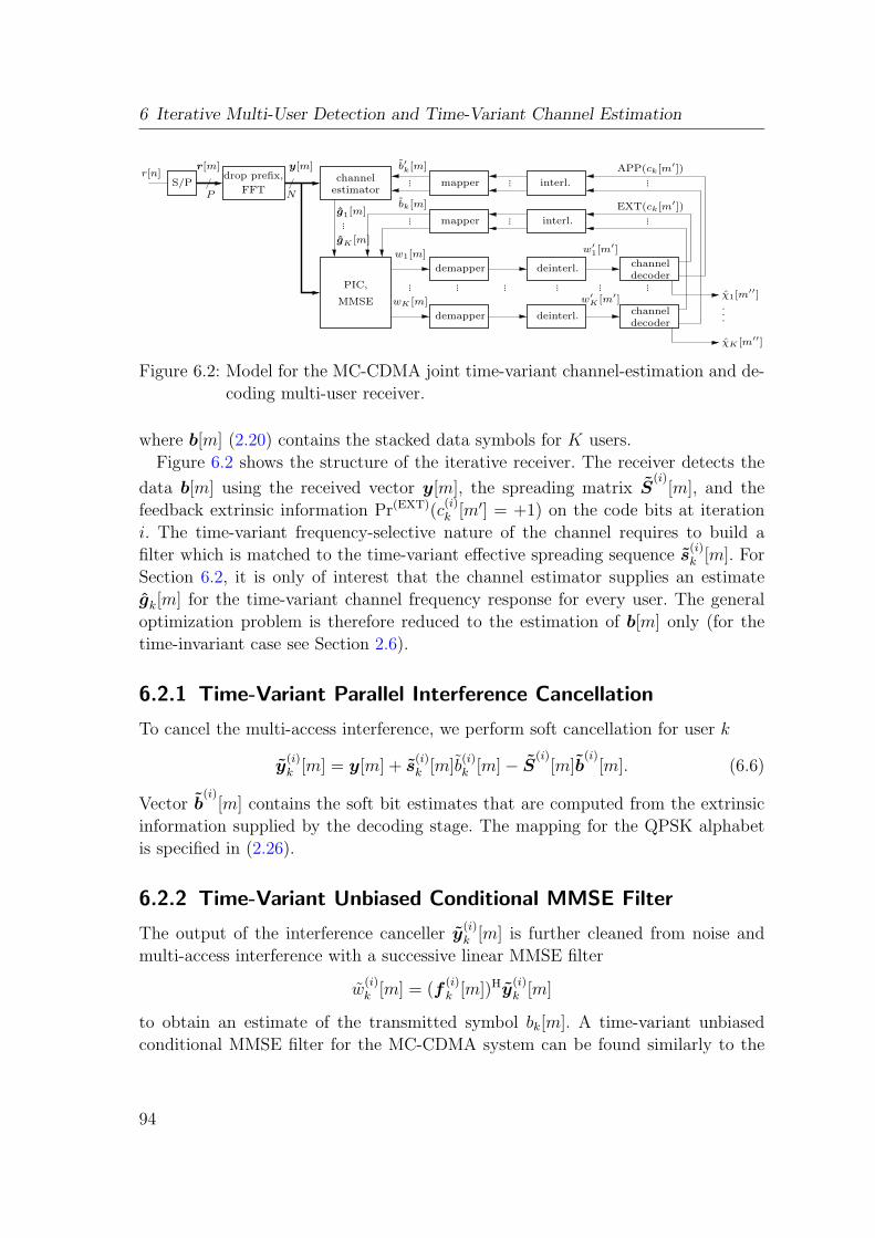
6 Iterative Multi-User Detection and Time-Variant Channel Estimation
... ...
......
......... ... ... ... ... ...
...
deinterl.
deinterl.
interl.
interl.
channeldecoder
channeldecoder
mapper
mapper
demapper
demapper
PIC,
MMSE
estimatorchanneldrop prefix,
FFTS/P
r[n]
P N
r[m] y[m]
.
.
.
χK [m′′]
APP(ck[m′])
EXT(ck[m′])
w′
1[m′]
χ1[m′′]
g1[m]
gK
[m]
w1[m]
wK [m]
b′k[m]
bk[m]
w′
K[m′]
Figure 6.2: Model for the MC-CDMA joint time-variant channel-estimation and de-
coding multi-user receiver.
where b[m] (2.20) contains the stacked data symbols for K users.
Figure 6.2 shows the structure of the iterative receiver. The receiver detects the
data b[m] using the received vector y[m], the spreading matrix S(i)
[m], and the
feedback extrinsic information Pr(EXT)(c(i)k [m′] = +1) on the code bits at iteration
i. The time-variant frequency-selective nature of the channel requires to build a
filter which is matched to the time-variant effective spreading sequence s(i)k [m]. For
Section 6.2, it is only of interest that the channel estimator supplies an estimate
gk[m] for the time-variant channel frequency response for every user. The general
optimization problem is therefore reduced to the estimation of b[m] only (for the
time-invariant case see Section 2.6).
6.2.1 Time-Variant Parallel Interference Cancellation
To cancel the multi-access interference, we perform soft cancellation for user k
y(i)k [m] = y[m] + s
(i)k [m]b
(i)k [m] − S
(i)[m]b
(i)[m]. (6.6)
Vector b(i)
[m] contains the soft bit estimates that are computed from the extrinsic
information supplied by the decoding stage. The mapping for the QPSK alphabet
is specified in (2.26).
6.2.2 Time-Variant Unbiased Conditional MMSE Filter
The output of the interference canceller y(i)k [m] is further cleaned from noise and
multi-access interference with a successive linear MMSE filter
w(i)k [m] = (f
(i)k [m])Hy
(i)k [m]
to obtain an estimate of the transmitted symbol bk[m]. A time-variant unbiased
conditional MMSE filter for the MC-CDMA system can be found similarly to the
94

6.3 Iterative Time-Variant Channel Estimation
MMSE detector given in Section 2.6. In order to simplify the notation we omit the
iteration index i for the filter. It has the form
fHk [m] =
sHk [m](σ2
zIN + S[m]V [m]SH[m])−1
sHk [m](σ2
zI + S[m]V [m]SH[m])−1sk[m]
,
cf. (2.29) for the block-fading case.
Matrix V [m] denotes the error covariance matrix
V [m] = Eb
{
(b[m] − b[m])(b[m] − b[m])H}
(6.7)
with diagonal elements
[V [m]]k,k = 1 − |b(i)k [m]|2 , (6.8)
the non-diagonal elements are assumed to be zero. In this case we calculate the
variance for the symbol at time instant m belonging to user k and consider the filter
conditional.
6.3 Iterative Time-Variant Channel Estimation
The performance of the iterative receiver crucially depends on the accurate channel
estimates for the time-variant frequency response gk[m]. The MC-CDMA signal
model (6.4) shows that the transmission takes place over N parallel frequency-flat
channels. We rewrite (6.4) as a set of equations for every subcarrier q ∈ {0, . . . , N −1},
y[m, q] =K∑
k=1
gk[m, q](sk[q]bk[m] + pk[m, q]) + z[m, q] . (6.9)
Comparing (6.9) with (5.10) makes clear why the channel estimation in the up-
link is substantially more complicated than in the downlink. For every subcarrier
q we need to estimate the additive mixture of K bandlimited processes gk[m, q].
We describe the band limited property of each users’ process by the Slepian basis
expansion from Section 4.5. A linear MMSE filter is applied to estimate the basis
expansion coefficients using pilots and soft symbols in an iterative process.
6.3.1 Signal Model for Time-Variant Channel Estimation
For the downlink, as described in Section 5, we used the generalized finite Slepian
basis expansion without iterative processing to perform channel estimation. In the
downlink all users share the same channel, thus the effective ES/N0 for the channel
estimation is high enough in order to obtain time-variant channel estimates with
95

6 Iterative Multi-User Detection and Time-Variant Channel Estimation
good accuracy, see Section 5.4. The generalized finite Slepian basis expansion per-
forms channel estimation using the pilot pattern P and interpolation between the
pilot positions.
In the uplink the ES/N0 is drastically reduced since channels for K individual
users have to be estimated. In the uplink the available processing power is much
higher such we can afford iterative processing. During the iterative process channel
knowledge for the full data block may be obtained, thus the orthogonality of the
Slepian basis functions can be maintained. The higher amount of pilots necessary for
the uplink due to the small ES/N0 reduces the performance gain of the generalized
finite Slepian basis expansion (see Section 4.8.5). This is why we use the Slepian
basis expansion also for the first iteration where only pilots are used for the initial
channel estimate.
Substituting the Slepian basis expansion (4.28) for the time-variant subcarrier
coefficients gk[m, q] into the system model (6.9) we obtain
y[m, q] =K∑
k=1
D−1∑
i=0
ui[m]ψk[i, q]dk[m, q] + z[m, q] , (6.10)
where
dk[m, q] = sk[q]bk[m] + pk[m, q] . (6.11)
An estimate of the subcarrier coefficients ψk[i, q] can be obtained jointly for all K
users but individually for every subcarrier q. We define the vector
ψq =
ψ1[0, q]...
ψK [0, q]...
ψ1[D − 1, q]...
ψK [D − 1, q]
∈ CKD
containing the basis expansion coefficients of all K users for subcarrier q. Further-
more, we introduce
yq =
y[0, q]...
y[M − 1, q]
∈ C
M
for the received symbol sequence on subcarrier q for each single data block. Using
these definitions we write
yq = Dqψq + zq , (6.12)
96

6.3 Iterative Time-Variant Channel Estimation
where
Dq = [diag (u0) Dq, . . . , diag (uD−1) Dq] ∈ CM×KD , (6.13)
and Dq ∈ CM×K (3.3) contains the transmitted symbols for all K users on subcarrier
q which we repeat here for convenience
Dq =
d1[0, q] . . . dK [0, q]...
. . ....
d1[M − 1, q] . . . dK [M − 1, q]
.
For channel estimation, J pilot symbols in (6.11) are known. The remaining M − J
data symbols are not known. We replace them by soft symbols, calculated from the
a-posteriori probability (3.5) obtained in the previous iteration. This enables us to
obtain refined channel estimates if the soft symbols get more certain from iteration
to iteration. For the first iteration the soft symbols b′k[m] for m /∈ P are set to zero.
We define the soft symbol matrix Dq ∈ CM×K according to (3.3) by replacing
dk[m, q] with
dk[m, q] = sk[q]b′k[m] + pk[m, q] .
The soft symbols b′k[m] are defined according to (3.5). Finally we define Dq ∈C
M×KD according to (6.13) by replacing Dq with Dq. The matrix Dq contains
deterministic pilot symbols and statistical information about the transmitted data
symbols.
6.3.2 Linear MMSE Channel Estimation
We extend the results obtained in Section 3.2 to the time-variant case. The linear
MMSE estimate of ψq in (6.12) is given by (with the subcarrier index q omitted)
ψLMMSE = DH
DD
H+ Λ
′ + σ2zIM
︸ ︷︷ ︸
,∆′
−1
y. (6.14)
where the elements of the diagonal matrix Λ′ are defined as
[Λ′]m,m =K∑
k=1
D−1∑
i=0
1
Nu2
i [m]var{bk[m]}, (6.15)
and the symbol variance is
var{bk[m]} = Eb
{(
bk[m] − Eb{bk[m]}
)2}
= 1 − b2k[m].
97

6 Iterative Multi-User Detection and Time-Variant Channel Estimation
The elements of the basis function are denoted by ui[m] (see Section 4.5).
For evaluation of this estimator it is necessary to invert an M -dimensional matrix,
which is computationally expensive. To avoid this, we apply the matrix inversion
lemma to (6.14), yielding
ψLMMSE =(
DH∆
′−1D + IK
)−1
DH∆
′−1y. (6.16)
The rows of matrix D are scaled by the diagonal matrix ∆′, taking into account the
variances of the noise and the variance of the soft symbol estimates.
After estimating ψq for all q ∈ {0, . . . , N − 1} an estimate for the time-variant
frequency response is given by
g′k[m, q] =
D−1∑
i=0
ui[m]ψk[i, q] .
Further noise suppression is obtained if we exploit the correlation between the sub-
carriers
gk[m] = F N×LF HN×Lg′
k[m] .
Finally, this allows to perform data detection by inserting the channel estimates
gk[m] into (6.5). Figure 6.3 shows a summary of the iterative channel estimation
algorithm.
Input:
y ∈ CN , b′k[m] ∈ C, σ2
z ∈ R.
Uses:
pk[m, q] ∈ C, sk[q] ∈ C, ui[m] ∈ R for i ∈ {0, . . . ,D − 1}.Index ranges:
k ∈ {1, . . . ,K}, m ∈ {0, . . . ,M − 1}, q ∈ {0, . . . , N − 1}.Channel estimation:
[Λ′]m,m =∑K
k=1
∑D−1i=0
1N
u2i [m](1 − b2
k[m]),
∆′ = Λ
′ − σ2zIM ,
[Dq]m,k = sk[q]b′k[m] + pk[m, q],
ψq,LMMSE =(
DH
q∆′−1
Dq + IK
)−1
DH
q ∆′−1
y,
g′k[m, q] =∑D−1
i=0 ui[m]ψk[i, q],
gk[m] = F N×LF HN×Lg′
k[m].
Output:
gk[m] ∈ CN .
Figure 6.3: Iterative channel estimation algorithm. Each line is evaluated for the
defined index ranges if a certain index appears on the left hand side.
98

6.3 Iterative Time-Variant Channel Estimation
0 2 4 6 8 10 12 1410
−4
10−3
10−2
10−1
Eb/N
0 [dB]
BE
R
K=64, v=0K=64, v=100K=32, v=0K=32, v=100basis expansion SUB, v=0SUB, v=0
Figure 6.4: MC-CDMA uplink performance in terms of bit error rate (BER) ver-
sus Eb/N0 after 4 iterations. The Slepian basis expansion uses D′ =
D = 3 basis functions. The K ∈ {32, 64} users are moving with
v ∈ {0, 100} km/h. The normalized delay spread LD = 4. For refer-
ence, the single-user bound (SUB) and the basis expansion single-user
bound both for v = 0 km/h are shown too.
6.3.3 Simulation Results
The realizations of the time-variant frequency-selective channel h′k[n, `], sampled at
the chip-rate 1/TC, are generated using the parameters from Section 5.4.
The system operates at carrier frequency fC = 2 GHz and the K ∈ {32, 64}users move with velocity v ∈ {0, 100} km/h. This gives a Doppler frequency BD ∈{0, 190}Hz and νD ∈ {0, 3.8 · 10−3}. The number of subcarriers N = 64 and the
OFDM symbol with cyclic prefix has length of P = G + N = 79. The data block
consists of M = 256 OFDM symbols with J = 60 OFDM pilot symbols. The system
is designed for vmax = 102.5 km/h which results in D = D′ = 3 for the Slepian basis
expansion. The simulation results are obtained by averaging over 100 independent
channel realizations.
Figure 6.4 illustrates the MC-CDMA uplink performance with iterative time-
variant channel estimation based on the Slepian basis expansion in term of bit error
rate versus Eb/N0 after four iterations. The plot also shows the single-user bound
which is defined as the performance for one user K = 1 and a perfectly known
channel gk[m]. Additionally, we plot the basis expansion single-user bound. This is
the performance which can be achieved with the Slepian basis expansion channel-
99
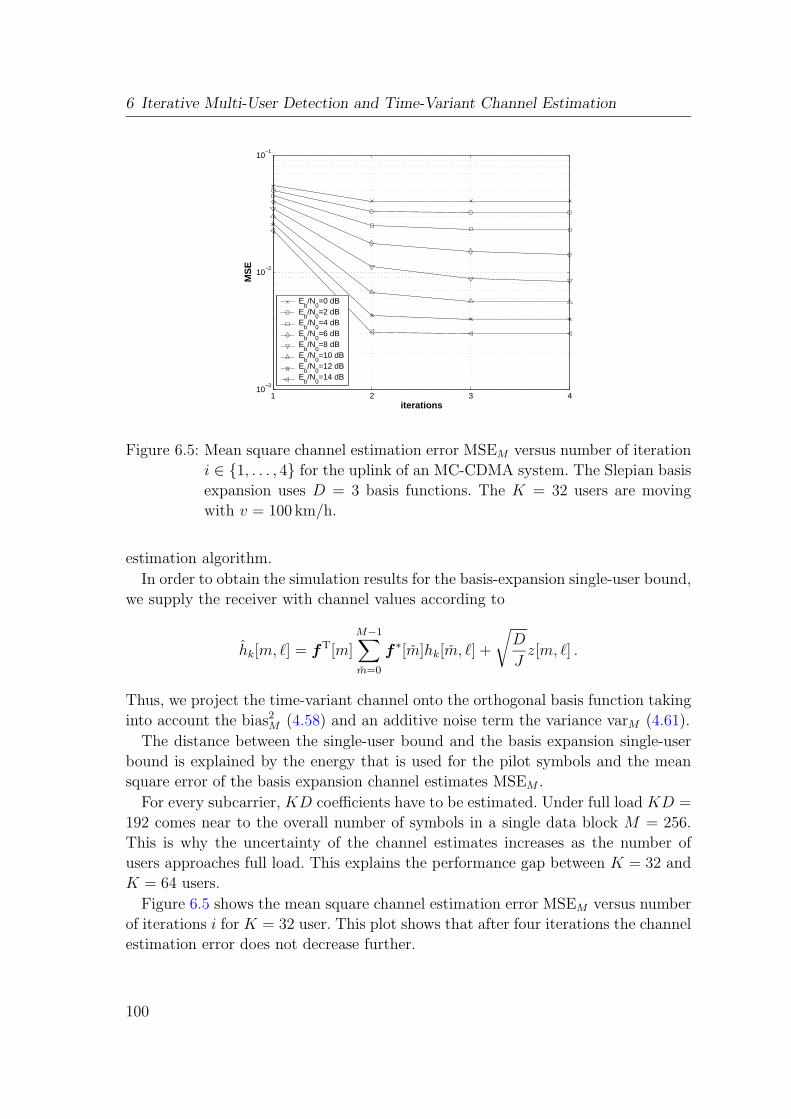
6 Iterative Multi-User Detection and Time-Variant Channel Estimation
1 2 3 410
−3
10−2
10−1
iterations
MS
E
Eb/N
0=0 dB
Eb/N
0=2 dB
Eb/N
0=4 dB
Eb/N
0=6 dB
Eb/N
0=8 dB
Eb/N
0=10 dB
Eb/N
0=12 dB
Eb/N
0=14 dB
Figure 6.5: Mean square channel estimation error MSEM versus number of iteration
i ∈ {1, . . . , 4} for the uplink of an MC-CDMA system. The Slepian basis
expansion uses D = 3 basis functions. The K = 32 users are moving
with v = 100 km/h.
estimation algorithm.
In order to obtain the simulation results for the basis-expansion single-user bound,
we supply the receiver with channel values according to
hk[m, `] = fT[m]M−1∑
m=0
f ∗[m]hk[m, `] +
√
D
Jz[m, `] .
Thus, we project the time-variant channel onto the orthogonal basis function taking
into account the bias2M (4.58) and an additive noise term the variance varM (4.61).
The distance between the single-user bound and the basis expansion single-user
bound is explained by the energy that is used for the pilot symbols and the mean
square error of the basis expansion channel estimates MSEM .
For every subcarrier, KD coefficients have to be estimated. Under full load KD =
192 comes near to the overall number of symbols in a single data block M = 256.
This is why the uncertainty of the channel estimates increases as the number of
users approaches full load. This explains the performance gap between K = 32 and
K = 64 users.
Figure 6.5 shows the mean square channel estimation error MSEM versus number
of iterations i for K = 32 user. This plot shows that after four iterations the channel
estimation error does not decrease further.
100

6.3 Iterative Time-Variant Channel Estimation
1 2 3 410
−3
10−2
10−1
iterations
MS
E
Eb/N
0=0 dB
Eb/N
0=2 dB
Eb/N
0=4 dB
Eb/N
0=6 dB
Eb/N
0=8 dB
Eb/N
0=10 dB
Eb/N
0=12 dB
Eb/N
0=14 dB
Figure 6.6: Means square channel estimation error MSEM versus number of iteration
i ∈ {1, . . . , 4} for the uplink of an MC-CDMA system. The Slepian basis
expansion uses D = 3 basis functions. The K = 64 users are moving
with v = 100 km/h.
The picture is different for K = 64 users as is shown in Figure 6.6. Here it can be
seen that it would be beneficial to perform more iterations at higher Eb/N0 values.
101

6 Iterative Multi-User Detection and Time-Variant Channel Estimation
102

7 Conclusions
This thesis deals with OFDM multi-user communication over time-variant chan-
nels. We investigated MC-CDMA that combines OFDM with frequency domain
spreading. We applied iterative multi-user detection based on parallel interference
cancellation and MMSE filtering.
Instrumental for any multi-user detection algorithm are accurate channel esti-
mates. We developed new iterative channel estimation methods that combine pilots
with feedback soft-symbols to enhance the quality of the channel estimates. Further-
more, statistical information about the soft-symbols, like the mean and the variance,
are exploited using a channel estimator based on the MMSE criterion.
The thesis can be divided into two parts. The first part in Chapter 2 and 3 deals
with block fading channels where the channel is assumed to stay constant for the
duration of a data block. The second part in Chapter 4, 5 and 6 deals with time-
variant channels which vary significantly over the duration of data block.
Block Fading Channels
In the following we list key findings and conclusions specific to block fading channels:
• We showed that an MC-CDMA system, while having the same complexity
for data-detection as DS-CDMA, has a drastically reduced channel estimation
complexity especially at high bit rates. This is due to the fact that the channel
estimation complexity for MC-CDMA grows linearly with the essential sup-
port of the channel impulse response L. While in DS-CDMA, because of time
domain processing, the complexity increases with L3.
• The performance increase through block interleaving is not linear in the num-
ber of blocks. This is linked to the constrained length of the applied code.
Time-Variant Channels
In the following we will present key findings and conclusions for time-variant chan-
nels:
103

7 Conclusions
• OFDM transmission over time-variant channels is susceptible to inter-carrier
interference. But, the delay spread of mobile-communication channels is still
short enough so that the subcarrier bandwidth can be chosen much larger than
the Doppler bandwidth while retaining acceptable spectral efficiency. Such a
design results in time-variant frequency-flat subcarriers that are independent
of each other.
• We investigated time-variant channel estimation methods that do not need
knowledge of detailed second order statistics. We assumed an upper bound
for the maximum Doppler bandwidth only. The classical Fourier basis expan-
sion was analyzed and its weaknesses which stems from windowing and the
associated spectral leakage were discussed.
• We introduced the concepts from the theory of time-concentrated and band-
limited sequences to the field of channel estimation and modelling by designing
a Slepian basis expansion. The Slepian basis expansion is characterized by two
parameters only: the maximum velocity of the users and the block length. For
practical communication systems at 2 GHz with users at vehicular velocities up
to 100 km/h the Slepian basis expansion needs as few as three basis functions
in order to describe the time-variant channel. The basis expansion is suitable
for a whole ensemble of channel realization as long as the velocity of the user
is below the chosen upper bound.
• Analytic performance results for time-variant frequency-flat channels, respec-
tively subcarriers, were established. We could show that the square bias of the
Slepian basis expansion is more than a magnitude smaller than the square bias
of the Fourier basis expansion.
• We derived a novel generalized finite Slepian basis expansion and applied it
to pilot-based time-variant channel estimation on a per-subcarrier basis for an
MC-CDMA downlink. With the generalized finite Slepian basis expansion we
are able to perform low complexity time-variant channel estimation for each
single data block using evenly distributed pilots. Additionally, interpolation
between the pilot positions is performed by the basis expansion too.
• We extended the iterative MC-CDMA receiver for the uplink to the time-
variant case using the Slepian basis expansion, achieving a consistent perfor-
mance for a wide range of velocities.
• It is important to emphasize that the situation in a mobile communication
system is different to the one in a single-frequency broadcasting network that
uses DVB-T or DAB. Such broadcasting systems have a more pronounced
104
inter-carrier interference problem since the overall design has to accommodate
for the large distances between individual transmitters that all use the same
carrier frequency.
• We derived a simulation model with correct Rayleigh fading statistics over the
full velocity range. We found that the receiver performance strongly depends
on the statistical fading property of the channel.
• The results presented in this thesis for the uplink scenario can be easily extend
to a MIMO multi-user system where every user has one transmit antenna and
the base station has NR receive antennas. First work on this issue can be found
in [49]. Further analysis using a geometry based stochastic channel model was
performed in [28].
• We showed that Doppler diversity can be exploited by an MC-CDMA system if
accurate time-variant channel estimation based on the Slepian basis expansion
is used. Thus the receiver performs better at higher speed.
• In [5,72] it is stated that MC-CDMA has several drawbacks which hinders its
application in the uplink. This drawbacks are namely the destroyed orthogo-
nality of the spreading codes due to the frequency selective channels and the
not adequate channel estimation quality. However, the analysis in [5, 72] was
conducted for an receiver based on a single user matched filter. We showed in
this thesis that by applying iterative multi-user detection and iterative time-
variant channel estimation MC-CDMA becomes a very interesting candidate
for future 4G systems. We showed that MC-CDMA can achieve excellent per-
formance for time-variant channels in the uplink.
105

7 Conclusions
106

A Simulation Model for
Time-Variant Channels with
Jakes’ Spectrum
We use the model from [93] and correct it so that the Rayleigh distribution of h[m]
is maintained at low velocities and at v = 0 km/h. The detailed simulation model
for h[m] is defined as follows:
h[m] =1√2(hc[m] + jhs[m]) (A.1)
hc[m] =2√A
A∑
i=1
cos(ψi) · cos(2πνDm cos αi + φi) (A.2)
hs[m] =2√A
A∑
i=1
sin(ψi) · cos(2πνDm cos αi + φi)
with
αi =2πi − π + φ
4Afor i ∈ {1, . . . , A}
where φ, φi, and ψi are independent and uniformly distributed over [−π, π) for all
i. For the numerical simulations we fix the number of interfering paths to A = 20.
In the limit νD = 0 equation (A.2) reduces to
hc[m] =2√A
A∑
i=1
cos(ψi) · cos(φi) . (A.3)
Because of the central limit theorem and the independence of all ψi and φi the
channel coefficients hc[m] are normally distributed. Therefore, the model converges
to a block fading channel.
In [93] φi is replaced by a common phase φ. In this case the components of the
sum in (A.3) are not independent and the channel coefficients hc[m] are not normally
distributed.
107

A Simulation Model for Time-Variant Channels with Jakes’ Spectrum
108
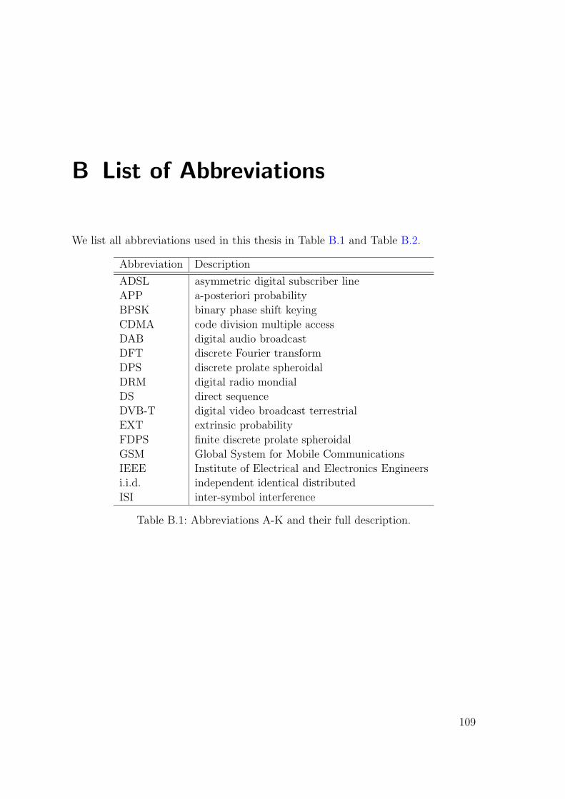
B List of Abbreviations
We list all abbreviations used in this thesis in Table B.1 and Table B.2.
Abbreviation Description
ADSL asymmetric digital subscriber line
APP a-posteriori probability
BPSK binary phase shift keying
CDMA code division multiple access
DAB digital audio broadcast
DFT discrete Fourier transform
DPS discrete prolate spheroidal
DRM digital radio mondial
DS direct sequence
DVB-T digital video broadcast terrestrial
EXT extrinsic probability
FDPS finite discrete prolate spheroidal
GSM Global System for Mobile Communications
IEEE Institute of Electrical and Electronics Engineers
i.i.d. independent identical distributed
ISI inter-symbol interference
Table B.1: Abbreviations A-K and their full description.
109
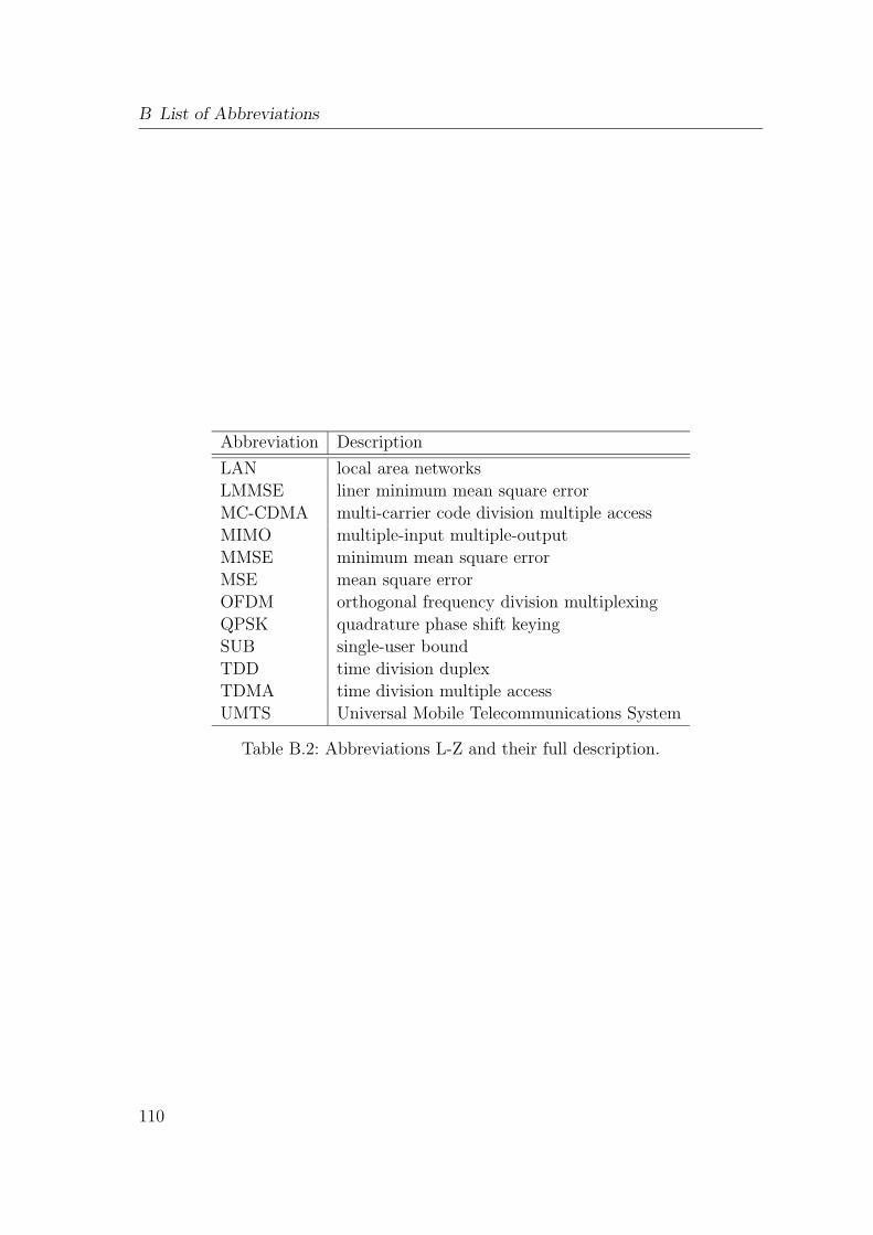
B List of Abbreviations
Abbreviation Description
LAN local area networks
LMMSE liner minimum mean square error
MC-CDMA multi-carrier code division multiple access
MIMO multiple-input multiple-output
MMSE minimum mean square error
MSE mean square error
OFDM orthogonal frequency division multiplexing
QPSK quadrature phase shift keying
SUB single-user bound
TDD time division duplex
TDMA time division multiple access
UMTS Universal Mobile Telecommunications System
Table B.2: Abbreviations L-Z and their full description.
110

C List of Symbols
We list here symbols that are generally used throughout the thesis. Locally used
symbols are omitted. We list Greek symbols in Table C.1, lower case symbols in
Table C.2, and upper case symbols in Table C.3.
Symbol Description
α user power
β load in a communication system
γ time domain basis expansion coefficient
η2 power delay profile
λ eigenvalue
µ transmitted chip
ν normalized frequency
νD normalized Doppler bandwidth (frequency)
ξ sufficient statistic
σ2, σ variance, singular value
ψ frequency domain basis expansion coefficient
Ψ diversity measure
χ information bit
Table C.1: Greek symbols.
111

C List of Symbols
Symbol Description
a approximation factor for finite Slepian basis expansion
b data symbol
b soft symbol
c code bit
c0 speed of light
d transmitted symbol
fC carrier frequency
g channel frequency response
h channel impulse response
i, ` general index
j√−1
k user index
m discrete time at symbol rate 1/TS
n discrete time at chip rate 1/TC
p pilot symbol
q subcarrier index
r received chip with noise
s spreading sequence
s effective spreading sequence
u basis function
v velocity
w channel value after detector
x received chip without noise
y received symbol after cyclic prefix removal and DFT
z noise
Table C.2: Lower case symbols.
112

Symbol Description
A number of interfering paths per channel tap
B number of data blocks used for interleaving
BD one sided Doppler bandwidth
D dimension of the basis expansion
Eb energy per information bit
ES energy per data symbol
G length of cyclic prefix
J number of pilot symbols per data block
K number of users
L essential support of the channel impulse response
LD root mean square delay spread normalized to the sampling rate
TD root mean square delay spread
M number of symbols per data block
N number of subcarriers, length of spreading sequence
N0 noise power spectral density
NR number of receive antennas
NT number of transmit antennas
P length of an OFDM symbol including the cyclic prefix
P set of pilot positions
R autocorrelation
R covariance matrix
RC code rate of the convolutional encoder
RS code rate of the symbol mapper
S power spectral density
S spreading matrix
S effective spreading matrix
TC chip duration
TD root mean square delay spread
TS symbol duration
V diversity
VD Doppler diversity
VM multipath diversity
X set of data sybols
Table C.3: Upper case symbols.
113

C List of Symbols
114

Bibliography
[1] 3GPP, “Third Generation Partnership Project (3GPP).” [Online]. Available:
http://www.3gpp.org/ 1
[2] ——, “Feasibility study for OFDM for UTRAN enhancement,” 3GPP TR
25.892 V1.1.0, March 2004. [Online]. Available: http://www.3gpp.org/ 2
[3] C. H. Aldana, E. de Carvalho, and J. M. Cioffi, “Channel estimation for mul-
ticarrier multiple input single output systems using the EM algorithm,” IEEE
Transactions on Signal Processing, vol. 51, no. 12, pp. 3280–3292, December
2003. 33
[4] H. Artes, F. Hlawatsch, and G. Matz, “Efficient POCS algorithms for determin-
istic blind equalization of time-varying channels,” in IEEE Global Telecommuni-
cation Conference (GLOBECOM), vol. 2, San Francisco (CA), USA, November
2000, pp. 1031–1035. 49
[5] H. Atarashi, S. Abeta, and M. Sawahashi, “Broadband packet wireless access
appropriate for high-speed and high-capacity throughput,” in IEEE Vehicular
Technology Conference (VTC), vol. 1, May 2001, pp. 566–570. 91, 105
[6] L. R. Bahl, J. Cocke, F. Jelinek, and J. Raviv, “Optimal decoding of linear
codes for minimizing symbol error rate,” IEEE Transactions on Information
Theory, vol. 20, no. 2, pp. 284–287, Mar. 1974. 2, 21, 24
[7] S. Barbarossa and A. Scaglione, Signal Processing Advances in Wireless and
Mobile Communications. Upper Saddle River (NJ), USA: Prentice-Hall, Inc.,
2000, vol. 2, ch. Time-Varying Fading Channels. 41
[8] I. Barhumi, G. Leus, and M. Moonen, “Time-varying FIR equalization of
doubly-selective channels,” in IEEE International Conference on Communi-
cations (ICC), vol. 5, Anchorage (AK), USA, May 2003, pp. 3246–3250. 49
[9] P. Bello, “Characterization of randomly time-variant linear channels,” IEEE
Trans. Comm. Syst., vol. CS-11, no. 4, pp. 360–393, December 1963. 3, 42
115
Bibliography
[10] T. Berger, Rate Distortion Theory, T. Kailath, Ed. Englewood Cliffs (NJ),
USA: Prentice-Hall, Inc., 1971. 85
[11] J. A. C. Bingham, “Multicarrier modulation for data transmission: An idea
whose time has come,” IEEE Transactions on Communications, vol. 28, no. 5,
pp. 5–14, 1990. 2, 10
[12] T. P. Bronez, “Spectral estimation of irregularly sampled multideminsional
processes by generalized prolate spheroidal sequences,” IEEE Transactions on
Acoustics, Speech, and Signal Processing, vol. 36, no. 12, pp. 1862–1873, De-
cember 1988. 60
[13] G. Caire and U. Mitra, “Structured multiuser channel estimation for block-
synchronous DS/CDMA,” IEEE Transactions on Communications, vol. 49,
no. 9, pp. 1605–1617, September 2001. 25
[14] G. Caire, R. R. Muller, and T. Tanaka, “Iterative multiuser joint decoding:
Optimal power allocation and low-complexity implementation,” IEEE Trans-
actions on Information Theory, to appear. 21, 23, 31
[15] L. M. Correia, Wireless Flexible Personalised Communications. Wiley, 2001.
8, 9
[16] M. Debbah, “Linear precoders for OFDM,” Ph.D. dissertation, Ecole Normale
Suprieure de Cachan, France, 2002. 2, 16
[17] O. Edfors, M. Sandell, J.-J. van de Beek, S. K. Wilson, and P. O. Borjesson,
“OFDM channel estimation by singular value decomposition,” IEEE Transac-
tions on Communications, vol. 46, no. 7, pp. 931–939, July 1998. 40, 58
[18] ETSI, “Digital audio broadcasting (DAB) to mobile, portable and
fixed receivers,” ETSI EN 300 401, May 2001. [Online]. Available:
http://www.etsi.org 1
[19] ——, “Digital video broadcasting (DVB); framing structure, channel coding
and modulation for digital terrestrial television,” ETSI EN 300 744 V1.4.1,
January 2001. [Online]. Available: http://www.etsi.org 1, 16
[20] ——, “Digital radio mondiale (DRM); system specification,” ETSI ES 201 980
V2.1.1, April 2004. [Online]. Available: http://www.etsi.org 1
[21] B. L. Floch, M. Alard, and C. Berrou, “Coded orthogonal frequency division
multiplex,” Proceedings of the IEEE, vol. 83, no. 6, pp. 982–996, June 1995. 16
116

Bibliography
[22] I. K. Fodor and P. B. Stark, “Multitaper spectrum estimation for time series
with gaps,” IEEE Transactions on Signal Processing, vol. 48, no. 12, pp. 3472–
3483, December 2000. 60
[23] G. H. Golub and C. F. V. Loan, Matrix Computations, 2nd ed. Baltimore
(MD), USA: Johns Hopkins University Press, 1989. 61, 64
[24] U. Grenander and G. Szego, Toeplitz Forms and Their Applications. Berkley
and Los Angeles (CA), USA: Universtiy of California Press, 1958. 88
[25] A. Grunbaum, “Eigenvectors of a Toeplitz matrix: Discrete version of the pro-
late spheroidal wave functions,” SIAM J. Alg. Disc. Meth., vol. 2, no. 2, pp.
136–141, June 1981. 60, 61, 62
[26] P. Hoeher, “A statistical discrete-time model for the WSSUS multipath chan-
nel,” IEEE Transactions on Vehicular Technology, vol. 41, no. 4, pp. 461–468,
November 1992. 41
[27] H. Hofstetter and P. H. Lehne, “Documentation of the measurement campaign
- part 1: 2.1 GHz, annex 1: Results listings,” IST-2001-32125 FLOWS, Tech.
Rep. D10, April 2003. 9, 10
[28] H. Hofstetter, T. Zemen, J. Wehinger, and G. Steinbock, “Iterative MIMO
multi-user detection: Performance evaluation with COST 259 channel model,”
in Seventh International Symposium on Wireless Personal Multimedia Com-
munications, Abano Terme, Italy, 12-15 Sept. 2004, invited, to be presented.
105
[29] IEEE, “Part 11: Wireless LAN medium access control (MAC) and physical
layer (PHY) specifications,” IEEE Std 802.11a, 1999. [Online]. Available:
http://grouper.ieee.org/groups/802/11/ 1, 16
[30] ——, “Mobile broadband wireless access (MBWA),” IEEE 802.20, December
2002. [Online]. Available: http://grouper.ieee.org/groups/802/20/ 2
[31] M. T. Ivrlac and J. A. Nossek, “Quantifying diversity and correlation in
Rayleigh fading MIMO communication systems,” in 3rd International Sympo-
sium on Signal Processing and Information Technology (ISSPIT), Darmstadt,
Germany, 2003. 85, 86
[32] W. Jakes, Microwave Mobile Communications. New York, USA: John Wiley
& Sons, 1974. 40
117

Bibliography
[33] P. L. Kafle and A. S. Sesay, “Iterative semi-blind multiuser detection using
subspace approach for MC-CDMA uplink,” in Proceedings of the 2002 Canadian
Conference on Electrical and Computer Engineering (CCECE), vol. 3, May
2002, pp. 1374–1379. 25
[34] S. Kaiser, Multi-Carrier CDMA Mobile Radio Systems - Analysis and Optimiza-
tion of Detection, Decoding, and Channel Estimation, ser. Fortschritts-Berichte
VDI Reihe. Dusseldorf, Germany: VDI Verlag GmbH, 1998, vol. 10, no. 531.
2, 16, 40, 58, 84, 85
[35] M. Kobayashi, J. Boutros, and G. Caire, “Successive interference cancellation
with SISO decoding and EM channel estimation,” IEEE Journal on Selected
Areas in Communications, vol. 19, no. 8, pp. 1450 – 1460, Aug. 2001. 23
[36] A. N. Kolomogrov, “On the Shannon theory of information transmission in the
case of continuous signals,” IRE Transactions on Information Theory, vol. 2,
no. 4, pp. 102–108, December 1956. 85
[37] C. Komninakis, C. Fragouli, A. H. Sayed, and R. D. Wesel, “Multi-input multi-
output fading channel tracking and equalization using Kalman estimation,”
IEEE Transactions on Signal Processing, vol. 50, no. 5, pp. 1065–1076, May
2002. 40
[38] W. Kozek, “On the transfer function calculus for underspread LTV channels,”
IEEE Transactions on Signal Processing, vol. 45, no. 1, pp. 219–223, January
1997. 79
[39] V. Kuhn, “Iterative interference cancellation and channel estimation for coded
OFDM-CDMA,” in IEEE International Conference on Communications (ICC),
Anchorage (AK), USA, vol. 4, May 2003, pp. 2465–2469. 37
[40] A. Lapidoth, “On the high SNR capacity of stationary Gaussian fading chan-
nels,” in 41st Annual Allerton Conference on Communication, Control, and
Computing, Monticello (IL), USA, October 2003. 85
[41] A. Leon-Garcia, Probability and Random Processes for Electrical Engineering.
Addison-Wesley Publishing Company, 1994. 58
[42] G. Leus, S. Zhou, and G. B. Giannakis, “Orthogonal multiple access over time-
and frequency-selective channels,” IEEE Transactions on Information Theory,
vol. 49, no. 8, pp. 1942–1950, August 2003. 49
118

Bibliography
[43] Y. G. Li and L. J. Cimini, “Bounds on the interchannel interference of OFDM
in time-varying impairments,” IEEE Transactions on Communications, vol. 49,
no. 3, pp. 401–404, March 2001. 79
[44] H. Liu, Signal processing applications in CDMA communications. Artech
House, 2000. 25
[45] H. Liu and G. Xu, “A subspace method for signature waveform estimation in
synchronous CDMA systems,” IEEE Transactions on Communications, vol. 44,
no. 10, pp. 1346–1354, October 1996. 25
[46] M. Loncar, R. Muller, J. Wehinger, C. Mecklenbrauker, and T. Abe, “Itera-
tive channel estimation and data detection in frequency selective fading MIMO
channels,” European Transcations on Telecommunications, 2004, to appear. 36
[47] X. Ma and G. B. Giannakis, “Maximum-diversity transmission over doubly
selective wireless channels,” IEEE Transactions on Information Theory, vol. 49,
no. 7, pp. 1832–1840, July 2003. 49, 88
[48] G. Matz and F. Hlawatsch, “Time-frequency transfer function calculus (sym-
bolic calculus) of linear time-varying systems (linear operators) based on gen-
eralized underspread theory,” J. Math. Phys., vol. 39, pp. 4041–4071, August
1998. 79
[49] C. F. Mecklenbrauker, J. Wehinger, T. Zemen, H. Artes, and F. Hlawatsch,
Smart Antennas in Europe - State of the Art. EURASIP, to appear 2004, ch.
Multiuser MIMO Channel Equalization. 105
[50] R. R. Muller, “Multi-user communications,” Lecture notes, 2003. 2, 19, 31
[51] R. R. Muller and G. Caire, “The optimal received power distribution for IC-
based iterative multiuser joint decoders,” in 39th Annual Allerton Conference
on Communication, Control and Computing, Monticello (IL), USA, August
2001. 2, 23
[52] M. Niedzwiecki, Identification of Time-Varying Processes. John Wiley & Sons,
2000. 3, 40, 46, 55, 68, 69
[53] D. B. Percival and A. T. Walden, Spectral Analysis for Physical Applications.
Cambridge University Press, 1963. 43, 52
[54] J. G. Proakis, Digital Communications, 4th ed. New York, USA: McGraw-Hill,
2000. 8, 16
119
Bibliography
[55] J. G. Proakis and D. G. Manolakis, Digital Signal Processing, 3rd ed. Prentice-
Hall, 1996. 43, 49
[56] T. Rappaport, Wireless Communications - Principles & Practice. Upper Sad-
dle River (NJ), USA: Prentice Hall, 1996. 8, 40, 42
[57] R. Raulefs, A. Dammann, and S. Kaiser, “The Doppler spread - gaining diver-
sity for future mobile radio systems,” in IEEE Global Communications Con-
ference (GLOBECOM), vol. 3, San Francisco (CA), USA, December 2003, pp.
1301–1305. 84
[58] H. Rohling, R. Grunheid, and D. Galda, “OFDM air interface for the 4th gener-
ation of mobile communication systems,” in Proceedings of the 6th International
OFDM-Workshop, Hamburg, Germany, 2001, pp. 1–28. 1
[59] H. Sari, G. Karam, and I. Jeanclaude, “Transmission techniques for digital ter-
restrial time-variant broadcasting,” IEEE Communications Magazine, vol. 33,
no. 2, pp. 100–109, February 1995. 1
[60] A. M. Sayeed and B. Aazhang, “Joint multipath-Doppler diversity in mobile
wireless communications,” IEEE Transactions on Communications, vol. 47,
no. 1, pp. 123–132, January 1999. 40, 44, 49, 88
[61] A. M. Sayeed, A. Sendonaris, and B. Aazhang, “Multiuser detection in fast-
fading multipath environment,” IEEE Journal on Selected Areas in Communi-
cations, vol. 16, no. 9, pp. 1691–1701, December 1998. 40, 44, 49
[62] D. Schafhuber, “Wireless OFDM systems: Channel prediction and system ca-
pacity,” Ph.D. dissertation, Vienna Technical University, Vienna, March 2003.
40
[63] D. Schafhuber and G. Matz, “MMSE and adaptive prediction of time-varying
channels for OFDM systems,” IEEE Transactions on Wireless Communica-
tions, 2004, to appear. 40
[64] D. Schafhuber, G. Matz, and F. Hlawatsch, “Adaptive Wiener filters for time-
varying channel estimation in wireless OFDM systems,” in IEEE International
Conference on Acoustics, Speech, and Signal Processing (ICASSP), vol. 4, April
2003, pp. 688–691. 40
[65] D. Schafhuber, M. Rupp, G. Matz, and F. Hlawatsch, “Adaptive identification
and tracking of doubly selective fading channels for wireless MIMO-OFDM
systems,” in IEEE Workshop on Signal Processing Advances in Wireless Com-
munications, Rome, Italy, June 2003. 40
120

Bibliography
[66] L. L. Scharf, Statistical Signal Processing: Detection, Estimation, and Time
Series Analysis. Reading (MA), USA: Addison-Wesley Publishing Company,
Inc., 1991. 55
[67] L. L. Scharf and D. W. Tufts, “Rank reduction for modeling stationary signals,”
IEEE Transactions on Acoustics, Speech, and Signal Processing, vol. ASSP-35,
no. 3, pp. 350–355, March 1987. 58
[68] M. Siala, “Maximum a posteriori semi-blind channel estimation for OFDM
systems operating on highly frequency selective channels,” Annals of telecom-
munications, vol. 57, no. 9/10, pp. 873–924, September/October 2002. 40,
58
[69] D. Slepian, “Prolate spheroidal wave functions, Fourier analysis, and uncer-
tainty - V: The discrete case,” The Bell System Technical Journal, vol. 57,
no. 5, pp. 1371–1430, May-June 1978. 3, 40, 50, 51, 52, 60, 62, 88
[70] D. Slepian and H. O. Pollak, “Prolate spheroidal wave functions, Fourier anal-
ysis, and uncertainty - I,” The Bell System Technical Journal, vol. 40, no. 1,
pp. 43–64, January 1961. 3, 50
[71] D. Slepian, “Some comments on Fourier analysis, uncertainty and modeling,”
SIAM Review, vol. 25, no. 3, pp. 379–393, July 1983. 50
[72] S. Suwa, H. Atarashi, and M. Sawahashi, “Performance comparison between
MC/DS-CDMA and MC-CDMA for reverse link broadband packet wireless
access,” in 56th IEEE Vehicular Technology Conference (VTC), vol. 4, 24-28
Sept. 2002, pp. 2076–2080. 91, 105
[73] L. Tong, G. Xu, and T. Kailath, “Blind identification and equalization based
on second-order statistics: A time domain approach,” IEEE Transactions on
Information Theory, vol. 40, no. 2, pp. 340–349, March 1994. 25
[74] M. Tuchler, R. Koetter, and A. Singer, “Turbo equalization: Principles and new
results,” IEEE Transactions on Communications, vol. 50, no. 5, pp. 754–767,
May 2002. 33
[75] S. Verdu, Mulituser Detection. New York, USA: Cambridge University Press,
1998. 2, 19, 20
[76] I. Viering, Analysis of Second Order Statistics for Improved Channel Estimation
in Wireless Communications, ser. Fortschritts-Berichte VDI Reihe. Dusseldorf,
Germany: VDI Verlag GmbH, 2003, no. 733. 58
121

Bibliography
[77] I. Viering and H. Hofstetter, “Potential of coefficient reduction in delay, space
and time based on measurements,” in Conference on Information Sciences and
Systems (CISS), Baltimore, USA, March 2003. 40, 58
[78] Z. Wang and G. B. Giannakis, “Wireless multicarrier communications,” IEEE
Signal Processing Magazine, vol. 17, no. 3, pp. 29–48, May 2000. 13, 14
[79] J. Wehinger, C. F. Mecklenbrauker, R. R. Muller, T. Zemen, and M. Loncar,
“On channel estimators for iterative CDMA multi-user receivers in flat fading,”
in IEEE International Conference on Communications (ICC), 2004. 36
[80] J. Wehinger, R. R. Muller, M. Loncar, and C. F. Mecklenbrauker, “Perfor-
mance of iterative CDMA receivers with channel estimation in multipath envi-
ronments,” in 36th Asilomar Conference on Signals, Systems and Computers,
vol. 2, Pacific Grove (CA), USA, 2002, pp. 1439 – 1443. 2, 23, 25, 31
[81] S. B. Weinstein and P. M. Ebert, “Data transmission by frequency-divison mul-
tiplexing using the discrete fourier transform,” IEEE Transactions on Commu-
nications, vol. 19, no. 5, pp. 628–634, October 1971. 1, 10
[82] X. Wu, Q. Yin, J. Zhang, and K. Deng, “Time-domain multiuser detection for
MC-CDMA systems without cyclic prefix,” in IEEE International Conference
on Communications (ICC), vol. 2, April 2002, pp. 921–925. 25
[83] Y. V. Zakharov, T. C. Tozer, and J. F. Adlard, “Polynomial spline-
approximation of Clarke’s model,” IEEE Transactions on Signal Processing,
vol. 52, no. 5, pp. 1198–1208, May 2004. 71
[84] T. Zemen, M. Loncar, J. Wehinger, C. F. Mecklenbrauker, and R. R. Muller,
“Improved channel estimation for iterative receivers,” in IEEE Global Commu-
nications Conference (GLOBECOM), vol. 1, San Francisco (CA), USA, Decem-
ber 2003, pp. 257–261. 3
[85] T. Zemen and C. F. Mecklenbrauker, “Time-variant channel equalization via
discrete prolate spheroidal sequences,” in 37th Asilomar Conference on Signals,
Systems and Computers, Pacific Grove (CA), USA, November 2003, pp. 1288–
1292, invited. 3, 40
[86] ——, “Doppler diversity in MC-CDMA using the Slepian basis expansion
model,” in 12th European Signal Processing Conference (EUSIPCO), Vienna,
Austria, September 2004, to be presented. 3, 4
[87] ——, “Time-variant channel estimation for MC-CDMA using prolate spheroidal
sequences,” IEEE Transactions on Signal Processing, revised. 3, 4, 40
122

Bibliography
[88] T. Zemen, C. F. Mecklenbrauker, and R. R. Muller, “Time variant chan-
nel equalization for MC-CDMA via Fourier basis functions,” in Multi-Carrier
Spread-Spectrum Workshop, Oberpaffenhofen, Germany, September 2003, pp.
451–454. 3, 49
[89] T. Zemen, C. F. Mecklenbrauker, J. Wehinger, and R. R. Muller, “Iterative
multi-user decoding with time-variant channel estimation for MC-CDMA,”
in Fifth International Conference on 3G Mobile Communication Technologies,
London, United Kingdom, invited, to be presented. 4
[90] ——, “Iterative multi-user decoding with time-variant channel estimation for
MC-CDMA,” IEEE Transactions on Wireless Communications, submitted. 4
[91] T. Zemen, J. Wehinger, C. F. Mecklenbrauker, and R. R. Muller, “Iterative
detection and channel estimation for MC-CDMA,” in IEEE International Con-
ference on Communications (ICC), vol. 5, Anchorage (AK), USA, May 2003,
pp. 3462–3466. 2
[92] X. Zhao, J. Kivinen, P. Vainikainen, and K. Skog, “Characterization of Doppler
spectra for mobile communications at 5.3 GHz,” IEEE Transactions on Vehic-
ular Technology, vol. 52, no. 1, pp. 14–23, January 2003. 3, 40, 71
[93] Y. R. Zheng and C. Xiao, “Simulation models with correct statistical properties
for Rayleigh fading channels,” IEEE Transactions on Communications, vol. 51,
no. 6, pp. 920–928, June 2003. 3, 70, 107
[94] S. Zhou, G. B. Giannakis, and A. Swami, “Digital multi-carrier spread spectrum
versus direct sequence spread spectrum for resistance to jamming and multi-
path,” IEEE Transactions on Communications, vol. 50, no. 4, pp. 643–655,
April 2002. 13, 14, 25
[95] Y. Zhou, C. K. Rushforth, and R. L. Frost, “Singular value decomposition,
singular vectors, and the discrete prolate spheroidal sequences,” in IEEE In-
ternational Conference on Acoustics, Speech, and Signal Processing (ICASSP),
vol. 9, 1984, pp. 92–95. 60, 61, 63
[96] W. Y. Zou and Y. Wu, “COFDM: An overview,” IEEE Transactions on Broad-
casting, vol. 41, no. 1, pp. 1–8, March 1995. 2, 16
123


![Coherent Detection of Turbo-Coded OFDM Signals … · an OFDM frame when it is not present) ... synchronization for OFDM are given in [15]– ... Detection of OFDM signals, ...](https://static.fdocuments.in/doc/165x107/5ae5fd777f8b9a08778c6dfc/coherent-detection-of-turbo-coded-ofdm-signals-ofdm-frame-when-it-is-not-present.jpg)


