Graduate Theses, Dissertations, and Problem Reports

2008

Parasitic drag analysis of a high inertia flywheel rotating in an Parasitic drag analysis of a high inertia flywheel rotating in an

enclosure enclosure

Chad C. Panther West Virginia University

Follow this and additional works at: https://researchrepository.wvu.edu/etd

Recommended Citation Recommended Citation Panther, Chad C., "Parasitic drag analysis of a high inertia flywheel rotating in an enclosure" (2008). Graduate Theses, Dissertations, and Problem Reports. 4414. https://researchrepository.wvu.edu/etd/4414

This Thesis is protected by copyright and/or related rights. It has been brought to you by the The Research Repository @ WVU with permission from the rights-holder(s). You are free to use this Thesis in any way that is permitted by the copyright and related rights legislation that applies to your use. For other uses you must obtain permission from the rights-holder(s) directly, unless additional rights are indicated by a Creative Commons license in the record and/ or on the work itself. This Thesis has been accepted for inclusion in WVU Graduate Theses, Dissertations, and Problem Reports collection by an authorized administrator of The Research Repository @ WVU. For more information, please contact researchrepository@mail.wvu.edu.

PARASITIC DRAG ANALYSIS OF A HIGH INERTIA FLYWHEEL ROTATING IN AN ENCLOSURE

by

Chad C. Panther, BSAE and BSME

Thesis submitted to the College of Engineering and Mineral Resources

at West Virginia University in partial fulfillment of the requirements

for the degree of

Master of Science in

Aerospace Engineering

Approved by

James Smith, Ph.D., Committee Chairperson Gregory Thompson, Ph.D.

Ismail Celik, Ph.D.

Department of Mechanical and Aerospace Engineering

Morgantown, West Virginia 2008

Keywords: Parasitic Drag on Revolving Bodies, Taylor-Couette Flow, Rotating Disk in an Enclosure, High Inertia Flywheel, Concentric Rotating Cylinders,

Viscous Torque

A B S T R A C T

PARASITIC DRAG ANALYSIS OF A HIGH INERTIA FLYWHEEL ROTATING IN AN ENCLOSURE

by Chad Panther

There are currently millions of people throughout the world who live in isolated, rural communities without electricity. An ongoing effort has been initiated to provide reliable power to such communities. These efforts are being made to utilize renewable energy sources such as wind and solar power to solve this problem. Renewable energy sources can be both intermittent and unpredictable. Thus, an effective energy storage system is sought to store excess energy when available to disperse during times of scarcity.

The use of a high-inertia flywheel was proposed as a means of energy storage due to its simplicity, low cost, and reliability. A previously proposed design integrated a flywheel with a windmill and grid system to effectively distribute consistent power for a village of approximately 200 residents. The flywheel was designed to store enough energy for the residents for up to two days without input. The proposed design consists of a cylindrical flywheel with a diameter of 5.9 meters, a thickness of almost 0.9 meters, and a mass of 152 tons. A rotating disk with these proportions creates a large amount of parasitic drag at its maximum angular velocity. The amount of drag created causes major losses to the overall power output of the wind energy storage system.

Parasitic drag is predominantly caused by the skin friction an object moving through a viscous fluid experiences. This skin friction is strongly influenced by the viscosity of the surrounding fluid. Viscosity is a function of pressure and temperature and can be greatly reduced as the atmospheric pressure surrounding the concerned object is lowered. A drag analysis was completed to asses the benefits of reducing the air pressure within the chamber created between the flywheel and its enclosing walls. It was found that placing the flywheel within a housing alone reduces the frictional losses by approximately 15 percent; this reduction is governed by proper spacing based on boundary layer interactions. As the chamber pressure is reduced, the friction moment of the flywheel can be diminished even further. It was found that at one-twentieth of an atmosphere, the parasitic drag was reduced by an additional 80 percent. Several design methods are considered in order to reduce the pressure around the flywheel to a target of 1/20 of an atmosphere. With the help of a reduced pressure chamber tightly fit around the flywheel, the overall viscous torque of the flywheel can be reduced by over ninety percent when compared to the same flywheel operating in free space at atmospheric conditions. Using CFD methods (FLUENT) as a simulated design tool, the optimum gap spacing for the housing was analyzed; a variety of casing geometries were considered in an attempt to determine optimal clearance. A central low pressure drag reduction system can be created by enclosing the rotating flywheel, leaving an optimal spacing of 0.0826 meters in the axial direction and 0.0826 meters in the radial direction (optimization based on comparison between specific geometries modeled using FLUENT) using a vacuum pump

to evacuate the region between the spinning flywheel and stationary housing down to a target of 1/20 of an atmosphere.

iv

A C K N O W L E D G M E N T S

The author would like to thank his research advisor, Dr. James Smith, for personally

directing this project and providing valuable assistance through graduate school. The

author would also like to thank the members his examining committee, Dr. Gregory J.

Thompson, and Dr. Ismail Celik for devoting their time, unique abilities, and advice toward

this research. I would also like to thank Dr. Gerald Angle, Dr. Jagannath Nanduri, and

D.R. Parsons for providing assistance and guidance concerning CFD, throughout my

research.

Finally, I would like to thank my family for their persistent support throughout my entire

academic career. They have been my source of inspiration and encouragement and I

would not be where I am today without them. Thus, I dedicate this piece of work to my

family.

v

TABLE OF CONTENTS

ABSTRACT..................................................................................................................... ii CHAPTER 1: INTRODUCTION...................................................................................... 1 CHAPTER 2: LITERATURE REVIEW........................................................................... 6 2.1 Fundamentals of Fluid Mechanics ................................................................ 7 2.1.1 Boundary Layer Theory; Viscous Flow.......................................................... 7 2.1.2 Reynolds Number .......................................................................................... 10 2.1.3 The Prandtl Number...................................................................................... 14 2.1.4 Equations of Viscous Flow .......................................................................... 15 2.1.5 Compressibility ................................................................................................ 23 2.1.6 Aerodynamic Drag .......................................................................................... 25 2.1.7 Computational Fluid Dynamics (CFD).......................................................... 29 2.1.8 Flywheel Overview .......................................................................................... 33 2.1.9 Pertinent Viscous Flows .............................................................................. 35 2.2 Previous Investigations ................................................................................ 39 2.2.1 Experimental Research .................................................................................. 39 2.2.2 Theoretical Research...................................................................................... 44 2.2.3 Numerical Research........................................................................................ 59 CHAPTER 3: METHODOLOGY................................................................................... 64 3.1 Theoretical Drag Methods.................................................................................... 64 3.2 Numerical Drag Methods / Optimal Gap Design ............................................... 67 CHAPTER 4: RESULTS............................................................................................... 76 4.1 Theoretical Results........................................................................................ 76 4.1.1 Unbound Flywheel ........................................................................................ 77 Enclosed Flywheel ...................................................................................................... 79 Flywheel Edge Effects ................................................................................................ 82 4.1.4 Theoretical Gap Design................................................................................. 84 4.1.5 Total Viscous Moment; Effects of Pressure Reduction............................ 89 4.2 Numerical Results.......................................................................................... 91 CONCLUSIONS............................................................................................................ 95 FUTURE WORK/RECOMMENDATIONS.................................................................... 97 REFERENCES .............................................................................................................. 99 APPENDIX A: MATLAB CODE................................................................................. 102 APPENDIX B: MOMENT COEFFICIENT SUMMARY TABLES.............................. 104 APPENDIX C: MOODY DIAGRAM............................................................................ 106

vi

APPENDIX D: CFD DATA TABLES.......................................................................... 107

vii

LIST OF FIGURES Figure 1. Boundary Layer on a Flat Plate [8].........................................................................................8 Figure 2. Boundary Layer Flow on a Disc Rotating in a Viscous Fluid [4]. .........................................9 Figure 3. Boundary Layer Transition Zones on a Flat Plate [4]. .........................................................12 Figure 4. Laminar and Turbulent Velocity Profiles [12]. ......................................................................13 Figure 5. Nomenclature for a Uniformly Distributed Grid for FDM [12] .............................................31 Figure 6. Comparison of Structured and Unstructured Meshes (FVM) [12]......................................32 Figure 7. Nomenclature for a Two-dimensional Control Volume (FVM) [12] ....................................33 Figure 8. Flywheel Geometry ...............................................................................................................34 Figure 9. Couette flow velocity distribution; bottom plat at rest, top plate moving in x-direction at

velocity = U [4].........................................................................................................................35 Figure 10. Taylor Vortices; inner cylinder rotating, outer cylinder at rest [4]. ....................................36 Figure 11. Enlarged View: Taylor Vortices [30] ...................................................................................37 Figure 12. Turning moment on a rotating disk: curve (1) laminar, Sparrow and Gregg (2.44), (2)

turbulent, von Karman (2.61b), (3) turbulent, Goldstein (2.65) [4] ........................................40 Figure 13. Viscous torque on a disk rotating in an enclosure: Daily and Nece [40]..........................42 Figure 14. Effect of Steel Housing on Torque due to a Disk Rotating in Air: Nelka [8]......................43 Figure 15. Viscous drag of a free disk: von Karman’s theoretical calculations; laminar (2.46b),

turbulent (2.47b)......................................................................................................................46 Figure 16. Viscous drag of a disk rotating in unlimited space (experimental data points: Schmidt and

Kempf) [35]..............................................................................................................................48 Figure 17. Viscous drag of a disk rotating in unlimited space (theoretical: von Karman, Granville,

Goldstein; experimental values: Theodorsen/Regier, Hoyt/Fabula, Smallman/Wade) [39].49 Figure 18. Nelka's experimental results of moment coefficients as a function of Reynolds number for

a disk rotating in a viscous fluid initially at rest (theoretical data; von Karman, Cochran,

Goldstein, Dorfman) [8]...........................................................................................................51 Figure 19. Velocity distribution near a disk rotating in a fluid at rest; calculated by Sparrow and

Gregg [34]. ..............................................................................................................................52 Figure 20. Rotating disk in housing geometry: as used by F. Schultz Grunow [31]. ........................52 Figure 21. Viscous drag of disk rotating in a housing: curve (1) equation (2.71a), curve (2)

equation (2.70a), curve (3) equation (2.70b) [4]. ..................................................................54 Figure 22. Delineation of flow regimes as studiedby Daily and Nece [40]. .......................................56 Figure 23. Flow between two concentric cylinders; torque coefficient for inner cylinder in terms of

the Taylor number, Ta , from Stuart [4] ..................................................................................57 Figure 24. Numerical simulation of Taylor Vortices (He-yuan and Kai-tai) [43]. ...............................61 Figure 25. Geometry of flywheel, computational domain, and enclosing walls (3 faces) ..............70 Figure 26. Structured, boundary layer mesh ......................................................................................70

viii

Figure 27. Theoretical Moment Coefficients for Laminar Flow around an Unbound Flywheel......77 Figure 28. Theoretical Moment Coefficients for Turbulent Flow around an Unbound Flywheel ...78 Figure 29. Theoretical Moment Coefficients for Laminar Flow around an Enclosed Flywheel ....79 Figure 30. Theoretical Moment Coefficients for Turbulent Flow around an Enclosed Flywheel..80 Figure 31. Unbound Flywheel versus Enclosed Flywheel: Laminar Flow .......................................81 Figure 32. Unbound Flywheel versus Enclosed Flywheel: Turbulent Flow......................................82 Figure 33. Sample Force Summary Calculated by FLUENT..............................................................83 Figure 34. [ s/a = 0.0127]; Delineation of Flow Regimes based on Theory of Daily & Nece [40].....85 Figure 35. [ s/a = 0.028]; Delineation of Flow Regimes based on Theory of Daily & Nece [40]......86 Figure 36. [ s/a = 0.217]; Delineation of Flow Regimes based on Theory of Daily & Nece [40]......87 Figure 37. Viscous Moment of Flywheel; Effect of Axial Clearance (s/a)...........................................88 Figure 38. Total Viscous Moment of Flywheel; Unbound- solid lines, Enclosed- dotted lines ..........89 Figure 39. Effect of Pressure Reduction on Viscous Moment of Flywheel ........................................90 Figure 40. Housing 1: Axial Velocity Profiles.......................................................................................91 Figure 41. Experimental Data: Laminar and Turbulent Veloicty Profiles [40].....................................92 Figure 42. Housing 1: Swirl Velocity Profiles......................................................................................93 Figure 43. Taylor Vortices in Radial Gap.............................................................................................93 Figure 44. Numerical simulation of Taylor Vortices (He-yuan and Kai-tai) [43]. ................................94

ix

LIST OF TABLES Table 1. Flow Regime Criterion Based on Re Number [4].................................................................11 Table 2. Flow Regime Criterion base on Ta Number [4]....................................................................38 Table 3. Flow description functions of a disk rotating in a fluid at rest; calculated by Sparrow and

Gregg [34]. ..............................................................................................................................51 Table 4. . Numerical values of the radial and tangential skin friction coefficients (Maleque and

Sattar) [41]...............................................................................................................................60 Table 5. Physical properties of Air at Standard Atmospheric Pressure [3] .......................................65 Table 6. Flywheel Parameters .............................................................................................................66 Table 7. Gap spacing schemes examined using CFD........................................................................68 Table 8. Housing 1: Impact of Flywheel Edge on Total Moment (FLUENT) ......................................83 Table 9. Housing 2: Impact of Flywheel Edge on Total Moment (FLUENT) ......................................84 Table 10. Moment Summary: Influence of Varying s/a .......................................................................88 Table 12. Housing 3: Impact of Flywheel Edge on Total Moment (FLUENT)..................................107 Table 13. Housing 4: Impact of Flywheel Edge on Total Moment (FLUENT)..................................107 Table 14. Housing 5: Impact of Flywheel Edge on Total Moment (FLUENT)..................................107 Table 15. Housing 6: Impact of Flywheel Edge on Total Moment (FLUENT)..................................107

x

LIST OF SYMBOLS/NOMENCLATURE

a = Acceleration ( 2sm ) a = Radius ( m ) A = Surface area ( 2m ) B = Any gross property (Reynolds Transport Theorem) AC = Alternating current ( A ) c = Speed of sound ( s

m )

pc = Specific heat at constant pressure ( Jkg K )

∀c = Specific heat at constant volume ( Jkg K )

MC = Moment coefficient: circular surface 2 51 2MMC

Rρω⎛ ⎞

=⎜ ⎟⎝ ⎠

MC = Moment coefficient: edge 2 41 2MMC

R hπρω⎛ ⎞

=⎜ ⎟⎝ ⎠

SC = Coefficient of speed fluctuation 2 1sC ω ω

ω−⎛ ⎞=⎜ ⎟

⎝ ⎠

CS = Control surface ( m ) ∀C = Control volume ( 3m )

d = Width of annular gap; flywheel and housing ( m ) dA = Elemental area ( 2m ) dB = Elemental gross property (property specific) dE = Elemental energy ( J ) dm = Elemental mass ( kg ) dQ = Elemental heat ( J ) dt = Time interval ( s ) dV = Elemental velocity ( sm ) dW = Elemental work ( J ) E = Energy ( mN ⋅ ) h = representative cell, mesh or grid size (CGI method) h = Height /thickness of flywheel ( m ) k = Thermal conductivity ( KmW ⋅ )

Ik = Inertia constant ( 1 2Ik = for a cylinder or disk) K = Dimensionless velocity ratio ( K v Rφ ω= ) m = Mass ( kg ) m = Mass flow rate ( skg )

M = Mach number RMc

ω⎛ ⎞=⎜ ⎟⎝ ⎠

N = Number of bounding surfaces on an elemental volume P = Pressure ( Pa )

xi

oP = Stagnation pressure ( Pa )

Pr = Prandtl number Pr Pck

μ⎛ ⎞=⎜ ⎟⎝ ⎠

Q = Heat transfer rate (W ) R = Radius of flywheel ( m )

trR = Transition radius of flywheel ( m )

R = Gas constant ( KkgJRair ⋅= 287 )

eR = Reynolds number ( )2

eRR ω

υ=

treR = Transition Reynolds number 2

tretr

RR ωυ

⎛ ⎞=⎜ ⎟⎝ ⎠

s = Axial gap; flywheel and housing ( m ) t = Time ( s ) T = Temperature ( K )

oT = Stagnation temperature ( K )

u = X- velocity component: cartesian system ( sm )

∞U = Free-stream velocity ( sm )

T = Torque ( mN ⋅ ) v = Y- velocity component: Cartesian system ( s

m )

rv = Radial velocity component: cylindrical system ( sm )

φv = Azimuthal/circumferential velocity component: cylindrical system ( sm )

zv = Axial/vertical velocity component: cylindrical system ( sm )

∨ = ( )d m dm∀

V = kwjviu ˆˆˆ ++ ( sm )

tV = R⋅ω ( sm )

w = Z- velocity component: cartesian system ( sm )

W = Power/work transfer rate (W ) α = Shear stress ratio ( r φα τ τ= ) δ = Boundary layer thickness ( m )

ijδ = Kronecker delta function 1,0,ij

if i jif i j

δ=⎛ ⎞⎧

= ⎨⎜ ⎟≠⎩⎝ ⎠

γ = Ratio of specific heats ( pcc

γ∀

= ; ≈1.4 for air )

xii

μ = Dynamic viscosity ( 2msN ⋅ )

ν = Kinematic viscosity ( sm2

)

θ = Angular displacement ( reesdeg ) θ = Angular speed ( srad ) θ = Angular acceleration ( 2srad )

ρ = Density of air ( 3mkg )

σ = Annular gap; flywheel and housing ( m ) τ = Shear stress ( 2m

N )

wτ = Shear stress at the wall ( 2mN )

ω = Angular velocity ( srad )

ζ = Dimensionless distance ( νωζ z= )

∇ = Gradient/del operator ( ˆˆ ˆi j kx y z

∂ ∂ ∂∇ = + +

∂ ∂ ∂)

Subscripts

1 = Denotes inner cylinder reference 2 = Denotes outer cylinder reference i = X- coordinate j = Y- coordinate k = Z- coordinate r = Radial coordinate tr = Transition (laminar ↔ turbulent) z = Axial coordinate φ = Circumferential/azimuthal coordinate

Acronyms

CFD = Computational fluid dynamics FDM = Finite difference method FVM = Finite volume method

fineGCI = Fine grid convergence index RANS = Reynolds averaged Navier-Stokes equations RE = Richardson extrapolation method RSM = Reynolds stress model SIMPLE = Semi implicit method for pressure linkage equations TVD = Total variation diminishing

1

C H A P T E R 1 : I N T R O D U C T I O N

There are currently millions of people who live in remote communities throughout

the world where electricity is either unreliable or unavailable. Technology, funding, and

secluding proximities are all contributing factors to the lack of available electricity for these

rural villages. Renewable energy sources are on the rise as they continue to evolve into

inexpensive and efficient alternative power sources. However, the resources being

utilized (i.e. wind and solar energy) are often sporadic and unpredictable. Due to the

intermittency of the wind for instance, a windmill alone is not always a solution to energy

shortages. Thus, a need is recognized to devise an energy storage system to be

incorporated into existing windmill systems. A high inertia flywheel, in connection with a

windmill, is one possible means of energy storage.

The flywheel will receive an electrical input (converted from energy collected by the

windmill) and accelerate up to speed by using a built in motor which can later redistribute

the electrical energy by using the same motor as a generator when necessary. While the

flywheel is rotating, it stores the input AC power as rotational, kinetic energy which can be

reconverted and rectified back to AC power for distribution. Overall, the flywheel will store

energy collected by the windmill during times of excess availability and disperse the

energy during periods of wind scarcity. This storage system will effectively stabilize the

irregular power to the community, providing a continuous and reliable power source as

well as offering auxiliary power for certain times of high energy needs of the community.

A flywheel is a reasonable addition to windmill systems due to their simplicity, low

maintenance, and overall reliability. Flywheels have been used for many decades and are

one of the most common, basic mechanical devices still used today. The key to efficient

flywheel energy storage is rotating the largest amount of mass possible at large angular

speeds, without compromising the yield strength of any system components such as the

flywheel, bearings, or shaft. This leads to a major concern of the flywheel storage system.

In order to effectively stockpile enough energy to provide the community with a

continual and reliable source of power, the physical proportions and necessary rotational

speeds of the flywheel are both very large, which could lead to various complications.

Rapidly rotating objects, particularly those with large masses, are subject to extreme

centrifugal forces that can lead to mechanical failures. However, the foremost concerns

are the viscous forces and imposed pressure gradients that work to retard the positive,

2

rotational motion of the high speed flywheel. Any object moving through a viscous

medium (in this case air), especially one with vast surface area moving at rapid speeds,

experiences skin friction and pressure resistance. The effects of viscosity are to produce

two mechanisms of drag: (1) skin friction drag and (2) pressure drag [1]. The sum of these

two drag components is called the profile drag of a two-dimensional body and is referred

to as parasite drag when applied to a three-dimensional body [1]. The motion of the air

particles around the flywheel produces forces that may be viewed as a normal component

(pressure force) and a tangential component (shear force) [2].

Viscosity is a function of both temperature and pressure. The major contributing

factors which increase the parasitic drag experienced by a moving object are its surface

area, speed, and the viscosity of the medium the object is traveling through. The

combination of the flywheel’s immense surface area with high rotational speeds could lead

to a detrimental amount of parasitic drag, on the order of the losses due to bearing friction.

Immense forces of this magnitude severely limit the storage system’s efficiency. An initial

evaluation of the flywheel’s drag moment, a calculation involving a disk rotating in free

space, was completed which determined a flywheel of these proportions would experience

detrimental amounts of viscous forces. The flywheel rotating at a maximum angular speed

of 1,000 revolutions per minute would experience a resistive moment of approximately

6,000 Newton-meters. This viscous moment is of the same order of magnitude as the

friction experienced by the heavily worked bearings that allow the flywheel to rotate.

These excessive amounts of drag are costly as they require energy to overcome,

diminishing the power supply available to the villages.

Therefore, any method of reducing the parasitic drag is advantageous. When a

cylinder immersed in a viscous fluid is rotated about a stationary axis, the rotation will drag

some of the fluid around, producing circulation about the cylinder [3]. It is known that as a

rotating disk gains speed, centrifugal forces push fluid elements within the boundary layer

from the rotational axis towards the outer radius of the disk. Fluid elements above the

boundary layer compensate this action by replacing the centrifuged elements with a

rotational axial flow toward the disk. The thickness of the boundary layer of fluid which

rotates with the disk, owing to friction, decreases with viscosity [4]. Therefore, if the

viscosity can be reduced, the resulting drag caused by the frictional boundary layer will be

reduced as well.

3

As previously mentioned, viscosity is a function of both temperature and pressure.

Thus, one proposed method is to create an evacuated pressure chamber around the

revolving flywheel. Pressure is directly related to viscosity, a key factor of parasitic drag.

The flywheel will be placed in a tightly fit housing that will be sealed and evacuated with a

mechanical, vacuum pump. Ultimately, if the rotor can operate in a very low pressure

environment (at a target pressure of one-twentieth of an atmosphere, 5,000 Pa.), it is

expected that the viscous drag will be significantly limited.

If the flywheel rotates inside an enclosure, in close proximity to a facing stationary

wall parallel to the disc surface, then the flow becomes more complex. One advantage of

the housing is that the frictional moment of a disc rotating within a housing (proper gap

spacing is required) is less when compared to the moment experienced by a “free” disk.

The enclosure will also serve a secondary, safety function as it will help prevent disaster in

the event that someone should come into contact with the flywheel. A complete analysis

of parasitic drag imparted on the flywheel rotating in a housing will be necessary to

determine the effectiveness of the proposed low pressure drag reduction enclosure.

This study will ultimately conclude whether or not the flywheel component will

serve as an effective and efficient means of energy storage for the windmill system. The

need for a parasitic drag analysis presents a problem in itself. After extensive searches,

there is currently no material available to aid in drag calculations of a high inertia flywheel

rotating within a housing. Detailed research has been conducted based on spinning disks

in several, correlating engineering applications, such as motors, pumps, viscometry,

turbomachinery, and journal bearings [5]. von Kármán [23] and Cochran [24] have utilized

complex mathematical principles to derive theoretical moment coefficients for a disk

rotating in “free space”. Kempf [17], Schmidt [17], Theodorsen [19], Regier [19], Schultz-

Grunow [31], and the team of Daily and Nece [40] have all completed experimental

research to determine the moment coefficient of a spinning disk in various conditions;

unbound disks rotating in free space and disks rotating within tightly fitted enclosures.

These past examples of varying research methods have provided a clear picture of

flow characteristics associated with a spinning disk. However, these studies have revealed

results that are of a small order of magnitude when compared to the large proportions of

the flywheel. It may be pointed out that many of the earlier tests on revolving disks and, in

particular, on revolving cylinders were conducted on a rather small scale and in a limited

4

range of Reynolds numbers [19]. A large range of Reynolds number is necessary in order

to consistently support a particular design.

Thus, it will be important to distinguish between the various types of formulas used

in the past and determine each technique’s applicability to this flywheel study. In addition,

the experimental results and theoretical solutions of past investigators have dissimilarities

when compared to the flywheel analysis, such as rarely addressing compressible flow or

only investigating low Reynolds number flows (laminar). However, some experiments

from the past utilized dimensionless techniques, providing dynamic similarity between their

small scale laboratory work and the present flywheel problem. The work of past

researchers will be thoroughly analyzed to determine its relevance, if any, to the parasitic

drag analysis of the current flywheel application.

The main objective of this thesis is to provide a complete and detailed parasitic drag

analysis of a high inertia flywheel rotating within an enclosure. This could prove useful in

the future, as renewable energy sources continue to grow in popularity due to rising gas

prices and shortages of fossil fuels. The largest amounts of viscous torque will be induced

on the flywheel at maximum angular speeds, in this case 1,000 revolutions per minute.

This will be the base number used in the theoretical drag analysis to determine the

retarding forces at the worst case scenario. The analysis will be completed at varying

pressures, from a maximum value of one atmosphere to a minimum value of one-twentieth

of an atmosphere, to conclude whether or not the reduced pressure system will impact the

overall frictional drag.

A second problem becomes evident while examining the viscous drag. The gap

spacing between the revolving flywheel and its housing has an impact on the overall drag

imparted on the rotor. Based on gap sizes, boundary layers can form on both the flywheel

and the housing walls and their interaction has a major influence on the flow pattern in the

gaps. Thus, computational fluid dynamics will be utilized as both a visual aid tool and a

design instrument. Two CFD programs, GAMBIT 2.4.6 and FLUENT 6.3.26 (of ANSYS,

Inc.), will be employed to model the three flow regimes which will be present in this

problem. Based on the radial location from the axis of rotation, the rotating disc will

experience a laminar flow region, a transitional region, and a turbulent flow region near the

outer edge of the disc. Fluent will serve as a reference to visualize such things as

boundary layer interactions and other flow phenomena such as Taylor vortices. More

5

importantly, CFD will effectively serve as a design tool to examine the overall trends the

varying gap sizes have on the parasitic drag experienced by the flywheel.

6

C H A P T E R 2 : L I T E R A T U R E R E V I E W

This chapter provides pertinent background information and previous research

related to this project. It should be noted that to the author’s knowledge, a detailed drag

analysis of a flywheel rotating in a housing does not currently exist. Many small scale

studies have been conducted, such as an infinite disk rotating in free space and a finite

disk rotating near a stationary disk or inside a larger, stationary cylinder. However, no

specific application to a high-inertia flywheel rotating inside a housing seems to exist.

Previous research performed involving apparatus closely related to this project will be

presented in this chapter.

To better comprehend the entirety of this research, there must first be an

understanding of the foundation principles involved. A good starting point for the

appropriate background information involved in this investigation begins with the

fundamentals of fluid mechanics. The following section offers a brief summary of topics

along with some historical background information on how these theories came into

practice.

The historical background is believed to be important to let the reader grasp how

these concepts and underlying theories of fluid dynamics were first introduced and how

they have evolved over time. The majority of section (2.1) discusses fundamental

concepts and ideas studied from the literature. Before reading this section, it should be

realized that a thorough discussion of viscous flow theory is beyond the scope and

objectives of this document. The equations listed in section (2.1) are more generalized,

non-simplified equations of fluid flow. Chapter three will provide more in depth analysis,

simplified equations that directly apply to the application of a finite disk rotating in a

housing. Therefore, after reading section (2.1), if any particular topics remain unclear, it is

recommended that the reader further explores any of the literature listed in the reference

section of this thesis. Once the fundamentals are covered, section (2.2) will present

various experimental, theoretical, and numerical studies from past investigators that

pertain to the research topics covered in this effort; namely, the parasitic drag of a rotating

disk (preferably revolving within an enclosure).

7

2.1 Fundamentals of Fluid Mechanics

2.1.1 Boundary Layer Theory; Viscous Flow Prandtl was the first to define the phenomena known as the boundary layer in a

paper he presented at the third International Congress of Mathematicians in Heidelberg,

Germany in 1904. He revolutionized fluid dynamics with his notion that the effects of

friction are experienced only very near an object moving through a fluid. “Prandtl

theorized that an effect of friction was to cause the fluid immediately adjacent to the

surface to stick to the surface. In other words, he assumed what is known today as the

“no-slip” condition at the surface and that frictional effects were experienced only in a

boundary layer, a thin region near the surface “[6]. In physical terms, the no slip condition

says that the velocity of a fluid equals zero ( smV 0= ) at, and very near, the solid surface

of the object. Prandtl’s ideas and theories ultimately introduced a new type of fluid

movement known as viscous flow. Viscous flow, versus inviscid fluid flow, is the primary

type of fluid movement being addressed in this study.

In basic terms, viscous flow is simply fluid flow with friction. Many people

commonly associate viscosity as the ability of a fluid to flow freely such as “heavy” oil

pouring slowly out of a jug. A rough definition states it is a measure of the internal friction

of a gas or liquid. In more complex terms, viscosity relates a flux or transport of

momentum to the gradient of a velocity (or rate of strain). Viscosity is a fundamental

concept of boundary layer theory as it is one of the three transport properties (viscosity,

thermal conductivity, and diffusion) [7]. A transport property is named so because of the

relation they bear to movement, or transport, of momentum, heat, and mass, respectively

[7]. Thus, viscosity relates momentum flux to the velocity gradient of a given flow [7].

There are two types of viscosities to understand, dynamic (or absolute) and

kinematic viscosity. Dynamic viscosity, μ , is a physical property which is unique to

different liquids and gasses and has the dimensions 2msN ⋅ . Equation (2.1) is known as

Newton’s law of friction and can be regarded as the definition of viscosity [4

dzduμτ = (2.1)

The coefficient μ is a thermodynamic property, known as the dynamic viscosity, and

varies with temperature and pressure [7]. In accordance with equation (2.1), plots of τ

versus dzdu / should be linear (when the viscosity is constant) with the slope equal to the

8

viscosity [3]. Fluids for which the shearing stress is linearly related to the rate of shearing

strain are designated as Newtonian fluids [3]. White [7] examined past experiments

completed by Uyehera and Watson [49] to make the following general statements [6]:

1. The viscosity of liquids decreases rapidly with temperature.

2. The viscosity of low-pressure (dilute) gases increases with temperature.

3. The viscosity always increases with pressure.

Statements number two and three, above, are of particular importance to this flywheel

study. To reduce the drag experienced by the flywheel, the chamber between the

enclosure and flywheel need to be at the lowest attainable pressure and temperature. In

all fluid motions where inertia and frictional forces interact, it is important to consider a ratio

known as the kinematic viscosity. Kinematic viscosity, υ , is simply the ratio of dynamic

viscosity over the liquid or gasses’ density, as seen in equation (2.2).

ρμν = (2.2)

It can be seen that in this ratio, the units of force ( N ) cancel giving kinematic viscosity the

dimensions of length squared over time ( sm2 )[2]. The kinematic viscosity for liquids has

the same type of temperature dependence as μ , because the density, ρ , changes only

slightly with temperature. However, in the case of gases, ρ decreases considerably with

increasing temperature while ν increases rapidly with temperature [4]. Overall, the effects

of viscosity produce two types of drag (discussed later in more detail): (1) skin friction

drag and (2) pressure drag.

To reemphasize Prandtl’s theory, a viscous boundary layer is the region of flow

immediately adjacent to a solid surface, where friction is particularly dominant [1]. To give

a better visual description of a two-dimensional boundary layer, figure one displays a

growing viscous layer forming over a semi-infinite flat plate [8].

Figure 1. Boundary Layer on a Flat Plate [8].

9

The normal distance from the surface where the velocity is 99 percent of the free-stream

velocity ( ∞U ) is termed the boundary layer thickness ( )( xδ ) [8]. The dashed line in

Figure 1 represents )( xδ and splits the flow field into two regions: (1) a viscous or

frictional layer neighboring the flat plate (below dashed line, Figure 1) and (2) the inviscid

flow region outside of the boundary layer (free-stream above dashed line, Figure 1). The

velocity of the fluid exhibits the no-slip condition on the flat plate and continues to increase

along the length of the plate.

Figure 1 is a basic description of a two-dimensional boundary layer over a

stationary, flat plate in Cartesian coordinates ( yx, ). However, the current project involves

a more complex flow around a disk rotating about an axis, adding an angular velocity

component (ω ) to the analysis. The resulting case is fully three-dimensional in a

cylindrical coordinate system ( zr ,,φ ). Therefore, there exists velocity components in the

radial direction ( r ), the circumferential (tangential) direction (φ ), and the axial (vertical)

direction ( z ). Each of these velocity components will be labeled as rv , φv , and zv ,

respectively. The three-dimensional boundary layer associated with the flow in the

neighborhood of a disk rotating in a fluid can be seen in Figure 2.

Figure 2. Boundary Layer Flow on a Disc Rotating in a Viscous

Fluid [4].

From Figure 2, it can be seen that the layer near the disk is carried by it through friction

(no-slip) and is thrown radially outwards owing to the actions of centrifugal forces. This is

compensated by particles which flow in an axial direction towards the disk to be in turn

10

carried and ejected centrifugally [3]. It should be noted that this is not the exact flow that

will be studied in this project, only one with similar characteristics. This is representing the

flow of a disk rotating in free space.

This project is concerned with the rotation of a large disk rotating within a housing,

which will experience a different flow pattern. Figure 2 is provided to familiarize the reader

with a three-dimensional boundary layer represented in cylindrical coordinates which

displays common characteristics of a viscous, rotational flow with respect to a revolving

disk.

2.1.2 Reynolds Number

Since even the basic equations of fluid motion are extremely difficult to evaluate in

general, methods exist which can help recast them into more efficient forms, ultimately

increasing the usefulness of any resulting solutions. This is accomplished with the

introduction of dimensionless parameters which combines physical quantities related to

the flow into dimensionless groups. The Reynolds number, named after Osborne

Reynolds, a British scientist/mathematician, is a common dimensionless variable used in

most fluids calculations.

The Reynolds number is the most commonly used dimensionless parameter in

fluid mechanics [3]. Almost all viscous-flow relations include the Reynolds number [7].

Reynolds was the first to demonstrate that this particular combination of variables could be

used as a criterion to characterize flow as laminar or turbulent

In most fluid flow problems there will be a characteristic length, l and a velocity,V ,

as well as the fluid properties of density, ρ , and viscosity, μ [3]. Applying the Reynolds

similarity principle to the case of a rotating disk in cylindrical coordinates, the Reynolds

number is altered slightly, as seen in equation (2.3).

forcesviscousforcesinertiaRRe ⋅

⋅=

⋅=

νω 2

(2.3)

In this case study of the flywheel, the characteristic velocity will be the tangential velocity

of the flywheel ( ωRVt = ), the characteristic length will be represented by the radius of the

flywheel ( R ), and the fluid property will be kinematic viscosity (υ ) [3]. As mentioned in

the previous excerpt and deduced from equation (2.3), the Reynolds number is a measure

of the ratio of the inertia forces to the viscous forces, all experienced on an element of

11

fluid. A high value of Reynolds number denotes a flow with dominating inertia forces while

a low Reynolds number value describes a flow dominated by viscous forces.

There are two basic types of viscous flow: (1) Laminar flow and (2) Turbulent flow.

The Reynolds number is best known as the standard criterion to decipher between laminar

and turbulent flow. Schultz-Grunow [31] investigated the problem of a thin, rotating disk in

a housing both theoretically and experimentally (detailed more in Chapter Three). Figure

16 gives a visual depiction and explanation of the symbols and geometry of a disk rotating

in a housing. Table 1, provided below, describes his experimental results for the Reynolds

number for each type of flow regime. Table 1. Flow Regime Criterion Based on Re Number [4].

Flow Type Reynolds Criterion

Laminar Re < (2x105)

Transitional (2X105) ≤ Re ≤ (3X105)

Turbulent Re > (3X105)

The Reynolds number will be used to estimate the flow regimes present in the chamber

around the flywheel. The values in table one can be used, along with a manipulated

version of equation (2.3) in order to determine the transition radius.

ωνe

trRR = (2.4)

Equation (2.4) can be used to determine the flow regions and their radial locations from

the axis of rotation on the top and bottom of the flywheel. The transitional flow mentioned

in table one can be described as an irregular and mixed-up flow, exhibiting the

characteristics of both laminar and turbulent flows. The transition from laminar to turbulent

flow does not occur instantaneously but rather over a region, which can be seen in the

following figure.

12

Figure 3. Boundary Layer Transition Zones on a Flat Plate [4].

The partitions in Figure 3 can be described as: (1) stable flow (2) unstable Tollmien-

Schlichting waves (3) three-dimensional waves and vortex formation (4) bursting of

vortices (5) formation of turbulent spots and (6) fully developed turbulent flow. Laminar

and turbulent flow have dramatically different flow characteristics, and they have a strong

influence on aerodynamics.

In the case of steady flow (no dependence on time), a moving fluid element is seen

to trace out a fixed path in space. The path taken by a moving fluid element is called a

streamline of the flow [9]. The streamlines within a laminar flow are smooth and regular

while turbulent streamlines break-up and become irregular and random. Therefore, the

movement of a fluid element in a steady flow can be predicted and calculated while a fluid

element in a turbulent flow can not be accurately predicted which ultimately presents more

complex calculations when analyzing fluid flows.

Because of the agitated motion in turbulent flow, the higher-energy fluid elements

from the outer regions of the flow are pumped close to the surface [9]. Therefore, the

average flow velocity near a solid surface is larger for a turbulent flow in comparison to a

laminar flow. The higher concentration of flow velocity near the surface can be better

recognized when comparing the velocity profiles of laminar and turbulent velocity profiles

[Figure 4].

13

Figure 4. Laminar and Turbulent Velocity Profiles [12].

As seen in Figure 4, the velocity gradient at the wall (y=0) between the two flow

regimes are considerably different. It can be seen that immediately above the surface, the

velocity of the turbulent flow is much greater than for the laminar flow velocity; more

specifically, the profile of the turbulent boundary layer has a steeper slope. Equation (2.5)

gives a consistent relation of the velocity profiles at the wall, ( ) 0=∂∂ nnV . Also, the n seen

in equation (2.5) represents the coordinate normal to the solid surface under investigation.

TurbnLamn⎥⎦

⎤⎢⎣

⎡⎟⎠⎞

⎜⎝⎛

∂∂

<⎥⎦

⎤⎢⎣

⎡⎟⎠⎞

⎜⎝⎛

∂∂

== 00 nV

nV

( 2.5)

Therefore, the frictional effects experienced by a turbulent flow are more severe because

of this difference. This leads to another relation, equation (2.6), comparing the shear

stresses of turbulent and laminar flows.

( ) ( )TurbwLamw ττ < (2.6)

It should be noted that turbulent flow has a substantial redeeming value. Due to the higher

concentration of energy of fluid elements close to the surface, a turbulent flow does not

separate from the surface of an object as easily as in the case of laminar flow. As a result,

the pressure drag due to flow separation will be smaller for turbulent flow.

A good, daily life example to put this idea into perspective is the dimples on a golf

ball. The circular indentations covering the surface of a golf ball are designed to actually

induce turbulence. The turbulence acts to decrease the pressure drag to a minimum,

allowing the ball to travel a greater distance compared to a perfectly smooth golf ball. The

discussion of laminar versus turbulent flow leads to a common compromise in

aerodynamics: is laminar or turbulent flow preferable? The answer to this depends on

many factors, including the shape of the body and the flow parameters. For any given

body, the aerodynamic virtues of laminar versus turbulent flow must always be assessed

[1].

14

2.1.3 The Prandtl Number A well known principle of thermodynamics is that a temperature variation (gradient)

results in heat flow. This can be formally expressed proportionally between heat flux and

temperature gradient, i.e., Fourier’s Law [7].

dxdTkTkq −=∇−= ( 2.7)

Fourier’s law defines q as the heat flux, or vector rate of heat flow per unit area [27]. The

quantity k is the second of the aforementioned three transport properties known as thermal

conductivity [7]. The negative sign signifies that the heat flux is reckoned as positive in the

direction of the temperature gradient [4]. From equation (2.7) it can be deduced that

thermal conductivity has the metric units ( KmW ⋅ ). Thus, k has the dimensions of

viscosity times specific heat, so that the ratio of these is a fundamental parameter called

the Prandtl number [7].

The Prandtl number is a measure of the relative importance of heat conduction

and viscosity of a fluid [10]. More specifically, during laminar flow, the magnitude of the

dimensionless Prandtl number is a measure of the relative growth of the velocity and

thermal boundary layers [12]. For fluids, as the parameter approaches unity, such as for

gases, the two boundary layers essentially coincide with each other [12]. Finally, since for

a gas the Prandtl number is of the order of unity, whenever the effect of viscosity is

considered the influence of thermal conductivity of the gas must also be considered [10].

ydiffusivitthermalydiffusivitmomentum

kcp

⋅⋅

===ανμ

Pr ( 2.8)

As seen in equation (2.8), this parameter involves fluid properties only, rather than length

and velocity scales of the flow [7]. The convective heat transfer characteristics of a fluid

are very much dependent on its Prandtl number [27].

15

2.1.4 Equations of Viscous Flow

The intent of this section is to provide the reader with a physical background of

how previously described concepts are combined and applied to fluid mechanics

problems. Three original principles of physics will be described and manipulated into

useful and applicable forms for fluid-flow purposes. In fluids studies, it is desired to find

the velocity distributions and the physical state of the fluid, over a designated space, at all

times. The particular region of concern for this study is the boundary layer, described in

previous sections. von Kármán devoted much of his research to the momentum theory

and the boundary layer theory. To further bring out the physical sense of the said

boundary layer theory, von Kármán listed the following supporting evidence to follow when

formulating the governing equations [23]:

1. A boundary layer thickness, ( )xδ , is to exist such that for δ≥y , no perceptible

deviation occurs in the flow pattern relative to the potential flow; especially the x-

component of velocity, u , can be put equal to the wall velocity of the potential flow,

ou , for ( )xy δ= [23].

2. Within the boundary layer itself, the pressure is only dependent on x and equal

to the pressure that corresponds to the potential flow along the wall [23].

3. For δ=y , the flow changes into frictionless (inviscid) potential flow [23].

In order to maintain consistency within this section, a coordinate system that the

various equations will be represented in must first be define. The coordinate system that

best suits the flywheel analysis is the cylindrical coordinate system ( zr ,,φ ). These

coordinates are related to the common Cartesian system ( zyx ,, ) by equations (2.9a)-

(2.9c).

θcosrx = ( 2.9a)

θsinry = ( 2.9b)

zz = ( 2.9c)

From the relations in these equations, a new set of vector relations can be adapted.

These basic equations can be used to convert the necessary equations from the

standard zyx ,, coordinate system into a more complex system: cylindrical coordinates

( zr ,,φ ). First, it will be helpful to introduce the del operator (∇ ), also referred to as the

gradient operator, which describes a value in three-dimensional, vector form

16

( zyx ∂∂+∂∂+∂∂=∇ in Cartesian coordinates). Thus, the new vector relations are

given in equations (2.10).

Gradient (del)

operator ⎟⎠⎞

⎜⎝⎛

∂∂

∂∂

⋅∂∂

=∇zrrφ

θφφφ ,1, ( 2.10a)

Gradient (del)

operator ( )

zwv

rru

rrV

∂∂

+∂∂

⋅+∂∂

⋅=⋅∇θ

11 ( 2.10b)

Convective time

derivative zw

rv

ruV

∂∂

⋅+∂∂

⋅+∂∂

=∇⋅θ

( 2.10c)

Laplacian operator 2

2

2

2

22

22 11

zrrrr ∂∂

+∂∂

+∂∂

+∂∂

=∇φ

(2.10d)

Substantial derivative ( ) kDtDvj

DtDv

iDtDvVV

tV

DtDV zr ˆˆˆ ++=∇⋅+

∂∂

= φ ( 2.10e)

Equation (2.10a) defines the previously mentioned del operator (∇ ) in cylindrical

coordinates. The del operator is often referred to as a gradient operator as well. Equation

(2.10b) shows the application of the del operator to the tangential velocity component

( ωRVt = ), while equation (2.10c) provides a definition of the convective time derivative.

Finally, equation (2.10d) squares the gradient operator and is known as the

Laplace operator. The coordinates have been chosen so that 0=z is the plane of the

rotating disk, 0=R is the axis of rotation, and a positive value of φ indicates a motion in

the direction of rotation. Finally, it should be recognized that the content of this thesis will

perform an analysis on a macroscopic level. A macroscopic, versus microscopic, level of

observation relies on phenomenological laws such as conduction and convection [27]. On

the other hand, a microscopic study involves more complex, varied phenomena such as

molecular collisions in gas, lattice vibrations in crystals, and flow of free electrons in metals

[27]. A microscopic approach exceeds the scope and intentions of this effort.

In the study of fluid flow, it desired to find the velocity distributions, along with the

physical state of the fluid, over a designated space at all times. In most cases, if the

concerning fluid is a single gas, a knowledge of the three velocity components ( zr vvv ,, φ ),

the density of the fluid ( ρ ), the pressure ( P ), and the temperature of the fluid (T ) is

required. The previously described flow parameters are all functions of four independent

variables; spatial coordinates ( zr ,,φ ) and time ( )t . Since there are six unknowns, six

different relations are needed to fully connect and solve the flow parameters. Before the

17

fundamental equations are discussed, it is first necessary to describe what method will be

used to analyze the motion of the fluid. A reference system must first be defined in order

to properly analyze a desired problem. There are two systems used to describe fluid

motion: (1) the Lagrangian method and (2) the Eulerian method.

In the Lagrangian method, the focus is set on the history of individual fluid particles.

More specifically, emphasis is placed on the velocities and acceleration of fluid particles. If

at any given time ott = a fluid particle has cylindrical coordinates ( ooo zr ,,φ ), at time

tt = it will have new coordinates, ( zr ,,φ ). Equations (2.11) follow the position of fluid

particles, over a designated space at all times. It is evident that the coordinates ( zr ,,φ )

are functions of ( ooo zr ,,φ ) and time t [10]. These position relations can be better

understood after referring to the equations listed below, (2.11).

( )tzrFr ooo ,,,1 φ= ( 2.11a)

( )tzrF ooo ,,,2 φφ = ( 2.11b)

( )tzrFz ooo ,,,3 φ= ( 2.11c)

In the Eulerian method, the focus of the system is what is happening at a given time t at

various points ( zr ,,φ ) in the flow. The velocity relations can be verified in the following

equations:

( )tzrfvr ,,,1 φ= ( 2.12a)

( )tzrfv ,,,2 φφ = ( 2.12b)

( )tzrfvz ,,,3 φ= ( 2.12c)

In the Eulerian method, the independent variables are zr ,,φ . It should be noted that in

principle, the Langrangian method of description can always be derived from the Eulerian

method. In simple terms, the Langrangian method can be metaphorically described as an

observer sitting in a canoe, traveling down a river concerned with the history of one tiny

section of fluid as it travels down the river. In contrast, the Eulerian method can be

described as an observer sitting on shore, watching the entire river pass by concerned

with what is happening at various points of one specific region of the fluid flow. The

Lagrangian method uses mean velocity components versus the Eularian method that uses

displacement components. Displacements are of little use in fluids problems, making the

Eulerian, or velocity-field system, the proper choice for fluid mechanics analysis [7]. It

should be known that one definite conflict exists when using Euler’s system. The three

18

fundamental laws of mechanics: (1) conservation of mass, (2) conservation of momentum,

and (3) conservation of energy – are formulated for particles of fixed identity, i.e. they are

Lagrangian in nature [7]. It should be recognized that all three of these essential laws

relate to the time rate of change of some property of a fixed particle.

The control-volume approach will be applied to determine the pertinent equations.

A control volume must first be designated to cover the relevant regions of concern based

on the problem’s requirements. Through this volume, the rate of change dtdB of any

gross property B (mass, kinetic energy, enthalpy, etc.) can be calculated for the system at

that instant of time, t [7]. The Reynolds transport theorem gives a relation of the outflow

and inflow of a control volume ( ∀C ). The fundamental structure of the Reynolds transport

equation can be seen in equation (2.13).

0CV CS

dB d dBd dAdt dt dm

ρ ρ= = ∀ + ⋅∫ ∫ ( 2.13)

The laws of fluids and aerodynamics can all be derived from basic principles of

physics. One of the most important physical principles is Newton’s second law of motion.

This well known law of physics offers a relation between applied force and the resulting

acceleration of a fluid particle, equation (2.14). According to Newton’s second law, the net

force acting on the fluid particle under consideration must equal its mass times its

acceleration (the total momentum in the interior of a control volume is ∫∫∫∀

∀∀dρ ) [3].

am

dtdVmF ⋅== ( 2.14)

Newton’s second law is a vital contributor to fluid dynamics as many other pertinent

equations have been derived from it, such as Bernoulli’s equation and the mass

conservation equation.

For liquids the changes in density are normally negligible and it is possible to treat

the flow as incompressible. An incompressible flow can be defined as one where the

variation of density due to the variation of velocity of the flow field is negligibly small [10].

In short, the density of a fluid element is assumed constant through the entire flow process

under consideration. Thus, Newton’s second law leads to the equation for steady

frictionless flow along a stream line is given by equation (2.15) [10].

0=+

ρdPVdV ( 2.15)

19

Equation (2.15) can be integrated directly, assuming the density is constant

(incompressible fluid), to give Bernoulli’s equation (2.16) [25]. Bernoulli’s equation is one

of the oldest in fluid mechanics and although the assumptions involved in its derivation are

numerous, it can be used effectively to predict and analyze a variety of flow situations [3].

.

21 2

constPPV o ==+ρρ

( 2.16)

In the (2.16), oP is the stagnation or total pressure and corresponds to the pressure

obtained when the flow is brought to rest in a frictionless or loss-free manner [25]. The

term 2

21 Vρ is known as the dynamic pressure (also, dynamic head) [25]. The pressure

head represents the height of a column of the fluid that is needed to produce the pressure,

P [3]. It is to be noted that Bernoulli’s equation is applicable only to the low speed flow of

gases where the density can be assumed constant. When analyzing compressible flows,

a different approach must be followed that will be detailed in a later section. For simplicity,

this section will describe fluid-flow equations that describe the motion of an incompressible

fluid.

A fundamental standard principle of physics is that mass can neither be created

nor destroyed. This principle leads to the definition of mass flow, seen below in equation

(2.17).

( )RAAdtdmm ωρρ =∀== (2.17)

Based on the physical principle previously mentioned, the fundamental form of the

continuity equation can be found. The continuity equation, which exhibits the conservation

of mass, relates the values of density, area, and velocity at one point in the flow to any

other point in the same flow. More specifically, the equation states the fact that for a

specified control-volume there is a balance between the masses entering and leaving the

system as well as the change in density ( 21 mm = ).

222111 ∀=∀ AA ρρ ( 2.18)

The independent variables in these equations will be the spatial coordinates zr ,,φ along

with time, t . In the case of a non-steady, compressible flow, equation (2.14) can be

written out in three-dimensional notation, listed below.

0=∇+

∂∂

=∇+ Vt

VDtD ρρρρ

( 2.19)

20

Equation (2.19) introduces the term DtD , known as the substantial derivative

( ∇⋅+∂∂≡ VtDtD ) and represents differentiation as a fluid particle is followed. The

Reynolds transport theory can be applied to the conservation of mass as well. The

relevant property, B , from equation (2.13), will be equivalent to the mass of a fluid

element in this case.

CV CS

dm d d dAdt dt

ρ ρ= ∀ + ∀⋅∫ ∫ ( 2.20)

The continuity equation (conservation of mass), is summarized in its most useful form

below in equation (2.21).

zvv

RRv

dRv zrr

∂∂

+∂∂

++∂

φφ1

( 2.21)

Newton’s second law, equation (2.22), is the starting point for the next type of

equation, the conservation of momentum equations. Dividing each term by the volume of

the particle and separating the applied force into components, the momentum equation

can be rearranged as equation (2.22).

SurfaceBody FF

DtD

+=∀ρ ( 2.22)

Body forces can be described as those that apply to the entire mass of the fluid element.

These forces are generally a result of external fields such as gravity or an electromagnetic

potential [7]. Surface forces are those applied by external stresses acting on the surface

of the fluid element. Body forces are important only in cases when there is a free surface

or when the density distribution is non-homogeneous [4].

In this study, the body forces will be ignored and the surface forces will be a result

of skin friction and pressure gradients. The desired momentum equation for a viscous

fluid is obtained by including stress relations into equation (2.22). The result is the

fundamental set of equations for viscous fluid flow known as the Navier-Stokes equations.

These equations of fluid motion were first derived by Navier in 1827 as well as Poisson in

1831, on the basis of the argument which involved the consideration of intermolecular

forces [4]. The same equations were later independently derived by de Saint Venant in

1843 and Stokes [26] in 1845 [4].

It is obvious whom the equations were named after, leaving two contributors,

Poisson and de Saint Venant without credit. Their derivations were based on the same

assumption that the normal and shearing are linear functions of the rate of deformation

21

and that the thermodynamic pressure is equal to one-third of the sum of the normal

stresses taken with an opposite sign [4]. It should be noted that the enormous

mathematical difficulties encountered when solving the Navier-Stokes equations have so

far prevented a single analytic solution in which the convective terms interact in a general

way with the friction terms [4]. However, known solutions, such as boundary-layer flows,

agree so well with experiment that the general validity of the Navier-Stokes equations can

hardly be doubted [4]. Equation (2.23) displays these famous equations in vector notation.

VPF

DtDV 2∇+∇−= μρρ ( 2.23)

The viscous terms in the above equation are represented by V2∇μ . The terms F and P

represent the body forces (for example, gravitational forces) and the pressure gradients

components. The Reynolds transport theorem can once again be applied, this time

making the relevant property, B , equal to linear momentum ( ∀m ). The result can be seen

below as equation (2.24), where ( )d m dm∨ = ∀ . It should be recognized that (2.24) is

applicable only to inertial control volumes. ( ) ( )

CV CS

d dF m d dAdt dt

ρ ρ= ∀ = ∨ ∀ + ∨ ∨ ⋅∫ ∫ ( 2.24)

Finally, the Navier-Stokes equations for an incompressible Newtonian fluid which can be

represented in the r ,φ , and z directions are listed in equations (2.25a) through (2.25c),

respectively. The following equations fully employ the conservation of momentum

principle for viscous flows.

Radial

Momentum ⎥⎦

⎤⎢⎣

⎡∂∂

−−∇++∂∂

−=−∇⋅+∂

∂φ

νρ

φφ

vrr

vvFrPv

rvV

tv r

rrrr

2222 211)( ( 2.25a)

Azimuthal

Momentum ⎥⎦

⎤⎢⎣

⎡−

∂∂

−∇++∂∂

−=+∇⋅+∂

∂22

2 21)(rvv

rvFP

rrvv

vVtv rr φ

φφφ

φφ

φν

φρ ( 2.25b)

Axial

Momentum ( )zzz

z vFzPvV

tv 21)( ∇++

∂∂

−=∇⋅+∂

∂ νρ

( 2.25c)

The terms on the left-hand side of equations (2.25) describe the present inertia forces,

while the right-hand terms negate the pressure and friction forces. The expansion of the

various terms in equations (2.25) can be found in equations (2.10a) through (2.10c). The

appropriate assumptions and corresponding boundary conditions will be applied to the

momentum equations (Chapter Three), simplifying them by neglecting several terms in

22

each directional equation. For example, the flow in the current study is considered

axisymmetric flow. That is, the flow is independent of φ . Therefore, the various terms in

the governing equations containing changes with respect to the azimuthal coordinate can

be neglected ( 0φ∂ ∂ = ), significantly simplifying the lengthy equations. In 1908, Blasius,

one of Prandtl’s students, was able to solve simplified versions of the continuity and

Navier-Stokes equations for the boundary layer flow past a flat plate parallel to the flow [2].

The next valuable equation to help solve for the six unknown flow parameters is

based on the first law of thermodynamics. The idea of conservation of energy was first

published by du Châtelet (1706-1749), a French physicist and mathematician [11]. The

conservation of energy principal (first law of thermodynamics) in its rate form states that

the rate of change of energy of the system is equal to the rate of heat addition to the

system due to conduction from the surroundings, radiation, and internal reactions plus the

rate at which work is done on the system (2.26) [11].

dt

dWdtdQ

dtdE

+= ( 2.26)

The quantity E represents the total energy of the system. More specifically, the quantity

E is not limited to internal energy but can include kinetic and potential energy as well.

Each of the three quantities described in (2.26) will now be expanded to give a more in

depth look at each term, (2.27a)-(2.27c). The energy terms are given here in Cartesian

coordinates for a simpler understanding of each component. The quantities will be

described later in their more complex form based on cylindrical coordinates.

∀⎟⎟

⎠

⎞⎜⎜⎝

⎛++=∀= ∫∫

∀∀

dgzVuDtDde

DtD

dtdE

CC

ρρ2

ˆ2

( 2.27a)

( )∀∑∑ −=

Coutin QQdtdQ ( 2.27b)

( )∀∑∑ −=

Coutin WWdrdW

( 2.27c)

In equation (2.27a), the term e is considered to be the total stored energy per unit mass for

each fluid particle in the system and is related to the internal energy per unit mass ( u ), the

kinetic energy per unit mass ( 22V ), and the potential energy per unit mass ( gz ) [2].

The final equation that aids in the calculation of the six unknown flow parameters is

the ideal gas law. Gases are extremely compressible when compared to liquids, where

23

changes in density are directly correlated to fluctuations in pressure and temperature. The

relation of gas properties is described in equation (2.28).

RTP ρ= ( 2.28)

It the above equation, P represents the absolute pressure, p is the density, T is the

absolute temperature and R is a gas constant. The ideal gas law is also referred to as the

equation of state for an ideal gas.

The fundamental equations of fluid mechanics have now been identified

throughout this section. There are various procedures that incorporate an assortment of

physical laws, namely the three conservation principles. It was discussed earlier in this

section that six equations were needed to successfully solve for the six unknown flow

parameters ( TPvvv zr ,,,,, ρφ ). These are: (1) equation of state which connects the

temperature, the pressure, and the density of the fluid (2) equation of continuity which

expresses the conservation of mass in the fluid (3) equations of motion which are

generally three in number and express the relations of conservation of momentum in the

fluid and (4) equation of energy which expresses the conservation of energy in the fluid

[10].

2.1.5 Compressibility One of the most important properties of a gas is its compressibility, i.e. the capacity

to change density under the action of pressure [28]. Thus, compressibility is a measure of

the change of volume of a liquid or gas under the action of external forces. It should be

noted that while there is a change in volume of an element, the mass stays constant

leading to a change in the density of the liquid or gas ( volumemassdensity = ). For liquids

the changes in density are normally negligible and it is possible to treat the flow as

incompressible [25].

An analysis involving a gas flow can be characterized by its pressure variation and,

consequently, to some extent by the compressibility effects present in the flow. Compared

with incompressible flow there are at least four additional quantities which must be taken

into account in the calculation of compressible boundary layers: (1) Mach number, (2)

Prandtl number, (3) viscosity function ( )Tμ , and (4) boundary condition for temperature

distribution (heat transfer or adiabatic wall) [4].

Past experimental research has shown that variations in density resulting from

small changes in pressure are insignificant at low speeds and the compressibility effects

24

can all together be ignored [40]. However, flow interactions, air-solid in the flywheel study,

associated with a significant change in pressure, experience considerable variations in

density and temperature.

The most common, and perhaps the easiest method of determining whether or not

a flow is compressible is using the speed of sound, c , as a reference speed. Equation

(2.29) defines another dimensionless number, the Mach number, which plays an important

role in determining whether or not there will be a compressible flow in the chamber

between the flywheel and housing.

cR

cvM ω

== (2.29)

As previously mentioned, the speed of sound is used as an index of the compressibility of

a gas. Thus, the Mach number will be an indication of the extent to which density changes

may be important in the flow. As mentioned earlier, when analyzing gases at low speed

(more precisely, at low Mach number) the density changes little and it is possible to use

Bernoulli’s equation as a reasonable approximation to describe characteristics of the said

flow [25]. However, when the Mach number exceeds approximately 0.3, the change in

density arising from the difference in stagnation pressure and dynamic pressure becomes

significant and can not be neglected [25]. Thus, when the Mach number is greater that

0.3, the flow is considered to be compressible.

The Mach number has a further interesting physical significance. The term 2v ,

from ( ) 2222 cvcvM == , is proportional to the local kinetic energy of the flow, whereas

2c is proportional to the temperature T and therefore to the local thermal energy of the

flow [10]. Thus, 2M is proportional to the ratio between local kinetic and thermal energies

in the gas. During flow scenarios when the variation of density is very small, especially for

very low-speed flow of air, the flow can be assumed to be incompressible ( 21 ρρ = ) which

greatly simplifies the analysis. However, it should be done with extreme caution as all

matter in real life is compressible to some greater or lesser extent [9].

Now that the criteria to decipher between incompressible and compressible flow

has been established, a few equations related to compressible flow can be described.

Again, it is important to understand that Bernoulli’s equation is invalid for compressible

flow situations and must not be used. First, the concentration will be set on the viscous

flow of gases. Although analysis involving non-perfect gases is possible, this section will

25

work under the assumption of a perfect gas. Equations (2.30a) – (2.30c), along with the

previously defined equation of state (2.28) give the general description of a perfect gas.

( )∀= ccT Pγ (2.30a)

dTcdh P= (2.30b)

( ) ( ) RTcTcP += ∀ (2.30c)

The constant R is known as the gas constant, and is approximately ( )KkgJ ⋅287 for air.

The static temperature, static pressure, and static density are defined as the properties

which a gas would attain if brought to rest without work and heat transfer and are denoted

by oT , oP , and oρ , respectively [25]. These properties can be visualized in equations

(2.33a) through (2.33b). In equation (2.33a), the flow is assumed to be adiabatic. Thus,

for adiabatic flow, as the Mach number and kinetic energy increase, the free-stream

temperature and speed of sound decrease, as seen in (2.33a) [7].

2

2

211 M

cc

TT oo −

+=⎟⎠⎞

⎜⎝⎛=

γ (2.33a)

( )12

1

211

−−

⎟⎠⎞

⎜⎝⎛ −

+=⎟⎠⎞

⎜⎝⎛=

γγγγ γ MTT

PP oo (2.33b)

( ) ( )112

110

211

−−

⎟⎠⎞

⎜⎝⎛ −

+=⎟⎠⎞

⎜⎝⎛=

γγ γρρ M

TTo (2.33c)

Also, if the flow is assumed to be isentropic, the static pressure equation (2.33b) and static

density equation (2.33c) follow similar relations [7]. In the above equations, γ is defined as

the ratio of specific heats. When analyzing incompressible flow it is often possible to use

gauge pressures, but in all work with compressible flow it is important to remember to use

absolute pressures and temperatures [25].

2.1.6 Aerodynamic Drag Now that a detailed overview of the fundamentals of fluid mechanics has been

offered, the major focus of this study will be addressed. The primary objective of this

research is to examine the drag experienced by a high inertia flywheel spinning inside an

enclosure. The principles detailed in the previous sections can now be pulled together to

address predictions of aerodynamic drag and aerodynamic heating.

As previously discussed, when a viscous fluid flows over a solid surface, it is

subjected to frictional forces which act to retard the relative motion of the fluid. The solid

26

surface experiences a tangential force which has been defined as the shear stress (τ ).

The stress imparted by viscosity acts in the opposing direction of the fluid flow. The result

is a retarding force known as drag. The effects of viscosity produce two types of drag as

follows: (1) skin friction drag, fD , the component in the drag direction of the integral of the

shear stress τ over the body and (2) pressure drag, pD , caused by separation, that is,

the component in the drag direction of the integral of the pressure distribution over the

body [1].

Separation regions are most commonly a result of a free stream of fluid flowing

over a solid object, such as an airfoil moving through the air or a current moving past an

object placed in the test section of a wind tunnel. When separation occurs, the pressure

distribution across the surface of an object is greatly altered. The alteration of the

pressure distribution often leads to flow reversal. In the case study of the flywheel

revolving within an enclosure, the flow is confined to the small gap between the wheel and

the enclosure minimizing the presence of any free stream flow. Also, when the flywheel

rotates at maximum speed (1,000 rpm), the majority of the flow within the enclosure is

turbulent. Based on experimental data, the flow around a rotating disk within an enclosure

becomes turbulent when it reaches a Reynolds number greater than 3x105 [4], [40]. Thus,

equation (2.3) can be rearranged to give a transition radius between laminar and turbulent

flows; that is, the manipulated Reynolds number equation will give a radial distance from

the rotational axis at which the flow transitions from laminar into turbulent flow.

Transition Radius 5(3 10 )

trxR ν

ω= (2.34)

At maximum angular velocity, large portions of the circular faces of the flywheel will be

dedicated to turbulent flow, as will be demonstrated in a later section of this report.

Based on equation (2.6), the energy of the fluid elements nearest the solid surface

is higher in a turbulent flow. Thus, a turbulent flow does not separate from an object as

easily as a laminar flow. Therefore, pressure drag will offer only a minimal component to

the overall drag experienced by the flywheel. The combination of these two drag forces

amounts to the main topic of analysis, parasitic drag. The sum fD + pD is called the

profile drag of a two-dimensional body. For a three-dimensional body, the sum fD + pD is

frequently called parasite drag [1].

27

The study of drag introduces a new dimensionless quantity: the drag coefficient,

DC . In the analysis incompressible fluids, the dimensionless drag coefficient is a function

of only one variable, the Reynolds number (previously defined). However, when the fluid

is compressible, the coefficient depends on two dimensionless parameters: (1) Reynolds

number and (2) Mach number [4]. The relation can be seen in equation (2.35):

),( MRfC eD = ( 2.35)

Prandtl conducted studies on a flat disk which rotates about an axis perpendicular

to its plane with a uniform angular velocityω . As the disk increases speed, centrifugal

forces push the fluid elements near the rotation axis towards the outer radius of the disk.

This is countered by downward axial flow toward the disk which replaces the centrifuged

fluid elements. In order for a boundary layer to form and remain on the disk, the radial

component of the shearing stress must be equal to the centrifugal force that pushes fluid

particles towards the outer radius, as seen in relation (2.36)

dsdrrdsdrw ⋅⋅=⋅⋅ 2sin ωρθτ ( 2.36)

On the other hand, the circumferential component of the shearing stress must be

proportional to the velocity gradient of the circumferential velocity at the wall [4], relation

(2.37):

δωμθτ rw =cos ( 2.37 )

Eliminating the shear stress component from equations (2.36) and (2.37) proves the

boundary layer thickness to be proportional to the square root of kinematic viscosity over

the disk’s rotational speed (δ ~ ων ). Torque is defined as the product of a shearing

stress, the surface area the shear acts on, and a moment arm. Thus, a moment equation

can be found by combing these three elements, as in equation (2.38):

M ~ 3Rwτ ~ νωωρ 4R ( 2.38)

From here, a dimensionless distance is introduced in order to ease the process of

integrating the simplified Navier-Stokes equations. The dimensionless distance is listed

below as equation (2.39a). Along with the dimensionless distance, four assumptions are

made to further simplify the system of equations, listed as equations (2.39b) – (2.39e):

dimensionless distance above disk νωζ z= ( 2.39a)

radial velocity as a function of

dimensionless distance ( )ζωFRu = ( 2.39b)

azimuthal velocity as a function of ( )ζωGRv = ( 2.39c)

28

dimensionless distance axial velocity as a function of

dimensionless distance ( )ζνωHw = ( 2.39d)

axial pressure as a function of

dimensionless distance ( ) ( )ζρνωPzPP == ( 2.39e)

The assumptions made in equations (2.39) are made to help simplify the Navier-Stokes

equations; the equations will then be integrated in attempt to reach a solution.

The new expressions for distance, velocities, and pressure are then substituted

into the Navier-Stokes equations and the continuity equation to give a simplified system of

equations seen below as equations (2.40a) through (2.40d).

02 =′+ HF ( 2.40a)

022 =′′−−′+ FGHFF ( 2.40b)

02 =′′−′+ GGHFG ( 2.40c)

0=′′−′+′ HHHP ( 2.40d)

The values of the functions needed for the description of the flow of a disk rotating in a

fluid at rest were calculated by Sparrow and Gregg (details in later section) [32]. Finally,

the boundary conditions are applied and a numerical integration method is applied. The

moment for a disk wetted on one side becomes equation (2.41):

∫−=R

z drrM0

22 φτπ ( 2.41)

A dimensionless moment coefficient, Mk , is defined by von Kármán for both sides of the

disk as equation (2.42) [23]:

25

2ωρR

MkM = ( 2.42)

A frequently used alternative moment coefficient, MC , is defined below as equation (2.43)

[39]:

25

21

2

ωρR

MCM = ( 2.43)

Equation (2.43) is the standard for calculating the dimensionless torque coefficient,

derived as an exact equation from the Navier-Stokes equations [4]. The relation between

von Kármán’s defined coefficient and the standard used today is thus obvious: MM kC 2= .

Careful attention needs to be given to this discrepancy when comparing the viscous torque

of a rotating disk. Plugging in the solutions obtained from the previously defined equations

29

(2.40a) – (2.40d) deduces a numerical value for the moment coefficient of a disk rotating in

free space.

eM R

C 87.3= ( 2.44)

Now the moment coefficient has been successfully reduced to being a function of only

Reynolds number. This short overview, summarized from reference [4], pertaining to the

studies of von Karman, along with many others, conducted on a rotating disk in free space

was provided as a means to show the process of reaching a moment coefficient, a major

objective of this effort. More importantly, this process details an approach of an exact

solution of the conservation equations for the laminar case. With the exception of a small

number of cases, including the aforementioned laminar case, the great mathematical

difficulties connected to these equations often lead to lengthy and extremely tedious

theoretical calculations.

2.1.7 Computational Fluid Dynamics (CFD) Computational fluid dynamics is essentially based on various principles of fluid

mechanics and heat transfer. CFD ultimately fuses disciplines of engineering fluid

dynamics, computer science, and mathematics [12]. As technology continues to advance,

CFD has become one of three methods currently used to solve problems concerning fluid

dynamics and even heat transfer [13]. In the seventeenth century, the foundations for

experimental fluid dynamics were laid in France and England [14]. The eighteenth and

nineteenth centuries saw the gradual development of theoretical fluid dynamics, again

primarily in Europe [14]. Until quite recently, say 1960, researchers have been operating

in the “two-approach world” of theory and experiment [14].

CFD is a powerful numerical tool that can be employed as a third approach to fluid

analysis, on top of experimental and analytical methods. As technology progresses, CFD

techniques are beginning to prove themselves as worthy methods employed to solve fluid

dynamics problems of all nature. All of the theoretical and computational fluid dynamics

used in CFD programs are based on the six governing equations of flow previously

mentioned in section (2.1.4). Two computational fluid dynamics programs, GAMBIT2.4.6

and FLUENT 6.3.26, will be used in this study to complement the analytical drag analysis

of the rotating flywheel (GAMBIT and FLUENT are licensed CFD software from ANSYS,

Inc.). GAMBIT is used to create a geometry and mesh of the flow domain while FLUENT

executes the computations needed to simulate the desired problem.

30

In practice, CFD permits alternative designs to be evaluated over a range of

dimensionless parameters such as Reynolds number and Mach number [12]. Also, the

programs will be utilized as a design tool to look at optimal gap sizes between the flywheel

and enclosure. The purpose of this section is to describe the basic theories and principles

employed by CFD. A concise discussion of grids and the calculation processes utilized

around them is presented. References [12] and [14] are both good introductory books that

can be studied to further answer any remaining uncertainties. Chapter three will go into

more depth as far as describing the actual models used in this study.

The basic pre-process and problem solution steps will be briefly discussed along

with the steps for reaching a numerical solution, as described by [12]. It is critical to

understand that the actual process involved in each step below will be unique for any

given problem, based largely on the geometry, boundary conditions, and initial conditions.

Thus, only a concise summary is offered.

1. Define and Create the Geometry of the flow region (i.e. the computational

domain) within GAMBIT.

2. Mesh Generation: the sub-division of the domain into a number of smaller,

nonoverlapping subdomains in order to solve the flow physics with the domain

geometry that has been created (GAMBIT).

3. Selection of Physics and Fluid Properties: imperative that the appropriate flow

physics are applied to the particular fluid flow system (FLUENT).

4. Specification of Boundary Conditions: define appropriate conditions prescribed

for the flow problem (FLUENT).

5. Initialization and Solution Control: proper initial conditions are crucial to the

iterative procedure (i.e., accurate I.C.’s lead to quicker solution convergence).

Also, specify a suitable discretization (interpolation) scheme (FLUENT).

6. Monitor Convergence: two aspects that characterize a successful computational

solution are convergence of the iterative process and grid independence

(FLUENT).

7. Result Report and Visualization (post-process): the ability to present the

computational results effectively is an invaluable design tool (X-Y plots, vector

plots, contour plots, etc.-FLUENT).

Again, this is just a brief summary of the steps involved in effectively reaching applicable

results from a CFD program (FLUENT).

31

Some of the fundamental computational techniques that are required to solve the

governing equations of fluid dynamics will also be briefly discussed. CFD utilizes two

common discretization methods to solve for the desired flow parameters ( .,,, , etcPvvv zr φ ):

(1) finite difference method (fdm) and (2) finite volume method (fvm). Two different

methods which are less commonly used but still available in CFD programs are the finite-

element method and the spectral method. The two main discretization methods will be

defined to describe how a CFD program utilizes either a node-reference system or a

volume-reference system to generate mathematically exact expressions for the respective

variables at desired locations.

The finite-difference method (fdm) will be briefly described first. It is believed that

the fdm was developed by Euler in 1768, which was used to obtain numerical solutions to

differential equations by hand calculation [12]. Figure 5 represents both a one-

dimensional and a two-dimensional uniformly distributed Cartesian grid for the fdm.

Figure 5. Nomenclature for a Uniformly Distributed Grid

for FDM [12]

The open nodes in Figure 5 denote computational nodes while the filled in nodes

represent boundary nodes. This grid will be used to describe forward, backward, and

central differencing of a generic flow field variable Φ . The fdm utilizes a Taylor series

expansion about a point (i,j). The first order derivatives of Φ can then be obtained, as

seen in equations (2.45a) through (2.45c).

Central Difference ( )( )

xxx

xjiji

Δ

∂Φ∂Δ+Φ−Φ=

∂Φ∂ −+

23 333

,1,1 ( 2.45a)

Forward Difference ( )xxx

jiji ΔΟ+Δ

Φ−Φ=

∂Φ∂ + ,,1 ( 2.45b)

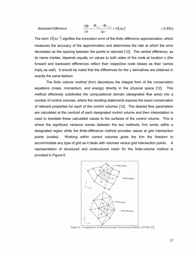
32

Backward Difference ( )xxx

jiji ΔΟ+Δ

Φ−Φ=

∂Φ∂ − ,1, ( 2.45c)

The term ( )nxΔΟ signifies the truncation error of the finite difference approximation, which

measures the accuracy of the approximation and determines the rate at which the error

decreases as the spacing between the points is reduced [12]. The central difference, as

its name implies, depends equally on values to both sides of the node at location x (the

forward and backward differences reflect their respective node biases as their names

imply as well). It should be noted that the differences for the y derivatives are obtained in

exactly the same fashion.

The finite volume method (fvm) discretizes the integral form of the conservation

equations (mass, momentum, and energy) directly in the physical space [12]. This

method effectively subdivides the computational domain (designated flow area) into a

number of control volumes, where the resulting statements express the exact conservation

of relevant properties for each of the control volumes [12]. The desired flow parameters

are calculated at the centroid of each designated control volume and then interpolation is

used to translate these calculated values to the surfaces of the control volume. This is

where the significant variance comes between the two methods; fvm works within a

designated region while the finite-difference method provides values at grid intersection

points (nodes). Working within control volumes gives the fvm the freedom to

accommodate any type of grid as it deals with volumes versus grid intersection points. A

representation of structured and unstructured mesh for the finite-volume method is

provided in Figure 6.

Figure 6. Comparison of Structured and Unstructured Meshes (FVM) [12]

33

Figure 7. Nomenclature for a Two-dimensional Control

Volume (FVM) [12]

2.1.8 Flywheel Overview

This section will be relatively basic as the underlying physical principles behind a

flywheel are extremely simple. The simplicity, lack of maintenance, and reliability are what

make it such a desirable means of energy storage. A flywheel is an inertial storage device

[45]. It absorbs mechanical energy by increasing its angular velocity and delivers energy

by decreasing its velocity [45]. An input torque will cause the flywheel speed to increase

while a load (output) torque will absorb energy from the flywheel, causing it to slow down

[45]. In the current study, a flywheel will receive the said input torque via a motor. More

specifically, a windmill will collect wind energy and direct it to the said motor which will

convert the energy into rotational, kinetic energy by increasing the speed of the flywheel.

The flywheel can then be decelerated at any time, turning the load torque into AC power

which can be distributed as needed. The flywheel is an invaluable addition to a wind

energy system, allowing for the storage of energy in times of excessive wind and the

distribution of the stored energy during periods of need. The major force of concern when

designing a flywheel is inertia, I .

34

Figure 8. Flywheel Geometry

The equations of motion for the flywheel, based on Figure 8, are listed below.

( ) ( ) 0,, 0 =−−=∑ θθθθθ ITTM ooiii ( 2.49)

Referring to figure four, iT is considered positive and oT negative, and whereθ andθ are

the first and second time derivatives ofθ , respectively [45]. Assuming the flywheel rotates

on a rigid shaft, equation (2.49) can be recast as shown:

( ) ( )ωθωθθ ,, oi TTI −= ( 2.50)

The kinetic energy of the flywheel is a fundamental relation between its moment of inertia

and its angular speed. The moment of inertia is given be equation (2.51b).

212i iE Iω= ( 2.51a)

2kmRI = ( 2.51b)

The variable k is known as the inertia constant and is equal to 21 for a solid cylinder or

disk [45]. Thus, it can be seen by equation (2.51a) that the change in kinetic energy over

given rotation ( 21 θθ → ). The corresponding change in kinetic energy is

( )11

2212 2

1 ωω −=− IEE . A coefficient of speed fluctuation is also given as equation (2.52):

ω

ωω 12 −=sC ( 2.52)

In the above equation, ω is simply the nominal average between the two angular

velocities. Finally, combining the previously defined elements, a final equation can be

reached to determine the change in energy from 21 θθ → .

212 ωICEE s=− ( 2.53)

35

Equation (2.53) is used to obtain the appropriate flywheel inertia corresponding to the

energy change 12 EE − [45]. Thus, it can be seen that the sizing of a flywheel is based on

a desired change in energy, the radius, angular speed, and the mass.

2.1.9 Pertinent Viscous Flows

The focus of this section is to describe a couple of common examples of viscous

flows having similar characteristics as a spinning disk. Two particular types of flow

systems, the plane Couette flow and Taylor-Couette flow, have been extensively studied

to examine laminar and turbulent patterns in fluids. The first type of viscous flow to

understand is known as Couette flow. In theory, the plane Couette system is arguably the

most straightforward fluid dynamical modeling system; experimentally, however, it often

presents the greatest challenge [52]. This particular type of flow is named in honor of

Couette (1890), who performed experiments on the flow between a fixed and moving

concentric cylinder to determine the viscosity of liquids [7], [11]. The most known

configuration of Couette flow is a theoretical set-up, consisting of two infinite parallel plates

(one moving and one stationary), and a zero pressure gradient. The two-dimensional,

Cartesian geometry of this particular flow along with the resulting velocity profile can be

seen in Figure 9.

Figure 9. Couette flow velocity distribution; bottom plat at rest, top

plate moving in x-direction at velocity = U [4].

This general problem allows the nature of viscosity and the no-slip condition to be

visualized. As mentioned in a previous section, no general analytic methods have

become available for the integration of the Navier-Stokes equations. However, the said

Couette flow is one specific case of a small group having valid solutions for all values of

viscosity. An important feature of Couette flow, with zero pressure gradients, is the linear

velocity distribution due to the no-slip condition present at both the stationary wall and the

moving wall. Going one step further, Couette flow with a pressure gradient has

36

importance in the hydrodynamic theory of lubrication [4] (as well as application to the

spinning flywheel). The flow in the narrow clearance between journal and bearing is, by

and large, identical with Couette flow with a pressure gradient [4]. In this case, the velocity

profile loses its linearity with the presence of a pressure gradient, adding complexity to the

flow by the appearance of vortices. In this case, a Fourier series can be implemented to

reach an exact solution. Thus, when analyzing the optimal design of gap spacing between

the flywheel and stationary walls, simplified Couette flow theory can be utilized for small

gaps; when the radius ratio approaches unity (discussed later in greater detail).

Now that two-dimensional Couette flow has been discussed, a progression in

complexity must be made to describe flow between concentric rotating cylinders. This will

require the Cartesian coordinates to be translated into cylindrical polar coordinates. In this

case where the inner cylinder is in motion and the outer cylinder is at rest affords an

example of an unstable stratification caused by centrifugal forces [4]. The fluid elements

nearest the rotating cylinder experience a greater centrifugal force and are propelled

outwards toward the stationary walls. This interaction of boundaries and forces on the

fluid particles result in a flow phenomena known as Taylor vortices, pictured in Figure 10

[4]. Figure 11 offers an enlarged, more detailed depiction of these toroidal vortices. In

figure eleven, it can be seen that counter-flowing groups of vortices exist stacked on top of

each other.

Figure 10. Taylor Vortices; inner cylinder rotating, outer

cylinder at rest [4].

37

Figure 11. Enlarged View: Taylor Vortices [30]

The stability of an inviscid fluid moving in concentric layers was initially studied by

the late Lord Rayleigh [21]. He made a very critical assumption that perfect slipping takes

place at the both the inner and outer cylindrical walls. He concluded that the flow is stable

if the liquid (confined between the cylinders) is initially flowing steadily with the same

distribution of velocity which a viscous liquid would have if confined between the two

concentric rotating cylinders (boundary layer flow). One set-back of his theoretical

deductions is that they applied only to flows when the motion is confined to two

dimensions (actual flow above/below a disk is represented by three-dimensional flow).

However, Rayleigh did create an analogy with the stability of a fluid with changing density

(compressible fluid) under the influence of gravitational forces. His analogy led to a further

conclusion that if the initial flow of the inviscid fluid is the same as that of a viscous fluid in

steady motion, the flow will be unstable when the two cylinders are rotating in opposite

directions [21]. In the case that they rotate in the same direction, then the motion is stable

or unstable based on whether 222Rω is greater or less than 2

11Rω , respectively. The

subscripts 1 and 2 represent the inner and outer cylinders, respectively. Rayleigh’s

criterion, shown below in equation (2.40), is applicable for determining inviscid rotational

instability [21]. Rayleigh stated, “an inviscid rotating flow is unstable if the square of its

circulation decreases outward” [21]. In other words, a given rotational flow is ensured if

equation (2.54a) holds true. Applying Rayleigh’s criterion to Couette flow between

cylinders, it can be reduced further to equation (2.54b) [7].

( )20d Rv

dr φ > ( 2.54a)

38

211

222 RR ωω > ( 2.54b)

Taylor improved a pre-existing stability criterion that Lord Rayleigh established in 1916 for

the scenario of both cylinders rotating. A criterion has been established to determine the

stability of this flow, known as the Taylor number, equations (2.55). Taylor simplified the

problem so that stability is dependent only on 12 ωω and a single parameter, now called

the Taylor number. For small clearance, ( )( )112 RRR <<− , the critical value for instability

is given by equation (2.55a) [20]. A classic paper by Taylor in 1923 showed that laminar

profiles are valid until a critical rotation rate is achieved, shown by equations (2.55) [20].

When this limit is exceeded, there appear stacked rows of toroidal vortices, now known as

the aforementioned Taylor vortices [4]. For the standard case where the inner cylinder

rotates and the outer cylinder remains at rest, the Taylor number can be calculated by

equation (2.41b).

( ) 17002

23

121 ≈−=νωRRRTa ( 2.55a)

3.412 ≥=

νωRdRT ea ( 2.55b)

An interesting note to this criterion is that the first appearance of these ring-like vortices at

the limit of stability (≥41.3) and the initial growth in amplitude of these waves does not

imply that the flow has become turbulent. The flow may surpass the Taylor criterion by a

large margin while remaining well-ordered and laminar, based on the system’s geometry

and angular velocity of the inner cylinder. In all, the Taylor number can be used to discern

three regimes of flow [4]. Table 2. Flow Regime Criterion base on Ta Number [4].

Flow Regime Taylor # Criterion laminar Couette flow Ta < 41.3

laminar flow with Taylor vortices 41.3 < Ta < 40 turbulent flow Ta > 400

A more in depth look at prior research of this flow type will be described in the following

section.

39

2.2 Previous Investigations The objective of section (2.2) is to explore previously conducted research in areas

pertaining to the parasitic drag analysis of a high-inertia flywheel rotating within a housing.

The flywheel rotating in an enclosure can essentially be thought of as a spinning disk

located co-axially within a stationary cylindrical housing (i.e. a rotating inner cylinder and a

stationary outer cylinder). Thus, the major emphasis of this project can be correlated to

past studies of a spinning disk. Rotating disks may be classified in two broad categories:

(1) “free disk,” a disk which rotates in a fluid mass of infinite extent and initially at rest; (2)

“enclosed disk,” a disk which rotates within a chamber of finite dimensions; the chamber is

considered to be fully closed so that only a finite volume of fluid is affected by the disk

notion [40].

More importantly, past skin friction and drag moment studies of a spinning disk will

be of particular value to help predict what will happen when the flywheel spins in an

enclosure. Any investigations that will improve the understanding of the flow involved in

this research will be advantageous. The reviewed research studies from the past have

both insightful aspects and imperfections. Each previous analysis will be closely detailed

in order to effectively determine which theories and methods correspond to the parasitic

drag study for an enclosed flywheel. Also, the majority of the reviewed studies in this

thesis are all correlated with one another; the most current workers have closely analyzed

the work of those before them to make necessary corrections to old solutions or to create

new, innovative solutions. As previously defined, the flow between a rotating inner

cylinder and a fixed outer cylinder is known as Taylor-Couette flow [16]. The historical

research presented in section (2.2) will be subdivided into three categories, based on the

method or approach utilized in each study: (1) experimental research, (2) theoretical

research, and (3) numerical research.

2.2.1 Experimental Research

The foundations of experimental research in fluid dynamics started in France and

England as early as the seventeenth century [14]. Thus, it seems logical to begin the

description of earlier research with what came first; experimental testing. Experimental

studies involving the analysis of flow imparted by a spinning disk have been completed by

many researchers. A variety of experimental apparatus and techniques have been utilized

40

over the years in attempts to better understand the effects of a disk rotating within a

viscous fluid. Although the objectives of this effort are not to complete experimental tests,

the results of others’ work might prove to be useful as a means of comparison of results

for both the theoretical and analytical drag analyses to be completed for the flywheel.

Dynamic similarity must be insured between past experimental models and the current

flywheel in order to compare results.

One of the earliest research trials was completed by Kempf in 1922 [17]. Kempf

measured the torque experienced by a disk rotating freely in air. The main emphasis of

his studies was the effects of surface roughness on the spinning disk. He tested various

surfaces (a fine paraffin surface, wood with a fine lacquer finish, and polished brass) at

Reynolds numbers between 1x104 and 2x106. The apparatus consisted of a disk which

was driven by a weight and pulley and torsion springs that measured the resulting torque

experienced by the disk. The experimental moment coefficients from Kempf’s

experiments can be seen in Figure 12 [18]. The three solid lines labeled numerically in

Figure 12 can be found as equations (2.44), (2.61b), and (2.65), respectively.

Figure 12. Turning moment on a rotating disk: curve (1) laminar, Sparrow and Gregg (2.44), (2) turbulent, von Karman (2.61b), (3) turbulent, Goldstein (2.65) [4]

Theodorsen and Regier [19] used experimental techniques to determine the

moment coefficient as a function of Reynolds number. They analyzed flow with Reynolds

numbers between 3.96x103 and 1.58x106 for a rotating disk [19]. They made a significant

discovery of extreme importance to the flywheel study that the skin friction does not

depend on the Mach number [40]. They ran tests with gases of different densities,

particularly air and freon in order to extend the range of the tested Mach numbers [19].

The research pair performed various experiments up to a Mach number of 2.7, giving

41

validity that compressibility issues are not a factor on the friction moment experienced by a

revolving disk [40].

They determined the moment on the disk at various angular speeds by linking the

horsepower required to revolve the disk at a specified rotational rate. The results of their

experimental work can be seen in Figure 12 of the next section. Theodorsen and Regier’s

measured results are also represented in Figure 17, as the “unfilled” circular, diamond,

and triangular data points. They are also the only pair of researchers described who

strictly evaluated compressible flow around a spinning disk.

Daily and Nece built a test rig with the option of interchangeable disks, to study a

variety of flow schemes around an enclosed disk. More specifically, they investigated the

usual disk-friction-torque measurements at different speeds, as well as pressure,

temperature, and velocity traverses in the liquid-filled spaces surrounding the disk [40].

They collected torque data over a range of Reynolds numbers from 103 to 107 for axial

clearance ratios as from 0.0127 to 0.217 for a constant small radial tip clearance

( ac =0.00637). Torque was measured by means of four strain gages bonded to the

rotating shaft driving the disk. Four SR-4 strain gages were placed at 45 degree angles

from the shaft’s centerline; the resulting bridge circuit registered torsional stresses only

[40]. Velocity and pressure data were obtained for both laminar and turbulent flows [40].

The team studied both edge effects and the viscous torque of the top and bottom of the

disk. When the flow in the thin annular gap between the cylindrical wall and the disk tip

was considered to be laminar, they assumed the presence of plane Couette flow, resulting

with a tip-friction torque coefficient given by equation (2.56) [40].

disk edge ωνπ

cabCM 2

4=′ ( 2.56)

They calculated the final value of MC , as used in the equations and plots, as the difference

between MC (gross), based on the total measured torque, and ′MC [40].

For turbulent flow, the annulus between the disk tip and the sleeve was treated as

a two-dimensional duct with no side-wall friction (an analogous circular pipe), leading to

the tip-friction torque coefficient labeled as equation (2.57) [40]:

disk edge abfCM 8

π=′ ( 2.57)

42

In the above equation, the value f is determined from the smooth-pipe curve from the

Moody diagram [40]. The theoretical coefficients for the disk’s edge will be discussed later

in this section.

A second innovative approach Daily and Nece utilized was to analyze the

interaction between the viscous moment experienced by both the spinning disk and the

stationary wall of the enclosure. The two researchers determined a set of moment

coefficients based strictly on empirical relations, shown below in equations (2.58a) through

(2.58d). These relations agreed with their entire range of experimental work to about 1

percent [40].

Regime I ( ) eM Ras

C π2= ( 2.58a)

Regime II ( )

21

10170.3

eM R

asC = ( 2.58b)

Regime III ( ) 4161080.0

eM Ras

C = ( 2.58c)

Regime IV ( )

51

1010102.0

eM R

asC = ( 2.58d)

The results of Daly and Nece’s experimental tests can be seen below in Figure 13.

Figure 13. Viscous torque on a disk rotating in an enclosure: Daily and Nece [40].

43

Nelka used a rotating disk apparatus in an attempt to simulate the high shear

stresses experienced by the hull of a full-scale ship [8]. He studied a disk diameter of two

feet, varying the surface roughness. He evaluated the performance of the rotating disk in

a tank (housing), in both mediums of air and water. He attached a dynamometer to the

shaft of the rotating disk and used a magnetic pickup-toothed gear configuration to

determine the angular velocity of the disk. He calculated the torque of the rotating disk as

a function of angular velocity. He fabricated the experimental test apparatus in such a way

that the disk could be tested both as a free disk and as a disk rotating in an enclosure [8].

A comparison of Nelka’s experimental moment coefficients of both an unbound and

enclosed disk can be seen in Figure 14.

Figure 14. Effect of Steel Housing on Torque due to a

Disk Rotating in Air: Nelka [8].

As originally expected, the disk rotating within a cylindrical enclosure experienced

less viscous torque when compared to a disk in unlimited space.

44

2.2.2 Theoretical Research

Many years after the first successful experimental procedures were conducted,

theoretical methods were introduced with hopes of reaching a more complete

understanding of fluid dynamics problems. In 1922, Taylor noted the following: All experiments so far carried out seem to indicate that in all cases steady motion is possible if

the motion be sufficiently slow, but that if the velocity of the fluid exceeded a certain limit,

depending on the viscosity of the fluid and the configuration of the boundaries, the steady

motion breaks down and eddying flow sets in. A great many attempts have been made to

discover some mathematical representation of fluid instability, but so far they have been

unsuccessful in every case [20].

In summary, Taylor observed the lack of correlation between theory and experiment. It

has been a consistent struggle over the years to provide mathematical representations of

fluid motion. Kelvin, Rayleigh, Sommerfeld, Orr, Mises, and Hopf (et al.) all investigated

the case in which the fluid is contained between two infinite parallel plates which move

with a uniform relative velocity (Couette flow). However, none of these researchers

extended their work into cylindrical coordinates to investigate Taylor-Couette flow.

However, in 1921, W.J. Harrison extended a method Orr previously used to determine (in

two cases) the highest speed of flow at which all small disturbances initially decrease.

Harrison found the maximum relative speed which two cylinders maintain in order that the

energy of all possible types of initial disturbances may initially decrease [20]. Harrison

assumed the motion of the flow to be only two-dimensional and his calculated value for

Reynolds criterion therefore contains only the relative speeds of the two cylinders [20]. (It

should be noted that at this point in time, it is denoted as Reynolds criterion because it had

not been successfully utilized to calculate the upper limit to the speed of flow that becomes

unstable i.e. the Reynolds number was not yet fully discovered and utilized as a means of

predicting laminar and turbulent flow) To summarize, the criterion is unaltered if the whole

system is uniformly rotated. Thus, his criterion is equivalent whether the inner cylinder is

fixed while the outer cylinder rotates, or vice versa [21].

von Kármán analyzed the flow about a disk rotating in a fluid initially at rest, for

both laminar and turbulent flow regimes [23]. von Kármán utilized an approximation

method based on the momentum equation [23]. He noticed that the peripheral velocity

falls from ωφ Rv = at the disk ( 0=z ) to zero at the edge of the boundary layer ( δ=z )

45

[23]. Thus, he assumed the variation of the tangential velocity component through the

boundary layer obeyed the th71

power law [23].

⎥⎥⎦

⎤

⎢⎢⎣

⎡⎟⎠⎞

⎜⎝⎛−=

71

1δ

ωφxRv

( 2.59a)

On the other hand, he also noticed that the radial velocity component rises from 0=rv at

the disk ( 0=z ) to a positive value 0>rv , and falls again to zero at the edge of the

boundary layer ( δ=z ) [23]. von Kármán’s resulting equation for the radial velocity can be

seen as equation (2.59b).

⎥⎦⎤

⎢⎣⎡ −⎥⎦

⎤⎢⎣⎡=

δδωα zzRvr 1

71

( 2.59b)

In equation (2.59b), the term α refers to the ratio of the radial shear stress components to

the azimuthal shear stress component. He based this assumption on previous results he

found while studying the characteristics of turbulent flow in smooth pipes [23]. von

Kármán, like many others, neglected the effect of the edge of the disk and focused solely

on the top and bottom sides. His resulting moment equations and moment coefficients for

both flow regimes can be seen in equations (2.60) and (2.61).

Laminar 2321484.12 ωρνRM = ( 2.60a)

Laminar 2168.3

eM R

C = ( 2.60b)

Turbulent ( ) 512250728.02 ωνρω ⋅= eRRM ( 2.61a)

Turbulent 51146.0e

M RC = ( 2.61b)

Figure 15 shows his theoretical viscous moment coefficients compared to the

corresponding Reynolds number (both are on logarithmic scales). The data points in

Figure 15 are from von von Kármán’s own experimental tests. The graph shows good

agreement between theoretical and experimental values for turbulent flow.

46

Figure 15. Viscous drag of a free disk: von Karman’s

theoretical calculations; laminar (2.46b), turbulent (2.47b)

However, there appears to be a discrepancy between theoretical and experimental values

for laminar flow. The results of von Kármán’s theoretical calculations can also be seen

compared to other researcher’s work in Figure 15. One limiting factor of von Kármán’s

theories however, is the neglect of the effect of friction on the cylindrical walls. Depending

on gap spacing, boundary layers are known to form on the housing walls, altering the flow

characteristics. Simply ignoring this fact could produce skewed results when determining

the moment coefficients.

Cochran [24] also investigated the laminar flow about a disk rotating in a fluid

initially at rest. A resulting moment equation and drag coefficient were also reached via a

power series. However, Cochran only used the power series to calculate solutions very

near the disk [24]. To obtain solutions as the vertical distance above the disk increases,

Cochran used an asymptotic series. He used matching principles to determine solutions

at intermediate distances above the disk’s surface. His results for laminar flow can be

seen below as equations (2.62a) and (2.62b) [24].

Laminar 23214616.02 ωνπρRM = ( 2.62a)

Laminar 2187.3

eM R

C = ( 2.62b)

Cochran also found an error in the von Kármán integration. His correction to the said

solution can be seen below in equations (2.63) [24]:

Laminar 2321469.12 ωνρRM = ( 2.63a)

47

Laminar 2138.3

eM R

C =

( 2.63b)

Cochran’s results, compared to the work of many other researchers, can also be seen in

Figure 18 of this section. Cochran completed his calculations under the assumption that a

radial pressure gradient was negligible. Past experimental research has proven the

existence of such a gradient which could leave room for error in Cochran’s solution.

Goldstein [35], [36] also analyzed the turbulent boundary layer of an unbound,

rotating disk. He manufactured an approximate moment coefficient based on the

logarithmic velocity-distribution law, listed below. The term *v is the friction velocity

( ρτ wv =* ), η is the axial distance from the surface of the disk, and u represents a free-

stream velocity ( ( )21 αω += RU ) [35].

Turbulent .log ** constvAvu e +=

νη

( 2.64)

Goldstein used the logarithmic velocity profile since von Kármán’s one-seventh-power law

method was only suitable for values of 600* ≤νηv . Through rigorous calculations,

Goldstein obtained the formula seen below, equation (2.65), to determine the torque

imparted on a rotating disk in turbulent flow [23].

Turbulent ( ) 3.0log97.11+= Me

M

CRC

( 2.65)

It is noteworthy that this equation has the same form as the universal pipe-resistance

formula. The numerical factors have been adjusted to obtain the best possible agreement

with experimental results. Equation (2.65) can be seen plotted, as curve three, versus

various theoretical and experimental data in Figure 16. Thus, von Kármán utilized a

power-law similarity formula, while Goldstein assumed a more general logarithmic

similarity law. A comparison of the power-law approach to the logarithmic approach can

be seen in Figure 16 (logarithmic scales for both the moment coefficient and the Reynolds

number).

48

Figure 16. Viscous drag of a disk rotating in unlimited space

(experimental data points: Schmidt and Kempf) [35].

Referring to Figure 16, for logarithmic values of the Reynolds number between

approximately 4.8 and 6.0, von Kármán’s theoretical method undershoots the

experimental data (data from experiments completed by Schmidt and Kempf) while

Goldstein’s calculated method undershoots the same experimental data points.

Concerning related topics, Granville derived a general logarithmic relation for the

resisting torque in an unbound fluid as a function of Reynolds number for arbitrary surface

roughness [39]. He obtained unique formulas for smooth surfaces, fully rough surfaces,

polymer solutions with a linear logarithmic drag-reduction characterization, and polymer

solutions with maximum drag reduction [39]. The previously documented analyses of von

Kármán and Goldstein are limited to smooth surfaces only. Also, Granville chose the

circumferential wall shearing stress as the reference shear stress in contrast to the

selection of the resultant wall shearing stress as chosen by both von Kármán and

Goldstein. Certain inconsistencies are thus avoided with this alternate reference selection

[39]. Equation (2.66) gives the resultant resisting moment coefficient for laminar flow [39].

Laminar 1 2

1.935 2M Me

k CR

= = ( 2.66)

Physically, the flow in the boundary layer is laminar starting at 0=R and undergoes

transition to turbulent flow at trRR = , specified by a Reynolds number of transition

treR [39]. Since Granville originally derived the logarithmic moment formulas for complete

49

turbulence over the entire disk, he developed a correction for the presence of laminar flow

in the central part of the disk [39].

Laminar

&

Turbulent

( ) ( ) ( )[ ]lamMturbM

e

eturbMM trtr

tr kkRR

kk −⎟⎟⎠

⎞⎜⎜⎝

⎛−=

25

( 2.67)

Granville’s resisting moment coefficient as a function of Reynolds number is given by

equation (2.68a). Equation (2.68b) gives the same relation for the case of maximum drag

reduction with a polymer solution.

Smooth

Surface ( ) 176.2log456.31

−= MeM

kRk

( 2.68a)

Polymer

Solution ( ) 44.32log33.111

−= MeM

kRk

( 2.68b)

The result of P.S. Granville’s moment coefficient calculation is plotted in Figure17.

Figure 17. Viscous drag of a disk rotating in unlimited space

(theoretical: von Karman, Granville, Goldstein; experimental values: Theodorsen/Regier, Hoyt/Fabula, Smallman/Wade) [39].

Figure 17 is important as it shows Granville’s results fall in between the theoretical values

determined by previous investigators. As previously mentioned, von Kármán’s method

overestimates the drag coefficient while Goldstein’s technique underestimates the same

value, when compared to experimental results. Thus, it can be seen in figure seventeen

50

that Granville’s logarithmic formula falls in between the two aforementioned moment

coefficients, ultimately giving better agreement to experimental measurements.

Dorfman [37], [38] studied the turbulent flow around an unbound, rotating disk. In

his work, he first presented a detailed compilation of past researchers’ work such as von

Kármán, Cochran, and Goldstein. Dorfman compared the effects of smooth and rough

surfaces on the resulting viscous torque of the disk [38]. He also conducted studies of air

cooling of gas turbine rotors by a radial flow [37]. More specifically, he looked at the effect

of friction resistance of a radial flow between a rotating disk and housing, also utilizing heat

transfer methods to study the cooling properties of said disk [37]. Dorfman, in the same

manner as Goldstein, used a logarithmic velocity distribution to find a moment coefficient.

Essentially, Dorfman extended Goldstein’s analysis to the special case of a disk with a

fully rough surface. His calculated moment coefficient for the smooth and rough surfaces

is represented by equations (2.69a) and (2.69b).

Turbulent: Smooth Surface

58.2)(log982.0 −= eM RC ( 2.69a)

Turbulent: Fully Rough

Surface ( ) 272.0108.0 RkC sM = ( 2.69b)

The constant sk in the previous equation is a friction factor based on the surface

roughness of the object under investigation. Figure 18 displays a collaborative

comparison between the studies of von Kármán, Cochran, Goldstein, and Dorfman [8].

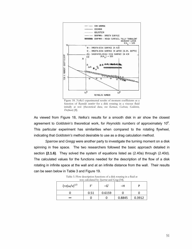
51

Figure 18. Nelka's experimental results of moment coefficients as a function of Reynolds number for a disk rotating in a viscous fluid initially at rest (theoretical data; von Karman, Cochran, Goldstein, Dorfman) [8].

As viewed from Figure 18, Nelka’s results for a smooth disk in air show the closest

agreement to Goldstein’s theoretical work, for Reynolds numbers of approximately 106.

This particular experiment has similarities when compared to the rotating flywheel,

indicating that Goldstein’s method desirable to use as a drag calculation method.

Sparrow and Gregg were another party to investigate the turning moment on a disk

spinning in free space. The two researchers followed the basic approach detailed in

section (2.1.6). They solved the system of equations listed as (2.40a) through (2.40d).

The calculated values for the functions needed for the description of the flow of a disk

rotating in infinite space at the wall and at an infinite distance from the wall. Their results

can be seen below in Table 3 and Figure 19. Table 3. Flow description functions of a disk rotating in a fluid at

rest; calculated by Sparrow and Gregg [34].

ζ=z(ω/ν)1/2  F'  –G'  –H  P 

0  0.51  0.6159  0  0 ∞  0  0  0.8845  0.3912 

52

Figure 19. Velocity distribution near a disk rotating in

a fluid at rest; calculated by Sparrow and Gregg [34].

Sparrow and Gregg’s theoretical calculations for the laminar case led to confirmation of

equation (2.62b), which is in agreement with the work of Cochran and Granville. The

theoretical drag moment calculated by the pair can be seen in Figure 21, labeled as curve

one. Their results show very close agreement when compared with experimental

measurements.

Schultz-Grunow noticed that research to date focused solely on the rotation of

disks in unlimited space and a lack of sufficient documents existed pertaining to the

rotation of disks within a housing [31]. Schultz-Grunow’s inspiration for studying this topic

arose when he discovered the presences of disk friction in turbo-machinery and rotary

machines [31]. He noticed that the rotating disks (he referred to them as wheels) were

narrow, and that the column expanse, s , (see Figure 20) was small in relation to the disk’s

radius [31].

Figure 20. Rotating disk in housing geometry: as used by F. Schultz Grunow [31].

53

Also, Shultz-Grunow, like many others, was not concerned with friction contributions from

the thin edge of the disk. He proposed the existence of three separate regions between

the rotating inner cylinder and the stationary outer cylinder: two boundary layers localized

on each wall and a core flow between them, as seen above in Figure 20 [31]. He

theorized that the core flow possessed an angular speed of approximately half of the

angular speed of the rotating disk. More specifically, he calculated a theoretical value of

512.0== RvK ωφ and measured the same ratio to be equal to 0.357 [31]. He

interpreted the discrepancy in values as a shear stress in the small radial gap between the

rotating disk and the housing wall, i.e., a small amount of torque produced by edge effects

of the disk [31]. The resulting theoretical laminar and turbulent moment coefficients from

Schultz-Grunow’s analysis are listed below as equations (2.70a) and (2.70b).

Laminar 2167.2

eM R

C = ( 2.70a)

Turbulent 51

0622.0

eM R

C = ( 2.70b)

Schultz-Grunow also completed experimental studies of a disk rotating within an

enclosure, discussed in more detail in the following section. Schultz-Grunow determined

momentum equations for the disk as well as the cylindrical housing. However, he

assumed a core flow existed between the two boundary regions which rotated at angular

velocity β . Thus, he too neglected the effects of friction caused by the housing walls

which could lead to discrepancies in his final solutions.

Schlichting attempted a moment coefficient for laminar flow in the case of small

axial gap spacing [4]. More specifically, for the case when the axial gap, s , is smaller than

the boundary layer thickness. He assumed in this case, the variation of the tangential

velocity across the gap becomes linear in the manner of Couette flow. Hence, the

shearing stress at a radial distance from the axis ( r ) is equal to srωμτ = [4]. Using this

relation for the shear stress, Schlichting determined the moment coefficient for the said

case, equations (2.71):

Laminar (small

axial gaps; s) eM Rs

RC 12π= ( 2.71a)

laminar (disk):

both sides 42M R sπω μ= ( 2.71b)

54

Equation (2.71a) is plotted as curve one in Figure 21, and shows good agreement with

past experimental values.

Figure 21. Viscous drag of disk rotating in a housing: curve (1) equation (2.71a), curve (2)

equation (2.70a), curve (3) equation (2.70b) [4].

Daily and Nece also fabricated theoretical expressions to verify their experimental

solutions. Their goal was to obtain equations to predict torque on an enclosed disk based

on the geometry of the system. Up until this point, all known researchers have considered

two regimes of flow (laminar and turbulent). Daily and Nece deciphered and classified four

different flow regimes within the enclosure. For the geometries

investigated ( )( )0.0127 0.217sa ∈ − , they determined that the mode of flow in the casing

depends only upon the Reynolds number and the geometry ( as ratio) [40]:

1. Regime I: Laminar Flow, Close Clearance. Boundary layers on the rotor and

stator are merged so that a continuous variation in velocity exists across the

axial gap, s .

2. Regime II: Laminar Flow, Separate Boundary Layers. The combined

thickness of the boundary layers on the rotor and stator is less than the axial

gap, s ; between the boundary layers is a core region in which no change in

velocity is expected to occur.

3. Regime III: Turbulent Flow, Close Clearance. The turbulent counterpart of

Regime I, for higher Reynolds numbers and turbulent flow on the circular

surfaces.

55

4. Region IV: Turbulent Flow, Separate Boundary Layers.

For a given as and a reasonable eR values, all four regimes may be possible over

a time period. In the past, various investigators have pointed out the existence of one or

more of these modes of flow; no single writer, however, has explicitly emphasized the

presence of all four and their limits of occurrence [40].

Their calculations provided additional verification for the simple close clearance,

laminar flow theory for friction torque in regime I, verifying the original value’s accuracy.

For regimes II, they chose a simple parabolic velocity distribution to represent relative

tangential velocities. A momentum analysis was performed of the von Karman type

refined to include cylindrical wall-friction effects to solve for the torque coefficients [40].

For regime III, the form of the variation of torque coefficient with eR was found to agree

with theoretical values, but the variation with as deviated slightly when compared to

theoretical predictions [40]. In the mode of regime IV, they used a one-seventh power-law

tangential-velocity distribution versus a logarithmic distribution to ease the numerical

process [40]. The resulting theoretical moment coefficients from past investigations of

Daily and Nece for all four flow modes can be viewed in equations (2.72a) through (2.72d).

Regime I ( ) e

M RasC π2

= ( 2.72a)

Regime II ( )1 2 ,Me

CC where C f s aR

= = ( 2.72b)

Regime III ( ) 41410622.0

eM Ras

C = ( 2.72c)

Regime IV ( )1 5 ,Me

CC where C f s aR

= = ( 2.72d)

Figure 22 offers a summary plot of these values at various as ratios. The plot covers the

as range of 0.01 – 0.20, and extends to values of eR which are experienced by all but the

most unusual applications [40]. The data of Figure 22 is represented by a logarithmic

scale; Daily and Nece deem the intersections of line segments for each geometry as an

indication of the existence of various regimes. This theory will be used to examine

influence of gap spacing for this flywheel study.

56

Figure 22. Delineation of flow regimes as studied by Daily and Nece [40].

Compared to experimental data, Daily and Nece deemed their theoretical MC -values for

Regime IV by approximately 17 percent for Reynolds number flows greater than 107, as

the 17 -power law (assumed for the velocity profiles) is no longer applicable [40]. It can

be seen that regime I exists for all as ratios as long as eR is kept sufficiently small. For

small values of as , regime II may never exist while at large values of as , regime III may

never exist. The experimental and theoretical investigations of Daily and Nece have been

explained in great detail in the previous two sections as their previous studies will prove to

be very useful when applied to the actual case of the rotating flywheel.

To this point, the previously mentioned theoretical studies have been concerned

with the flow above and below the rotating disk. These researchers all investigated thin

disk scenarios where edge effects were assumed negligible. The actual flywheel, having a

thickness of 0.9 meters, does not comply with the thin disk assumption. The viscous

forces experienced by the flywheel’s edge are predicted to be far too substantial to

neglect.

A major researcher of edge effects experienced by a rotating disk was Stuart [29]

in 1958. Stuart was successful in theoretically computing the flow pattern of the unstable

laminar flow in the presence of Taylor vortices while retaining the non-linear terms in the

57

equation of motion [4]. Stuart noticed that equilibrium exists between the transport of

energy from the base flow to the secondary flow as well as an existing equilibrium

between the viscous energy dissipation in the secondary flow [29]. The transfer of energy

from the base flow to the secondary flow causes a large increase in the torque required to

rotate the inner cylinder [29]. Thus, Stuart’s discovery has direct pertinence to the current

flywheel research. Figure 23 displays a comparison between Stuart’s theoretical moment

coefficient, Mc , to an experimental torque coefficient defined by equations (2.73).

Laminar (edge) 2 41 2MMC

R hπρω= ( 2.73a)

Laminar (edge):

small relative gaps

11

M aRd dc A A T

Rω

ν

−−⎛ ⎞= =⎜ ⎟

⎝ ⎠ ( 2.73b)

Turbulent (edge) Mc ~ 0.2aT − ( 2.73c)

In (2.45), the variable h represents the thickness, or height of the cylinder under

consideration.

Figure 23. Flow between two concentric cylinders; torque coefficient for

inner cylinder in terms of the Taylor number, Ta , from Stuart [4]

In Figure 23, Stuart’s results are compared to experimental results obtained by

Taylor [16]. It can be seen that good agreement exists between the theoretical and

experimental moment coefficients, indicating that the two sources can be considered

reliable for this study. The resulting moment coefficient derived by Stuart can be seen

below in equation (2.46), for gap spacing 028.0=Rd .

58

Schmeiden also studied the edge effects of a disk rotating in a housing. He made

an attempt to understand the influence of the radial gap between a rotating disk and

enclosure. However, his results only apply to low Re flows. He assumed creeping motion

(low Re flow) in order to significantly simplify the Navier-Stokes equations. Thus, his

theoretical efforts will only be applicable to the lower rotational velocities of this flywheel

study. His moment coefficient is dependent upon both the axial and radial gap sizes.

Laminar (edge) Me

KCR

= where 2K R sπ= ( 2.74)

The constant K depends on the two dimensionless ratios Rσ and s R (σ is the radial

gap dimension and s is the axial gap distance).

Dorfman also inspected the edge effects of a rotating cylinder. He reached an

equation that relates the moment coefficient of the top and bottom of the disk to that of the

edge [39]:

Laminar (edge) ( )( )1 2.5M

MCC

hR

′=

+ ( 2.75)

The term MC ′ represents the moment coefficient due to the disk and its edge, while

MC represents the moment experienced by the disk alone [39]. Substituting the

appropriate dimensions of the current flywheel gives the following

relation: 0.567M MC C ′= . According to Dorfman, the moment due to the disk faces is

approximately 57 percent of the total torque experienced by the said faces and the edge.

This presents a major divergence from many past theoretical and experimental studies;

much of the previous work focused on the rotation of thin disks. According to Dorfman’s

theories, the edge of the flywheel will produce 43 percent of the total torque experienced

by the flywheel. If Dorfman’s calculations are accurate, the drag due to the edge of the

flywheel will be as detrimental as the circular faces.

59

2.2.3 Numerical Research

As technology progresses, iterative solution techniques are being used more and

more via computational fluid dynamics. To analyze the flow of complex models, the math

can become too complicated. It is common to turn to numerical methods to help alleviate

some of the complexity involved in the solution procedure. For intricate differential

equations, the numerical method begins with an initial condition of a given variable and

then uses pertinent equations to determine the alterations of the said variable over a

period of time. This iterative procedure of recognizing variable changes over time is often

a good approximation method. This section is not restricted to the analytical research of a

revolving disk. Some of the literature reviewed was to broaden the knowledge of the

solution procedure for the drag analysis of a cylinder using computational fluid dynamics,

determining the criteria and resulting best choice for a turbulence model to analyze the

flow around a circulating flywheel.

Maleque and Sattar used numerical analysis to study the laminar convective flow

over a porous rotating disk. They studied the effects of variable properties (density,

viscosity, and thermal conductivity) on steady laminar flow and heat transfer for a viscous

fluid due to an impulsively started rotating infinite disk [41]. They implemented similarity

parameters to reduce the applicable system of governing equations to steady equations.

The resulting steady equations were solved using the Runge-Kutta and Shooting methods

[41]. Runge-Kutta methods are the most popular methods used in engineering

applications because of their simplicity and accuracy [42]. This method is used when

moving between node points on a grid system. The goal of the R-K method is to compute

an average slope (between current nodal position and desired nodal position) which will

make the aiming correct in order to get (shoot) to the target point along a straight line; the

most efficient path possible [42]. Due to the tedious and often numerous iterations, they

devised a computer program to reach the desired set of solutions. Maleque and Sattar

used a sixth-order R-K and Shooting method with step sizes of 0.001 to satisfy a

convergence criterion of 10-6 [41]. They determined the following radial and tangential

skin friction coefficients:

Tangential

( )( ) 211

0

eaf R

GC −+

′=

γ ( 2.76a)

60

Radial

( )( ) 211

0

eaf R

FC −+

′=

γ ( 2.76a)

The numerical results, along with a comparison of previously calculated results

(Kelson and Desseaux) are shown below in Table 4. Table 4. . Numerical values of the radial and tangential

skin friction coefficients (Maleque and Sattar) [41].

As seen in Table 4, their results show very close agreement to previous work.

He-yuan and Kai-tai numerically simulated axisymmetric, Couette-Taylor flow

between rotating cylinders for flow stability analysis [43]. To get to the desired system of

equations, they first introduced a stream function form of the Navier-Stokes equations for

simple Couette flow. Second, they determined the appropriate analytical expressions of

the eigenfunction of the Stokes operator in the cylindrical gap region and then proved the

said expressions orthogonal [43]. The spectral Galerkin approximation of Couette-Taylor

flow was then analyzed by introducing eigenfunctions of Stokes operator as the basis of

their dimensional approximation of subspaces. The results of their numerical simulation

indicated that when a small Reynolds number is used, the basic Couette flow is unique

and stable. They determined a critical Reynolds number of approximately 118, at which

the flow loses stability and initial Taylor vortices appear [43]. The appearance of Taylor

vortices at the corresponding eR can be seen in Figure 24.

61

Figure 24. Numerical simulation of Taylor Vortices (He-

yuan and Kai-tai) [43].

Their numerical simulation of flow instabilities show close agreement with experimental

results previously measured by Taylor [43]. Srinivasan, Jayanti, and Kannan investigated a computational fluid dynamics

based solution of the governing equations for the case of a rotating cylinder inside a

stationary cylindrical outer vessel filled with a fluid to determine the effect of Taylor vortices

on the flow field and heat transfer [44]. Their results confirm that the circumferential

velocity profile is a strong function of the Reynolds number and varies from a nearly

Couette-type flow at very low eR to a boundary layer like profile at high eR . All of the

research group’s numerical calculations were carried out using the commercially available

CFX 4.4 computer code. This program utilizes a finite volume method-based

discretization of the governing partial-differential equations on a non-staggered, structured,

body fitted grid [44] (all things to consider for modeling the flywheel in CFD). They utilized

the Rhie-Chow interpolation scheme, which ultimately eliminates the chequer-board type

oscillations of both pressure and velocity, often associated with the use of a non-staggered

grid [44]. They also used the SIMPLE method (Semi-Implicit Method for Pressure Linkage

Equations [12]) to couple the pressure and velocity. The discretization schemes for the

convection terms, diffusion terms, and the mass-fraction equation were solved using the

QUICK scheme, second-order central differencing scheme, and the SUPERBEE scheme,

respectively [44]. For the QUICK scheme, a quadratic approximation is introduced across

two variable points at the upstream and one at the downstream depending on the flow

direction [12] (see Appendix B of reference [12] for a detailed example of the QUICK

scheme). The SUPERBEE scheme incorporates the total variation diminishing (TVD)

property which eliminates oscillations commonly associated with higher order differencing

62

schemes [44]. The aforementioned discretization schemes will all be valid selections

applicable to the flywheel study.

Srinivasan, Jayanti, and Kannan used a structured, orthogonal grid for the two-

dimensional flow domain which contained a total of 9,600 cells. Since they did not know

the precise location of the Taylor vortices a priorí, they implemented uniform grid spacing

in the axial location [44]. In order to compensate for strong velocity and mass fraction

gradients in the radial direction, they used an expanding grid [44]. Once they tested for

grid independence, they computed velocity profiles near the inner cylinder to compare

three radial geometries in which the grid spacing near the wall was successively reduced

by a factor of two [44]. The main goal of their work was to determine the mass-transfer

coefficient, which is not entirely applicable to the current flywheel study. However, they did

model and simulate the same type of flow as in the flywheel investigation, offering some

useful insight on discretization schemes and grid structure. Also, they examined the effect

of the radius ratio (gap spacing) by plotting the dimensionless tangential velocity in terms

of the dimensionless radial distance for different radius ratios. They determined that for

small gap widths, the radial profile of the circumferential velocity is nearly linear (Couette

flow) while for increasing gap widths, the non-linearity characteristics begin to appear

(Taylor vortices).

Miyazoe et al. used CFD to establish an efficient design process for a centrifugal

blood pump [13]. In order to achieve their goals, they implemented flow visualization

experiments to validate known flow patterns and hemolysis tests to prove the analysis is

necessary [13]. They utilized the ε−k method, a widely used turbulence model and

logarithmic velocity functions at the locations very near the wall [13]. They divided the flow

domain into three sections: inlet passage, pump part, and diffuser having 1,600 nodes,

127,920 nodes, and 4,800 nodes, respectively [13]. Since shear stress is considered as

one of the major causes for destruction of red blood cells, the main concern of their study

was to locate regions of high shear stress [13]. They used various particle tracking and

velocity vector options in CFD to obtain a visual depiction of the flow in the centrifugal

pump. CFD analysis indicated that a change to a smaller radial gap greatly affected the

shear stress of the fluid, locating high concentrations near the cylindrical wall as the radial

gap spacing decreases.

These numerical studies from past investigators will be considered when using

CFD techniques to analyze the flow around the flywheel. Maleque and Sattar’s numerical

results can be used as a different method in which the skin friction of the flywheel can be

63

calculated. Srinivasan, Jayanti, and Kanna’s methods will be considered when utilizing

CFD to analyze the drag experienced by the flywheel. In particular, the specific

discretization and grid generation techniques used in their studies will be considered and

applied when necessary to the current flywheel study. Finally, Myazoe et al. CFD study

will also be regarded when employing computational methods to the current flywheel drag

analysis.

64

C H A P T E R 3 : M E T H O D O L O G Y

The main objective of this effort is to provide a complete parasitic drag analysis

experienced by a high inertia flywheel rotating in a housing. When solving any type of

problem, especially a complex engineering problem, it is advantageous to develop a

systematic approach to reach a solution. Following a systematic approach promotes

organization and can provide a better overall understanding of the task at hand. Moran

and Shapiro [28] offer a five step problem solution method that will be followed in this

section in order to effectively outline the procedures followed, guiding the reader through

the flywheel drag analysis.

A general synopsis of the five steps, fully documented in reference [28], is listed as:

1. Known: State briefly what is known

2. Find: State concisely what is to be determined

3. Schematic and Given Data

4. Assumptions: Form a record of how you model the problem and list all

simplifying assumptions and idealizations

5. Analysis: Reduce appropriate governing equations and relationships to forms

that will produce the desired results

Thus, this chapter will first illustrate the steps that will be taken to complete a parasitic drag

analysis of the revolving flywheel. Next, the chapter will provide a section that describes

the methodology used to effectively model the problem using computational fluid

dynamics. Also, CFD techniques will be utilized to explore the effects of gap sizing

between the rotating flywheel and stationary enclosure.

3.1 Theoretical Drag Methods This section will document the procedures used to analyze the parasitic drag of a

flywheel with both theoretical and computational methods. The rotating flywheel problem

will be solved in various fashions, computing the drag of an unbound flywheel and a

flywheel rotating within an enclosure. This comparison will be used as evidence that

locating a rotating flywheel inside a right cylindrical enclosure will be beneficial as it

reduces the overall drag experienced by the flywheel; as well as improving the energy

system’s factor of safety by preventing direct human interaction. Various theoretical

methods from past researchers will be utilized for each scenario (unbound versus

65

enclosed) in an attempt to obtain an accurate viscous drag moment of the flywheel. The

five step solution method previously mentioned will be followed to strictly document each

drag analysis. The parasitic drag of an enclosed flywheel will calculated at a range of

pressures from one atmosphere down to one-twentieth of an atmosphere. The lowering of

the pressure will be used to simulate the evacuation of the cavity between the flywheel

and housing as a vacuum pump could. This calculation will be used to determine the

feasibility of a low-pressure, drag-reduction system. Finally, CFD will be used to offer

visual support of the flow phenomena around an enclosed flywheel as well as a design

tool to determine optimum gap spacing between the flywheel and housing.

As a starting point, the problem will be solved initially as a “free disk”. The

terminology “free disk” infers that the disk will rotate in open space, free of any boundaries.

This simplified form of the drag analysis is expected to produce a viscous moment that is

of the same order of magnitude as with a disk rotating within a housing would expect. The

moment calculated in this preliminary study will be used to rationalize the initial prediction

that a disk rotating in a housing will experience less frictional drag when compared to a

disk spinning without boundaries. This prediction is based solely on the comparison of

moment coefficients between of a disk rotating in different environments. More

importantly, it will justify the prediction that locating the working flywheel within an

enclosure will be the first effort to reduce the drag moment, increasing the energy system’s

overall efficiency. Following the five step solution method [28], the known data for

concerning the flywheel can be found in the following tables. The approximate physical

properties of air are given below in Table 5 [3]. Table 5. Physical properties of Air at Standard Atmospheric Pressure [3]

P  T  ρ μ υ R γ

kg/m2 = Pa   K  kg/m3  N‐s/m2  m2/s    KkgJ ⋅   ‐‐‐ 

101325  288.15  1.223  1.79E‐05  1.46E‐05  2.87E+02  1.4 

Table 6 specifies the geometrical parameters of the flywheel. The listed angular speed of

the flywheel corresponds to its maximum operating speed, an equivalent of 1,000

revolutions per minute; the rotational speed at which the maximum viscous torque will be

produced. The friction moment will be calculated for the flywheel at rest up to said

maximum angular speed to determine the approximate angular velocity at which the

viscous moment becomes detrimental to the operating efficiency of the system.

66

Table 6. Flywheel Parameters Description  Symbol  Value  Units 

 diameter  d  5.9  m 

radius  R  2.95  m 

thickness  t  0.9  m 

angular velocity range  ω [0 ‐ 104.72]  rad/s 

A schematic of the unbound rotating disk can be seen in Figure 2 of section (2.1.1). The

flow pattern, as a result of the rotation of the disk, can also be visualized in the same

figure. Due to the size of the flywheel, all three flow regimes (laminar, transition, turbulent)

will be present at angular speeds greater than five radians per second. At the current

time, the moment coefficients determined by past investigators are unique only to laminar

and turbulent flow; the transition zone is treated as a demarcation line rather than an

actual region. Thus, for the scope of this study, the transition region will be ignored,

focusing specifically on a laminar region and a turbulent region. Unless otherwise noted,

the flow will be assumed to transition from laminar to turbulent flow at a Reynolds number

of 3x105 [4]. Therefore, equation (2.4) can be used to determine the transition radius on

the disk, deciphering between the two regions present on the circular top and bottom

surfaces of the disk. This calculated transition radius will be used for all scenarios in this

theoretical drag analysis. The total turning moment on the flywheel will be found by

subtracting the critical turbulent moment (acting from 0R = to the critical radius trR R= )

from the total turbulent moment and then adding the laminar moment that occurs over the

said critical area:

( 2.95 ) ( ) ( )tr trTotal turb R m turb R R lam R RM M M M= = == − + ( 3.1)

The final moment equation listed above is based on the theoretical methodology of

Granville [39]. The viscous moment coefficient to be used in equation (3.1) will be

determined using various methods. The theoretical equations determined by past

investigators will be one scheme for determining drag coefficients. Some methods of past

investigators will have to be combined in order to fully analyze the friction resistance of the

entire flywheel. For example, von Karman only determined a moment coefficient for the

circular top and bottom surfaces on a rotating disk. Therefore, his efforts will have to be

combined with other’s to include parasitic drag contributions due to edge effects.

Experimental data from earlier studies will be another technique to determine the

said coefficients. Finally, a combination of the two methods will be a third scheme to

67

determine frictional losses. More specifically, experimental data will be input into the

logarithmic equations derived by Goldstein and Granville to predict friction coefficients.

Implementing diverse methods as mentioned should offer an accurate portrayal of the

aerodynamic forces experienced by the flywheel.

Microsoft EXCEL will be utilized in order to make the aforementioned calculations

at a range of angular speeds and pressures. Basic “if” statements will be used in EXCEL

to apply the appropriate conditions and determine the resulting friction moment. Iterations

will be made at various angular speeds of the flywheel, with a step size of one radian per

second. The results can then be compared to experimental data of earlier studies.

3.2 Numerical Drag Methods / Optimal Gap Design The prediction of skin friction on the surface of a body in an attached flow is nicely

accomplished by means of a boundary layer solution coupled with an inviscid flow

analyses to define the flow conditions at the edge of the boundary layer [1]. This well-

developed approach is often too complex and tedious to carry out by hand. However,

many commercial CFD programs have the ability to rapidly carry out the desired

calculations. Although these advanced computer programs can quickly produce results,

an important consideration is the accuracy of the said results. More specific to the

flywheel problem, the accuracy of the CFD Navier-Stokes equations used to determine

skin-friction and heat transfer must be investigated. The need to have a very closely

spaced grid in the vicinity of the wall, uncertainty in the accuracy of turbulence models

when turbulent flow is being calculated, and the lack of ability of most turbulent models to

predict transition (from laminar to turbulent) are three definite aspects that tend to diminish

the accuracy of Navier-Stokes solutions [12].

However, since the present flow about a rotating flywheel does not experience

separation at any point, the use of boundary layer solutions for skin friction and

aerodynamic heating is an advantageous approach that will be used. Also, the following

CFD procedures will only be used for the scenario of the flywheel rotating within a housing

to help visually depict the flow phenomena and characteristics involved in this study. It

should be noted that CFD will be used only to seek trends in the flow; the computational

simulations do not exactly imitate and thus, actual flow parameters will not be obtained

from the flow. The unbound flywheel is a more trivial problem and will not be analyzed

with CFD methods. The following geometries of the flywheel and enclosure combination

will be investigated. The terms s and c denoted the axial and radial distances from the

68

flywheel to the housing, respectively. These dimensions were determined considering two

parameters: (1) boundary layer thickness and (2) staying within the s/a ratio range tested

by Daily/Nece so that their results could be used as a means of comparison. The

boundary layer thickness on the top and bottom face of the flywheel, at maximum angular

velocity, was calculated to be approximately 4.1 centimeters ( 1 50.522( )δ ν ω= by von

Karman and 2 1 50.526( )Rδ ν ω= by Goldstein). Thus, the spacing of 0.0826 meters is

used to leave a gap between the boundary layers expected to form on the flywheel and

the ceiling/floor of the enclosure. Housings one and two are designed to have separated

boundary layers in the axial direction. Housing numbers 3 and 4 are intended to provide

separated boundary layers with a much greater “core” region. Housing numbers 5 and 6

are implemented to have merged boundary layers in an attempt to analyze changes in

velocity and pressure as the flywheel rotates. Table 7. Gap spacing schemes examined using CFD

Housing # Axial Gap: s (m.) Radial Gap: c (m.) 1 0.0826 0.0826 2 0.0826 0.018792

3 0.64015 0.64015

4 0.64015 0.018792

5 0.037465 0.037465

6 0.037465 0.018792

The angular speed of the flywheel will be manipulated along with the scenarios in the

above table in an attempt to achieve the four flow regimes discussed by Daily and Nece in

a previous section of this report. The gap spacing chosen are based on the experimental

studies of the previously mentioned research team. The as / ratio range of 0.0127 to

0.217 was applied to the flywheel dimensions ( mR 95.2= ) so that proper comparison to

the experimental results of Daily and Nece could be achieved. The velocity profiles and

pressure distributions through the varying gap spaces will be examined to determine the

effect, if any, the axial and radial gaps have on the flow around the flywheel.

A legitimate starting point is to discuss the pre-process setup of the flywheel CFD

analysis. The flywheel simulation will first be modeled in GAMBIT, version 2.4.6. The flow

about a rotating flywheel in an enclosure can be considered axisymmetric flow. More

specifically, the azimuthal flow about the z-axis does not change at any given radial

distance ( 0φ∂ ∂ = ). Thus, the flow can be modeled as two-dimensional which will greatly

simplify matters and ultimately shorten computation time by reducing the extent of the

69

computation model to a symmetric subsection of the overall physical system [47]. For two-

dimensional axisymmetric problems, the rotation does not need to be defined; the rotation

will always be about the x-axis by default, with the origin at (0,0) [47]. The flow will be

modeled as two-dimensional, axisymmetric swirl flow (setting found in the Solver panel).

This setting effectively activates the solution of the momentum equation in the

circumferential direction [48]. Remember, the axisymmetric assumption only implies the

absence of circumferential gradients; non-zero circumferential velocities can and will

appear in this flywheel study. Despite the fact that this study concerns a flywheel rotating

about a vertical axis, it will appear to be revolving around the horizontal x-axis when first

modeled. However, this orientation will not in any way skew the results; gravitational

effects will still be oriented in the proper direction. Once the outline of the figure is drawn,

a mesh will be applied to divide the computational domain into cells (elements). This

constitutes one of the most important steps during the pre-process stage [12]. For each

geometry, a structured mesh will be applied, using sub-mapping, mapping, quad-element,

and tri-element variances. Also, a boundary layer mesh will be applied to the surfaces of

the flywheel as well as on the enclosing walls. This places a heavy concentration of nodes

in locations where viscosity has the greatest effect. By increasing the number of cells (i.e.,

with decreasing mesh spacing) in the computational domain geometry, the accuracy of the

solution is usually enhanced [12]. The order of the mesh generation goes as follows: (1)

boundary layer mesh, (2) edge mesh, (3) face mesh. The geometry and mesh of housing

number 1 (see Table 6) can be seen below in figure 25. The flywheel, chamber, and

housing will be meshed using different methods to assist in checking for accuracy. For the

first method, the geometry will be divided into three separate faces (Figure 25), meshing

each face individually. Also, the entire region will be kept as a single, open face and then

meshed appropriately. A zoomed in view of the mesh using the first of the aforementioned

methods can be seen in Figure 26. The coarser grid near the wall represents the

approximate region where the boundary layer is expected to inhabit. From experience,

anywhere from five to ten nodes need to be placed across the boundary layer mesh to get

optimum simulation results.

70

Figure 25. Geometry of flywheel, computational

domain, and enclosing walls (3 faces)

Figure 26. Structured, boundary layer mesh

The flow being modeled will be considered steady, viscous flow. This will eliminate any

time-dependence variables in the governing equations. The flow will be simulated with

various turbulence models for a compressible gas. Setting the fluid type to ‘ideal gas’ will

include compressibility effects into the calculations; for compressible flows, the ideal gas

law is the appropriate density relationship [47]. The input of the operating pressure is of

great importance when you are computing density with the ideal gas law. Equation (3.2)

notes that the operating pressure is added to the relative pressure field computed by the

solver, yielding the absolute static pressure.

71

Op

w

P PR T

m

ρ+

= ( 3.2)

The appropriate density and viscosity (materials menu) will be set under material

properties corresponding to the operating temperature. The boundary conditions are set

so that the designated flywheel section of the two-dimensional geometry is a rotational

surface. Simulations will be executed at a range of angular velocities, with a maximum

speed of 104.72 radians per second (the default units used by FLUENT for angular

speed). The outer walls of the geometry will be set to stationary walls while the two small

lines connected to the x-axis will be set as an ‘axis of symmetry’. Taking advantage of the

symmetric geometry of this problem will greatly reduce computation time.

Now that the pre-process steps have been identified, the CFD solver procedures

will be outlined. There are many difficulties associated with solving compressible flows;

mainly, complexity arises as a result of the high degree of coupling between the velocity,

density, pressure, and energy [12]. The said coupling leads to instabilities in the solution

process and often needs unique techniques to reach the desired, converged solution. In

all cases, the initial solution will be found at a reduced angular velocity as a laminar flow

model. This will give a good initial guess with the intent that will ultimately allow for

turbulence model solutions to converge at a more rapid pace.

Each scenario will be modeled at a specific angular speed which will remain

constant until a solution is reached. Since the modeled flows will not be time dependent,

an operating pressure will be used versus a floating-point pressure function. However, the

operating pressure is less significant for higher-Mach number compressible flows [47].

The pressure changes in said flows are much larger, eliminating the need to use gauge

pressures. Since FLUENT always uses gauge, the operating pressure can be set to zero,

making gauge and absolute pressures equivalent ( gaugeoperatingabs PPP += ) [47].

For scenarios one and two (housing one and housing two), a variation of

turbulence models will be used to visualize the flow and examine the spacing of the

enclosing walls. Once grid independence has been established amongst the various

enclosure geometries, a normalized viscous moment will be graphed versus the number of

cells used in the mesh to prove grid independence has been reached. It should again be

noted that the CFD simulations are not intended to strictly imitate the exact flow around

the flywheel. Instead, it will be used to provide a means to visualize the flow around the

flywheel amongst the varying gap sizes. The turbulence model which produces the most

72

comparable results when compared to experimental and numerical results of the past will

be deemed the most beneficial for the purpose of viewing images of previously mentioned

flow phenomena. Once a beneficial turbulence model has been selected, the said model

will be used to simulate the flow in the remaining four housing geometries: housing

numbers 3 through 6; Table 6).

No single turbulence model is universally effective at reaching solutions for all

types of problems. The choice of turbulence model will depend on considerations such as

the physics encompassed in the flow, the established practice for a specific class of

problem, the level of accuracy required, the available computational resources, and the

amount of time available for the simulation [48]. Thus, both the abilities and limitations of

each model must be factored in the decision of which model will best suit the simulation of

flow around the flywheel.

There are two computational methods to consider when picking a turbulence

model: (1) RANS – Reynolds Averaged Navier-Stokes and (2) RSM – Reynolds Stress

Model. The Reynolds-averaged Navier-Stokes equations govern the transport of the

averaged flow quantities, with the whole range of the scales of turbulence being modeled.

The RANS-based modeling approach therefore greatly reduces the required

computational effort and resources, making it a desirable approach for the flywheel

analysis [48]. In Reynolds averaging, the variables in the Navier-Stokes equations are

classified into mean and fluctuating elements:

i i iu u u′= + ( 3.3)

In equation (3.3), the terms iu and iu′ represent the mean and fluctuating velocity

components, respectively. The same principle is applied to all scalar properties such as

pressure ( i i iφ φ φ′= + ) and these manipulated variables are substituted into the Navier-

Stokes equations accordingly. When applying RANS, there are three turbulence models

to choose from: (1) Spalart-Allmaras (SA), (2) k ε− , and (3) k ω− . In the case of the

Spalart-Allmaras model, an additional equation is added to the existing governing

equations which represent the turbulent viscosity. The SA model is thus known as a ‘one-

equation’ turbulence approach. The k ε− and k ω− turbulence models are known as

‘two-equation’ models, as they invoke two additional transport equations. The additional

variables introduced by these models are turbulent kinetic energy ( k ), turbulence

dissipation rate (ε ), and the specific dissipation rate (ω ).

73

The alternative approach to Reynolds-averaging is the full Reynolds stress model

(RSM). The RSM is the most elaborate turbulence model that FLUENT provides [48].

The RSM accounts for the effects of streamline curvature, swirl, rotation, and rapid

changes in strain rate in a more rigorous manner than one-equation and two-equation

models, and has greater potential to give accurate predictions for complex flows [48]. The

Reynolds stress method closes the Reynolds-averaged Navier-Stokes equations by

solving transport equations for the Reynolds stresses, together with an equation for the

dissipation rate. To prove the complexity of the model, the additional variables require the

addition of five transport equations (seven additional equations for three-dimensional flow),

making it otherwise known as a ‘five-equation’ model.

Once an efficient turbulence model is selected, further tests must be completed to

establish grid independence; more specifically, an evaluation of the numerical uncertainty

(i.e., accuracy) within the simulation is necessary. It is important to recognize the fact that

a converged solution does not necessarily indicate an accurate solution [12].

Convergence of a numerical process can be stated as the solution of the system of

algebraic equations approaching the true solution of the partial differential equations

having the same initial and boundary conditions as the refined grid system; this type of

convergence is more formally known as grid convergence or grid independence [12].

Some prevalent sources of error when dealing with numerical solutions include:

discretization error, round-off error, iteration/convergence error, physical-modeling error,

and human error [12].

A second type of convergence is known as iterative convergence. There are three

important aspects to abide by to reach iterative convergence: (1) the discretized equations

(momentum, energy, etc.) are deemed to converge when they reach a specified tolerance,

(2) the numerical solution no longer changes with iterations, and (3) overall mass,

momentum, energy, and scalar balances are obtained [12].

The recommended procedure that will be used for estimation and reporting of

discretization error is the Richardson Extrapolation (RE) method [53]. The first step is to

identify a single cell, mesh, or grid size (h) that can be followed through the error

estimation procedure.

1 2

1

1 N

ii

h AN =

⎡ ⎤= Δ⎢ ⎥⎣ ⎦∑ ( 3.4)

74

Equation (3.4) gives the area of concerned cell ( iAΔ ) and the total cell count of the

corresponding refined mesh ( N ). This equation is to be used when integral quantities are

considered [53]. Thus, in this flywheel study, the appropriate integral quantity that will be

followed is the viscous moment. For this method, the grid being inspected must be refined

a minimum of two times, giving a total of three different meshes to compare. It is critical to

refine the grid in a structured manner; the use of geometrically similar cells is preferable

[53]. Next, the order ( p ) of the concerned property must be determined; as mentioned,

the property to be tracked in this study will be the overall moment about the flywheel’s axis

of rotation. The following equations will be used to determine the order [53]:

32 2121

1 ln ( )ln( )

p q pr

ε ε= + ( 3.5a)

21

32

( ) lnp

p

r sq pr s

⎛ ⎞−= ⎜ ⎟−⎝ ⎠

where ij i jr h h= ( 3.5b)

32 211*sin( )s ε ε= where ij i jε ϕ ϕ= − ( 3.5c)

Equations (3.5) can be solved by using fixed-point iteration, with the initial guess being

equal to the first term of equation (3.5a) [53]. It should be noted that the term ϕ denotes

the solution of each grid; ( 1ϕ is the moment solution of grid one, etc.). Next, the

extrapolated values, approximate relative error, and the extrapolated relative errors will all

be calculated [53]:

2121 1 2 21( ) ( 1)p p

ext r rϕ ϕ ϕ= − − ( 3.6a)

21 1 2

1ae ϕ ϕ

ϕ−

= ( 3.6b)

12

21 112

extext

ext

e ϕ ϕϕ

−= ( 3.6c)

Finally, the previously calculated values from equations (3.5) and (3.6) are summoned to

determine the fine grid convergence index:

21

21

21

1.251a

fine p

eGCIr

=−

( 3.7)

For this study, a convergence criteria of three percent was chosen as the determining

factor whether a grid had reached independence.

75

Now that grid independence has been established, the mesh can be used for each

simulation as the turbulence model is changed. Once the grid has reached independence,

the model must be checked for iterative convergence. To assess iterative convergence,

converged solutions will be obtained when the absolute convergence criteria is set to both

103 and 104. The approximate relative error will be checked between the two solutions,

making sure no significant change in solution has occurred (again, a criterion of around

three percent was used for comparison). If there exists more than a three percent

difference between iterations, the order of convergence will be continually increased by an

order of one until the criteria is satisfied. Also, to seek further accuracy, each solution will

be obtained using first and second order discretization techniques.

The results of the CFD simulations will have multiple applications. The major

purpose for the computational drag analysis was to be used as a means of comparison for

the theoretical parasitic drag analysis completed on the enclosed flywheel. In the best

case scenario, the numerical calculations will show close agreement to theoretical results.

As in the analytical portion, the effects of the viscous moment as a result of pressure

reduction will be examined. Finally, CFD will be used to examine the effects, if any, of

varying the gap size between the flywheel and housing in the axial and radial directions. If

the said spacing has a noticeable effect on the drag-moment, the optimal housing design

for the designed flywheel will be sought. Plots from the CFD solutions will be examined in

an effort to look at boundary layer reactions as a function of gap size; the interaction of the

viscous layer formed on the flywheel with an opposing layer formed on the enclosure.

76

C H A P T E R 4 : R E S U L T S

The theories and methodology described in previous section was applied to the

current flywheel study. The main objective of this study was to conduct a theoretical,

parasitic drag analysis of a current flywheel. Thus, the first section in this chapter will

present the calculated drag moments based on past theoretical research. The resulting

friction moment is shown for both an unbound and enclosed flywheel for comparison. The

said drag moments will then be presented as a function of varying pressure to determine if

a reduced pressure system is worth investigating. The computational results will then be

compared to theoretical work. Finally, the CFD simulations will be analyzed and

compared to theoretical values in an attempt to determine optimal gap spacing in both the

axial and radial directions between the flywheel and housing. The CFD simulations will

also serve as a means to depict various flow phenomena around the flywheel such as

boundary layers and Taylor Vortices.

4.1 Theoretical Results As described in the methodology section, the drag of the specified flywheel was

first calculated at atmospheric pressure for two scenarios: (1) rotation in free space and (1)

rotation inside an enclosure. The moment coefficient at corresponding Reynolds numbers

was found using various theoretical approaches from earlier researchers; theories from the

past were applied to the current flywheel study in an attempt to accurately predict the

viscous moment it will experience at maximum rotational speed. The results, compared to

experimental data from past work, can be seen in the figures (27-30). The experimental

values used in this thesis were collected from past studies of spinning disks and rotating

cylinders. Compressibility effects appear to be limited as was first discovered by

Theodorsen and Regier; this can be verified in Figure 12 (Chapter 2) as the different

theoretical methods (based on incompressible assumptions) closely agree with test data

collected at a Mach number range of 0.29 to 1.69. These Mach numbers correspond to

approximate, flywheel operating speeds between 30 and 200 radians per second (rps),

respectively. The maximum rotational speed of the flywheel is 105 rps. Thus, based on

experimental and theoretical comparison, the maximum operating speed of the flywheel

falls in a range where compressibility effects can be ignored for this preliminary drag

analysis. Past experimental values determined by Kempf, Schmidt, Daily and Nece, and

Zumbush are also used as a means of comparison for various scenarios and can be seen

77

in Figure 27 through Figure 34. It should be noted that Figures 27 through 32 represent

the moment coefficient for the top and bottom surface of the flywheel only. The

experimental values in the same figures strictly correspond to these surfaces as well.

Additional viscous friction will be present as a result of edge effects.

4.1.1 Unbound Flywheel

This section examines the friction moment experienced by the flywheel while

rotating in free space. This calculation approximates the viscous moment of the flywheel

as if it were operating above ground, open to the atmosphere (neglecting atmospheric

influences). The moment coefficient was calculated as a function of the Reynolds number;

the coefficients plotted in Figure 27 represent the laminar flow regime. All methods

described in Chapter 2 were applied to this flywheel analysis. The theoretical methods

included in this section were selected based on agreement to past experimental data.

Also, this section pertains to the calculation of the viscous moment coefficient of the top

and bottom surfaces of the flywheel only; the contribution to the total friction drag by the

edge of the flywheel will be discussed in a following section.

von Karman

Cochran/Granville

Dorfman

Sparrow and Gregg

0.006

0.007

0.008

0.009

0.010

0.011

0.012

0.013

0.014

0.015

0.016

5.0E+04 1.0E+05 1.5E+05 2.0E+05 2.5E+05 3.0E+05log Re

CM

Kempf (experimental)

Schmidt (experimental)

Theodorsen and Regier (experimental)

Figure 27. Theoretical Moment Coefficients for Laminar Flow around an Unbound Flywheel

78

It should be noted that the theoretical methods of Cochran and Granville are represented

by the same line due close agreement between each person’s laminar moment coefficient

equations. Comparing the experimental and theoretical data of Figure 27, close

agreement is found up to Reynolds numbers nearing 3x105. This discrepancy can most

likely be attributed to the transition from laminar to turbulent flow. From past experimental

work, a critical Reynolds number for an unbound rotating disk was found to be 3x105 [4].

Figure 28 compares the moment coefficient to Reynolds number for the turbulent

regime. Unfortunately, for a disk rotating in free space, there is a limited range of

experimental data. Most tests of the past have been completed at low Reynolds number

flows. From Figure 28, it appears that Goldstein and Granville’s theoretical methods

would also be best suited for turbulent flow. It appears that the theory of Goldstein shows

the best agreement to turbulent flows having a Reynolds number of the magnitude of 106.

Granville’s turbulent theory shows the closest agreement to experimental values when the

Reynolds number nears 107.

von Karman

GoldsteinGranville

0.005

0.006

0.007

0.008

0.009

0.010

0.011

0.012

1.0E+05 1.0E+06 1.0E+07 1.0E+08log Re

CM

Theodorsen & Regier (exper.)

Kempf (exper.)

Figure 28. Theoretical Moment Coefficients for Turbulent Flow around an Unbound Flywheel

Referring to Figure 28, divergence between theoretical and experimental values is noticed

for flows governed by Reynolds numbers less than 106. The disagreement is again most

likely caused by transition regions in the flow. As the Reynolds number increases,

79

Goldstein’s theoretical methods show agreement with the experimental work of Kempf.

For higher values of Reynolds number, approaching 107, Granville’s method produces

similar values to the measurements of Theodorsen and Regier. Based on this

comparison, the methods of Granville initially appear the best choice, due to the high

Reynolds number flow experienced by the flywheel. There is a lack of experimental data

for rotating disks and cylinders above Reynolds numbers of 107. This becomes a problem

as the 1 7 -power law, a basis of many theories considered in this study, is only valid up

until this critical range. Thus, the logarithmic methods utilized by Goldstein and Granville

are expected to provide more accurate results, when calculating the viscous torque.

According to Figure 28, the moment coefficient found at maximum operating speed for the

flywheel can be estimated to be between 0.005 and 0.0058.

Enclosed Flywheel

This section shows the calculated results for the friction moment experienced by

the flywheel while rotating within an enclosure. Figure 29 displays the theoretical values

for the laminar flow regime.

Schultz-Grunow

Ippen/Daily/Nece

Daily and Nece

0.004

0.005

0.006

0.007

0.008

0.009

0.010

0.011

-2.0E+04 3.0E+04 8.0E+04 1.3E+05 1.8E+05 2.3E+05 2.8E+05 3.3E+05

Re

CM

Daily and Nece (exper)

Zumbusch (exper.)

Figure 29. Theoretical Moment Coefficients for Laminar Flow around an Enclosed Flywheel

80

From Figure 29, it appears that all three theoretical considered show agreement to

experimental values up to approximately 2.8x105. As with the unbound condition, this can

most likely be attributed to transition in the flow from the laminar to the turbulent regime.

There is one stray data point that shows complete divergence from theory. One possible

explanation for this could be due to experimental error, as the nearest points all show

agreement to theory.

Figure 30 displays the moment coefficient calculated for the scenario of the

flywheel operating within an enclosure.

0.0020

0.0025

0.0030

0.0035

0.0040

0.0045

0.0050

0.0055

0.0060

1.E+05 1.E+06 1.E+07 1.E+08

log Re

CM

Schultz-Grunow

Ippen

Zumbusch (exper.)

Daily & Nece(exper.)

Figure 30. Theoretical Moment Coefficients for Turbulent Flow around an Enclosed Flywheel

The theoretical methods of Schultz-Grunow appear to be considerably lower than

experimental values. For a small range of eR , near 107, his method does show agreement

to measured values. Ippen’s theoretical methods show more agreement to experimental

methods, but are also generally lower than measured values. This again can be attributed

to the fact that the power-law in only applicable up to 710eR = . A comparison between the

free and enclosed disk conditions for laminar flow is included in Figure 31. According to

Figure 30, the moment coefficient found at maximum operating speed for the encased

flywheel can be estimated to be between 0.0022 and 0.0025; this is approximately a 50%

reduction when compared to the value for the flywheel operating in open space..

81

von Karman (free)

Cochran/Granville (free)

Dorfman (free)

Sparrow and Gregg (free)

Schultz-Grunow (enclosed)

Ippen/Daily/Nece (enclosed)

Daily and Nece (enclosed)

0.004

0.006

0.008

0.010

0.012

0.014

0.016

5.0E+04 1.0E+05 1.5E+05 2.0E+05 2.5E+05 3.0E+05log Re

CM

Figure 31. Unbound Flywheel versus Enclosed Flywheel: Laminar Flow

Figure 31 shows that placing the flywheel within a housing significantly reduces the

moment coefficient. The moment coefficient curves all follow the same trends as the

Reynolds number is increased. The biggest difference between the flywheel rotating in

free space versus within a housing occurs at the lowest values of Reynolds numbers

(approximately a 37% decrease between the free and enclosed average flywheel

coefficients). As the flow approaches transition to turbulence, the difference between the

moment coefficients representing the two flywheel operating scenarios decreases

(approximately a 31% decrease in average flywheel coefficients).

The difference between the moment coefficients for each flywheel scenario is

given in Figure 32 for the turbulent regime.

82

von Karman (free)

Goldstein (free)

Granville (free)

Schultz-Grunow (enclosed)

Ippen (enclosed)

0.002

0.003

0.004

0.005

0.006

0.007

0.008

0.009

0.010

0.011

0.012

1.0E+05 1.0E+06 1.0E+07 1.0E+08

log Re

CM

Figure 32. Unbound Flywheel versus Enclosed Flywheel: Turbulent Flow

The reduction in the drag coefficient between the free operating and enclosed flywheel is

more drastic for the turbulent flow regime. According to past theoretical methods, the

flywheel moment coefficient can be reduced by approximately 50 to 55% by including a

casing around the revolving flywheel.

Flywheel Edge Effects

Up until this point, only the circular top and bottom surfaces of the flywheel have

been examined. This section describes the contribution of the flywheel’s edge surface to

the total friction moment experienced by the flywheel. Dorfman deducted a theoretical

relation to determine impact of a disk’s edge surface on the total moment of the disk. His

theory predicts that the edge of the current flywheel will account for approximately 40% of

the overall friction torque ( 0.567M MC C ′= ). Thus, the top and bottom surfaces of the

flywheel will each contribute roughly 30% to the viscous torque.

The flywheel was modeled in FLUENT to further investigate the influence of the edge of

the flywheel, compared to the total torque of the disk. Each configuration (varying axial

and radial gap clearance) listed in Table 7 was modeled in FLUENT to analyze the gap

83

clearance. The results can be seen below in Tables 8 through 13. Also included in the

tables is proof of grid convergence of each model. Each simulation was completed using

the k-Omega SST turbulence model, carried out to second order convergence. The first

column of Table 8 displays the convergence criteria used for each model. Convergence

was first established at 10-3, and then increased by an order of magnitude to 10-4, to prove

the model had achieved iterative convergence. Columns 2 through 6 were used to

establish grid independence. The ‘Adapt’ column indicates the number of adaptations that

have been completed. The mesh was continually refined until the resulting total moment

stayed true to within 3 percent of the previous grid adaption. Once a variation between the

concerned value was no longer noticeable, grid independence had been established (CGI

method). Both grid and region refinements were used in this process. As mentioned in

the methodology section, the faces of the flywheel were all created separately. Thus, the

contribution of the total viscous torque caused by the top surface, the bottom surface, and

the edge could be determined. A sample of the resulting moment, as calculated by

FLUENT, can be seen below in Figure 33.

Figure 33. Sample Force Summary Calculated by FLUENT

Table 8. Housing 1: Impact of Flywheel Edge on Total Moment (FLUENT) Continuity Adapt Cells Faces Nodes MTotal CGI MTop MBottom Medge MTop/Bottom/MTotal MEdge/MTotal

--- --- --- --- --- N-m % N-m N-m N-m --- ------ 18750 38275 19526 -813.91 --- -242.41 -242.41 -329.10 0.60 0.401 37098 76505 39408 -751.12 7.71 -227.21 -227.21 -296.71 0.60 0.402 74046 153485 79440 -795.78 5.95 -244.88 -244.88 -306.02 0.62 0.383 148392 301402 153011 -804.75 1.13 -242.91 -242.91 -318.94 0.60 0.403 148392 301402 153011 -803.84 0.11 -242.66 -242.66 -318.52 0.60 0.40

1x10-4 3 148392 301402 153011 -805.84 0.25 -242.83 -242.83 -320.17 0.60 0.40

1x10-3

84

It can be seen in Table 8 that the results from FLUENT show very close agreement

to Dorfman’s prediction of the overall influence a rotating disk’s edge has, based on its

geometry. Table 9 includes the same information for the geometry configuration labeled

as housing 2 in Table 7 of this thesis.

Table 9. Housing 2: Impact of Flywheel Edge on Total Moment (FLUENT) Continuity Adapt Cells Faces Nodes MTotal CGI MTop MBottom Medge MTop/Bottom/MTotal MEdge/MTotal

--- --- --- --- --- N-m % N-m N-m N-m --- ------ 18760 38358 19599 -9206.69 --- -2781.42 -2781.42 -3642.75 60.42 39.571 38620 79738 41119 -534.12 94.20 -140.02 -140.02 -254.08 52.43 47.572 88150 182850 53222 -613.16 14.80 -171.93 -171.93 -269.29 56.08 43.923 154480 313956 159477 -612.79 0.06 -172.77 -172.77 -267.24 56.39 43.613 154480 313956 159477 -610.36 0.40 -172.23 -172.23 -265.90 56.44 43.56

1x10-4 3 154480 313956 159477 -609.67 0.11 -171.69 -171.69 -266.29 56.32 43.68

1x10-3

The FLUENT results for housing 2 also show very comparable results when compared to

Dorfman’s theoretical work. The results for housing 2 show near exact agreement with

Dorfman’s equation. Since close agreement is found between the theoretical and

numerical data, Dorfman’s equation will be used as a good approximation to calculate the

contribution of the flywheel’s edge to the total viscous moment.

4.1.4 Theoretical Gap Design

The previous section presented an investigation of the influence of the radial

clearance between the flywheel and enclosure to determine the impact on the viscous

torque. This section offers a similar investigation involving the axial spacing between the

top and bottom surfaces of the flywheel to the ceiling and floor of the enclosure. Daily and

Nece’s process for determining the chamber dimension effects on the frictional resistance

of an enclosed rotating disk were closely followed [40]. The same geometries analyzed in

FLUENT (Table 7) were used in this section ( ( )0.0127, 0.028, 0.217s a s a s a= = = .

The breakdown of the four flow regimes they outlined is given for each housing geometry

from Table 7. The presence of each flow regime (refer to Chapter 2 for a thorough

description) is theoretically determined by the intersection of the lines describing each

regime in a logarithmic scaled plot; refer to Figure 13. The theoretical moment coefficients

are compared to empirical relations obtained from rigorous experimental data obtained by

Daily and Nece. They found their empirical relations to be accurate to within one percent

when compared to their test data [40]. Regimes I through IV would most likely occur in

numerical progression. Thus, the intersection points of each regime curve must be

predicted to understand what type of flow is occurring within the given geometry.

85

Regime I (Theor/Empir)

Regime II (Theory)

Regime II (Empir)

Regime III (Theory)Regime III (Empir)

Regime IV (Theor)

Regime IV (Empir)

0.0000

0.0001

0.0010

0.0100

1.00E+05 1.00E+06 1.00E+07 1.00E+08Re

CM

Figure 34. [ s/a = 0.0127]; Delineation of Flow Regimes based on Theory of Daily & Nece [40].

After applying the theory of Daily and Nece to the current flywheel, the calculated moment

coefficients closely agree with the empirical curves which ultimately represent

experimental values. There is a large difference between the Regime IV curves when

comparing theoretical and experimental data. One possible cause for this difference is

again the use of the power law, which is not applicable to the turbulent flow at Reynolds

numbers greater than 107.

Based on the range of Reynolds number present in this flywheel study, for

0.0127s a = , Regime I does not seem to exist. If lower Reynolds numbers could be

obtained, a linear extension of the line representing Regime I would indicate where it

would interact and transition into other regimes. Based on the predicted intersection of

each regime curve in Figure 34, it appears that Regime III type flow (turbulent flow with

merged boundary layers) is dominant across most of the Reynolds numbers covered. The

flow appears to be turning into Regime IV type flow as 810eR = is approached (based on

the the theoretical coefficient; it should be noted, however, that Daily and Nece found an

error of 17% when comparing Regime IV experimental and theoretical data). For this

geometry, Regime II active flow type for the laminar region and Regime III dominates the

86

majority of the turbulent regime over the entire range of eR covered. Thus, for this

geometry, the governing relations for the aforementioned regimes will be used to calculate

the total moment for the top and bottom of the disk.

Regime I (Theor/Empir)

Regime II (Theory)Regime II (Empir)

Regime III (Theory)

Regime III (Empir) Regime IV (Theor)

Regime IV (Empir)

0.0000

0.0001

0.0010

0.0100

1.00E+05 1.00E+06 1.00E+07 1.00E+08

Re

CM

Figure 35. [ s/a = 0.028]; Delineation of Flow Regimes based on Theory of Daily & Nece [40].

The same procedure was followed for the geometry ratio of 0.028s a = and can be

reviewed as Figure 35. Again, the range of eR does not reach low enough values for

Regime I to exist in this particular geometry. From Figure 34, Regime III appears between

eR = 3x105 and eR = 2x106 (approximately). From here, it appears that Regime IV then

takes over and dominates the flow pattern up through eR = 5x107. The boundary layers

are expected to be separated for this geometry due to the larger axial gap between the

flywheel and housing. The governing equations for Regime II and Regime IV will be used

for this geometry.

The same procedure was followed once again for the geometry ratio

of 0.217s a = and can be reviewed as Figure 36. Based on the eR range, Regime I was

yet again not obtained. As seen in Figure 36, Regime IV flow becomes the dominant

regime around Reynolds number range of 3x104 to 4x104. The moment coefficient

equations representative of Regime II and IV will again be used on this geometry, due

87

another increase in the axial clearance dimension which further promotes the formation of

separated boundary layers on the circular surfaces of the casing and flywheel.

Regime I (Theor/Empir)

Regime II (Theory)

Regime II (Empir) Regime III (Theory)

Regime III (Empir)

Regime IV (Theor)

Regime IV (Empir)

0.0000010

0.0000100

0.0001000

0.0010000

0.0100000

1.00E+05 1.00E+06 1.00E+07 1.00E+08

Re

CM

Figure 36. [ s/a = 0.217]; Delineation of Flow Regimes based on Theory of Daily & Nece [40].

Finally, based on the dominant flow regime present for each geometry, the viscous

moments were calculated to determine if variation of the axial clearance had an impact on

the overall torque. The frictional torque is plotted as a function of the flywheel’s angular

speed in Figure 36.

88

0

500

1000

1500

2000

2500

3000

3500

4000

0.E+00 1.E+07 2.E+07 3.E+07 4.E+07 5.E+07 6.E+07 7.E+07

Flywheel Radial Velocity (rad/sec)

Visc

ous

Mom

ent (

N-m

)s/a = 0.0127

s/a = 0.028

s/a = 0.217

Figure 37. Viscous Moment of Flywheel; Effect of Axial Clearance (s/a)

A summary table of the maximum viscous torque experienced by the top and

bottom surfaces of the flywheel is collected in Table 1. The final column of the table is a

percent difference compared to the maximum moment experienced by any of the three

cases. Table 10. Moment Summary: Influence of Varying s/a

s/a Flow Regimes Viscous Moment (N-m) Difference %0.0127 II and III 3120.5 13.210.028 II and IV 3099.4 13.790.217 II and IV 3595.32 ---

It can be seen in Table 8 that the two scenarios with reduced gap clearance in the axial

direction experience a reduction of the skin-friction moment by approximately 13%, when

compared to a large gap. The large axial gap (s = 0.64015 m) does not experience the

core flow achieved by close clearance chambers. The core reduces transverses in the

tangential velocity, ultimately reducing the torque of the flywheel.

89

4.1.5 Total Viscous Moment; Effects of Pressure Reduction

Figures 38 shows the total viscous moment experienced by the flywheel during

maximum operating speed; this torque includes the resistance created by both sides of the

flywheel, as well as the edge surface.

0

1000

2000

3000

4000

5000

6000

0.E+00 1.E+07 2.E+07 3.E+07 4.E+07 5.E+07 6.E+07 7.E+07

Flywheel Radial Velocity (rad/sec)

Visc

ous

Mom

ent (

N-m

)

s/a = 0.0127

s/a = 0.028

s/a = 0.217

Figure 38. Total Viscous Moment of Flywheel; Unbound- solid lines, Enclosed- dotted lines

The viscous moment of the flywheel has now been determined over a range of angular

speeds using various theoretical methods. The said friction moment has been analyzed at

atmospheric pressure. The effect of reduced pressure on the friction torque of the

flywheel will now be analyzed. Following Theodorsen and Rigier’s discovery that the

Mach number had no impact on the moment coefficient of a disk revolving in an enclosure,

the viscosity at reduced pressure will be determined using the basic equation of state

( P RTρ= ). They performed experiments at Mach numbers up to 1.69; they found that

compressibility effects were negligible. More specifically, they discovered that the

aforementioned theoretical theories from Chapter 2 closely agreed with experimental data.

Since similar results were found using various methods, an average for the unbound and

an average for the enclosed flywheel will be analyzed versus varying pressure.

90

When analyzing processes involving the reduction of pressure or temperature,

critical values for each ( c cP and T ) must be considered from a compressibility chart

( Z chart ). The compressibility factor, Z , is a function of both the critical pressure and

temperature. As verified by the “ Z chart ”, the value of Z tends to unity for all

temperatures as pressure tends to zero [28]. Thus, the more the pressure is reduced, the

more applicable the ideal gas law becomes, giving validity to its use as a means to

calculate pressure drop.

1 atm

1/5 atm

1/10 atm

1/20 atm

0

1000

2000

3000

4000

5000

6000

7000

8000

9000

0 20 40 60 80 100 120

Flywheel Speed (rad/sec)

Visc

ous

Mom

ent (

N-m

)

1 atm (s/a = 0.0127)1 atm (s/a = 0.028)1 atm (s/a = 0.217)1/5 atm (s/a = 0.0127)1/5 atm (s/a = 0.217)1/5 atm (s/a = 0.028)1/10 atm (s/a = 0.0127)1/10 atm (s/a = 0.028)1/10 atm (s/a = 0.217)1/20 atm (s/a = 0.0127)1/20 atm (s/a = 0.028)1/20 atm (s/a = 0.217)

Figure 39. Effect of Pressure Reduction on Viscous Moment of Flywheel

It can be seen in Figure 34 that a reduction in pressure has a significant impact on the

overall friction moment of the flywheel. If the chamber between the flywheel and

enclosure can be evacuated down to one-twentieth of an atmosphere, the maximum

friction moment of the flywheel drops from approximately 3,000 Newton-meters (at

atmospheric conditions) down below 300 Newton-meters; a reduction of ninety percent.

This proves that a reduced pressure system would have a significant, positive effect on the

operation of the flywheel if the target chamber pressure of 120 of an atmosphere could be

obtained.

91

4.2 Numerical Results This section presents a collection of visual flow phenomena collected using CFD

techniques. CFD was used to calculate flow patterns around the flywheel as it operates

within a housing. Included in this section are the visual results obtained for housing one

(s= 0.0826 meters and c= 0.0826 meters); any results of the remaining five housing

geometries not included in this section can be seen in Appendix D. It should be noted that

CFD was not used to calculate specific numerical results of the flow around the flywheel.

The radial velocity profiles at various locations across the top surface of the

flywheel are presented in Figure 35. The radial location from the axis of rotation is given in

the legend. The velocity profiles produce expected results; near the rotation axis, the

velocity profile is near linear as in plane Couette flow. These profiles are considered to be

laminar. As the distance from the center axis to the end radius of the flywheel is

approached, the slope continues to increase. This represents a transition from laminar to

turbulent flow, proving both regimes exist on the disk.

Figure 40. Housing 1: Axial Velocity Profiles

The profiles also depict boundary layer separation out until the very end of the flywheel.

The profiles near the axis have large “core” regions with little radial velocity. Near the

outer radius of the flywheel, the “core” almost completely diminishes, showing regions

where the boundary layers are almost merging. Also, the radial velocity within the

boundary layer attached to the flywheel moves from the axis of rotation towards the outer

92

radius of the flywheel. This is attributed to centrifugal forces operating within the boundary

layer. Due to continuity, the reverse of this process occurs on the ceiling/floor of the

enclosure, causing flow to compensate within the boundary layer attached to the ceiling

and move in the opposite direction. These compare to similar profiles obtained from

experimental results of Daily and Nece, Figure 36:

Figure 41. Experimental Data: Laminar and Turbulent Veloicty Profiles [40].

93

Swirl velocity profiles in the axial direction also follow expected trends, Figure 37:

Figure 42. Housing 1: Swirl Velocity Profiles

The final flow phenomena captured using CFD techniques are Taylor vortices between the

edge of the flywheel and the housing walls, Figure 38:

Figure 43. Taylor Vortices in Radial Gap

These vortices compare very closely to the numerical Taylor vortices computed by He-

yuan and Kai-tai [43].

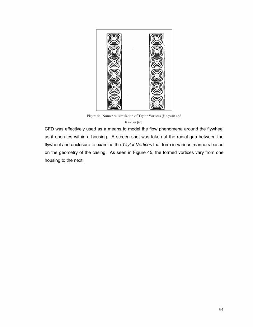
94

Figure 44. Numerical simulation of Taylor Vortices (He-yuan and

Kai-tai) [43].

CFD was effectively used as a means to model the flow phenomena around the flywheel

as it operates within a housing. A screen shot was taken at the radial gap between the

flywheel and enclosure to examine the Taylor Vortices that form in various manners based

on the geometry of the casing. As seen in Figure 45, the formed vortices vary from one

housing to the next.

95

C O N C L U S I O N S

A theoretical study was conducted in order to determine the feasibility of, and if possible,

the optimum design of a high inertia flywheel and casing to be implemented as a wind

energy storage system. A theoretical parasitic drag analysis was completed to determine

the viscous moment of the current flywheel when rotating within an enclosure. The

flywheel, when operating in free space, will experience a viscous moment range between

6,000 and 8,000 Newton-meters, depending on which theoretical method is employed.

Four different flow regimes were considered to help predict the flow pattern around the

flywheel, based on the geometry of the casing. Delineating the type of flow present in the

chamber is advantageous as a more specific coefficient equation can be utilized based on

the boundary layer interactions. An initial procedure was to determine the viscous torque

of the flywheel operating in unbound, free space (i.e., if operating on level ground at

atmospheric conditions). When placed in an enclosure, the moment coefficient for the

turbulent regime is effectively reduced from a range of [0.005-0.006] down to a range of

[0.0025-0.0035] (using various theoretical methods). The flywheel experiences a 15

percent decrease in drag by being placed within a tightly spaced enclosure. The optimal

spacing for the range of operation of the flywheel under investigation was found to be

0.0826 meters in the axial and radial directions (note: this is based on a specific list of

casing geometries modeled in FLUENT). When the chamber pressure around the

flywheel was reduced to the target of 120 of an atmosphere, the parasitic drag was

reduced an additional 75 percent, compared to the friction moment experienced while

revolving in free space.

The initial reduction in friction torque experienced when the flywheel operates in an

enclosure can be attributed to the existence of “core flow” when boundary layers remain

very close, but separated. This core has been found to rotate at approximately half the

angular velocity of the flywheel. The decrease in torque is most likely caused by a

reduction in the transverse gradient of the tangential velocity to approximately half of what

it would on a free disk. Radial velocity gradients are only present in the boundary layers

attached to the flywheel and enclosure. The space in between them lacks this radial

velocity, enabling the core to experience solid body rotation.

In closing, It is particularly noteworthy that, apart from the case of very small gaps

the moment of viscous forces is almost completely independent of the width of the gap, as

96

seen from the moment coefficient calculated. Comparing coefficients of free disk versus

housing, it is seen that the moment on a free disk is greater than that on a disk in a

housing. This fact can be explained by the existence of the core which moves at half the

angular velocity. This decreases the transverse gradient of the tangential velocity to

approximately one half of what it would be on a free disk and, consequently, the drag is

also smaller than on a free disk.

The resulting viscous moment calculated in FLUENT for the flywheel was

considerably lower than the theoretical solutions obtained. Further investigation of the

current flywheel needs to be completed within FLUENT. The flow characteristics around

the flywheel resembled expected results, as Taylor vortices formed in the radial gap as the

Reynolds number was increased. Also, the formation of boundary layers can be seen on

both the flywheel and housing walls, depending on the gap clearance.

97

F U T U R E W O R K / R E C O M M E N D A T I O N S

There are various aspects of this flywheel to study that can be improved

and/or changed in an attempt to amplify the results. The first recommendation is

to broaden this study by designing an experimental apparatus. A range of

theoretical values of parasitic drag of the flywheel were obtained. Thus, it is

necessary to design a scale model of the flywheel and enclosure combination to

get more specific results. Schultz-Grunow [31] and Daily and Nece [40] both

provide a detailed summary of the apparatus’ used in their respective studies.

Their techniques can be correlated to the flywheel and housing dimensions in an

attempt to obtain exact drag measurements for a flywheel operating in an

enclosure; to this point, no information exists of this manner, pertaining to flywheel

operation. This experimental design will need to have the capabilities to cover a

higher range of Reynolds numbers; the experimental data can then be used as a

means of comparison for the theoretically determined moment coefficients from

this study. Also of particular importance for the future experimental apparatus is

the ability to change the system’s geometry to further examine optimal gap

clearance. Thus, it is recommended that an interchangeable disk system with a

rigid cylindrical housing be designed so that disks of various diameters and

thicknesses can be tested.

Also, a more in depth CFD analysis is in order to use as a supplement to

the theoretical calculations contained in this thesis. Heat transfer (i.e., viscous

heating) is a major emphasis to include in future CFD work. If an excess of

heating occurs, a further means to cool the flywheel might need to be employed as

well. A three-dimensional model would also serve as a means to further verify the

current theoretical and numerical data included in this effort.

Finally, experimental data exists concerning surface roughness and

polymer solutions exists which could be beneficial. This data could be useful to

determine improved surfaces to be placed on the flywheel and enclosing walls

which could help further reduce parasitic drag. It must also be determined what

the machining capabilities are on an application such as this; more specifically,

98

what is the smallest possible gap obtained such that the enclosure can safely and

effectively be built around the flywheel.

99

R E F E R E N C E S

[1] Anderson, J.D., Jr., Fundamentals of Aerodynamics, 3rd ed., McGraw Hill, New York (2001). [2] Bertin, J.J., Aerodynamics for Engineers, 4th ed., Prentice Hall, Upper Saddle River, NJ (2002). [3] Young, D.F., B.R. Munson, and T.H. Okiishi, A Brief Introduction to Fluid Mechanics, 3rd ed., John Wiley & Sons, Inc., Hoboken, NJ (2004). [4] Schlichting, H., Boundary Layer Theory, 7th ed., McGraw Hill, New York (1979). [5] Batten, W.M.J., S.R. Turnock, N.W. Bressloff, and S.M. Abu-Sharkh, “Turbulent Taylor- Couette Vortex Flow Between Large Radius Ratio Concentric Cylinders,” Experiments in Fluids, 36, 419-421 (2004). [6] Anderson, J.D., Jr., “Ludwig Prandtl’s Boundary Layer,” American Institute of Physics, Physics Today, 42-48 (2005). [7] White, F.M., Viscous Fluid Flow, 3rd ed., McGraw Hill International Edition, Singapore (2006). [8] Nelka, J.J., “Evaluation of a Rotating Disk Apparatus: Drag of a Disk Rotating in a Viscous Fluid,” Department of the Navy, R & D Center: Ship Performance Department, Research and Development Report. Report 3851 (1973). [9] Anderson, J.D., Jr., Introduction to Flight, 4th ed., McGraw Hill, New York (2000). [10] Pai, Shih-I, Introduction to the Theory of Compressible Flow. D. VanNostrand Company, Inc., Princeton, NJ (1959). [11] Graebel, W.P., Advanced Fluid Mechanics, Academnic Press, New York (2007). [12] Tu, J., Yeoh, G.H., and C. Liu, Computational Fluid Dynamics: A Practical Approach. Butterworth-Heinermann, Burlington, MA (2008). [13] Miyazoe, Y., T. Sawairi, K. Ito, Y. Konishi, T. Yamane, M. Nishida, B. Asztalos, T. Masuzawa, T. Tsukiya, S. Endo, and Y. Taenaka, “Computational Fluid Dynamics Analysis to Establish the Design Process of A Centrifugal Blood Pump: Second Report,” ISAO, Artificial Organs, 23, No. 8, 762-768 (1999). [14] Anderson, J.D., Jr., Computational Fluid Dynamics: The Basics with Applications, McGraw Hill, New York (1995). [15] Hinko, K.A., “Transitions in the Small Gap Limit of Taylor-Couette Flow,” REU Summer Research Program Technical Paper. Ohio State University (2003). [16] Batten, W.M.J., S.R. Turnock, N.W. Bressloff, and S.M. Abu-Sharkh, “Turbulent Taylor-Couette vortex flow between large radius ratio concentric cylinders,” Experiments in Fluids, 36, 419-421 (2004). [17] Kempf, G., “Uber Reibungswiderstand Rotierender Scheiben,” Vortrage auf dem Gebeit der Hydro- und Aerodynamik, Innsbruck Congress (1922), Berlin, 168 (1924). [18] Nelka, J.J., “Evaluation of a Rotating Disk Apparatus: Drag of a Disk Rotating in a Viscous Fluid,” U.S. Naval Ship R & D Center, Ship Performance Department, Report 3851 (1973). [19] Theodorsen, T. and R. Regier, “Experiments on Drag of Revolving Disks, Cylinders, and Streamline Rods at High Speeds,” National Advisory Council for Aeronautics, Report 793, 4-6 (1945). [20] Taylor, G.I., “Stability of a Viscous Liquid Contained Between Two Rotating Cylinders,” Philos. Trans. R. Soc. London Ser. A, 223, 289-343 (1923). [21] Rayleigh, Lord, “On the Dynamics of Revolving Fluids,” Proc. R. Soc. London. Ser. A, 93, 148-154 (1916). [22] Harrison, W.J., Proc. Cambridge Philos. Soc., 455 (1921) [23] von Karman, T., “On Laminar and Turbulent Friction,” National Advisory Committee for Aeronautics, TM 1092, 1, No. 4, 20-30 (1921).

100

[24] Cochran, W.G., “The Flow Due to a Rotating Disk,” Proc. Cambridge Philos. Soc., 30, 365-375 (1934). [25] Cumptsy, N., Jet Propulsion; A simple guide to the aerodynamic and thermodynamic design and perforemance of jet engines, Cambridge University Press, Cambridge (2007). [26] Stokes, G.C, “On the theories of internal friction of fluids in motion,” Transactions of the Cambidge. Philosophical Society, 8, 287-305 (1845). [27] Mills, A.F., Basic Heat and Mass Transfer, 2nd ed. Prentice Hall, Upper Saddle River, NJ (1999). [28] Moran, M.J. and H.N. Shapiro, Fundamentals of Engineering Thermodynamics, 5th ed., John Wiley & Sons, Inc., Hoboken, NJ (2004). [29] Stuart, J.T., “On the non-linear mechanics of hydrodynamic stability,” Journal of Fluid Mechanics, 4, 1-21, Cambridge (1958). [30] Srinivasan, R., S. Jayanti, and A. Kannan, “Effect of Taylor Vortices on Mass Transfer from a Rotating Cylinder,” AIChE Journal, Fluid Mechanics and Transport Phenomena, 51, no. 11, (2005). [31] Schultz-Grunow, F., Der Reibungswiderstand rotierender Scheiben in Gehausen. ZAMM 15, 191- 204 (1935). [32] Stuart, J.T., and R.C. DiPrima, “On the mathematics of Taylor-vortex flows in cylinders of finite length,” Proceedings of the Royal Society of London, series A, 373, 357-365 (1980). [33] Meksyn, D. and J.T. Stuart,” Stability of viscous motion between parallel planes for finite disturbances,” Proceedings of the Royal Society of London, series A, 208, 517-526 (1951). [34] Sparrow, E.M., and J.L. Gregg, “Mass transfer, flow and heat transfer about a rotating disk,” Transactions ASME, Journal of Heat Transfer, 82, 294-302 (1960). [35] Goldstein, S., “On the resistance to the rotation of a disk immersed in a fluid,” Proceedings of the Cambridge Philosophical Society, 31, part 2, 232 (1935). [36] Goldstein, S., “The Similarity theory of Turbulence, and Flow between Parallel Planes and through Pipes,” Proceedings of the Royal Society of London, series A, 159, no. 899, 473-496 (1937). [37] Dorfman, L.A., “Effect of Radial Flow between the Rotating Disc and Housing on their Resistance and Heat Transfer,” [38] Dorfman, L.A., Hydrodynamic Resistance and the Heat Loss of Rotating Solids, Oliver and Boyd, 1st ed., 1-71 (1963). [39] Granville, P.S., “The Torque and Turbulent Boundary Layer of Rotating Disks with Smooth and

Rough Surfaces, and in Drag-Reducing Polymer Solutions,” Journal of Ship Research, 17, no. 4, 181-195 (1973).

[40] Daily, J.W. and R.E. Nece, “Chamber dimension effects on induced flow and friction resistance of enclosed rotating disks,” Journal of Basic Engineering, Trans. ASME, series D, 82, 217-232 (1960).

[41] Maleque, K.A. and M.A. Sattar, “Steady Laminar Flow with variable properties due to a porous rotating disk,” Trans. ASME, Journal of Heat Transfer, 127, 1406-1409 (2005).

[42] Celik, I.B., Introductory Numerical Methods for Engineering Applications, Ararat Books and Publishing, LCC, Morgantown (2001).

[43] He-yuan, W. and L. Kai-tai, “Spectral Galerkin Approximation of Couette-Taylor Flow,” Applied Mathematics and Mechanics, English Edition, 25, no. 10, 1184-1193 (2004).

[44] Srinivasan, R., S. Jayanti, and A. Kannan, “Effect of Taylor Vortices on Mass Transfer from a Rotating Cylinder,” AIChE Journal, Fluid Mechanics and Transport Phenomena, 51, no. 11, 2885-2898 (2005).

[45] Shigley, J.E., C.R. Mischke, and R.G. Budynas, Mechanical Engineering Design, 7th ed., McGrawHill, New York (2004).

[46] GAMBIT 2.3, Geometry Modeling and High Quality MeshingUser’s Guide. FLUENT, Inc. (2006).

[47] FLUENT User’s Guide, Version 6.2. ANSYS, Inc. (2005). [48] FLUENT User’s Guide, Version 6.3. ANSYS, Inc. (2006).

101

[49] Uyehara, O.A. and K.M Watson, “High Pressure Vapor-Liquid Equilibria,” Natl. Pet. News, 36, R623-RR635 (1944).

[50] Owczarek, J.A., Fundamentals of Gas Dynamics. International Textbook Company. Scranton, PA (1968).

[51] Cambel, A.B. and B.H. Jennings, Gas Dynamics. McGraw Hill Series in Mechanical Engineering. McGraw Hill, New York (1958).

[52] Hinko, K.A., “Transitions in the Small Gap Limit of Taylor-Couette Flow,” REU Summer Research Program Technical Paper. Ohio State University (2003).

[53] Celik, I.B., “Procedure for estimation and Reporting of Discretization Error in CFD Applications,” Journal of Fluids Engineering Editorial Policy Statement on the Control of Numerical Accuracy; ASME Journal of Fluids Engineering , (2005).

[54] Schmeiden, C., “Uber den Widerstand einer in einer Flussigkeit rotierenden Scheibe,” ZAMM, 8, 460-479 (1928).

[55] S.L. Soo, “Laminar Flow Over an enclosed Rotating Disk,” Trans. ASME, 80, 287-296 (1958). [56] A.T. Ippen, “Influence of Viscometry on Centrifugal-Pump Performance,” Trans. ASME, 68, 823-

848 (1946).

102

A P P E N D I X A : M A T L A B C O D E

This appendix contains a code written within the MATLAB systems tool box. The two codes are used to calculate the derivative of the circumferential velocity component with respect to the axis of rotation. This will be used in equation (2.1) to calculate shear stress

(dudz

τ μ= ). The circumferential velocity components are given by White [7]. In the

following code, the subscripts one and two denote the radius of the inner cylinder and the radius of the enclosing walls, respectively. This equation is applicable to small radial clearances between the flywheel and cylindrical housing walls ( innerinnerouter RRR <<− ). Moderate Gap %MATLAB Systems Tool Box: Differentiation of Velocity with respect to %Flywheel Radius %MODERATE Gap: Peripheral Velocity Component %r1 = inner cylinder radius (disk) %r2 = outer cylinder radius (Housing) %r = radius at any point between the disk and housing %w1 = angular velocity of inner cylinder syms r r1 r2 w1 %define peripheral velocity between disk and housing u_theta=r1*w1*(((r2/r)-(r/r2))/((r2/r1)-(r1/r2))); %take derivative of u_theta with respect or 'r' dudr=diff(u_theta,r) dudr = r1*w1*(-r2/r^2-1/r2)/(r2/r1-r1/r2) >> pretty (dudr) / r2 1 \ r1 w1 |- ---- - ----| | 2 r2 | \ r / --------------------- r2 r1 ---- - ---- r1 r2

103

Small Gap %MATLAB Systems Tool Box: Differentiation of Velocity with respect to %Flywheel Radius %SMALL Gap: Peripheral Velocity Component %r = radius at any point between the disk and housing %r1 = inner cylinder radius (disk) %r2 = outer cylinder radius (housing) %w1 = angular velocity of inner cylinder syms r r1 r2 w1 %defibe peripheral velocity between disk and housing u_theta=r1*w1*(1-((r-r1)/(r2-r1))); %take derivative of u_theta with respect or 'r' dudr=diff(u_theta,r) dudr = -r1*w1/(r2-r1) >> pretty (dudr) r1 w1 - ------- r2 - r1

104

A P P E N D I X B : M O M E N T C O E F F I C I E N T S U M M A R Y T A B L E S

This appendix offers a summary of the moment coefficients discussed and utilized in this study. The tables offer credit to the deserved party, the applicable flow regime, and the section of the disk the coefficient is concerned; the term ‘disk’ refers to the circular top and bottom faces of the flywheel.

Table B1. Theoretical Moment Coefficient Summary of Past Researchers (disk faces)

Researcher Flow Regime Moment Coefficient Surroundings/

Area

von Kármán Laminar 1 2

3.68M

e

CR

= unbound disk (both sides)

von Kármán Turbulent 51146.0

eM R

C = unbound disk (both sides)

Cochran Laminar 21

87.3

eM R

C = unbound disk (both sides)

Cochran Laminar (v. Karman Correction) 21

38.3

eM R

C =

unbound disk (both sides)

Goldstein Turbulent ( ) 3.0log97.11+= Me

M

CRC

unbound disk (both sides)

Granville Turbulent (agrees w/ Cochran) 1 2

3.87M

e

CR

= unbound disk (both sides)

Granville Laminar

& Turbulent

( ) ( ) ( )5 2

2 tr

tr tr

eM M M Mturb turb lam

e

RC C C C

R⎛ ⎞ ⎡ ⎤= − −⎜ ⎟ ⎣ ⎦⎝ ⎠

unbound disk (both sides)

Dorfman Turbulent 58.2)(log982.0 −= eM RC unbound disk (both sides)

Schultz-Grunow Laminar 21

67.2

eM R

C = enclosed disk (both sides)

Schultz-Grunow Turbulent 51

0622.0

eM R

C = enclosed disk (both sides)

Schlicthing Laminar 12M

e

RCs R

π= enclosed disk (both sides)

Ippen Laminar 1 2

2.600M

e

CR

= enclosed disk (both sides)

Ippen Turbulent 1 5

0.0836M

e

CR

= enclosed disk (both sides)

105

Table B2. Theoretical Moment Coefficient Summary of Past Researchers (disk edge) Researcher Flow Regime Moment Coefficient Surroundings/Area

Schlichting Laminar 12M

e

RCs R

π′ = enclosed disk/edge

Schmieden Laminar Me

KCR

′ = where 2K R sπ= enclosed disk/edge

Dorfman Laminar ( )( )1 2.5M MhC C R

′ = + unbound or enclosed

disk/edge

Daily/Nece Laminar ωνπ

cabCM 2

4=′ enclosed disk/edge

Daily/Nece Turbulent abfCM 8

π=′ enclosed disk/edge

Daily/Nece Laminar ( ) e

M RasC π2

= enclosed disk/ faces and edge

Daily/Nece Laminar

( )21

10170.3

eM R

asC = enclosed disk/ faces and edge

Daily/Nece Turbulent ( ) 4161

080.0

eM Ras

C = enclosed disk/ faces and edge

Daily/Nece Turbulent ( )

51

1010102.0

eM R

asC = enclosed disk/ faces and edge

106

A P P E N D I X C : M O O D Y D I A G R A M

This appendix includes the Moody diagram to determine the friction factor of a pipe ( f ). This factor is used to determine the moment coefficient for the edge of a rotating disk within a housing; from the experiments of Daily and Nece. The friction factor, f , is used in equation (2.57) of this report. The roughness coefficient, K, will be estimated to compare to commercial steel (K= 0.046).

Figure C1. Moody Diagram [45].

107

A P P E N D I X D : C F D D A T A T A B L E S

This appendix includes the data collected from CFD simulations from FLUENT. The main purpose of the provided data tables is to prove both grid independence and iterative convergence.

Table 11. Housing 3: Impact of Flywheel Edge on Total Moment (FLUENT) Continuity Adapt Cells Faces Nodes MTotal CGI MTop MBottom Medge MTop/Bottom/MTotal MEdge/MTotal

--- --- --- --- --- N-m % N-m N-m N-m --- ------ 18750 38275 19526 -813.91 --- -242.41 -242.41 -329.10 0.60 0.401 37098 76505 39408 -751.12 7.71 -227.21 -227.21 -296.71 0.60 0.402 79346 168202 89562 -722.23 3.85 -216.21 -216.21 -289.82 0.60 0.403 136543 279043 140289 -721.98 0.03 -208.21 -208.21 -305.57 0.58 0.423 136543 279043 140289 -721.98 0.00 -208.21 -208.21 -305.57 0.58 0.42

1x10-4 3 136543 279043 140289 -721.98 0.00 -208.21 -208.21 -305.57 0.58 0.42

1x10-3

Table 12. Housing 4: Impact of Flywheel Edge on Total Moment (FLUENT) Continuity Adapt Cells Faces Nodes MTotal CGI MTop MBottom Medge MTop/Bottom/MTotal MEdge/MTotal

--- --- --- --- --- N-m % N-m N-m N-m --- ------ 57600 116225 58626 -853.88 --- -309.84 -309.84 -234.20 0.73 0.271 80850 164630 83781 -801.68 6.11 -293.18 -293.18 -215.32 0.73 0.272 129798 266610 136813 -781.20 2.55 -272.71 -272.71 -235.78 0.70 0.303 323400 652660 329261 -779.12 0.27 -271.18 -271.18 -236.76 0.70 0.303 323400 652660 329261 -798.73 2.52 -269.26 -269.26 -260.21 0.67 0.33

1x10-4 3 323400 652660 329261 -797.29 0.18 -272.36 -272.24 -252.69 0.68 0.32

1x10-3

Table 13. Housing 5: Impact of Flywheel Edge on Total Moment (FLUENT)

Continuity Adapt Cells Faces Nodes MTotal CGI MTop MBottom Medge MTop/Bottom/MTotal MEdge/MTotal

--- --- --- --- --- N-m % N-m N-m N-m --- ------ 11760 24748 12989 -1420.27 --- -411.23 -411.23 -597.81 0.58 0.421 40980 85428 44449 -1228.95 13.47 -338.43 -338.43 -552.09 0.55 0.452 114270 236900 122631 -1065.33 13.31 -302.39 -302.39 -460.55 0.57 0.433 163920 334776 170857 -1066.36 0.10 -301.93 -303.88 -460.55 0.57 0.433 163920 334776 170857 -1070.69 0.41 -305.01 -303.05 -462.63 0.57 0.43

1x10-4 3 163920 334776 170857 -1067.77 0.27 -304.89 -302.91 -459.97 0.57 0.43

1x10-3

Table 14. Housing 6: Impact of Flywheel Edge on Total Moment (FLUENT)

Continuity Adapt Cells Faces Nodes MTotal CGI MTop MBottom Medge MTop/Bottom/MTotal MEdge/MTotal

--- --- --- --- --- N-m % N-m N-m N-m --- ------ 10752 22456 11705 -1377.76 --- -448.31 -448.31 -481.14 0.65 0.351 33348 69416 36069 -1232.41 10.55 -395.90 -395.90 -440.61 0.64 0.362 78792 164096 85305 -1112.32 9.74 -345.37 -345.37 -421.58 0.62 0.383 133392 272224 138833 -1116.13 0.34 -346.69 -345.81 -423.63 0.62 0.383 133392 272224 138833 -1119.24 0.28 -344.61 -345.50 -429.13 0.62 0.38

1x10-4 3 133392 272224 138833 -1119.30 0.01 -344.61 -345.50 -429.19 0.62 0.38

1x10-3