PARAMETERS IDENTIFICATION OF A POWER PLANT MODEL FOR THE SIMULATION … · Parameters...
14
U.P.B. Sci. Bull., Series C, Vol. 72, Iss. 1, 2010 ISSN 1454-234x PARAMETERS IDENTIFICATION OF A POWER PLANT MODEL FOR THE SIMULATION OF ISLANDING TRANSIENTS Alberto BORGHETTI 1 , Mauro BOSETTI 2 , Carlo ALBERTO NUCCI 3 , Mario PAOLONE 4 The paper presents a procedure for parameter identification along with its application to the model of a combined cycle power plant that includes the surrounding electrical network, built for the analysis of islanding maneuvers transients. The paper illustrates both the power system computer model, implemented within the EMTP-RV simulation environment, and the developed identification procedure based on the interface between the developed model and Matlab. The parameter identification procedure is applied to experimental transient recordings that make reference to a similar power plant. Keywords: power plant, parameter identification, islanding, electromechanical transients 1. Introduction The complexity of power plants operation, of their interaction with the electrical network, as well as the need of implementing coordinated control systems to cope with specific operational requirements, call for the development/use of advanced and accurate simulation tools. This may represent the adequate complement or substitute the practice of repetitive prototyping and expensive tests on real systems. Within this context, the parameter identification of power plant dynamic models represents one of the main issues for proper simulation of the transients occurring during critical operation conditions [1-3] *) . This paper deals with a parameter-identification procedure conceived for the development of a computer simulator aimed at reproducing the islanding and black-startup energization transients of a power system consisting of a combined 1 Prof., Department of Electrical Engineering, University of Bologna, Italy 2 Prof., Department of Electrical Engineering, University of Bologna, Italy 3 Prof., Department of Electrical Engineering, University of Bologna, Italy 4 Prof., Department of Electrical Engineering, University of Bologna, Italy *) The contents of the paper are based on a previous work presented at by the Authors at the 9th International Conference on Modeling and Simulation of Electric Machines, Converters and Systems (Electrimacs 2008), June 8-11, 2008, Québec city, Canada.
Transcript of PARAMETERS IDENTIFICATION OF A POWER PLANT MODEL FOR THE SIMULATION … · Parameters...

U.P.B. Sci. Bull., Series C, Vol. 72, Iss. 1, 2010 ISSN 1454-234x
PARAMETERS IDENTIFICATION OF A POWER PLANT MODEL FOR THE SIMULATION OF ISLANDING
TRANSIENTS
Alberto BORGHETTI1, Mauro BOSETTI2, Carlo ALBERTO NUCCI3, Mario PAOLONE4
The paper presents a procedure for parameter identification along with its application to the model of a combined cycle power plant that includes the surrounding electrical network, built for the analysis of islanding maneuvers transients. The paper illustrates both the power system computer model, implemented within the EMTP-RV simulation environment, and the developed identification procedure based on the interface between the developed model and Matlab. The parameter identification procedure is applied to experimental transient recordings that make reference to a similar power plant.
Keywords: power plant, parameter identification, islanding, electromechanical transients
1. Introduction
The complexity of power plants operation, of their interaction with the electrical network, as well as the need of implementing coordinated control systems to cope with specific operational requirements, call for the development/use of advanced and accurate simulation tools. This may represent the adequate complement or substitute the practice of repetitive prototyping and expensive tests on real systems.
Within this context, the parameter identification of power plant dynamic models represents one of the main issues for proper simulation of the transients occurring during critical operation conditions [1-3]*).
This paper deals with a parameter-identification procedure conceived for the development of a computer simulator aimed at reproducing the islanding and black-startup energization transients of a power system consisting of a combined
1 Prof., Department of Electrical Engineering, University of Bologna, Italy 2 Prof., Department of Electrical Engineering, University of Bologna, Italy 3 Prof., Department of Electrical Engineering, University of Bologna, Italy 4 Prof., Department of Electrical Engineering, University of Bologna, Italy *) The contents of the paper are based on a previous work presented at by the Authors at the 9th International Conference on Modeling and Simulation of Electric Machines, Converters and Systems (Electrimacs 2008), June 8-11, 2008, Québec city, Canada.

102 Alberto Borghetti, Mauro Bosetti, Carlo Alberto Nucci, Mario Paolone
cycle power plant (CCPP), the local distribution network and relevant loads, (see Fig. 1).
In particular, the computer simulator refers to a 80 MW power plant composed by two aero-derivative gas turbine (GT) units and a steam turbine unit (ST) in combined cycle. The simulator represents the dynamic behavior of the GTs, the heat recovery steam generator (HRSG), the ST and their control systems [4-8]. Concerning the electrical apparatus, it includes the model of the synchronous generators along with their exciters, automatic voltage regulators (AVRs) [9-10], as well as the representation of the local electrical network (step-up unit transformers, cable link between power plant substation and distribution substation and loads) connected to the external transmission network.
All the models are implemented in the EMTP-RV simulation environment ([11-13]) and are aimed at representing both transients following energization process, typically after a blackout condition, and transients due to islanding maneuvers that disconnect the CCPP and the local network from the external transmission network.
800
m c
able
line
External transmission network
cabl
e lin
e
External transmission network
GT1 GT2 Fig.1. Scheme of the considered CCPP and the surrounding electrical network
The applied parameter identification procedure is based on an interface
between the EMTP-RV and Matlab that has been developed to implement a non-linear data fitting algorithm. The parameter identification procedure makes use of available test recordings.
Parameters identification of a power plant model for the simulation of islanding transients 103
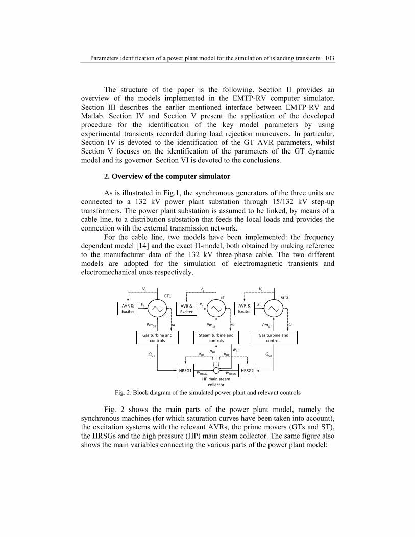
The structure of the paper is the following. Section II provides an overview of the models implemented in the EMTP-RV computer simulator. Section III describes the earlier mentioned interface between EMTP-RV and Matlab. Section IV and Section V present the application of the developed procedure for the identification of the key model parameters by using experimental transients recorded during load rejection maneuvers. In particular, Section IV is devoted to the identification of the GT AVR parameters, whilst Section V focuses on the identification of the parameters of the GT dynamic model and its governor. Section VI is devoted to the conclusions.
2. Overview of the computer simulator
As is illustrated in Fig.1, the synchronous generators of the three units are connected to a 132 kV power plant substation through 15/132 kV step-up transformers. The power plant substation is assumed to be linked, by means of a cable line, to a distribution substation that feeds the local loads and provides the connection with the external transmission network.
For the cable line, two models have been implemented: the frequency dependent model [14] and the exact Π-model, both obtained by making reference to the manufacturer data of the 132 kV three-phase cable. The two different models are adopted for the simulation of electromagnetic transients and electromechanical ones respectively.
AVR & Exciter
Gas turbine and controls
HRSG1 HRSG2
Steam turbine and controls
Gas turbine and controls
PmGT PmST PmGT
QGT
HP main steam collector
wHRSG
wST
GT1 ST GT2
QGT
ω ω ω
pHP
wHRSG
Ef
Vt
AVR & Exciter
Ef AVR & Exciter
Ef
VtVt
pHPpHP
Fig. 2. Block diagram of the simulated power plant and relevant controls
Fig. 2 shows the main parts of the power plant model, namely the
synchronous machines (for which saturation curves have been taken into account), the excitation systems with the relevant AVRs, the prime movers (GTs and ST), the HRSGs and the high pressure (HP) main steam collector. The same figure also shows the main variables connecting the various parts of the power plant model:

104 Alberto Borghetti, Mauro Bosetti, Carlo Alberto Nucci, Mario Paolone
Vt terminal voltage of the synchronous generators Ef field voltage ω angular speed of the generators rotors PmGT mechanical output power of a GT PmST mechanical output power of the ST QGT thermal power provided by the GT exhaust gas wHRSG output steam mass flow rate of a HRSG wST inlet steam mass flow to the ST pHP pressure in the HP main steam collector. The initial states of the GTs models, the excitation systems and the AVRs
models are defined by the results of the initial network power flow calculation. The states of the HRSGs and the states of the ST model are initialized from the initial values of QGT1, QGT2 and those of wHRSG1, wHRSG2 respectively, assuming pressure pHP be equal to the rated value and that the by-pass valves be closed.
Each of the three synchronous generators has two inputs: excitation voltage Ef and mechanical power Pm.
The excitation voltages are provided by the AVR and brushless exciter models of the GT units and ST unit. The model of GT AVR and exciter corresponds to the AC8B Type of the IEEE Std. 421. [9]. The GT AVR parameter values are identified from available load rejection transient record, as described in Section IV. The ST AVR is based on a simple PI regulator with a lead-lag compensator.
The mechanical power values are provided by the models of the GTs (PmGT) and the one of the ST (PmST).
Table 1 Values of the synchronous machines electrical parameters
xd x'd x”d xq x’q T’d T”d T’q x0 xl GT 2.13 0.29 0.18 1.09 0.43 1.09 0.04 0.04 0.13 0.13 ST 2.2 0.29 0.2 1.11 0.4 1.3 0.08 0.075 0.07 0.15
The model adopted for the two GTs is based on a transfer function that
represents the dynamic link between fuel flow rate and output mechanical power and includes the fuel metering valve (FMV) dynamic and a speed governor. Section V is devoted to the parameter identification of the GT model and of its speed governor, together with the parameter identification of a two-mass model of the GT train drive.
The HRSG model is adapted from the one proposed in [5], relevant to the HP section with a bypass control valve at the HRSG output. The model is based on the following main assumptions: fast feed water adjustments, negligible effects of temperature control and water flows to the attemperators, constant enthalpy value of the steam at the ST inlet.

Parameters identification of a power plant model for the simulation of islanding transients 105
As shown in Fig. 2 and Fig. 2, the inputs of the HRSG model are QGT and pHP. QGT is assumed to be a non-linear function of the gas turbine output power PmGT [4]. Concerning pHP, it is calculated from the difference between the steam mass flow rate at the HRSGs outputs (wHRSG) and the steam turbine inlet mass flow rate (wST) through a transfer function that takes into account the time constant associated with the steam storage capacity into the collector volume.
‐QGT +
1/sTe
Ksh 1/sTsh
+
‐
By‐pass valve
‐
+
+ +
Ke
+
pHP
‐
wHRSGwe
wsh
psh
peEvaporator and
drum
SH(steam
equivalent)
Fig. 3. Model of the HRSG
Fig. 3 illustrates the structure of the implemented HP section HRSG
model, which takes into account the evaporator time constant Te for the calculation of the pressure pe in the drum according to the energy balance equation, a time constant Tsh relevant to the superheaters (SH) storage capacity. The steam flow rates between drum and SH and between SH and the collector are determined from the pressure drop relationship with flow rate being proportional to square root of pressure drop.
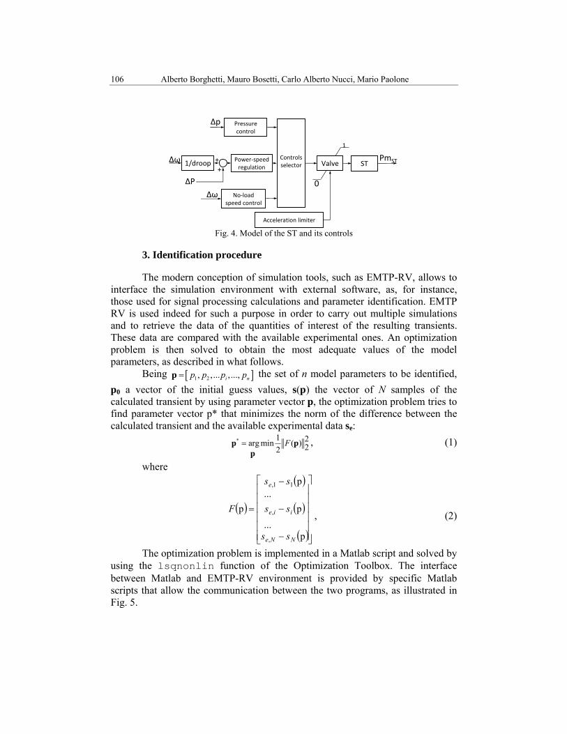
The model of the steam turbine, shown in Fig. 4, represents the time delay associated with the steam store in the inlet chest, the main valve dynamic implements three control operation modes: i) no-load speed control, ii) control to keep a constant value of upstream pressure pHP, iii) power and speed regulation. The no-load speed control mode is used at the startup and synchronizing phases, whilst in normal conditions the two modes are the pressure control or power-speed regulation.
106 Alberto Borghetti, Mauro Bosetti, Carlo Alberto Nucci, Mario Paolone
No‐loadspeed control
∆ω
Power‐speedregulation
∆ω++
∆P
1/droopControlsselector Valve
1
0
ST PmST
Acceleration limiter
Pressurecontrol
∆p
Fig. 4. Model of the ST and its controls
3. Identification procedure
The modern conception of simulation tools, such as EMTP-RV, allows to interface the simulation environment with external software, as, for instance, those used for signal processing calculations and parameter identification. EMTP RV is used indeed for such a purpose in order to carry out multiple simulations and to retrieve the data of the quantities of interest of the resulting transients. These data are compared with the available experimental ones. An optimization problem is then solved to obtain the most adequate values of the model parameters, as described in what follows.
Being [ ]1 2, ,... ,...,i np p p p=p the set of n model parameters to be identified, p0 a vector of the initial guess values, s(p) the vector of N samples of the calculated transient by using parameter vector p, the optimization problem tries to find parameter vector p* that minimizes the norm of the difference between the calculated transient and the available experimental data se: * 1 2arg min ( ) 22
F=p pp
, (1)
where
( )
( )
( )
( )⎥⎥⎥⎥⎥⎥
⎦
⎤
⎢⎢⎢⎢⎢⎢
⎣
⎡
−
−
−
=
p...
p...
p
p
,
,
11,
NNe
iie
e
ss
ss
ss
F, (2)
The optimization problem is implemented in a Matlab script and solved by using the lsqnonlin function of the Optimization Toolbox. The interface between Matlab and EMTP-RV environment is provided by specific Matlab scripts that allow the communication between the two programs, as illustrated in Fig. 5.
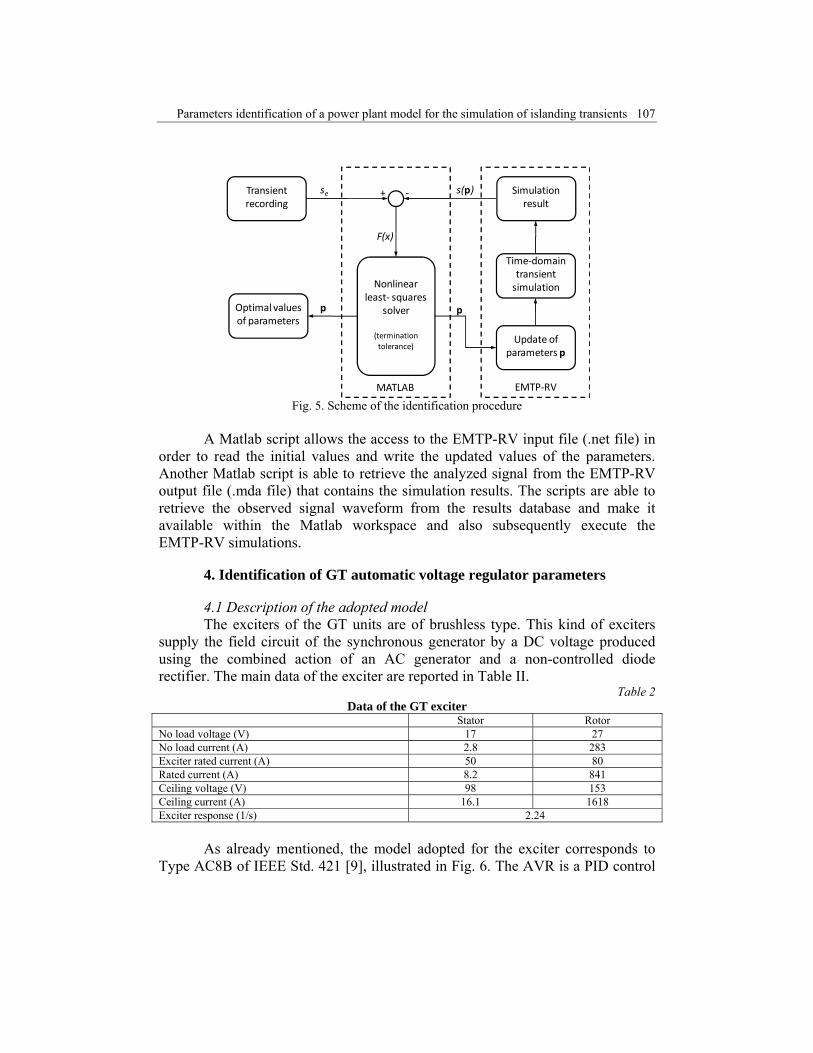
Parameters identification of a power plant model for the simulation of islanding transients 107
MATLAB
Nonlinear least‐ squares
solver
(termination tolerance)
F(x)
p
Update of parameters p
Time‐domain transient simulation
Transientrecording
Optimal values of parameters
Simulation result
s(p)se
EMTP‐RV
p
+ ‐
Fig. 5. Scheme of the identification procedure
A Matlab script allows the access to the EMTP-RV input file (.net file) in
order to read the initial values and write the updated values of the parameters. Another Matlab script is able to retrieve the analyzed signal from the EMTP-RV output file (.mda file) that contains the simulation results. The scripts are able to retrieve the observed signal waveform from the results database and make it available within the Matlab workspace and also subsequently execute the EMTP-RV simulations.
4. Identification of GT automatic voltage regulator parameters
4.1 Description of the adopted model The exciters of the GT units are of brushless type. This kind of exciters
supply the field circuit of the synchronous generator by a DC voltage produced using the combined action of an AC generator and a non-controlled diode rectifier. The main data of the exciter are reported in Table II.
Table 2 Data of the GT exciter
Stator Rotor No load voltage (V) 17 27 No load current (A) 2.8 283 Exciter rated current (A) 50 80 Rated current (A) 8.2 841 Ceiling voltage (V) 98 153 Ceiling current (A) 16.1 1618 Exciter response (1/s) 2.24
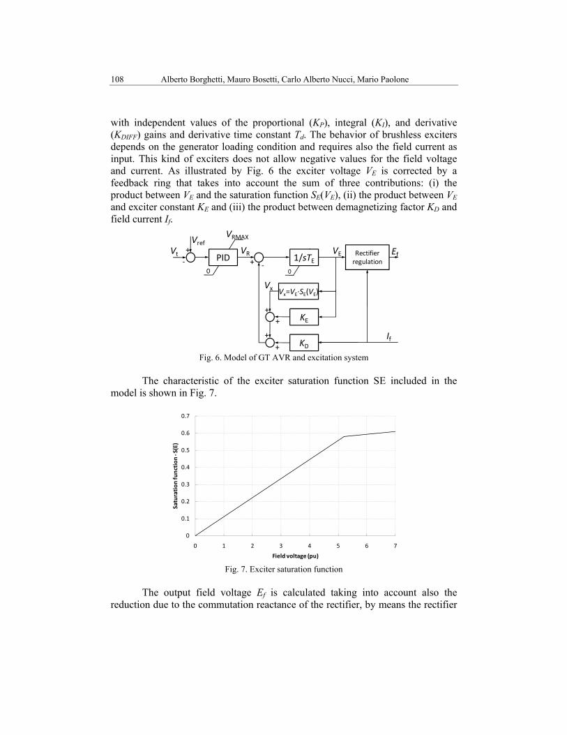
As already mentioned, the model adopted for the exciter corresponds to
Type AC8B of IEEE Std. 421 [9], illustrated in Fig. 6. The AVR is a PID control
108 Alberto Borghetti, Mauro Bosetti, Carlo Alberto Nucci, Mario Paolone
with independent values of the proportional (KP), integral (KI), and derivative (KDIFF) gains and derivative time constant Td. The behavior of brushless exciters depends on the generator loading condition and requires also the field current as input. This kind of exciters does not allow negative values for the field voltage and current. As illustrated by Fig. 6 the exciter voltage VE is corrected by a feedback ring that takes into account the sum of three contributions: (i) the product between VE and the saturation function SE(VE), (ii) the product between VE and exciter constant KE and (iii) the product between demagnetizing factor KD and field current If.
+‐ + ‐
Rectifierregulation
Ef
Vx=VE∙SE(VE)
KE
KDIf
VEPID 1/sTEVR
VRMAX
0 0
Vt
Vref
++
++
Vx
Fig. 6. Model of GT AVR and excitation system
The characteristic of the exciter saturation function SE included in the
model is shown in Fig. 7.
0
0.1
0.2
0.3
0.4
0.5
0.6
0.7
0 1 2 3 4 5 6 7
Saturation
function
‐S(E)
Field voltage (pu)
Fig. 7. Exciter saturation function The output field voltage Ef is calculated taking into account also the
reduction due to the commutation reactance of the rectifier, by means the rectifier
Parameters identification of a power plant model for the simulation of islanding transients 109
regulation block. As explained in [9], the impedance of the AC source supplying the AC side of rectifiers is characterized by predominantly inductive impedance. The impedance causes a strongly non linear decrease of the rectifier voltage output. This effect depends on the value of the current supplied by the rectifier and is represented by means a rectifier loading factor Kc proportional to commutating reactance and the rectifier regulation characteristic.
The values of the main parameters adopted for the exciter model are reported in Table III.
Table 3 – Values of the main parameters of the GT exciter model
VRMAX = 11.9 KC = 0.29 KD = 1.03 KE = 1.0 TE = 0.31 E1 = 5.2 p.u.
E2 = 7 p.u. SE(E1) = 0.58 SE(E2) = 0.61
4.2. Identification results
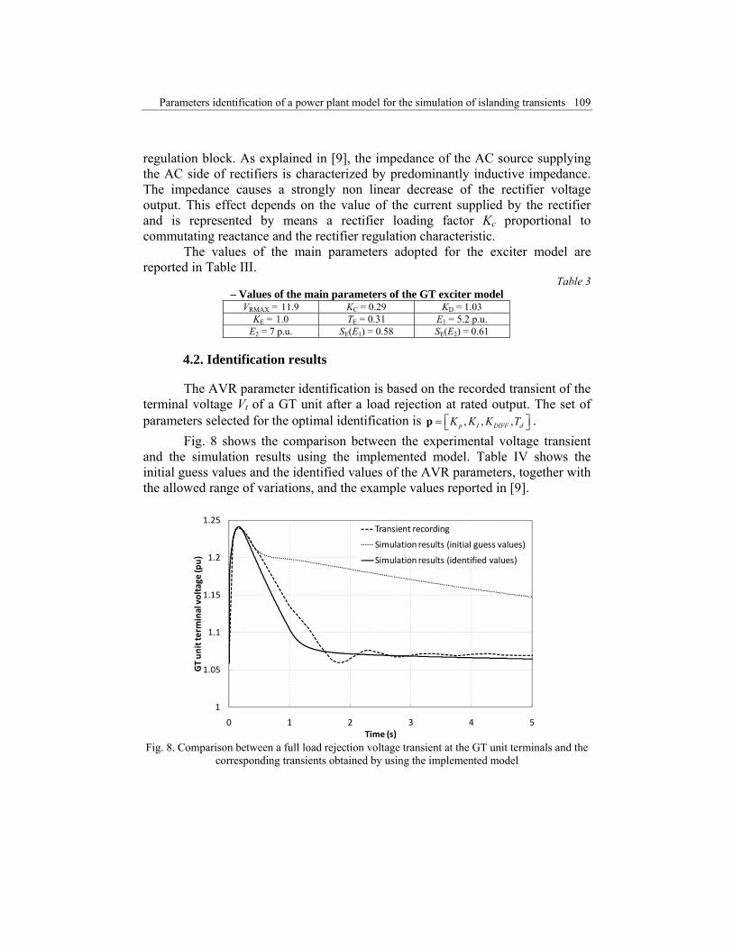
The AVR parameter identification is based on the recorded transient of the terminal voltage Vt of a GT unit after a load rejection at rated output. The set of parameters selected for the optimal identification is , , ,p I DIFF dK K K T⎡ ⎤= ⎣ ⎦p .
Fig. 8 shows the comparison between the experimental voltage transient and the simulation results using the implemented model. Table IV shows the initial guess values and the identified values of the AVR parameters, together with the allowed range of variations, and the example values reported in [9].
1
1.05
1.1
1.15
1.2
1.25
0 1 2 3 4 5
GT un
it te
rminal voltage
(pu)
Time (s)
Transient recording
Simulation results (initial guess values)
Simulation results (identified values)
Fig. 8. Comparison between a full load rejection voltage transient at the GT unit terminals and the
corresponding transients obtained by using the implemented model

110 Alberto Borghetti, Mauro Bosetti, Carlo Alberto Nucci, Mario Paolone
Table 4 Initial and identified AVR parameters, together with the allowed range of variations and the
example values reported in [9] Parameter Initial guess values Std. IEEE example
values Range Identified values
KP 35 80 7-280 132.8 KI 5 5 1-100 35.05
KDIFF 6 10 1-80 25.58 Td 0.1 0.1 - 0.012 5. Identification of the parameters of the GT dynamic model and its
governor
5.1. Description of the adopted model
The considered GT is an aeroderivative industrial RB211 package, characterized by a rated output to the electrical generator equal to 33 MW at 4850 rpm speed and by 94 kg/s exhaust mass flow at 503 °C.
The adopted model is illustrated in Fig. 9. As already mentioned the GT dynamics is represented by 4 poles-4 zeros transfer function that represent the dynamic link between fuel flow rate and output mechanical power
2
z31 z32z1 z2GT 2
p1 p2 p31 p32
( 1)( 1) ( 1)( )( 1) ( 1) ( 1)
s ss sGT s Ks s s s
τ ττ ττ τ τ τ
+ ++ += ⋅ ⋅
+ + + + , (3)
A feedback algebraic look-up table block determines the required
correction at partial loads. The FMV dynamic is represented by a first order transfer function with
time constant TFMV equal to 0.1 s. The droop of the speed governor is assumed equal to 5%. The model
includes also an acceleration limiter.
+
‐
PI
MAX
0
FMV π GTPm
Correction
PREF+
∆ω ω∙ω∙
0
+++
∆P
∆ω1/droop
Fig. 9. Model of the GT and its speed governor
Parameters identification of a power plant model for the simulation of islanding transients 111
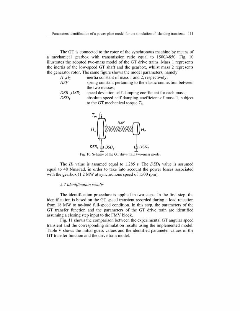
The GT is connected to the rotor of the synchronous machine by means of a mechanical gearbox with transmission ratio equal to 1500/4850. Fig. 10 illustrates the adopted two-mass model of the GT drive trains. Mass 1 represents the inertia of the low-speed GT shaft and the gearbox, whilst mass 2 represents the generator rotor. The same figure shows the model parameters, namely
H1,H2 inertia constant of mass 1 and 2, respectively; HSP spring constant pertaining to the elastic connection between
the two masses; DSR1,DSR2 speed deviation self-damping coefficient for each mass; DSD1 absolute speed self-damping coefficient of mass 1, subject
to the GT mechanical torque Tm.
TmHSP
H2H1
DSR1 DSR2DSD1
Fig. 10. Scheme of the GT drive train two-mass model The H2 value is assumed equal to 1.285 s. The DSD1 value is assumed
equal to 48 Nms/rad, in order to take into account the power losses associated with the gearbox (1.2 MW at synchronous speed of 1500 rpm).
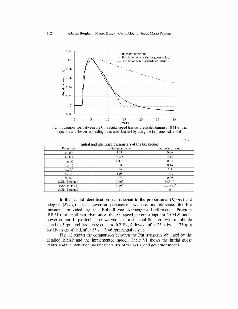
5.2 Identification results The identification procedure is applied in two steps. In the first step, the
identification is based on the GT speed transient recorded during a load rejection from 18 MW to no-load full-speed condition. In this step, the parameters of the GT transfer function and the parameters of the GT drive train are identified assuming a closing step input to the FMV block.
Fig. 11 shows the comparison between the experimental GT angular speed transient and the corresponding simulation results using the implemented model. Table V shows the initial guess values and the identified parameter values of the GT transfer function and the drive train model.
112 Alberto Borghetti, Mauro Bosetti, Carlo Alberto Nucci, Mario Paolone
0.98
1
1.02
1.04
1.06
1.08
1.1
1.12
0 5 10 15 20 25 30
Ang
ular sp
eed (p
u)
Time (s)
Transient recordingSimulation results (initial guess values)Simulation results (identified values)
Fig. 11. Comparison between the GT angular speed transient recorded during a 18 MW load
rejection and the corresponding transients obtained by using the implemented model
Table 5 Initial and identified parameters of the GT model
Parameter Initial guess value Optimized values τz2 (s) 3.13 0.06 τp2 (s) 30.03 5.15 τz31 (s) 0.032 0.24 τz32 (s) 0.31 0.16 τp31 (s) 0.38 0.3 τp32 (s) 1.08 1.08 H1 (s) 0.73 0.89
DSR1 (Nms/rad) 5 103 3.67 103 HSP (Nm/rad) 4 106 7.858 106
DSR2 (Nms/rad) 0 0 In the second identification step relevant to the proportional (KgovP) and
integral (KgovI) speed governor parameters, we use, as reference, the Pm transients provided by the Rolls-Royce Aeroengine Performance Program (RRAP) for small perturbations of the Δω speed governor input at 20 MW initial power output. In particular the Δω varies as a sinusoid function, with amplitude equal to 5 rpm and frequency equal to 0.2 Hz, followed, after 25 s, by a 1.73 rpm positive step of and, after 85 s, a 3.46 rpm negative step.
Fig. 12 shows the comparison between the Pm transients obtained by the detailed RRAP and the implemented model. Table VI shows the initial guess values and the identified parameter values of the GT speed governor model.

Parameters identification of a power plant model for the simulation of islanding transients 113
19.2
19.4
19.6
19.8
20
20.2
20.4
20.6
0 50 100 150 200 250
Mecha
nical pow
er (M
W)
Time (s)
Simulated transient referenceSimulation results (initial guess values)Simulation results(identified values)
Fig. 12. Comparison between the GT Pm transient simulated with a detailed model (reference) and
those obtained by the implemented model, for small speed perturbations
Table 6 Initial and identified parameters of the GT speed governor model
Parameter Initial guess value Identified values KgovP 7.5 2.1 KgovI 0.25 0.23
6. Conclusions
The paper has proposed ad identification procedure based on the coordinated use of a run-control interface between EMTP-RV and Matlab. The structure of the interface makes available the optimization tools of Matlab that have been used within the identification procedure.
The developed interface has been effectively applied for the parameter identification of a CCPP model aimed at simulating transients following energization process and transients due to islanding maneuvers.
The identified model appears a useful tool for the definition of both operational strategies and specific control systems in order to improve the probability of success of islanding maneuvers taking into account the various CCPP initial operating conditions.

114 Alberto Borghetti, Mauro Bosetti, Carlo Alberto Nucci, Mario Paolone
R E F E R E N C E S
[1]. J. L. Sancha, M. L. Llorens, J. M. Moreno, B. Meyer, J. F. Vernotte, W. W. Price, J. J. Sanchez-Gasca, “Application of long term simulation programs for analysis of system islanding,” IEEE Transactions on Power Systems, vol. 12, no. 1, pp. 189–197, Feb. 1997
[2]. CIGRE TF38.02.14, “Analysis and modeling needs of power systems under major frequency disturbances,” Rep., CIGRE Brochure no. 148, 1999
[3]. A. Borghetti, G. Migliavacca, C.A. Nucci, S. Spelta, “Black-start-up simulation of a repowered thermoelectric unit”, Control Engineering Practice, Vol. 9, pp. 791–803, 2001.
[4]. Cigre Task Force C4.02.25, Modeling of Gas Turbines and Steam Turbines in Combined Cycle Power Plants, 2003
[5]. K. Kunitomi, A. Kurita, Y. Tada, S. Ihara, W.W. Price, L.M. Richardson, G. Smith, “Modeling Combined-Cycle Power Plant for Simulation of Frequency Excursions”, IEEE Transactions on Power Systems, Vol. 18, No. 2, pp. 724-729, May 2003
[6]. S. Kiat Yee, J.V. Milanovic´, F.M. Hughes, “Overview and Comparative Analysis of Gas Turbine Models for System Stability Studies”, IEEE Transactions on Power Systems, Vol. 23, No. 1, pp. 108-118, Feb. 2008
[7]. M. E. Flynn, M. J. O’Malley, “A drum boiler model for long term power system dynamic simulation,” IEEE Transactions on Power Systems, vol. 14, no. 1, pp. 209–217, Feb. 1999
[8]. A.E. Nielsen, C. W. Moll, S. Staudacher, “Modeling and Validation of the Thermal Effects on Gas Turbine Transients”, Transactions of the ASME, Vol. 127, pp. 564-572, July 2005
[9]. IEEE Std 421.5™-2005 - IEEE Recommended Practice for Excitation System Models for Power System Stability Studies
[10]. P. Kundur, P. L. Dandeno, “Implementation of Synchronous Machine Models into Power System Stability Programs,” IEEE Transactions on Power Apparatus and Systems, vol. PAS-102, pp. 2047–2054, July 1983
[11]. J. Mahseredjian, S. Lefebvre, X.-D. Do, “A new method for time-domain modelling of nonlinear circuits in large linear networks”, Proc. of 11th Power Systems Computation Conference PSCC, August 1993
[12]. J. Mahseredjian, S. Dennetière, L. Dubé, B. Khodabakhchian, L. Gérin-Lajoie, “On a new approach for the simulation of transients in power systems”, Electric Power Systems Research, Vol. 77, Issue 11, September 2007, pp. 1514-1520
[13]. J. Mahseredjian, “Simulation des transitoires électromagnétiques dans les réseaux électriques”, Édition ‘Les Techniques de l'Ingénieur’, Dossier n°D4130, Réseaux électriques et applications
[14]. J. Marti, “Accurate Modeling of Frequency Dependent Transmission Lines In Electromagnetic Transient Simulations”, IEEE Trans. On Power Apparatus and Systems, vol PAS-101, pp 147-157, 1982.