PARAMETER OPTIMIZATION IN DESIGN OF A MICROSTRIP …
125
PARAMETER OPTIMIZATION IN DESIGN OF A MICROSTRIP PATCH ANTENNA USING ADAPTIVE NEURO-FUZZY INFERENCE SYSTEM TECHNIQUE ROP, KIMUTAI VICTOR MASTER OF SCIENCE (Telecommunication Engineering) JOMO KENYATTA UNIVERSITY OF AGRICULTURE AND TECHNOLOGY 2013
Transcript of PARAMETER OPTIMIZATION IN DESIGN OF A MICROSTRIP …

PARAMETER OPTIMIZATION IN DESIGN OF A
MICROSTRIP PATCH ANTENNA USING ADAPTIVE
NEURO-FUZZY INFERENCE SYSTEM TECHNIQUE
ROP, KIMUTAI VICTOR
MASTER OF SCIENCE
(Telecommunication Engineering)
JOMO KENYATTA UNIVERSITY OF AGRICULTURE
AND TECHNOLOGY
2013

Parameter Optimization in Design of a Microstrip Patch Antenna
Using Adaptive Neuro-Fuzzy Inference System Technique
Rop, Kimutai Victor
A Thesis Submitted in Partial Fulfillment for the Degree of Master of
Science in Telecommunication Engineering in the Jomo Kenyatta
University of Science and Technology
2013

ii
DECLARATION
This thesis is my original work and has not been presented for award of a degree in any
other University.
Signature……………………………… Date………………………………….
Rop, Victor Kimutai
This thesis has been submitted for examination with our approval as University
supervisors
Signature……………………………… Date……………………. ……………..
Prof. Dominic O. Konditi
Multimedia University College, Kenya
Signature……………………………… Date…………………………………….
Dr. Heywood A. Ouma
University of Nairobi, Kenya
Signature………………………………… Date……………………………….........
Dr. Stephen M. Musyoki
Jomo Kenyatta University of Science and Technology, Kenya

iii
DEDICATION
I dedicate this work to My Loving Parents for their undying support and encouragement.

iv
ACKNOWLEDGEMENT
I would like to express my deepest gratitude to my dedicated and untiring supervisors
Prof. Konditi, Dr. Ouma, and Dr. Musyoki for their great advice, encouragement,
guidance, and sharing their opinions throughout the research. They have been exemplary
advisors and scholars.
My special and deepest thanks go to my parents, my brother, and my sisters for their
undying support and giving me strength and courage to complete this thesis. Their
support and encouragement has allowed me to reach this far in my academic career.
To all my friends, colleagues, and all those who contributed to this thesis in one way or
another, I express my deepest appreciation and respect. Special thanks go to God for
making it possible for me to finish this thesis.

v
TABLE OF CONTENTS
DECLARATION ............................................................................................................. ii
DEDICATION ................................................................................................................ iii
ACKNOWLEDGEMENT ............................................................................................. iv
TABLE OF CONTENTS .................................................................................................v
LIST OF TABLES ......................................................................................................... ix
LIST OF FIGURES .........................................................................................................x
LIST OF APPENDICES ............................................................................................... xii
LIST OF SYMBOLS AND ABBREVIATIONS ....................................................... xiii
ABSTRACT ....................................................................................................................xv
CHAPTER ONE ...............................................................................................................1
1.0. INTRODUCTION .................................................................................................1
1.1. Introduction ........................................................................................................ 1
1.2. Problem Statement .............................................................................................. 2
1.3. Justification of the Study .................................................................................... 3
1.4. Objectives ........................................................................................................... 4
1.4.1. General Objective ........................................................................................ 4
1.4.2. Specific Objective ....................................................................................... 4
1.5. Overview of Chapters ......................................................................................... 5
CHAPTER TWO..............................................................................................................6
2.0. LITERATURE REVIEW .....................................................................................6
2.1. Microstrip Patch Antennas ................................................................................. 6
2.1.1. Background ................................................................................................. 6

vi
2.1.2. Physical Configuration ................................................................................ 7
2.1.3. Antenna Properties .................................................................................... 10
2.1.3.1. Gain .................................................................................................... 10
2.1.3.2. Voltage Standing Wave Ratio (VSWR) ............................................ 10
2.1.3.3. Return Loss ........................................................................................ 11
2.1.4. Microstrip Patch Antennas Polarization .................................................... 11
2.1.4.1. Linear Polarization ............................................................................. 12
2.1.4.2. Circular Polarization .......................................................................... 12
2.1.5. Advantages and Disadvantages of Microstrip Patch Antennas ................. 13
2.1.5.1. Advantages of Microstrip Patch Antennas ........................................ 14
2.1.5.2. Disadvantages of Microstrip Patch Antennas .................................... 14
2.1.6. Microstrip Antennas Feed Techniques ...................................................... 15
2.1.6.1. Coaxial Probe Feed Technique .......................................................... 15
2.1.6.2. Microstrip Line Feed Technique ........................................................ 16
2.1.6.3. Aperture-Coupled Feed Technique .................................................... 17
2.1.6.4. Proximity-Coupled Feed Technique .................................................. 18
2.1.7. Application of Microstrip Patch Antennas ................................................ 20
2.1.7.1. Mobile and Satellite Communication Application ............................ 20
2.1.7.2. Global Positioning System Application ............................................. 21
2.1.7.3. Radio Frequency Identification (RFID) ............................................. 21
2.1.7.4. Worldwide Interoperability for Microwave Access (WiMAX) ......... 21
2.1.7.5. Radar Application .............................................................................. 21
2.1.7.6. Telemedicine Application .................................................................. 22

vii
2.2. Artificial Intelligence Techniques .................................................................... 23
2.2.1. Fuzzy Logic ............................................................................................... 23
2.2.1.1. Fuzzy sets ........................................................................................... 24
2.2.1.2. Membership Functions....................................................................... 25
2.2.1.3. Fuzzy If-Then Rules .......................................................................... 25
2.2.1.4. Fuzzy Inference Systems (FIS) .......................................................... 26
2.2.1.4.1. Mamdani Fuzzy Model ...................................................................... 27
2.2.1.4.2. Sugeno ............................................................................................... 27
2.2.2. Artificial Neural Networks ........................................................................ 28
2.2.2.1. Supervised Learning .......................................................................... 29
2.2.2.2. Unsupervised Learning ...................................................................... 30
2.2.3. Neuro-Fuzzy Systems ............................................................................... 31
2.2.3.1. Adaptive Neuro-Fuzzy Inference System (ANFIS) ........................... 31
2.2.3.2. Architecture of Adaptive Neuro-Fuzzy Inference System................. 32
2.2.3.3. ANFIS Learning Technique ............................................................... 36
CHAPTER THREE .......................................................................................................38
3.0. DESIGN METHODOLOGY .............................................................................38
3.1. Rectangular Microstrip Antenna Design .......................................................... 38
3.2. Design Specifications ....................................................................................... 38
3.3. Application of ANFIS in the design of a Rectangular Microstrip Patch
Antenna ........................................................................................................................ 41
3.4. ANFIS Design Procedure ................................................................................. 43

viii
CHAPTER FOUR ..........................................................................................................46
4.0. RESULTS AND DISCUSSIONS .......................................................................46
4.1. ANFIS Simulation Results ............................................................................... 46
4.2. Antenna Magus Software Simulation Results .................................................. 55
4.3. Validation of ANFIS Model ............................................................................. 58
4.3.1. Validation using Simulated Results .......................................................... 58
4.2.2. Experimental Results................................................................................. 66
5.0. CONCLUSION AND RECOMMENDATION ................................................69
5.1. Conclusion ........................................................................................................ 69
5.2. Recommendation .............................................................................................. 70
REFERENCES ...............................................................................................................71
APPENDICES ................................................................................................................76

ix
LIST OF TABLES
Table 2.1: Comparison of Different Feed Techniques ............................................... 19
Table 4.1: Summary of ANFIS Model Variables ...................................................... 53
Table 4.2: ANFIS Optimized Patch Antenna Design Parameters .............................. 54
Table 4.3: Simulated Patch Antenna Design Parameters ........................................... 56
Table 4.4: Comparison of ANFIS Model, Antenna Magus Software, ....................... 59
Table 4.5: Error Difference - Design Results ............................................................. 63

x
LIST OF FIGURES
Figure 2.1: Cross-Sectional View of a MPA ............................................................... 8
Figure 2.2: Representative Shapes of MPAs................................................................ 9
Figure 2.3: Structure of a Rectangular MPA ............................................................... 9
Figure 2.4: Linearly Polarized Line-Fed MPA .......................................................... 12
Figure 2.5: Circularly Polarized Line-Fed MPA........................................................ 13
Figure 2.6: Coaxial Probe Feed Technique ................................................................ 15
Figure 2.7: Microstrip Line Feed Technique ............................................................. 16
Figure 2.8: Aperture-Coupled Feed Technique ......................................................... 17
Figure 2.9: Proximity-Coupled Feed Technique ........................................................ 18
Figure 2.10: MPA in a Cellular Phone ......................................................................... 20
Figure 2.11: Architecture of an ANFIS........................................................................ 33
Figure 3.1: MPA Electric Field Lines ........................................................................ 38
Figure 3.2: ANFIS Model for Design of Rectangular MPA ...................................... 42
Figure 3.3: Flowchart for Optimization of Rectangular MPA ................................... 44
Figure 4.1: First Stage of ANFIS Model .................................................................... 47
Figure 4.2: Second Stage of ANFIS Model ............................................................... 48
Figure 4.3: Third Stage of ANFIS Model .................................................................. 49
Figure 4.4: Fourth Stage of ANFIS Model ................................................................ 49
Figure 4.5: ANFIS Optimized Patch Width vs Resonant Frequency......................... 51
Figure 4.6: ANFIS Optimized Patch Length vs Resonant Frequency ....................... 51

xi
Figure 4.7: ANFIS Optimized Feed Point along Patch Width vs Resonant Frequency
......................................................................................................................................... 52
Figure 4.8: ANFIS Optimized Feed Point along Patch Length vs Resonant Frequency
......................................................................................................................................... 52
Figure 4.9: Return Loss of Rectangular MPA ........................................................... 54
Figure 4.10: Gain of Rectangular MPA (3D Graphical) .............................................. 55
Figure 4.11: VSWR of Rectangular Microstrip Patch Antenna at 2GHz .................... 57
Figure 4.12: Gain of Rectangular MPA at 2GHz (3D Graphical Plot) ........................ 58
Figure 4.13: Return Loss of Rectangular MPA (From ANFIS Data) .......................... 60
Figure 4.14: Rectangular MPA Gain (for ANFIS and Antenna Magus Data
Respectively) ................................................................................................................... 60
Figure 4.15: Patch Width Results Comparison ............................................................ 61
Figure 4.16: Patch Length Results Comparison ........................................................... 62
Figure 4.17: Feed Point along Patch Width Results Comparison ................................ 62
Figure 4.18: Feed Point along Patch Length Results Comparison............................... 63
Figure 4.20: Patch Length Error vs. Resonance Frequency ......................................... 64
Figure 4.21: Feed Point along Patch Width Error vs. Resonance Frequency .............. 65
Figure 4.22: Feed Point along Patch Length Error vs. Resonance Frequency ............. 65
Figure 4.23: Block Diagram of Experiment Setup....................................................... 66
Figure 4.24: Fabricated Rectangular MPA .................................................................. 66
Figure 4.25: Experimentation Setup ............................................................................ 67
Figure 4.26: Rectangular MPA Radiation Pattern ........................................................ 68

xii
LIST OF APPENDICES
Appendix A: MATLAB® Program Code Artificial Intelligence…..…………… 76
Appendix B: Training Data Sets…………………………………………………95
Appendix C: ANFIS Parametric Design Optimized Results….………………… 103
Appendix D: Computer Usage Profile Summary…………...………………….. 106
Appendix E: Publications…………………………..………………………….... 108

xiii
LIST OF SYMBOLS AND ABBREVIATIONS
AI: Artificial Intelligence
ANFIS: Adaptive Neuro-Fuzzy Inference System
ANN: Artificial Neural Network
BP: Back-propagation
BW: Bandwidth
CP: Circular Polarization
dB: Decibels
FIS: Fuzzy Inference System
HFSS: High Frequency Structure Simulator
LHCP: Left Hand Circularly Polarized
LSM: Least-Squares Method
MF: Membership Functions
MIC: Microwave Integrated Circuits
MoM: Method of Moments
MPA: Microstrip Patch Antenna
Pi: Input Power
Pr: Radiated Power

xiv
RF: Radio Frequency
RFID: Radio Frequency Identification
RHCP: Right Hand Circularly Polarized
RL: Return Loss
RMSE: Root Mean Square Error
SWR: Standing Wave Ratio
VSWR: Voltage Standing Wave Ratio
WiMAX: Worldwide Interoperability for Microwave Access

xv
ABSTRACT
The demand for small and reliable, high performance, diverse polarization, low-profile,
and lightweight antennas has greatly increased. Its demand is in mobile communications,
satellite communication, electronic warfare, biological telemetry, navigation, radar, and
surveillance. Microstrip patch antennas are examples of low profile antennas. In the
current highly demanding consumer world for microstrip patch antenna enabled systems,
an effective and efficient higher manufacturing processing capability is required. There is
thus the need for a fast, reliable, and effective microstrip patch antenna design procedure.
In this thesis, an artificial intelligence technique is used to optimize the parameters used
in the design of rectangular microstrip patch antennas. This is achieved by using Adaptive
Neuro-Fuzzy Inference Technique (ANFIS) implemented on the MATLAB® platform.
This optimization method is simple, effective, and has low computer memory usage.
Various data sets were used in performing the optimization for various antenna parameters
and the optimized simulated results obtained were used in fabricating a set of rectangular
microstrip patch antennas. Simulation results obtained from commercial Antenna Magus
software were used to validate the proposed design method and to fabricate a second set
of patch antennas. Fabricated antennas were then experimentally tested.

xvi
In this thesis, it is proven that optimization of rectangular microstrip patch antenna
parameters using ANFIS provides good results which are in agreement with the results
obtained using the commercial software. Also, on comparison of the experimental results,
it is shown that the ANFIS method produces improved gain as compared with those of the
Antenna Magus software. This shows that ANFIS can be used to effectively design
microstrip patch antennas.

1
CHAPTER ONE
1.0. INTRODUCTION
1.1. Introduction
The explosion in information technology and wireless communications has created many
opportunities for enhancing the performance of existing signal transmission and
processing systems. This has provided a strong motivation for developing novel devices
and systems. An indispensable element of any wireless communication system is the
antenna. An antenna is a device used for radiating or receiving radio waves. The new
generation of wireless systems demands effective and reliable antennas. These antennas
include parabolic reflectors, patch antennas, slot antennas, and folded dipole antennas [1].
Each type of antenna has its own advantages and disadvantages but without a proper
design, the signal generated by the radio frequency (RF) system will not be effectively
transmitted and poor signal detection will be experienced at the receiver.
The sizes and weights of various wireless electronic systems (for example, mobile
handsets) have rapidly reduced due to the development of modern integrated circuit
technology. In many wireless communication systems, there is a requirement for low
profile antennas. These antennas are less obstructive and in addition, snow, rain, or wind
has less effect on their performance [1]. Microstrip patch antennas (MPAs) are examples
of low profile antennas. MPAs have many attractive features such as low profile, light
weight, ease of manufacture, conformability to curved surfaces, low production cost, and
2
compatibility with integrated circuit technology. These attractive features have recently
increased MPAs popularity and applications and stimulated greater research effort to
understand and improve their performance [2].
MPAs antennas are used in for example, high performance aircraft, spacecraft, space
satellites, and missiles, where size, weight, cost, performance, ease of installation, and
aerodynamic profile are constraints. Presently there are many other commercial
applications, such as mobile radio and wireless communications that use MPAs and
therefore, MPAs play a very significant role in today’s world of wireless communication
systems [3].
MPAs have been implemented in various configurations such as square, rectangular,
circular, triangular, trapezoidal, and elliptical among others. The rectangular shaped patch
antennas are very common because of the ease of analysis and fabrication and its attractive
radiation characteristics especially low cross polarization radiation [3] [4]. In this thesis,
the rectangular MPAs are considered as it gives an insight view of the general design of
microstrip patch antennas.
1.2. Problem Statement
In the past, analytical and numerical methods have been used to design MPAs. The
analytical methods, based on some fundamental simplifying physical assumptions
regarding the radiation mechanism of antennas, are the most useful for practical designs

3
as well as for providing a good intuitive explanation of the operation of MPAs. The
numerical methods are mathematically complex and cannot make a practical antenna
design feasible within a reasonable period of time. They also, require strong background
knowledge and have time-consuming numerical calculations which need very expensive
software packages [2] [3].
Recently, many papers have reported various improved methods used in designing of
MPAs including the use of artificial intelligence methods such as Genetic Algorithm,
Particle Swarm Optimization, and Artificial Neural Network among others [2]. Various
softwares have also been developed to ease the antenna design work. However, these
softwares require large computer memory to effectively perform the design work as most
of them are based on numerical method techniques and at the same time, they are
expensive to acquire. This paper shows how the parameters in a design of rectangular
microstrip patch can be optimized using Adaptive Neuro-Fuzzy Inference System
(ANFIS) technique that takes less computer memory and is implemented in MATLAB®.
1.3. Justification of the Study
With the ever-increasing need for microstrip patch antenna embedded systems, it is
important to use a design method that is simple to use and effective. Many softwares have
been developed to ease the design work for microstrip patch antenna, but still, they are
not easily available locally and are very expensive. These softwares pose a challenge in
their use since they are complicated and need much time for one to learn how to use them
4
and they also, take a lot of computer memory thus making them unpopular with many
engineers. There is therefore a need to develop a better technique that performs the design
work effectively with less computer memory usage.
Several design techniques have been developed using various artificial intelligence
techniques [3]. Many design methodologies and various patch designs have been proved
to provide better gain and radiation characteristics. This work utilizes the advantages of
the ANFIS in developing an optimal parametric design procedure in modeling of a
rectangular microstrip patch antenna. It demonstrates how effectively the hybrid of Fuzzy
Logic and Artificial Neural Network (ANN) can be used to train and optimize the various
parameters involved in the design of microstrip patch antenna.
1.4. Objectives
1.4.1. General Objective
To develop an optimal parametric design procedure based on artificial intelligence
(AI) for modeling microstrip patch antennas and practical implementation of the
modeled antenna parameters.
1.4.2. Specific Objective
To develop a rectangular microstrip patch antenna design procedure using
Adaptive Neuro-Fuzzy Inference System (ANFIS) technique.

5
To build a rectangular microstrip patch antenna based on optimized parameters
obtained from a modeled ANFIS technique.
To validate the ANFIS modeled experimental results with the Antenna Magus
Software simulated and experimental data.
1.5. Overview of Chapters
Chapter One covers the problem background together with the objectives of the research.
The literature review is elaborated in Chapter Two. This chapter presents microstrip patch
antenna concept, and pertinent areas of application. It also presents the relevant artificial
intelligence methods namely Fuzzy Logic, Artificial Neural Networks, and the ANFIS
method. Chapter Three presents the design methodology which includes formulation and
analysis of the project results describing the design procedure of the rectangular microstrip
patch antenna and application of ANFIS on the same. Chapter Four analyses and discusses
the simulation and experimental results. Chapter Five concludes the work performed in
this thesis with suggestions for future work. And finally, the References and Appendices
are included at the end of the thesis. In the Appendices, the source codes and data for
various programs used in this work and execution time profile have been attached.
Appendix A presents MATLAB® codes, Appendix B contains training data sets,
Appendix C contains the ANFIS optimized results, Appendix D presents the computer
usage profile summary, and finally Appendix E presents a list of publications.

6
CHAPTER TWO
2.0. LITERATURE REVIEW
2.1. Microstrip Patch Antennas
2.1.1. Background
An antenna is designed to transmit or receive radio waves. It is used to couple energy
from a guiding structure such as transmission line or waveguide into free space and vice
versa. Thus, information can be transferred between different locations without any
intervening structure. Furthermore, antennas are required in situations where it is
impossible, impractical or uneconomical to provide guiding structures between the
transmitter and the receiver. MPA is a type of an antenna that consists of a radiating patch
on one side of a dielectric substrate and a ground plane on the other side [1] [4].
The idea of microstrip radiators dates back to the year 1953 when they were proposed by
Deschamps [5]. Several years later, Gutton and Baissinot [6] patented a microstrip based
antenna. In spite of the publication of the concept, not much activity in microstrip antenna
development occurred over the next 15 years or so except for some work by Kaloi at the
U.S. Navy Missile Test Range in California. This was partly due to the lack of good
microwave substrates. Also, at that time more interest was focused on stripline circuits as
thinner and lower cost alternatives to waveguide components [7].

7
The application of microstrip radiators to design useful antennas only started in the early
1970s when the need for thin conformal antennas were required for missiles and
spacecrafts and that led to the rapid development of the MPAs [8]. Since then, many
papers have been written on the methods of improving and utilizing the advantages of
MPAs in spite of its disadvantages [9] [10]. MPAs have been one of the most rapidly
developing research fields in the last twenty years. The design of MPA elements having
wider bandwidth is an area of major interest in microstrip antennas technology,
particularly in the fields of electronic warfare, communication systems and wideband
radar. Consequently, the bandwidth aspect of MPAs has received considerable attention
[2] [9].
2.1.2. Physical Configuration
In its most basic form, a MPA consists of a radiating patch on one side of a dielectric
substrate and a ground plane on the other side as shown in Figure 2.1. The bottom surface
of a thin dielectric substrate is completely covered with metallization that serves as a
ground plane. The metallization is usually copper or gold that has been electrodeposited
or rolled on. With the former, the copper is chemically deposited on the surface, while a
thin copper sheet is attached by an adhesive for the latter. The electromagnetic waves
fringe off the top patch into the substrate, reflecting off the ground plane and radiates out
into the air. MPAs radiate primarily because of the fringing fields between the patch edge
and the ground plane [7] [8].
8
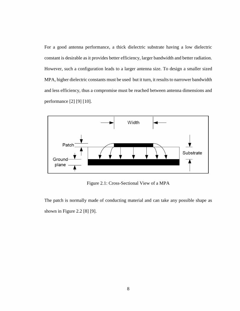
For a good antenna performance, a thick dielectric substrate having a low dielectric
constant is desirable as it provides better efficiency, larger bandwidth and better radiation.
However, such a configuration leads to a larger antenna size. To design a smaller sized
MPA, higher dielectric constants must be used but it turn, it results to narrower bandwidth
and less efficiency, thus a compromise must be reached between antenna dimensions and
performance [2] [9] [10].
Figure 2.1: Cross-Sectional View of a MPA
The patch is normally made of conducting material and can take any possible shape as
shown in Figure 2.2 [8] [9].

9
(a). Square (b). Rectangular (c). Circular(d). Elliptical
(e). Triangular (g). Disc Sector(f). Circular Ring (h) Ring Sector
Figure 2.2: Representative Shapes of MPAs
The rectangular shaped patch antenna is the most common type of MPAs because of its
ease in the analysis, fabrication, and its attractive radiation characteristics especially low
cross polarization radiation. The rectangular MPA is made of a rectangular patch with
dimensions width (W) and length (L) over a ground plane with a substrate thickness (h)
and dielectric constants ( r ) as shown in Figure 2.3 [7] [12].
Figure 2.3: Structure of a Rectangular MPA

10
2.1.3. Antenna Properties
2.1.3.1. Gain
This is the quantity which describes the capability of an antenna to concentrate power in
a given direction. In many instances, transmission is required between a transmitter and
only one receiving station. Power is thus radiated in one direction because it is useful only
in that direction. Transmitting and receiving antennas should have small power losses and
should be efficient as radiators and receptors. Gain is expressed in dB and is defined as
antenna directivity times a factor representing the radiation efficiency and its expression
is as follows;
G = η x D (2-1)
where, G – Gain, η – The efficiency of the antenna, and D – Directivity
2.1.3.2. Voltage Standing Wave Ratio (VSWR)
Voltage Standing Wave Ratio is a measure of impedance mismatch between the feeding
system and the antenna. Maximum power transfer can take place only when the input
impedance of the antenna is matched to that of the feeding source impedance [11]. The
higher the VSWR, the greater is the mismatch. The minimum possible value of VSWR is
unity and this corresponds to perfect match
1
1VSWR (2-2)

11
cL
cL
i
r
ZZ
ZZ
V
V
(2-3)
where, is the reflection coefficient, Vr is the amplitude of the reflected wave, Vi is the
amplitude of the incident wave, Zc is the characteristic impedance of the feeder cable, and
ZL is the load/antenna impedance.
2.1.3.3. Return Loss
Return loss (RL) is a ratio of power transferred to the load to power reflected back. To
obtain a perfect matching between the feeding system and the antenna; =0, and RL = -
infinity, thus no power is reflected back. RL is given as;
log20RL (dB) (2-4)
2.1.4. Microstrip Patch Antennas Polarization
The polarization of an antenna refers to the polarization of the electric field vector of the
radiated wave. It is the orientation of the electric fields as observed from the source versus
time. A transmit antenna needs a receiving antenna with the same polarization for
optimum operation [8]. Depending upon their geometry, MPAs can produce different
polarization. The common and typical types of polarization are the linear (horizontal or
vertical) and circular (right hand or the left hand) polarization [8] [13] [14].

12
2.1.4.1. Linear Polarization
Linearly polarized waves are defined with respect to a local ground plane as shown in
Figure 2.4. A horizontally polarized wave has an electric field vector that oscillates in a
direction parallel to the ground plane, while the electric field vector of a vertically
polarized wave has a component that is orthogonal to the ground plane. When the antenna
and wave polarizations are identical, the antenna extracts the maximum power from an
incident wave. On the other hand, no power can be received when the polarizations are
orthogonal to each other, as, for example, vertical and horizontal polarizations. Normally,
conventional rectangular MPAs are linearly polarized radiating structures [8] [13] [14].
Figure 2.4: Linearly Polarized Line-Fed MPA
2.1.4.2. Circular Polarization
Circular polarization (CP) is a result of orthogonally fed signal input. When two signals
of equal amplitude have 90° phases, the resulting wave is circularly polarized as show in

13
Figure 2.5. CP can result in left hand circularly polarized (LHCP) wave with
anticlockwise, or right hand circularly polarized (RHCP) wave with clockwise rotation.
The main advantage of CP is that regardless of receiver orientation, it will always be able
to receive a component of the signal. This reception is due to the resulting wave having
an angular variation [13] [14].
Figure 2.5: Circularly Polarized Line-Fed MPA
2.1.5. Advantages and Disadvantages of Microstrip Patch Antennas
In the recent past, the use of MPA in wireless communication has increased significantly.
This is mainly due to their low-profile structure amongst other merits. However, they do
possess a number of disadvantages as any other type of an antenna.

14
2.1.5.1. Advantages of Microstrip Patch Antennas
Some of the advantages of patch antennas as discussed in [7] [16] [14] [10] [15] are;
• Light weight and low volume.
• Low profile planar configuration easily made conformal to host surface.
• Low fabrication cost, hence mass production.
• Support of both linear and circular polarization.
• Capability of dual and triple frequency operations.
• Possibility of simultaneous fabrication of feed lines and matching network.
• Ease of integration with microwave integrated circuits (MICs).
2.1.5.2. Disadvantages of Microstrip Patch Antennas
Microstrip patch antennas suffer from a number of disadvantages as compared to
conventional antennas as discussed in [7] [16] [14] [10] [15], such as;
• Narrow bandwidth and low gain with low efficiency.
• Computational (numerical) intensive design with computer memory intensive
design softwares.
• Surface wave excitation and extraneous radiation from feeds and junctions
• Low power handling capacity.
• Complex feed structures requiring high performance arrays.

15
2.1.6. Microstrip Antennas Feed Techniques
MPAs can be fed by a variety of methods which are classified into two categories;
contacting and non-contacting. Contacting feed technique is where the power is fed
directly to the radiating patch through the connecting element such as microstrip line.
Non-contacting technique is where an electromagnetic magnetic coupling is done to
transfer the power between the microstrip line and the radiating patch. The most popular
contacting feed techniques used are the microstrip line feed and coaxial probe feed, while
the most popular non-contacting feed techniques are aperture coupling feed and proximity
coupling feed [12] [13].
2.1.6.1. Coaxial Probe Feed Technique
This is the most common feed technique used in the design of MPAs. As seen in Figure
2.6, the external or the outer conductor is connected to the ground plane and the inner
conductor of the coaxial connector extends through the dielectric and is soldered to that
of the radiating patch.
Figure 2.6: Coaxial Probe Feed Technique

16
Unlike the other feed techniques, coaxial probe feed has the flexibility of placing the feed
anywhere in the patch in order to match the input impedance. This gives an easy way for
the fabrication and it has low spurious radiation. The disadvantage of this type of feed is
the narrow bandwidth. Also with the extended or the increase probe length, the input
impedance becomes more inductive, which leads to the impedance matching challenges
[8] [12] [13].
2.1.6.2. Microstrip Line Feed Technique
This type of feed technique uses conducting strip that is directly connected to the edge of
the microstrip patch as shown in Figure 2.7. The conducting strip and the patch both can
be fabricated simultaneously on the same substrate to provide a planar structure. The
width of a conducting strip is smaller than that of the patch.
Figure 2.7: Microstrip Line Feed Technique

17
This method provides an easy and a simple way in the fabrication, modeling, and
especially in the impedance matching. However, the surface waves and the spurious feed
radiation increases as the thickness of the dielectric substrate increases which obviously
hampers the bandwidth of the antenna. Also, the serious drawbacks of this feed structure
are the strong parasitic radiation thus, it requires a transformer for impedance matching
which restricts the broadband capability of the antenna [8] [12] [13].
2.1.6.3. Aperture-Coupled Feed Technique
This type of method falls under the non-contacting feed techniques. In this type of feed
technique, the radiating patch and the microstrip feed line are divided by the ground plane
as shown in Figure 2.8.
Figure 2.8: Aperture-Coupled Feed Technique
On the bottom side of lower substrate, there is a microstrip feed line whose energy is
coupled to the patch through a slot on the ground plane separating two substrates. The

18
amount of coupling depends on the size, shape and also the location of the aperture.
Since the ground plane separates the patch and the feed line, spurious radiation is
minimized. Generally, a high dielectric material is used for the bottom substrate and a
thick, low dielectric constant material is used for the top substrate to optimize radiation
from the patch. The main outstanding feature in this particular feed technique is the
wider bandwidth. It has all of the advantages of the former two structures and it also
isolates the radiation from the feed network thereby leaving the main antenna radiation
uncontaminated. The major disadvantage of this feed technique is that it is difficult to
fabricate due to multiple layers, which also increases the antenna thickness [8] [13] [16].
2.1.6.4. Proximity-Coupled Feed Technique
This type of feed technique is also called the electromagnetic coupling scheme. As shown
in Figure 2.9, two dielectric substrates are used such that the feed line is in between the
two substrates and the radiating patch is on top of the upper substrate.
Figure 2.9: Proximity-Coupled Feed Technique

19
The main advantage of this feed technique is that it eliminates spurious feed radiation and
provides very high bandwidth (as high as 13%) [16]. This proximity-coupled feed
technique also provides choices between two different dielectric media; one for the patch
and one for the feed line to optimize the individual performances. Matching can be
achieved by controlling the length of the feed line and the width-to-line ratio of the patch.
The major disadvantage of this feed scheme is that it is difficult to fabricate because of
the two dielectric layers which need proper alignment. Also, there is an increase in the
overall thickness of the antenna [16] [12] [13].
Table 2.1 summarizes the characteristics of microstrip line feed, coaxial probe feed,
aperture-coupled feed, and proximity-coupled feed techniques [13] [16].
Table 2.1: Comparison of Different Feed Techniques
Characteristics Coaxial
Probe Feed
Microstrip
Line Feed
Aperture-
Coupled Feed
Proximity-
Coupled Feed
Configuration Non Planar Coplanar Planar Planar
Ease of
Fabrication
Soldering and
drilling
needed
Easy Alignment
required
Alignment
required
Spurious Feed
Radiation
More More Less Minimum
Reliability Poor due to
soldering
Better Good Good
Impedance
Matching
Easy Easy Easy Easy
Polarization
Purity
Poor Poor Excellent Poor
Bandwidth 2-5% 2-5% About 15% About 13%

20
2.1.7. Application of Microstrip Patch Antennas
The usage of the MPAs is spreading widely in both commercial and non-commercial
aspects due to the low cost of the substrate material and ease of fabrication, with the most
applications being on mobile communication systems. MPAs are mostly applicable where
small, lightweight, low profile, and low‐cost conformal structures are required. As
discussed in [8] [10] [13] [16], some of the applications include;
2.1.7.1. Mobile and Satellite Communication Application
MPAs are widely used in mobile communication systems. An example is shown in the
Figure 2.10. In the case of satellite communication, circularly polarized radiation patterns
are usually used and can be realized using either square or circular patch with one or two
feed points.
Figure 2.10: MPA in a Cellular Phone
Other applications of MPAs include the following among others;

21
2.1.7.2. Global Positioning System Application
MPAs are used for global positioning system due to its ease in integration of a low noise
amplifier on the substrate used for the feeding circuitry. These antennas are usually
circularly polarized. Most of the GPS receivers are used by the general population for land
vehicles, aircraft, and maritime vessels.
2.1.7.3. Radio Frequency Identification (RFID)
RFID systems consist of a tag or transponder and a transceiver or reader RFID and are
used in different areas like mobile communication, logistics, manufacturing,
transportation, and health care. They generally use frequencies between 30 Hz and 5.8
GHz depending on its applications.
2.1.7.4. Worldwide Interoperability for Microwave Access
(WiMAX)
Microstrip patch antennas are used for WiMAX as they meet the IEEE 802.16 standard
[14].
2.1.7.5. Radar Application
Radar can be used for detecting moving targets such as people and vehicles. It demands a
low profile light weight antenna subsystem making MPAs the most ideal choice.

22
2.1.7.6. Telemedicine Application
In telemedicine application, the antennas mostly used operate at 2.45 GHz. A semi
directional radiation pattern is preferred over the omni-directional pattern to overcome
unnecessary radiation to the user's body, thus MPAs are suitable for telemedicine
applications. Also, it has been proved that in the treatment of malignant tumors,
microwave energy is the most effective way of inducing hyperthermia [16]. The design
of the particular radiator which is to be used for this purpose should posses light weight,
easy in handling, and to be rugged and therefore, the patch radiator fulfils these
requirements.

23
2.2. Artificial Intelligence Techniques
Artificial intelligence (AI) is the ability of a computer or any other machine to perform
those activities that are normally thought to require intelligence by evaluating information
and making decisions according to pre-established criteria. AI borrows its meaning from
the word intelligence which is defined as the ability to apply past and present experience
to satisfactorily solve present and future problems. In AI, the basic paradigm of intelligent
action is that of searching through a space of partial solutions (called the problem space)
for a goal situation. Fuzzy logic, artificial neural networks, genetic algorithms, and
particle swarm optimization, among others are examples of AI techniques that are
applicable in every day’s life [17] [22]. Artificial intelligence techniques have gained
popularity in engineering design in recent years due to their efficiency and effectiveness
[22]. Various papers have been published in the recent past on the design of antennas
using AI techniques as seen in [2] [15] [26] [33] [36].
2.2.1. Fuzzy Logic
Fuzzy logic is a form of multi-valued logic derived from fuzzy set theory to deal with
reasoning that is approximate rather than precise. It is a problem-solving control system
methodology that deals with the use of logical rules to solve nonlinear and complex
problems by employing the use of linguistic terms that deal with the causal relationship
between the input and output variables, thus treating the variables as continuous rather
than discrete [22]. This system is implemented in MATLAB® Fuzzy Toolbox. Various

24
researches have shown that human thinking does not always follow crisp “yes”/“no” logic,
but rather it is often vague, qualitative, uncertain, imprecise, or fuzzy in nature. Therefore,
fuzzy system provides parameters of the fuzzy control paradigm which is a collection of
rules and fuzzy set membership functions [18] [19]. Among the reasons for using fuzzy
logic technique is that it;
Is conceptually easy to understand.
Is flexible.
Is tolerant of imprecise data.
Can be blended with conventional control techniques.
Is based on natural language.
2.2.1.1. Fuzzy sets
Fuzzy set is classification of a set without crisp or clearly defined boundary. Fuzzy set
can contain elements with only a partial degree of membership. Unlike classical set based
on Boolean logic, a particular object has a degree of membership in a given set that may
be anywhere in the range of 0 (completely not in the set) to 1 (completely in the set), thus,
it is often defined as multi-valued logic (or 0-1) [18].

25
2.2.1.2. Membership Functions
A membership function (MF) is a curve that defines how each point in the input space is
mapped to a membership value (or degree of membership) between 0 and 1. A fuzzy set
can be defined by enumerating membership values of the elements in the set if it is discrete
or by defining the membership function mathematically if it is continuous. Although there
exist numerous types of membership functions, the most commonly used in practice are
triangles, trapezoids, Gaussian, and bell curves [19] [20].
2.2.1.3. Fuzzy If-Then Rules
Fuzzy if-then rules are a knowledge representation scheme for capturing knowledge
(typically human knowledge) that is imprecise and inexact by nature. Generally, this is
achieved by using linguistic variables to describe elastic conditions (that is, conditions
that can be satisfied to a degree) in the “if” part of fuzzy rules and to perform inference
under partial matching. A fuzzy if-then rule takes the form:
IF x is Ak THEN y is Bk (x) (2-5)
where, Ak and Bk are linguistic values defined by fuzzy sets on universes x and y
respectively. Often, the “if” part is called antecedent or premise, while the “then” part is
called consequence or conclusion. The fuzzy sets in a rule’s antecedent define a fuzzy
region of the input space covered by the rule (that is, the input situations that fit the rule’s

26
condition completely or partially), whereas the fuzzy sets in a rule’s consequent describe
the vagueness of the rule’s conclusion [18] [20].
2.2.1.4. Fuzzy Inference Systems (FIS)
Fuzzy inference is the actual process of mapping from a given input to an output using
fuzzy logic. A typical FIS consists of membership functions, a rule base and an inference
procedure. The basic structure of a FIS consists of three conceptual components:
i. A rule base, which contains a selection of fuzzy rules;
ii. A database, which defines the membership functions used in the fuzzy rules;
iii. A reasoning mechanism, which performs the inference procedure upon the
rules and given facts to derive a reasonable output or conclusion.
The inputs of fuzzy inference system can either be fuzzy sets or crisp values (which are
viewed as fuzzy singletons). If the system produces fuzzy sets as output while a crisp
output is needed, then a method of defuzzification is required to extract a crisp value that
best represents the fuzzy set [18] [20].
Depending on the types of fuzzy reasoning and fuzzy if-then rules employed, most fuzzy
inference systems can be classified into two types namely Mamdani and Sugeno fuzzy
models.

27
2.2.1.4.1. Mamdani Fuzzy Model
Mamdani fuzzy model was proposed Mamdani (1975) [19] as an attempt to control a
steam engine and boiler combination by a set of linguistic control rules. A Mamdani fuzzy
system uses fuzzy sets as rule consequent. The fuzzy rule in this model is in the form of:
IF x1 is Ai1…and/or xn is Ain THEN y is Ci (2-6)
where, xj (j=1, 2… n) are the input variables, y is the output variable, and Aij and Ci are
fuzzy sets for xj and y respectively [19] [20].
2.2.1.4.2. Sugeno Fuzzy Model
Sugeno fuzzy model was proposed by Takagi, Sugeno, and Kang [19] in an effort to
develop a systematic approach of generating fuzzy rules from a given input-output data
set. A typical two-input fuzzy rule in this model is in the form of:
IF x1 is A and x2 is B THEN y = f(x1, x2). (2-7)
where, A and B are fuzzy sets in the antecedent and y = f(x1, x2) is a crisp function in the
consequent. Usually, f(x1, x2) is a polynomial function of the input variables x1 and x2,
but it can be any function as long as it can appropriately describe the output of the model
within the fuzzy region specified by the antecedent of the rule. When f(x1, x2) is a first-
order polynomial function, the resulting fuzzy inference system is called a first-order
Sugeno fuzzy model. When f(x1, x2) is a constant, the system is referred as a zero-order
Sugeno fuzzy model [19] [20]. Because it is a more compact and computationally efficient

28
representation than a Mamdani system, the Sugeno system lends itself to the use of
adaptive techniques for constructing fuzzy models. These adaptive techniques can be used
to customize the membership functions so that the fuzzy system best models the data.
2.2.2. Artificial Neural Networks
Artificial Neural Network (ANN) is information processing technique with the capability
of performing computations similar to human brain or biological neural network. ANN is
a technique that seeks to build an intelligent program to implement intelligence similar to
that of a human brain processing. ANN uses models that simulate the inter-connection of
neurons, such that neuron outputs are connected (through weights), to all other neurons
including themselves. Just like the way human brain remembers and learns, an ANN
system works in a similar manner. With the set of input data patterns, the network can be
trained (not programmed) to give corresponding desired patterns at the output [21] [22].
Some of the reasons why this AI technique has gained popularity are;
Their ability to derive meaning from complicated or imprecise data
Adaptive learning: An ability to learn how to do tasks based on the data given for
training or initial experience.
Self-Organization: An ANN can create its own organization or representation of
the information it receives during learning time.
Real Time Operation: ANN computations may be carried out in parallel with
simulations.

29
Parallel Computation: ANN is a fast and massive parallel input parallel output
multidimensional computing system.
Learning methods used for ANN can be classified into two major categories namely
supervised and unsupervised learning.
2.2.2.1. Supervised Learning
The goal of supervised learning is to shape the input-output mappings of the network
based on a given training data set. As the term suggests, first, the desired input-output data
sets must be known; then the resulting networks need to have adjustable parameters that
are updated by a supervised learning rule. The adjustable parameters are often referred to
as weights. In supervised training, both the inputs and the outputs are provided. The
network then processes the inputs and compares its resulting outputs against the desired
outputs. Errors are then propagated back through the system, causing the system to adjust
the weights which control the network. This process occurs over and over as the weights
are continually tweaked [22]. The set of data which enables the training is called the
‘training set’. During the training of a network, the same set of data is processed many
times as the connection weights are ever refined. An important issue concerning
supervised learning is the problem of error convergence, that is, the minimization of error
between the desired and computed unit values. The aim is to determine a set of weights
which minimizes the error [23].

30
Back-propagation (BP), also known as back error propagation or the generalized delta
rule is an example of supervised learning method. The training process involves two steps;
a forward propagating step and a backward propagating step. In the forward pass, the
training input data is presented to the input layer. The data propagates on through the
hidden layers, until it reaches the output layer, where it is displayed as the output pattern.
In the backward pass, the error term is calculated and propagated back to change the
assigned weights of the inputs. The magnitude of the error value indicates how large an
adjustment needs to be made and the sign of the error value gives the direction of the
change [24].
2.2.2.2. Unsupervised Learning
In unsupervised training, the network is provided with inputs but not with desired outputs.
The system itself must then decide what features it will use to group the input data. This
is often referred to as self-organization or adaption. Unsupervised learning is learning with
no information available regarding the desired outputs; the network updates weights only
on the basis of the input patterns. Self-organizing implies the ability to acquire knowledge
through a trial and error learning process involving organizing and reorganizing in
response to external stimuli [22] [24]. Kohonen self-organizing maps also known as
Kohonen self-organizing feature maps, are one of the common unsupervised learning
paradigms [24].

31
2.2.3. Neuro-Fuzzy Systems
Neural networks and fuzzy logic are two complementary technologies as discussed earlier.
This is because neural networks have the learning ability which can learn knowledge using
training examples, while fuzzy inference systems can deduce knowledge from the given
fuzzy rules. Therefore, the combination of these two outperforms either neural network
or fuzzy logic method used exclusively [25]. Fast and accurate learning, excellent
explanation facilities in the form of semantically meaningful fuzzy rules, the ability to
accommodate both data and existing expert knowledge about the problem, and good
generalization capability features have made neuro-fuzzy systems popular in the recent
past [23] [24].
2.2.3.1. Adaptive Neuro-Fuzzy Inference System (ANFIS)
Fundamentally, ANFIS is about taking a FIS and tuning it with an ANN algorithm based
on some collection of input-output data. Using a given input/output data set, the toolbox
function ANFIS constructs a FIS whose membership function parameters are tuned
(adjusted) using either a back-propagation algorithm alone or in combination with a least
squares type of method. This adjustment allows the fuzzy systems to learn from the data
they are modeling [24] [28]. The parameters associated with the membership functions
changes through the learning process. The computation of these parameters (or their
adjustment) is facilitated by a gradient vector. This gradient vector provides a measure of
how well the fuzzy inference system is modeling the input/output data for a given set of

32
parameters. When the gradient vector is obtained, any of several optimization routines can
be applied in order to adjust the parameters and to reduce some error measure. This error
measure is usually defined by the sum of the squared difference between actual and
desired outputs [25] [29]. This process is referred as supervised learning in neural network
literature. By combining the advantages of imprecise data sampling of fuzzy logic and the
intelligence of ANN, the neuro-fuzzy outsmarts the two AI and therefore, this AI method
was chosen for this work so as to show that it can be used to design MPAs with the results
that are in agreement with the conventional design results.
2.2.3.2. Architecture of Adaptive Neuro-Fuzzy Inference System
ANFIS network is organized into two parts like fuzzy systems. The first part is the
antecedent and the second part is the conclusion, and the two are connected to each other
by rules to form a network. A step in the learning process has two passes: In the first pass,
training data is brought to the inputs while the premise parameters are assumed to be fixed
and the optimal consequent parameters are estimated by an iterative least mean square
procedure. In the second pass, the patterns are propagated again but this time the
consequent parameters are assumed to be fixed and back-propagation is used to modify
the premise parameters [28] [25]. The process will repeat itself depending on the number
of epochs (iterations) specified.

33
The ANFIS architecture consists of five layers namely; fuzzy layer, product layer,
normalized layer, de-fuzzy layer, and summation (total output) layer as shown in Figure
2.11. In the figure, a circle indicates a fixed node, whereas a square indicates an adaptive
node [8].
A1
B2
B1
A2
Prod
Sum
Norm
Norm
Prod
x
y
Layer
1
Layer
2
Layer
3
Layer
4Layer
5
f
x
x
y
y
O1,i
O2,i O3,i
O4,i
Figure 2.111: Architecture of an ANFIS
Assume that the fuzzy inference system under consideration has two inputs x and y and
one output f. Based on a first-order Sugeno model, a typical rule set with two fuzzy if-
then rules can be expressed as;
Rule1: If x is A1 and y is B1, then f1 = p1x + q1y + r1 (2-8)
Rule2: If x is A2 and y is B2, then f2 = p2x + q2y + r2 (2-9)
where, A1, B1, A2, B2 are fuzzy sets, pi, qi and ri (i = 1, 2) are the coefficients of the first-
order polynomial linear functions.

34
The following section discusses in depth the relationship between the input and output of
the five layers in ANFIS architecture as outlined in [20] [26] [27] [28].
Layer 1 is the Fuzzy Layer, in which x and y are the input of nodes A1, B1, and A2, B2
respectively. A1, B1, A2, and B2 are the linguistic labels used in the fuzzy theory for
dividing the membership functions. The membership relationship between the output and
input functions of this layer can be expressed as;
),(,1 xOiAi i = 1, 2 (2-10)
),(,1 yOjBi
j = 1, 2 (2-11)
where O1,i and O1,j denote the output functions, whereas μAi and μBj denote the
membership functions respectively.
Layer 2 is the Product Layer that consists of two nodes labeled Prod. The output w1 and
w2 are the weight functions of the next layer. Each node calculates the firing strength of a
rule via multiplication. The output of this layer (O2,i) is the product of the input signal,
and is defined as;
),()(,2 yxwOji BAii
i, j = 1, 2 (2-12)
Layer 3 is the Normalized Layer whose nodes are labeled Norm. Its function is to
normalize the weight function, that is, the firing strength from previous layer. It calculates
the ratio of the ith rule’s firing strength to the sum of the entire rule’s firing strengths. The
output is denoted as O3,i and is defined in Eq. 2-13.

35
2,1,,21
3
iww
wwO i
ii (2-13)
Layer 4 is the De-fuzzy Layer whose nodes are adaptive. pi, qi and ri denote the linear
parameters which are also called consequent parameters of the node. The de-fuzzy
relationship between the input and output of this layer can be defined as Eq. 2-14, where
O4,i denotes the Layer 4 output. The output of each node is simply the product of the
normalized firing strength and a first order polynomial.
)(,4 iiiiiii ryqxpwfwO (2-14)
Layer 5 is the Total Output Layer whose single node is labeled as Sum. The output of
this layer denoted as O5,I, is the total of input signals. The results can be expressed as;
i
i
i
ii
i
ii
w
fw
fwO 15 , (2-15)
The output of ANFIS can be therefore, be written as;
2
21
21
21
1 fww
wf
ww
wf
(2-16)
Substituting Eq. 2-13 into Eq. 2-16 yields
2211 fwfwf (2-17)
Substituting the fuzzy if-then rules in Eq. 2-8 and 2-9 into Eq. 2-17, then yields
)()( 22221111 ryqxpwryqxpwf (2-18)

36
The output can therefore, be expressed as a linear combination of the consequent
parameters:
))()()()( 222222111111 rwqywpxwrwqywpxwf
(2-19)
In this ANFIS architecture, there are two adaptive layers (layer 1 and 4). Layer 1 has
modifiable parameters pertaining to the input MFs. These parameters are called premise
parameters. Layer 4 has three modifiable parameters (pi, qi and ri) pertaining to the first
order polynomial. These parameters are called consequent parameters [28].
2.2.3.3. ANFIS Learning Technique
To identify the parameters in the nonlinear neuro-fuzzy model, the gradient descent
method [25] in conjunction with error BP process [25] [26] could be used for neural
network learning. However, this optimization method usually takes a long time to
converge. An alternative is the Least-Squares Method (LSM) which is a powerful and
well developed tool that is widely employed in areas such as adaptive control, signal
processing and statistics. The hybrid learning algorithm combining the LSM and the BP
algorithm can be used to solve the problem of convergence. This algorithm converges
much faster, since it reduces the dimension of the search space of the BP algorithm [25]
[18]. During the learning process, the premise parameters in the layer 1 and the consequent
parameters in the layer 4 are tuned until the desired response of the FIS is achieved. The

37
hybrid learning algorithm is a two-step process. First, while holding the premise
parameters fixed, the functional signals are propagated forward to layer 4, where the
consequent parameters are identified by the LSM. Then, the consequent parameters are
held fixed while the error signals, the derivative of the error measure with respect to each
node output, are propagated from the output end to the input end, and the premise
parameters are updated by the standard BP algorithm. This process is repeated until the
results are deemed satisfactory (when the error becomes zero) or once the process reaches
a specified epoch number [10] [26].

38
CHAPTER THREE
3.0. DESIGN METHODOLOGY
3.1. Rectangular Microstrip Antenna Design
The rectangular MPA is made of a rectangular patch with dimensions width (W) and
length (L) over a ground plane with a substrate thickness (h) and dielectric constant ( r ).
This work concentrates only on the basic geometry of the MPAs ignoring the various
complex structures adopted for the enhancement of bandwidth, directivity, and gain.
3.2. Design Specifications
There are various methods of analysis for MPAs namely; transmission-line, cavity, and
full-wave (methods of moments). In this thesis, the transmission-line method is used as it
gives good physical insight and is easy to model. Figure 3.1 shows the electric fields of a
basic rectangular MPA.
Radiating
Patch
Dielectric
Substrate
Ground
Plane
Electric
Fields
Figure 3.1: MPA Electric Field Lines

39
The transmission-line method is the most commonly used method in the design of
rectangular MPAs. The steps followed in the design of rectangular MPAs as discussed in
[7] [8] [12] [35] are as follows;
Step 1: Calculating the Patch Width (W) – For efficient radiation, the patch width W is
given as;
1
2
2
rrf
cW
(3-1)
where, W is the Patch width, c is the speed of light, fr is the resonant frequency, and r is
the dielectric constant of the substrate.
Step 2: Calculating the Effective Dielectric Constant ( reff ) – As seen in Figure 3.1, most
of the electric field lines reside in the substrate and parts of some lines in air. An effective
dielectric constant (εreff) must be obtained in order to account for the fringing effect and
the wave propagation in the line.
2
1
1212
1
2
1
W
hrrreff
(3-2)
where, εreff is the effective dielectric constant and h is the height of the dielectric substrate.
Step 3: Calculating the Effective Length ( effL ) – For a given resonance frequency fr, the
effective patch length is given as;

40
reffr
efff
cL
2 (3-3)
where, effL is the effective length.
Step 4: Determining the Length Extension ( L ) – The fringing fields along the width
can be modeled as radiating slots and electrically, the patch of the MPA looks greater than
its physical dimensions. The dimensions of the patch along its length have now been
extended on each end by a distance ΔL, which is given as;
8.0258.0
264.03.0
412.0
h
W
h
W
hL
reff
reff
(3-4)
where, ΔL is the patch length extension.
Step 5: Determining the Patch Length (L) – The actual patch length now becomes;
L Leff - 2 L (3-5)
where, L is the actual patch length.
Step 6: Calculating the Bandwidth (BW)
%100*
177.3%
2
or
r h
L
WBW
(3-6)
where, o is the wavelength in free space.

41
Step 7: Determining the Feed Co-ordinates – Using coaxial probe-fed technique, the feed
points are calculated as;
Yf = W/2 (3-7)
reff
f
Lx
2 (3-8)
where, Yf and Xf are the feed co-ordinates along the patch width and length respectively
Step 8: Determining the Plane Ground Dimensions – It has been shown that MPAs
produces good results if the size of the ground plane is greater than the patch dimensions
by approximately six times the substrate thickness all around the periphery [35] [37].
Lg = 6h + L (3-9)
Wg = 6h + W (3-10)
where, Lg and Wg are the plane ground dimensions along the patch length and width
respectively
3.3. Application of ANFIS in the design of a Rectangular Microstrip
Patch Antenna
As discussed in Chapter 2, ANFIS uses a set of data for training of its network. There are
two types of data generators (measurements and simulations) for antenna applications.
The selection of a data generator depends on the application and the availability of the
data generator. In this work, the ANFIS model shown in Figure 3.2 with the inputs
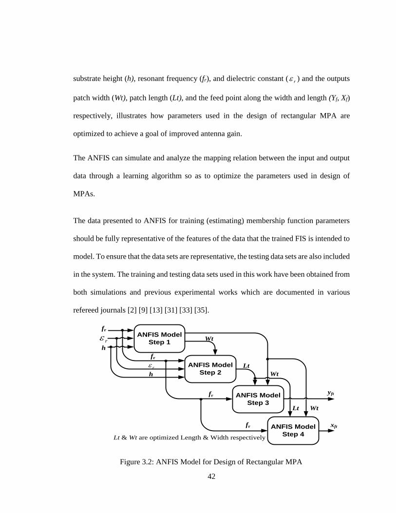
42
substrate height (h), resonant frequency (fr), and dielectric constant ( r ) and the outputs
patch width (Wt), patch length (Lt), and the feed point along the width and length (Yf, Xf)
respectively, illustrates how parameters used in the design of rectangular MPA are
optimized to achieve a goal of improved antenna gain.
The ANFIS can simulate and analyze the mapping relation between the input and output
data through a learning algorithm so as to optimize the parameters used in design of
MPAs.
The data presented to ANFIS for training (estimating) membership function parameters
should be fully representative of the features of the data that the trained FIS is intended to
model. To ensure that the data sets are representative, the testing data sets are also included
in the system. The training and testing data sets used in this work have been obtained from
both simulations and previous experimental works which are documented in various
refereed journals [2] [9] [13] [31] [33] [35].
ANFIS Model
Step 1
ANFIS Model
Step 3
ANFIS Model
Step 2
r
r
fr
fr
fr
h
h
yft
Wt
Wt
Lt
Lt & Wt are optimized Length & Width respectively
ANFIS Model
Step 4
WtLt
xft fr
Figure 3.2: ANFIS Model for Design of Rectangular MPA

43
3.4. ANFIS Design Procedure
Figure 3.3 is an optimization design procedure followed in this work. Using MATLAB®,
a program was developed comprising of the design formulas illustrated in Eq. 3-1 to Eq.
3-10. This program (Appendix A-1) was then used to generate the data sets for training of
ANFIS. Here, all the formulas used in designing of basic rectangular MPA were put into
consideration. The program allows for computer human interaction as it allows the user
to input specific resonant frequency, substrate height, and dielectric constant of a specific
material under consideration. The generated data comprising of design parameters were
saved to be used in optimizing the patch dimensions data at a later stage. In the second
step, a program containing test data sets available in literature from the previous
experimental works published in several sources ([2] [9] [10] [13] [26] [31] [33] [35] [36])
was developed as shown in Appendix A-2. These test data sets are arranged in a matrix
format depending on the number of parameters to be used in the optimization procedure.
Another MATLAB® program with the ANFIS model for optimizing parameters was
developed as shown in Appendix A-3. In this program, the membership function type and
number is specified beforehand together with the number of epochs for training. The
optimization using ANFIS can be illustrated in a flowchart in Figure 3.3 where the output
can be achieved once the specified number of epochs is achieved or the error becomes
zero.

44
Program 1 – For
Generating MPA
Dimensions
User Input (Interface)
Initialize with
Random Weights
Training
Data Sets
Testing
Data Sets
Training
Network
Testing
Network
Error Acceptable/
Epoch Reached
Output – Optimized
Patch Dimensions
Program for Generating Training Data Sets
AN
FIS
Op
tim
izat
ion
Pro
gra
m
Y
NY and N means yes
and no respectively
Figure 3.3: Flowchart for Optimization of Rectangular MPA
As illustrated in Figure 3.2, the ANFIS model contains four stages. In the first stage,
resonant frequency, dielectric constant, and substrate height are used in optimizing the
patch width (W) of the antenna. 90 data sets were used for training while 18 data sets were
used as test data sets as shown in Appendix B-1. The MFs for the input variables fr, r ,
and h, are 4, 3, and 3 respectively. The number of rules is then 36 (4x3x3) and the number

45
of epochs specified as 700. In the second stage, the antenna patch length (L) is optimized.
The three input variables used in first stage are maintained with the addition of the
optimized patch width (Wt) as an input variable, therefore, variables fr, r , h, and Wt are
used as inputs with L as the output variable to be optimized. 90 training and 16 testing
data sets shown in Appendix B-2 were used in this stage. The MFs for the input variables
fr, r , h, and Wt are 4, 2, 2, and 4 respectively thus, the number of rules is 64 (4x2x2x4)
with the number of epochs specified as 700. The third stage in the ANFIS model is used
for optimizing the feed point (Yf) along the patch width. In this stage, the number of epochs
is specified as 600 with 90 testing data sets and 15 testing data sets (Appendix B-3) used.
The variables fr, Wt, and Lt are used as inputs with the MFs as 3, 4, and 4 respectively.
This gives the number of rules as 48 (3x4x4). Finally, the input variables fr, Wt, and Lt are
used in optimizing the feed point Xf along the path length of the antenna. With 90 testing
data sets and 15 testing data (Appendix B-3) used, the number of iterations was specified
as 600. The input variables fr, Wt, and Lt were each allocate the MFs values as 3, 4, and 4
respectively, making the number of rules as 48 (3x4x4).
Figure 3.3 shows the procedure of generating the optimized parametric data. These data
are based on optimizing the antenna gain which is explained in the next chapter.
After running the above mentioned MATLAB® program and the optimized parameter
values noted down (see Appendix C), commercial antenna design software was then used
to design an antenna and the parameter values noted down. Finally, the two pairs of
rectangular microstrip patch antennas were fabricated based on the results.

46
CHAPTER FOUR
4.0. RESULTS AND DISCUSSIONS
The simulation results that were obtained by using Antenna Magus software (a product
of Magus (Pty) Ltd) to validate the performance of the proposed ANFIS model for
design of rectangular microstrip patch antennas is presented. Two sets of antennas (one
set based on ANFIS model and the other Antenna Magus software results respectively)
were fabricated in the lab and their performance characteristics experimentally measured
and analyzed. Two sets of rectangular MPAs were fabricate so as to compare the results
based on the design method (ANFIS and Antenna Magus Simulations).
4.1. ANFIS Simulation Results
As illustrated in Figure 3.2, ANFIS model used in this work has four stages. In each stage,
optimization is carried out as per the specified number of epochs. Using the Eq. 3-1 to 3-
10, training data sets were generated. Testing data sets were also collected (from refereed
journals and simulations as indicated in Chapter 3) and the overall ANFIS design model
formulated. Since ANFIS model is singleton (has one output), four similar design stages
were formulated. Finally, in order to view the rectangular MPA characteristic based on
the optimized parameters, Ansoft HFSS (High Frequency Structure Simulator) software
was fed with the optimized results.

47
In every microstrip patch antenna design, the resonant frequency and substrate material
type used are crucial in determining other physical parameters. Figure 4.1 illustrates the
first stage indicating the number of variables used.
Figure 4.1: First Stage of ANFIS Model
As illustrated earlier, the membership values were specified such that the total number of
rules was 36. At the end of the training, the root mean square error (RMSE) was 0.5180
at epoch number 700. The optimized patch width was then used in optimization in the next
stage.

48
Figure 4.2: Second Stage of ANFIS Model
The second stage of ANFIS model produced an optimized patch length. With four variable
(shown in Figure 4.2) specified as inputs, optimization was carried out resulting in an
RMSE error of 0.0052. Figure 4.3 shows how the input and output variables were arranged
in the third stage.

49
Figure 4.3: Third Stage of ANFIS Model
Figure 4.4: Fourth Stage of ANFIS Model

50
Figure 4.3 and Figure 4.4 shows how the variables used in optimization of feed point along
the patch width and length were carried out respectively.
With the emphasis on FR4 Glass-Epoxy substrate (with dielectric constant of 4.35 and
substrate height of 1.6mm) operating at 2GHz, various substrates (FR4 Glass-Epoxy,
Duroid 5880, DiClad880, Silicon, and Alumina substrates) were used in determining the
best possible parametric values for rectangular microstrip patch antenna. Figure 4.5 to 4.8
plots various optimized parameters with relation to resonant frequency. As mentioned
earlier, the program allows for human interaction therefore, in this work, quartz substrate
material with dielectric constant of 3.8 and substrate thickness of 1.5mm was used for
testing purposes and labeled as input in subsequent figures. Quartz substrate was chosen
as its dielectric constant value falls on the lower side of the dielectric constant value range
of 2.2 to 12, and also the lower the dielectric constant the higher the antenna gain and
bandwidth. [37].

51
Figure 4.5: ANFIS Optimized Patch Width vs Resonant Frequency
Figure 4.6: ANFIS Optimized Patch Length vs Resonant Frequency

52
Figure 4.7: ANFIS Optimized Feed Point along Patch Width vs Resonant Frequency
Figure 4.8: ANFIS Optimized Feed Point along Patch Length vs Resonant Frequency

53
As depicted in Figure 4.5 to Figure 4.8, the patch dimensions vary as per the type of
substrate material used in relation to resonant frequency. To plot the above rectangular
MPA optimized parameters, the substrates Duroid 5880 with dielectric constant of 2.2 and
substrate thickness of 1.57mm, FR4 Glass-Epoxy with substrate thickness of 1.6mm and
dielectric constant of 4.35, aluminum with dielectric constant of 9.8 and substrate
thickness of 1.5mm, and quartz with dielectric constant of 3.8 and substrate thickness of
1.5mm were used. Also, it can be seen that the higher the resonant frequency the smaller
the patch antenna therefore, it is not practical to use this type of an antenna for operational
frequencies above 6GHz because the fabrication process for relatively small sized
antennas is quite difficult and its power handling capability is greatly reduced.
Table 4.1: Summary of ANFIS Model Variables
ANFIS
Stage
Output
Variable
Input
Variables
RMSE
Prediction
1 Wt fr, r , h 0.5180
2 Lt fr, r , h, Wt 0.0052
3 Yft fr, Wt, Lt 0.0194
4 Xft fr, Wt, Lt 0.1770
Table 4.1 shows a summary of some of the specified design parameters and the output
RMSE. The error goal was set at default 0 with the initial step size set at 0.04 and the
decrease and increase step size learning rate set at 0.9 and 1.1 respectively. Due to the
specification of the Antenna Trainer Kit used for testing the MPA, the rectangular MPA
was designed with the operating frequency of 2GHz. Table 4.2 shows the ANFIS

54
optimized MPA design parameters which were used in fabricating the antenna. This data
is extracted from the results table on Appendix C, row 18. As indicated earlier, FR4 Glass-
Epoxy substrate material was used due to its availability.
Table 4.2: ANFIS Optimized Patch Antenna Design Parameters
fr 2 GHz Wt 46.818mm Xft 8.819mm
r 4.35 Lt 35.631mm Wg 55.456mm
h 1.6mm Yft 22.927mm Lg 45.241mm
To check the ANFIS designed patch antenna characteristics, the optimized parameters
namely; patch width, patch length, and feed point were fed onto HFSS simulation tool.
The resonant frequency was specified as 2GHz.
Figure 4.9: Return Loss of Rectangular MPA
1.00 1.25 1.50 1.75 2.00 2.25 2.50 2.75 3.00Freq [GHz]
-20.00
-17.50
-15.00
-12.50
-10.00
-7.50
-5.00
-2.50
0.00
dB
(St(
1,1
))
Patch_Antenna_ADKv1Return Loss ANSOFT
Curve Info
dB(St(1,1))Setup1 : Sw eep1
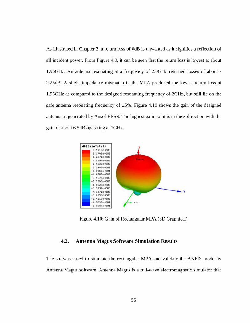
55
As illustrated in Chapter 2, a return loss of 0dB is unwanted as it signifies a reflection of
all incident power. From Figure 4.9, it can be seen that the return loss is lowest at about
1.96GHz. An antenna resonating at a frequency of 2.0GHz returned losses of about -
2.25dB. A slight impedance mismatch in the MPA produced the lowest return loss at
1.96GHz as compared to the designed resonating frequency of 2GHz, but still lie on the
safe antenna resonating frequency of ±5%. Figure 4.10 shows the gain of the designed
antenna as generated by Ansof HFSS. The highest gain point is in the z-direction with the
gain of about 6.5dB operating at 2GHz.
Figure 4.10: Gain of Rectangular MPA (3D Graphical)
4.2. Antenna Magus Software Simulation Results
The software used to simulate the rectangular MPA and validate the ANFIS model is
Antenna Magus software. Antenna Magus is a full-wave electromagnetic simulator that

56
is widely used in conjunction with FEKO software and used in the design of patch
antennas, wire antennas, and other RF/wireless antennas.
On specifying the frequency of 2GHz, substrate height of 1.6mm, and dielectric constant
of 4.35, simulation was carried out to establish the antenna parameters and characteristics
for a FR4 substrate. Table 4.3 shows the antenna parameters values as simulated on
Antenna Magus.
Table 4.3: Simulated Patch Antenna Design Parameters
fr 2 GHz W 45.825mm Xf 12.749mm
r 4.35 L 35.243mm Wg 91.649mm
h 1.6mm Yf 22.913mm Lg 70.486mm
On comparison between Table 4.2 and 4.3, a significant difference was noted on the
values of Xf, Wg, and Lg. This can be attributed to the type of formulas Antenna Magus
software is based on and the ANFIS model design procedure followed. A significant
difference in patch width, length, and feed point will affect the antenna performance, but
a variation in ground plane (Wg and Lg) should not affect the antenna performance so long
as the minimum ground plane is larger than six times the substrate height plus the
corresponding patch dimension as shown in Eq. 3-9 and 3-10. In Table 4.2, the
transmission-line method was used in the design procedure, while a full-wave
electromagnetic simulator Antenna Magus software was used to simulate the results in
Table 4.3.

57
Figure 4.11: VSWR of Rectangular Microstrip Patch Antenna at 2GHz
As discussed in the literature review, the value of VSWR should always be less than 2 for
proper operation of MPA. As shown in Figure 4.11 from Antenna Magus software
simulation, this MPA functions well within the frequency range of approximately
1.971GHz and 1.989GHz where the VSWR is less than 2. VSWR is minimum (1.107) at
a frequency of 1.98GHz. From Figure 4.11, VSWR at exactly 2GHz is about 4, and
therefore, a significant transmitted power loss. This loss can be greatly attributed to the
impedance mismatch. Applying Eq. 2.2 and a VSWR of 4, yields a return loss of 4.44dB.
On comparison between -2.5dB return loss from Figure 4.9 and 4.44dB from Figure 4.11,
it can be seen that the later has higher return losses that the former.

58
Figure 4.12: Gain of Rectangular MPA at 2GHz (3D Graphical Plot)
Figure 4.12 show the gain of a rectangular MPA as simulate on Antenna Magus software.
The gain is maximum (about 6dB) at a frequency of about 2.04GHz. From Figure 4.10,
the gain was found to be around 6.5dB on simulating the ANFIS parametric values on
Ansoft HFSS software. Similarly, Antenna Magus simulated software was used to
validate the ANFIS results and the results (antenna gain) shown in Figure 4.12.
4.3. Validation of ANFIS Model
4.3.1. Validation using Simulated Results
ANFIS, implemented in MATLAB® is a powerful design tool that can be customized to
solve various problems. In this thesis, ANFIS model results were validated with both the
theoretical results and simulation results using Antenna Magus software. With the
emphasis on the FR4 Glass-Epoxy substrate, the theoretical values were determined using
Eq. 3.1 to Eq. 3.10. Also, simulation was carried out for a frequency range of 1.4GHz to

59
6GHz. The theoretical (labelled as training data sets in Appendix B) and simulated results
were used for validation since a significant difference in the position of feed point was
noted.
Table 4.4 shows the comparison between theoretical, Antenna Magus simulated data, and
ANFIS model simulated data operating at 2GHz.
Table 4.4: Comparison of ANFIS Model, Antenna Magus Software,
and Theoretical Results
Antenna
Parameters
ANFIS
Model
Antenna
Magus
Theoretical
(From Equations)
W (mm) 46.818 45.825 45.856
L (mm) 35.631 35.243 35.641
Yf (mm) 22.927 22.913 22.928
Xf (mm) 8.819 12.749 8.821
To compare the antenna characteristics for both the ANFIS model and Antenna Magus
simulated data, their respective simulated data were fed onto the same platform Ansoft
HFSS Software and their return loss and gain graphs plotted as in Figure 4.13 and 4.14
respectively. On Figure 4.13, the red line represents the return loss from Antenna Magus
Data while the blue line represents the return loss from ANFIS model data.

60
Figure 4.13: Return Loss of Rectangular MPA (From ANFIS Data)
Figure 4.14: Rectangular MPA Gain (for ANFIS and Antenna Magus Data Respectively)
From Figure 4.13, and 4.14, a comparison can be made of data results from both the
ANFIS and Antenna Magus simulations as plotted on the Ansoft HFSS software. The
ANFIS simulated data produced an improved gain as compared to the Antenna Magus
1.03 1.25 1.50 1.75 2.00 2.25 2.50 2.75 3.00 3.09Freq [GHz]
-25.00
-20.00
-15.00
-10.00
-5.00
0.00
Y1
Patch_Antenna_ADKv1Return Loss ANSOFT
Curve Info
dB(St(1,1))Setup1 : Sw eep1
dB(St(1,1))_1Imported

61
simulated data. This improvement can be attributed to the optimized antenna parameters
especially the feed point along the patch length.
Table 4.4 can be presented in form of figures as shown in Figure 4.15 to 4.18 with antenna
parameters plotted against resonance frequency.
Figure 4.15: Patch Width Results Comparison

62
Figure 4.16: Patch Length Results Comparison
Figure 4.17: Feed Point along Patch Width Results Comparison

63
Figure 4.18: Feed Point along Patch Length Results Comparison
From Figure 4.15 to 4.18, it can be seen that the error difference between the results
produced by the proposed ANFIS model, Antenna Magus software, and theoretical is
minimal. Table 4.5 show the error difference at 2GHz
Table 4.5: Error Difference - Design Results
Antenna
Parameters
ANFIS
Model
Antenna
Magus
Theoretical
(From
Equations)
Error Difference
Antenna
Magus (%)
Theoretical
(%)
W (mm) 46.818 45.825 45.856 2.121 2.06
L (mm) 35.631 35.243 35.641 1.089 -0.03
Yf (mm) 22.927 22.913 22.928 0.061 0
Xf (mm) 8.819 12.749 8.821 -44.56 0.02
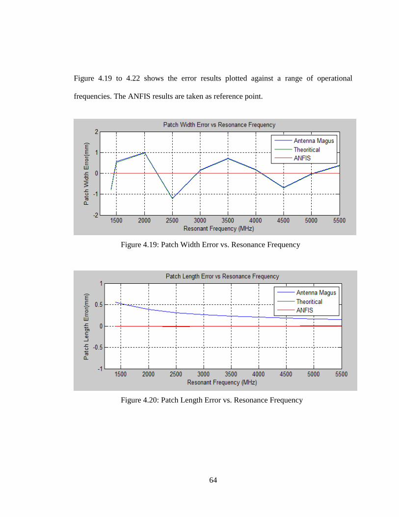
64
Figure 4.19 to 4.22 shows the error results plotted against a range of operational
frequencies. The ANFIS results are taken as reference point.
Figure 4.19: Patch Width Error vs. Resonance Frequency
Figure 4.20: Patch Length Error vs. Resonance Frequency

65
Figure 4.21: Feed Point along Patch Width Error vs. Resonance Frequency
Figure 4.22: Feed Point along Patch Length Error vs. Resonance Frequency
The simulations were carried out on the same computer so as to be able to monitor the
time taken by each software to complete the respective simulations. Running an ANFIS
simulation on MALTAB® took approximately 6 minutes. On the other hand, simulation
using Ansoft HFSS software took approximately 28 minutes to complete the modeling. It
can therefore, be seen that simulating antenna using Ansoft HFSS takes a longer time as
compared to ANFIS simulation. A complete computer usage time profile summary is
shown in Appendix D.

66
4.2.2. Experimental Results
Practical implementation of the simulated data was carried out so as to validate the ANFIS
model. Figure 4.23 shows a block diagram of the experimental setup used in testing the
patch antenna. Figure 4.24 and 4.25 shows fabricated antenna and practical setup of patch
antennas in the laboratory respectively.
SIGNAL
GENERATOR
RECEIVER
UNIT
COMPUTER
TRANSMITTING
ANTENNA
RECEIVING
ANTENNA
MODULATING
SIGNAL
Figure 4.23: Block Diagram of Experiment Setup
Figure 4.24: Fabricated Rectangular MPA

67
Figure 4.25: Experimentation Setup
ED-3200 Antenna Trainer Kit was used in practically testing the performance of
microstrip patch antenna in their far field. Antenna kit enables tests at frequencies of
500MHz, 2GHz, and 10GHz. As shown in Figure 4.25, two sets of patch antennas were
tested and mapped together. The first patch (patch1) was fabricated based on Antenna
Magus simulated data while the second patch (patch 2) was fabricated based on ANFIS
simulated data as seen in Figure 4.26. The antenna trainer kit signal generator connects
both the transmitter and receiver units as seen in Figure 4.23. It provides transmission
signal to the transmitter and a modulating signal to the receiver. The receiver unit then
rotates in a clockwise direction through a 360o angle. This rotation allows plotting of a
radiation pattern as seen in Figure 4.26.

68
Figure 4.26: Rectangular MPA Radiation Pattern
Figure 4.26 shows the E-Plane electric field radiation pattern indicating the radiation
intensity in dB. It was observed that ANFIS model produced slightly improved radiation
intensity of -0.2dB with the radiation intensity of -4.1dB as compared to results from
Antenna Magus simulated practical data which had a radiation intensity of -4.3dB. This
shows that based on validation with Antenna Magus software, ANFIS can be effectively
used to design MPAs. From the experimental set up, it was noted that the gain was lower
than the expected. This is because the set up was carried out in an open area (laboratory),
thus, other external factors (including reflections) affected the strength of signal. Also,
soldering the coaxial cable onto the antenna might have led to emission of spurious
radiation by the antenna.

69
CHAPTER FIVE
5.0. CONCLUSION AND RECOMMENDATION
5.1. Conclusion
In this thesis, a rectangular microstrip patch antenna has been successfully designed using
adaptive neuro-fuzzy inference optimization technique. The microstrip antenna designed
is completely planar in nature and does not have any cross-layered structures as have been
proposed elsewhere for bandwidth, gain, and radiation efficiency enhancement. The
proposed antenna was designed to operate at 2.0±5%GHz.
From the simulation results, it was observed that the formulated ANFIS model produces
results which are in agreement with simulated data from Antenna Magus software. The
main parameters that influence the antenna design are the dielectric constant of the
dielectric substrate, the feed location, patch length, and patch width.
A comparison of the ANFIS model simulation with the Antenna Magus simulation and
the theoretical results shows that there is a minimal difference of about 3% in the patch
dimensions with ANFIS model producing an improved simulated gain. Simulating an
antenna using HFSS took a significant time (about twenty eight minutes) with incidences
of memory overload. These simulations were carried out on a computer with a processor
of 2.2GHz core2duo and RAM of 2GB. Simulation using ANFIS took a significantly less
time (6 minutes) as compared to HFSS (28 minutes) thus has the advantage of less
computer time and memory usage. This demonstrates that ANFIS being fast and accurate

70
design methodology can be used to effectively design MPAs with complex structures and
other related work.
The overall performance of the prototype and the design goals were achieved. It was also,
observed that ANFIS can work hand in hand with another antenna design software so as
to plot various antenna characteristics.
5.2. Recommendation
The optimization routine of an antenna by ANFIS has a primary goal of minimizing the
design error as well as maximizing the antenna gain. Future work could focus on further
improving the ANFIS design methodology by formulating it to display various antenna
radiation characteristics.
When using commercial antenna design softwares to design antennas, convergence may
prove to be a challenge in the absence of a powerful central processing unit when
simulating structures with multiple layers. ANFIS can be used to aid in this design by
formulating a model that incorporates various types of multilayered antennas since ANFIS
model implemented in MATLAB® platform takes less computer memory and time to
optimize antenna parameters.
In this thesis, the rectangular patch antenna with only one specific band of frequencies
was considered. Patch antennas with multiband Frequencies can be designed using ANFIS
simulations.

71
REFERENCES
[1]. W. Stuart, ‘’Fundamentals of Electromagnetics with Engineering Applications’’,
John Wiley & Sons, NJ, USA, pp. 442‐445, 2005
[2]. K. Guney and N. Sarikaya, “Adaptive neuro-fuzzy inference system for computing
the resonant frequency of circular microstrip antennas”, Aces Journal, Vol. 19,
No. 3, pp. 188-197, November 2004
[3]. Chang Kai, “RF and Microwave Wireless Systems”, John Wiley & Sons, Inc.,
New York, pp. 90-98, 2000
[4]. Er Nitin Agarwal, Dr. D.C.Dhubkarya, Er Rinkesh Mittal, “Designing & Testing
of Rectangular Micro strip antenna operating at 2.0 GHz using IE3D”, Global
Journal of Researches in Engineering, Vol. 11, No. 1, pp. 44-48, February 2011
[5]. Deschamps, G.A., “Microstrip Microwave Antennas”, 3rd USAF Sysmp.
Antennas, University of Illinois, Urbana, 1953.
[6]. Gutton, H., and G. Baussinot, “Flat Aerial for Ultra High Frequencies,” French
Patent No. 703113, 1955.
[7]. Sainati, Robert A., “CAD of Microstrip Antennas for Wireless Applications”,
The Artec House Antenna Library, pp 1-18, January 1996
[8]. Balanis, Contantine A., “Antenna Theory – Analysis and Design”, 2nd Edition,
John Wiley & Sons Inc., pp. 722-751, 1997
[9]. K. Guney, and N. Sarikaya, “Comparison of adaptive-network-based fuzzy
inference systems for bandwidth calculation of rectangular microstrip antennas”,
Expert Systems with Applications 36, Elsevier Ltd., pp. 3522–3535, 2009.

72
[10]. K. Guney, and N. Sarikaya, “Adaptive Neuro-Fuzzy Inference Systems for
Computation of the Bandwidth of Electrically Thin and Thick Rectangular
Microstrip Antennas”, Electrical Engineering Journal 88, ©Springler-Verlag, pp.
201–210, 2006
[11]. Marine Corps, “Field Antenna Handbook”, Navy Department, Headquarters
United States Marine Corps Washington, D.C., pp. 48-51, 1999.
[12]. Dafalla, Z. 1., Kuan, W. T. Y., Abdel Rahman, A. M., and Shudakar, S. C.:
“Design of a Rectangular Microstrip Patch Antenna at 1 GHz.” RF and
Microwave Conference, Subang, Selangor, Malaysia, October 2004
[13]. Mehmet Kara, “Design Considerations for Rectangular Microstrip Antenna
Elements with Various Substrate Thicknesses”, Microwave and Optical
Technology Letters / Vol. 19, No. 2, pp. 111-121, October 1998.
[14]. Saeed, A. Rashid and Khatum, Sabira, “Design of Microstrip Antenna for
WLAN”, Journal of Applied Sciences 5 (1), ©Asian Network for Scientific
Information, pp. 47-51, 2005
[15]. Bratislav Milovanovic, Marija Milijic, Aleksandar Atanaskovic, and Zoran
Stankovic, “Modeling of Patch Antennas using Neural Networks”, Telskiks,
Serbia and Montenegro, ©IEEE, 2005
[16]. Indrasen Singh et al, “Microstrip Patch Antenna and its Applications: a Survey”,
Int. J. Comp. Tech. Appl., Vol. 2, pp. 1595-1599, 2011

73
[17]. Papi, D. G., “An Artificial Intelligence Applications for Architectural Textures
Analysis”, The International Archives of the Photogrammetry, Remote Sensing
and Spatial Information Sciences, Vol. XXXIV, Part 5/W12, 2003
[18]. Jang and Gulley, ‘MATLAB Fuzzy Logic Toolbox’, The MathWorks, Inc., pp.
16-41, 84-93, 1997
[19]. Lofti A. Zadeh, ‘Fuzzy Logic – Computing with Words’, IEEE Transactions on
Fuzzy Systems, Vol. 4, No. 2, pp. 103-111, May 1996
[20]. S. N. Sivanandam, S. Sumathi and S. N. Deepa, “Introduction to Fuzzy Logic
using MATLAB”, Springer-Verlag Berlin Heidelberg, pp. 10-127, 2007
[21]. Ben Krose and Patric Van Der Smagt, “An Introduction to Neural Networks”, 8th
Edition, University of Amsterdam, pp. 1-45, 1996.
[22]. Kasabov, K. Nikola, “Foundations of Neural Networks, Fuzzy Systems, and
Knowledge Engineering”, The MIT Press Cambridge, Massachusetts London,
England, pp. 1-19, 167-329, 1998
[23]. Robert Fuller, “Neural Fuzzy Systems”, Abo Akademi University, ISBN 951-
650-624-0, 1995
[24]. Jang et.al, “Neuro-Fuzzy and Soft Computing”, Prentice Hall Upper Saddle
River, pp. 1-42, 197-223, 333-360, 1997
[25]. Ariffin, Kasuma Bin, “On Neuro-Fuzzy Applications for Automatic Control,
Supervision, and Fault Diagnosis for Water Treatment Plant”, A Thesis
submitted to the Faculty of Electrical Engineering, Universiti Teknologi,
Malaysia, 2007.

74
[26]. K. Guney, and N. Sarikaya, “Adaptive Neuro-Fuzzy Inference System for
Computing Patch Radius of Circular Microstrip Antennas”, Microwave and
Optical Technology Letters, Vol. 48, No. 8, pp. 1606–1610, Feb. 2007
[27]. N. Sarikaya, K. Guney, and C. Yildiz, “Adaptive Neuro-Fuzzy Inference System
for the Computational of the Characteristic Impedance and the Effective
Permittivity of the Micro-Planar Strip Line”, Faculty of Engineering, Erciyes
University, Kayseri, ©IEEE, 2005
[28]. Zoltan Himer, et.al, “Control of Combustion Base on Neuro-Fuzzy Model”,
Systems Engineering Laboratory, University of Oulu, Finland, 2006
[29]. Jang, Roger, “ANFIS: Adaptive-Network-Based Fuzzy Inference System”, IEEE
Transactions on Systems, MAN, and Cybernetics, Vol. 23, No. 3, pp. 665-685,
1993
[30]. Kapil Goswami et.al, “Design and Analysis of Rectangular Microstrip Antenna
with PBG Structure for Enhancement of Bandwidth”, Global Journal of Research
Engineering, Vol. 11, Issue 2, Version 1.0, pp. 22-28, March 2011
[31]. A. Hameed and B. Khalaf, “Design and Simulation of Broadband Rectangular
Microstrip Antenna”, Eng. Tech., Vol. 26, No. 1, pp. 93-121, 2008
[32]. Vivekananda L. Subrahmanya, “Pattern Analysis of Rectangular Microstrip
Patch Antenna”, A Thesis submitted to the School of Engineering, University
College of Boras, Boras, 2009.
[33]. N. Turker, et.al, “Artificial Neural Design of Microstrip Antennas” , Turk J Elec.
Engin., Vol. 14, No. 3, pp. 4 45-453, 2006

75
[34]. K. Guney, “Simple and Accurate Formulas for the Physical Dimensions of
Rectangular Microstrip Antennas with Thin and Thick Substrates”, Microwave
and Optical Technology Letters, Vol. 44, No. 3, pp. 257-259, February 2005
[35]. A.B. Mutiara, R. Refianti, and Rachmansyah, “Design of Microstrip Antenna for
Wireless Communication at 2.4GHz”, Journal of Theoretical and Applied
Information Technology, Vol. 33, No. 2, pp. 184-192, November 2011
[36]. V.V. Thakare and Singhal, “Analysis of Feed Point Coordinates of a Coaxial
Feed Rectangular Microstrip Antenna using Mlpffbp Artificial Neural Network”,
ICIT 5th International Conference on Information Technology, pp. 1-6, 2011
[37]. Ali Dheyab and Karim Hamad, “ Improving Bandwidth of Rectangular Patch
Antenna using Different Thickness of Dielectric Substrate” , ARPN Journal of
Engineering and Applied Sciences, Vol. 6, No. 4, pp. 16-21, April 2011
[38]. John Ojha and Marc Peters, “Microwave and Millimeter Wave Technologies –
Modern UWB Antennas and Equipment”, In Tech Publishers, Europe, ISBN
978-953-7619-67-1, March 2010.

76
APPENDICES
APPENDIX A: MATLAB® PROGRAM CODE
APPENDIX A-1: Training Data Sets Generation MATLAB® Program Code
function final = antennaparameters
v = 3e8; %Speed of Light (m/s) c = v; %Speed of Light (m/s) fo_in = input(' Please enter the Resonant Frequency = ' ) fo = [fo_in (1.5e9:500e6:8e9)]; %Resonant Frequency Erin = input(' Please enter the Dielectric constant = ' ) hin = input(' Please enter the substrate thickness in Metres = ' ) wavelenght = c./fo; %Calculates the Wavelength. Erd = 2.2; %Dielectric Constant of the Duroid 5880 Substrate hd = 0.00157; %Height of the Duroid 5880 Substrate in Metres Erg = 4.35; %Dielectric Constant of the FR4 Glass Epoxy Substrate hg = 0.0016; %Height of the FR4 Glass Epoxy Substrate in Metres Eru = 10; %Dielectric Constant of DiClad880 Substrate hu = 0.0022;%Height of DiClad880 Substrate in Metres Ers = 11.9; %Dielectric Constant of a Silicon Substrate hs = 0.0015; %Height of Silicon Substrate in Metres Era = 9.8; %Dielectric Constant of Alumina Substrate ha = 0.0015; %Height of Alumina Substrate in Metres
%----------------------------------------------------------------------
----
%The Patch Width (W)
Wd = v./(2.*fo)*sqrt(2/(Erd+1)); %Width of Duroid 5880 Substrate in
(M) Wdmm = 1000.*Wd; %Patch Width of Duroid 5880 Substrate in mm
Wg = v./(2.*fo)*sqrt(2/(Erg+1)); %Width of FR4 Glass Epoxy
Substrate(M) Wgmm = 1000.*Wg; %Patch Width of FR4 Glass Epoxy Substrate in
mm
Wu = v./(2.*fo)*sqrt(2/(Eru+1)); %Patch Width of DiClad880
Substrate (M) Wumm = 1000.*Wu; %Patch Width of DiClad880 Substrate in mm

77
Ws = v./(2.*fo)*sqrt(2/(Ers+1)); %Patch Width of Silicon Substrate
(M) Wsmm = 1000.*Ws; %Patch Width of Silicon Substrate in mm
Wa = v./(2.*fo)*sqrt(2/(Era+1)); %Patch Width of Alumina Substrate
(M) Wamm = 1000.*Wa; %Patch Width of Alumina Substrate in mm
%----------------------------------------------------------------------
----
%Effective Dielectric Constant (Ereff)
Ereffd = ((Erd+1)/2)+((Erd-1)/2)*(1./sqrt(1+(hd.*12./Wd))); %Effective Dielectric Constant (Ereff) of Duroid 5880 Substrate
Ereffg = ((Erg+1)/2)+((Erg-1)/2)*(1./sqrt(1+(hg.*12./Wg))); %Effective Dielectric Constant (Ereff) of FR4 Glass Epoxy Substrate
Ereffu = ((Eru+1)/2)+((Eru-1)/2)*(1./sqrt(1+(hu.*12./Wu))); %Effective Dielectric Constant (Ereff) of DiClad880 Substrate
Ereffs = ((Ers+1)/2)+((Ers-1)/2)*(1./sqrt(1+(hs.*12./Ws))); %Effective Dielectric Constant (Ereff) of Silicon Substrate
Ereffa = ((Era+1)/2)+((Era-1)/2)*(1./sqrt(1+(ha.*12./Wa))); %Effective Dielectric Constant (Ereff) of Alumina Substrate
%----------------------------------------------------------------------
----
%Effective Length (Leff)
%Calculates the Effective Length for the corresponding Effective %Dielectric constant in metres respectively.
Leffd = c./(2.*fo.*sqrt(Ereffd));
Leffg = c./(2.*fo.*sqrt(Ereffg));
Leffu = c./(2.*fo.*sqrt(Ereffu));
Leffs = c./(2.*fo.*sqrt(Ereffs));
Leffa = c./(2.*fo.*sqrt(Ereffa));
%----------------------------------------------------------------------
----

78
%Length Extension (Lextn)
%Calculates the Length Extension in metres respectively
Lextnd = (0.412*hd).*(((Ereffd+0.3).*(Wd./hd+0.264))./((Ereffd-... 0.258).*(Wd./hd+0.8)));
Lextng = (0.412*hg).*(((Ereffg+0.3).*(Wg./hg+0.264))./((Ereffg-... 0.258).*(Wg./hg+0.8)));
Lextnu = (0.412*hu).*(((Ereffu+0.3).*(Wu./hu+0.264))./((Ereffu-... 0.258).*(Wu./hu+0.8)));
Lextns = (0.412*hs).*(((Ereffs+0.3).*(Ws./hs+0.264))./((Ereffs-... 0.258).*(Ws./hs+0.8)));
Lextna = (0.412*ha).*(((Ereffa+0.3).*(Wa./ha+0.264))./((Ereffa-... 0.258).*(Wa./ha+0.8)));
%----------------------------------------------------------------------
----
%Patch Length (L (mm))
Ld = Leffd - 2.*Lextnd; Ldmm = 1000*Ld; %Patch Length of Duroid 5880 Substrate in mm
Lg = Leffg - 2.*Lextng; Lgmm = 1000*Lg; %Patch Length in of FR4 Glass Epoxy Substrate
mm
Lu = Leffu - 2.*Lextnu; Lumm = 1000*Lu; %Patch Length of DiClad880 Substrate in mm
Ls = Leffs - 2.*Lextns; Lsmm = 1000*Ls; %Patch Length of Silicon Substrate in mm
La = Leffa - 2.*Lextna; Lamm = 1000*La; %Patch Length of Alumina Substrate in mm
%----------------------------------------------------------------------
----
%Bandwidth (BW)
BWd = 3.77*(((Erd-1)./Erd^2).*(Wd./Ld).*(hd./wavelenght)); BWdp = 100.*BWd; %BW of Duroid 5880 Substrate in percentage

79
BWg = 3.77*(((Erg-1)./Erg^2).*(Wg./Lg).*(hg./wavelenght)); BWgp = 100.*BWg; %BW of FR4 Glass Epoxy Substrate in
percentage
BWu = 3.77*(((Eru-1)./Eru^2).*(Wu./Lu).*(hu./wavelenght)); BWup = 100.*BWu; %BW of Didad880 Substrate in percentage
BWs = 3.77*(((Ers-1)./Ers^2).*(Ws./Ls).*(hs./wavelenght)); BWsp = 100.*BWs; %BW of Silicon Substrate in percentage
BWa = 3.77*(((Era-1)./Era^2).*(Wa./La).*(ha./wavelenght)); BWap = 100.*BWa; %BW of Alumina Substrate in percentage
%----------------------------------------------------------------------
----
%Feed Co-ordinates
%Feed Co-ordinates of Duroid 5880 Substrate Yfd = Wd./2; %Feed point along the Patch Width. Yfdmm = 1000.*Yfd; %Feed point along the Patch Width in mm. Xfd = Ld./(2.*sqrt(Ereffd)); %Feed Point along the Patch Legth. Xfdmm = 1000.*Xfd; %Feed Point along the Patch Legthin mm.
%Feed Co-ordinates of FR4 Glass Epoxy Substrate Yfg = Wg./2; %Feed point along the Patch Width. Yfgmm = 1000.*Yfg; %Feed point along the Patch Width in mm. Xfg = Lg./(2.*sqrt(Ereffg)); %Feed Point along the Patch Legth. Xfgmm = 1000.*Xfg; %Feed Point along the Patch Legthin mm.
%Feed Co-ordinates of Didad880 Substrate Yfu = Wu./2; %Feed point along the Patch Width. Yfumm = 1000.*Yfu; %Feed point along the Patch Width in mm. Xfu = Ld./(2.*sqrt(Ereffu)); %Feed Point along the Patch Legth. Xfumm = 1000.*Xfu; %Feed Point along the Patch Legthin mm.
%Feed Co-ordinates of Silicon Substrate Yfs = Ws./2; %Feed point along the Patch Width. Yfsmm = 1000.*Yfs; %Feed point along the Patch Width in mm. Xfs = Ls./(2.*sqrt(Ereffs)); %Feed Point along the Patch Legth. Xfsmm = 1000.*Xfs; %Feed Point along the Patch Legthin mm.
%Feed Co-ordinates of Alumina Substrate Yfa = Wa./2; %Feed point along the Patch Width. Yfamm = 1000.*Yfa; %Feed point along the Patch Width in mm. Xfa = La./(2.*sqrt(Ereffa)); %Feed Point along the Patch Legth. Xfamm = 1000.*Xfa; %Feed Point along the Patch Legthin mm.
%----------------------------------------------------------------------
----

80
%Plane Ground Dimensions
%Plane Ground Dimensions of Duroid 5880 Substrate Lgd = 1000*((6*hd)+Ld); %Plane Ground Dimension along the Lenght. Wgd = 1000*((6*hd)+Wd); %Plane Ground Dimension along the Width.
%Plane Ground Dimensions of FR4 Glass Epoxy Substrate Lgg = 1000*((6*hg)+Lg); %Plane Ground Dimension along the Lenght. Wgg = 1000*((6*hg)+Wg); %Plane Ground Dimension along the Width.
%Plane Ground Dimensions of Didad880 Substrate Lgu = 1000*((6*hu)+Lu); %Plane Ground Dimension along the Lenght. Wgu = 1000*((6*hu)+Wu); %Plane Ground Dimension along the Width.
%Plane Ground Dimensions of Silicon Substrate Lgs = 1000*((6*hs)+Ls); %Plane Ground Dimension along the Lenght. Wgs = 1000*((6*hs)+Ws); %Plane Ground Dimension along the Width.
%Plane Ground Dimensions of Alumina Substrate Lga = 1000*((6*ha)+La); %Plane Ground Dimension along the Lenght. Wga = 1000*((6*ha)+Wa); %Plane Ground Dimension along the Width.
%----------------------------------------------------------------------
----
%Calculations for the patch material being experimented. %Specific input figures are got from an interactive Matlab
workspace.
Win = v./(2*fo).*sqrt(2/(Erin+1)); %Patch Width in Metres Winmm = 1000*Win; %Patch Width of Substrate material (mm)
Ereffin = ((Erin+1)/2)+((Erin-
1)/2)*(1./sqrt(1+(hin.*12./Win))); %Effective Dielectric Constant (Ereff)
Leffin = c./(2.*fo.*sqrt(Ereffin)); %Effective Length Lextnin = (0.412*hin).*(((Ereffin+0.3).*(Win./hin+... 0.264))./((Ereffin-0.258).*(Win./hin+0.8))); %Calculates the Length Extension in metres respectively
Lin = Leffin - 2.*Lextnin; Linmm = 1000*Lin; %Patch Length in mm
BWin = 3.77*(((Erin-
1)./Erin^2).*(Win./Lin).*(hin./wavelenght)); BWinp = 100.*BWin; %BW of in percentage
WLdin = c./(fo.*sqrt(Erin));%Wavelength of Dielectric Substrate

81
haWLdin = (hin./WLdin).*1000;
%Feed Co-ordinates of a Substrate Yfin = Win./2; %Feed point along the Patch Width. Yfinmm = 1000.*Yfin; %Feed point along the Patch Width in mm. Xfin = Lin./(2.*sqrt(Ereffin)); %Feed Point along the Patch
Legth. Xfinmm = 1000.*Xfin; %Feed Point along the Patch Legthin mm.
%Plane Ground Dimensions of a Substrate Lgin = 1000*((6*hin)+Lin); %Plane Ground Dimension along the
Lenght Wgin = 1000*((6*hin)+Win); %Plane Ground Dimension along the
Width.
%----------------------------------------------------------------------
----
%Arranging the Dielectric Constants of various materials and their %respective Substrate Dielectric Heights into columns. n = ones(1,15); z1 = Erd*n; z2 = Erg*n; z3 = Eru*n; z4 = Ers*n; z5 = Era*n; zin = Erin*n;
y1 = hd*n*1000; y2 = hg*n*1000; y3 = hu*n*1000; y4 = hs*n*1000; y5 = ha*n*1000; yin = hin*n*1000;
%----------------------------------------------------------------------
---- %Converting the Resonant Frequency to MHz
fo2 = fo./1e6;
%----------------------------------------------------------------------
----
%The simulation results are then re-arranged to be used as data set in %ANFIS training as follows;
%First, the columns to be used for optimization are arranged as per the %columns as follows where, %Column 1 - Resonant Frequency, Column 2 - Dielectric Constants, Column
3 -

82
%Dielectric Substrate Heights, Column 4 - Patch Width, Column 5 - Patch %Length, Column 6a - Feed Point along the Patch Width, Column 6b - Feed %Point along the Patch Length.
trncolumn1 = [fo2';fo2';fo2';fo2';fo2';fo2']; trncolumn2 = [z1';z2';z3';z4';z5';zin']; trncolumn3 = [y1';y2';y3';y4';y5';yin']; trnset1 = [trncolumn1 trncolumn2 trncolumn3]; save trnset1
trncolumn4 = [Wdmm';Wgmm';Wumm';Wsmm';Wamm';Winmm']; save trncolumn4
trncolumn5 = [Ldmm';Lgmm';Lumm';Lsmm';Lamm';Linmm']; save trncolumn5
trncolumn6a = [Yfdmm';Yfgmm';Yfumm';Yfsmm';Yfamm';Yfinmm']; save trncolumn6a
trncolumn6b = [Xfdmm';Xfgmm';Xfumm';Xfsmm';Xfamm';Xfinmm']; save trncolumn6b
Lgall = [Lgd';Lgg';Lgu';Lgs';Lga';Lgin']; Wgall = [Wgd';Wgg';Wgu';Wgs';Wga';Wgin']; BWall = [BWdp';BWgp';BWup';BWsp';BWap';BWinp'];
final = [trnset1 trncolumn4 trncolumn5 trncolumn6a trncolumn6b... Lgall Wgall BWall]; save final end

83
APPENDIX A-2: Testing Data Sets MATLAB® Program Code
%In this page, the testing/checking data used in ANFIS optimization is %listed below;
%----------------------------------------------------------------------
---- %First, the data used in the first phase comprising of Frequency, %Dielectric Constant, Height of Substrate and Patch Width are listed as %shown below %----------------------------------------------------------------------
----
% Frequency Er Height Width % GHz (mm) (mm) chkcolumn1 = [2310 2.33 3.175 57;... 4805 2.33 1.57 18.1;... 8000 3.78 1.7 12.13;... 2000 4.3 1.6 46.07;... 3000 10 2.2 21.32;... 5600 2.33 0.254 20.76;... 5820 2.55 4.76 10.00;... 3200 2.55 12.81 10.30;... 3580 2.55 9.52 12.56;... 2200 2.5 1.524 68.58;... 5100 2.55 4.76 13.75;... 1500 11.9 1.5 39.375;... 2000 4.3 1.6 46.072;... 3500 2.45 0.483 32.631;... 3500 9.8 1.5 18.443;... 5000 11.9 1.5 11.813;... 7500 4.3 1.5 12.286;... 5060 2.33 1.57 17.2];
save chkcolumn1
%----------------------------------------------------------------------
---- %Secondly, the data used in the second phase comprising of Frequency, %Dielectric Constant, Height of Substrate and Patch Width, and Patch %Length are listed as shown below %----------------------------------------------------------------------
----
% Frequency Er Height Width Length % GHz (mm) (mm) (mm) chkcolumn2 = [2310 2.33 3.175 57 38.00;... 4805 2.33 1.57 18.1 19.60;... 8000 3.78 1.7 12.13 6.885;... 5600 10.20 1.27 10.00 9.10;...

84
5820 2.55 4.76 10.00 15.20;... 3200 2.55 12.81 10.30 33.80;... 3580 2.55 9.52 12.56 27.56;... 2200 2.5 1.524 68.58 41.40;... 5100 2.55 4.76 13.75 15.80;... 1500 11.9 1.5 39.375 28.925;... 2000 4.3 1.6 46.072 35.846;... 3500 2.45 0.483 32.631 27.206;... 3500 9.8 1.5 18.443 13.409;... 5000 11.9 1.5 11.813 8.317;... 7500 4.3 1.5 12.286 9.046;... 5060 2.33 1.57 17.2 18.60];
save chkcolumn2
%----------------------------------------------------------------------
---- %Also, the data used in the third phase comprising of Frequency, %Dielectric Constant, Height of Substrate and Patch Width, Patch
Length, %and Feed Point (Yf) along the Patch Width are listed as shown below %----------------------------------------------------------------------
----
% Frequency Width Length Feed Point % GHz (mm) (mm) Yf(mm) chkcolumn3 = [2440 29.22 24.33 16.56;... 1700 34.12 23.66 22.71;... 8000 12.13 6.885 2.40;... 2000 30.22 23.60 17.36;... 1910 30.45 24.11 18.575;... 2400 62.04 46.23 20.0;... 2450 37.86 29.66 7.52;... 1912 31.1 22.80 0.0;... 2290 29.77 22.10 22.635;... 1500 11.9 1.5 19.688;... 2000 4.3 1.6 23.036;... 3500 2.45 0.483 16.315;... 3500 9.8 1.5 9.221;... 5000 11.9 1.5 5.906;... 7500 4.3 1.5 6.143];
save chkcolumn3
%----------------------------------------------------------------------
---- %Finally, the data used in the fourth phase comprising of Frequency, %Dielectric Constant, Height of Substrate and Patch Width, Patch
Lenght, %and Feed Point (Xf) along the Patch Length are listed as shown below %----------------------------------------------------------------------
----

85
% Frequency Width Length Feed Point % GHz (mm) (mm) Xf(mm) chkcolumn4 = [2440 29.22 24.33 17.115;... 1700 34.12 23.66 15.38;... 8000 12.13 6.885 6.065;... 2000 30.22 23.60 14.05;... 1910 30.45 24.11 21.305;... 2400 62.04 46.23 11.0 ;... 2450 37.86 29.66 18.78;... 1912 31.1 22.80 4.0;... 2290 29.77 22.10 17.5;... 1500 11.9 1.5 4.368;... 2000 4.3 1.6 8.921;... 3500 2.45 0.483 9.069;... 3500 9.8 1.5 2.296;... 5000 11.9 1.5 1.323;... 7500 4.3 1.5 2.351]; save chkcolumn4

86
APPENDIX A-3: ANFIS MATLAB® Program Code
This program aims at optimizing the parameters used in the design of a %rectangular microstrip patch antenna by using adaptive neuro-fuzzy %inference system technique.
clear all run antennaparameters run antennachkdata
%----------------------------------------------------------------------
---- %On the First Phase, the Patch Width is optimized based on three
parameters %(Resonant Frequency, Dielectric Constant, & Substrate Height) as
follows;
'OPTIMIZATION OF ANTENNA PATCH WIDTH USING ANFIS' %----------------------------------------------------------------------
---- %This loads both the training and checking data used by ANFIS.
load trnset1.mat load trncolumn4.mat load chkcolumn1.mat load final.mat
%----------------------------------------------------------------------
----
trnData1 = [trnset1 trncolumn4]; chkData1 = chkcolumn1;
numMFs = [4 3 3]; mfType = 'gbellmf'; fismat = genfis1(trnData1,numMFs,mfType);
showfis(fismat) showrule(fismat) ruleview(fismat) ruleedit(fismat)
fismat = setfis(fismat, 'name','PATCH WIDTH'); fismat = setfis(fismat, 'input',1,'name','Resonant Frequency'); fismat = setfis(fismat, 'input',2,'name','Dielectric
Constant'); fismat = setfis(fismat, 'input',3,'name','Substrate Height'); fismat = setfis(fismat, 'output',1,'name','Patch Width');

87
figure (1); plotfis(fismat);
figure (2); for input_index=1:3, subplot(2,2,input_index) [x,y]=plotmf(fismat,'input',input_index) ; plot(x,y) axis([-inf inf 0 1.2]); xlabel(['Input ' int2str(input_index)]); title('Initial Membership Values') end
numEpochs = 700;
[fismat1,trnErr,ss1,fismat2,chkErr] = anfis(trnData1,fismat,... [numEpochs 0 0.04 0.9 1.1],NaN,chkData1,1);
trnOut = evalfis([trnData1(:,1) trnData1(:,2)
trnData1(:,3)],fismat1); trnRMSE1 = norm(trnOut - trnData1(:,4))/sqrt(length(trnOut));
epoch = 1:numEpochs;
figure (3); plot(epoch,trnErr,'o',epoch,chkErr,'x') hold on; plot(epoch,[trnErr chkErr]); hold off
trndW = evalfis([trnData1(:,1) trnData1(:,2)
trnData1(:,3)],fismat1);
' Please Press ENTER Key to Continue' pause
%----------------------------------------------------------------------
---- %On Second Phase, the Patch Length is optimized based on four
parameters %(Resonant Frequency, Dielectric Constant, Optimized Width, & Substrate %Height) as follows;
'OPTIMIZATION OF ANTENNA PATCH LENGTH USING ANFIS' %----------------------------------------------------------------------
----
load trncolumn5.mat load chkcolumn2.mat

88
%----------------------------------------------------------------------
----
trnData2 = [trnset1 trndW trncolumn5]; chkData2 = chkcolumn2;
numMFs = [4 2 2 4]; mfType = 'gbellmf'; fismat_2 = genfis1(trnData2,numMFs,mfType);
showfis(fismat_2) showrule(fismat_2) ruleview(fismat_2) ruleedit(fismat_2) fismat_2 = setfis(fismat_2,'name','PATCH LENGTH'); fismat_2 = setfis(fismat_2,'input',1,'name','Resonant
Frequency'); fismat_2 = setfis(fismat_2,'input',2,'name','Dielectric
Constant'); fismat_2 = setfis(fismat_2,'input',3,'name','Substrate
Height'); fismat_2 = setfis(fismat_2,'input',4,'name','Optimized Width'); fismat_2 = setfis(fismat_2,'output',1,'name','Patch Length');
figure (4); plotfis(fismat_2)
figure (5); for input_index=1:4, subplot(2,2,input_index) [x,y]=plotmf(fismat_2,'input',input_index); plot(x,y) axis([-inf inf 0 1.2]); xlabel(['Input ' int2str(input_index)]); title('Initial Membership Values') end
numEpochs = 600;
[fismat3,trnErr2,ss2,fismat4,chkErr2] = anfis(trnData2,fismat_2,... [numEpochs 0 0.04 0.9 1.1],NaN,chkData2,1);
trnOut2 = evalfis([trnData2(:,1) trnData2(:,2) trnData2(:,3)... trnData2(:,4)],fismat3); trnRMSE2 = norm(trnOut2 - trnData2(:,5))/sqrt(length(trnOut2));
epoch = 1:numEpochs;
figure (6);

89
plot(epoch,trnErr2,'o',epoch,chkErr2,'x') hold on; plot(epoch,[trnErr2 chkErr2]); hold off
trndL = evalfis([trnData2(:,1) trnData2(:,2) trnData2(:,3)... trnData2(:,4)],fismat3);
' Please Press ENTER Key to Continue' pause
%----------------------------------------------------------------------
---- %On the Third Phase, the Antenna Feed Point (Yf) is optimized based on %Five parameters(Resonant Frequency, Dielectric Constant, Substrate %Height, Optimized Width, & Optimized Length) as follows;
'OPTIMIZATION OF ANTENNA FEED POINT (Yf) USING ANFIS' %----------------------------------------------------------------------
----
load trncolumn6a.mat load chkcolumn3.mat %----------------------------------------------------------------------
---- trnData3 = [trncolumn1 trndW trndL trncolumn6a]; chkData3 = chkcolumn3; numMFs = [3 4 4]; mfType 'gbellmf'; fismat_3 = genfis1(trnData3,numMFs,mfType);
showfis(fismat_3) showrule(fismat_3) ruleview(fismat_3) ruleedit(fismat_3)
fismat_3 = setfis(fismat_3,'name','FEED POINT Yf'); fismat_3 = setfis(fismat_3,'input',1,'name','Resonant
Frequency'); fismat_3 = setfis(fismat_3,'input',2,'name','Optimized Width'); fismat_3 = setfis(fismat_3,'input',3,'name','Optimized
Length'); fismat_3 = setfis(fismat_3,'output',1,'name','Feed Point Yf');
figure (7); plotfis(fismat_3)
figure (8); for input_index=1:3, subplot(2,2,input_index) [x,y]=plotmf(fismat_3,'input',input_index);

90
plot(x,y) axis([-inf inf 0 1.2]); xlabel(['Input ' int2str(input_index)]); title('Initial Membership Values') end
numEpochs = 600;
[fismat5,trnErr3,ss3,fismat6,chkErr3] = anfis(trnData3,fismat_3,... [numEpochs 0 0.04 0.9 1.1],NaN,chkData3,1);
trnOut3 = evalfis([trnData3(:,1) trnData3(:,2)
trnData3(:,3)],fismat5); trnRMSE3 = norm(trnOut3 - trnData3(:,4))/sqrt(length(trnOut3));
epoch3 = 1:numEpochs;
figure (9); plot(epoch3,trnErr3,'o',epoch3,chkErr3,'x') hold on; plot(epoch3,[trnErr3 chkErr3]); hold off
trndYf = evalfis([trnData3(:,1) trnData3(:,2)
trnData3(:,3)],fismat5);
' Please Press ENTER Key to Continue' pause
%----------------------------------------------------------------------
---- %On the Third Phase, the Antenna Feed Point (Xf) is optimized based on %Five parameters(Resonant Frequency, Dielectric Constant, Substrate %Height, Optimized Width, & Optimized Length) as follows;
'OPTIMIZATION OF ANTENNA FEED POINT (Xf) USING ANFIS' %----------------------------------------------------------------------
----
load trncolumn6b.mat load chkcolumn4.mat
%----------------------------------------------------------------------
----
trnData4 = [trncolumn1 trndW trndL trncolumn6b]; chkData4 = chkcolumn4;
numMFs = [3 4 4]; mfType = 'gbellmf';

91
fismat_4 = genfis1(trnData4,numMFs,mfType);
showfis(fismat_4) showrule(fismat_4) ruleview(fismat_4) ruleedit(fismat_4)
fismat_4 = setfis(fismat_4,'name','FEED POINT Xf'); fismat_4 = setfis(fismat_4,'input',1,'name','Resonant
Frequency'); fismat_4 = setfis(fismat_4,'input',2,'name','Optimized Width'); fismat_4 = setfis(fismat_4,'input',3,'name','Optimized
Length'); fismat_4 = setfis(fismat_4,'output',1,'name','Feed Point Xf');
figure (10); plotfis(fismat_4)
figure (11); for input_index=1:3, subplot(2,2,input_index) [x,y]=plotmf(fismat_4,'input',input_index); plot(x,y) axis([-inf inf 0 1.2]); xlabel(['Input ' int2str(input_index)]); title('Initial Membership Values') end
numEpochs = 600;
[fismat7,trnErr4,ss4,fismat8,chkErr4] = anfis(trnData4,fismat_4,... [numEpochs 0 0.04 0.9 1.1],NaN,chkData4,1);
trnOut4 = evalfis([trnData4(:,1) trnData4(:,2)
trnData4(:,3)],fismat7); trnRMSE4 = norm(trnOut4 - trnData4(:,4))/sqrt(length(trnOut4));
epoch4 = 1:numEpochs;
figure (12); plot(epoch4,trnErr4,'o',epoch4,chkErr4,'x') hold on; plot(epoch4,[trnErr4 chkErr4]); hold off
trndXf = evalfis([trnData4(:,1) trnData4(:,2)
trnData4(:,3)],fismat7);
' Please Press ENTER Key to Continue' pause

92
%----------------------------------------------------------------------
---- %The final optimized Antenna Design Parameters are listed in this
section %Also, in the same section, the final design parameter values are saved
as %an excel document under the Matlab Folder. Anytime the simulation is %carried out, the final values are then appended in the same file named %PATCHANTENNA.
'OVERALL OPTIMIZATION RESULTS' %----------------------------------------------------------------------
----
optmzdparameters = [trndW trndL trndYf trndXf] save optmzdparameters
allparameters = {'Fr' 'Er' 'h' 'optW' 'OptL' 'OptYf' 'OptXf' 'Lg'
'Wg';... trncolumn1 trncolumn2 trncolumn3 trndW trndL trndYf trndXf Lgall
Wgall};
allt = [trncolumn1 trncolumn2 trncolumn3 trndW trndL trndYf trndXf
Lgall... Wgall];
save allparameters
s = xlswrite('patchantenna.xls', allparameters, 'simulation',
'B1'); s2 = xlswrite('patchantenna.xls', allt, 'simulation', 'B3');
%----------------------------------------------------------------------
---- %Here, the graphs of relationship between frequency and Optimized Patch %Width, Patch Length, Feed Point along the Width Yf, and Feed Point
along %the Length Xf are plotted as shown below in figure 13 to 16.
fd = xlsread('patchantenna.xls', 'simulation', 'B3:B17'); fg = xlsread('patchantenna.xls', 'simulation', 'B18:B32'); fa = xlsread('patchantenna.xls', 'simulation', 'B63:B77'); fin = xlsread('patchantenna.xls', 'simulation', 'B78:B92');
Wd = xlsread('patchantenna.xls', 'simulation', 'E3:E17'); Wg = xlsread('patchantenna.xls', 'simulation', 'E18:E32'); Wa = xlsread('patchantenna.xls', 'simulation', 'E63:E77'); Win = xlsread('patchantenna.xls', 'simulation', 'E78:E92');
Ld = xlsread('patchantenna.xls', 'simulation', 'F3:F17'); Lg = xlsread('patchantenna.xls', 'simulation', 'F18:F32');

93
La = xlsread('patchantenna.xls', 'simulation', 'F63:F77'); Lin = xlsread('patchantenna.xls', 'simulation', 'F78:F92');
Yfd = xlsread('patchantenna.xls', 'simulation', 'G3:G17'); Yfg = xlsread('patchantenna.xls', 'simulation', 'G18:G32'); Yfa = xlsread('patchantenna.xls', 'simulation', 'G63:G77'); Yfin = xlsread('patchantenna.xls', 'simulation', 'G78:G92'); Xfd = xlsread('patchantenna.xls', 'simulation', 'H3:H17'); Xfg = xlsread('patchantenna.xls', 'simulation', 'H18:H32'); Xfa = xlsread('patchantenna.xls', 'simulation', 'H63:H77'); Xfin = xlsread('patchantenna.xls', 'simulation', 'H78:H92');
%Figure 13 plots Resonance Frequency vs Optimized Patch Width figure (13); plot (Wd,fd,Wg,fg,Wa,fa,Win,fin); axis([0 90 1000 8500]); legend('Er=2.2,h=1.57mm','Er=4.35,h=1.6mm','Er=9.8,h=1.5mm',... 'Er & h =Input') grid xlabel('Optimized Patch Width (mm)') ylabel('Resonant Frequency (MHz)') title('Patch Width vs Resonance Frequency')
%Figure 14 plots Resonance Frequency vs Optimized Patch Length figure (14); plot (Ld,fd,Lg,fg,La,fa,Lin,fin); axis([0 85 1000 8500]); legend('Er=2.2,h=1.57mm','Er=4.35,h=1.6mm','Er=9.8,h=1.5mm',... 'Er & h =Input') grid xlabel('Optimized Patch Length (mm)') ylabel('Resonant Frequency (MHz)') title('Patch Length vs Resonance Frequency')
%Figure 15 plots Resonance Frequency vs Optimized Feed Pont along the
Width figure (15); plot (Yfd,fd,Yfg,fg,Yfa,fa,Yfin,fin); axis([0 50 1000 8500]); legend('Er=2.2,h=1.57mm','Er=4.35,h=1.6mm','Er=9.8,h=1.5mm',... 'Er & h =Input') grid xlabel('Optimized Feed Point Yf(mm)') ylabel('Resonant Frequency (MHz)') title('Patch Feed Point along Width vs Resonance Frequency')
%Figure 16 plots Resonance Frequency vs Optimized Feed Pont along the %patch Length figure (16); plot (Xfd,fd,Xfg,fg,Xfa,fa,Xfin,fin); axis([0 30 1000 8500]); legend('Er=2.2,h=1.57mm','Er=4.35,h=1.6mm','Er=9.8,h=1.5mm',...

94
'Er & h =Input') grid xlabel('Optimized Feed Point Xf(mm)') ylabel('Resonant Frequency (MHz)') title('Patch Feed Point along Length vs Resonance Frequency')
%Figure 17 plots Resonance Frequency vs all the Optimized parameters. figure (17);
subplot(2,2,1) plot (Wd,fd,Wg,fg,Wa,fa,Win,fin); axis([0 90 1000 8500]); legend('Er=2.2,h=1.57mm','Er=4.35,h=1.6mm','Er=9.8,h=1.5mm',... 'Er & h =Input') grid xlabel('Patch Width (mm)') ylabel('Resonant Frequency (MHz)') title('1st Model - W vs fr')
subplot(2,2,2) plot (Ld,fd,Lg,fg,La,fa,Lin,fin); axis([0 85 1000 8500]); legend('Er=2.2,h=1.57mm','Er=4.35,h=1.6mm','Er=9.8,h=1.5mm',... 'Er & h =Input') grid xlabel('Patch Length (mm)') ylabel('Resonant Frequency (MHz)') title('2nd Model - L vs fr')
subplot(2,2,3) plot (Yfd,fd,Yfg,fg,Yfa,fa,Yfin,fin); axis([0 50 1000 8500]); legend('Er=2.2,h=1.57mm','Er=4.35,h=1.6mm','Er=9.8,h=1.5mm',... 'Er & h =Input') grid xlabel('Feed-Point along the Width Yf(mm)') ylabel('Resonant Frequency (MHz)') title('3rd Model - Yf vs fr')
subplot(2,2,4) plot (Xfd,fd,Xfg,fg,Xfa,fa,Xfin,fin); axis([0 30 1000 8500]); legend('Er=2.2,h=1.57mm','Er=4.35,h=1.6mm','Er=9.8,h=1.5mm',... 'Er & h =Input') grid xlabel('Feed-Point along the Length Xf(mm)') ylabel('Resonant Frequency (MHz)') title('4th Model - Xf vs fr')

95
APPENDIX B: TRAINING DATA SETS
APPENDIX B-1: Training Data for Patch Width Optimization
Frequency (MHz)
Dielectric Constant
( r )
Substrate Height (mm)
Patch Width (W)
(mm)
1400 2.2 1.57 84.704
1500 2.2 1.57 79.057
2000 2.2 1.57 59.293
2500 2.2 1.57 47.434
3000 2.2 1.57 39.528
3500 2.2 1.57 33.882
4000 2.2 1.57 29.646
4500 2.2 1.57 26.352
5000 2.2 1.57 23.717
5500 2.2 1.57 21.561
6000 2.2 1.57 19.764
6500 2.2 1.57 18.244
7000 2.2 1.57 16.941
7500 2.2 1.57 15.811
8000 2.2 1.57 14.823
1400 4.35 1.6 65.509
1500 4.35 1.6 61.142
2000 4.35 1.6 45.856
2500 4.35 1.6 36.685
3000 4.35 1.6 30.571
3500 4.35 1.6 26.204
4000 4.35 1.6 22.928
4500 4.35 1.6 20.381
5000 4.35 1.6 18.343
5500 4.35 1.6 16.675
6000 4.35 1.6 15.285
6500 4.35 1.6 14.110
7000 4.35 1.6 13.102
7500 4.35 1.6 12.228
8000 4.35 1.6 11.464

96
1400 10 2.2 45.686
1500 10 2.2 42.640
2000 10 2.2 31.980
2500 10 2.2 25.584
3000 10 2.2 21.320
3500 10 2.2 18.274
4000 10 2.2 15.990
4500 10 2.2 14.213
5000 10 2.2 12.792
5500 10 2.2 11.629
6000 10 2.2 10.660
6500 10 2.2 9.840
7000 10 2.2 9.137
7500 10 2.2 8.528
8000 10 2.2 7.995
1400 11.9 1.5 42.187
1500 11.9 1.5 39.375
2000 11.9 1.5 29.531
2500 11.9 1.5 23.625
3000 11.9 1.5 19.687
3500 11.9 1.5 16.875
4000 11.9 1.5 14.766
4500 11.9 1.5 13.125
5000 11.9 1.5 11.812
5500 11.9 1.5 10.739
6000 11.9 1.5 9.844
6500 11.9 1.5 9.087
7000 11.9 1.5 8.437
7500 11.9 1.5 7.875
8000 11.9 1.5 7.383
1400 9.8 1.5 46.107
1500 9.8 1.5 43.033
2000 9.8 1.5 32.275
2500 9.8 1.5 25.820
3000 9.8 1.5 21.517
3500 9.8 1.5 18.443
4000 9.8 1.5 16.137
4500 9.8 1.5 14.344
5000 9.8 1.5 12.910

97
5500 9.8 1.5 11.736
6000 9.8 1.5 10.758
6500 9.8 1.5 9.931
7000 9.8 1.5 9.221
7500 9.8 1.5 8.607
8000 9.8 1.5 8.069
1400 3.8 1.5 69.160
1500 3.8 1.5 64.550
2000 3.8 1.5 48.412
2500 3.8 1.5 38.730
3000 3.8 1.5 32.275
3500 3.8 1.5 27.664
4000 3.8 1.5 24.206
4500 3.8 1.5 21.517
5000 3.8 1.5 19.365
5500 3.8 1.5 17.604
6000 3.8 1.5 16.137
6500 3.8 1.5 14.896
7000 3.8 1.5 13.832
7500 3.8 1.5 12.910
8000 3.8 1.5 12.103
APPENDIX B-2: Training Data for Patch Length Optimization
Frequency (MHz)
Dielectric Constant
( r )
Substrate Height (mm)
Patch Width (W)
(mm)
Patch Length (L)
(mm)
1400 2.2 1.57 83.641 71.535
1500 2.2 1.57 79.714 66.712
2000 2.2 1.57 60.572 49.820
2500 2.2 1.57 45.860 39.674
3000 2.2 1.57 39.677 32.903
3500 2.2 1.57 34.763 28.060
4000 2.2 1.57 29.859 24.423
4500 2.2 1.57 25.466 21.592
5000 2.2 1.57 23.659 19.324
5500 2.2 1.57 22.025 17.466
6000 2.2 1.57 19.922 15.916
6500 2.2 1.57 17.886 14.604
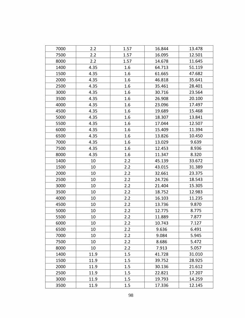
98
7000 2.2 1.57 16.844 13.478
7500 2.2 1.57 16.095 12.501
8000 2.2 1.57 14.678 11.645
1400 4.35 1.6 64.713 51.119
1500 4.35 1.6 61.665 47.682
2000 4.35 1.6 46.818 35.641
2500 4.35 1.6 35.461 28.401
3000 4.35 1.6 30.716 23.564
3500 4.35 1.6 26.908 20.100
4000 4.35 1.6 23.096 17.497
4500 4.35 1.6 19.689 15.468
5000 4.35 1.6 18.307 13.841
5500 4.35 1.6 17.044 12.507
6000 4.35 1.6 15.409 11.394
6500 4.35 1.6 13.826 10.450
7000 4.35 1.6 13.029 9.639
7500 4.35 1.6 12.453 8.936
8000 4.35 1.6 11.347 8.320
1400 10 2.2 45.139 33.672
1500 10 2.2 43.015 31.389
2000 10 2.2 32.661 23.375
2500 10 2.2 24.726 18.543
3000 10 2.2 21.404 15.305
3500 10 2.2 18.752 12.983
4000 10 2.2 16.103 11.235
4500 10 2.2 13.736 9.870
5000 10 2.2 12.775 8.775
5500 10 2.2 11.889 7.877
6000 10 2.2 10.743 7.127
6500 10 2.2 9.636 6.491
7000 10 2.2 9.084 5.945
7500 10 2.2 8.686 5.472
8000 10 2.2 7.913 5.057
1400 11.9 1.5 41.728 31.010
1500 11.9 1.5 39.752 28.925
2000 11.9 1.5 30.136 21.612
2500 11.9 1.5 22.821 17.207
3000 11.9 1.5 19.793 14.259
3500 11.9 1.5 17.336 12.145

99
4000 11.9 1.5 14.870 10.554
4500 11.9 1.5 12.670 9.313
5000 11.9 1.5 11.793 8.317
5500 11.9 1.5 10.981 7.500
6000 11.9 1.5 9.923 6.817
6500 11.9 1.5 8.899 6.238
7000 11.9 1.5 8.391 5.741
7500 11.9 1.5 8.024 5.309
8000 11.9 1.5 7.305 4.930
1400 9.8 1.5 45.522 34.165
1500 9.8 1.5 43.389 31.869
2000 9.8 1.5 32.989 23.820
2500 9.8 1.5 24.976 18.974
3000 9.8 1.5 21.597 15.732
3500 9.8 1.5 18.926 13.409
4000 9.8 1.5 16.264 11.660
4500 9.8 1.5 13.874 10.296
5000 9.8 1.5 12.879 9.202
5500 9.8 1.5 11.987 8.304
6000 9.8 1.5 10.846 7.554
6500 9.8 1.5 9.740 6.918
7000 9.8 1.5 9.168 6.371
7500 9.8 1.5 8.759 5.897
8000 9.8 1.5 7.992 5.481
1400 3.8 1.5 68.323 54.680
1500 3.8 1.5 65.104 51.006
2000 3.8 1.5 49.424 38.135
2500 3.8 1.5 37.436 30.398
3000 3.8 1.5 32.431 25.231
3500 3.8 1.5 28.408 21.533
4000 3.8 1.5 24.382 18.754
4500 3.8 1.5 20.785 16.589
5000 3.8 1.5 19.330 14.853
5500 3.8 1.5 17.995 13.430
6000 3.8 1.5 16.267 12.243
6500 3.8 1.5 14.595 11.236
7000 3.8 1.5 13.756 10.372
7500 3.8 1.5 13.150 9.623
8000 3.8 1.5 11.978 8.966

100
APPENDIX B-3: Training Data for Feed Point along Patch Width & Length
Optimization
Frequency (MHz)
Patch Width (W)
(mm)
Patch Length (L)
(mm)
1400 83.641 71.507
1500 79.714 66.705
2000 60.572 49.810
2500 45.860 39.663
3000 39.677 32.884
3500 34.763 28.065
4000 29.859 24.433
4500 25.466 21.594
5000 23.659 19.310
5500 22.025 17.458
6000 19.922 15.914
6500 17.886 14.603
7000 16.844 13.480
7500 16.095 12.500
8000 14.678 11.644
1400 64.713 51.115
1500 61.665 47.678
2000 46.818 35.631
2500 35.461 28.389
3000 30.716 23.559
3500 26.908 20.099
4000 23.096 17.496
4500 19.689 15.468
5000 18.307 13.843
5500 17.044 12.511
6000 15.409 11.398
6500 13.826 10.454
7000 13.029 9.641
7500 12.453 8.936
8000 11.347 8.318
1400 45.139 33.680
1500 43.015 31.384

101
2000 32.661 23.369
2500 24.726 18.539
3000 21.404 15.303
3500 18.752 12.980
4000 16.103 11.234
4500 13.736 9.870
5000 12.775 8.777
5500 11.889 7.879
6000 10.743 7.128
6500 9.636 6.491
7000 9.084 5.945
7500 8.686 5.471
8000 7.913 5.057
1400 41.728 31.000
1500 39.752 28.925
2000 30.136 21.612
2500 22.821 17.207
3000 19.793 14.258
3500 17.336 12.145
4000 14.870 10.554
4500 12.670 9.313
5000 11.793 8.317
5500 10.981 7.500
6000 9.923 6.817
6500 8.899 6.238
7000 8.391 5.741
7500 8.024 5.309
8000 7.305 4.930
1400 45.522 34.165
1500 43.389 31.869
2000 32.989 23.820
2500 24.976 18.974
3000 21.597 15.732
3500 18.926 13.409
4000 16.264 11.660
4500 13.874 10.296
5000 12.879 9.202
5500 11.987 8.304
6000 10.846 7.554

102
6500 9.740 6.918
7000 9.168 6.371
7500 8.759 5.897
8000 7.992 5.481
1400 68.323 54.680
1500 65.104 51.006
2000 49.424 38.135
2500 37.436 30.398
3000 32.431 25.231
3500 28.408 21.533
4000 24.382 18.754
4500 20.785 16.588
5000 19.330 14.853
5500 17.995 13.430
6000 16.267 12.243
6500 14.595 11.236
7000 13.756 10.373
7500 13.150 9.623
8000 11.978 8.966
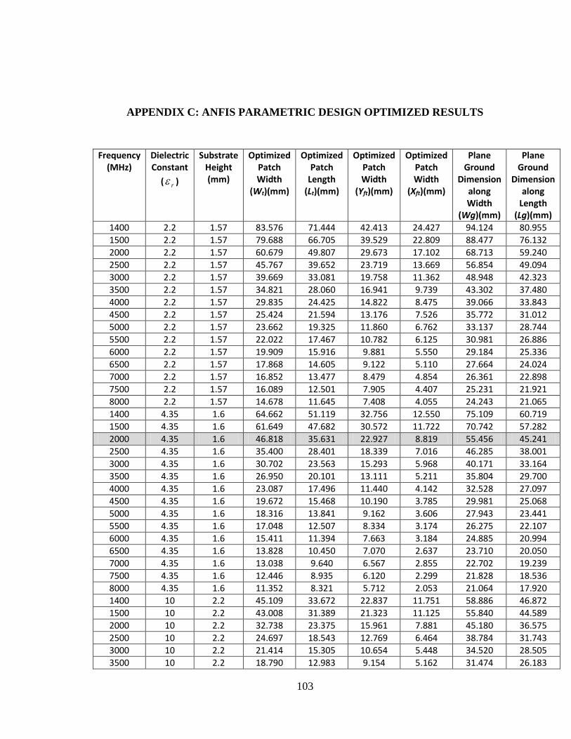
103
APPENDIX C: ANFIS PARAMETRIC DESIGN OPTIMIZED RESULTS
Frequency (MHz)
Dielectric Constant
( r )
Substrate Height (mm)
Optimized Patch Width
(Wt)(mm)
Optimized Patch
Length (Lt)(mm)
Optimized Patch Width
(Yft)(mm)
Optimized Patch Width
(Xft)(mm)
Plane Ground
Dimension along Width
(Wg)(mm)
Plane Ground
Dimension along
Length (Lg)(mm)
1400 2.2 1.57 83.576 71.444 42.413 24.427 94.124 80.955
1500 2.2 1.57 79.688 66.705 39.529 22.809 88.477 76.132
2000 2.2 1.57 60.679 49.807 29.673 17.102 68.713 59.240
2500 2.2 1.57 45.767 39.652 23.719 13.669 56.854 49.094
3000 2.2 1.57 39.669 33.081 19.758 11.362 48.948 42.323
3500 2.2 1.57 34.821 28.060 16.941 9.739 43.302 37.480
4000 2.2 1.57 29.835 24.425 14.822 8.475 39.066 33.843
4500 2.2 1.57 25.424 21.594 13.176 7.526 35.772 31.012
5000 2.2 1.57 23.662 19.325 11.860 6.762 33.137 28.744
5500 2.2 1.57 22.022 17.467 10.782 6.125 30.981 26.886
6000 2.2 1.57 19.909 15.916 9.881 5.550 29.184 25.336
6500 2.2 1.57 17.868 14.605 9.122 5.110 27.664 24.024
7000 2.2 1.57 16.852 13.477 8.479 4.854 26.361 22.898
7500 2.2 1.57 16.089 12.501 7.905 4.407 25.231 21.921
8000 2.2 1.57 14.678 11.645 7.408 4.055 24.243 21.065
1400 4.35 1.6 64.662 51.119 32.756 12.550 75.109 60.719
1500 4.35 1.6 61.649 47.682 30.572 11.722 70.742 57.282
2000 4.35 1.6 46.818 35.631 22.927 8.819 55.456 45.241
2500 4.35 1.6 35.400 28.401 18.339 7.016 46.285 38.001
3000 4.35 1.6 30.702 23.563 15.293 5.968 40.171 33.164
3500 4.35 1.6 26.950 20.101 13.111 5.211 35.804 29.700
4000 4.35 1.6 23.087 17.496 11.440 4.142 32.528 27.097
4500 4.35 1.6 19.672 15.468 10.190 3.785 29.981 25.068
5000 4.35 1.6 18.316 13.841 9.162 3.606 27.943 23.441
5500 4.35 1.6 17.048 12.507 8.334 3.174 26.275 22.107
6000 4.35 1.6 15.411 11.394 7.663 3.184 24.885 20.994
6500 4.35 1.6 13.828 10.450 7.070 2.637 23.710 20.050
7000 4.35 1.6 13.038 9.640 6.567 2.855 22.702 19.239
7500 4.35 1.6 12.446 8.935 6.120 2.299 21.828 18.536
8000 4.35 1.6 11.352 8.321 5.712 2.053 21.064 17.920
1400 10 2.2 45.109 33.672 22.837 11.751 58.886 46.872
1500 10 2.2 43.008 31.389 21.323 11.125 55.840 44.589
2000 10 2.2 32.738 23.375 15.961 7.881 45.180 36.575
2500 10 2.2 24.697 18.543 12.769 6.464 38.784 31.743
3000 10 2.2 21.414 15.305 10.654 5.448 34.520 28.505
3500 10 2.2 18.790 12.983 9.154 5.162 31.474 26.183

104
4000 10 2.2 16.094 11.235 7.947 3.420 29.190 24.435
4500 10 2.2 13.728 9.870 7.017 2.757 27.413 23.070
5000 10 2.2 12.808 8.775 6.383 3.226 25.992 21.975
5500 10 2.2 11.911 7.876 5.818 3.173 24.829 21.077
6000 10 2.2 10.744 7.127 5.311 2.562 23.860 20.327
6500 10 2.2 9.622 6.491 4.876 2.164 23.040 19.691
7000 10 2.2 9.089 5.945 4.548 2.385 22.337 19.145
7500 10 2.2 8.688 5.472 4.291 2.491 21.728 18.672
8000 10 2.2 7.912 5.057 3.945 1.696 21.195 18.257
1400 11.9 1.5 41.656 31.010 21.093 4.651 51.187 40.010
1500 11.9 1.5 39.714 28.925 19.687 4.362 48.375 37.925
2000 11.9 1.5 30.222 21.612 14.777 3.485 38.531 30.612
2500 11.9 1.5 22.797 17.207 11.823 2.785 32.625 26.207
3000 11.9 1.5 19.776 14.259 9.823 1.944 28.687 23.259
3500 11.9 1.5 17.359 12.145 8.439 2.031 25.875 21.145
4000 11.9 1.5 14.869 10.554 7.466 2.511 23.766 19.554
4500 11.9 1.5 12.668 9.313 6.539 1.128 22.125 18.313
5000 11.9 1.5 11.795 8.317 5.915 1.343 20.812 17.317
5500 11.9 1.5 10.978 7.500 5.374 1.307 19.739 16.500
6000 11.9 1.5 9.923 6.818 4.950 1.401 18.844 15.817
6500 11.9 1.5 8.903 6.238 4.545 1.178 18.087 15.238
7000 11.9 1.5 8.396 5.741 4.202 0.916 17.437 14.741
7500 11.9 1.5 8.015 5.309 3.989 1.157 16.875 14.309
8000 11.9 1.5 7.310 4.931 3.692 0.731 16.383 13.930
1400 9.8 1.5 45.513 34.165 23.058 5.745 55.107 43.165
1500 9.8 1.5 43.392 31.869 21.516 5.309 52.033 40.869
2000 9.8 1.5 33.030 23.820 16.160 4.369 41.275 32.820
2500 9.8 1.5 24.917 18.974 12.914 3.218 34.820 27.974
3000 9.8 1.5 21.611 15.732 10.783 3.104 30.517 24.732
3500 9.8 1.5 18.969 13.408 9.213 2.085 27.443 22.409
4000 9.8 1.5 16.249 11.661 8.079 2.249 25.137 20.660
4500 9.8 1.5 13.845 10.295 7.194 2.131 23.344 19.296
5000 9.8 1.5 12.892 9.202 6.481 2.123 21.910 18.202
5500 9.8 1.5 11.998 8.304 5.892 1.865 20.736 17.304
6000 9.8 1.5 10.844 7.554 5.393 1.208 19.758 16.554
6500 9.8 1.5 9.729 6.918 4.947 0.838 18.931 15.918
7000 9.8 1.5 9.175 6.372 4.602 1.074 18.221 15.371
7500 9.8 1.5 8.760 5.897 4.353 1.334 17.607 14.897
8000 9.8 1.5 7.989 5.481 4.027 1.058 17.069 14.481
1400 3.8 1.5 68.270 54.680 34.580 14.314 78.160 63.680
1500 3.8 1.5 65.089 51.006 32.275 13.372 73.550 60.006
2000 3.8 1.5 49.544 38.135 24.206 10.056 57.412 47.135
2500 3.8 1.5 37.375 30.398 19.367 8.084 47.730 39.398
3000 3.8 1.5 32.416 25.231 16.135 6.737 41.275 34.231
3500 3.8 1.5 28.453 21.532 13.821 5.592 36.664 30.533

105
4000 3.8 1.5 24.372 18.755 12.118 5.201 33.206 27.754
4500 3.8 1.5 20.767 16.588 10.755 4.501 30.517 25.589
5000 3.8 1.5 19.336 14.853 9.705 4.298 28.365 23.853
5500 3.8 1.5 17.996 13.431 8.810 3.578 26.604 22.430
6000 3.8 1.5 16.265 12.243 8.039 3.071 25.137 21.243
6500 3.8 1.5 14.593 11.235 7.440 2.872 23.896 20.236
7000 3.8 1.5 13.763 10.373 6.906 3.003 22.832 19.372
7500 3.8 1.5 13.140 9.624 6.447 2.449 21.910 18.623
8000 3.8 1.5 11.983 8.965 6.066 2.563 21.103 17.966

106
APPENDIX D: COMPUTER USAGE PROFILE SUMMARY
APPENDIX D-1: ANFIS MATLAB Time Usage Profile

107
APPENDIX D-2: ANSOFT HFSS Time Usage Profile

108
APPENDIX E: PUBLICATIONS
APPENDIX E-1: Journal Papers
1. K.V. Rop, D.B.O. Konditi, H.A. Ouma, S. Musyoki “Parameter Optimization in
Design of a Rectangular Microstrip Patch Antenna using Adaptive Neuro-Fuzzy
Inference System Technique”, International Journal on Technical and Physical
Problems of Engineering (IJTPE), Issue 12, Vol. 4, No. 3, pp16-23, September
2012
2. K.V. Rop, D.B.O. Konditi. “Performance Analysis of a Rectangular Microstrip
Patch Antenna on Different Dielectric Substrates”, International Institute for
Science Technology and Education (IISTE) - Innovative Systems Design and
Engineering, Vol. 3, No. 8, pp. 7-14, August 2012
APPENDIX E-2: Conference Papers
1. K.V. Rop, D.B.O. Konditi, H.A. Ouma, S. Musyoki “Parameter Optimization in
Design of a Rectangular Microstrip Patch Antenna using Adaptive Neuro-Fuzzy
Inference System Technique”, Annual Interdisciplinary Conference, The
Catholic University of Eastern Africa, Nairobi Kenya, June 2012
2. K.V. Rop, D.B.O. Konditi. “Analysis of a Rectangular Microstrip Patch Antenna
on Different Dielectric Substrates”, KSEEE-JSAEM 2012 International
Engineering Conference, African Institute for Capacity Development (AICAD),
Juja Kenya, pp. 11-16, August, 2012