Parameter identiﬁcation of beam-column structures on … · Parameter identiﬁcation of...

Copyright © 2009 Tech Science Press CMES, vol.39, no.1, pp.1-28, 2009

Parameter identification of beam-column structureson two-parameter elastic foundation

F. Daghia1, W. Hasan1, L. Nobile1 and E. Viola1,2

Abstract: In this paper, a finite element model has been developed for analysingthe flexural vibrations of a uniform Timoshenko beam-column on a two-parameterelastic foundation. The beam was discretized into a number of finite elements hav-ing four degrees of freedom each. The effect of end springs was incorporated inorder to identify the end constraints.The procedure for identifying geometric and mechanical parameters as well as theend restraints of a beam on two-parameter elastic foundation is based on experi-mentally measured natural frequencies from dynamic tests on the structure itself.An iterative statistical identification method, based on the Bayesian approach, wasused to identify a set of geometric, physical and mechanical parameters of the abovementioned structure.Simulated measured natural frequencies of the structure were used throughout theidentification method. The engineer’s confidence in the modelling of the variousparameters was also quantified and incorporated into the revision procedure.

Keywords: Bayesian analysis, parameter estimation, finite elements, two-parameterelastic foundation.

List of main symbols

P Axial forceN Normal forceV Shearing stressM Bending momentp External axial load per unit lengthq External shear load per unit lengthm External moment per unit length

1 DISTART- Department, University of Bologna, Viale Risorgimento 2, 40136 Bologna, Italy2 Corresponding author. Tel.: +39 051 2093510; fax: +39 051 2093495; E-mail:

[email protected]

2 Copyright © 2009 Tech Science Press CMES, vol.39, no.1, pp.1-28, 2009

u Axial displacementv Transverse displacementφ Rotationε Longitudinal strainγ Shearing strainχ Curvatureρ Mass densityA Cross-sectional areaI Moment of inertiaE Young’s modulusG Shear modulusκ Shear coefficientk Winkler foundation moduluskp Pasternak foundation modulusK1, K2, K Linear end spring moduliγ1, γ2, γ Rotational end spring moduliδWe External virtual workδWi Internal virtual workWPe Work of compressive axial forceΦe Strain energyECe Kinetic energyEPT Total dynamic potential energyNv, Nφ Vectors of interpolation functionsq Nodal displacement vectorK Stiffness matrixM Mass matrixr Vector of unknown parametersλ Eigenvalueψ EigenvectorS Sensitivity matrixCεε Covariance matrix of experimental errorCrr Covariance matrix of prior parametersβ Confidence coefficientH Estimator matrixL Length of beamb Width of beamhi Depth of i-th elementEIi Flexural stiffness of i-th element

Parameter identification of beam-column structures 3

1 Introduction

In recent years, inverse problems have been extensively treated in engineering fora wide range of applications. The identification of unknown parameters alwaysrequires a mathematical model of the structure under consideration. The two mainmethods used for inverse analysis are the finite element method (FEM) and theboundary element method (BEM), [Mellings and Aliabadi (1995)]. In this paperthe FEM, which is a well established procedure for structural analysis [Zienkiewicz(1997); Atluri, Gallagher and Zienkiewicz (1983)], will be used for the parameteridentification of beam-column structures on two parameter elastic foundation.

The subject of beam-columns on elastic foundation occupies an important rolein the study of soil-structure interaction problems. Several authors studied thefree vibrations of Euler-Bernoulli beams on Winkler elastic foundation [Doyle andPavlovic (1982); Eisenberger, Yankelevsky and Adin (1985); Laura and Cortinez(1987); Pavlovic and Wylie (1983); De Rosa (1989); Lai, Chen and Hsu (2008)],considering partial foundation and non-uniform elastic foundation, too. Particularfoundation models were also studied [Kerr (1964); Fletcher and Hermann (1971);Jones and Xenophontos (1977)]. For a more accurate representation of the char-acteristics of many practical beams, the elastic foundation was idealized by two-parameter model (Winkler-Pasternak), and the effects of shear deformation (Timo-shenko beam) and rotatory inertia on the dynamic behaviour were evaluated [Wangand Stephens (1977); Wang and Gagnon (1978); Filipich and Rosales (1988)]. Inthe aforementioned studies, the direct problem was solved by determining the nat-ural frequencies and modes of vibration in terms of the system parameters.

In order to ensure high reliability of the structures, their actual behaviour has to beaccurately predicted. The attaining of the actual behavioural predictions of struc-tures depends on the correctness of all the parameters affecting the structural re-sponse. Generally, systems do not have well-defined properties because they man-ifest a statistical nature. Therefore, it is necessary to gain as many details aboutthe response as possible in order to treat engineering problems. The treatment ofstructural systems with statistical properties has been presented in a general formincluding correlation between variables, too.

Theoretical bases of identification techniques based on the sensitivity analysis canbe found in [Eykhoff (1974); Collins and Thomson (1969); Berman and Flan-nelly (1971); Baruch and Bar Itzhach (1978); Baruch (1984); Adelman and Haftka(1986); Wang, Huang and Zhang (1993)]. The theory developed is applicable toany problem leading to an eigenvalue equation. Referring to the aim of this paper,sensitivity theory is a mathematical field that has its predominant use in investigat-ing the change in the statistical properties of vibrating structural system behaviour


due to parameter variations. Sensitivity of the physical property of a dynamic sys-tem to variations of different parameters can be determined by estimating the cor-responding partial derivatives at some fixed combinations of the parameters them-selves. More recently, there has been strong interest in promoting systematic struc-tural optimisation as a useful tool for the practicing structural engineering of largeproblems [Araùjo, Mota Soares and Moreira de Freitas (1996); Frederiksen (1998);Hongxing, Sol and de Wilde (2000); Araùjo, Mota Soares, Moreira de Freitas, Ped-ersen and Herskovits (2000)]. Considerable effort has been devoted to the generalproblem of structural parameters identification. In the past three decades, statis-tical identification method, which considers the parameters as stochastic variablesand provides the assessment from dynamic response, has been extensively used[Hasselman and Hart (1972); Hart (1973); Collins, Hart, Hasselman and Kennedy(1974); Hart and Torkamani (1974); Hart and Yao (1977); Torkamani and Ahmadi(1988) - a, b, c].

The method of Bayesian estimation has been used for system identification in thefield of automatic control, too. It should be noted that since the early 1970s, inves-tigations involving statistical properties of vibrating structural systems have beenperformed. A few earlier papers [Hasselman and Hart (1972); Hart (1973); Collins,Hart, Hasselman and Kennedy (1974); Hart and Torkamani (1974)] illustrate veryclearly the principle and the technique of the Bayesian sensitivity analysis throughits application to simple systems. More recently, Bayesian identification tech-niques have been applied to more complex estimation problems [Lai and Ip (2006);Daghia, de Miranda, Ubertini and Viola (2007)]. In general, both systematic andrandom errors are present in the identified parameters. A measure of the precisionof the estimated values can be provided by the variance matrix of the estimatedparameters.

In dealing with an identification procedure, a particular mention has to concern theline of research involving the dynamic behaviour of systems and the damage de-tection in structures by modal vibration characterization. To this end, it is worthnoting that identification procedures to improve a finite element model using ex-perimental modal data are presented in [Antonacci, Capecchi, Silvano and Vestroni(1992); Wu and Li (2004)]. Experimental structural vibration data can be used toidentify unknown loads applied to a structure [Huang and Shih (2007)] as well asstructural damping, stiffness coefficients and restoring forces [Liu (2008) – a, b].The problem of modelling for parameters identification in distributed structures isworked out in [Baruh and Boka (1992); Baruh and Meirovitch (1985)]. Identifica-tion procedures to study steel structures using experimental modal data are reportedin [Morassi and Rovere (1997); Kosmatka and Ricles (1999); Bicanic and Chen(1997); Capecchi and Vestroni (1999); Rytter, Krawczuk and Kirkegaard (2000)].


These techniques can be employed to evaluate the real structural behaviour. More-over, both the location and the extent of structural damage can be correctly deter-mined using only a limited number of natural frequencies.

Although researchers have focused on the identification of structural parameters,to the authors’ knowledge no-one has dealt with the identification of geometri-cal, physical and mechanical parameters of Timoshenko beam structures on twoparameter elastic foundation. So, the aim of the present work is to formulate anappropriate FE model for the identification of physical and mechanical parametersof beam-column structures resting on two-parameter elastic foundation (Winklerand Pasternak). The identification procedure incorporates a more accurate modelwith respect the ones employed in the above mentioned papers. The effects ofaxial force and rotatory inertia are also included. It should be noted that an Euler-Bernoulli beam element resting on one-parameter foundation (Winkler model) andconsisting of two nodes, each having two degrees of freedom of transverse dis-placement and bending rotation, was studied in [Viola and Hasan (1996); Hasan,Ricci and Viola (1998); Viola, Ricci and Nobile (1999)] to identify restraint condi-tions. In this paper, the equations of motion are obtained by Hamilton’s principle.In the iterative algorithm an estimator matrix depending on the particular identifi-cation method adopted is introduced. It depends on the sensitivity matrix, the diag-onal covariance matrix of errors on the measured data and the diagonal covariancematrix of initial parameters. The introduction of a coefficient for accelerating theconvergence improves the identification technique and can be defined as improvedstatistical method [Torkamani and Ahmadi (1988) - a, b, c].

A numerical example is presented, where the sensitivity matrix are calculated usingthe first three natural frequencies of the structure.

As far as the numerical identification procedure is concerned, some further papersshould be mentioned. They deal with problems regarding the parameter estimationfrom measured displacements of crack edges in isotropic or orthotropic materi-als [Hasan, Piva and Viola (1998); Federici, Piva and Viola (1999)] or structures[Zhang, He, Xiao and Ojalvo (1993); Salane and Baldwin (1990)], which can beinvestigated by means of the statistical numerical approach under consideration.

This paper is arranged into six sections and three appendices. Section 1 coversthe state of the art, that is the introduction to the problem. Section 2 reports theTimoshenko beam equations, namely the equilibrium, congruence, constitutive andfundamental equations for the static case. Section 3 deals with the finite elementformulation where various matrices of the system under consideration are assessed.The identification method is illustrated in Section 4. In Section 5, an illustrativeexample is worked out and numerical results are graphically shown. Finally, insection 6 some conclusions are drawn.


The Appendices of the paper report, in extended notation, the relationships involvedin the matrices considered in the eigenvalue problem.

2 Timoshenko beam equations for static case

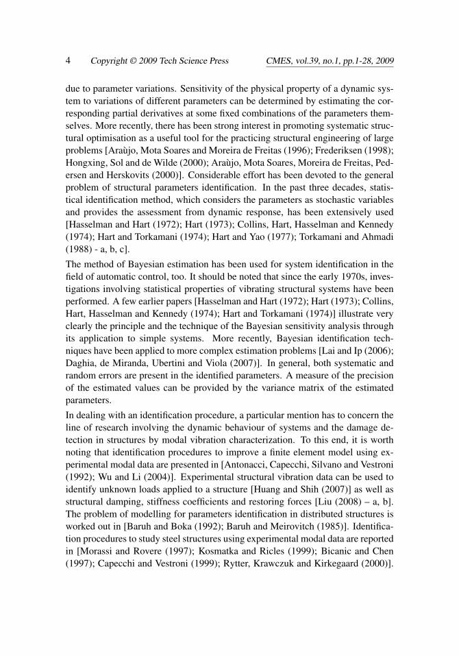
Consider a plane prismatic beam of length L. The structure is made of linear-elastic,homogeneous and isotropic material. Denote E and G the Young’s modulus ofelasticity and the shear modulus, respectively, and by ρ the mass density. Let Oxyzbe a cartesian coordinate system in which the origin O is located at the centroidof the left end cross-section of the beam, the x-axis coincides with the geometricaxis, the y and z axes coincide with the principal axes of the cross-section. Thecross sectional area and the moment of inertia with respect to the neutral axis arefunctions of x and can be denoted by A(x) and I(x), respectively. Consequently, theflexural rigidity EI(x) and mass per unit length ρA(x) are variable along the x-axis.

The plane and straight beam in Fig. 1, restrained in an arbitrary way at its ends, issupposed to be in equilibrium under a general load system. The y and z componentsof external forces per unit length are denoted by q = q(x) and p = p(x), respectively,and the external moments per unit length by m = m(x). 4

components of strain through the strain-displacement relations. The deformation of the beam is completely defined by the strain components which are the longitudinal strain ε(x), the shearing strain γ(x) and the curvature χ(x). The strain-displacement relations can be obtained by the application of the principle of virtual forces. The external virtual work δWe is

( )0

dl

eW pu qv m xδ φ= + +∫ , (2)

the internal virtual work is

( )0

dl

iW N V M xδ ε γ χ= + +∫ (3)

Combining eqs. (1) and (2) and integrating by parts, the condition for compatibility δWe=δWi gives

0

d d d d 0d d d

l u vN V M xx x x

φε φ γ χ⎡ ⎤⎛ ⎞ ⎛ ⎞ ⎛ ⎞− + + − + − =⎜ ⎟ ⎜ ⎟ ⎜ ⎟⎢ ⎥⎝ ⎠ ⎝ ⎠ ⎝ ⎠⎣ ⎦∫ (4)

from which it follows that d d d, ,d d d

u vx x x

φε γ φ χ= = + = (5)

for any kinematic boundary conditions. When the beam is made of linear-elastic, homogeneous and isotropic material, the constitutive equations are: N= EAε, V=GΛγ, M=EIχ (6) where Λ=A/κ, with κ being the shear coefficient depending on the geometry of the cross-section. Combining eqs. (1), (5) and (6), the system of three ordinary differential equations of second order can be obtained

d d ( ) 0d d

uEA p xx x⎛ ⎞ + =⎜ ⎟⎝ ⎠

(7)

d d ( ) 0d d

vG q xx x

φ⎡ ⎤⎛ ⎞Λ + + =⎜ ⎟⎢ ⎥⎝ ⎠⎣ ⎦ (8)

d d d( )d d d

vEI m x Gx x x

φ φ⎛ ⎞ ⎛ ⎞+ = Λ +⎜ ⎟ ⎜ ⎟⎝ ⎠ ⎝ ⎠

(9)

It should be noted that eqs. (8), (9) are coupled through the variables v and φ.

3 Finite element formulation

The beam column is partitioned into a finite number of elements. For the typical element shown in Fig. 1, the strain energy including the effects of the two-parameter foundation, shear deformation and end springs is

Figure 1: Typical column finite element

( )

( ) ( ) ( )

2 2

0 0

222

1 00 0

2 2 21 2 20

1 1d d2 2

1 1 1d d ,2 2 21 1 1, , ,2 2 2

l l

e

l l

P x

x x l x l

vEI x G xx x

vkv x k x K v x tx

x t K v x t x t

φ φ

γ φ γ φ

=

= = =

∂ ∂⎛ ⎞ ⎛ ⎞Φ = + Λ + +⎜ ⎟ ⎜ ⎟∂ ∂⎝ ⎠ ⎝ ⎠

∂⎛ ⎞+ + +⎜ ⎟∂⎝ ⎠

+ + +

+

∫ ∫

∫ ∫ (10)

where x is the local coordinate along the geometrical axis, k is the Winkler foundation modulus, kP is the shear foundation modulus, Ki (i=1,2) is the linear end spring modulus and γi (i=1,2) is the rotational end spring modulus. Note that the effect of end springs is incorporated in order to identify end constraints. The work done by the compressive axial force is

2

0

d12Pe

lvP xx

W ∂⎛ ⎞⎜ ⎟∂⎝ ⎠

= − ∫ (11)

The Kinetic energy of the beam element including the rotatory inertia effect is given by

2 22 2

0 0 0 0

1 1 1 1d d d d2 2 2 2e

l l l lvEC A x I x Av x I xt t

φρ ρ ρ ρ φ∂ ∂⎛ ⎞ ⎛ ⎞= + = +⎜ ⎟ ⎜ ⎟∂ ∂⎝ ⎠ ⎝ ⎠∫ ∫ ∫ ∫ && (12)

where ρ is the mass density of the beam material and t is the time. The representation of displacement v and rotation φ is performed by means of algebraic shape functions that exactly satisfy the homogeneous form of the static equations (8) and (9). Thus, displacement v and rotation φ can be expressed as

( ) Tv ev x = N q (13)

and ( ) T

ex φφ = N q (14)

where Nv and Nφ are vectors of interpolation functions of displacement v(x) and rotation φ(x), respectively, and qe is the nodal displacement vector. The shape functions for displacement are given by the following:

kP

y

x

K1

γ1

K2

γ2

P PO

k

m q

p

Figure 1: Typical column finite element

At some point on the beam’s axis, a normal force N = N(x), a shearing stressV = V (x) and bending moment M = M(x) are considered to act on the left side ofan element dx. On the opposite side where the location is x+dx from the origin thestress resultants acquire incremental changes of dN, dV and dM in the interval dx.The equilibrium conditions on stress resultants are

dNdx

+ p = 0,dVdx

+q = 0,dMdx

+m = V (1)


Axial displacement u = u(x), transverse displacement v = v(x) and rotation of thecross-section φ = φ(x) are independent variables that allow us to determine thecomponents of strain through the strain-displacement relations. The deformation ofthe beam is completely defined by the strain components which are the longitudinalstrain ε(x), the shearing strain γ(x) and the curvature χ(x).The strain-displacement relations can be obtained by the application of the principleof virtual forces. The external virtual work δWe is

δWe =l∫

0

(pu+qv+mφ)dx, (2)

the internal virtual work is

δWi =l∫

0

(Nε +V γ +Mχ)dx (3)

Combining eqs. (1) and (2) and integrating by parts, the condition for compatibilityδWe = δWi gives

l∫0

[N(

dudx− ε

)+ V

(dvdx

+φ − γ

)+ M

(dφ

dx−χ

)]dx = 0 (4)

from which it follows that

ε =dudx

, γ =dvdx

+φ , χ =dφ

dx(5)

for any kinematic boundary conditions.

When the beam is made of linear-elastic, homogeneous and isotropic material, theconstitutive equations are:

N = EAε, V = GΛγ, M = EIχ (6)

where Λ = A/κ , with κ being the shear coefficient depending on the geometry ofthe cross-section.

Combining eqs. (1), (5) and (6), the system of three ordinary differential equationsof second order can be obtained

ddx

(EA

dudx

)+ p(x) = 0 (7)


ddx

[GΛ

(dvdx

+φ

)]+ q(x) = 0 (8)

ddx

(EI

dφ

dx

)+ m(x) = GΛ

(dvdx

+φ

)(9)

It should be noted that eqs. (8), (9) are coupled through the variables v and φ .

3 Finite element formulation

The beam column is partitioned into a finite number of elements. For the typical el-ement shown in Fig. 1, the strain energy including the effects of the two-parameterfoundation, shear deformation and end springs is

Φe =12

l∫0

EI(

∂φ

∂x

)2

dx+12

l∫0

GΛ

(∂v∂x

+φ

)2

dx

+12

l∫0

kv2dx+12

l∫0

kP

(∂v∂x

)2

dx+12

K1v(x, t)2x=0

+12

γ1 φ (x, t)2x=0 +

12

K2v(x, t)2x=l +

12

γ2 φ (x, t)2x=l (10)

where x is the local coordinate along the geometrical axis, k is the Winkler founda-tion modulus, kP is the shear foundation modulus, Ki (i=1,2) is the linear end springmodulus and γi (i=1,2) is the rotational end spring modulus. Note that the effect ofend springs is incorporated in order to identify end constraints.

The work done by the compressive axial force is

WPe =−12

l∫0

P(

∂v∂x

)2

dx (11)

The Kinetic energy of the beam element including the rotatory inertia effect is givenby

ECe =12

l∫0

ρA(

∂v∂ t

)2

dx+12

l∫0

ρI(

∂φ

∂ t

)2

dx =12

l∫0

ρAv2dx+12

l∫0

ρIφ2dx (12)

where ρ is the mass density of the beam material and t is the time.

The representation of displacement v and rotation φ is performed by means of al-gebraic shape functions that exactly satisfy the homogeneous form of the staticequations (8) and (9).


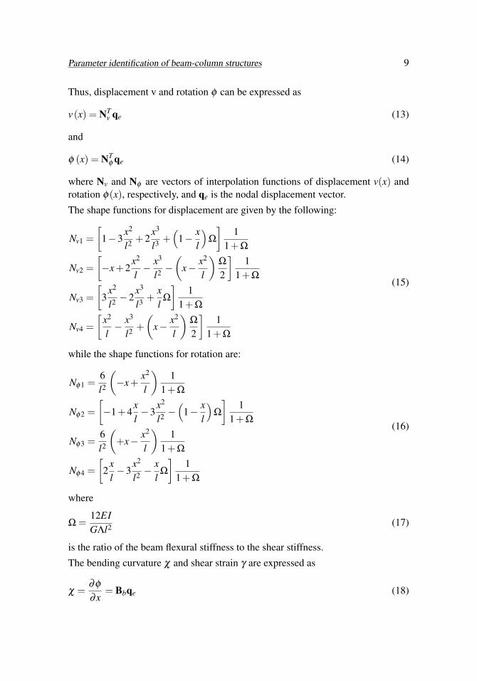
Thus, displacement v and rotation φ can be expressed as

v(x) = NTv qe (13)

and

φ (x) = NTφ qe (14)

where Nv and Nφ are vectors of interpolation functions of displacement v(x) androtation φ(x), respectively, and qe is the nodal displacement vector.

The shape functions for displacement are given by the following:

Nv1 =[

1−3x2

l2 +2x3

l3 +(

1− xl

)Ω

]1

1+Ω

Nv2 =[−x+2

x2

l− x3

l2 −(

x− x2

l

)Ω

2

]1

1+Ω

Nv3 =[

3x2

l2 −2x3

l3 +xlΩ

]1

1+Ω

Nv4 =[

x2

l− x3

l2 +(

x− x2

l

)Ω

2

]1

1+Ω

(15)

while the shape functions for rotation are:

Nφ1 =6l2

(−x+

x2

l

)1

1+Ω

Nφ2 =[−1+4

xl−3

x2

l2 −(

1− xl

)Ω

]1

1+Ω

Nφ3 =6l2

(+x− x2

l

)1

1+Ω

Nφ4 =[

2xl−3

x2

l2 −xlΩ

]1

1+Ω

(16)

where

Ω =12EIGΛl2 (17)

is the ratio of the beam flexural stiffness to the shear stiffness.

The bending curvature χ and shear strain γ are expressed as

χ =∂φ

∂x= Bbqe (18)


γ =∂v∂x

+φ = Bsqe (19)

where

Bb =∂

∂xNφ (20)

Bs =∂

∂xNv +Nφ = Bv +Nφ (21)

Substituting eqs. (18)-(21) into eqs. (10)-(12) gives

Φe =12

qTe kebqe +

12

qTe kesqe +

12

qTe keW qe +

12

qTe kePqe +

12

qTe ke1qe +

12

qTe ke2qe

(22)

ECe =12

qTe mevqe +

12

qTe meφ qe (23)

WPe =−12

qTe kegqe (24)

where

keb =l∫

0

BTb EIBbdx (25)

is the flexural stiffness matrix,

kes =l∫

0

BTs GΛBsdx (26)

is the shear stiffness matrix.

keW =l∫

0

NTv kNvdx (27)

is the stiffness matrix due to Winkler foundation,

keP =l∫

0

BTv kpBvdx (28)

is the stiffness matrix due to shear foundation,

ke1 = K1(NT

v Nv)

x=0 + γ1(NT

φ Nφ

)x=0

(29)


is the stiffness matrix due to left end springs,

ke2 = K2(NT

v Nv)

x=l + γ2(NT

φ Nφ

)x=l

(30)

is the stiffness matrix due to right end springs,

keg =l∫

0

BTv PBvdx (31)

is the geometric stiffness matrix,

mev =l∫

0

ρANvNTv dx (32)

is the consistent mass matrix for translational inertia,

meφ =l∫

0

ρINφ NTφ dx (33)

is the consistent mass matrix for rotatory inertia, and the superposed dot denotesdifferentiation with respect to time t.

The stiffness matrix ke and the consistent mass matrix me for the beam element canbe obtained as

ke = keb +kes +keW +keP +ke1 +ke2−keg (34)

me = mev +meφ (35)

Matrices (34)-(35) are listed in extensive notation in Appendix A.

Inserting the total dynamic potential energy

EPT = ∑e

(Φe +ECe−WPe) (36)

into Hamilton’s principle leads to the governing matrix equation for free vibrationsof the Timoshenko beam-column on the two-parameter elastic foundation as

Kq+Mq = 0 (37)

where q is the global displacement vector and

K =n

∑i=1

(Keb +Kes +KeW +KeP +Ke1 +Ke2−Keg) (38)


is the global stiffness matrix,

M =n

∑i=1

(Mev +Meφ

)(39)

is the global consistent mass matrix.

The global stiffness matrix can be expressed as

K = diag(ααα, βββ , . . . , βββ , ξξξ ) (40)

where matrices ααα , βββ , ξξξ are expressed as

ααα =

a′ b c db e′ f gc f 2a 0d g 0 2e

(41)

βββ =

2a 0 c d0 2e f gc f 2a 0d g 0 2e

(42)

ξξξ =

2a 0 c d0 2e f gc f a′′ hd g h e′′

(43)

The explicit expressions for the respective element matrices are listed in appendixB.

The global consistent mass matrix can be expressed as

M = diag(αααm, βββ m, . . . , βββ m, ξξξ m) (44)

where

αααm =

A B C DB E F GC F 2A 0D G 0 2E

(45)

βββ m =

2A 0 C D0 2E F GC F 2A 0D G 0 2E

(46)


ξξξ m =

2A 0 C D0 2E F GC F A HD G H E

(47)

The explicit expressions for the respective element matrices are listed in appendixC.

4 The identification method

Denote by

r = (r1 r2 . . . rm)T (48)

the vector of unknown parameters ri (i=1, 2, ... m) to be identified, e.g. geometricor structural parameters. Mass and stiffness matrices in eq. (49) are functions ofthese parameters of the system and therefore the eigenvalues and eigenvectors areimplicit functions of these same parameters. Eq. (37) can be written as

[K−λi(r)M]ψψψ i(r) = 0 (49)

where λi(r), ψψψ i(r) are the eigenvalues and the eigenvectors, respectively.

The functional relationship between the modal characteristics and the parameterscan be expressed in terms of a Taylor’s series expansion

λλλ (r)ψψψ(r)

=

λλλ (ra)ψψψ(ra)

+S(r− ra) (50)

where

ra = (r1a r2a . . . rma)T (51)

is the vector of prior estimates of parameters, λλλ (ra) and ψψψ(ra) are are the vectorsof eigenvalues and eigenvectors when r = ra ,

S =∣∣∣∣ ∂λλλ/∂r∂ψψψ/∂r

∣∣∣∣ (52)

is the sensitivity matrix. The partial derivatives of λλλ (ra) e ψψψ(ra) with respect to rare

∂λi

∂ r j= ψψψ

Ti

(∂K∂ r j−λi

∂M∂ r j

)ψψψ i (53)


∂ψψψ i

∂ r j=− [K−λiM]−1

ψψψTi

(∂K∂ r j− ∂λi

∂ r jM−λi

∂M∂ r j

)ψψψ i (54)

Substituting λi = ω2i into eqs. (53) and (54) gives

∂ωi

∂ r j=

12ωi

ψψψTi

(∂K∂ r j−ω

2i

∂M∂ r j

)ψψψ i (55)

∂ψψψ i

∂ r j=−

[K−ω

2i M]−1

ψψψTi

(∂K∂ r j−2ωi

∂ωi

∂ r jM−ω

2i

∂M∂ r j

)ψψψ i (56)

The iterative algorithm for the identification method can be written as

r = r+H

∆λλλ

∆ψψψ

=(r1 r2 .......... rm

)T (57)

where r is the vector of estimated parameters at the i-th iteration, r the same vectorat the (i+1)-th iteration,

H = β−1CrrST (β−1SCrrST +Cεε)−1 (58)

is an estimator matrix, with Cεε = diag(b1 . . .bn) the diagonal covariance matrix oferrors on the measured data, Crr = diag(a1 . . .an) the diagonal covariance matrix ofthe priori parameters and β [Berman and Flannelly (1971); Baruch and Bar (1978)]a confidence coefficient, and

∆λλλ

∆ψψψ

=

λλλ s

ψψψs

−

λλλ (r)ψψψ(r)

(59)

where λλλ s and ψψψs are vectors of experimentally measured values, λλλ (r) and ψψψ(r) arevectors of eigenvalues and eigenvectors, respectively, obtained from solution to eq.(49) with r = ra.

Convergence is evaluated at the end of each iteration prescribing confidence bounds,as a rule 95%, to λλλ (r) and ψψψ(r).

If the number of measured eigenvalues and independent elements of eigenvectorsis equal to the number of parameters

H = S−1 (60)

Usually, the number of parameters exceeds the number of measured eigenvaluesand eigenvectors (under-determined system). The solution of the problem dependson the prior estimates, the covariance matrices Cεε and Crr, and the coefficient β .The structural analyst establishes the prior parameter values, the covariance matrix


of the priori parameters and the confidence coefficient; the structural experimental-ist establishes the covariance matrix of errors on the measured data.

It should be noted that, as appears from equation (57), during the iteration processthe estimator matrix (58) relates the revised parameters to the prior ones. Moreover,comparison of the vectors for the initial estimates and for the revised parameterswill indicate which of the properties are found more accurately. According to theBayesian point of view, different tests must be repeated on series of tests in orderto obtain statistically relevant results.

7

where r is the vector of estimated parameters at the i-th iteration, r) the same vector at the (i+1)-th iteration,

H = 1 T 1 T 1( + )rr rr εεβ β− − −C S SC S C (58)

is an estimator matrix, with Cεε=diag(b1…bn) the diagonal covariance matrix of errors on the measured data, Crr=diag(a1…an) the diagonal covariance matrix of the priori parameters and β [Berman and Flannelly (1971); Baruch and Bar (1978)] a confidence coefficient, and

( )( )

s

s

⎧ ⎫⎧ ⎫⎧ ⎫Δ ⎪ ⎪= −⎨ ⎬ ⎨ ⎬ ⎨ ⎬Δ ⎪ ⎪⎩ ⎭ ⎩ ⎭ ⎩ ⎭ (59)

where λs and ψs are vectors of experimentally measured values, λ(r) and ψ(r) are vectors of eigenvalues and eigenvectors, respectively, obtained from solution to eq. (49) with r = ra. Convergence is evaluated at the end of each iteration prescribing confidence bounds, as a rule 95%, to λ(r) and ψ(r). If the number of measured eigenvalues and independent elements of eigenvectors is equal to the number of parameters H = S-1 (60) Usually, the number of parameters exceeds the number of measured eigenvalues and eigenvectors (under-determined system). The solution of the problem depends on the prior estimates, the covariance matrices Cεε and Crr, and the coefficient β. The structural analyst establishes the prior parameter values, the covariance matrix of the priori parameters and the confidence coefficient; the structural experimentalist establishes the covariance matrix of errors on the measured data. It should be noted that, as appears from equation (57), during the iteration process the estimator matrix (58) relates the revised parameters to the prior ones. Moreover, comparison of the vectors for the initial estimates and for the revised parameters will indicate which of the properties are found more accurately. According to the Bayesian point of view, different tests must be repeated on series of tests in order to obtain statistically relevant results.

Figure 2: Timoshenko beam-column

Table 1: Geometric and mechanical characteristics

lenght L 7.5 m

width b 0.2 m

Depth of element h1 0.30 m



Young’s modulus E 31000000 KN·m-2

flexural stiffness of element EI1 13950 KN·m2



Mass density ρ 25 KN·m-3

Winkler foundation modulus k 21.7 KN·m-2

Pasternak foundation modulus kp 25 KN·m-2

Linear end spring modulus K1=K2=K 300 KN·m-1

Rotational end spring modulus γ1=γ2=γ 250 KN·m

Shear modulus G 3/8E

Shear coefficient κ 1.5

Axial force P 50 KN

5 Illustrative example

Consider a Timoshenko beam-column with end springs and discontinuity in thickness, supported on an elastic foundation as depicted in Fig. 2. The elastic foundation is idealized as constant two-parameter model characterized by two moduli k and kP. The geometric and mechanical properties of the beam-column are illustrated in Tab. 1. The previously illustrated iterative method of identification is now applied to identify the nine parameters collected in the vector

( )( )

1 1 2 3

1 2 3 4 5 6 7 8 9

pK k k EI EI EI G P

r r r r r r r r r

γ= =r (61)

In the present identification procedure, only the first three natural frequencies and modal shapes are required to obtain an estimate. To simulate the experimental data, the measured natural frequencies are obtained from the eigenvalues obtained by solving the characteristic equation with the “actual” parameters as in Tab. 1.

( )( )

1 2 3 4 5 6 7 8 9

300 250 21.7 25 13950 33067 64583 11625000 50

r r r r r r r r r= =

=

r

(62) The analysis is performed by using ten finite elements for each beam element of constant depth.

L L/3 L/3

k

EI2,ρA2 EI1,ρA1

EI3,ρA3

L/3

kp

y

x

γ1 γ2

Κ1 K2

P P

L

Figure 2: Timoshenko beam-column

Table 1: Geometric and mechanical characteristicslenght L 7.5 mwidth b 0.2 m

Depth of element 1 h1 0.30 mDepth of element 2 h2 0.40 mDepth of element 3 h3 0.50 mYoung’s modulus E 31000000 KN·m−2

flexural stiffness of element 1 EI1 13950 KN·m2



Mass density ρ 25 KN·m−3

Winkler foundation modulus k 21.7 KN·m−2

Pasternak foundation modulus kp 25 KN·m−2

Linear end spring modulus K1=K2=K 300 KN·m−1

Rotational end spring modulus γ1 = γ2 = γ 250 KN·mShear modulus G 3/8E

Shear coefficient κ 1.5Axial force P 50 KN


5 Illustrative example

Consider a Timoshenko beam-column with end springs and discontinuity in thick-ness, supported on an elastic foundation as depicted in Fig. 2. The elastic founda-tion is idealized as constant two-parameter model characterized by two moduli kand kP.

The geometric and mechanical properties of the beam-column are illustrated in Tab.1.

The previously illustrated iterative method of identification is now applied to iden-tify the nine parameters collected in the vector

r =(K γ1 k kp EI1 EI2 EI3 G P

)=(r1 r2 r3 r4 r5 r6 r7 r8 r9

)(61)

In the present identification procedure, only the first three natural frequencies andmodal shapes are required to obtain an estimate.

To simulate the experimental data, the measured natural frequencies are obtainedfrom the eigenvalues obtained by solving the characteristic equation with the “ac-tual” parameters as in Tab. 1.

r =(r1 r2 r3 r4 r5 r6 r7 r8 r9

)=(300 250 21.7 25 13950 33067 64583 11625000 50

)(62)

The analysis is performed by using ten finite elements for each beam element ofconstant depth.

The coefficients of variation in the diagonal covariance matrix of errors in measureddata are chosen as: a1=a2=a3=0.10.

The priori coefficients of variation are chosen as: b1=0.0037, b2=0.0155, b3=0.0093,b4=0.0245, b5=0.0065, b6=0.0042, b7=0.0145,b8=0.04, b9=0.019.

Note that the choice of these coefficients is based on the experience of the analystand convergence is based on the prescribed confidence bound equal to 99% of theexperimentally measured frequencies.

Assuming the initial parameters 15% greater than the exact values and β=0.001, theiterative procedure allows the determination of the final estimates as listed in Tab.2. Note that all the parameters are well estimated, with errors varying from 0.05%to 2.84%. The convergence for this case has been obtained after 11 iterations.

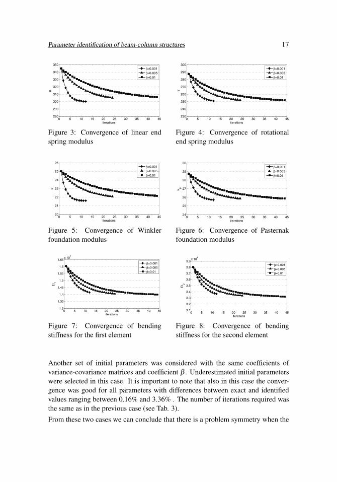
Figg. 3-11 show the influence of the coefficient β on the convergence velocity ofthe identified parameters.


0 5 10 15 20 25 30 35 40 45280

290

300

310

320

330

340

350

iterations

K

β=0.001β=0.005β=0.01

Figure 3: Convergence of linear endspring modulus

0 5 10 15 20 25 30 35 40 45230

240

250

260

270

280

290

300

iterations

γ

β=0.001β=0.005β=0.01

Figure 4: Convergence of rotationalend spring modulus

0 5 10 15 20 25 30 35 40 4520

21

22

23

24

25

26

iterations

k

β=0.001β=0.005β=0.01

Figure 5: Convergence of Winklerfoundation modulus

0 5 10 15 20 25 30 35 40 4524

25

26

27

28

29

30

iterations

k p

β=0.001β=0.005β=0.01

Figure 6: Convergence of Pasternakfoundation modulus

0 5 10 15 20 25 30 35 40 451.3

1.35

1.4

1.45

1.5

1.55

1.6

1.65x 10

4

iterations

EI 1

β=0.001β=0.005β=0.01

Figure 7: Convergence of bendingstiffness for the first element

0 5 10 15 20 25 30 35 40 453.1

3.2

3.3

3.4

3.5

3.6

3.7

3.8

3.9x 10

4

iterations

EI 2

β=0.001β=0.005β=0.01

Figure 8: Convergence of bendingstiffness for the second element

Another set of initial parameters was considered with the same coefficients ofvariance-covariance matrices and coefficient β . Underestimated initial parameterswere selected in this case. It is important to note that also in this case the conver-gence was good for all parameters with differences between exact and identifiedvalues ranging between 0.16% and 3.36% . The number of iterations required wasthe same as in the previous case (see Tab. 3).

From these two cases we can conclude that there is a problem symmetry when the


0 5 10 15 20 25 30 35 40 455.8

6

6.2

6.4

6.6

6.8

7

7.2

7.4

7.6

7.8x 10

4

iterations

EI 3

β=0.001β=0.005β=0.01

Figure 9: Convergence of bending stiffness for the third element

0 5 10 15 20 25 30 35 40 451

1.05

1.1

1.15

1.2

1.25

1.3

1.35

1.4x 10

7

iterations

G

β=0.001β=0.005β=0.01

Figure 10: Convergence of shear mod-ulus

0 5 10 15 20 25 30 35 40 4546

48

50

52

54

56

58

60

iterations

P

β=0.001β=0.005β=0.01

Figure 11: Convergence of axial force

initial values of the estimated parameters are all underestimated or overestimated.

Table 2: Final estimates and error (first set of initial parameters)

parameter K γ k kp EI1

Actual values 300 250 21.7 25 13950Final estimates 300.139 251.025 21.583 25.710 14146.499

Final error 0.05% 0.41% 0.54% 2.84% 1.41%parameter EI2 EI3 G P

Actual values 33067 64583 11625000 -50Final estimates 33648.966 63848.796 11692426.403 -50.316

Final error 1.76% 1.14% 0.58% 0.63%

6 Conclusions and remarks

A method for the statistical identification of a beam-column resting on two-parameterfoundation has been proposed. It uses experimental response measurements of nat-ural frequencies to improve some parameters of a finite element model. The finite


Table 3: Final estimates and error (second set of initial parameters)

parameter K γ k kp EI1

Actual values 300 250 21.7 25 13950Final estimates 299.503 248.948 21.853 24.159 13728.14

Final error 0.16% 0.42% 0.70% 3.36% 1.59%parameter EI2 EI3 G P

Actual values 33067 64583 11625000 -50Final estimates 32443.841 65187.764 11540230.02 -49.66

Final error 1.88% 0.94% 0.73% 0.68%

element model includes end spring effects in order to detect end constraints. Inthe present study, the proposed method basically relies on three items, namely anaccurate mathematical model of the structure, a set of reliable modal model dataand a parameter estimation method based on the Bayesian sensitivity analysis.

The introduction of a confidence coefficient accelerating the convergence charac-terizes the identification technique which can be defined as an improved statisticalmethod.

A numerical example is presented, where the sensitivity matrix is calculated usingthe first three natural frequencies. This worked-out example is based on pseudo-experimentally determined data.

In the statistical Bayesian estimation, priority is given to assessment of uncertain-ties. The method takes into account both the confidence associated with mathemat-ical modelling and parameter estimates. The parameters that have to be estimatedare considered as stochastic values of fixed probability distribution. Incorporat-ing the uncertainties into the initial estimates, the scheme will lead to improvedestimate values for the parameters. As in each inverse problems, the parametersin the mathematical model have to be adjusted repeatedly until its analytical re-sponse match satisfactorily with those associated with the physical structure. Thisis accomplished through two weighting matrices containing the confidences on themeasured natural frequencies and on the initial estimates.

It is worthy of remark to point out that the present study has the innovative aspectof contemplating identification of all the parameters affecting the dynamic free vi-bration of a structure, that is to say the parameters describing its geometry, density,boundary conditions and elastic constants.

It is well known that investigations and monitoring of structures are essential toolsto improve the knowledge of their structural behaviour. As far as the practica-bility of a procedure for parameter identification is concerned, some noteworthy


points are related to the importance of structures under investigation. Firstly, mea-surements gathered by means of an automatic monitoring system installed in thestructure can make the refinement of the mathematical model possible. Secondly,assumptions about the law of deformation of materials and hypotheses involvingvarious boundary conditions have to be made. Thirdly, a mathematical referencemodel for the numerical simulation of the structures is always required. Usually,such a model is based on the finite element method.

A number of researchers have presented methods to improve the analytical modelof structural systems and several non-destructive evaluations techniques have beenproposed especially for the determination of material properties of damaged andnon-damaged structures.

On the upshot, the identification techniques as useful tools in the structural analysisprocess are gaining more and more popularity. However, it should be mentionedthat some aspects involving the inverse problems of structural systems are not com-pletely resolved, such as the uniqueness of the results [Udwadia, Sharma and Shah(1978)], the incompleteness of the measured data [Berman and Flannelly (1971)],the ill-conditioned equations arising in structural system identification [Hasan andViola (1997)], among others. In the latter paper, the singular value decomposi-tion method is used to investigate the ill-conditioning of physical and modal ideni-fication methods and the quantities which make the identification problem well-conditioned are pointed out.

Acknowledgement: This work has been supported by the Italian Ministry forUniversity and Scientific and Technological Research (MURST).The research theme is one of the topics of the Centre of Study and Research for theIdentification of Materials and Structures (CIMEST) - “ Michele Capurso”.

References

Adelman H.M.; Haftka R.T. (1986): Sensitivity analysis of discrete structuralsystems. AIAA Journal, vol. 24, n.5, pp. 823-832.

Antonacci E.; Capecchi D.; Silvano G.; Vestroni F. (1992/93): Una proceduraper l’identificazione del modello agli elementi finiti di una struttura. DISAT, Pub.n.3, Università dell’Aquila.

Araùjo A.L.; Moto Soares C.M.; Moreira de Freitas M.J. (1996): Characteri-zation of material parameters of composite plate specimen using optimisation andexperimental vibrational data. Composites: Part B, vol. 27B, pp. 185-191.

Araùjo A.L.; Mota Soares C.M.; Moreira de Freitas M.J.; Pedersen P.; Her-skovits J. (2000): Combined numerical-experimental model for the identification


of mechanical properties of laminated structures. Composite Structures, vol. 50,pp. 363-372.

Atluri, S.N.; Gallagher R.H.; Zienkiewicz O.C. (1983): Hybrid and Mixed FiniteElement Method. Wiley, Chichester.

Baruch M. (1984): Methods of reference basis for identification of linear dynamicstructures. AIAA Journal, vol. 22, n. 4, pp. 561-564.

Baruch M.; Bar Itzhach I.Y. (1978): Optimal weighted orthogonalization of mea-sured modes. AIAA Journal, vol. 16, n. 4, pp. 346-351.

Baruh H.; Boka J. (1992): Issues in modal identification of flexible structures.AIAA Journal, vol. 30, n.1, pp. 214-225.

Baruh H.; Meirovitch L. (1985): Parameter identification in distributed systems.Journal of Sound Vibration, vol. 101, n.4, pp. 551-564.

Berman A.; Flannelly W.G. (1971): Theory of incomplete models of dynamicstructures. AIAA Journal, vol. 9, n. 8, pp.1481-1487.

Bicanic N.; Chen H.P. (1997): Damage identification in framed structures usingnatural frequencies. International Journal for Numerical Methods in Engineering,vol. 40, pp. 4451-4468.

Capecchi, D.; Vestroni F. (1999): Monitoring of structural systems by using fre-quency data. Earth quake Engineering and Structural Dynamics, vol. 28, pp.447-461.

Collins J.D.; Hart G.C.; Hasselman T.K.; Kennedy B. (1974): Statistical identi-fication of structures. AIAA Journal, vol. 12, n. 2, pp. 185-190.

Collins J.D.; Thomson W.T. (1969): The eigenvalue problem for structural sys-tems with statistical properties. AIAA Journal, vol. 7, n. 4, pp. 642-648.

Daghia F.; de Miranda S.; Ubertini F.; Viola E. (2007): Estimation of elas-tic constants of thick laminated plates within a Bayesian framework. CompositeStructures, vol. 80, pp. 461-473.

De Rosa M.A. (1989): Stability and dynamics of beams on Winkler elastic foun-dations. Earthquake Engineering and Structural Dynamics, vol. 18, pp. 377-388.

Doyle P.F.; Pavlovic M.N. (1982): Vibration of beams on partial elastic founda-tion. Earthquake Engineering Structural Dynamics, vol. 10, pp. 663-674.

Eisenberger M.; Yankelevsky D.Z.; Adin M.A. (1985): Vibrations of beams fullyor partially supported on elastic foundations. Earthquake Engineering and Struc-tural Dynamics, vol. 13, pp. 651-660.

Eykhoff P. (1974): System identification, John Wiley, New Jork.

Federici L.; Piva A.; Viola E. (1999): Crack edge displacement and elastic con-


stant determination for an orthotropic material. Theoretical and Applied FractureMechanics, vol. 31, pp. 173-187.

Filipich C. P.; Rosales M.B. (1988): A variant of Rayleigh’s method applied toTimoshenko beams embedded in a Winkler-Pasternak medium. Journal of SoundVibration, vol. 124, pp. 443-451.

Fletcher D.Q.; Hermann L.R. (1971): Elastic foundation representation of con-tinuum. Journal Engineering Mechanical Division ASCE, vol. 97, pp. 95-107.

Frederiksen P.S. (1998): Parameter uncertainty and design of optimal experimentsfor the estimation of elastic constants. International Journal of Solids Structures,vol. 35, n. 12, pp. 1241-1260.

Hart G.C. (1973): Eigenvalue uncertainty in stressed structures. Journal of theEngineering Mechanical Division ASCE, vol. 99, EM3, pp. 481-494.

Hart G.C.; Torkamani M.A.M. (1974): Structural system identification. In:Stochastic Problems in Mechanics, University of Waterloo Press, Waterloo, Canada,pp. 207-228.

Hart G.C.; Yao J.T.P. (1977): System identification in structural dynamics. Jour-nal of the Engineering Mechanical Division ASCE, vol. 103, pp. 1089-1104.

Hasan W.M.; Piva A.; Viola E. (1998): Parameter estimation from measured dis-placements of crack edges in a isotropic material. Engineering Fracture Mechanics,vol. 59, n. 5, pp. 697-712.

Hasan W.M.; Ricci R.; Viola E. (1998): Sull’identificazione delle condizioni divincolo di una trave su suolo elastico. XXVII Convegno Nazionale AIAS, Perugia1998, pp. 781-790.

Hasan W.M.; Viola E. (1997): Use of singular value decomposition method to de-tect ill-conditioning of structural identification problems. Computers & Structures,vol. 63, n. 2, pp. 267-275.

Hasselman T.K., Hart G.C. (1972): Modal analysis of random structural systems.Journal of the Engineering Mechanical Division ASCE, vol. 98, EM3, pp. 561-579.

Hearn G.; Testa R.B. (1991): Modal analysis for damage detection in structure.Journal of Structural Engineering, vol. 117, n. 10, pp. 3042-3063.

Hongxing H.; Sol H.; de Wilde W.P. (2000): Identification of plate rigiditiesof a circular plate with cylindrical orthotropy using vibration data. Computers &Structures, vol. 77, pp. 83-89.

Huang C.-H.; Shih C.-C. (2007): An inverse problem in estimating simultane-ously the time-dependent applied force and moment of an Euler-Bernoulli beam.CMES: Computer Modeling in Engineering & Sciences, vol. 21, pp. 239-254.


Jones R.; Xenophontos J. (1977): The Vlasov foundation model. InternationalJournal of Mechanical Science, vol. 19, pp. 317-323.

Kerr A.D. (1964): Elastic and viscoelastic foundation model. Journal of AppliedMechanics ASME, vol. 31, pp. 491-498.

Kosmatka J.B.; Ricles J.M. (1999): Damage detection in structures by modalvibration characterization. Journal of Structural Engineering, vol. 125, n.12,pp.1384-1392.

Lai H.-Y.; Chen C.K.; Hsu J.-C. (2008): Free vibration of non-uniform Euler-Bernoulli beams by the Adomian modified decomposition method. CMES: Com-puter Modeling in Engineering & Sciences, vol. 34, pp. 87-113.

Lai T.C.; Ip K.H. (1996): Parameter estimation of orthotropic plates by Bayesiansensitivity analysis. Composite Structures, vol. 34, pp. 29-42.

Laura P.A.A.; Cortinez V.H. (1987): Vibrating beam partially embedded in Winkler-type foundation. Journal of Engineering Mechanical ASCE, vol. 113, pp. 143-147.

Liu C.-S. (2008): A lie-group shooting method for simultaneously estimating thetime-dependent damping and stiffness coefficients. CMES: Computer Modeling inEngineering & Sciences, vol. 27, pp. 137-149.

Liu C.-S. (2008): A lie-group shooting method estimating nonlinear restoringforces in mechanical systems. CMES: Computer Modeling in Engineering & Sci-ences, vol. 35, pp. 157-180.

Mellings S.C.; Aliabadi M.H. (1995): Flaw identification using the boundary ele-ment method. International Journal for Numerical Methods Engineering, vol. 38,pp. 399-419.

Morassi A.; Rovere N. (1997): Localizing a notch in a steel frame from frequencymeasurements. Journal of Engineering Mechnics, vol. 123, n.5, pp. 422-432.

Pavlovic M.N.; Wylie G.B. (1983): Vibration of beams on non-homogeneous elas-tic foundations. Earthquake Engineering and Structural Dynamics, vol. 11, pp.797-808.

Rytter A.; Krawczuk A.R.; Kirkegaard P.H. (2000): Experimental and numeri-cal study of damaged cantilever. Journal of Engineering Mechanics, vol. 126, n.1,pp.60-65.

Salane H.J.; Baldwin J. (1990): Identification of modal properties of bridges.Journal of Structural Engineering, vol. 116, n. 7, pp. 2008-2021.

Torkamani M.A.M.; Ahmadi A.K. (1988): Stiffness identification of frames us-ing simulated ground excitation. Journal of Engineering Mechanics ASCE, vol.114, n. 5, pp. 753-776.


Torkamani M.A.M.; Ahmadi A.K. (1988): Stiffness identification of two- andthree-dimensional frames. Earthquake Engineering and Structural Dynamics, vol.16, pp.1157-1176.

Torkamani M.A.M.; Ahmadi A.K. (1988): Stiffness identification of a tall build-ing during construction period using ambient tests. Earthquake Engineering andStructural Dynamics, vol. 16, pp.1177-1188.

Udwadia F.E.; Sharma D.K.; Shah P.C. (1978): Uniqueness of damping andstiffness distribution in the identification of soil and structural systems. Journal ofApplied Mechanics, vol. 45, pp.181-187.

Viola E.; Hasan W.M. (1996): Identification and monitoring of a prestressed sim-ple supported beam. Proceeding International Conference on Material Engineer-ing, Gallipoli (Italy), September 1996, pp.1203-1212.

Viola E.; Ricci R.; Nobile L.; (1999): Identificazione di un vettore di parametri diuna trave di fondazione elastica a doppio strato. XXVIII Convegno Nazionale AIAS,Vicenza 1999, pp. 931-944.

Wang T.M.; Gagnon L.W. (1978): Vibrations of continuous Timoshenko beamson Winkler-Pasternak Foundations. Journal of Sound Vibration, vol. 59, pp. 211-220.

Wang J.Z.; Huang Z.C.; Zhang Q.J. (1993): Sensitivity of mechanical structuresto structural parameters. Computers & Structures, vol. 49, n.3, pp. 557-560.

Wang T.M.; Stephens J.E. (1977): Natural frequencies of Timoshenko beams onPasternak foundations. Journal of Sound Vibration, vol. 51, pp. 149-155.

Wu J.R.; Li Q.S. (2004): Finite element model updating for a high-rise struc-ture based on ambient vibration measurements. Engineering Structures, vol. 26,pp.979-990.

Zhang L.; He B.; Xiao T.; Ojalvo I.U. (1993): Second order epsilon decompo-sition approach for system identification. AIAA Journal, vol. 31, n. 6, pp. 1165-1167.

Zienkiewicz O.C. (1997): The Finite Element Method. McGraw –Hill, New York.

Appendix A Stiffness and mass matrices

keb =EI

(1+Ω)2 l3

12 −6l −12 −6l−6l

(4+2Ω+Ω2

)l2 6l

(2−2Ω−Ω2

)l2

−12 6l 12 6l−6l

(2−2Ω−Ω2

)l2 6l

(4+2Ω+Ω2

)l2

(A1)


kes =GΛΩ2

4l (1+Ω)2

4 −2l −4 −2l−2l l2 −2l l2

−4 −2l 4 2l−2l l2 2l l2

(A2)

ke f =kl

(1+Ω)21335 + 7Ω

10 + Ω2

3 −(

11210 + 11Ω

120 + Ω2

24

)l 9

70 + 3Ω

10 + Ω2

6

(13420 + 3Ω

40 + Ω2

24

)l

−(

11210 + 11Ω

120 + Ω2

24

)l

(1

105 + 11Ω

60 + Ω2

120

)l2 −

(13

420 + 3Ω

40 + Ω2

24

)l −

(1

140 + Ω

60 + Ω2

120

)l2

970 + 3Ω

10 + Ω2

6 −(

13420 + 3Ω

40 + Ω2

24

)l 13

35 + 7Ω

10 + Ω2

3

(11

210 + 11Ω

120 + Ω2

24

)l(

13420 + 3Ω

40 + Ω2

24

)l −

(1

140 + Ω

60 + Ω2

120

)l2

(11

210 + 11Ω

120 + Ω2

24

)l

(1

105 + 11Ω

60 + Ω2

120

)l2

(A3)

keP =kp

l (1+Ω)2 ·65 +2Ω+Ω2 − 1

10 l −(6

5 +2Ω+Ω2)

− 110 l

− 110

(215 −

Ω

6 + Ω2

12

)l2 1

10 l(− 1

30 + Ω2

12

)l2

−(6

5 +2Ω+Ω2) 1

10 l 65 +2Ω+Ω2 1

10 l

− 110

(− 1

30 + Ω2

12

)l2 1

10 l(

215 −

Ω

6 + Ω2

12

)l2

(A4)

keg =P

l (1+Ω)2 ·65 +2Ω+Ω2 − 1

10 l −(6

5 +2Ω+Ω2)

− 110 l

− 110

(215 −

Ω

6 + Ω2

12

)l2 1

10 l(− 1

30 + Ω2

12

)l2

−(6

5 +2Ω+Ω2) 1

10 l 65 +2Ω+Ω2 1

10 l

− 110

(− 1

30 + Ω2

12

)l2 1

10 l(

215 −

Ω

6 + Ω2

12

)l2

(A5)


mev =ρAl

(1+Ω)2 ·1335 + 7Ω

10 + Ω2

3 −(

11210 + 11Ω

120 + Ω2

24

)l 9

70 + 3Ω

10 + Ω2

6

(13420 + 3Ω

40 + Ω2

24

)l

−(

11210 + 11Ω

120 + Ω2

24

)l

(1

105 + 11Ω

60 + Ω2

120

)l2 −

(13

420 + 3Ω

40 + Ω2

24

)l −

(1

140 + Ω

60 + Ω2

120

)l2

970 + 3Ω

10 + Ω2

6 −(

13420 + 3Ω

40 + Ω2

24

)l 13

35 + 7Ω

10 + Ω2

3

(11

210 + 11Ω

120 + Ω2

24

)l(

13420 + 3Ω

40 + Ω2

24

)l −

(1

140 + Ω

60 + Ω2

120

)l2

(11

210 + 11Ω

120 + Ω2

24

)l

(1

105 + 11Ω

60 + Ω2

120

)l2

(A6)

meϕ =ρAl

(1+Ω2)

(ζ

l

)2

·65 −

( 110 −

Ω

2

)l 6

5 −( 1

10 −Ω

2

)l

−( 1

10 −Ω

2

)l

(2

15 + Ω

6 + Ω2

3

)l2 −

(13420 + 3Ω

40 + Ω2

24

)l −

(1

30 + Ω

6 −Ω2

6

)l2

65

( 110 −

Ω

2

)l 6

5

( 110 −

Ω

2

)l

−( 1

10 −Ω

2

)l −

(1

30 + Ω

6 −Ω2

6

)l2

( 110 −

Ω

2

)l

(2

15 + Ω

6 + Ω2

3

)l2

(A7)

Appendix B Elements of the matrix K

a = 12θb +4θs +(

1335

+7Ω

120+

Ω2

24

)θ f +

(65

+2Ω+Ω2)

θp

−(

65

+2Ω+Ω2)

θg (B1)

b =[−6θb−2θs−

(11210

+11Ω

120+

Ω2

24

)θ f −

110

θp +110

θg

]l (B2)

c =−12θb−4θs +(

970

+3Ω

10+

Ω2

6

)θ f −

(65

+2Ω+Ω2)

θp

+(

65

+2Ω+Ω2)

θg (B3)

d =[−6θb−2θs−

(11210

+11Ω

120+

Ω2

24

)θ f −

110

θp +110

θg

]l (B4)


e =[(

4+2Ω+Ω2)

θb +θs +(

1105

+Ω

60+

Ω2

120

)θ f +

+(

215− Ω

6+

Ω2

12

)θp−

(215− Ω

6+

Ω2

12

)θg

]l2 (B5)

f =[

6θb +2θs−(

13420

+3Ω

40+

Ω2

24

)θ f +

110

θp−1

10θg

]l (B6)

g =[(

2−2Ω−Ω2)

θb +2θs−(

1140

+Ω

60+

Ω2

120

)θ f +

+(− 1

30+

Ω2

12

)θp−

(− 1

30+

Ω2

12

)θg

]l2 (B7)

h =[

6θb +2θs +(

11210

+11Ω

120+

Ω2

24

)θ f +

110

θp−110

θg

]l (B8)

a′ = 12θb +4θs +(

1335

+7Ω

120+

Ω2

24

)θ f +

+(

65

+2Ω+Ω2)

θp−(

65

+2Ω+Ω2)

θg +K1 (B9)

e′ =[(

4+2Ω+Ω2)

θb +θs +(

1105

+Ω

60+

Ω2

120

)θ f +

+(

215− Ω

6+

Ω2

12

)θp−

(215− Ω

6+

Ω2

12

)θg

]l2 + γ1 (B10)

a′′ = 12θb +4θs +(

1335

+7Ω

120+

Ω2

24

)θ f +

+(

65

+2Ω+Ω2)

θp−(

65

+2Ω+Ω2)

θg +K2 (B11)

e′′ =[(

4+2Ω+Ω2)

θb +θs +(

1105

+Ω

60+

Ω2

120

)θ f +

+(

215− Ω

6+

Ω2

12

)θp−

(215− Ω

6+

Ω2

12

)θg

]l2 + γ2 (B12)


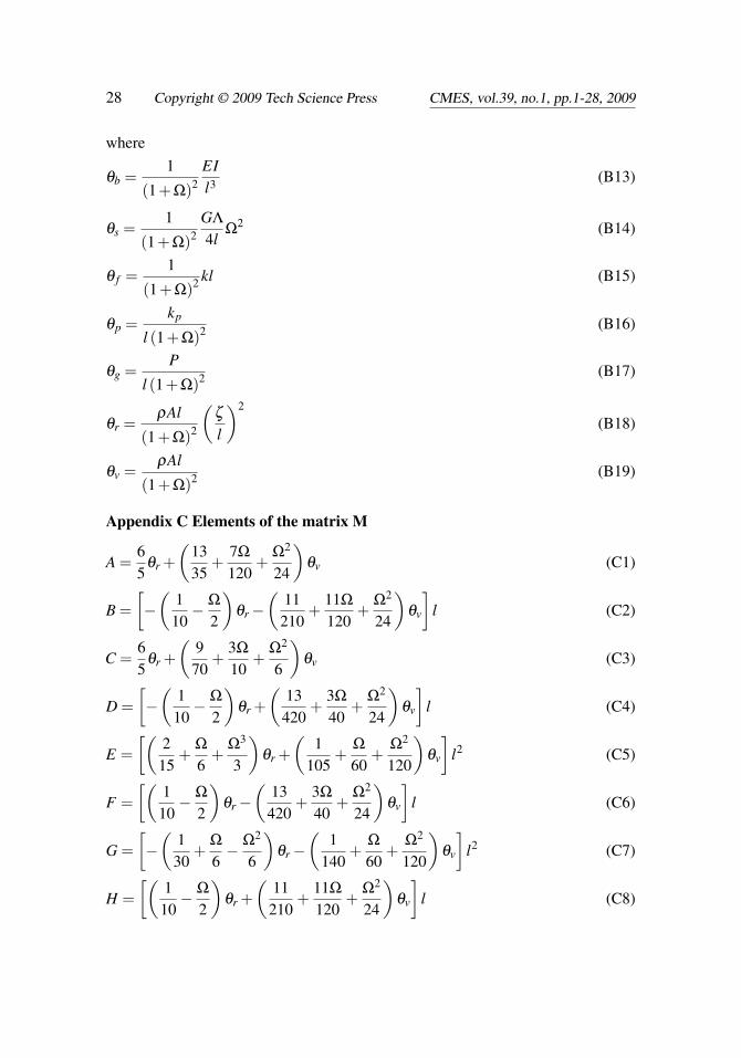
where

θb =1

(1+Ω)2EIl3 (B13)

θs =1

(1+Ω)2GΛ

4lΩ

2 (B14)

θ f =1

(1+Ω)2 kl (B15)

θp =kp

l (1+Ω)2 (B16)

θg =P

l (1+Ω)2 (B17)

θr =ρAl

(1+Ω)2

(ζ

l

)2

(B18)

θv =ρAl

(1+Ω)2 (B19)

Appendix C Elements of the matrix M

A =65

θr +(

1335

+7Ω

120+

Ω2

24

)θv (C1)

B =[−(

110− Ω

2

)θr−

(11210

+11Ω

120+

Ω2

24

)θv

]l (C2)

C =65

θr +(

970

+3Ω

10+

Ω2

6

)θv (C3)

D =[−(

110− Ω

2

)θr +

(13420

+3Ω

40+

Ω2

24

)θv

]l (C4)

E =[(

215

+Ω

6+

Ω3

3

)θr +

(1

105+

Ω

60+

Ω2

120

)θv

]l2 (C5)

F =[(

110− Ω

2

)θr−

(13420

+3Ω

40+

Ω2

24

)θv

]l (C6)

G =[−(

130

+Ω

6− Ω2

6

)θr−

(1

140+

Ω

60+

Ω2

120

)θv

]l2 (C7)

H =[(

110− Ω

2

)θr +

(11210

+11Ω

120+

Ω2

24

)θv

]l (C8)

Parameter identiﬁcation of beam-column structures on … · Parameter identiﬁcation of...

Documents

Transcript of Parameter identiﬁcation of beam-column structures on … · Parameter identiﬁcation of...