Identification of a Bipedal Robot with a Compliant

Drivetrain

Parameter estimation for control design

Hae-Won Park, Koushil Sreenath, Jonathan W. Hurst, and J.W.Grizzle

Research in bipedal robotics aims to design machines with the speed, stability, agility,

and energetic efficiency of a human. While no machine built today realizes the union of these

attributes, several robots demonstrate one or more of them.The Cornell Biped is designed to

be highly energy efficient [1]. This robot walks with a dimensionless mechanical-transport cost

cmt of 0.055; the corresponding efficiency for a typical human is0.05. The down side of this

achievement is that the robot can walk on only flat ground; it trips and falls in the presence

of ground variations of a few millimeters. The Planar Biped,which excels at agility, can run

stably on one or two legs, hop up and down stairs, and can boundover piles of blocks, but does

not walk well [2] [3] [4]. This robot is inefficient, due to itspneumatic and hydraulic actuation.

Moreover, the physical principles which underlie its mechanical design and its control system

are difficult to generalize to other machines. The bipedal robot Rabbit exhibits robustly stable

walking under model-based control [5], [6]; a controller implemented on the robot in 2002 still

functions today. On the other hand, Rabbit can run only a few steps without falling [7], and its

mechanical-transport cost is 0.38.

1

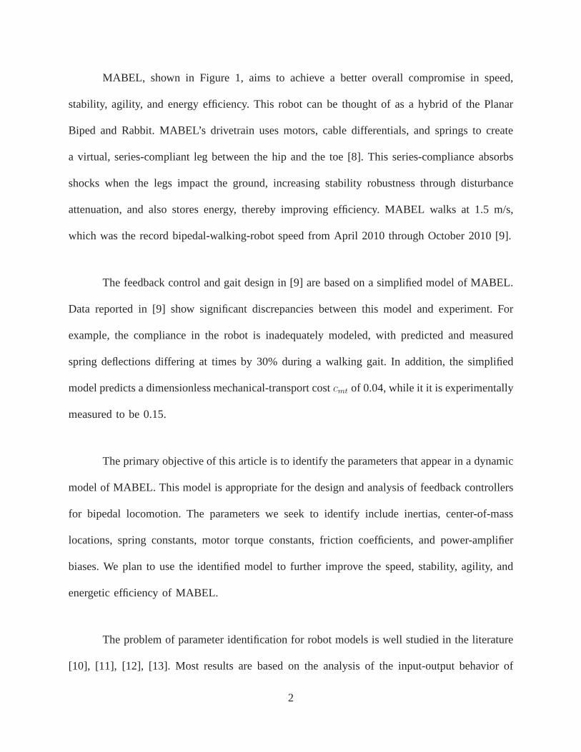
MABEL, shown in Figure 1, aims to achieve a better overall compromise in speed,

stability, agility, and energy efficiency. This robot can bethought of as a hybrid of the Planar

Biped and Rabbit. MABEL’s drivetrain uses motors, cable differentials, and springs to create

a virtual, series-compliant leg between the hip and the toe [8]. This series-compliance absorbs

shocks when the legs impact the ground, increasing stability robustness through disturbance

attenuation, and also stores energy, thereby improving efficiency. MABEL walks at 1.5 m/s,

which was the record bipedal-walking-robot speed from April 2010 through October 2010 [9].

The feedback control and gait design in [9] are based on a simplified model of MABEL.

Data reported in [9] show significant discrepancies betweenthis model and experiment. For

example, the compliance in the robot is inadequately modeled, with predicted and measured

spring deflections differing at times by 30% during a walkinggait. In addition, the simplified

model predicts a dimensionless mechanical-transport costcmt of 0.04, while it it is experimentally

measured to be 0.15.

The primary objective of this article is to identify the parameters that appear in a dynamic

model of MABEL. This model is appropriate for the design and analysis of feedback controllers

for bipedal locomotion. The parameters we seek to identify include inertias, center-of-mass

locations, spring constants, motor torque constants, friction coefficients, and power-amplifier

biases. We plan to use the identified model to further improvethe speed, stability, agility, and

energetic efficiency of MABEL.

The problem of parameter identification for robot models is well studied in the literature

[10], [11], [12], [13]. Most results are based on the analysis of the input-output behavior of

2

the robot during a planned motion, where the parameter values are obtained by minimizing the

difference between a function of the measured robot variables and the output of the model.

An illustration of this approach is presented in [11] for identifying parameters in industrial

manipulators. The standard rigid-body model is rewritten in the parametric formτ = φ(q, q, q)θ,

which is linear in the unknown parameters, whereq, q, q are the position, velocities, and

accelerations of the joints,τ is the vector of joint torques,θ is the unknown parameter vector,

and φ is the regressor matrix. Optimization is used to define trajectories that enhance the

condition number ofφ, and these trajectories are then executed on the robot. Weighted least-

squares estimation is applied to estimate the parameters, which in turn are validated by torque

prediction. This approach requires acceleration, which must be estimated numerically from

measured position.

An alternative approach explored in [12] uses force- and torque-sensor measurements

to avoid the need to estimate acceleration. The robot model is represented in Newton-Euler

form, and a six-element wrench at the robot’s wrist is expressed in a form that is linear in the

unknown parameters. Force and torque at the wrist are measured directly through force and

torque sensors, and parameter estimation is accomplished from this data without the need for

acceleration measurements. Another class of methods [13] uses an energy-based model that uses

velocity and position variables, but does not require acceleration. This method, however, relies

on the integration of the input torques and the joint velocities to compute energy, which is

problematic if the torque estimates are corrupted by an unknown bias.

Parameter identification for MABEL is a challenging task forseveral reasons. First,

3

MABEL has position encoders at the motors and joints, as wellas contact switches at the leg

ends, but lacks force and torque sensors. We thus use commanded motor torques as inputs

and motor and joint position encoders as outputs in order to extract model parameters. Due

to the quantization error of the encoders, it is difficult to estimate acceleration by numerically

differentiating encoder signals. Hence, we estimate parameters without calculating acceleration

from position data. Second, the actuator characteristics are poorly known. The motors used in

MABEL are brushless direct current (BLDC) motors, which arecustom manufactured on demand.

Due to the small production numbers, the rotor inertias and torque constants may differ by 20%

from the values supplied by the manufacturer. These parameters must therefore be included in

the identification procedure. In combination with power amplifiers from a second manufacturer,

the motors exhibit some directional bias. Complicating matters further, this bias varies among

individual amplifier-motor pairs. Consequently, the amplifier bias must be considered in the

identification process. A third issue affecting parameter identification is that the choice of exciting

trajectory is restricted due to limitations of MABEL’s workspace. For example, a constant-

velocity experiment for estimating friction coefficients is not feasible because the maximum

range of rotation of each joint is less than 180 deg. Finally,because MABEL has many degrees

of freedom, actuating all of them at once would require estimating 62 parameters simultaneously.

For this reason, we take advantage of the modular nature of the robot to design experiments that

allow us to sequentially build the model element by element,estimating only a few parameters

at each stage of the process.

M ECHANISM OVERVIEW

MABEL’s body consists of five links, namely, a torso, two thighs, and two shins. The

4

hip of the robot is attached to a boom, as shown in Figure 2. Therobot’s motion is therefore

tangent to a sphere centered at the pivot point of the boom on the central tower. The boom is

2.25 m long, and while the resulting walking motion of the robot is circular, it approximates the

motion of a planar biped walking along a straight line.

The actuated degrees of freedom of each leg do not correspondto the knee and the hip

angles as in a conventional biped. Instead, as shown in figures 3 and 4, for each leg, a collection

of differentials is used to connect two motors to the hip and knee joints in such a way that one

motor controls the angle of the virtual leg defined by the lineconnecting the hip to the toe, while

the second motor is connected in series with a spring to control the length of the virtual leg.

Conventional bipedal robot coordinates and MABEL’s actuated coordinates, which are depicted

in Figure 4, are related by

qLA =1

2(qTh + qSh) (1)

and

qLS =1

2(qTh − qSh) , (2)

whereLA stands for leg angle,LS stands for leg shape,Th stands for thigh, andSh stands for

shin.

The springs in MABEL isolate the leg-shape motors from the impact forces at leg

touchdown. In addition, the springs store energy during thecompression phase of a running

gait, when the support leg must decelerate the downward motion of the robot’s center of mass.

The energy stored in the spring can then be used to redirect the center of mass upwards for

the subsequent flight phase, propelling the robot off the ground. As explained in [14], [15],

5

[16], both of these properties, shock isolation and energy storage, enhance the energy efficiency

of running and reduce the actuator power requirements. Similar advantages are also present in

walking on flat ground, but to a lesser extent compared to running on uneven terrain, due to the

lower forces at leg impact and the reduced vertical travel ofthe center of mass. The robotics

literature strongly suggests that shock isolation and compliance are useful for walking on uneven

terrain [17], [18], [19], [20], [21], [22], [23].

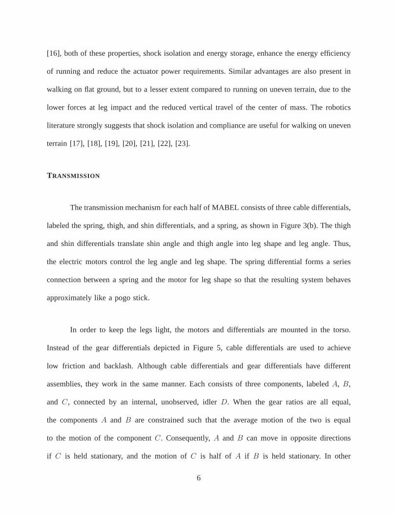
TRANSMISSION

The transmission mechanism for each half of MABEL consists of three cable differentials,

labeled the spring, thigh, and shin differentials, and a spring, as shown in Figure 3(b). The thigh

and shin differentials translate shin angle and thigh angleinto leg shape and leg angle. Thus,

the electric motors control the leg angle and leg shape. The spring differential forms a series

connection between a spring and the motor for leg shape so that the resulting system behaves

approximately like a pogo stick.

In order to keep the legs light, the motors and differentialsare mounted in the torso.

Instead of the gear differentials depicted in Figure 5, cable differentials are used to achieve

low friction and backlash. Although cable differentials and gear differentials have different

assemblies, they work in the same manner. Each consists of three components, labeledA, B,

and C, connected by an internal, unobserved, idlerD. When the gear ratios are all equal,

the componentsA and B are constrained such that the average motion of the two is equal

to the motion of the componentC. Consequently,A and B can move in opposite directions

if C is held stationary, and the motion ofC is half of A if B is held stationary. In other

6

words,(qA + qB)/2 = qC and (qA − qB)/2 = qD, whereqA, qB, qC , andqD denote the angular

displacements of the components.

In MABEL’s transmission mechanism,A andB are inputs to the differential, whileC

is an output. In the following,AShin, BShin and CShin refer to the componentsA, B, andC

of the shin differential and likewise for the remaining two differentials.CThigh and CShin in

Figure 3(b) are attached to the thigh and shin links, respectively. The pulleysBThigh andBShin

are both connected to the leg-angle motor. The pulleysAThigh andAShin are connected to the

pulley CSpring, which is the output pulley of the spring differential. The spring on each side

of the robot is implemented with two fiberglass plates connected in parallel to the differentials

through cables, as shown in Figure 1. Due to the cables, the springs are unilateral, meaning they

can compress but not extend; this aspect is discussed below.

Figures 6 and 7 illustrate how this transmission works when one of the coordinatesqLA

or qLS is actuated, while the other coordinate is held fixed. The path from spring displacement

to rotation inqLS is similar. The net motion inqLS from the leg-shape motor and the spring is

the sum of the individual motions.

VARIABLE NAMES

To name the variables appearing in the robot, we use the indexset

I = {mLSL, mLAL, mLSR, mLAR}, (3)

where the subscriptsL andR mean left and right,mLS means motor leg shape, andmLA means

7

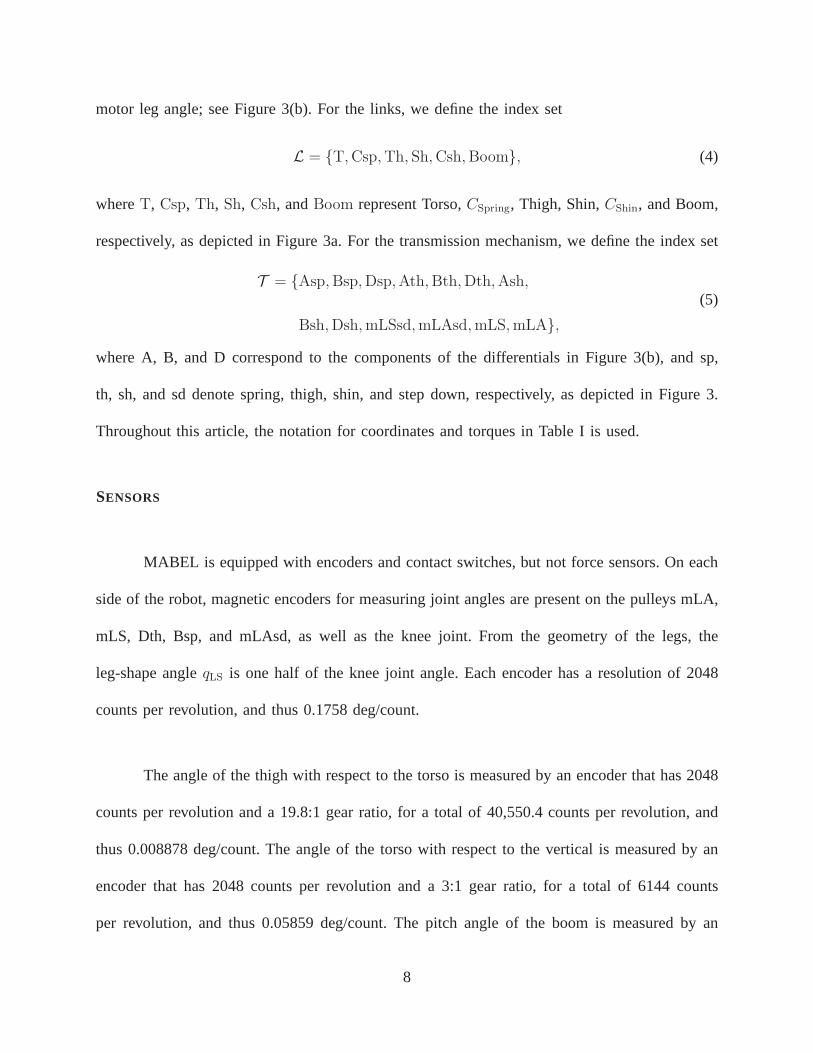
motor leg angle; see Figure 3(b). For the links, we define the index set

L = {T,Csp,Th, Sh,Csh,Boom}, (4)

whereT, Csp, Th, Sh, Csh, andBoom represent Torso,CSpring, Thigh, Shin,CShin, and Boom,

respectively, as depicted in Figure 3a. For the transmission mechanism, we define the index set

T = {Asp,Bsp,Dsp,Ath,Bth,Dth,Ash,

Bsh,Dsh,mLSsd,mLAsd,mLS,mLA},

(5)

where A, B, and D correspond to the components of the differentials in Figure 3(b), and sp,

th, sh, and sd denote spring, thigh, shin, and step down, respectively, as depicted in Figure 3.

Throughout this article, the notation for coordinates and torques in Table I is used.

SENSORS

MABEL is equipped with encoders and contact switches, but not force sensors. On each

side of the robot, magnetic encoders for measuring joint angles are present on the pulleys mLA,

mLS, Dth, Bsp, and mLAsd, as well as the knee joint. From the geometry of the legs, the

leg-shape angleqLS is one half of the knee joint angle. Each encoder has a resolution of 2048

counts per revolution, and thus 0.1758 deg/count.

The angle of the thigh with respect to the torso is measured byan encoder that has 2048

counts per revolution and a 19.8:1 gear ratio, for a total of 40,550.4 counts per revolution, and

thus 0.008878 deg/count. The angle of the torso with respectto the vertical is measured by an

encoder that has 2048 counts per revolution and a 3:1 gear ratio, for a total of 6144 counts

per revolution, and thus 0.05859 deg/count. The pitch angleof the boom is measured by an

8

encoder with 2048 counts per revolution and a 17.6:1 gear ratio, for a total of 36,044.8 counts

per revolution, and thus 0.09988 deg/count. The rotation angle of the central tower is measured

by an encoder with 40,000 counts per revolution and a 7.3987:1 gear ratio, for a total of 295,948

counts per revolution, and thus 0.001216 deg/count.

To detect impacts with the ground, two contact switches are installed at the end of

each leg. Ground contact is declared when either of the two switches closes. Additional contact

switches are installed at the hard stops on various pulleys to detect excessive rotation within

MABEL’s workspace. If a contact switch on a hard stop closes,power to the robot is immediately

turned off by the computer.

Because MABEL does not have velocity sensors, angular velocities must be estimated by

numerically differentiating position signals. For real-time applications, such as feedback control,

causal methods for numerical differentiation are required[24], [25]. For offline applications,

such as parameter identification, acausal or smoothing algorithms can be employed [26]. We use

the spline interpolation method of [27], which can be used ina causal or acausal manner.

EMBEDDED COMPUTER AND DATA ACQUISITION

The onboard computer is a 1.3-GHz Intel Celeron M CPU runninga QNX real-time

operating system. The RHexLib library, originally developed for the robot RHex [28], is used

for implementing control-algorithm modules as well as for logging data over the network data and

communicating with the robot. A user interface for monitoring the robot’s state on a secondary

Linux-based system uses utilities provided by RHexLib.

9

Digital and analog IO are handled with compactPCI data-acquisition cards from Acromag.

A custom-built compactPCI module houses the interface circuitry between the Acromag data-

acquisition cards and the sensors on the robot.

The sample period of the embedded controller is set at 1 ms. Though a 1.5 ms sample

period is probably adequate, the power to the robot is automatically shut off by a watchdog

timer if any controller update cycle exceeds 1 ms. Data acquisition and logging consume

approximately 0.5 ms of each sample period, leaving 0.5 ms for control computations and

signal processing. PD-based controllers can be implemented in the available processing time

without special programming considerations. For controllers based on inverse dynamics, such as

those reported in [9], the real-time calculations are performed in approximately 0.11 ms with

a public-domain C++-template library from Boost [29], which provides standard matrix-algebra

operations.

PARAMETER I DENTIFICATION PROCEDURE

CAD packages provide estimates of the masses of the links andpulleys comprising

MABEL, their lengths and radii, centers of mass, and momentsof inertia. If we also account for

the location and mass distribution of items not normally represented in a CAD drawing, such as

ball bearing shape and density, the length and density of pulley cables, electrical wiring, onboard

power electronics, and actuators and sensors, then the mechanical parameters of the robot can be

estimated. Consequently, one goal of the identification procedure is to validate these estimates

by comparing predicted responses to experimental data.

In addition, model parameters for which reliable estimatesare not available from

10

CAD drawings include motor torque constants, rotor inertias, spring stiffness, and pre-load.

Finally, friction parameters cannot be estimated by a CAD program and must be determined

experimentally. The parameters to be identified are shown inTable II.

STEPS IN THE I DENTIFICATION PROCESS

The first phase of the identification process focuses on estimating the actuator parameters

and the friction parameters in the transmission, as well as validating the pulley inertia estimates

provided by the CAD program. The torque constantKT and rotor inertiaJrotor of each motor

are also determined by analyzing the motors in series with a chain of known inertias formed by

selectively coupling the pulleys that form the three differentials, as shown in figures 6 and 7.

Because the pulleys are connected by low-stretch steel cables to form a one-degree-of-freedom

system, various paths in the transmission mechanism can be modeled by lumping the moments

of inertia of the pulleys. This lumped moment of inertia can be calculated by the CAD model

and added to the rotor inertia of the motor. In addition, thislumped moment of inertia can be

obtained from experiments. These data can be used to estimate motor torque constants, rotor

inertias, viscous friction, and motor torque biases.

Next, the legs are coupled to the transmission to validate the actuation-transmission model

in conjunction with the center of mass and moments of inertias of the links constituting the thigh

and shin, as provided by the CAD model. For these experiments, the compliance is removed from

the system by locking the orientation of the pulleyBSpring; the torso is held in a fixed position

as well. Following this experiment, the torso’s inertial parameters are estimated for validation.

11

Compliances are determined last. Two sources of complianceare present in the robot.

One source is the unilateral, fiberglass spring designed into the transmission. The other source,

which is unplanned, arises from stretching of the cables between the pulleys. The compliance

of the unilateral spring is obtained from static experiments, and the compliance due to cable

stretch is estimated from dynamic experiments that apply high torques to the robot.

EXPERIMENTAL SETUP FOR THE M OTOR , DIFFERENTIAL , AND L EG PARAMETERS

The first phase of the identification process uses the setup depicted in Figure 8. The

torso is fixed relative to the world frame, and the legs can freely move. The position of the

pulley BSpring is fixed as well, removing compliance for the initial identification phase. Torque

commands are recorded and sent to the amplifiers. In turn, theamplifiers regulate the currents

in the motor windings, thereby setting the motor torque values. The rotation of the motors

is transmitted to the thigh and shin links through the transmission differentials as shown in

figures 6, 7, and 8.

The leg anglesqLA andqLS are related to the corresponding motor angles and the angle

of the pulleyBSpring by

qLA =1

γLA→mLA

qmLA (6)

and

qLS =1

γLS→mLS

qmLS +1

γLS→Bsp

qBsp, (7)

whereγLS→mLS = 31.42, γLA→mLA = −23.53, andγLS→Bsp = 5.18 are the gear ratios fromLS to

mLS, from LA to mLA, and fromLS to Bsp. The calculated anglesqLS andqLA are also logged

12

during the experiments.

The relations (6) and (7) hold under the assumption that the cables do not stretch, which

is the approximation made here, because no external loads are applied to the legs or the pulleys.

When the robot is walking, the transmission system is heavily loaded due to the weight of the

robot, and cable stretching occurs. This behavior is observed by the violation of the relations

(6) and (7). Cable stretch is taken into account in the last step of the identification process.

It is typical for power amplifiers to exhibit a small bias in the commanded current, which

in turn causes bias in the motor torques. Before beginning system identification, these biases

are estimated and compensated for each motor following the procedure described in “How to

Estimate Motor-Torque Biases”.

TRANSMISSION I DENTIFICATION

For system identification, the fact that the differentials in the transmission are realized

by a series of cables and pulleys is an advantage because we can select how many pulleys are

actuated by disconnecting cables. For each pulley combination, the lumped moment of inertia

can be computed. Therefore, if the electrical dynamics of the motor and power amplifiers are

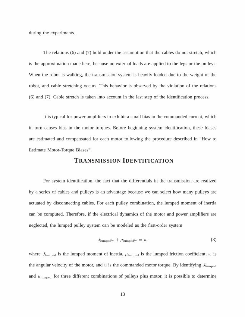
neglected, the lumped pulley system can be modeled as the first-order system

Jlumpedω + µlumpedω = u, (8)

whereJlumped is the lumped moment of inertia,µlumped is the lumped friction coefficient,ω is

the angular velocity of the motor, andu is the commanded motor torque. By identifyingJlumped

andµlumped for three different combinations of pulleys plus motor, it is possible to determine

13

KT andJrotor, as well as confirm the lumped pulley inertia predicted by theCAD model. For

each side of the robot, the three pulley combinations of Figure 9(a) are used for the leg-angle

path, while the three pulley combinations of Figure 9(b) areused for the leg-shape path.

M OTOR TORQUE CORRECTION FACTOR AND I NERTIA CORRECTION FACTOR

The leg-angle-identification experiments are performed successively on the leg-angle

motor in combination with one, three, and five pulleys as shown in Figure 9(a). The leg-shape-

identification experiments are performed successively on the leg-shape motor in combination

with one, three, and five pulleys as shown in Figure 9(b). The lumped moments of inertia of

each combination, including the contributions of the cables can be expressed as

Ji = Jrotor + Jpulley,i + Jcable,i, i = 1, 2, 3, (9)

wherei denotes experiment number,Jrotor is the inertia of the motor rotor,Jpulley,i is the lumped

moment of inertia of the pulley combination for experimenti, which is obtained by combining

the pulley inertias shown in Table III with the gear ratios between the pulleys taken into account,

andJcable,i is the lumped cable moment of inertia calculated from the mass of the cable per unit

length and the length of the cable, with gear ratios taken into account.

Letting Jrotor,man denote the value of the rotor inertia supplied by the manufacturer, we

define the scale factorαrotor by

αrotor =Jrotor

Jrotor,man

, (10)

which we seek to estimate. In a similar manner, we define the scale factorαtorque for the motor

14

by

αtorque =KT

KT,man

, (11)

whereKT,man is the value of the motor torque constant supplied by the manufacturer andKT is

the true motor torque constant. In each experiment, the commanded motor torque is calculated by

multiplying the current commanded by the power amplifier byKT,man. As illustrated in Figure 10,

it follows that the transfer function from the commanded motor torque to the measured motor

angular velocity is a scalar multiple of (8). Hence, the moment of inertia from the experiments

is related to the moment of inertia of (9) by

Jexp,i = αtorque(αrotorJrotor,man + Jpulley,i + Jcable,i), i = 1, 2, 3, (12)

whereJexp,i is the lumped moment of inertia estimated on the basis of theith experiment.

Three moment of inertia estimates, denoted byJexp,1, Jexp,2, andJexp,3 respectively, are

obtained from each of the leg-shape and leg-angle experiments. Arranging the equations for each

set of experiments in matrix form gives

Ψ = Γ

αtorqueαrotor

αtorque

, (13)

where

Ψ =

Jexp,1

Jexp,2

Jexp,3

, Γ =

Jrotor,man Jpulley,1 + Jcable,1

Jrotor,man Jpulley,2 + Jcable,2

Jrotor,man Jpulley,3 + Jcable,3

.

15

The estimates ofαtorque andαrotor are then obtained by least squares fit

αtorqueαrotor

αtorque

, (ΓTΓ)−1ΓTΨ. (14)

EXPERIMENTAL RESULTS

Inputs for identification are designed as follows. Startingfrom 0.5 Hz, the input frequency

is increased in 17 steps to 50 Hz. To allow the system responseto reach steady state, each

frequency is held constant for 10 periods until changing to the next higher frequency. At each

frequency increment, the magnitude is also incremented to prevent the measured motor angular

velocity from becoming too small. Figure 11 illustrates theinput signal and corresponding system

response. The Matlab System Identification Toolbox is used to identify the transfer function (8).

Table IV shows the results obtained from the experiments.

On the basis of the values in Table IV,αtorque and αrotor are calculated by (14).

The estimated values are listed in Table V, along with the motor biases. The scale factors

αrotor indicate that the actual rotor inertias of the leg-shape motors are within 7% of the

manufacturer’s reported values, while the rotor inertias of the leg-angle motors are 25% less

than the manufacturer’s reported values. The scale factorsαtorque of the leg-angle motors on

the left and right sides of the robot differ by less than 5%. For the leg-shape motors, the large

difference in the scale factorsαtorque is expected. In particular, motors of different characteristics

for the left and right sides of the robot was necessary when one of the motors failed early in the

construction process and was replaced with a motor from a previous prototype. We also note

16

that motor biases, which range in magnitude from 0.002 to 0.107 N-m, are small in comparison

to the torques that are expected in walking experiments, which can exceed 2 N-m for leg angle

and 8 N-m for leg shape [9].

For the remainder of this article, the motor torque constantis computed by

KT = αtorqueKT,man.

L EG AND TORSO PARAMETERS

THIGH AND SHIN L INKS

The thigh and shin links of the legs are actuated by the torquetransmitted through the

transmission, as shown in figures 3(b) and 8. The total mass, center of mass, and inertia of each

link are assumed known from the CAD model; their values are given in Table VI. The values of

the motor torque constants and rotor inertias estimated forthe transmission are assumed. Friction

coefficients may differ from the values estimated for the transmission, however, because the hip

and knee joints are now actuated. In this section, the torso continues to be fixed relative to the

world frame and the position of the pulleyBSpring is fixed as well, removing compliance from

the picture.

With the torso fixed, the left and right sides of the robot are,in principle, decoupled; in

practice, some coupling of vibration from one side to the other occurs because the test stand is

not perfectly rigid, but this coupling is ignored. Choosingthe coordinatesq = (qmLA, qmLS)T ,

17

the dynamic model for each side can be written in the form

D(θ, αrotor, q)q + C(θ, αrotor, q, q)q +G(θ, αrotor, q) = ΓQ, (15)

whereD(θ, αrotor, q), C(θ, αrotor, q, q), andG(θ, αrotor, q) are the inertia matrix, Coriolis matrix,

and gravity vector, respectively. Moreover,θ is the vector of mechanical parameters from the

CAD model, the rotor inertia correction factorsαrotor are from Table V, and the vectorΓQ of

generalized forces acting on the robot, consisting of motortorque and viscous friction, is given

by

ΓQ = umLA + umLS − µmLAqmLA − µmLSqmLS. (16)

The friction coefficientsµmLA andµmLS are to be estimated.

Two types of experiment are performed, SISO and MIMO. Each experiment is performed

on one leg at a time. In the SISO experiments, one degree of freedom is actuated and logged,

either qmLS or qmLA, while the other degree of freedom is mechanically locked. In the MIMO

experiment, bothqmLS andqmLA are actuated and recorded. The objective of the SISO experiments

is to estimate the friction parameters in (16). The objective of the MIMO experiment is to validate

the model (15), with the parameters obtained from the SISO experiment.

The commanded motor torque is a modified chirp signal plus a constant offset, similar to

the transmission identification experiments. The magnitude and offset of the input signal must

be selected to keep the links within the robot’s work space.

With all the parameters in the model (15) specified, the response of the system excited

by the input used in the experiments can be simulated, as shown in Figure 12. The friction

18

parametersµ are estimated by minimizing the cost function

J(µ) =√

∑

(yexp − ysim(µ)), (17)

whereyexp is the vector of experimentally measured data,ysim is the vector of simulated data,

and µ is the vector of viscous-friction coefficients. As shown in Table VII, the values ofµ

estimated in this manner are larger than the values from the transmission experiments, but not

greatly different from those values.

In the MIMO simulations, we observe that variations in the assumed actuator bias of 0.1

N-m, which can be ignored when the legs are supporting the robot, can cause large deviations

in the system response when the legs are not supporting the robot. Therefore, for the MIMO

simulations, in place of the bias values estimated from the transmission identification, we use

the values that minimize the cost function

J(b) =√

∑

(yexp − ysim(b)), (18)

whereyexp is the vector of experimentally measured data,ysim is the vector of simulated data,

and b is the bias vector.

The comparisons between simulated and experimental results are presented in figures 13

and 14. All figures showqLS and qLA computed fromqmLS and qmLA, because the body

coordinatesqLS and qLA are easier to interpret than the motor positions. It is emphasized that

the parameters are either from the transmission identification experiments or the CAD model,

with two exceptions, namely, friction is estimated in the SISO experiments from (17) and used

in the MIMO experiments; in the MIMO experiments, motor biases are tuned by (18).

19

In the SISO experiments, the RMS error varies from 0.69 to 1.1deg, while for the MIMO

experiments, the RMS error varies from 0.72 to 1.42 deg. These errors may arise from several

sources. For example, the linear viscous-friction terms in(16), namelyµmLA qmLA andµmLS qmLS,

do not take into account stick-slip behavior in the low-velocity region. Furthermore, electrical

wiring is not included in calculating inertial parameters.In addition, motor bias changes slightly

for each experimental trial. Finally, cable stretch is assumed to be negligible.

TORSO

The torso represents approximately 41 kg of the total 65-kg mass of the robot.

Consequently, the mass and inertia of the torso strongly affect the dynamics of the robot. In

principle, the inertia and mass distribution of the torso can be validated by locking the legs in a

fixed position, and using the leg-angle motors to oscillate the torso. Attempts at executing this

experiment in the test stand failed, since movement of the torso is always translated to the legs.

Therefore, instead of dynamic identification of the torso, static balancing experiments are

used to validate the CAD model estimates. In the first experiments, the robot is not constrained.

Using local PD controllers, we command a posture where the right leg is extended more than

the left leg. The robot is then balanced by hand on the right leg. The balance of the robot is

maintained with minimal fingertip pressure from one of the experimenters. Once the robot is in a

balanced posture, the joint position data are recorded. Many different postures are balanced and

logged. From the logged data, we calculate the center of massposition of the robot including the

horizonal boom, and we verify that the calculated center of mass is located over the supporting

toe.

20

In a second set of experiments, the position of the hip joint is fixed, with the legs hanging

below the robot and above the floor, and with the robot unpowered. The torso is balanced by

hand in the upright position. We then calculate the center ofmass position of the robot without

the boom, and check that the center of mass is aligned over thehip joint.

We use 10 different postures for the first experiment and 7 different postures for the second

experiment. Figure 15(a) displays the horizontal distancebetween the center of mass and the

supporting toe for the first experiment, and Figure 15(b) shows the horizontal distance between

the center of mass and the hip for the second experiment. We observe that the maximum error is

6 mm, which is negligible in view of the size of the robot and considering that the experiments

are performed with manual balancing. These experiments do not provide information on the

vertical position of the center of mass.

COMPLIANCE

The stiffness of the springs that are in series with the leg-shape actuators is estimated by

means of static experiments using the calculated spring torques and measured spring deflections.

The magnitude of the joint torques used in these experimentsis more representative of the

torques used in walking [9]. Under these greater loads, the cables in the differentials stretch.

This compliance is also modeled.

SPRING STIFFNESS

The series compliance in the drivetrain is now estimated by means of static, constant-

torque experiments, performed by balancing the robot on oneleg at a time. The setup is illustrated

21

in Figure 16. In these experiments, the torso is no longer locked in place relative to the world

frame; it is free. The actuators on one side of the robot are disabled, with the leg on that side

folded and tied to the torso. On the other side, a PD-controller is used to maintain the leg angle

at 180 deg, which is straight down. A second PD-controller isused to set the nominal leg shape.

An experimenter balances the robot in place with the toe resting on a scale placed on the floor;

the experimenter adjusts the overall angle of the robot so that it is exactly balanced on the toe,

as when verifying the center of mass of the torso.

With the setup shown in Figure 16, the scale is measuring the combined weight of the

robot and the boom. By the design of the differential, when the leg-shape motor holds the pulley

ASpring in a fixed orientation, the torque at the pulleyCSpring is exactly balanced by the torque at

the pulleyBSpring. The torqueτgravity at CSpring, shown in Figure 16, is the weight of the robot

transmitted through the thigh and shin differentials; its magnitude is given by

|τgravity| =

∣

∣

∣

∣

1

2Wrobot sin(qLS)

∣

∣

∣

∣

, (19)

whereWrobot is the weight of the robot measured by the scale at the bottom of the foot. The

absolute value is used because spring stiffness is positive. The torqueτBsp at the pulleyBSpring,

shown in Figure 16, is due to the deflection of the spring and isgiven by

τBsp = KBqBsp, (20)

whereKB is the spring stiffness. The spring deflectionqBsp is measured by an encoder installed in

the pulleyBSpring. The torquesτgravity andτBsp, which are related by the differential mechanism,

satisfy

|τgravity| = 2.59 |τBsp| . (21)

22

Combining (19), (20), and (21), the spring stiffness is obtained as

KB =1

5.18

∣

∣

∣

∣

Wrobot sin(qLS)

qBsp

∣

∣

∣

∣

. (22)

The design of the experiment is completed by varyingqLS over a range of values, here

taken to be from 10 deg to 30 deg. We emphasize thatKB determined by means of (22) does

not depend on the estimated leg-shape motor torque. Indeed,because the spring and motor are

connected in series, the torques must balance at the spring differential.

Figure 17 shows the results of performing the above experiments on each leg. Prior to

the experiments, it is not obvious if a linear model of the spring deflection would be adequate

because the spring folds around the curved torso as shown in Figure 18. From the data, we

observe that the spring behavior is nearly linear, and that the spring constants for the left and

right sides are consistent.

CABLE STRETCH

Experiments reported in [9] show that the cables used in the differentials of MABEL

stretch a significant amount under loads typical of bipedal walking. This compliance breaks the

relations in (6) and (7). Consequently,qLA andqmLA are independent degrees of freedom, as are

qLS, qmLS, andqBsp.

We take into account the stretching of the cables with a spring-damper model. First, the

23

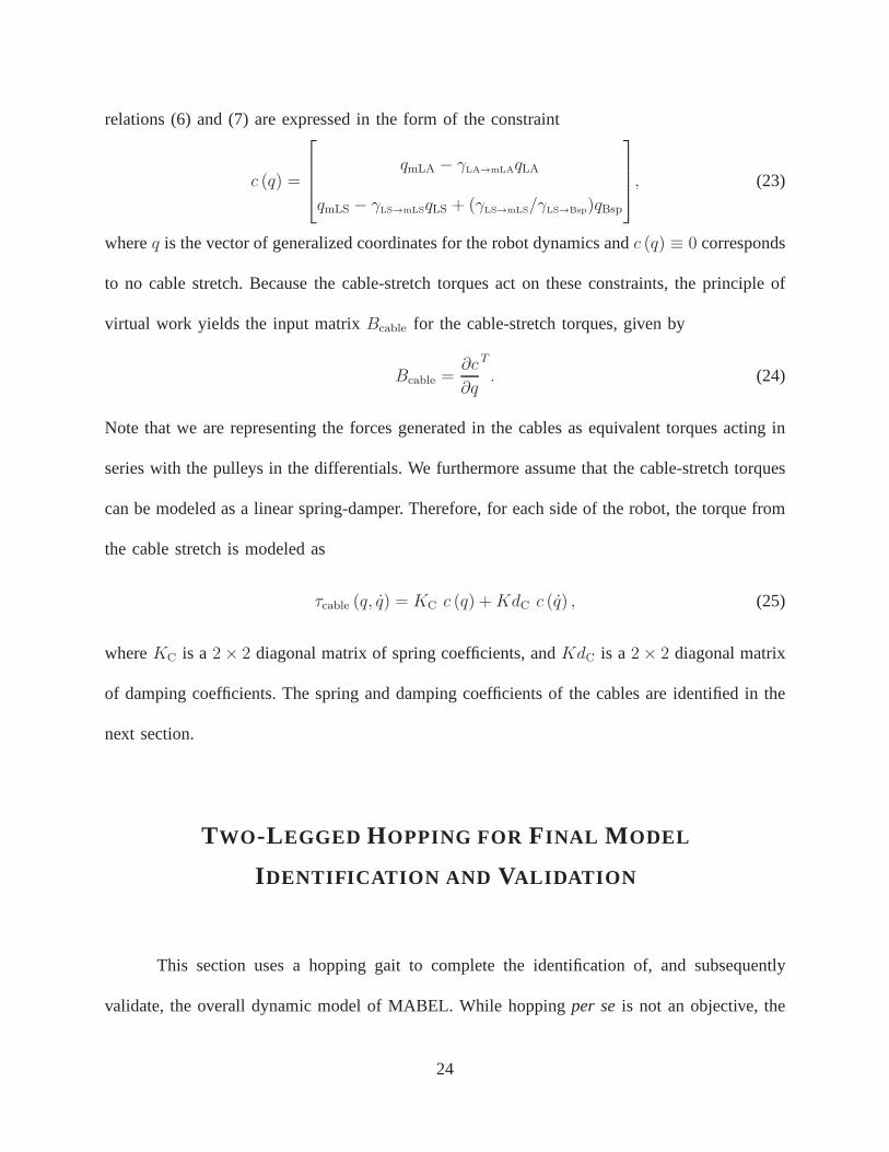
relations (6) and (7) are expressed in the form of the constraint

c (q) =

qmLA − γLA→mLAqLA

qmLS − γLS→mLSqLS + (γLS→mLS/γLS→Bsp)qBsp

, (23)

whereq is the vector of generalized coordinates for the robot dynamics andc (q) ≡ 0 corresponds

to no cable stretch. Because the cable-stretch torques act on these constraints, the principle of

virtual work yields the input matrixBcable for the cable-stretch torques, given by

Bcable =∂c

∂q

T

. (24)

Note that we are representing the forces generated in the cables as equivalent torques acting in

series with the pulleys in the differentials. We furthermore assume that the cable-stretch torques

can be modeled as a linear spring-damper. Therefore, for each side of the robot, the torque from

the cable stretch is modeled as

τcable (q, q) = KC c (q) +KdC c (q) , (25)

whereKC is a 2× 2 diagonal matrix of spring coefficients, andKdC is a2× 2 diagonal matrix

of damping coefficients. The spring and damping coefficientsof the cables are identified in the

next section.

TWO -L EGGED HOPPING FOR FINAL M ODEL

I DENTIFICATION AND VALIDATION

This section uses a hopping gait to complete the identification of, and subsequently

validate, the overall dynamic model of MABEL. While hoppingper seis not an objective, the

24

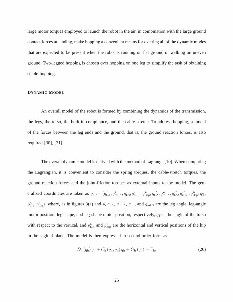
large motor torques employed to launch the robot in the air, in combination with the large ground

contact forces at landing, make hopping a convenient means for exciting all of the dynamic modes

that are expected to be present when the robot is running on flat ground or walking on uneven

ground. Two-legged hopping is chosen over hopping on one legto simplify the task of obtaining

stable hopping.

DYNAMIC M ODEL

An overall model of the robot is formed by combining the dynamics of the transmission,

the legs, the torso, the built-in compliance, and the cable stretch. To address hopping, a model

of the forces between the leg ends and the ground, that is, theground reaction forces, is also

required [30], [31].

The overall dynamic model is derived with the method of Lagrange [10]. When computing

the Lagrangian, it is convenient to consider the spring torques, the cable-stretch torques, the

ground reaction forces and the joint-friction torques as external inputs to the model. The gen-

eralized coordinates are taken asqh := (qLLA; qLmLA; q

LLS; q

LmLS; q

LBsp; q

RLA; q

RmLA; q

RLS; q

RmLS; q

RBsp; qT;

phhip; pvhip), where, as in figures 3(a) and 4,qLA, qmLA, qLS, andqmLS are the leg angle, leg-angle

motor position, leg shape, and leg-shape motor position, respectively,qT is the angle of the torso

with respect to the vertical, andphhip andpvhip are the horizontal and vertical positions of the hip

in the sagittal plane. The model is then expressed in second-order form as

Dh (qh) qh + Ch (qh, qh) qh +Gh (qh) = Γh, (26)

25

where the vector of generalized forces and torquesΓh acting on the robot is given by

Γh = Bhu+Bfricτfric (qh, qh) +BspτBsp (qh, qh) +

∂ptoe∂qh

T

F +Bcableτcable (qh, qh) .

(27)

Here,ptoe is the position vector of the two leg ends,F is the ground reaction forces on the two

legs, and the matricesBh, Bfric, Bsp, andBcable, which are derived from the principle of virtual

work, define how the actuator torquesτ , the joint friction torquesτfric, the spring torquesτBsp,

and the cable-stretch torquesτcable enter the model, respectively.

The model for the unilateral spring is augmented with terms to represent the hard stop,

yielding

τBsp =

−KBqBsp −KdBqBsp, qBsp > 0,

−KBqBsp −Kd1q3Bsp −Kvd1qBsp, qBsp ≤ 0 and qBsp ≥ 0,

−KBqBsp −Kd1q3Bsp −Kvd1qBsp

−Kvd2

√

|qBsp|sgn(qBsp), qBsp ≤ 0 and qBsp < 0,

(28)

whereKB corresponds to the spring constants determined in Figure 17, and where the remaining

parametersKdB, Kd1, Kvd1, andKvd2 are to be estimated from hopping data. WhenqBsp > 0,

the spring is deflected and the model is a linear spring-damper. When qBsp ≤ 0, the pulley is

against the hard stop, a stiff damper. This model captures the unilateral nature of MABEL’s

built-in compliance.

The ground reaction forces at the leg ends are based on the compliant ground model in

[30], [31], using the modifications presented in [32]. The normal forceFn and tangential force

Ft acting on the end of each leg are determined by

26

Fn = −λav|zG|

nzG − λbv|zG|

nsgn(zG)√

|zG|+ k|zG|n, (29)

Ft = µ(d, v)|Fn|, (30)

where

d = v − |v|σh0

αh0

d, (31)

µ(d, v) = σh0d+ σh1d+ αh2v, (32)

when the penetration depthzG of a leg into the ground is positive, and are zero otherwise.

The normal forceFn corresponds to a nonlinear spring-damper, with damping coefficient λav

and spring stiffnesskv. According to [30], the exponentn, which depends on the shapes of the

surfaces that are in contact, equals1.5 when the leg end is spherical, which is roughly the case

for MABEL. The signed-square-root term on penetration velocity, with coefficientλbv, induces

finite-time convergence of the ground penetration depth when the robot is standing still.

The tangential forceFt is in the form of a friction model with variable coefficient of

friction µ determined by the LuGre model [31]. The LuGre model represents the interface

between the two contacting surfaces as bristles, modeled bysprings and dampers, which, if the

applied tangential force is sufficient, are deflecting and slipping. The average deflectiond of

the bristles is the internal state of the friction model,v is the relative velocity of the contacting

surfaces,σh1 is the damping coefficient, andσh2 is the coefficient of viscous friction. The stiffness

of the spring isσh0 and the coefficient of static friction isαh0.

PARAMETERS FOR CABLE STRETCH , HARD STOP, AND GROUND M ODELS

27

A heuristic controller for a hopping gait is given in “How Hopping is Achieved.” Because

the cable stretch coefficients are not yet identified, the hopping controller is hand tuned on an

approximate simulation model that assumes the cables are rigid; the approximate model also

uses the ground reaction parameters from [32]. The tuning process adjusts PD-controller gains

and setpoints in the various phases of the gait, with the goalof obtaining sustained hopping.

When the controller is implemented on MABEL, steady-state hopping is not achieved, even after

extensive trial-and-error tuning in the laboratory. Five hops is typical before the robot falls.

Even though sustained hopping is not achieved, the data fromthe experiments can

be used to identify the parameters in the hard-stop model, the cable stretch model, and the

compliant-ground-contact model. The parameter fitting is accomplished with a combination of

hand adjustment and nonlinear least squares. The resultingparameters are given in Table VIII.

Plots demonstrating the closeness of fit of the model to the identification data are not shown for

reasons of space. Instead, validation data is reported.

HOPPING EXPERIMENTS FOR VALIDATION

When the nominal hopping controller is simulated on the identified model, the closed-

loop system is found to be unstable. Event-based updates to the torso angle are therefore added

to achieve stability, as explained in “How Hopping is Achieved.” The controller is then applied

to MABEL, resulting in 92 hops before the test is deliberately terminated. The data are presented

next.

Figures 19 - 22 compare typical experimental results against the simulation results for

28

the 31st and 32nd hops. Figures 19 and 20 depict joint position angles. It is observed that the

period of the experimental data is longer than that of the simulation results by approximately

30 ms. Because the hopping controller regulates four outputs computed fromqT, qLAL, qLAR

,

qmLAL, andqmLAR

, it could be argued that the closeness of the simulated and experimental values

is a reflection of the controller. However, the spring compressionsqBspL and qBspR , as well as

the horizontal and vertical hip positionsphhip andpvhip, are unregulated, and Figure 20 shows that

these variables are captured by the model.

Figure 21 depicts joint torques. The simulation predicts the joint torques observed in the

experiment with an RMS error of1.0 N-m. The ability to predict torque is an accepted measure

of fit for models of mechanical systems [11], [33], [34], [35], [36].

Figure 22 compares the measured and simulated cable stretch, in degrees of motor

rotation. Up to 200 deg of cable stretch is observed. The maximum error in the modeled

response occurs in the right leg angle. The predicted groundreaction forces are not compared

to experimental data because MABEL is not equipped with force sensors.

M ODEL -BASED CONTROL OF WALKING ON UNEVEN GROUND

The boom and central tower arrangement constrain MABEL to the laboratory. Neverthe-

less, the robot can be used to investigate locomotion over uneven ground by varying the height of

the floor on which it is walking. The robotics literature considers a step-down test as a measure

of gait stability [37], [38], [39]. In this test, the robot walks on a flat section of floor, followed

by a step down to another flat section of floor, as illustrated in Figure 23. The farther a robot can

step down without falling, the better. A key point here is that the robot is provided information

29

on neither where the step down occurs, nor by how much.

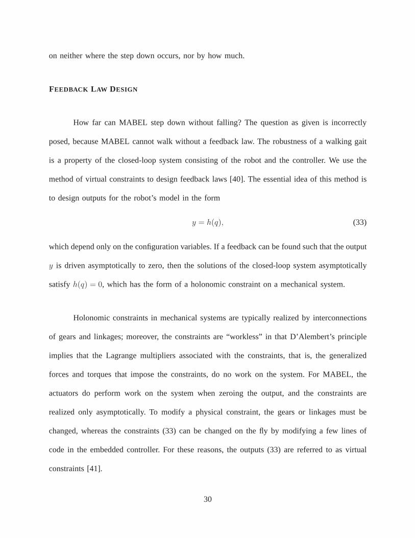
FEEDBACK L AW DESIGN

How far can MABEL step down without falling? The question as given is incorrectly

posed, because MABEL cannot walk without a feedback law. Therobustness of a walking gait

is a property of the closed-loop system consisting of the robot and the controller. We use the

method of virtual constraints to design feedback laws [40].The essential idea of this method is

to design outputs for the robot’s model in the form

y = h(q), (33)

which depend only on the configuration variables. If a feedback can be found such that the output

y is driven asymptotically to zero, then the solutions of the closed-loop system asymptotically

satisfyh(q) = 0, which has the form of a holonomic constraint on a mechanicalsystem.

Holonomic constraints in mechanical systems are typicallyrealized by interconnections

of gears and linkages; moreover, the constraints are “workless” in that D’Alembert’s principle

implies that the Lagrange multipliers associated with the constraints, that is, the generalized

forces and torques that impose the constraints, do no work onthe system. For MABEL, the

actuators do perform work on the system when zeroing the output, and the constraints are

realized only asymptotically. To modify a physical constraint, the gears or linkages must be

changed, whereas the constraints (33) can be changed on the fly by modifying a few lines of

code in the embedded controller. For these reasons, the outputs (33) are referred to as virtual

constraints [41].

30

We use virtual constraints to synchronize the evolution of MABEL’s links throughout a

stride in order to synthesize a walking gait. One virtual constraint per actuator is specified in

the form “output equals controlled variables minus desiredevolution.” Specifically,

y = h0(q)− hd (s, α) , (34)

where the controlled variables are

h0(q) =

qmLSst

qLAsw

qmLSsw

qT

, (35)

and whereqmLSstis the leg-shape-motor position of the stance leg,qLAsw

and qmLSsw are the

leg angle and leg-shape-motor position of the swing leg, andqT is the torso angle. The desired

evolution of the controlled variables in (35) is specified bythe functionshdmLSst

, hdLAsw

, hdmLSsw

,

andhdT, respectively, and assembled as

hd (s, α) =

hdmLSst

(s, α)

hdLAsw

(s, α)

hdmLSsw

(s, α)

hdT (s, α)

, (36)

whereα is a vector of real numbers parameterizing the virtual constraints. For MABEL, we

chooses as

s(q) =θ(q)− θ+

θ− − θ+, (37)

whereθ is the absolute angle formed by the virtual compliant leg relative to the ground, that is,

θ(q) = π − qLAst− qT, (38)

31

andθ+ and θ− are the values ofθ (q) at the beginning and end of a step, respectively. How to

construct the functions inhd (s, α) from Bezier polynomials and how to choose the parameters

to create a periodic walking gait in the closed-loop system is explained in [40] and [9]. The key

idea is to selectα to minimize a cost function representing energy supplied bythe actuators,

normalized by step length, with the minimization subject toboundary conditions that specify a

periodic solution, actuator magnitude and power limitations, friction limits in the ground contact

model, swing-leg clearance, and desired walking speed.

In principle, the virtual constraints can be implemented onthe robot by any feedback

capable of drivingy to zero. In the experiments described below, we use the feedforward-plus-

PD-controller

uexp(q, q) = u∗ (s(q), α)−KP y −KDy, (39)

whereu∗ (s(q), α) is nominal torque along the periodic orbit determined from the parameter

optimization problem when designing the gait, andy is defined in (34). The asymptotic stability

of the periodic orbit under this feedback law is verified on the model with a Poincare map, as

explained in [40] and [9].

The above process results in the virtual constraints depicted in Figure 24a. These

constraints correspond to a nominal walking gait from [9], which is modified so that the end

of the swing leg can clear a 2 cm obstacle, allowing the robot to step onto a platform before

stepping off it. In addition, the torso angle is adjusted so that the average walking speed is

0.95 m/s.

FIRST STEP-DOWN TEST

32

For the step-down test, MABEL is put in motion, walking around the central tower on

an initially flat floor. At the end of each lap, MABEL walks up a stair-stepped ramp, takes at

least one step on a flat platform, and then steps off the platform. The height of the platform

is increased each lap until the robot falls. Figure 25 illustrates how the ramp and platform are

constructed from a combination of 0.5 inch and 1.0 inch (2.54cm) thick sheets of plywood.

Using the control law (39) and the virtual constraints of Figure 24(a), MABEL succeeds

in stepping off heights of 0.5 inch, 1.0 inch, 1.5 inch, and 2.0 inch, before falling when the

platform height is increased to 2.5 inch (6.35 cm). A video ofthe experiment is available at

[42].

The fall is rather spectacular. MABEL steps off the platformonto its left leg, with no

apparent difficulty, but on the next step, when the right leg impacts the ground, the shin separates

into two pieces, causing the fall. In the video, the shin appears to suffer a devastating break, but in

reality, it is quite benign. To protect the ball bearings in the knees and hips from damage during

experiments such as this one, the shin contains a “mechanical fuse,” as shown in Figure 26.

The mechanical fuse joins the two pieces of the shin by plastic pins, which give way under a

sufficiently high impact. It takes about an hour to reassemble the shin.

Because the robot is not equipped with force sensors, it is not immediately obvious

whether the mechanical fuse is activated because the plastic pins are worn, or because the

impact forces are exceptionally large. Using the impact model of [43], however, which is based

on the change in generalized momentum when two objects collide, the contact intensityIF at the

leg end can be estimated from the experimental data.IF has units of N-s and represents, roughly

33

speaking, the integral of the contact force over the duration of the contact event. Table IX and

Figure 27 show the estimated contact intensity when walkingon flat ground and when stepping

off several raised platforms. The data indicate that, upon stepping off the 2.5 inch platform, the

contact event of the second step is more than four times as intense as when walking on flat

ground.

The step off the platform is expected to result in a more intense impact than the second

step. Further analysis of the data reveals what is happening. Figure 28 shows how the disturbance

at step-down causes the torso to pitch forward. The feedbacksystem overreacts when correcting

the torso angle, causing a second, rapid, forward-pitchingmotion of the torso. Because the angle

of the swing leg is controlled relative to the torso, the swing leg rotates forward rapidly as well

and impacts the ground with sufficient force to activate the fuse in the shin. Simulation of the

model developed in this article confirms this sequence of events, with the exception that the

model cannot predict that the shin actually breaks.

SECOND STEP-DOWN TEST

When MABEL steps off a platform, the height of the platform can be immediately

computed at impact from the lengths of the legs and the anglesof the joints. This information

can be used in the ensuing step to attenuate disturbances. Using the identified model, a new

set of virtual constraints is computed that reduces the impact intensity of the second step by

approximately 40%. These constraints are depicted in Figure 24(b).

The controller is modified to include a switch, as in [44]. Theoriginal virtual constraints

34

of Figure 24(a) are used in (34) and (39) until a step-down exceeding 2 cm is detected. The

detection of the step-down height takes place when the leg contacts the ground. For the ensuing

step, the virtual constraints of Figure 24(b) are substituted into (34), whereas, on the next step,

the original virtual constraints are reapplied.

With this modification to the control law, the step-down experiment is repeated. MABEL

steps down without falling from heights of 2.5 inch, 3.0 inch, and 3.5 inch (8.89 cm), at which

point the experiment is terminated, without the robot falling. Figure 29 shows the estimated

impact intensities for these tests.

CONCLUSIONS

Parameter identification of MABEL, a 5-link bipedal robot with a compliant transmission,

has been studied. For each side of the robot, the transmission is composed of three cable

differentials that connect two motors to the hip and knee joints in such a way that one motor

controls the angle of the virtual leg consisting of the line connecting the hip to the toe, while

the length of the virtual leg is controlled by a second motor connected in series with a spring.

The springs serve both to isolate the rotor inertia of the leg-shape motors from the impact forces

at leg touchdown and to subsequently store energy when the support leg must decelerate the

downward motion of the robot’s center of mass.

The robot is equipped with 14 encoders to measure motor, pulley, and joint angles,

as well as contact switches at the ends of the legs to detect impact with the ground. Neither

force sensors, torque sensors, nor accelerometers are available. To circumvent these limitations,

the identification procedure took advantage of the modular nature of the robot. By selectively

35

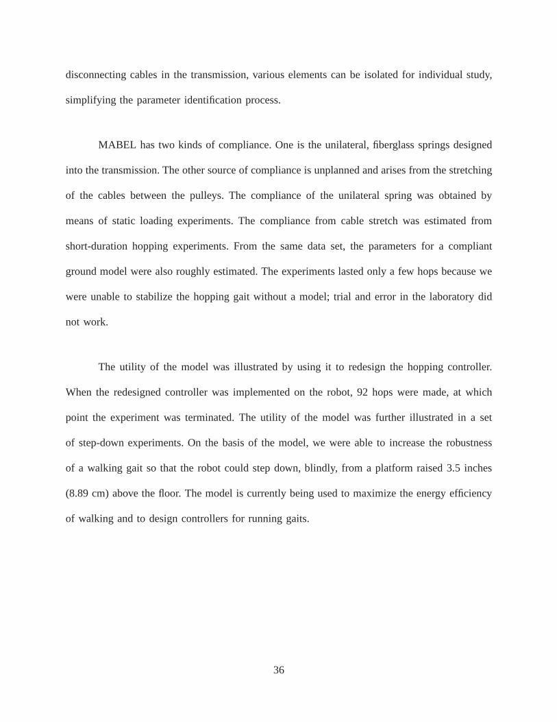
disconnecting cables in the transmission, various elements can be isolated for individual study,

simplifying the parameter identification process.

MABEL has two kinds of compliance. One is the unilateral, fiberglass springs designed

into the transmission. The other source of compliance is unplanned and arises from the stretching

of the cables between the pulleys. The compliance of the unilateral spring was obtained by

means of static loading experiments. The compliance from cable stretch was estimated from

short-duration hopping experiments. From the same data set, the parameters for a compliant

ground model were also roughly estimated. The experiments lasted only a few hops because we

were unable to stabilize the hopping gait without a model; trial and error in the laboratory did

not work.

The utility of the model was illustrated by using it to redesign the hopping controller.

When the redesigned controller was implemented on the robot, 92 hops were made, at which

point the experiment was terminated. The utility of the model was further illustrated in a set

of step-down experiments. On the basis of the model, we were able to increase the robustness

of a walking gait so that the robot could step down, blindly, from a platform raised 3.5 inches

(8.89 cm) above the floor. The model is currently being used tomaximize the energy efficiency

of walking and to design controllers for running gaits.

36

ACKNOWLEDGEMENTS

This work is supported by NSF grant ECS-909300. The authors thank J. Koncsol for

his selfless dedication to our project. His time in the laboratory, on his way to work or on

Saturday mornings, where he shared his extensive experience in electronic circuit design and

testing, was instrumental to our experiments. G. Buche is gratefully acknowledged for his many

contributions, especially the design of the power supply and safety systems. His prior experience

with Rabbit was invaluable in the initial setup of the MABEL testbed.

37

REFERENCES

[1] S. Collins, A. Ruina, R. Tedrake, and M. Wisse, “Efficientbipedal robots based on passive-

dynamic walkers,”Science, vol. 307, pp. 1082–1085, 2005.

[2] J. K. Hodgins, “Biped gait transitions,” inProc. of the IEEE Int. Conf. on Robotics and

Automation, Sacramento, CA, USA, April 1991, pp. 2092–2097.

[3] J. K. Hodgins and M. H. Raibert, “Adjusting step length for rough terrain locomotion,”IEEE

Trans. on Robotics and Automation, vol. 7, no. 3, pp. 289–298, June 1991.

[4] M. H. Raibert,Legged Robots That Balance. Cambridge, MA, USA: The MIT Press, 1986.

[5] C. Chevallereau, G. Abba, Y. Aoustin, F. Plestan, E. Westervelt, C. Canudas-De-Wit,

and J. Grizzle, “RABBIT: a testbed for advanced control theory,” IEEE Control Systems

Magazine, vol. 23, no. 5, pp. 57–79, Oct. 2003.

[6] E. R. Westervelt, G. Buche, and J. W. Grizzle, “Experimental validation of a framework for

the design of controllers that induce stable walking in planar bipeds,”The Int. J. of Robotics

Research, vol. 24, no. 6, pp. 559–582, June 2004.

[7] B. Morris, E. Westervelt, C. Chevallereau, G. Buche, andJ. Grizzle, “Achieving bipedal run-

ning with RABBIT: Six steps toward infinity,” inFast Motions Symposium on Biomechanics

and Robotics, K. Mombaur and M. Dheil, Eds. Heidelberg, Germany: Springer-Verlag,

2006, pp. 277–297.

[8] J. W. Hurst, J. E. Chestnutt, and A. A. Rizzi, “The actuator with mechanically adjustable

series compliance,”IEEE Trans. on Robotics, vol. 26, no. 4, pp. 597–606, 2010.

[9] K. Sreenath, H.-W. Park, I. Poulakakis, and J. W. Grizzle, “A compliant hybrid zero dynamics

controller for stable, efficient and fast bipedal walking onMABEL,” The Int. J. of Robotics

38

Research, published online, Sept. 21, 2010.

[10] W. Khalil and E. Dombre,Modeling, Identification and Control of Robots. Bristol, PA,

USA: Taylor & Francis, Inc., 2002.

[11] J. Swevers, W. Verdonck, and J. D. Schutter, “Dynamic model identification for industrial

robots,” IEEE Control Systems Magazine, vol. 27, no. 5, pp. 58–71, Oct. 2007.

[12] C. G. Atkeson, C. H. An, and J. M. Hollerbach, “Estimation of inertial parameters of

manipulator loads and links,”The Int. J. of Robotics Research, vol. 5, no. 3, pp. 101–119,

1986.

[13] M. Gautier and W. Khalil, “On the identification of the inertial parameters of robots,”

in Proc. of the IEEE Conf. on Decision and Control, Tampa, FL, USA, Dec. 1988, pp.

2264–2269.

[14] J. Hurst, J. Chestnutt, and A. Rizzi, “Design and philosophy of the bimasc, a highly dynamic

biped,” inProc. of the IEEE Int. Conf. on Robotics and Automation, Roma, Italy, April 2007,

pp. 1863–1868.

[15] J. Grizzle, J. Hurst, B. Morris, H.-W. Park, and K. Sreenath, “MABEL, a new robotic

bipedal walker and runner,” inProc. of the American Control Conf., St. Louis, MO, USA,

June 2009, pp. 2030–2036.

[16] J. W. Hurst, “The role and implementation of compliancein legged locomotion,” Ph.D.

dissertation, Robotics Institute, Carnegie Mellon University, Pittsburgh, PA, August 2008.

[Online]. Available at http://www.ri.cmu.edu/publication view.html?pubid=6179.

[17] M. A. Daley and A. A. Biewener, “Running over rough terrain reveals limb control for

intrinsic stability,” Proc. of the National Academy of Sciences, vol. 103, no. 42, pp. 15,681–

15,686, 2006.

39

[18] M. A. Daley, J. R. Usherwood, G. Felix, and A. A. Biewener, “Running over rough

terrain: guinea fowl maintain dynamic stability despite a large unexpected change in substrate

height,” J. of Experimental Biology, vol. 209, no. 1, pp. 171–187, 2006.

[19] J. Hodgins and M. Raibert, “Adjusting step length for rough terrain locomotion,”IEEE

Trans. on Robotics and Automation, vol. 7, no. 3, pp. 289–298, June 1991.

[20] K. Hashimoto, Y. Sugahara, H. Sunazuka, C. Tanaka, A. Ohta, M. Kawase, H. Lim,

and A. Takanishi, “Biped landing pattern modification method with nonlinear compliance

control,” in Proc. of the IEEE Int. Conf. on Robotics and Automation, Orlando, FL, USA,

May 2006, pp. 1213–1218.

[21] M. Ogino, H. Toyama, and M. Asada, “Stabilizing biped walking on rough terrain based on

the compliance control,” inProc. of IEEE/RSJ Int. Conf. on Intelligent Robots and Systems,

San Diego, CA, USA, Nov. 2007, pp. 4047–4052.

[22] U. Saranli, M. Buehler, and D. E. Koditschek, “RHex: A simple and highly mobile hexapod

robot,” The Int. J. of Robotics Research, vol. 20, pp. 616–631, 2001.

[23] T. Takuma, S. Hayashi, and K. Hosoda, “3D bipedal robot with tunable leg compliance

mechanism for multi-modal locomotion,” inProc. of IEEE/RSJ Int. Conf. on Intelligent

Robots and Systems, Nice, France, Sept. 2008, pp. 1097–1102.

[24] A. Dabroom and H. Khalil, “Numerical differentiation using high-gain observers,” inProc.

of the IEEE Conf. on Decision and Control, San Diego, CA, USA, 1997, pp. 4790–4795.

[25] M. Mboup, C. Join, and M. Fliess, “A revised look at numerical differentiation with an

application to nonlinear feedback control,” inProc. of Mediterranean Conf. on Control &

Automation, Ajaccio, France, 2008, pp. 1–6.

[26] J. Swevers, W. Verdonck, and J. De Schutter, “Dynamic model identification for industrial

40

robots,” IEEE Control Systems Magazine, vol. 27, no. 5, pp. 58–71, 2007.

[27] S. Diop, J. W. Grizzle, P. E. Moraal, and A. Stefanopoulou, “Interpolation and numerical

differentiation for observer design,” inProc. of the American Control Conf., Baltimore, MD,

USA, 1994, pp. 1329–1333.

[28] U. Saranli, M. Buehler, and D. E. Koditschek, “RHex: A simple and highly mobile hexapod

robot,” The Int. J. of Robotics Research, vol. 20, no. 1, pp. 616–631, July 2001.

[29] uBLAS - Basic Linear Algebra Subprograms library. [Online]. Available at http:

//www.boost.org

[30] D. Marhefka and D. Orin, “Simulation of contact using a nonlinear damping model,” in

Proc. of the IEEE Int. Conf. on Robotics and Automation, vol. 2, Minneapolis, MN, USA,

April 1996, pp. 1662–1668.

[31] C. Canudas de Wit, H. Olsson, K. Astrom, and P. Lischinsky, “A new model for control

of systems with friction,”IEEE Trans. on Automatic Control, vol. 40, no. 3, pp. 419–425,

Mar. 1995.

[32] F. Plestan, J. Grizzle, E. Westervelt, and G. Abba, “Stable walking of a 7-DOF biped robot,”

IEEE Trans. on Robotics and Automation, vol. 19, no. 4, pp. 653–668, Aug. 2003.

[33] J. Swevers, C. Ganseman, D. Tukel, J. de Schutter, and H.Van Brussel, “Optimal robot

excitation and identification,”IEEE Trans. on Robotics and Automation, vol. 13, no. 5, pp.

730–740, Oct. 1997.

[34] F. Pfeiffer and J. Holzl, “Parameter identification forindustrial robots,” inProc. of the IEEE

Int. Conf. on Robotics and Automation, vol. 2, Nagoya, Japan, May 1995, pp. 1468–1476.

[35] P. Vandanjon, M. Gautier, and P. Desbats, “Identification of robots inertial parameters by

means of spectrum analysis,” inProc. of the IEEE Int. Conf. on Robotics and Automation,

41

vol. 3, Nagoya, Japan, May 1995, pp. 3033–3038.

[36] K. Kozlowski, Modelling and Identification in Robotics. Secaucus, NJ, USA: Springer-

Verlag, 1998.

[37] M. Wisse, A. L. Schwab, R. Q. van der Linde, and F. C. T. vander Helm, “How to

keep from falling forward: Elementary swing leg action for passive dynamic walkers,”IEEE

Trans. on Robotics, vol. 21, no. 3, pp. 393–401, June 2005.

[38] C. Sabourin, O. Bruneau, and G. Buche, “Control strategy for the robust dynamic walk of

a biped robot,”The Int. J. of Robotics Research, vol. 25, no. 9, pp. 843–860, Sept. 2006.

[39] M. Wisse and R. Q. van der Linde,Delft Pneumatic Bipeds. Springer, 2007.

[40] E. R. Westervelt, J. W. Grizzle, C. Chevallereau, J. H. Choi, and B. Morris,Feedback

Control of Dynamic Bipedal Robot Locomotion. Taylor & Francis/CRC Press, 2007.

[41] C. C. de Wit, “On the concept of virtual constraints as a tool for walking robot control

and balancing,”Annual Reviews in Control, vol. 28, no. 2, pp. 157–166, 2004.

[42] J. W. Grizzle. Dynamic leg locomotion. Youtube Channel. [Online]. Available at

http://www.youtube.com/DynamicLegLocomotion

[43] Y. Hurmuzlu and D. B. Marghitu, “Rigid Body Collisions of Planar Kinematic Chains With

Multiple Contact Points,”The Int. J. of Robotics Research, vol. 13, no. 1, pp. 82–92, 1994.

[44] T. Yang, E. Westervelt, and A. Serrani, “A framework forthe control of stable aperiodic

walking in underactuated planar bipeds,” inProc. of the IEEE Int. Conf. on Robotics and

Automation, Roma, Italy, April 2007, pp. 4661–4666.

42

(a) (b)

Figure 1: MABEL, a planar bipedal robot for walking and running. (a) The shin and thigh are

each 50 cm long, making the robot 1 m tall at the hip. The overall mass is 60 kg, excluding

the boom. The boom provides side-to-side stability becausethe hips are revolute joints allowing

only forward and backward motion of the legs. The safety cable prevents the knees and torso

from hitting the lab floor when the robot falls. (b) The robot incorporates springs for shock

absorption and energy storage. Differentials housed in therobot’s torso create a virtual prismatic

leg with compliance.

43

Figure 2: Approximate planar motion. The boom constrains MABEL’s motion to the surface

of a sphere centered at the attachment point of the boom to thecentral tower. The boom is

approximately 2.25 m long. The central tower is supported ona slip ring through which power

and digital communication lines, such as E-stop and ethernet, are passed.

44

rx,T

ry,T

rx,Th

ry,Csh

rx,Csh

rx,Csp

ry,Csp

rx,Sh

ry,Sh

ry,Th

mCsp

,JCsp

mT ,J

T

mCsh

,JCsh

mTh

,JTh

mSh

,JSh

(a)

Shin

0.5

mLS Step-down

mLS Motor

-1

AS

pri

ng

- +

mLA Step-down

mLA Motor

0.5

+ +

qmLA

qmLS

qBsp

qLS

qLA

qTh

qSh

Thigh

BS

pri

ng

CSpring

DSpring

CShin

AS

hin

BS

hin

DShin

AT

hig

h

BT

hig

h

DThigh

CThigh

(b)

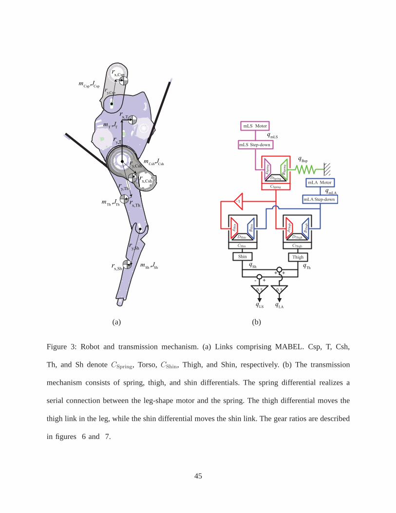
Figure 3: Robot and transmission mechanism. (a) Links comprising MABEL. Csp, T, Csh,

Th, and Sh denoteCSpring, Torso,CShin, Thigh, and Shin, respectively. (b) The transmission

mechanism consists of spring, thigh, and shin differentials. The spring differential realizes a

serial connection between the leg-shape motor and the spring. The thigh differential moves the

thigh link in the leg, while the shin differential moves the shin link. The gear ratios are described

in figures 6 and 7.

45

(a) (b)

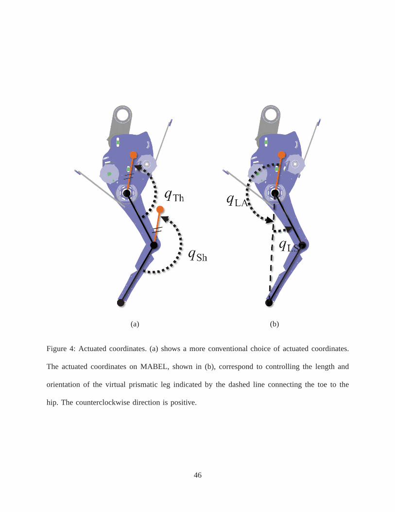
Figure 4: Actuated coordinates. (a) shows a more conventional choice of actuated coordinates.

The actuated coordinates on MABEL, shown in (b), correspondto controlling the length and

orientation of the virtual prismatic leg indicated by the dashed line connecting the toe to the

hip. The counterclockwise direction is positive.

46

(a) (b)

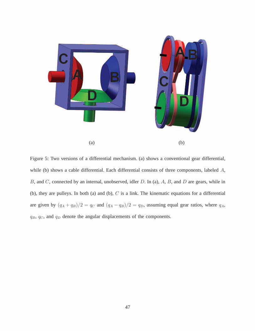
Figure 5: Two versions of a differential mechanism. (a) shows a conventional gear differential,

while (b) shows a cable differential. Each differential consists of three components, labeledA,

B, andC, connected by an internal, unobserved, idlerD. In (a),A, B, andD are gears, while in

(b), they are pulleys. In both (a) and (b),C is a link. The kinematic equations for a differential

are given by(qA + qB)/2 = qC and (qA − qB)/2 = qD, assuming equal gear ratios, whereqA,

qB, qC , andqD denote the angular displacements of the components.

47

(a) qLA pulley system

AS

hin

AT

hig

h

BT

high

BS

hin

Shin

0.5qLS

- +

mLA step-down

mLA Motor

CShin

0.5+ +

qLA

11.77

-

11.7711.77

23.53

23.5323.53

23.53

DShin DThigh

-

--

-

--

-

CThigh

ω

ω

ωω

ω

ω

ω

ω

Thigh23.53

-ω

(b) qLA Transmission

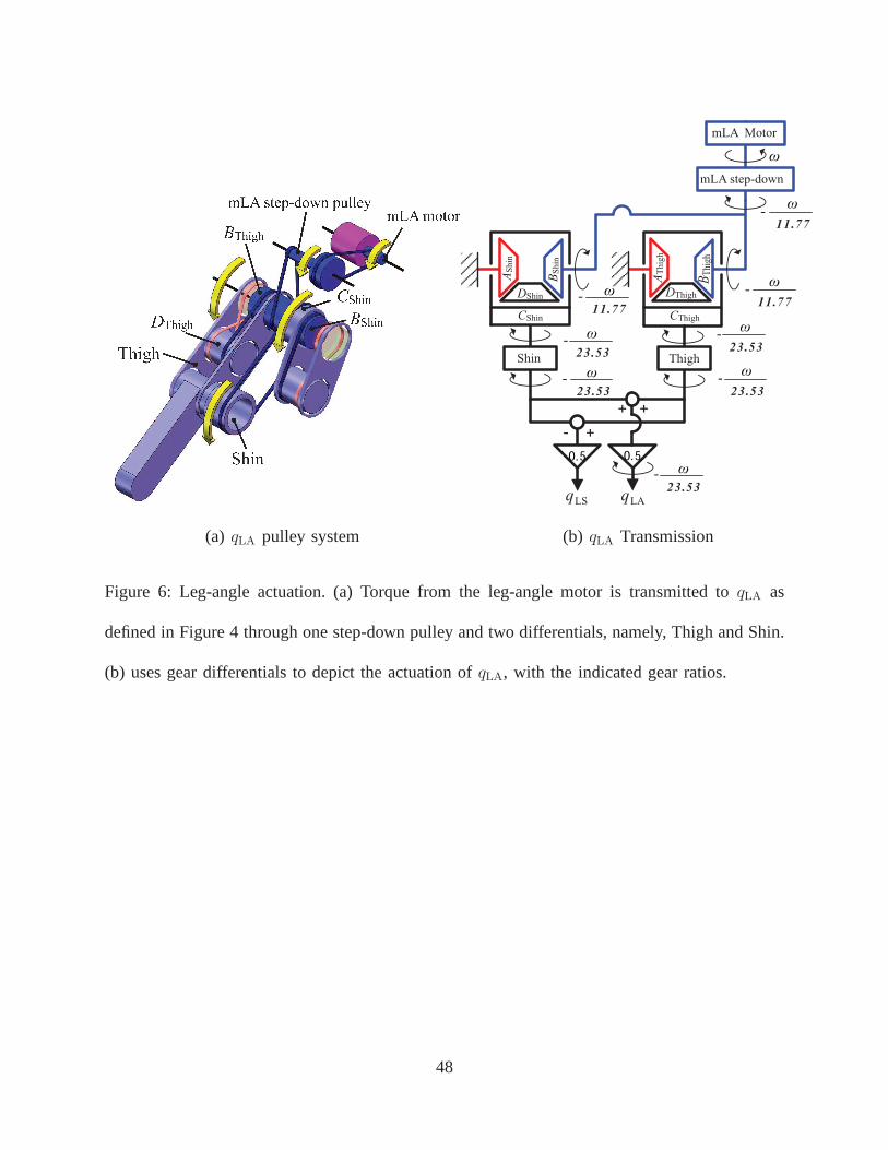
Figure 6: Leg-angle actuation. (a) Torque from the leg-angle motor is transmitted toqLA as

defined in Figure 4 through one step-down pulley and two differentials, namely, Thigh and Shin.

(b) uses gear differentials to depict the actuation ofqLA, with the indicated gear ratios.

48

mLS Motor

mLS step-down

pulley

DSpring

Thigh

CSpring

CSpring

AShin

CShinDShin

DThigh

Shin

AThigh

ASpring

(a) qLS pulley system

AS

hin

AT

hig

h

BT

hig

h

BS

hin

Shin

0.5qLS

mLS step-down

mLS Motor

-1

AS

pri

ng

BS

pri

ng

- +

CShin

CSpring

CThigh

0.5

+ +

qLA

-31.42

-15.71 15.71

15.71

9.647

31.42

-31.42

31.42

DSpring

DThighDShin

ω

ω

ω

ω ω

ω

ω ω

ω

Thigh31.42

ω

(b) qLS transmission

Figure 7: Leg-shape actuation. (a) Torque from the leg-shape motor is transmitted toqLS as

defined in Figure 4 through one step-down pulley and three differentials, namely, Spring, Thigh,

and Shin. (b) uses gear differentials to depict the actuation of qLS, with the indicated gear ratios.

49

Differentials

Shin

Link

Amplifier

Command

Current

Output MeasurementInput Measurement

Motor

Encoder

Amplifier

Command

Input Measurement

Motor

Encoder

Output Measurement

Thigh

Link

Torso

Fixed

Knee

Encoder

MLA Step- down

Encoder

DThigh

Encoder

BSpring

Encoder

Thigh

Encoder

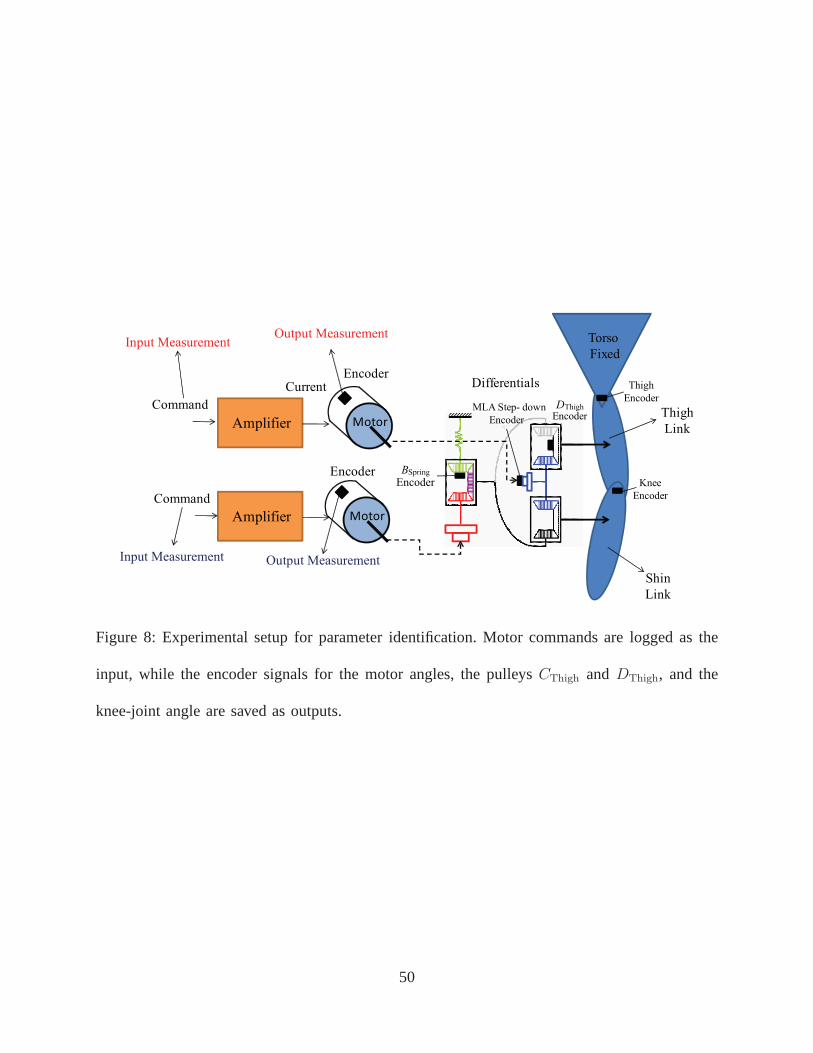
Figure 8: Experimental setup for parameter identification.Motor commands are logged as the

input, while the encoder signals for the motor angles, the pulleys CThigh andDThigh, and the

knee-joint angle are saved as outputs.

50

mLA

Step-down

BThigh

Experiment-1

Experiment-3

Experiment-2

Step-down

BShin

mLA

mLA BThigh

BShinDThigh

DShin

(a)

mLS

Step-down

ASpring

Experiment-1

Experiment-2

Experiment-3

Step-down

mLS

mLS ASpring DSpring

(b)

Figure 9: Pulley choices for identifying the transmission parameters. (a)qLA path and (b)qLS

path. The various pulley combinations are formed by selectively disconnecting cables in the

transmission. If the inertias of the pulleys are known, thentwo pulley combinations are sufficient

to identify the inertia of the motor rotor and the torque constant. By adding a third pulley

combination, the pulley inertias provided by the CAD program can be validated.

51

Sinusoidally

Varying Frequency

and Magnitude

Motor PulleyEncoder Signal

Identify Transfer Function

Motor Correction Factor Pulleys, Cable, and Rotor

1αtorque

1Jis+µi

1Jexp,is+µexp,i

=1

αtorque(Jis+µi)

K1+Tps

=1

Jexp,is+µexp,i

Jexp,i =Tp

K, µexp,i =

1K

Figure 10: Transfer function from the the amplifier command input to the motor encoder signal

output. The parameterαtorque is the correction factor for the motor torque constant supplied by

the manufacturer. The measured transfer function is1/ [αtorque(Jis + µi)]. The Matlab System

Identification Toolbox is used to estimate the first-order transfer function from the measured

data.

52

0 10 20 30 40 50 60 70 80

Outp

ut

(deg

)

0 10 20 30 40 50 60 70 80

5

0

0.5

1

1.5

time (s)

Input

(N-m

)

1 Hz 1.1 Hz ... ... ...... ... ...1.2 Hz 2.0 Hz

Figure 11: Illustrative input and output for system identification. The input is a modified chirp

signal, that is, a sinusoid with time-varying frequency andmagnitude. Each frequency is held

constant until the system reaches steady state.

53

Simulation

Model

MABEL

, torque

Input Sequence

Transmission

IdentificationCAD Program

Simulated Output

b,

Optimization

rotor αα θ μ

Measured Output

Figure 12: Simulation and validation procedures for leg identification. Identical input sequences

are applied to the simulation model and MABEL. The simulation model uses the motor

parameters estimated from the transmission identificationalong with the mass-inertia parameters

calculated from the CAD program, while torque bias and friction coefficients are free variables

used to fit the simulation data to the experimental data. In the validation step, a new input

sequence is used and the motor bias is re-estimated, while all remaining parameters are held

constant.

54

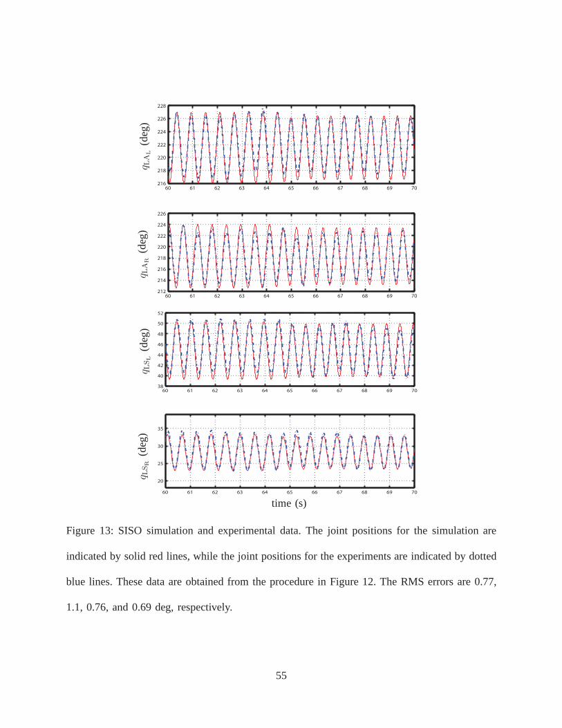
60 61 62 63 64 65 66 67 68 69 70216

218

220

222

224

226

228

60 61 62 63 64 65 66 67 68 69 70212

214

216

218

220

222

224

226

q LA

L(d

eg)

q LA

R(d

eg)

60 61 62 63 64 65 66 67 68 69 7038

40

42

44

46

48

50

52

60 61 62 63 64 65 66 67 68 69 70

20

25

30

35

q LSL

(deg

)q L

SR

(deg

)

time (s)

Figure 13: SISO simulation and experimental data. The jointpositions for the simulation are

indicated by solid red lines, while the joint positions for the experiments are indicated by dotted

blue lines. These data are obtained from the procedure in Figure 12. The RMS errors are 0.77,

1.1, 0.76, and 0.69 deg, respectively.

55

30 35 40 45170

172

174

176

178

180

182

30 35 40 455

10

15

20

25

30

q LA

L(d

eg)

q LSL

(deg

)

30 35 40 45160

165

170

175

180

30 35 40 4510

15

20

25

30

q LA

R(d

eg)

q LSR

(deg

)

time (s)

Figure 14: MIMO simulation and experimental data. The jointpositions for the simulation are

indicated by solid red lines, while the joint positions for the experiments are indicated by dotted

blue lines. These data are obtained from the procedure in Figure 12. The RMS errors are 1.0,

1.42, 1.14, and 0.72 deg, respectively.

56

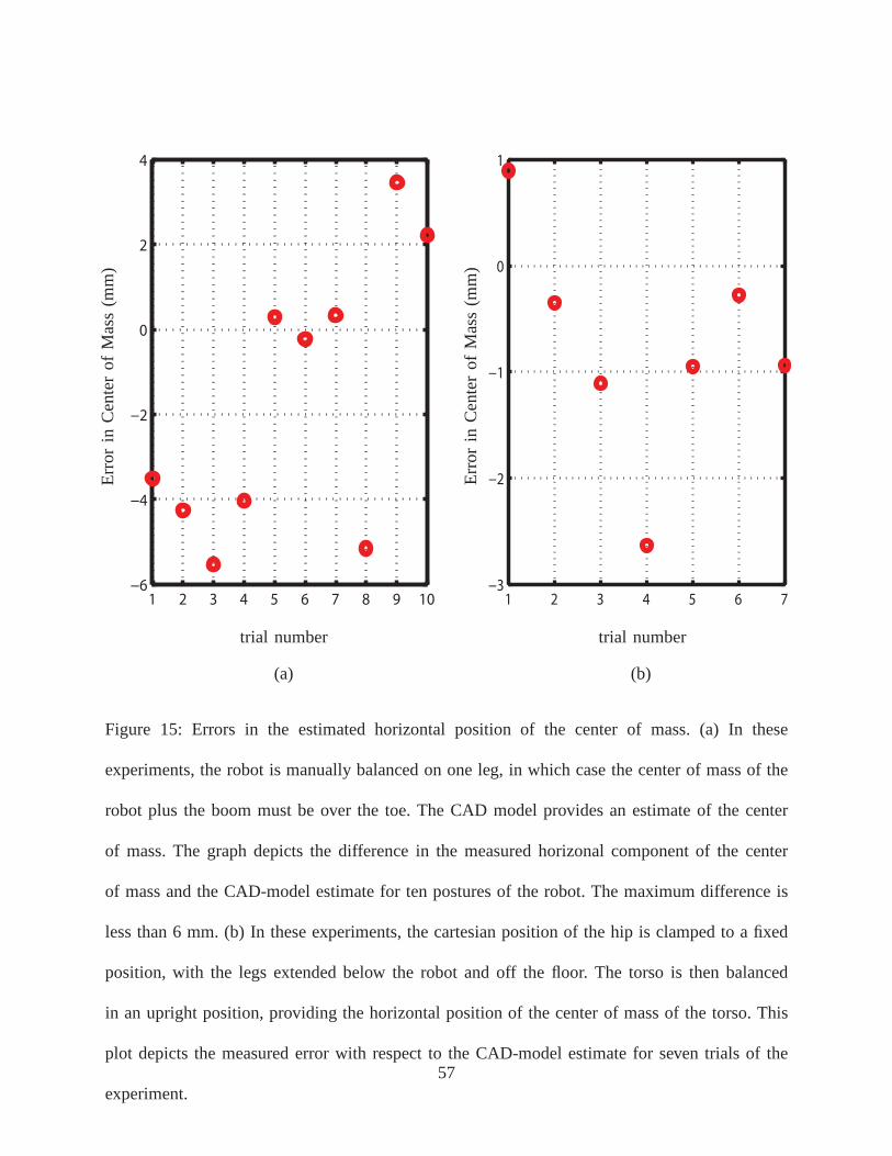
1 2 3 4 5 6 7 8 9 10

0

2

4

trial number

Err

or

inC

ente

ro

fM

ass

(mm

)

(a)

1 2 3 4 5 6 7

0

1

trial number

Err

or

inC

ente

ro

fM

ass

(mm

)

(b)

Figure 15: Errors in the estimated horizontal position of the center of mass. (a) In these

experiments, the robot is manually balanced on one leg, in which case the center of mass of the

robot plus the boom must be over the toe. The CAD model provides an estimate of the center

of mass. The graph depicts the difference in the measured horizonal component of the center

of mass and the CAD-model estimate for ten postures of the robot. The maximum difference is

less than 6 mm. (b) In these experiments, the cartesian position of the hip is clamped to a fixed

position, with the legs extended below the robot and off the floor. The torso is then balanced

in an upright position, providing the horizontal position of the center of mass of the torso. This

plot depicts the measured error with respect to the CAD-model estimate for seven trials of the

experiment.57

gravity

kg

yyyy

τAsp

τgravity

τBsp

Figure 16: Experimental setup for measuring spring stiffness and pre-load. Pulley Asp is locked

in place by commanding the leg-shape motor to a fixed orientation. Consequently, the torque

due to gravityτgravity must be balanced by the torque from the springτBsp. The resulting spring

deflectionqBsp is measured and recorded.

58

0.1 0.2 0.3 0.4 0.5 0.620

30

40

50

60

70

qBspL (rad)

τ Bsp

L(N

-m)

(a) Left Spring

0.1 0.2 0.3 0.4 0.5 0.620

30

40

50

60

70

qBspR (rad)

τ Bsp

R(N

-m)

(b) Right Spring

Figure 17: Measurements of torqueτBsp versus displacementqBsp obtained from the experimental

setup of Figure 16. The data in (a) are fit byτBspL = 115.1qBspL + 2.214. The fit shows that,

on the left side of the robot, the spring stiffness is115.1 N-m per rad and the pre-load offset is

2.214 N-m. On the right side of the robot, the data in (b) are fitby τBspR = 111.7qBspR +5.377,

showing that the spring stiffness is111.7 N-m per rad and the pre-load offset is 5.377 N-m. The

estimated values of spring stiffness and pre-load are consistent on the left and right sides of the

robot.

59

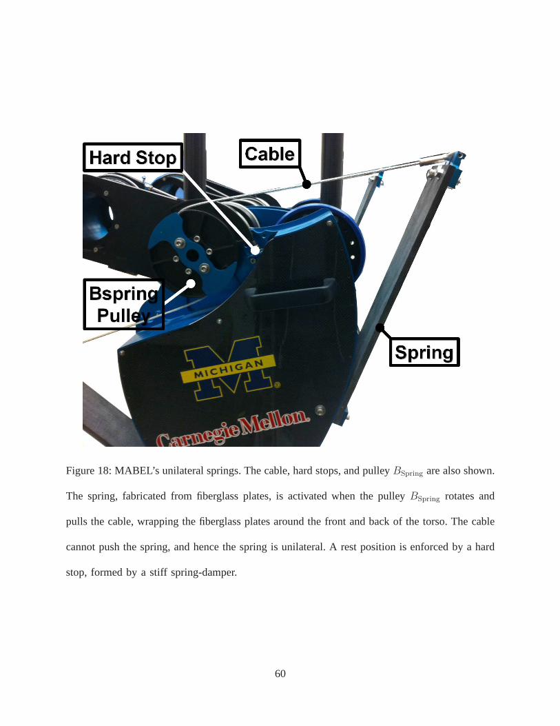
Figure 18: MABEL’s unilateral springs. The cable, hard stops, and pulleyBSpring are also shown.

The spring, fabricated from fiberglass plates, is activatedwhen the pulleyBSpring rotates and

pulls the cable, wrapping the fiberglass plates around the front and back of the torso. The cable

cannot push the spring, and hence the spring is unilateral. Arest position is enforced by a hard

stop, formed by a stiff spring-damper.

60

21 21.2 21.4 21.6 21.8 22 22.2140

145

150

155

160

21 21.2 21.4 21.6 21.8 22 22.2180

185

190

195

21 21.2 21.4 21.6 21.8 22 22.20

10

20

30

21 21.2 21.4 21.6 21.8 22 22.20

10

20

30

40

qLA

L(d

eg)

qLA

R(d

eg)

qLSL

(deg

)qLSR

(deg

)

time (s)

Figure 19: Validation data from the second hopping experiment. The joint positions for the

simulation are indicated by solid red lines, while the jointpositions for the experiment are

indicated by dotted blue lines. Though the hopping controller is not based on trajectory tracking,

the variables shown are indirectly regulated by the feedback controller, which may be responsible

for the close correspondence between the modeled and measured data.

61

21 21.2 21.4 21.6 21.8 22 22.2−10

0

10

20

30

21 21.2 21.4 21.6 21.8 22 22.2−20

0

20

40

60

qBsp

L(d

eg)

qBsp

R(d

eg)

21 21.2 21.4 21.6 21.8 22 22.2−5

0

5

10

15

21 21.2 21.4 21.6 21.8 22 22.2−5.2

−5

−4.8

−4.6

21 21.2 21.4 21.6 21.8 22 22.20.8

0.9

1

1.1

qT

(deg

)ph hip

(m)

pv hip

(m)

time (s)

Figure 20: Validation data from the second hopping experiment. The joint and hip positions

for the simulation are indicated by solid red lines, while the joint and hip positions for the

experiment are indicated by dotted blue lines. For these variables, the close correspondence

between the modeled and the measured data supports the model.

62

21 21.2 21.4 21.6 21.8 22 22.2−10

0

10

21 21.2 21.4 21.6 21.8 22 22.2−10

0

10

21 21.2 21.4 21.6 21.8 22 22.2−20

−10

0

10

21 21.2 21.4 21.6 21.8 22 22.2−40

−20

0

20

τ mLA

L(N

-m)

τ mLA

R(N

-m)

τ mLSL

(N-m

)τ m

LSR

(N-m

)

time (s)

Figure 21: Validation data from the second hopping experiment. The motor torques for the

simulation are indicated by solid red lines, while the motortorques for the experiment are

indicated by dotted blue lines. The ability to predict torque is an accepted measure of fit for

models of mechanical systems.

63

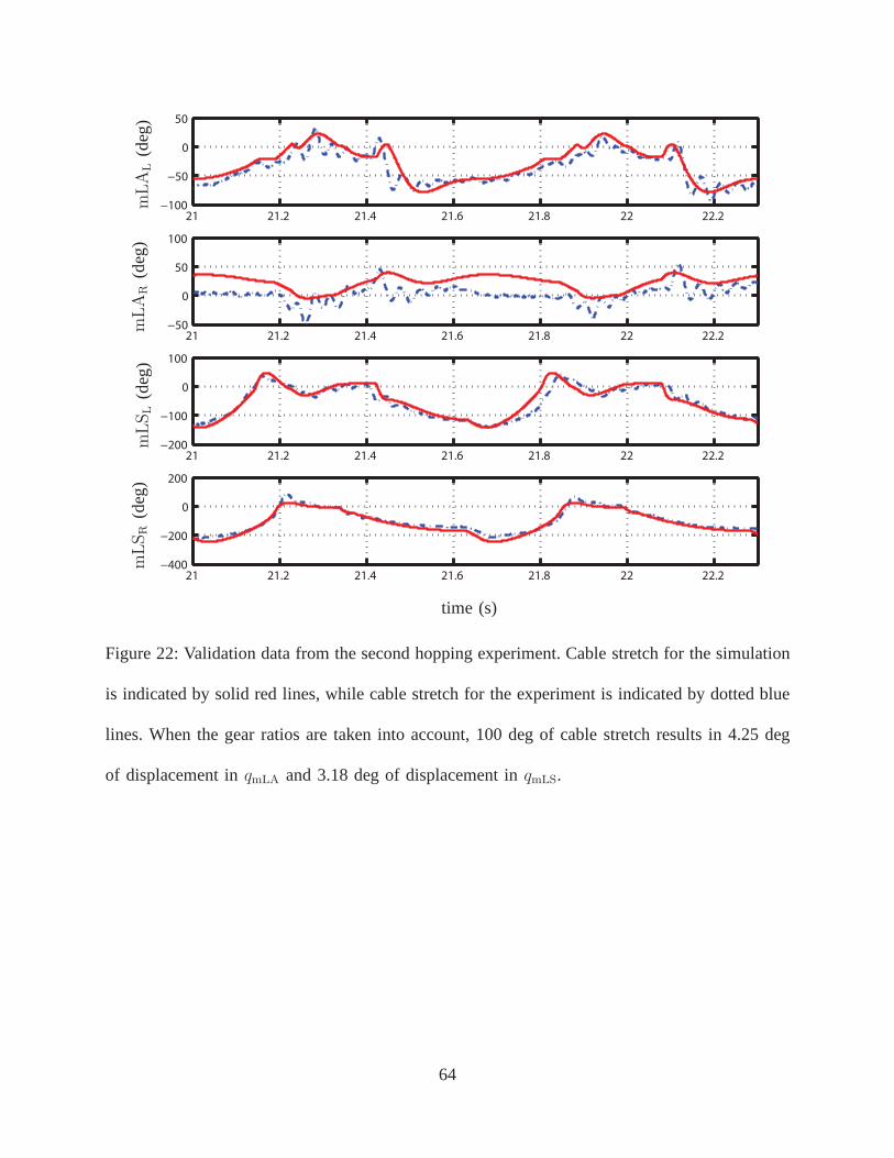
21 21.2 21.4 21.6 21.8 22 22.2−100

−50

0

50

21 21.2 21.4 21.6 21.8 22 22.2−50

0

50

100

21 21.2 21.4 21.6 21.8 22 22.2−200

−100

0

100

21 21.2 21.4 21.6 21.8 22 22.2−400

−200

0

200

mLA

L(d

eg)

mLA

R(d

eg)

mLSL

(deg

)mLSR

(deg

)

time (s)

Figure 22: Validation data from the second hopping experiment. Cable stretch for the simulation

is indicated by solid red lines, while cable stretch for the experiment is indicated by dotted blue

lines. When the gear ratios are taken into account, 100 deg ofcable stretch results in 4.25 deg

of displacement inqmLA and 3.18 deg of displacement inqmLS.

64

Figure 23: Stick figure illustration of a step-down experiment. The robot walks on a flat section

of flooring and then steps down to another flat section of flooring. The robot blindly walks off

the raised section of flooring; no information on where the step-down occurs, or the magnitude

of the step is provided to the robot. This figure is generated from experimental data of MABEL

stepping down from a height of 3.5 inch (8.89 cm).

65

170

180

190

200

210

qLA

sw(d

eg)

0

200

400

600

qmLS

sw(d

eg)

−6

−5

−4

−3

qTor

(deg

)

0 0.1 0.2 0.3 0.4 0.5 0.6 0.7 0.8 0.9 1450

500

550

qmLS

st(d

eg)

s

(a)

170

180

190

200

210

qLA

sw(d

eg)

0

200

400

600

qmLS

sw(d

eg)

−15

−10

−5

0

qTor

(deg

)

0 0.1 0.2 0.3 0.4 0.5 0.6 0.7 0.8 0.9 1510

520

530

540

qmLS

st(d

eg)

s

(b)

Figure 24: Virtual constraints used in the feedback controller. (a) shows the constraints used in

the first step-down experiment. (b) shows the additional virtual constraints used in the switching

controller of the second step-down experiment.

66

Figure 25: Plywood boards used to form a stair-stepped platform. By combining boards that are

1 inch (2.54 cm) and 0.5 inch (1.27 cm) thick, platforms of a desired height are assembled.

67

(a) (b)

Figure 26: Mechanical fuse in the shin. The shin of the robot is in (a), while (b) provides an

exploded view from the CAD drawings. The two parts of the shinare affixed with plastic pins.

The pins shear if the leg-ground impact generates a sufficiently large force, thus protecting other

parts of the robot, such as the knee and hip ball bearings, from damage.

68

0

5

10

15

20

25

30

35

40

45

50

1st step2nd step

flatground 1.0 inch 1.5 inch 2.0 inch 2.5 inch

Imp

act

Inte

nsi

ty(N

-s)

Figure 27: Impact intensity calculated from the first step-down experiment. Only the vertical

component is displayed. The green bar shows the average impact intensity when walking on flat

ground; the bars show± one standard deviation. The blue bar shows the impact intensity upon

step-down, while the red bar shows impact intensity for the ensuing step. The larger impact

intensity on the step following the 2.5 inch (6.35 cm) step-down leads to the fuse activating in

the shin.

69

0 0.2 0.4 0.6 0.8 1−20

−18

−16

−14

−12

−10

−8

−6

−4

−2

0

2

time (s)

Tors

oA

ng

le(d

eg)

experimentsimulation

Figure 28: Experimental and simulation data of the torso angle when stepping down from

the 2.5 inch platform. The forward direction is counterclockwise, and hence corresponds to

decreasing angles. The red and blue circles show when the swing leg impacts the ground.

The torso undergoes a large oscillation as a result of the disturbance at step-down. The same

behavior is observed in the model and the experiment, with the exception that, on the second

step at 0.943 s, the robot’s leg breaks, causing the torso to continue rotating forward.

70

0

5

10

15

20

25

30

35

40

45

50

2.5 inch 2.0 inch 2.5 inch 3.0 inch 3.5 inchfirsttest second test

experimentsimulation

Imp

act

Inte

nsi

ty(N

-s)

Figure 29: Impact intensities of the second step-down experiment. The solid bar is the vertical

component of the impact intensity of the second step, computed from the experimental data.

The hashed bar shows the values predicted by the simulation.

71

TABLE I: Notation for MABEL’s coordinates and torques. The subscriptsL andR denote the

left leg and right leg, respectively.

qLSL,Rleg-shape angle

qmLSL,Rmotor leg-shape angle

qLAL,Rleg-angle angle

qmLAL,Rmotor leg-angle angle

qBspL,Rpulley-BSpring angle

τmLSL,Rleg-shape motor torque

τmLAL,Rleg-angle motor torque

τBspL,Rpulley-BSpring torque

72

TABLE II: Parameters to be identified, wherei ∈ I, ℓ ∈ L, andt ∈ T . The subscriptsL andR

denote the left leg and right leg, respectively.

Differentials and Motors

Ki motor torque constant

Jrotor,i inertia of the rotor

Jt inertia of the transmission pulleys

µi friction coefficient

bi motor bias

Thigh and Shin (Leg)

mℓ mass of the linkℓ

Jℓ inertia of the linkℓ

mℓrx,ℓ center of mass in x-direction of the

link ℓ multiplied by mass of the linkℓ

mℓry,ℓ center of mass in y-direction of the

link ℓ multiplied by mass of the linkℓ

Compliance (Spring)

KBL,Rspring stiffness

KdBL,Rspring damping coefficient

KC,i cable stretch stiffness

KdC,i cable stretch damping coefficient

73

TABLE III: Moments of inertia of the pulleys in the transmission as obtained from the CAD

model.

PulleyMoment of inertia

(kg-m2)

JmLS 9.0144e-4

JmLA 4.4928e-4

JAth 1.6680e-3

JBth 2.2181e-3

JDth 1.0826e-3

JAsh 1.6974e-3

JBsh 2.2181e-3

JDsh 2.0542e-3

JAsp 2.3464e-3

JBsp 1.8686e-3

JDsp 1.9313e-3

JmLSsd 2.7117e-3

JmLAsd 1.0950e-3

74

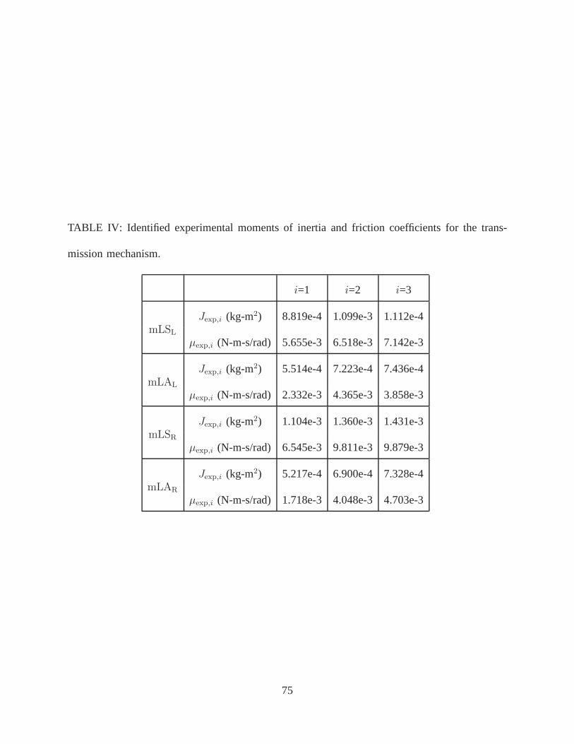
TABLE IV: Identified experimental moments of inertia and friction coefficients for the trans-

mission mechanism.

i=1 i=2 i=3

mLSL

Jexp,i (kg-m2) 8.819e-4 1.099e-3 1.112e-4

µexp,i (N-m-s/rad) 5.655e-3 6.518e-3 7.142e-3

mLAL

Jexp,i (kg-m2) 5.514e-4 7.223e-4 7.436e-4

µexp,i (N-m-s/rad) 2.332e-3 4.365e-3 3.858e-3

mLSR

Jexp,i (kg-m2) 1.104e-3 1.360e-3 1.431e-3

µexp,i (N-m-s/rad) 6.545e-3 9.811e-3 9.879e-3

mLAR

Jexp,i (kg-m2) 5.217e-4 6.900e-4 7.328e-4

µexp,i (N-m-s/rad) 1.718e-3 4.048e-3 4.703e-3

75

TABLE V: Motor parameters. The rotor inertiasJrotor,man and torque constantsKT,man are

provided by the manufacturer. The correction factorsαrotor and αtorque as well as the motor

biasesb are estimated from experimental data.

mLSL mLAL mLSR mLAR

Jrotor,man (kg-m2) 8.755e-4 4.880e-4 8.755e-4 4.880e-4

KT,man (N-m/A) 1.516 0.577 1.516 0.577

αrotor 0.934 0.741 0.930 0.763

αtorque 0.995 1.332 1.287 1.269

b (N-m) -0.1076 -0.04652 0.02995 -0.001672

76

TABLE VI: Mass, center of mass, and moment of inertia of the links obtained from the CAD

model. The center of mass coordinatesrx and ry are defined in Figure 3(a), while the moment

of inertia is defined about the joint that passes through the origin of the corresponding link in

Figure 3(a).

LinkMass Center of Mass Moment of inertia Length

(kg) [rx, ry] (m) (kg-m2) (m)

Spring (Csp) 1.8987 [0.0009406, 0.1181] 0.04377 -

Torso (T) 40.8953 [0.01229, 0.18337] 2.3727 -

Cshin (Csh) 1.6987 [0.0004345, 0.08684] 0.03223 -

Thigh (Th) 3.2818 [0.0003110, 0.1978] 0.1986 0.5

Shin (Sh) 1.5007 [0.0009671, 0.1570] 0.08813 0.5

Boom 7.2575 [0.0, 1.48494153] 20.4951 2.25

77

TABLE VII: Estimates of friction coefficientsµ and motor biasesb obtained by minimizing the

costs in (17) and (18), respectively.

i = mLSL i = mLAL i = mLSR i = mLAR

µi (N-m-s/rad) 9.844e-3 4.316e-3 9.027e-3 4.615e-3

bi (N-m) -8.417e-3 2.597e-2 -1.446e-2 -2.461e-3

78

TABLE VIII: Parameters estimated from the dynamic hopping experiment.

Spring Model

KdB (N-m-s/rad) 1.5 Kvd1 (N-m-s/rad) 1000

Kd1 (N-m/rad3) 100 Kvd2 (N-m/(rad/s)0.5) 50

Cable Stretch Model

i = mLSL i = mLAL i = mLSR i = mLAR

KC,i (N-m/rad) 2.9565 3.5000 2.9565 3.8094

KdC,i (N-m-s/rad) 0.0402 0.0889 0.0804 0.3556

Ground Model

λav (N/m1.5/(m/s)) 3.0e6 σh0 (N/m) 260.0

λbv (N/m1.5/(m/s)0.5) 4.5e6 σh1 (N-s/m) 2.25

n 1.5 αh0 (N) 1.71

k (N/m1.5) 4.38e7 αh2 (N-s/m) 0.54

79

TABLE IX: Estimated contact impulseIF on the swing leg for the initial step-down experiment.

The horizontal and vertical componentsIhF and IvF are given for the1st and 2nd steps, where

the 1st step is the step off the platform. The data show that the leg experiences larger forces on

the 2nd step. This behavior points to a problem with the controller’s response to the step-down

disturbance. The leg breaks on the2nd step off the 2.5 inch (6.35 cm) platform, when the contact

impulse is estimated to exceed four times its mean value for walking on flat ground.

Flat Ground 1.0 inch 1.5 inch 2.0 inch 2.5 inch Height

mean 1st 2nd 1st 2nd 1st 2nd 1st 2nd Step

IhF -3.3 -2.5 -2.9 -2.7 -5.2 -2.9 -5.3 -4.0 -11.1 N-s

IvF 13.3 15.4 14.3 16.5 20.6 15.3 24.4 22.2 46.5 N-s

80

SIDEBAR 1: HOW TO ESTIMATE M OTOR-TORQUE BIAS

In normal operation of the robot, the commanded motor torques may vary from -10 to

10 N-m or higher, in which case a bias of 0.1 N-m in the commanded torque is insignificant. We

are using the pulleys comprising the differentials as a known load when identifying the motor

characteristics. Because the pulleys have low inertia as shown in Table III, the commanded motor

torques are approximately 1 N-m, in which case a torque bias of 0.1 N-m is significant.

For each parameter estimation experiment, the motor-torque biases are estimated and

removed by the following procedure. First, in order to minimize the effect of friction from the

remaining pulleys, each motor pulley is isolated by disconnecting the cable between the motor

and the rest of the transmission. Each motor is actuated witha zero-mean sinusoidal torque

command. An amplifier bias is expected to cause the motor position to drift slowly, as shown

in Figure S1. Differentiating the measured motor position gives the angular velocity, as shown

in Figure S2.

The transfer function between the torque input and the angular velocity can be modeled

as a first-order system, similar to (8), with an additional step input. Identification of the bias is

therefore accomplished with the two-input first-order autoregressive model [S1, pp. 71-73]

yk = a1yk−1 + b1u1,k−1 + b2u2,k−1, (S1)

wherey is the motor angular velocity,u1 is the commanded motor torque, andu2 is a sequence

81

of 1’s. Rearranging (S1) gives

yk = a1yk−1 + b1(u1,k−1 + b2/b1). (S2)

The bias is removed by subtractingb2/b1 from the commanded motor torque.

SIDEBAR REFERENCES

[S1] L. Ljung, System Identification: Theory for the User, 1st ed. Upper Saddle River, NJ,

USA: Prentice-Hall, Inc., 1986, pp. 71–73.

82

4 6 8 10 12 14 16 18 20−100

−50

0

50

100

4 6 8 10 12 14 16 18 20−1

−0.5

0

0.5

1

q mLA

L(r

ad)

τ mLA

Ltime(s)

Figure S1: Amplifier bias. A zero-mean command input to the amplifier produces a motor

position output that slowly drifts with time, showing that the amplifier is biased. The drift is

independent of the input amplitude and frequency.

83

4 6 8 10 12 14 16 18 20

0

20

40

60

80q m

LA

L(r

ad/s

)

time(s)

Figure S2: Differentiated output. The mean value of the differentiated signal, which is given by

the dashed line, is nonzero.

84

SIDEBAR 2: HOW HOPPING IS ACHIEVED

A hopping gait is used to complete the identification of, and subsequently validate, the

overall dynamic model of MABEL. A heuristic controller for two-legged hopping is formed by

decomposing a hopping gait into its elementary phases, as illustrated in Figure S3. For each

phaseX ∈ {I, II, III, IVa, IVb,V} of Figure S3, the controlled variables are

h :=

qLAL

qmLSL

qLAR

qmLSR

, (S3)

while the reference commandhrefX changes in each phase as given in (S5)-(S17) below. The PD

controller

u = Kp

(

hrefX − h

)

+Kd

(

−h)

(S4)

is used, whereKp is a 4× 4 diagonal matrix of proportional gains andKd is a 4× 4 diagonal

matrix of derivative gains. In the simulation model,h in (S4) is quantized to the same level as

the encoders on the robot, andh is obtained by numerical differentiation. The control inputs are

updated with a sampling time of 1 ms, which equals the sampling time used on the robot.

PHASE I, FLIGHT

The flight phase is characterized by the absence of contact with the ground. Because the

85

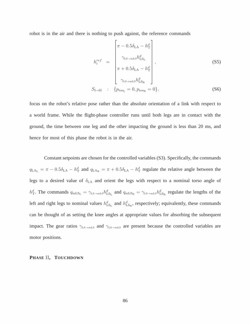
robot is in the air and there is nothing to push against, the reference commands

hrefI

=

π − 0.5δLA − hdT

γLS→mLShdLSL

π + 0.5δLA − hdT

γLS→mLShdLSR

, (S5)

SI→II : {ptoeL = 0, ptoeR = 0}, (S6)

focus on the robot’s relative pose rather than the absolute orientation of a link with respect to

a world frame. While the flight-phase controller runs until both legs are in contact with the

ground, the time between one leg and the other impacting the ground is less than 20 ms, and

hence for most of this phase the robot is in the air.

Constant setpoints are chosen for the controlled variables(S3). Specifically, the commands

qLAL= π − 0.5δLA − hd

T and qLAR= π + 0.5δLA − hd

T regulate the relative angle between the

legs to a desired value ofδLA and orient the legs with respect to a nominal torso angle of

hdT. The commandsqmLSL = γLS→mLSh

dLSL

and qmLSR = γLS→mLShdLSR

regulate the lengths of the

left and right legs to nominal valueshdLSL

andhdLSR

, respectively; equivalently, these commands

can be thought of as setting the knee angles at appropriate values for absorbing the subsequent

impact. The gear ratiosγLS→mLS and γLS→mLS are present because the controlled variables are

motor positions.

PHASE II, TOUCHDOWN

86

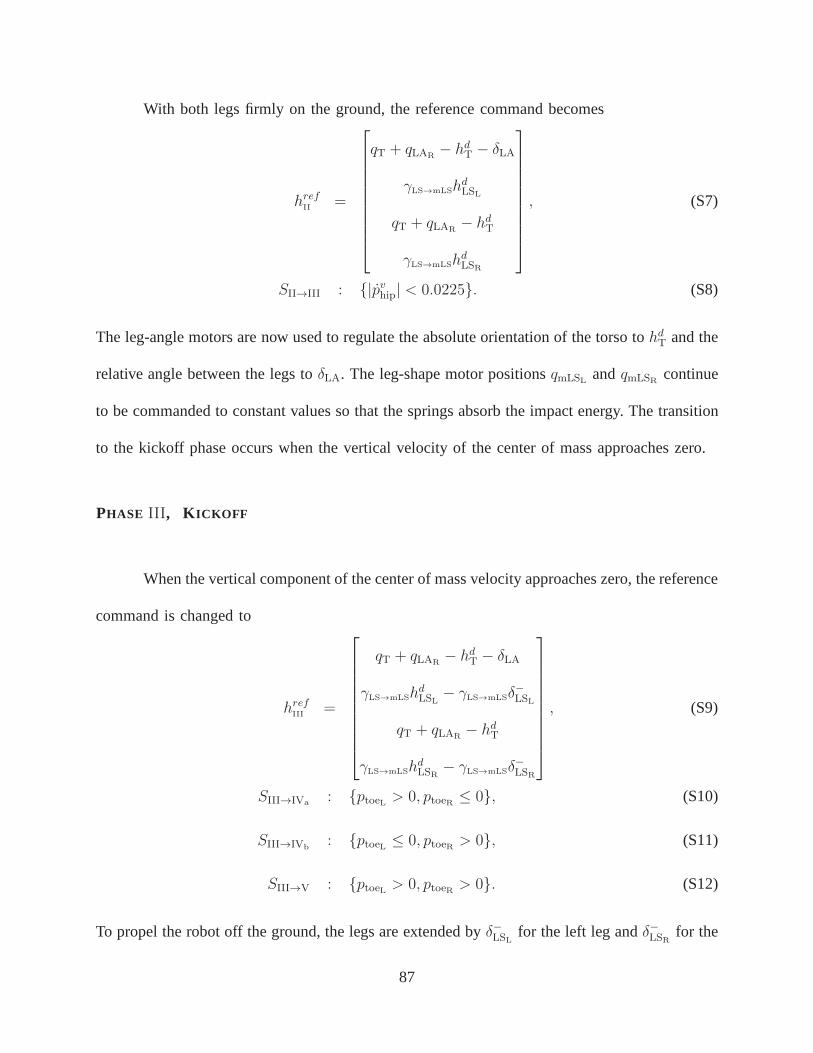
With both legs firmly on the ground, the reference command becomes

hrefII

=

qT + qLAR− hd

T − δLA

γLS→mLShdLSL

qT + qLAR− hd

T

γLS→mLShdLSR

, (S7)

SII→III : {|pvhip| < 0.0225}. (S8)

The leg-angle motors are now used to regulate the absolute orientation of the torso tohdT and the

relative angle between the legs toδLA. The leg-shape motor positionsqmLSL andqmLSR continue

to be commanded to constant values so that the springs absorbthe impact energy. The transition

to the kickoff phase occurs when the vertical velocity of thecenter of mass approaches zero.

PHASE III, K ICKOFF

When the vertical component of the center of mass velocity approaches zero, the reference

command is changed to

hrefIII

=

qT + qLAR− hd

T − δLA

γLS→mLShdLSL

− γLS→mLSδ−

LSL

qT + qLAR− hd

T

γLS→mLShdLSR

− γLS→mLSδ−

LSR

, (S9)

SIII→IVa: {ptoeL > 0, ptoeR ≤ 0}, (S10)

SIII→IVb: {ptoeL ≤ 0, ptoeR > 0}, (S11)

SIII→V : {ptoeL > 0, ptoeR > 0}. (S12)

To propel the robot off the ground, the legs are extended byδ−LSL for the left leg andδ−LSR for the

87

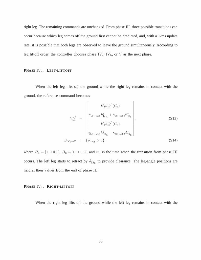
right leg. The remaining commands are unchanged. From phaseIII, three possible transitions can

occur because which leg comes off the ground first cannot be predicted, and, with a 1-ms update

rate, it is possible that both legs are observed to leave the ground simultaneously. According to

leg liftoff order, the controller chooses phaseIVa, IVb, or V as the next phase.

PHASE IVa, LEFT-LIFTOFF

When the left leg lifts off the ground while the right leg remains in contact with the

ground, the reference command becomes

hrefIVa

=

H1hrefIII (t∗

III)

γLS→mLShdLSL

+ γLS→mLSδ+LSL

H3hrefIII (t∗

III)

γLS→mLShdLSR

− γLS→mLSδ−

LSR

, (S13)

SIVa→V : {ptoeR > 0}, (S14)

whereH1 = [1 0 0 0], H3 = [0 0 1 0], and t∗III

is the time when the transition from phaseIII

occurs. The left leg starts to retract byδ+LSL to provide clearance. The leg-angle positions are

held at their values from the end of phaseIII.

PHASE IVb, RIGHT -LIFTOFF

When the right leg lifts off the ground while the left leg remains in contact with the

88

ground, the reference command becomes

hrefIVb

=

H1hrefIII (t∗

III)

γLS→mLShdLSL

− γLS→mLSδ−

LSL

H3hrefIII (t∗

III)

γLS→mLShdLSR

+ γLS→mLSδ+LSR

, (S15)

SIVb→V : {ptoeL > 0}. (S16)

The notation is as in phaseIVa. The right leg starts to retract byδ+LSR to provide clearance. The

leg-angle positions are held at their values from the end of phaseIII.

PHASE V, RETRACT

Once both legs lift off the ground, the retraction phase is held for 50 ms, after which the

controller passes to the flight phase. The reference commandis

hrefV

=

H1hrefIII (t∗

III)

γLS→mLShdLSL

+ γLS→mLSδ+LSL

H3hrefIII (t∗

III)

γLS→mLShdLSR

+ γLS→mLSδ+LSR

, (S17)

SV→I : {t = t#V+ 0.05}, (S18)

where t#V is the time when the transition to phaseV occurs. Otherwise, the notation is as in

phaseIVa. The leg-angle positions are held at their values from the end of phaseIII. Both legs

are retracted to provide clearance.

PARAMETER VALUES

89

Applying the above controller to the identified model, a periodic solution is found with

the controller parameter values

δLA = 0.524 rad (30 deg), hd0T = 0.140 rad (8 deg),

hdLSL

= 0.209 rad (12 deg), hdLSR

= 0.209 rad (12 deg),

δ−LSL = 0.087 rad (5 deg), δ−LSR = 0.227 rad (13 deg),

δ+LSL = 0.087 rad (5 deg), δ+LSR = 0.087 rad (5 deg),

with the robot’s horizontal position over one hop translated backward by0.27 m, which

corresponds toδφdh = −0.273 rad = −6.9 deg of rotation as measured by the encoder on

the central tower.

Simulation shows that the periodic motion is unstable. The orbit is stabilized with an

event-based controller that updates the commanded torso anglehdT based on the distance traveled

horizontally during one hop, namely,

φh[k] = φh (tI→II) ,

δhdT[k] = KT(φh[k]− φh[k − 1]− δφd

h),

hdT[k] = hd0

T + δhdT[k],

wherek is the hopping count,tI→II is the time when the transition from phase I to phase II

occurs, andKT is a gain. If MABEL travels less thanδφdh during the previous hop, the torso is

leaned backward from the nominal valuehd0T , and vice versa if the robot travels more thanδφd

h.

A few hours of parameter tuning with the simulation model resulted in a stabilizing

controller, while days of trial and error in the laboratory were unsuccessful.

90

Flight

Touchdown

KickoffLeft-liftoff

Right-liftoff

Retract

SI→II

SII→III

SIII→IVb

SIII→IVa

SIII→VSIVa→V

SIVb→V

SV→I

Figure S3: Hopping controller phases and transitions. Fromphase III, three possible transitions

can occur because which leg first comes off the ground cannot be predicted. According to which

leg comes off the ground, the controller selects phaseIVa, IVb, or V as the next phase.

91

AUTHOR BIOGRAPHIES

Hae-Won Park (Corresponding Author) (parkhw@umich.edu) is a Ph.D. candidate in the

Department of Mechanical Engineering, the University of Michigan, Ann Arbor. He received the

B.S. and M.S. degrees in mechanical engineering from YonseiUniversity, Seoul, South Korea

in 2005 and 2007, respectively. He started his doctorate at the University of Michigan in 2007.

His research interests are in modeling, system identification, and control of robotic systems. He

can be contacted at 1303 Beal Ave., 4303 EECS Building, University of Michigan, Ann Arbor,

Michigan 48109-2111, USA.

Koushil Sreenath is a Ph.D. candidate in the Electrical Engineering and Computer Science

Department at The University of Michigan, Ann Arbor. He received the B.E. from PES Institute

of Technology, Bangalore, India in 2002, and the M.S. from The University of Texas, Arlington

in 2005. From 2006 to 2007, he was a Research Engineer with theIntelligent Controls Group,

Saint-Gobain R&D, Northboro, MA. His research interests are in modeling, feedback design,

and experiments in legged robotics, as well as adaptive sampling and resource allocation in

mobile wireless sensor networks.

Jonathan Hurst is an assistant professor of Mechanical Engineering at Oregon State

University. He received the B.S. degree in mechanical engineering, the M.S. in robotics, and

the Ph.D. in robotics from Carnegie Mellon University, Pittsburgh, PA, in 2001, 2004 and 2008,

respectively. He designed and built MABEL while a Ph.D student. His research interests include

legged locomotion, natural dynamics, and robot actuation,with special interest in the role and

implementation of compliance in legged locomotion.

92

Jessy W. Grizzle is a professor of Electrical Engineering and Computer Science at The

University of Michigan, Ann Arbor, where he also holds the Jerry and Carol Levin professorship.

He is a Fellow of the IEEE. He jointly holds sixteen patents dealing with emissions reduction

in passenger vehicles through improved control system design. His work on bipedal locomotion

has been presented in numerous plenary lectures and has beenfeatured in The Economist, Wired

Magazine, Discover Magazine, Scientific American, and several television programs.

93