Parallel Numerical Solution of the 2D Heat · PDF fileIntroduction Heat equation Existence...

IntroductionHeat equation

Existence uniquenessNumerical analysis

Numerical simulationConclusion

Parallel Numerical Solution of the 2D HeatEquation

Lydia Flore Mamoade

16 January 2012

Lydia Flore Mamoade Parallel Numerical Solution of the 2D Heat Equation




Table of contents

1 Introduction

2 Heat equation

3 Existence uniqueness

4 Numerical analysis

5 Numerical simulation

6 Conclusion





Introduction

Aim: parallel solving of the heat equation with MPI.





Basic equation

Figure: ⌦ = [0, Lx ]⇥ [0, Ly ]





Basic equation

8>>><

>>>:

@u(x , y , t)

@t�D4u(x , y , t) = f (x , y , t) in ⌦

u = g(x , y , t) on �0

u = h(x , y , t) on �1

u(x , y , 0) = u0(x , y)

(1)

where @⌦ = �0 [ �1, @⌦ is the boundary of ⌦, t 2 [0,T ] ⇢ R andx,y 2 ⌦. D > 0We assume that, u0 2 L2(⌦), f 2 L2([0,T ],L2(⌦)),

and we suppose g 2 H12 (�0), h 2 H

12 (�1),





Existence, uniqueness:

Existence and uniqueness of the continuous solution is provedusing the spectral method.

Proof.

For the proof, we refer to the report.





Implicit Euler scheme

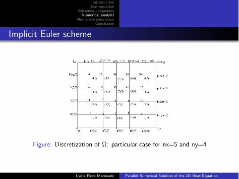
Figure: Discretization of ⌦: particular case for nx=5 and ny=4






Spacial mesh points: xj

= j�x and yi

= i�y, 1 j nx and

1 i ny, where �x =L

x

(nx + 1), �y =

Ly

(ny + 1).

Temporal mesh points: t = n�t. 1 n nt.

Value of u at the point (xj

, yi

) and at time tn

:un

ji

= u(xj

, xi

, tn

).






At the point (xj

, yi

) and at time tn

the original di↵erential equation(1) becomes:u

n

j,i�u

n�1j,i

�t � D⇣

u

n

j�1,i�2u

n

j,i+u

n

j+1,i

�x2 +u

n

j,i�1�2u

n

j,i+u

n

j,i+1

�y2

⌘= f n

j ,i in ⌦

u = gn

j ,0 on �s

0 u = gn

j ,ny+1 on �n

0

u = hn

0,i on �w

1 u = hn

nx+1,i on �e

1






We define the global notation l = (i � 1)nx + j this is equivalent toi = [ l�1

nx

+ 1] and j = mod(l � 1, nx) + 1.

un

l

� un�1l

�t�D

✓un

l�1 � 2un

l

+ un

l+1

�x2+

un

l�nx

� 2un

l

+ un

l+nx

�y2

◆= f n

l

in ⌦

(2)

l =

8>><

>>:

1, . . . , nx on �s

0

nx(ny � 1) + p p = 1, . . . , nx on �n

0

(p � 1)nx + 1 p = 1, . . . , ny on �w

1

pnx p = 1, . . . ny on �e

1





Convergence

We define Lap

u:

un

j ,i � un�1j ,i

�t�D

✓un

j�1,i � 2un

j ,i + un

j+1,i

�x2+

un

j ,i�1 � 2un

j ,i + un

j ,i+1

�y2

◆= f n

j ,i

Using Taylor expansion one can show that the implicit Eulerscheme is of order 2 in space and of order 1 in time.





Linear System

We write the system (2) in matrix form AU=F.





Structure of the matrix A

A in the case where nx=5 and ny=4

A =

0

BB@

C B 0 0B C B 00 B C B0 0 B C

1

CCA

where 0 is the nx by nx 0 matrix,

C =

0

BBBB@

a b 0 0 0b a b 0 00 b a b 00 0 b a b0 0 0 b a

1

CCCCA

and B=cI5 with a = 1 + 2�tD�x2 + 2�tD

�y2 , b = � �tD�x2 and c = � �tD

�y2 .





Properties of the matrix A

The matrix A in (13) is real, symmetric, positive-defined and hasstrictly dominant diagonal since|A

i ,j | >P

j 6=i

Ai ,j for all i. Therefore A is invertible, hence AU=F

has a solution, that we will compute numerically using conjugategradient method.





conjugate gradient Algorithm

r0 := B � AX0

p0 := r0k := 0repeat

↵k

:=r

t

k

r

k

p

t

k

Ap

k

Xk+1 := X

k

+ ↵k

pk

rk+1 := r

k

� ↵k

Apk

if rk+1 is su�ciently small then exit loop end if

�k

:=r

t

k+1rk+1

r

t

k

r

k

pk+1 := r

k+1 + �k

pk

end repeatk := k + 1





Parallelization

We are going focus on the parallelization of the operator A, wedivide the rows of the matrix A between the processors. Eachprocessors knows a peace of the vector of unknowns U.





Parallel Algorithm

1.Initializationstime loop2. construction of second member3. resolution of linear system : conjugate gradientmatrix vector productsscalar productcombinations of linear of vectors4. progression in timeFinalizations :destruction of MPI environmentsdeallocation of the matrix and vectorsThe big work here in this algorithm is the parallelization of thematrix vectors product.





Matrix vector products: Communication

In order to do the matrix vector products the processors mustcommunicate, their results two to two, so we use point-to-pointcommunication MPI SEND and MPI RECV. In fact the processorme must know the nx last values of the vector solution of theprocessor me +1 and the ns first values of the vector solution.





scalar product:reduction

Each processor do the simple scalar product of the peaces of thevectors they have, we use MPI ALLREDUCE to make the sum ofelementary result, and transmit the result to all processors.





Illustration

To illustrate the problem we consider three di↵erent cases.For the first two cases we checked the correlation between thenumerical solution and exact one.





Illustration: stationary case 1

f (x , y) = 2(x � x2 + y � y2) g(x , y) = 0 h(x , y) = 0.Exact solution u(x , y) = xy(1� x)(1� y).

Figure: Numerical solution of stationary case 1 for nx=25 et ny=25 withfive processors.





Illustration: stationary case 2

f (x , y) = sin(x) + cos(y) g(x , y) = sin(x) + cos(y)h(x , y) = sin(x) + cos(y).Exact solution u(x , y) = sin(x) + cos(y).

Figure: Numerical solution of stationary case 2 for nx=25 et ny=25 withfive processors





Illustration: instationary case

f (x , y) = exp(�(x�Lx

2)2) exp(�(x�L

x

2)2) g(x , y) = 0 h(x , y) = 1.

Figure: Numerical solution of instationary case for nx=25 et ny=25 withfive processors. Lydia Flore Mamoade Parallel Numerical Solution of the 2D Heat Equation




Speedup

Speedup =Computing time of sequential code

Computing time of Parallel code

Figure: Graphs of speed up of both stationary cases and of instationarycase against the number of processors for nx=160, ny=160.





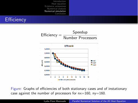
E�ciency

E�ciency =Speedup

Number Processors

Figure: Graphs of e�ciencies of both stationary cases and of instationarycase against the number of processors for nx=160, ny=160.





Conclusion

speed-up given in Figure [24] increases very slowly when thenumber of processors increases, with this speed-up we get ane�ciency of 20% which is not very e�cient, but acceptable.





END

End

THANK YOU FOR YOUR ATTENTION !!!!!


Parallel Numerical Solution of the 2D Heat · PDF fileIntroduction Heat equation Existence...

Documents

Transcript of Parallel Numerical Solution of the 2D Heat · PDF fileIntroduction Heat equation Existence...