PARALLEL ALGORITHMS FOR NEAREST …padas.ices.utexas.edu/static/papers/knn.pdfPARALLEL ALGORITHMS...
33
PARALLEL ALGORITHMS FOR NEAREST NEIGHBOR SEARCH PROBLEMS IN HIGH DIMENSIONS. BO XIAO * AND GEORGE BIROS † Abstract. The nearest neighbor search problem in general dimensions finds application in com- putational geometry, computational statistics, pattern recognition, and machine learning. Although there is a significant body of work on theory and algorithms, surprisingly little work has been done on algorithms for high-end computing platforms and no open source library exists that can scale efficiently to thousands of cores. In this paper, we present algorithms and a library built on top of Message Passing Interface (MPI) and OpenMP that enable nearest neighbor searches to hundreds of thousands of cores for arbitrary dimensional datasets. The library supports both exact and approximate nearest neighbor searches. The latter is based on iterative, randomized, and greedy KD-tree searches. We describe novel algorithms for the con- struction of the KD-tree, give complexity analysis, and provide experimental evidence for the scal- ability of the method. In our largest runs, we were able to perform an all-neighbors query search on a 13 TB synthetic dataset of 0.8 billion points in 2,048 dimensions on the 131K cores on Oak Ridge’s XK6 “Jaguar” system. These results represent several orders of magnitude improvement over current state-of-the-art methods. Also, we apply our method to non-synthetic data from machine learning data repositories. For example, we perform an all-nearest-neighbor search on a variant of the ”MNIST” handwritten digit dataset with 8 million points in 784 dimensions on 16,384 cores of the ”Stampede” system at the Texas Advanced Computing Center, achieving less than one second per PKDT iteration. Key words. Nearest Neighbor Algorithms, Computational Statistics, Tree Codes, Data Anal- ysis, Parallel Algorithms, Machine Learning AMS subject classifications. 65N30, 65N50, 65N55, 65Y05, 68W10, 68W15 1. Introduction . Given a set R of n reference points {r i } n i=1 ∈ R d , and a distance metric d(r i , r j ) (e.g., the Euclidean metric kr i - r j k 2 ), we seek to find the k- nearest neighbors (KNN) for points {q i } m i=1 ∈ R d from a query points set Q. When the query points are the same as the reference points, KNN is commonly refer to as the all nearest neighbors problem. Solving the k-nearest neighbors problem is easy by direct search in O(mn) work. That is, for each query point all distances to the reference points are evaluated followed by a k-selection problem in a list of n numbers. The all-KNN problem requires O(n 2 ) work, which is prohibitively expensive when n is large. Spatial data structures can deliver O(n log n) or even O(n) complexity, asymptotically, for fixed dimension d. But for high dimensions (say, d ≥ 10), spatial data structures provably deteriorate; for large d all known exact schemes end up having the complexity of the direct algorithm [47]. 1 In many applications however, the distribution of points is mostly concentrated in a lower-dimensional subspace of R d . In such cases, find approximate nearest neighbors (ANN) using indexing techniques (tree-type data structures or hashing techniques) can be more realistic than direct searches. For each query point q i , ANN attempts to find some points r j that have high probability to be the k closest points in the given metric. Those that are not among the ”exact” nearest neighbors are close to being so. In the following of this paper, we refer to the exact k-nearest neighbors search * The University of Texas at Austin, Institute for Computational Engineering and Sciences, Austin, TX 78712 ([email protected]). † The University of Texas at Austin, Institute for Computational Engineering and Sciences, Austin, TX 78712 ([email protected]). 1 An easy way to see why is to consider a lattice of points. Every point has 2 d immediate neighbors. 1
Transcript of PARALLEL ALGORITHMS FOR NEAREST …padas.ices.utexas.edu/static/papers/knn.pdfPARALLEL ALGORITHMS...

PARALLEL ALGORITHMS FOR NEAREST NEIGHBOR SEARCHPROBLEMS IN HIGH DIMENSIONS.
BO XIAO∗ AND GEORGE BIROS†
Abstract. The nearest neighbor search problem in general dimensions finds application in com-putational geometry, computational statistics, pattern recognition, and machine learning. Althoughthere is a significant body of work on theory and algorithms, surprisingly little work has been doneon algorithms for high-end computing platforms and no open source library exists that can scaleefficiently to thousands of cores. In this paper, we present algorithms and a library built on top ofMessage Passing Interface (MPI) and OpenMP that enable nearest neighbor searches to hundreds ofthousands of cores for arbitrary dimensional datasets.
The library supports both exact and approximate nearest neighbor searches. The latter is basedon iterative, randomized, and greedy KD-tree searches. We describe novel algorithms for the con-struction of the KD-tree, give complexity analysis, and provide experimental evidence for the scal-ability of the method. In our largest runs, we were able to perform an all-neighbors query searchon a 13 TB synthetic dataset of 0.8 billion points in 2,048 dimensions on the 131K cores on OakRidge’s XK6 “Jaguar” system. These results represent several orders of magnitude improvement overcurrent state-of-the-art methods. Also, we apply our method to non-synthetic data from machinelearning data repositories. For example, we perform an all-nearest-neighbor search on a variant ofthe ”MNIST” handwritten digit dataset with 8 million points in 784 dimensions on 16,384 cores ofthe ”Stampede” system at the Texas Advanced Computing Center, achieving less than one secondper PKDT iteration.
Key words. Nearest Neighbor Algorithms, Computational Statistics, Tree Codes, Data Anal-ysis, Parallel Algorithms, Machine Learning
AMS subject classifications. 65N30, 65N50, 65N55, 65Y05, 68W10, 68W15
1. Introduction . Given a set R of n reference points {ri}ni=1 ∈ Rd, and adistance metric d(ri, rj) (e.g., the Euclidean metric ‖ri− rj‖2), we seek to find the k-nearest neighbors (KNN) for points {qi}mi=1 ∈ Rd from a query points set Q. When thequery points are the same as the reference points, KNN is commonly refer to as the allnearest neighbors problem. Solving the k-nearest neighbors problem is easy by directsearch in O(mn) work. That is, for each query point all distances to the referencepoints are evaluated followed by a k-selection problem in a list of n numbers. Theall-KNN problem requires O(n2) work, which is prohibitively expensive when n is large.Spatial data structures can deliver O(n log n) or even O(n) complexity, asymptotically,for fixed dimension d. But for high dimensions (say, d ≥ 10), spatial data structuresprovably deteriorate; for large d all known exact schemes end up having the complexityof the direct algorithm [47].1
In many applications however, the distribution of points is mostly concentrated ina lower-dimensional subspace of Rd. In such cases, find approximate nearest neighbors(ANN) using indexing techniques (tree-type data structures or hashing techniques) canbe more realistic than direct searches. For each query point qi, ANN attempts to findsome points rj that have high probability to be the k closest points in the givenmetric. Those that are not among the ”exact” nearest neighbors are close to beingso. In the following of this paper, we refer to the exact k-nearest neighbors search
∗The University of Texas at Austin, Institute for Computational Engineering and Sciences, Austin,TX 78712 ([email protected]).†The University of Texas at Austin, Institute for Computational Engineering and Sciences, Austin,
TX 78712 ([email protected]).1An easy way to see why is to consider a lattice of points. Every point has 2d immediate
neighbors.
1

2 B. XIAO, AND G. BIROS
problem as KNN, and the approximate nearest neighbors search problem as ANN. Thispaper mainly focus on a scheme that uses tree indexing to solve ANN.
Motivation and significance. The KNN problem is a fundamental problemthat serves as a building block for higher-level algorithms in computational statistics(e.g., kernel density estimation), spatial statistics (e.g., n-point correlation functions),machine learning (e.g., classification, regression, manifold learning), high-dimensionaland generalized N-body problems, dimension reduction for scientific datasets, anduncertainty estimation [13, 41, 38]. Examples of the applicability of these methods toscience and engineering include image analysis and pattern recognition [45], materialsscience [15], cosmological applications [18], particulate flow simulations [36], and manyothers [1]. Despite nearest neighbors search being fundamental for many algorithmsin computational data analysis, there is little work on scaling it to high-performanceparallel platforms.
1.1. Our approach and contributions. We introduce algorithms, complex-ity analysis, and experimental validation for tree-construction and nearest neighborsearches in arbitrary dimensions.
• Direct nearest neighbors. We propose two parallel algorithms for the directcalculation of the KNN problem. The first one prioritizes computing timeover memory by replicating the query and reference points while minimizingthe synchronization costs. This method is useful when absolute wall-clockperformance is important. It is work-, but not memory-, optimal. The sec-ond algorithm uses a cyclic iteration that is memory optimal but has morecommunication. Both algorithms can be used for modestly-sized datasets tocompute exact distances and verify correctness of approximate algorithms.But since the perform direct evaluations they cannot scale with m and n.
• Parallel tree construction. We present PKDT, a set of parallel tree constructionalgorithms for indexing structures in arbitrary number of dimensions. Thealgorithm supports several types of trees (e.g., ball trees, metric trees, or KD-trees). It is a recursive, top-down algorithm in which every node correspondsto a group of processes and one group of reference points. The key feature ofthe algorithm is that the tree is not replicated across MPI ranks. The tree isused to partition and prune spatial searches across MPI processes.
• Approximate randomized nearest-neighbor searches. We present a randomizedtree algorithm based on PKDT, randomization, and iterative greedy searches,for the solution of the ANN problem. Our implementation supports arbitraryquery and reference points. We test the accuracy on both synthetic andmachine-learning benchmark datasets and we report the results in §3.3. Weare able to obtain good accuracies with less than 5% of the distance evalua-tions required for an exact search.
• Scalability tests on up to 131K cores. We conduct weak and strong scalabilitytests for the various components of the method. The largest run is up tonearly one billion 2048-dimensional reference points for the ANN problem fork = 2048. This result dwarfs the previously reported result with one millionpoints in 10 dimensions for k = 3 [8] (see §3.4). Table 1.1 summarizes thelargest data size we run on each method.
• Software release. We make this software available as part of a library forscalable data analysis tools. The library is under the GNU General PublicLicense, it is open-source, available at RKDT. The library supports hierarchicalkmeans trees, ball trees, KD trees, exact and approximate nearest neighbor

FAST KNN ALGORITHMS 3
searches, and kmeans clustering with different seeding variants.
data sizeKNN ANN
2d partition cyclic partition PKDT randomized PKDT
number of points (million) 82 12 160 819
dimension 1,000 100 100 2,048
number of processes 16,384 12,288 12,288 16,384
million cycles/point/core 12 266 1 40
Table 1.1Overall performance summarization of different nearest neighbors search. We listed the latest
data sizes in our experiments for each methods, for which the all nearest neighbors are selected.
To our knowledge, our framework is the first scheme that enables such levels ofperformance and parallelism for arbitrary dimension computational geometry prob-lems. Our tree construction and nearest-neighbors are already being used for kernelsummation and treecodes in high dimensions [24, 25].
1.2. Limitations. PKDT has several limitations: (1) It has not be designed forfrequent insertions or deletion of points. (2) PKDT does not resolve the curse of dimen-sionality. If the dataset has high intrinsic dimension, the approximation errors willbe very large. (3) We have only examined `2 distance metrics and many applicationsrequire other distance metrics. However, this is a simple implementation issue, atleast for standard distance metrics.
1.3. Related work. There is a very rich literature on nearest neighbor algo-rithms and theory. The most frequently used algorithm is the KD-tree [12], which ateach level partitions the points into two groups according to one coordinate. Fuku-naga et al [14] propose another tree structure that groups points by clustering pointswith kmeans into k disjoint groups. If the metric is non Euclidean, however, ball treeor metric tree might provide better performance [7, 46, 31]. As the dimensionalityincreases, each of these methods lose their effectiveness quickly, requiring visit almostall leaf nodes in a tree. In fact in high-dimensional spaces there are no known algo-rithms for exact nearest neighbor search that are more efficient than the direct exactsearch (or linear search per query point). Modern implementations of exact searchesinclude [18, 37, 8, 27].
Avoiding this curse of dimensionality requires two ingredients. The first is tosettle for approximate searches. The second is to introduce the assumption that thedataset has a lower intrinsic dimensionality, i.e., the dataset points lie on a lowerdimensional subspace of Rd [20, 35, 6]. Given this, the search complexity per querypoint can be theoretically reduced from O(n) to O(η log n), where η is determinedonly by the intrinsic dimensionality of data points [44, 39, 5, 9]. Several approxi-mate algorithms have been proposed, with their main theoretical result being that,asymptotically, they can bound the relative error in the distance from the true nearestneighbor. No algorithm offers an actual practical accuracy guarantee, while simulta-neously bounding the work complexity. There are two main classes of approximations,randomized tree based and hashing based algorithms.
Randomized tree algorithms were first proposed in [9]. Different variants of thisapproach have been used for the KNN problem: [30, 2, 19, 28]. In this paper we followthe work of [19]. Another tree-based algorithm, without randomization, that supportsapproximate KNN by pruning the tree search is presented in [27].

4 B. XIAO, AND G. BIROS
A different approach to approximate is KNN is to use hashing. Locality sensitivehashing (LSH) bins the reference points so that similar points are grouped into thesame bucket with high probability. The details of the LSH algorithm can be foundin [5]. The original implementation of LSH can be found in [4]. In [33], the au-thors present excellent analysis and implementation of the LSH algorithm on a GPUarchitecture. No open-source LSH based algorithms for HPC distributed memory ar-chitectures are available. We have implemented an MPI LSH algorithm, and we willdiscuss its comparison with randomized trees in a future article.
Scalability and available software. As we mentioned there is little on dis-tributed memory scalable algorithms for nearest-neighbor searches. Also, while thereis excellent theoretical work on parallel KD-tree construction [3], no implementationsare available. Nearest neighbor algorithms using direct search or LSH on GPUs can befound in [16, 42, 34, 17]. The one exception is the FLANN package [30, 28], which sup-ports multithreading and some MPI based parallelism in which the reference pointsare partitioned across processors and the query points are replicated. In [30] no all-KNN results are presented for the MPI version, and runs are done only up to eightnodes and for very small m (number of query points). FLANN’s MPI parallel schemeresembles the scheme described in §2.2.1 but with approximate searches. This schemedoes not scale well for the all-KNN problem as it requires replication of the query seton each MPI process. Other open-source libraries include MLPACK [8] and ANN [27].These libraries do not support distributed memory parallelism. We discuss more theperformance of these codes and FLANN in §3.4. In all, to the best of our knowledge,no scalable KNN libraries exist.
Outline of the paper. In §2, we introduce the basic algorithmic components ofthe method: the single node optimization of distance calculations and KNN search(shared memory parallelization) (§2.1); two schemes for direct exact parallel KNN
search (§2.2.1 and §2.2.2); and our main contribution, the parallel tree constructionand ANN search in §2.3. In §3, we apply our KNN algorithms on large UCI datasets [22]and discuss the relationship between the convergence and the intrinsic dimensions.Finally, we report more results on the performance and scalability of the method onvery large synthetic datasets.
2. Methods. We have implemented several scalable methods for both KNN andANN. In the following sections, we discuss the different components and we provideweak and strong scaling results.
2.1. Single-node distance and k-nearest neighbor kernels. We use single-node, multi-threaded kernels for both distance calculations and KNN searches on locallystored points. The distances between all (qi, rj) pairs of points are computed asfollows. The sets of reference points R and query points Q are stored as n × d andm × d matrices, respectively, with one point per row. Then, we compute Dij =|qi|2 + |rj |2 − 2ri · qj for all (i, j), i ∈ 1 . . .m, j ∈ 1 . . . n, where Dij is the square ofthe distance between query point i and reference point j. By expressing the −2ri ·qjterm as the matrix-matrix product −2RQT , we can use a BLAS DGEMM call, whichdelivers high single-node performance and portability to various homogeneous andheterogeneous platforms.
With the above squared-distance kernel, a single-node KNN calculation is quitesimple. It can be implemented by calling the above distance routine and, for eachquery point, sorting the squared distances in ascending order while keeping track ofthe index of the reference point corresponding to each distance. Clearly, this approachexposes a great deal of parallelism. However, for sufficiently small k (k << n), we

FAST KNN ALGORITHMS 5
would waste a significant amount of time by sorting each row of D in its entirety. Sincewe only care about the first k nearest points, we address this problem by maintaining aminimum heap of size k for each query point. Scanning the n reference points requiresinserting every reference point into the minimum heap at a cost of O(log k). Thusthe total complexity is O(n log k), which is less expensive than a sort of O(n log n).
One implementation issue encountered in the development of the direct KNN ker-nel involves the fact that vendor tuned DGEMM routines provide very poor multi-threaded performance when multiplying a tall, skinny matrix by a relatively smallmatrix. In our code, this happens when computing distances between a small numberof query points and a large number of reference points with low dimensionality. Wehave observed this problematic behavior in both Intel’s MKL and GOTO BLAS. Weare currently addressing this problem by developing a customized high performancekernel for nearest neighbor searches, which achieves more uniform performance. Thoseresults will be reported elsewhere.
2.2. Brute-force Direct KNN. We have implemented two distributed directevaluation (brute-force) nearest neighbor algorithms according to different data par-tition schemes: two-dimensional partitioning and cyclic partitioning.
2.2.1. Two dimensional partitioning with query point replication. Wefirst consider a partitioning scheme in which the reference and query points are dividedinto rparts and qparts pieces, respectively, and distributed across rparts · qparts nodes(see Figure 2.1(a)). This scheme is more memory-intensive than the cyclic partitioningscheme we describe later since the reference points and the query points are replicatedqparts and rparts times, respectively. However, all calculations performed are local untila reduction at the very end.
Algorithm 1 rectDirectK(nglobal,mglobal, k, d, rparts, qparts)
1: Choose nlocal and mlocal.2: Read nlocal reference points into rlocal starting with dnglobal/rpartse · id.3: Read mlocal query points into qlocal starting with dmglobal/qpartse · id.4: D = computeDistances(rlocal,qlocal, nlocal,mlocal, k, dim)5: for i = 0 . . . qparts − 1 do Sort ith row of D6: Perform k-reduction among processes with ranks id%qparts, id%qparts +qparts, . . . , id%qparts + (rparts − 1) · qparts.
7: Process has k-nearest neighbors for qlocal if id < qparts.
Algorithm 1 shows how this partitioning is used to compute the KNN. Each pro-cess computes a matrix containing the distance between each (ri,qj) pair, and sortseach row of the matrix (the distances for each query point) to select the k minimumdistances. Finally, we perform a k-min reduction among all processes which have thesame query points.
Assuming the query and reference points are partitioned into an equal numberof pieces, each process’s memory consumption grows as O( n√
p + m√p + nm
p ), since
each set of points is replicated√p times. Since our algorithm requires an all-pairs
distance calculation, a sort of the computed distances (selection sort for small k andmerge sort for large k), and a reduction on the k minimum of those distances, its
time complexity is O(mndp + 1√
p (m + n) + mnp (log n√
p ) + k log√p
)for large k, and

6 B. XIAO, AND G. BIROS
O(mndp + 1√
p (m+ n) + mnp + k log
√p
)for small k.
(a) Rectangular partitioning (b) Cyclic partitioning
Fig. 2.1. Data partition for direct search. (a) Diagram of rectangular partitioning. Here thequery points are partitioned into four parts and the reference points into three. The processes in eachcolumn are part of the same group when the k-reduction is performed at the end of the algorithm.Depending on the mapping to MPI processes, the query points, the reference points, or both arereplicated (b) Diagram of cyclic partitioning. Notice that now there is no replication but the methodrequires four steps and cyclic-shift of the query or reference points, depending on which one is ofsmaller cardinality.
2.2.2. Cyclic partitioning for large problem sizes. By using a partitioningscheme that does not replicate any data across processes, we can solve the exact KNN forsignificantly larger problem sizes than would fit into a single nodes’s memory whenusing the replicated partitioning scheme. However, the reduced memory footprintcomes at the cost of additional computation time. As illustrated in Figure 2.1(b),in this method, both R and Q are partitioned into p nearly-equally sized partitionsdistributed among the processes.
Algorithm 2 shows how to use such a partitioning to compute the k-nearest neigh-bors. The algorithm works as follows. A given partition of Q remains pinned to its“home” process, while in each of p communication steps, each partition of R shiftsone process to the left in a “ring” of processes. At each communication step, a processruns the local direct KNN kernel and merges the results with the current k minimumdistances for each query point. Depending on which set is larger, we can cycle eitherthe reference points or the query points.
The communication cost of this algorithm is O(ptS +ndtT ), where tS is the setuptime (latency) required for each message, and tT is the time required to transmit eachdouble-precision value. Because communication and computation can be overlappedcompletely for sufficiently large m and n, the time complexity is determined by thetime spent in the local direct KNN calculation, which is O(mndp +m+n+ mn
p log np ) for
large k and O(mndp +m+ n+ mnkp ) for small k. The memory cost for this approach
is O(mn+m+np ).
2.3. Randomized KD tree (PKDT). Parallelizing tree operations with perfor-mance guarantees depends on the application and is hard even in low dimensions,especially in distributed memory architectures. Most of the tree algorithms for highdimensions follow a top-down approach in which the points are grouped recursivelyinto tree nodes and then, during search, different pruning strategies are used [40].Other techniques such as space-filling curves [21], graph partitioning [10] and geo-metric partitioning [26] have been used for parallelization, but for high-dimensionaldatasets these are not as successful and we are not aware of any parallel implementa-tions. For this reason we have opted for the top-down basic approach.

FAST KNN ALGORITHMS 7
Algorithm 2 cyclicDirectK(r, q, nglobal,mglobal, k, dim)
1: Choose send partner and recv partner.2: for i = 0 . . . p− 1 do3: if kmin set then4: kmin new ← directKQuery(Ri,Qi, nlocal,mlocal, k, d)5: temp← kmin merge(kmin, kmin new,mlocal, k)6: kmin← temp7: else8: kmin← directKQuery(Ri,Qi, nlocal,mlocal, k, d)9: kmin set← TRUE
10: end if11: send(r, send partner)12: r ← recv(recv partner)13: end for14: send(r, send partner)15: r ← recv(recv partner)
Fig. 2.2. Hyperplane splitting. An illustration of the hyperplane splitting.
Forgetting parallelism for a moment, the basic algorithm is a classical top-downrecursive construction of a binary tree. Starting at the root. We split the points intotwo groups, and create two new nodes (the left and right child of the root). Thenwe assign one group of points to one child and the other group to the other child.We compared two point splitting schemes: clusters based (refered as PKDTC) andhyperplane based (refered as PKDTH).
In PKDTC , we use kmeans with a large number of clusters (greater than two, sothat we can control the number of points per leaf node) and then we assign clustersto different nodes. Hyperplane splitting is quite common and includes standard KD-trees. Clustering is used in FLANN [30, 29] and we want to test its performance. Theclustering algorithm is given in the appendix. The hyperplane splitting is illustratedin Algorithm 3 and Figure 2.2.
In a hyperplane based scheme, we calculate a projection direction and projectall points onto this direction, then split the points according to the median of theprojected values. We tested three ways to choose the projection direction. Thefirst one is selecting a coordinate axis at random, i.e., uniformly sampling a numberfrom d integers. The second is to choose the coordinate with the largest varianceconsidering all points within a node. The third alternative is to choose the direction

8 B. XIAO, AND G. BIROS
where the points are furthest apart. To do this, we first compute the centroid c of allpoints within a node, then find the furthest point p1 from c, and a second point p2
which is furthest from p1. Finally we project points along the direction p = p1 −p2.After projecting points onto this direction and calculate the median m of all projectedvalues, we simply separate points into two groups by assigning points whose projectedvalues is smaller than m to the left child, and the other to the right child. All of thesethree resulted in similar accuracies when used for the ANN problem. For the rest of thispaper, the complexity estimates are computed using the random selection criterion.
In the end we found the hyperplane partition superior. First, partitioning pointsevenly using a hyperplane results in roughly the same number of points per group,which has implications to the parallel implementation and the load balancing of thealgorithm. In other words, each child node has the same number of points as theothers. Second, clustering based partition is more expensive as it requires solvingkmeans problems multiple times. Third, we observe that the hyperplane splittingresults in better pruning during neighbor searches. In the following parts, we onlyfocus on PKDTH , and the details of PKDTC can be found in Appendix B.
2.3.1. Tree construction. A standard tree construction uses the NodeSplitfunction summarized in Algorithm 3. Let T be a tree node; XT be all the pointsassigned to T , lT be the level of the node T in the tree. Hyperplane splitting requiresa direction pT along which XT are projected. mT is the median of all projected valuesxpT . Denote Xl and Xr as the subset of XT , which contains the points assigned tothe left child node and right child node of T respectively. For bookeeping we usea maxLevel setting to indicate the maximum allowed level of a node and we useminNumofPoints (minimum number of points a node have to hold) to decide whetherto split a node further or not.
Algorithm 3 NodeSplit(T , XT )
1: if lT ==maxLevel || |XT | < minNumofPoints then2: store XT in T3: return4: end if5: pT = SplitDirection(T ,XT )6: xpT = Project(XT ,pT )7: mT = Median(xpT )8: for xi ∈ XT do9: if xpT ,i < mT then
10: assign xi to Xl
11: else12: assign xi to Xr
13: end if14: end for15: NodeSplit(LeftChild(T ),Xl)16: NodeSplit(RightChild(T ),Xr)
Shared memory PKDTH construction: Building a shared memory tree isstraightforward. As mentioned before, we use the random selection to choose the pro-jection direction, thus the cost of line 5 isO(1). The implementations of line 6 and 8-14in Algorithm 3 are simply a OpenMP parallel-for, which have a complexity of O(n).To find the median, we use a select algorithm to find the n/2-th smallest element in the

FAST KNN ALGORITHMS 9
input array (Appendix C). The only difference between the shared memory selectionand Appendix C is there is no Allreduce() operation. The average complexity of selectis O(n). The total work of Algorithm 3 is then W (n) = O(n)+2W (n/2) = O(n log n).As a result, using the PRAM model, the time complexity of shared memory tree con-struction with p threads is O((n log n)/p+ log p).
Distributed memory PKDTH construction: We parallelize Algorithm 3 usinga distributed top-down algorithm. At each level, a node is split to two children, eachof which contain one groups of points (in this implementation points locate on thelefthand side or the righthand side of the hyperplane). A tree node is shared amongmultiple processes. We implement this by assigning an MPI communicator to eachnode T . This communicator is recursively split as illustrated in Figure 2.3. Each ofthose processes within one node’s communicator maintains a local data structure forthe tree node containing its MPI communicator and pruning information to traverseincoming queries. In each process, these data structures are stored in a doubly-linkedlist representing a path from root to leaf for that process’s portion of the tree. Theminimum granularity of PKDTH node is one MPI process. At the leaf, we switch tothe local shared memory tree.
Fig. 2.3. Recursive tree construction and the corresponding communicators. An illustra-tion of the splitting of communicators used for reference point redistribution among children. Thehighlighted nodes represent a path from root to leaf as stored by a single process.
The scheme is summarized in Algorithm 4, where CT is the communicators ofnode T . Choosing the split direction requires a broadcast (process 0 choose a randomcoordinate axis and then broadcast the number to other processes). The projectionis local and the parallel median (using randomized quick select in Appendix C) hasan expected complexity of O(tc log p log n+ n/p), where tc = ts + tw [43]. Partition-ing the points to the two children nodes is the most communication-intensive part.In PointRepartition() (line 15 in Algorithm 4), the points are shuffled amongprocesses. Each process would have have two subsets Xl and Xr after assigningmembership by the median of projected values (line 8-14 in Algorithm 4). In order tosplit the current node T to two children nodes, the communicator CT will be dividedto two sub communicators. As shown in Figure 2.4, the COMM WORLD is split to

10 B. XIAO, AND G. BIROS
two communicators COMM1 and COMM2, each has two out of four processes. Onprocess 0, 14 points (in red color) belong to the right node Xl and 6 points (in greencolor) go to Xr. In the next level, p0 is assigned to COMM1, which is the communi-cator of left node of T . Those 6 points in green must be shuffled to either p2 or p3,i.e, to any process assigned to be the right sub communicator (right child node).
Algorithm 4 DistributedNodeSplit(T ,XT , CT )
1: if size(CT ) == 1 || lT ==maxLevel || |XT | < minNumofPoints then2: SharedNodeSplit(T ,XT )3: return4: end if5: pT = ParSplitDirection(T ,XT )6: xpT = Project(XT ,pT )7: mT = ParMedian(xpT )8: for xi ∈ XT do9: if xpT ,i < mT then
10: assign xi to Xl
11: else12: assign xi to Xr
13: end if14: end for15: Xnew = PointRepartition(Xl,Xr, CT )16: Cnew = CommSplit(CT )17: DistributedNodeSplit(Kid(T ),Xnew, Cnew)
Fig. 2.4. Here we illustrate the problem of load balancing when we split a node and itscommunicator. The blue region (with communicator COMM WORLD) denotes the parent. Notice thatevery process in COMM WORLD has an equal number of points. After the hyperplane split, some pointsgo to the left child (red) and some to the left child (green). Also, we need to split COMM WORLD toCOMM1 and COMM2, assign processes to each communicator, and redistribute the points from the parentto the children. There is no unique way to do this, but the goal is that upon completion each processin COMM1 and COMM2 has again the same number of points with as little communication as possible.Using an MPI Alltoallv() is one possible way to do it.

FAST KNN ALGORITHMS 11
This will create severe load-balancing issues without carefully designed shuf-fling strategy. We discuss three ways to solve the data points shuffling problem(PointRepartition()), and compare different methods in details.
2.3.2. Load balanced data exchange. It is necessary to ensure the workloadis evenly distributed in each process at every level of the tree. There are different waysto obtain the load balance, we present three variants for the PointRepartition()function. The problem is illustrated in Figure 2.4.
All-to-all data exchange: We repartition the points by using MPI Alltoallv()
directly at each level. Before calling this function, it is necessary to determine theMPI process that each point belongs to and ensure that after repartition, each processhas an equal number of points. The algorithm that supports arbitrary spatial treesis given in Algorithm 5, where rtargeti is the target rank that point i have to beredistributed to.
Algorithm 5 Alltoall exchange(Xl,Xr, CT )
1: nloc = |Xl|+ |Xr|2: nglb = MPI Allreduce(nloc, CT )3: navg = nglb/size(CT )4: for each X ∈ {Xl,Xr} do5: nc = |X|6: MPI Scan(nc, nscan, CT )7: for i = 0 : nc-1 do8: rtargeti = b(i+ nscan)/navgc9: end for
10: MPI Alltoallv(XT , rtarget, CT )
11: end for
Assuming average message size of O(nd/p2), the complexity of the exchange isO(twnd/p + tsp). Therefore the expected complexity (omitting O()) of one split atlevel ` with p` = p/2` MPI tasks and n` points can be estimated as following: theprojection costs n`d/p` work, the median calculation costs tc log2p` log n` + n`/p`and the exchange cost is twn`d/p` + tsp`. Median-based splits result in perfect loadbalancing so that n`/p` = n/p. Summing over the levels of the tree (1, . . . , log p), weobtain the expected complexity of the construction to be
O(
(ts + tw) log2p log n+ (1 + tw log p)nd
p+ tsp
). (2.1)
Figure 2.4 illustrates an example of the all-to-all data exchange strategy at onelevel. One drawback is that all processes have a chance to exchange data with eachothers. For large process counts and large dimensionality d, the communication costwill be excessive due to the twnd/p log p term. More importantly, MPI resources gettaxed by managing such a massive exchange (essentially we’re shuffling the wholedataset), which leads to having to use very small grain size to avoid running out ofmemory.
Pointwise data exchange: One way to resolve the massive exchange fromMPI Alltoallv() is a different point wise exchange approach in Algorithm 6: Sup-pose there are p processes. As shown in Figure 2.5 (a), process j with j < p/2 isassigned to Cl otherwise it is assigned to Cr. To redistribute the points, a process

12 B. XIAO, AND G. BIROS
with j < p/2 sends its local Xr to p − j and receives X′l from p − j. This exchangeintroduces memory/work imbalance (worst case is dn/p), which as we traverse thetree may grow to O(nd/p log p/2). In terms of memory, such complexity severely lim-its scalability. Hence, after exchanging points at each level, we need to rebalance thepoints among all processes within the same child communicator (Cl or Cr). Rebal-ance() in Algorithm 7 uses an iterative point-to-point communication to balance theload.
In order to find the parter rank in the point-to-point communication (Line 2in Algorithm 7), we first sort the number of points on each process, then we canmake a pair of every two processes by matching the process with the largest num-ber of points to the process with the smallest number of points, then the processwith the second largest number of points to the process with the second smallestnumber of points, etc.. Without loss of generality, we assume each process hasni points and n0 < n1 < n2 < · · · < np−1, then the communication pairs are(rank0, rankp−1), (rank1, rankp−2), · · · , (rankp/2−1, rankp/2). We can show that themaximum number of exchanges required to obtain perfect load balance is log p andthe overall memory requirement for the construction is O(2nd/p).
Proof.
1) The first exchange in Algorithm 7: the number of points on each process will
be n(1)i = n
(1)p−1−i =
n(0)i +n
(0)p−1−i
2 , each process has the number of points as
n(0)0 + n
(0)p−1
2, · · · ,
n(0)p/2−1 + n
(0)p/2
2, |,n(0)p/2−1 + n
(0)p/2
2, · · · ,
n(0)0 + n
(0)p−1
2
2) The second exchange: note the numbers of points on the first half of processesand the second half of processes are symmetric. A second exchange on allprocesses is equivalent to exchange points within each half of processes. Aftersorting the number of points on each half and reorder, the number of points
on each process is an average of 4 n(0)i .
3) Similarly, after the third exchange, each process would have an average of
8 n(0)i . Finally at the t-th exchange (t = dlog pe), the number of points
on each process would be∑p−1i=0 n
(0)i /p. That is after log p point-to-point
communications, perfect load balance is achieved. Figure 2.5 (b) gives anexample of this rebalance procedure.
The sort can be done using a distributed bitonic sort with time complexity log2 p.This scheme removes O(tsp) from equation (2.1):
O(
(ts + tw) log2p log n+ (1 + tw log p)nd
p
). (2.2)
Its main value however, is that it avoids collectives and has a lower memory footprintthan MPI Alltoallv().
Replication of the complete tree at each process: Note that neither of theabove schemes stores all nodes of the tree (the complete tree) at every single process,but only log p nodes (the path from the root to the leaf). By storing the whole tree,we can remove the log p factor from the O(twnd/p log p) point-exchange cost. Thisalgorithm is described in [3]. The basic structure of the algorithm is exactly the sameas Algorithm 3 but now all the steps are parallelized using all of the processors. Each

FAST KNN ALGORITHMS 13
Algorithm 6 Pointwise exchange(Xl,Xr, CT )
1: {Cl, Cr} = CommSplit(CT )2: r =rank(CT )3: if r < p/2 then4: Send Xl to rank (p− r)5: Receive X′r from rank (p− r)6: Rebalance(X′, Cl)7: else8: Send Xr to rank (p− r)9: Receive X′l from rank (p− r)
10: Rebalance(X′, Cr)11: end if
Algorithm 7 Rebalance(XT , CT )
1: for i = 1 : log p do2: find my partner rank3: if nmy rank < nmy partner rank then4: Receive (nmy partner rank − nmy rank)/2 points from my partner rank5: else6: Send (nmy rank − nmy partner rank)/2 points to my partner rank7: end if8: end for
processor shuffles its points to the appropriate nodes using a top-down approach, withsynchronizations at each node. At the leaf level, an MPI Alltoallv() redistributesthe points to their correct locations. All stages but the final all-to-all are perfectlybalanced, and the complexity can be simplified to
O(
log p log n (ts log p+ twp) + (1 + tw)dn
p+ tsp
). (2.3)
The last two terms come from the actual point redistribution at the leaves. The maindrawback is now all the communications happened within the the global communi-cator MPI COMM WOLRD. During computing the median, this would significantlyincrease the communication costs if the number of processes is large. Experimentaldetails to compare these three data exchanging method is given in §3.
2.3.3. Nearest neighbors search algorithms. In this section, we introducedifferent tree traversal algorithms to find either exact (KNN) or approximate nearestneighbors (ANN). Two typical tree traversal strategies are the greedy traversal and thebounding ball traversal. In a greedy traversal (Algorithm 8), on the current node T aquery point q only visits one of T ’s children nodes, i.e., q would only search nearestneighbors in one leaf node on the tree. In the bounding ball traversal (Algorithm 9),a bounding ball Bq,ρ is defined as an d dimensional solid sphere centered at q witha radius ρ. At node T , q would visit all children nodes which have overlapped withBq,ρ. At a result, q would visit all leaf nodes that intersect with Bq,ρ. These twotraversal approaches are illustrated in Figure 2.6.
Based on these two tree traversal algorithms, we can solve both KNN and ANN
problems.

14 B. XIAO, AND G. BIROS
(a) point-to-point data exchange (b) recursive load balancing
Fig. 2.5. Point-wise load balancing. An illustration of point-wise load balancing scheme. Firsteach pair of processes from each child node exchange corresponding data points with each other.Then a second pointwise data exchange occurs to reload balancing points within the child node.After log p iterations, the point are well balanced.
(a) greedy traversal (b) bounding ball traversal
Fig. 2.6. Illustration of the greedy and the bounding ball traversal strategies. In a greedytraversal, a query point (marked) as circle only visit the leaf node it belongs to, as in figure (a) theshaded region. In a bounding ball traversal, a query point would visit all the leaf nodes which overlapthe query’s bounding ball Bq,ρ.
1) KNN (exact nearest neighbors) by PKDTH . In order to find the true nearestneighbors, we would visit all necessary leaf nodes which contain the true neighbors.Ideally if we know the distance between a query q and its k-th nearest neighborsrk, we can use a bounding ball traversal with the radius ρ = ‖q − rk‖. Of courserk is unknown, but a good heuristic about rk can be obtained by a greedy traversalat first. In other words we solve KNN problem by a two stage tree traversals. Inthe first pass, each query point would use a greedy traversal to go to one leaf node,and then search the exact k-nearest neighbors inside that leaf. Let rgreedyk be thek-th nearest neighbor of q founded by greedy traversal, then a second bounding ballsearch with radius ρ = ‖q−rgreedyk ‖ is performed to select all nearest neighbors insideBq,‖q−rgreedyk ‖. Finally the closest k out of all found neighbors are returned.
The effectiveness of the KNN using PKDTH depends on the number of nodes wevisit, which in turn depends on the radius of the bounding balls. In the case thata significant overlap among bounding balls and leaf nodes occurs, which is typical

FAST KNN ALGORITHMS 15
Algorithm 8 GreedyTraversal(q, T )
1: if isLeafNode(T ) then2: DirectSearch(q, XT )3: else4: for each query point q do5: if pT · q−mT < 0 then6: Assign q to Tl7: else8: Assign q to Tr9: end if
10: end for11: Distribute q to appropriate process12: GreedyTraversal(q, T ′)13: end if
Algorithm 9 BoundingBallTraversal(q, ρ, T )
1: if isLeafNode(T ) then2: DirectSearch(q, XT )3: else4: for each query point q do5: if pT · q−mT ≤ ρ then6: Assign q to Tl7: end if8: if mT − pT · q ≤ ρ then9: Assign q to Tr
10: end if11: end for12: Distribute q to appropriate processes13: BoundingBallTraversal(q, ρ, T ′)14: end if
in datasets with high intrinsic dimension, these exact searches using bounding ballswill end up evaluating distances with all reference points. Then there is no differencebetween the tree based search and the direct search. To avoid memory exhaustionin these cases, we allow each process to store only a specified maximum number ofquery points during a tree traversal. If this limit is reached at an internal tree node,we stop the traversal early on that subtree and run an approximate search on thatnode.
2) ANN (approximate nearest neighbors) by randomized PKDTH . The exacttree search algorithm might be in trouble if a query point have to visit many leaf nodes,which is likely in high dimensions. Instead of performing an exact search, we can visitonly one leaf node, as what is described in Algorithm 8. The problem with thisapproach is it has very low accuracy. However, suppose there is a method which visitthe leaf node randomly with an error ε, then after r independent runs, the accuracycan be improved to 1− εr. This inspires the randomized PKDT algorithm.
Let’s take the case in Figure 2.7 as an example. There are two points r1 andr2 which are both very close to the hyperplane H1, but located on opposite sides.Suppose there is a third point q that is close to both of these two. We ought to visit

16 B. XIAO, AND G. BIROS
both regions to correctly identify the nearest neighbors of q. But if we choose anotherhyperplane, say H2, which is equivalent to rotate the reference points, all r1, r2 andq locates to the right side of H2. In this situation, greedy traversal is enough to findthe true neighbors of q. Our method is based on the sequential algorithm describedin [19]. The basic idea is to avoid pruning: rotate the points randomly, build aKD-Tree, and search for nearest neighbors only at one leaf; iterate and combine theresults from previous iteration till convergence. Algorithm 10 summarizes the wholeprocedures.
Fig. 2.7. Illustration of random KD tree search
Algorithm 10 randomProjectionTreeSearch(q,R)
1: N (q) = {}2: for i = 1 : r do3: Rotate Points from XT to Xi
T4: DistributedNodeSplit(Troot,R, MPI COMM WORLD)5: N i(q) = GreedyTraversal(q, T )6: Merge result of N (q) and N i(q) to N (q)7: end for
Compared to the exact tree search, which is likely to visit many nodes, especiallyin high dimensions. The randomized PKDT only visit one leaf node at a time. Hence atmost, the number of nodes a query point will visit would be r, where r is the numberof iterations. It has been demonstrated that if data has a low intrinsic dimensionalmanifold structure, random projection could converge fast [9, 19].
3. Experimental results. We present and analyze the performance and scal-ability results of each of our algorithms on several x86 clusters. We examine bothsingle-node kernel performance, overall scalability, and accuracy of the ANN searches.
Platforms used. Our large strong- and weak-scaling results were obtained fromruns on the Jaguar system at the National Center for Computational Sciences, Krakenplatform at the National Institute for Computational Sciences, and the Lonestar,Maverick and Stampede clusters at the Texas Advanced Computing Center. Table 3.1provides a summary of machine characteristics

FAST KNN ALGORITHMS 17
Jaguar Kraken Lonestar Stampede Maverick
nodes 18,688 9,408 1,888 6,400 132cores 299,008 112,896 22,656 102,400 2640
GB/node 32 16 24 32 256clock (GHz) 2.2 2.6 3.3 2.7 2.8GFlops/core 8.8 10 13 21.6 22.4
Table 3.1Machine characteristics.
All machines have dual-socket nodes. Kraken have AMD’s Istanbul architectureconnected to a Cray SeaStar2+ router, and the routers are interconnected in a 3-Dtorus topology. Each Jaguar compute node contains dual hex-core AMD Opteron2435 (Istanbul) processors Jaguar uses a Gemini Torus topology. Lonestar is inter-connected with QDR InfiniBand in a fat-tree topology and uses Intel Xeon X5680processors for each socket. Maverick has Intel Xeon 2.8GHz E5-2680 v2 (Ivy Bridge)CPUs. Maverick has the Mellanox FDR InfiniBand interconnect. Stampede nodeshas dual-soscket Intel Xeon 2.7GHz E5-2680 (Sandy Bridge) processors and 32GBRAM. The interconnect is the Mellanox FDR InfiniBand in a 2-level fat-tree topol-ogy. The libraries and executables were built using Intel compilers with MKL BLASon Lonestar, Maverick and Stampede, and the Cray compilers on Jaguar an Krakenwith vectorization and OpenMP.
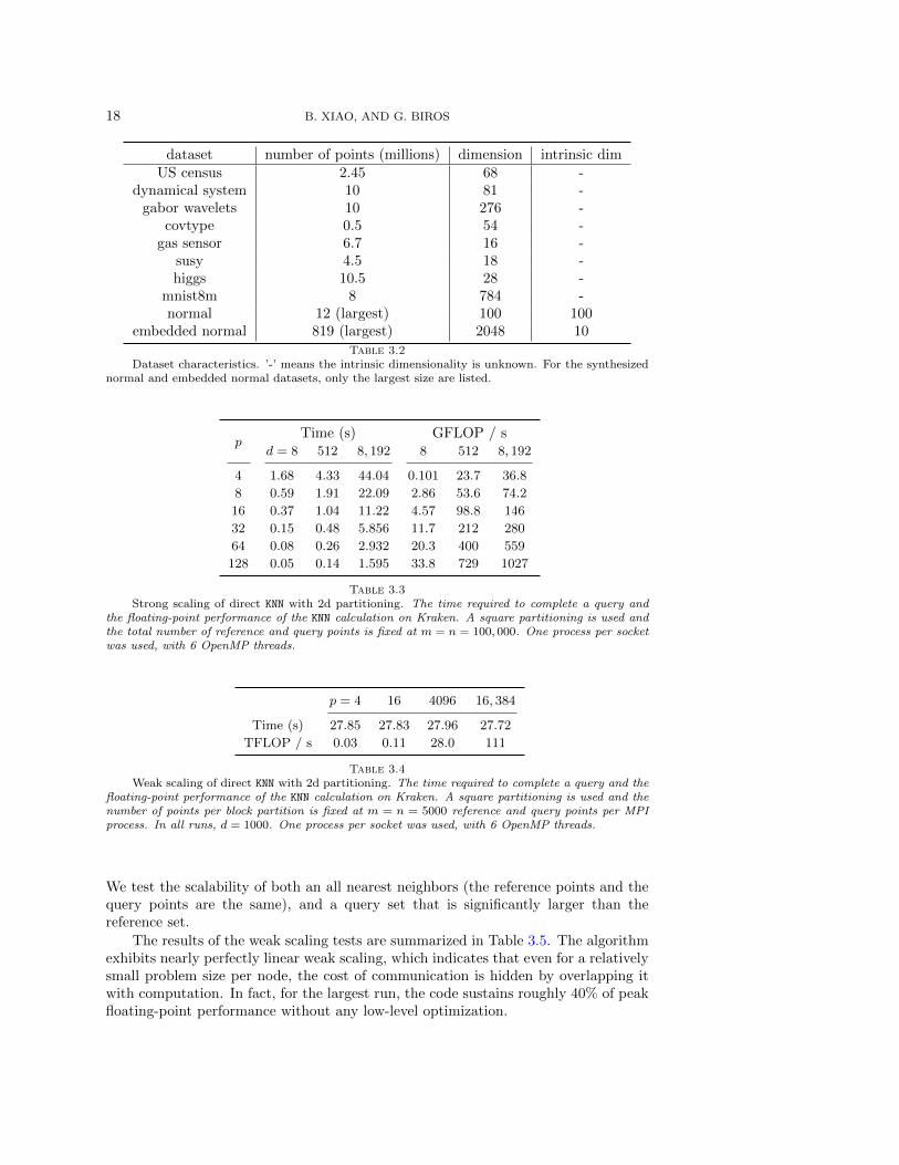
Datasets. We test the performance on several datasets, both synthetic and real.The synthetic datasets are points sampled from a normal distribution. Furthermore,we also generate an embedded normal dataset, which we first generate a d-dimensionalnormal data, then expand them into D-dimensional space by padding zeros and ro-tation. In this way, the dataset could have an intrinsic dimensionality d. In thefollowing, we denote the embedded normal data as ”d − D normal”. We also usesmall datasets to test and compare the exact tree search algorithms. The first oneis the US Census data from UCI Machine Learning Repository [22]. The second realdataset comes from the Gabor wavelet features of MRI cardiac images; The thirdone contains points from the phase space of a chaotic dynamical system. Finally,we test five large real datasets to show the accuracy and convergence of PKDT. Theyare ”covtype”, ”susy”, ”higgs”, ”gas sensor” from UCI Machine Learning Repository[22], and the frequently used hand written digit dataset ”mnist8m” [23]. Table 3.2summarize all the datasets used in this paper.
3.1. Brute force direct KNN performance. For the 2d partitioned direct k-NN, we evaluate performance by conducting strong-scaling tests on 48 to 768 cores(8 to 128 sockets) on Kraken. Our runs were performed with a fixed number of nodesoverall, m = n = 100, 000, and with three values of dimension, d = 8, 512, and 8192.The results in Table 3.3 show nearly perfect linear strong scaling, indicating thatthe communication and node interdependency caused by the k-reduction does notproduce a significant performance bottleneck. In Table 3.4, we demonstrate perfectlyflat weak scaling up to 16,384 MPI processes.
For the cyclic direct KNN, we evaluate performance by conducting weak-scalingtests on 12 to 12,288 cores (1 to 1024 nodes) on Kraken. In this experiment, we usea single MPI process per core and disable multi-threading within processes. Eventhough we do achieve good performance with hybrid parallelism, this decision wasmade to enable measuring the scalability to a larger number of independent processes.
18 B. XIAO, AND G. BIROS
dataset number of points (millions) dimension intrinsic dimUS census 2.45 68 -
dynamical system 10 81 -gabor wavelets 10 276 -
covtype 0.5 54 -gas sensor 6.7 16 -
susy 4.5 18 -higgs 10.5 28 -
mnist8m 8 784 -normal 12 (largest) 100 100
embedded normal 819 (largest) 2048 10
Table 3.2Dataset characteristics. ’-’ means the intrinsic dimensionality is unknown. For the synthesized
normal and embedded normal datasets, only the largest size are listed.
pTime (s) GFLOP / s
d = 8 512 8, 192 8 512 8, 192
4 1.68 4.33 44.04 0.101 23.7 36.8
8 0.59 1.91 22.09 2.86 53.6 74.2
16 0.37 1.04 11.22 4.57 98.8 146
32 0.15 0.48 5.856 11.7 212 280
64 0.08 0.26 2.932 20.3 400 559
128 0.05 0.14 1.595 33.8 729 1027
Table 3.3Strong scaling of direct KNN with 2d partitioning. The time required to complete a query and
the floating-point performance of the KNN calculation on Kraken. A square partitioning is used andthe total number of reference and query points is fixed at m = n = 100, 000. One process per socketwas used, with 6 OpenMP threads.
p = 4 16 4096 16, 384
Time (s) 27.85 27.83 27.96 27.72
TFLOP / s 0.03 0.11 28.0 111
Table 3.4Weak scaling of direct KNN with 2d partitioning. The time required to complete a query and the
floating-point performance of the KNN calculation on Kraken. A square partitioning is used and thenumber of points per block partition is fixed at m = n = 5000 reference and query points per MPIprocess. In all runs, d = 1000. One process per socket was used, with 6 OpenMP threads.
We test the scalability of both an all nearest neighbors (the reference points and thequery points are the same), and a query set that is significantly larger than thereference set.
The results of the weak scaling tests are summarized in Table 3.5. The algorithmexhibits nearly perfectly linear weak scaling, which indicates that even for a relativelysmall problem size per node, the cost of communication is hidden by overlapping itwith computation. In fact, for the largest run, the code sustains roughly 40% of peakfloating-point performance without any low-level optimization.

FAST KNN ALGORITHMS 19
pm = n = 1000 m = 100000, n = 100
Time (s) TFLOP/s Time (s) TFLOP/s
96 4.58 0.44 49.1 0.38
192 9.30 0.80 97.7 0.76
384 18.4 1.61 195 1.53
768 36.9 3.23 403 2.96
1,536 73.9 6.45 815 5.85
3,072 151 12.6 — —
6,144 303 25.2 — —
12,288 604 50.5 — —
Table 3.5Weak scaling of direct KNN with cyclic algorithm. The time required to complete a query and
the floating-point performance of the KNN calculation on Kraken. In all runs we used d = 100. Weuse one process per core. Here m and n indicate the number of points per MPI process.
3.2. KNN using PKDT. We have evaluated the KNN performance and scalability ofour tree-based approach on the Kraken platform using different datasets.
We first compared PKDTH and PKDTC . For the exact tree search, the most im-portant evaluation is how many points (or leaf nodes) a query should search. In theworst case a query visits all leaf nodes and no pruning takes place. In the best case,perfect pruning, every query visits only one leaf node. To measure the efficiency ofthe pruning, we define the pruning percentage as
pruner% =N − nrN −N/p
(3.1)
where N is the total number of query points among all processes; nr is the numberof query points on a single process r; p is the number of processes.
datasethyperplane partition (100%) clustering grouping (100%)min max avg min max avg
US census 45.90 99.98 89.92 32.87 99.87 63.83
dynamical system 97.76 99.97 98.99 0.6639 93.49 15.39
gabor wavelets 96.85 100.00 99.01 54.08 100.09 88.24
5d-100D normal 99.66 99.84 99.75 4.17 97.95 57.74
10d-100D normal 83.96 94.32 89.82 0 3.38 0.5456
Table 3.6Pruning effect of exact tree search on different datasets. The pruning is obtained using 5
different datasets. The US census run uses 9,100 reference points and 500 query points per process,and totally 256 processes. For the remaining four runs we use 10,000 reference points and 500query points per process, for a total of 1,024 MPI processes. The maximum, minimum and averagepruning percentage across all processes are reported.
Table 3.6 shows the pruning percentage of both PKDTH and PKDTC on 5 differentdatasets. Generally speaking, all those 5 datasets has lower intrinsic dimensionalitythan their ambient dimensions. As a result, even the dimension is high, there aresome pruning that could be obtained. We could find the clustering partition has less

20 B. XIAO, AND G. BIROS
pruning than the hyperplane partition on all the 5 datasets. On the other hand,unlike PKDTH which has a perfect load balance, it is very difficult to maintain theload balance for PKDTC . Since clustering is impossible to geneate clusters that allhave exact the same size, there is no guarantee then each kid has the same numberof reference points. All in all we prefer the hyperplane partition strategy, and in thefollowing scaling test, we only present the scalability of PKDTH .
p = 192 384 768 1536 3,072 6,144 12,288
5d
const. (s) 0.81 0.99 1.27 1.46 1.69 2.44 2.80
query (s) 3.82 4.25 5.10 5.81 13.07 18.92 28.42
% prune 98.86 99.40 99.68 99.83 99.91 99.95 99.97
10d
const. (s) 0.93 0.96 1.26 1.83 2.07 3.99 3.14
query (s) 37.61 55.92 81.57 115.72 162.11 267.27 379.75
% prune 75.04 82.41 87.99 91.96 94.74 96.54 97.56
Table 3.7Weak scaling of PKDTH for KNN (k = 2) using the normal distribution data. The time (in seconds)
required for tree construction and query on Kraken with a fixed number of points per process. 10,000reference points and 1000 query points per process were used for the 100-dimensional runs (pointsare sampled from a 5-dimensional normal distribution, and embedded into 100-dimensional space.)We use one MPI process per core.
We evaluate the weak scaling performance of PKDTH for KNN problem on 128 to24,576 cores (64 to 2048 nodes) on Kraken. In this experiment, we use a single MPIprocess per core and disable multi-threading within processes. Even through we doachieve good performance with hybrid parallelism, this decision was made to enablemeasuring the scalability to a larger number of independent processes. Performance issummarized in Table 3.7. We see that the construction time required to partition andredistribute the points grows very slowly as a function of problem size and processcount. However, for the query points, there is some overlap in the bounding regionsof the clusters, some number of query points will be replicated to multiple kids inthe tree traversal. Since we test the weak scaling using data sampled from a normaldistribution, as the process count increase, the density of data points becomes moreand more large. Thus, it is likely that at the very beginning, there is a big overlapnear the hyperplane. As going to deeper level, the overlap might be reduced. Thequery time increase quickly as the process count increases. This is mainly becauseas the process count increases, although the pruning percentage also is improved, thenumber of query points becomes larger on each leaf node, which means we shouldperform the direct nearest neighbor search kernel in a larges scale of data points. Forexample, when p = 12288, the maximum number of query points on a single leafnode is 417065, compared with 65951 for p = 192, which is 6.3 times larger. And toredistribute large amount of points also takes longer time. Generally speaking, thepruning degrades since the point density of the generated dataset increases rapidly asthe problem size is increased.
3.3. ANN using randomized PKDT. In our first experiment, we study the overallperformance of randomized PKDT in terms of accuracy, convergence, and wall-clocktime. We use five real datasets in Table 3.8 to solve the all nearest neighbors problem,i.e., the reference and query set are the same. Such runs are typical in learning tasksas part of cross-validation (e.g., to decide how many neighbors to use for a supervisedclassification problem).
FAST KNN ALGORITHMS 21
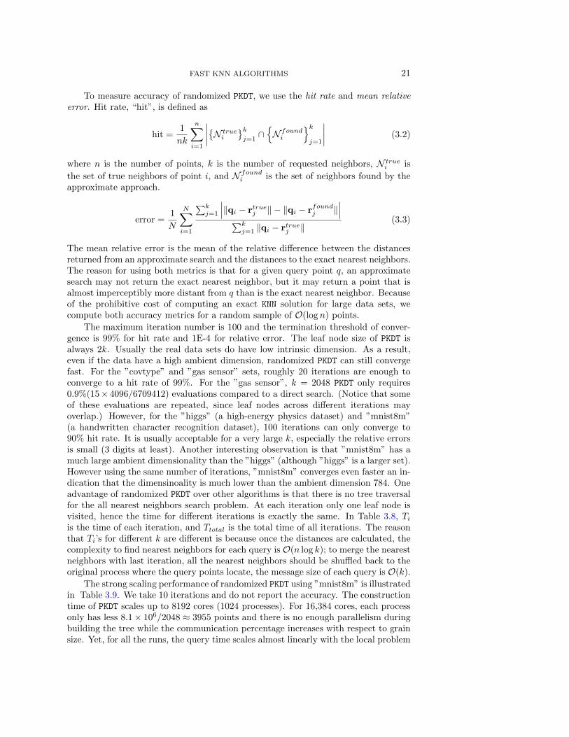
To measure accuracy of randomized PKDT, we use the hit rate and mean relativeerror. Hit rate, “hit”, is defined as
hit =1
nk
n∑i=1
∣∣∣∣{N truei
}kj=1∩{N foundi
}kj=1
∣∣∣∣ (3.2)
where n is the number of points, k is the number of requested neighbors, N truei is
the set of true neighbors of point i, and N foundi is the set of neighbors found by the
approximate approach.
error =1
N
N∑i=1
∑kj=1
∣∣∣‖qi − rtruej ‖ − ‖qi − rfoundj ‖∣∣∣∑k
j=1 ‖qi − rtruej ‖(3.3)
The mean relative error is the mean of the relative difference between the distancesreturned from an approximate search and the distances to the exact nearest neighbors.The reason for using both metrics is that for a given query point q, an approximatesearch may not return the exact nearest neighbor, but it may return a point that isalmost imperceptibly more distant from q than is the exact nearest neighbor. Becauseof the prohibitive cost of computing an exact KNN solution for large data sets, wecompute both accuracy metrics for a random sample of O(log n) points.
The maximum iteration number is 100 and the termination threshold of conver-gence is 99% for hit rate and 1E-4 for relative error. The leaf node size of PKDT isalways 2k. Usually the real data sets do have low intrinsic dimension. As a result,even if the data have a high ambient dimension, randomized PKDT can still convergefast. For the ”covtype” and ”gas sensor” sets, roughly 20 iterations are enough toconverge to a hit rate of 99%. For the ”gas sensor”, k = 2048 PKDT only requires0.9%(15× 4096/6709412) evaluations compared to a direct search. (Notice that someof these evaluations are repeated, since leaf nodes across different iterations mayoverlap.) However, for the ”higgs” (a high-energy physics dataset) and ”mnist8m”(a handwritten character recognition dataset), 100 iterations can only converge to90% hit rate. It is usually acceptable for a very large k, especially the relative errorsis small (3 digits at least). Another interesting observation is that ”mnist8m” has amuch large ambient dimensionality than the ”higgs” (although ”higgs” is a larger set).However using the same number of iterations, ”mnist8m” converges even faster an in-dication that the dimensinoality is much lower than the ambient dimension 784. Oneadvantage of randomized PKDT over other algorithms is that there is no tree traversalfor the all nearest neighbors search problem. At each iteration only one leaf node isvisited, hence the time for different iterations is exactly the same. In Table 3.8, Tiis the time of each iteration, and Ttotal is the total time of all iterations. The reasonthat Ti’s for different k are different is because once the distances are calculated, thecomplexity to find nearest neighbors for each query is O(n log k); to merge the nearestneighbors with last iteration, all the nearest neighbors should be shuffled back to theoriginal process where the query points locate, the message size of each query is O(k).
The strong scaling performance of randomized PKDT using ”mnist8m” is illustratedin Table 3.9. We take 10 iterations and do not report the accuracy. The constructiontime of PKDT scales up to 8192 cores (1024 processes). For 16,384 cores, each processonly has less 8.1× 10⁶/2048 ≈ 3955 points and there is no enough parallelism duringbuilding the tree while the communication percentage increases with respect to grainsize. Yet, for all the runs, the query time scales almost linearly with the local problem

22 B. XIAO, AND G. BIROS
dateset kNNname N d k iter hit rate error Ti Ttotal
covtype 500,000 54512 16 99.16% 6.4e-4 0.69 121024 16 99.01% 4.2e-4 1.37 242048 21 99.01% 1.7e-4 2.86 62
gas sensor 6,709,412 16512 21 99.11% 5.4e-4 8.12 1801024 18 99.05% 6.1e-4 16.67 3122048 15 99.04% 7.2e-4 33.36 531
susy 4,500,000 18512 60 99.15% 4.6e-4 5.27 3201024 55 99.01% 4.8e-4 10.48 5842048 51 99.03% 4.8e-4 21.62 1120
higgs 10,500,000 28512 100 80.47% 1.0e-2 12.59 12641024 100 83.90% 7.8e-3 24.98 25182048 100 88.08% 5.3e-3 50.32 5054
mnist8m 8,100,000 784512 100 86.37% 6.4e-3 18.93 19041024 100 88.92% 4.8e-3 29.92 29992048 100 91.21% 3.4e-3 53.63 5413
Table 3.8Accuracy and time on several large real datasets of randomized PKDT. All the experiments are
run on Maverick using 32 nodes, one MPI process per socket. ’Ti’ is the time for each iteration,’Ttotal’ is the total time spent. The maximum iteration number is set to be 100, and once the hit ratetouches 99%, the iteration will terminate automatically. Also in all experiments, we construct thetree so that each leaf node has no more than 2k points, where k is the number of nearest neighbors.Notice that this gives an indication of the overall distance evaluations. For example for the k = 512”mnist8m” run, we take 100 PKDT iterations, which in turn means that we perform 102,400 distanceevaluations per query point or 1.2% of evaluations required in a direct evaluation. For the k = 2046this number increases to 5%. For the ”gas sensor” dataset, we see that in all cases less than 1%evaluations end up giving almost exact solutions, and indication that the intrinsic dimensionality isreally small.
size O(nd/p).
cores 1,024 2,048 4,096 8,192 16,384
MNIST8Mconstruction 51.75 31.67 18.99 12.11 18.55
query 542.71 257.48 132.70 71.67 48.11speedup 1 2.06 3.92 7.10 8.92
Table 3.9Strong Scaling of PKDT on Maverick: Strong scaling of 10 iterations of PKDT on Maverick for the
”mnist8m” dataset. In this run, k is 2048, the maximum leaf node size is then 4096. ’construction’stands for tree construction time of the tree in total 10 iterations, and ’query’ is the total queryingtime. The point-wise data exchange is applied in these runs.
Next we study the weak scaling performance of randomized PKDT. First of all, wewant to compare three difference data exchange mechanism discussed in §2.3.2. Forthe purpose of extensively comparison, we tested only the tree construction part onthree different machines: Lonestar, Kraken and Jaguar. We use the metric millionsof cycles / point / core to compare across platforms, i.e., the number of clock cyclesthat would be needed to perform the query for each point using only a single core.
On Lonestar (Table 3.10), the lower bandwidth of interconnect combined withits less-tuned MPI stack clearly shows the differences in the scalability of the threemethods. the whole tree exchange performs well at small scales, but point-wise data

FAST KNN ALGORITHMS 23
exchange shows the best overall scalability. Weak-scaling results for point-wise dataexchange and the whole tree exchange on Kraken are presented in Table 3.11. Heretoo, the whole tree exchange performs well at small p but does not scale well as weincrease the processes; however, point-wise exchange maintains very good efficiencyup to 96K cores. Table 3.12 presents weak-scaling results for all three data exchangeon Jaguar. On Jaguar, the differences between the three construction algorithms areless marked, with the exception of the fact that whole tree exchange also fails to scaleto large p. Overall speaking, the whole tree exchange provides the best performanceat small p but does not scale well at large p. Point-wise exchange exhibits slightlybetter performance and scalability than all-to-all exchange. It is not currently clearwhy point-wise exchange fails to maintain the same level of parallel efficiency onJaguar that it exhibits on Kraken at comparable core counts. Further investigationis necessary to explain this behavior.
Tree: Lonestar weak scalingcores 192 384 768 1,536 3,072 6,144
all-to-all exchangecycles 10.7 17.8 25.3 39.1 58.0 88.5effic 100% 60% 42% 27% 18% 12%
point-wise exchangecycles 6.9 8.4 9.8 11.3 13.0 15.2effic 100% 83% 71% 62% 54% 46%
whole tree exchangecycles 5.7 7.3 8.4 10.2 12.6 17.6effic 100% 78% 69% 56% 45% 32%
Table 3.10Weak-scaling of Tree Construction on Lonestar. This table shows the scalability of the three tree
construction variants on Lonestar in terms of millions of cycles per point per core and the efficiencyrelative to the 192-core run. We use one process per socket with 6 OpenMP threads. We use 10Kpoints per process in 2,048 dimensions.
Tree: Kraken weak scalingcores 1,536 3,072 6,144 12,288 24,576 49,152 98,304
point-wise exchangecycles 18.0 17.9 21.2 25.8 30.1 36.0 43.1effic 100% 100% 85% 70% 60% 50% 42%
whole tree exchangecycles 14.0 12.5 20.7 31.7 59.3 - -effic 100% 112% 68% 44% 24% - -
Table 3.11Weak-scaling of Tree Construction on Kraken. This table shows the scalability of point-wise data
exchange and the whole tree exchange on Kraken in terms of millions of cycles per point per core.The efficiency relative to the 1.5K core run. We use 10K points per process in 2,048 dimensions.
Finally, we illustrate the weak scaling performance of the randomized PKDT onStampede and Jaguar. The data exchange method is the point-wise exchange for allruns. On stampede, we use 1024 normal distribution data; each process has 50,000points; one process per socket with 8 threads. We test k = 2048 in this run. InFigure 3.1, it is clear that the query part is the most expensive portion since selecting

24 B. XIAO, AND G. BIROS
Tree: Jaguar weak scalingcores 2,048 4,096 8,192 16,384 32,768 65,536 131,072
all-to-all exchangecycles 11.1 16.4 20.3 27.3 33.5 46.1 51.1effic 100% 68% 55% 41% 33% 27% 22%
point-wise exchangecycles 9.8 12.5 15.8 22.9 32.4 38.8 49.8effic 100% 78% 62% 43% 30% 25% 20%
whole tree exchangecycles 5.3 8.1 10.7 25.5 34.2 132.3 -effic 100% 66% 50% 21% 16% 4% -
Table 3.12Weak-scaling of Tree Construction on Jaguar. This table shows the scalability of the three tree
construction variants on Jaguar in terms of millions of cycles per point per core and the efficiencyrelative to the 2048-core run. We use one process per socket with 8 OpenMP threads. We use 10Kpoints per process in 2,048 dimensions.
k neighbors requires maintaining a maximum heap of size k as well as merging kneighbors from the last iteration for each point. The construction part is linear withrespect to the number of processes, which is consistent with the analysis in §2.3.2.The query part is almost constant because the local problem size is the same due tothe load balanced data exchange mechanism. Overall if k is relative large, PKDT canget nearly constant weak scaling performance. For the small k case, we test the allnearest neighbors case on Jaguar using 2048 dimensional normal data; each processhas 50,000 points; one process per socket with 8 threads. In the case of Figure 3.2k = 2, the tree construction dominates the overall running time. Similarly, the querytime is nearly constant but the construction time scales with respect to the numberof processes.
We used the normalized cycles / points / core statistic to compare performancesacross different systems. For weak scaling, increasing numbers indicate communica-tion overheads and load imbalance. Notice that algorithmically we show that thebest-case complexity estimates include terms that grow with powers of log p, linearlyin p, or with factors that depend on log n that inherently limit the attainable efficien-cies.
This is the first time that nearest neighbors solver has been scaled to this extentand a first attempt to characterize the parallel scalability of state-of-the-art approxi-mate nearest neighbors methods in leadership architectures. However, there are somegeneral conclusions that can be drawn. During the tree construction, the clear loserin three different data exchange technique is the whole tree exchange, but again thereare regimes in which it performs well (small number of core counts). The interplaybetween latency, bandwidth, points per leaf node size suggests significant opportuni-ties for performance tuning and optimization depending on the machine architecture,the dataset and its dimensionality.
3.4. Comparison with existing software packages. As we mentioned, nosoftware offers the capabilities of our library. But just do indicate that even in thesingle node case, we outperform existing codes, we discuss a few examples. The firstpackage we discuss is MLPACK, which is only supports exact searches, but does nothave distributed memory parallelism. The larger dataset reported in [8] is has 1M
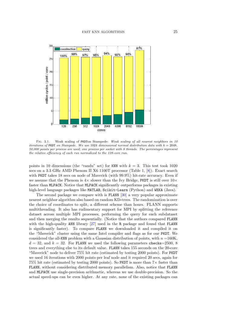
FAST KNN ALGORITHMS 25
Fig. 3.1. Weak scaling of PKDTon Stampede: Weak scaling of all nearest neighbors in 10iterations of PKDT on Stampede. We use 1024 dimensional normal distribution data with k = 2048.50,000 points per process are used; one process per socket with 8 threads. The percentages representthe relative efficiency of each run normalized to the 128-core run.
points in 10 dimensions (the “randu” set) for KNN with k = 3. This test took 1020secs on a 3.3 GHz AMD Phenom II X6 1100T processor (Table 1, [8]). Exact searchwith PKDT takes 18 secs on node of Maverick (with 99.9%) hit-rate accuracy. Even ifwe assume that the Phenom is 4× slower than the Ivy Bridge, PKDT is still over 10×faster than MLPACK. Notice that MLPACK significantly outperforms packages in existinghigh-level language packages like MATLAB, Scikit-Learn (Python) and WEKA (Java).
The second package we compare with is FLANN [30] a very popular approximatenearest neighbor algorithm also based on random KD-trees. The randomization is overthe choice of coordinates to split, a different scheme than hours. FLANN supportsmultithreading. It also has rudimentary support for MPI by splitting the referencedataset across multiple MPI processes, performing the query for each subdatasetand then merging the results sequentially. (Notice that the authors compared FLANN
with the high-quality ANN library [27] used in the R package and found that FLANN
is significantly faster). To compare FLANN we downloaded it and compiled it onthe “Maverick” cluster using the same Intel compiler and flags as for our PKDT. Weconsidered the all-KNN problem with a Gaussian distribution of points, with n =160K,d = 32, and k = 32. For FLANN we used the following parameters checks=2500, 8trees and everything else to its default value. FLANN takes 155 seconds on the 20-core“Maverick” node to deliver 75% hit rate (estimated by testing 2000 points). For PKDTwe used 16 iterations with 2000 points per leaf node and it required 20 secs, again for75% hit rate (estimated by testing 2000 points). So PKDT is more than 7× faster thanFLANN, without considering distributed memory parallelism. Also, notice that FLANN
and MLPACK use single-precision arithmetic, whereas we use double-precision. So theactual speed-ups can be even higher. At any rate, none of the existing packages can

26 B. XIAO, AND G. BIROS
Fig. 3.2. Weak scaling of PKDTon Jaguar: Weak scaling of all nearest neighbors in 8 iterationsof PKDT on Jaguar. We use 2048 dimensional normal distribution data with k = 2048. 50,000 pointsper process are used; one process per socket with 8 threads. The percentages represent the relativeefficiency of each run normalized to the 2,048-core run.
handle the large datasets one which we test PKDT.

FAST KNN ALGORITHMS 27
4. Conclusion. We presented a set of algorithms for the parallel tree construc-tion for points in high-dimensions, for exact nearest neighbor searches, and for ap-proximate nearest-neighbor searches using greedy search on randomized KD-trees. Wereported the accuracy and scalability of the scheme for synthetic and non-syntheticdatasets across different clusters and problem sizes and we demonstrated unprece-dented scalability. As mentioned in the introduction the software is athttp://padas.ices.utexas.edu/matheme.
There are several things we did not have space to discuss. For example in [19]the idea of “supercharging” is discussed in which the greedy search is augmented bysearch on the nearest-neighbor graph. We implemented this in PKDT but we found,consistently, that in the distributed memory setting the procedure is not effectivedue to unpredictable memory loads and communication overheads: simply takingmore iterations is faster and more robust. Also, we have implemented a parallelLSH algorithm. In a nutshell, similar good performance (in terms of accuracy andscalability) can be obtain with the LSH algorithm, however it requires significantparameter tuning for each dataset, whereas PKDT offers similar performance with notuning parameters. The discussion of the comparison will be reported elsewhere.
Appendix A. Point Grouping Using kmeans Clustering with Random-ized Seeds. In this section, we outline the point-grouping mechanism, the kmeansclustering. We use a standard kmeans clustering algorithm with the seeding intro-duced in Ostrovsky et al. [32]. Its main feature is that it reduces the number ofiterations required to converge the kmeans algorithm and most importantly, removesthe need for multiple invocation of kmeans with different seeds. For well-clusterablecases (e.g., mixtures of well-separated Gaussians), the new clustering can be ordersof magnitude faster than uniformly randomly selecting seeds among the input pointsbecause it eliminates the need for repeated seed selection.
Parallelizing kmeans is straightforward [11]. Algorithm 11 describes the scheme.It is easy to see that the complexity per iteration is O(kd(np + log p)), where k is the
Algorithm 11 kMeans(r, c, n, k)
1: for j = 1 · · ·n do2: For each point rj , assign cluster membership by finding the closest centers ci3: ci =
∑rj , rj ∈ cluster i (Vi), |Vi| = ni
4: ni = Allreduce(ni)5: ci = Allreduce(ci)6: ci = ci/ni7: end for
number of clusters, n is the number of points, and p is the number of processors.
A.1. Seeding. To reduce the iterations of standard kmeans and obtain highquality clusters, seeds can be carefully selected. A choice of the initial centroids(seeding) with provable quality guarantees (under a quantitative assumption of clus-terability) is discussed in [32]. Once the seeds have been computed, the ball-kmeansor the standard kmeans iteration can be used. The algorithm in [32] is based on theobservation that k initial centroids that are far away from each other will belong to kdifferent clusters. To find these points, we first oversample on probabilities based onthe interpoint distances and then we eliminate bad seeds.
The oversampling step is summarized by Algorithm 12. First, we sample two

28 B. XIAO, AND G. BIROS
initial seeds (denote as s1 and s2) according to probabilities
p1j =
(d2(rj , r)n+
∑j d
2(rj , r))
(2n∑j d
2(rj , r)) (A.1)
p2j =d2 (rj , s1)(∑
j d2(rj , r) + nd2(r, s1)
) (A.2)
where n is the number of points, r is the global mean of all points rj , s1 is the firstselected seed, and d(·, ·) is the distance between two points.
Then, for the remaining points, the sampling probability is given by
pj =d2(rj , s
j∗)∑
rjd2(rj , s
j∗)
(A.3)
where d(rj , sj∗) is the distance between point rj and its nearest seed sj∗, which has
already been chosen. Finally, a randomly sampled point based on the probabilityfrom the unchosen set is used until a new seed is added. We repeat these steps untilwe have chosen k seeds.
Algorithm 12 addSeeds(r, s, k)
1: if isempty(s) then2: sample the first two seeds s1 and s23: end if4: if |s| ≥ k then return5: d(rj , s
j∗) = minsi d(si, rj)
6: compute sampling probabilities p = {pj} according to Eq. A.37: s′ = random sample(r/{s}, p)8: s← s ∪ s′9: addSeeds(r/{s}, s, k)
After oversampling k′ seeds where k′ > k, We eliminate these seeds one by one toexclude those which generate bad clustering quality, until finally we have k centers.The seed elimination step is described in Algorithm 13. In more detail, we evaluatethe clustering quality of k′ − 1 seeds {si}k
′
i=1\sj for each sj , then delete the one withthe lowest quality. The clustering quality is measured by the kmeans loss L,
Lk(X) =1
|X|
k∑i=1
∑x∈Vi
‖x− si‖2 (A.4)
where Vi is the Voronoi set of seed si. If the data is ε-separated, which implies
Lk(X)/Lk−1(X) ≤ ε2, [32] suggests oversampling k′ = 2k1−5√ε
+ 2 log(2/√ε)
(1−5√ε)2
points is
sufficient to obtain good results. In practice, without any prior knowledge about theε, it is possible to estimate it by using a small subset of the input data.
k-Means seeding performance. We compare the performance of two typesof seeding approaches for kmeans. The first one is the standard uniformly randomly

FAST KNN ALGORITHMS 29
Algorithm 13 EliminateSeeds(r, s, k)
1: if |s| ≤ k then return2: for i = 1 : |s| do3: ni = |Vi| for si4: s(i) ← s\si5: compute the kmeans loss L(i) of s(i)
6: Ti = niL(i)
7: end for8: s∗ = mins Ti9: s← s\s∗
10: for i = 1 : |s| do11: find Vi for each si12: si ← mean(Vi)13: end for14: EliminateSeeds(r, s, k)
selection of seeds among the input points; the other is the Ostrovsky seeding.Experiments run on the synthetic data, a mixture of eight Gaussians with unit
variance. Each center of these Gaussians is located on a vertex of a hypercube. Eachrun was repeated 100 times. Clustering quality is measured by the loss functionEqn. A.4 and the variance ratio V
V(X) = max
∑ki=1 pi‖ci − c‖2∑k
i=1 pi1|Vi|∑x∈Vi‖x− ci‖2
, (A.5)
where pi = ‖Vi‖‖X‖ and c is the center of the whole dataset X. The higher the variance
ratio, the better clustering quality is.
D k seeding L(X) V(X) iters accuracy
3
4random 4. 11±0.061 1.15±0.032 11.28±3.64 45.81%±0.88%
Ostrovsky 4.10±0.046 1.16±0.024 11.01±4.33 45.61%±0.63%
8random 1.95±0.160 3.57±0.330 11.03±3.75 87.12%±5.65%
Ostrovsky 1.97±0.171 3.51±0.361 8.02±3.57 86.30%±6.01%
6
4random 11.20±0.421 1.60±0.083 7.91±2.85 49.91%±0.06%
Ostrovsky 11.09±0.008 1.62±0.002 6.41±2.69 49.93%±0.04%
8random 3.55±1.216 8.34±3.528 7.44±2.29 91.25%±7.13%
Ostrovsky 2.16±0.368 12.69±1.203 3.17±0.88 99.50%±2.16%
Table A.1Clustering Quality: The clustering quality is measured by the kmeans loss, variance ratio,
number of kmeans iterations (iters), and the clustering accuracy (accuracy). We use a mixture of8 Gaussians. Here D is the distance between each pair of Gaussian centers. k indicates the numberof target clusters (the best k is eight).
When the length of the hypercube edges is 6, the Gaussians are relatively wellseparated, it is clear that the Ostrovsky seeds results in a better clustering thanrandom selected seeds. First, the loss function and variance ratio indicate betterquality. Second, the standard deviations of these measures are much smaller than

30 B. XIAO, AND G. BIROS
those of random seeds, which implies the Ostrovsky seeds are more stable and canbe expected to always produce good clustering results. Third, the Ostrovsky seedsrequire less iterations to converge. We also test the case of edge length 3. In this case,there is no significant difference between two types of seedings. Generally speaking,only the Ostrovsky seeding can be ”safely” used without need for repeated seeding,which is expensive as it requires collective communication. On the other side, theOstrovsky seeds could also be a good clusterability heuristic. The loss function andthe variance ratio will vary slightly when k is close to the number of data’s intrinsicgroups. In Figure A.1, it is clear that the slope of the Ostrovsky seeding curve changessharply when k = 8, which is the number of Gaussians we used. As a counterpart, itis less pronounced using uniformly random selected seeds.
Fig. A.1. Clusterability: The change in the value of the loss and the variance ratio is anindication for the intrinsic number of clusters existing in the data. The blue lines stand for thekmeans loss and the green lines stand for the variance ratio. The solid lines are the Ostrovsky seeds,the dashed lines indicate random seeds. The x-axis is the number of clusters.
Appendix B. Clustering Tree. We briefly outline the construction of theclustering tree. The node splitting algorithm works as follows:
Let T be a tree node, XT be all the points assigned in T , lT be the level of thenode T in the tree, and sT be the size of node T ’s communicator. Let i be a clusterof points with centroid ci and radius Ri, Bc,R be a closed ball in Rd centered at c withradius R, Ci be the tree node that owns group i, and Nc be the number of clusterscreated in each split. Algorithm 14 describes the node-splitting procedure.
As outlined in Algorithm 14, we use a distributed top-down algorithm to constructthe tree and, at each level, split a node to two children, each of which contain one ormore groups of points. For assigning points to groups, we use our distributed kmeansroutine. Except that, the remaining point repartition and communicator splittingprocedures are similar to the PKDT.
Finally we sketch the complexity of the tree construction algorithm, assuming auniform tree. Let l be the level of a node. Computing the clusters takes O(d(nl/pl +log pl)) time, where nl = n/2l are the points per node at the lth level and pl = p/2l
are the number of processors per node at the lth level. Furthermore, the collective to

FAST KNN ALGORITHMS 31
Algorithm 14 nodeSplit(T )
1: if lT ==maxLevel || |XT | < minNumofPoints then2: return;3: else4: addSeeds(XT , seeds,Nc)5: eliminateSeeds(XT , seeds,Nc)6: centroids = kMeans(XT , seeds,Nc)7: for each point x ∈ XT do8: Assign x to cluster i such that d(x, ci) is minimized9: end for
10: Assign clusters to children such that each child has roughly the same amountof points
11: Assign processes for each child Ci12: Split T ’s communicator, creating a new communicator for each Ci13: Distribute points in each cluster i to processes in Ci14: nodeSplit(Clocal)15: end if
redistribute points within the node takes O(nl
p2lpl) time (ignoring latency). From these
observations we can see that the overall complexity of the tree construction (assuminga uniform tree) is O(dnp log2 p).
Appendix C. Distributed Select. To find the median value of an unorderedarray, we apply a select operation. Select(k) finds the kth smallest value in an array.For the median we use Select(n/2), where n is the total number of input elements.Algorithm 15 describes our distributed-memory select function. A more sophisticated
Algorithm 15 ParSelect(arr, k)
1: N = AllReduce(arr.size())2: choose a pivot point x from arr at random3: arr less = [] arr great = []4: for each point i in input array arr do5: if arr[i] > x then6: arr less.insert( arr[i] )7: else8: arr great.insert( arr[i] )9: end if
10: end for11: Nl = AllReduce(arr less.size())12: Ng = AllReduce(arr great.size())13: if N == 1 ‖ Nl == k ‖ Nl == N ‖ Ng == N then14: return x15: else if Nl > k then16: ParSelect(arr less, k)17: else18: ParSelect(arr great, k −Nl)19: end if
algorithm and more discussion can be also found in [43].

32 B. XIAO, AND G. BIROS
REFERENCES
[1] Mathematics of analysis of petascale data. Technical report, DOE Office of Science, 2008.[2] Dror Aiger, Efi Kokiopoulou, and Ehud Rivlin. Random grids: Fast approximate nearest
neighbors and range searching for image search. In Computer Vision (ICCV), 2013 IEEEInternational Conference on, pages 3471–3478. IEEE, 2013.
[3] I. Al-Furajh, S. Aluru, S. Goil, and S. Ranka. Parallel construction of multidimensional binarysearch trees. Parallel and Distributed Systems, IEEE Transactions on, 11(2):136–148,2000.
[4] A. Andoni and P. Indyk. E2LSH 0.1 User manual, 2005. http://www.mit.edu/~andoni/LSH.[5] A. Andoni and P. Indyk. Near-Optimal Hashing Algorithms for Approximate Nearest Neighbor
in High Dimensions. COMMUNICATIONS OF THE ACM, 51(1):117, 2008.[6] Alina Beygelzimer, Sham Kakade, and John Langford. Cover trees for nearest neighbor. In
ICML, pages 97–104, 2006.[7] P. Ciaccia, M. Patella, and P. Zezula. M-tree an efficient access method for similarity search
in metric spaces. Proceedings of the 23rd VLDB Conference, pages 426–435, 1997.[8] Ryan R. Curtin, James R. Cline, Neil P. Slagle, William B. March, P. Ram, Nishant A. Mehta,
and Alexander G. Gray. MLPACK: A scalable C++ machine learning library. Journal ofMachine Learning Research, 14:801–805, 2013.
[9] S. Dasgupta and Y. Freund. Random projection trees and low dimensional manifolds. InProceedings of the 40th annual ACM symposium on Theory of computing, pages 537–546.ACM, 2008.
[10] Karen D. Devine, Erik G. Boman, and George Karypis. Partitioning and load balancing foremerging parallel applications and architectures. In M. Heroux, A. Raghavan, and H. Si-mon, editors, Frontiers of Scientific Computing. SIAM, Philadelphia, 2006.
[11] I. Dhillon and D. Modha. A data-clustering algorithm on distributed memory multiprocessors.Large-Scale Parallel Data Mining, pages 802–802, 2000.
[12] J. H. Freidman, J. L. Bentley, and R. A. Finkel. An algorithm for finding best matches inlogarithmic expected time. ACM Trans. Math. Softw., 3:209–226, 1977.
[13] J. Friedman, T. Hastie, and R. Tibshirani. The elements of statistical learning, volume 1.Springer Series in Statistics, 2001.
[14] K. Fukunaga and P. M. Narendra. A brach and bound algorithm for computing k-nearestneighbors. IEEE Trans. Comput., 24:750–753, 1975.
[15] B. Ganapathysubramanian and N. Zabaras. A non-linear dimension reduction methodologyfor generating data-driven stochastic input models. Journal of Computational Physics,227(13):6612–6637, 2008.
[16] V. Garcia, E. Debreuve, and M. Barlaud. Fast k nearest neighbor search using GPU. 2008.[17] Fabian Gieseke, Justin Heinermann, Cosmin Oancea, and Christian Igel. Buffer k-d trees: Pro-
cessing massive nearest neighbor queries on GPUs. In Proceedings of the 31st InternationalConference on Machine Learning (ICML), volume 32 of JMLR W&CP, pages 172–180.JMLR.org, 2014.
[18] A.G. Gray and A.W. Moore. N-Body’problems in statistical learning. Advances in neuralinformation processing systems, pages 521–527, 2001.
[19] P.W. Jones, A. Osipov, and V. Rokhlin. Randomized approximate nearest neighbors algorithm.Proceedings of the National Academy of Sciences, 108(38):15679–15686, 2011.
[20] D. Karger and M. Ruhl. Finding nearest neighbors in growth restricted metrics. Proceeding ofSTOC, 2002.
[21] I. Lashuk, A. Chandramowlishwaran, T-A. Nguyen H. Langston, R. Sampath, A. Shringarpure,R. Vuduc, D. Zorin L. Ying, and G. Biros. A massively parallel adaptive fast-multipolemethod on heterogeneous architectures. In SC ’09: Proceedings of the 2009 ACM/IEEEconference on Supercomputing, pages 1–12, Piscataway, NJ, USA, 2009. IEEE Press.
[22] M. Lichman. UCI machine learning repository, 2013.[23] Gaelle Loosli, Stephane Canu, and Leon Bottou. Training invariant support vector machines
using selective sampling. In Large Scale Kernel Machines, 2007.[24] William B. March, Bo Xiao, and George Biros. ASKIT: Approximate skeletonization kernel-
independent treecode in high dimensions. SIAM Journal on Scientific Computing,37(2):1089–1110, 2015.
[25] William B. March, Bo Xiao, Chenhan Yu, and George Biros. An algebraic parallel treecodein arbitrary dimensions. In Proceedings of IPDPS 2015, 29th IEEE International Paralleland Distributed Computing Symposium, Hyderabad, India, May 2015. acceptance rate107/495 (21.8%).
[26] G.L. Miller, S.H. Teng, W. Thurston, and S.A. Vavasis. Separators for sphere-packings and

FAST KNN ALGORITHMS 33
nearest neighbor graphs. Journal of the ACM (JACM), 44(1):1–29, 1997.[27] D.M. Mount and S. Arya. Ann: A library for approximate nearest neighbor searching. In CGC
2nd Annual Fall Workshop on Computational Geometry, 1997. www.cs.umd.edu/~mount/
ANN/.[28] Marius Muja and David G. Lowe. Fast approximate nearest neighbors with automatic algorithm
configuration. In International Conference on Computer Vision Theory and ApplicationVISSAPP’09), pages 331–340. INSTICC Press, 2009. www.cs.ubc.ca/~mariusm/index.
php/FLANN/FLANN.[29] Marius Muja and David G. Lowe. Fast approximate nearest neighbors with automatic algorithm
configuration. In In VISAPP International Conference on Computer Vision Theory andApplications, pages 331–340, 2009.
[30] Marius Muja and David G Lowe. Scalable nearest neighbor algorithms for high dimensionaldata. Pattern Analysis and Machine Intelligence, IEEE Transactions on, 36(11):2227–2240, 2014.
[31] S. M. Omohundro. Efficient algorithms with neural network behavior. J. of Complex Systems,2:273–347, 1987.
[32] R. Ostrovsky, Y. Rabani, L.J. Schulman, and C. Swamy. The effectiveness of Lloyd-typemethods for the k-means problem. In Foundations of Computer Science, 2006. FOCS’06.47th Annual IEEE Symposium on, pages 165–176. IEEE, 2006.
[33] J. Pan, C. Lauterbach, and D. Manocha. Efficient nearest-neighbor computation for GPU-basedmotion planning. In Intelligent Robots and Systems (IROS), 2010 IEEE/RSJ InternationalConference on, pages 2243–2248. IEEE, 2010.
[34] Jia Pan and Dinesh Manocha. Fast gpu-based locality sensitive hashing for k-nearest neighborcomputation. ACM SIGSPATIAL GIS, pages 211–220, 2011.
[35] Krauthgamer R. and J. Lee. Navigating nets: Simple algorithms for proximity search. Pro-ceedings of the 15th Annual Symposium on Discrete Algorithms (SODA), pages 791–801,2004.
[36] A. Rahimian, I. Lashuk, S.K. Veerapaneni, A. Chandramowlishwaran, D. Malhotra, L. Moon,R. Sampath, A. Shringarpure, J. Vetter, R. Vuduc, D. Zorin, and G. Biros. Petascaledirect numerical simulation of blood flow on 200k cores and heterogeneous architectures.In SC ’10: Proceedings of the 2010 ACM/IEEE conference on Supercomputing, pages 1–12,Piscataway, NJ, USA, 2010. IEEE Press.
[37] P. Ram, D. Lee, W. March, and A. Gray. Linear-time algorithms for pairwise statisticalproblems. Advances in Neural Information Processing Systems, 23, 2009.
[38] Carl Edward Rasmussen and Christopher Williams. Gaussian Processes for Machine Learning.MIT Press, 2006.
[39] S.T. Roweis and L.K. Saul. Nonlinear dimensionality reduction by locally linear embedding.Science, 290(5500):2323–2326, 2000.
[40] H. Samet. Foundations of multidimensional and metric data structures. Morgan Kaufmann,2006.
[41] Bernhard Scholkopf and Alexander J Smola. Learning with kernels: support vector machines,regularization, optimization, and beyond. MIT press, 2002.
[42] N. Sismanis, N. Pitsianis, and X. Sun. Parallel search of k-nearest neighbors with synchronousoperations. IEEE Conference on High Performance Extreme Computing, pages 1–6, 2012.
[43] Hari Sundar, Dhairya Malhotra, and George Biros. HykSort: A new variant of hypercubequicksort on distributed memory architectures. In ICS’13: Proceedings of the InternationalConference on Supercomputing, 2013, 2013.
[44] J. Tenenbaum, V. Silva, and J. Langford. A global geometric framework for nonlinear dimen-sionality reduction. Science, 290(5500):2319–2323, 2000.
[45] A. Torralba, R. Fergus, and W.T. Freeman. 80 million tiny images: A large data set fornonparametric object and scene recognition. IEEE Transactions on Pattern Analysis andMachine Intelligence, pages 1958–1970, 2008.
[46] J. K. Uhlmann. Satisfying general proximity/similarity queries with metric trees. InformationProcessing Letter, 40:175–179, 1991.
[47] R. Weber, H.J. Schek, and S. Blott. A quantitative analysis and performance study forsimilarity-search methods in high-dimensional spaces. In Proceedings of the InternationalConference on Very Large Data Bases, pages 194–205. IEEE, 1998.