Paradise Lost and Regained: Transportation Innovation...

JOURNAL OF URBAN ECONOMJCS 13,67-89 (1983)

Paradise Lost and Regained: Transportation Innovation,

Income, and Residential Location

STEPHEN F.LERoY ANDJON SONSTELIE

Department of Economics, University of California, Santa Barbara, California 93106

Received April 15, 198 I ; revised September 8, 198 1

1. INTRODUCTION

It was long characteristic of American cities that the rich lived on the edges while the poor lived in the centers. In the 197Os, however, that residential pattern began to change as rich households moved into many city centers, displacing the poor. In this paper, we offer au account both of why the earlier pattern prevailed until the 1970s and of why it is changing now.

The key to our explanation is the altered role of the car as a means of commuting to work. When the car first became practical for commuting it gave the rich access to cheaper suburban land than was available to the poor. Accordingly, the rich lived in the suburbs and the poor in the city centers. The relative cost of commuting by car has fallen, however, and now almost everyone can afford it. The poor, therefore, now have access to suburban locations and, thus, the comparative advantage the rich once had in those locations has been eroded. Consequently, the rich are beginning to return to the city centers.

Our explanation is based on a simple extension of the model developed by Alonso [l], Muth [15], and others. In the Alonso-Muth model employment is concentrated in a central business district (CBD), and workers commute to that CBD from a residential area surrounding it. Because the cost of commuting increases with the length of the commute, the unit rent of housing must fall with distance from the CBD. Households of different incomes will base their choice of where to live upon two opposing sources of benefit. First, since the rich use more housing than the poor, they benefit by living farther from the CBD where the rent of housing is lower. Second, however, the rich value their time more highly than the poor, so they benefit from living nearer the center of the city, where commuting times are shorter.

67

0094-l 190/83/010067-23$03.00/O Copyright 0 1983 by Academic Press, Inc.

All rights of reproduction in any form reserved.

68 LEROY AND SONSTELIE

In the Alonso-Muth model, it turns out, the former effect dominates and the rich live farther from the CBD than the poor if and only if the income elasticity of housing demand exceeds the income elasticity of marginal commuting cost. Where the theory predicts that the rich and poor will live thus depends on which of these two magnitudes is greater. The income elasticity of marginal communting cost is less than one, since the material cost of commuting does not vary proportionally with income, while the value of time may be assumed to do so. The income elasticity of housing demand is harder to evaluate. Early empirical evidence concluded that the income elasticity ‘of housing demand exceeds one.’ However, subsequent work reversed this conclusion.2 While the recent work does not prove that the income elasticity of housing demand is less than the income elasticity of marginal commuting cost, since we have just argued that the latter is also probably less than one, it allows that possibility. More direct evidence on this point has been provided by Wheaton [33]. Using the Alonso-Muth framework, Wheaton computed equilibrium residential patterns for different income groups and found that no one group had a strong comparative advantage in any particular location. He was therefore led to reject the Alonso-Muth model as not sufficiently robust to account for the pronounced residential pattern observed in American cities.

Wheaton, like Alonso and Muth, assumed that everyone commutes by the same mode. While this may be an accurate characterization of American cities in the era of the car, it is surely not acceptable for cities in earlier periods. Accordingly, we extend the Alonso-Muth model to incorporate two competing modes of commuting. The formal portion of our analysis involves determining equilibrium residential locations in a static framework, where individuals choose residential location and commuting mode simulta- neously, and where the costs of competing modes are given. As comparative statics exercises we then analyze the implications of exogenous changes in transportation cost for equilibrium residential location. The purpose of these exercises in comparative statics is to represent the effects on residential location of a dynamic phenomenon: innovation in transportation technology. Most new modes of commuter transportation have replaced old modes, not suddenly, but gradually. Usually, when a new mode is introduced, it is faster than the existing mode, but is also more expensive. Therefore, only the rich use the new mode since they alone value their time enough to make it economical. Subsequently the new mode becomes less expensive and in consequence more widely used, eventually becoming cheap enough that almost all commuters adopt it.

‘See Reid [21], for example. *See Polinsky [ 17) and Polinsky and Ellwood [ 181.

PARADISE LOST AND REGAINED 69

The effect of such changes in mode use on residential location is im- mediate, at least intuitively. Suppose that the Alonso-Muth model is generalized to allow individuals a choice between a fast but expensive mode of commuting and a slow but inexpensive mode. If the income elasticity of the demand for housing is less than that of the marginal cost of commuting by either mode, then the rich will live on the edge of the city only if the faster mode of transportation is cheap enough that the rich opt to use it, but is costly enough that the poor do not. In the contrary cases-if the faster mode is too costly even for the rich, or is cheap enough even for the poor-then all individuals will use the same mode, which implies that the rich will live in the downtown areas. To support these assertions we suppose that the material cost of the faster mode is steadily declining and consider four different periods. In the first period-paradise-the faster mode is so expensive that all commuters use the slower mode, which implies that the rich will live downtown (still assuming that the income elasticity of the demand for housing is less than that of the marginal cost of commuting). In the second era, the material cost of the faster mode has declined enough that the rich, but only they, can afford to adopt it. Since the rich now commute by a faster mode than the poor, they may have a comparative advantage in commuting longer distances. Assume that they do. This era is referred to as paradise lost because it represents a period of deterioration in the downtown as the rich move to the suburbs. As the material cost of the faster mode continues to fall, however, eventually the poor can also use it to commute. Now some of the poor, too, will move to the suburbs. As the comparative advantage of the rich in suburban locations declines, some of them move downtown and commute by the slower mode. This is the era of regentrification. Finally, a still further decrease in the material cost of the faster mode brings in an era in which the rest of the poor move to the suburbs and commute by the faster mode. In this era, paradise regained, the downtown once again is healthy and vital (read “affluent”), although deterioration in the suburbs may be expected.

The model just outlined is developed in Sections 2, 3, and 4 of this paper. In Section 5 we use our model to interpret historical changes in residential patterns of United States cities. We begin with the period when everyone walked to work, regardless of income. Historical data from that era confirm the prediction of our model that the rich lived closer to the CBD than the poor. As our model also predicts, the rich first began to move to the suburbs on the advent of a faster mode of commuting: the streetcar. This paradise lost era did not yield to paradise regained when streetcar fares dropped relative to wages, however, because of the introduction of the car, a still faster mode, which sped the flight of the affluent to the suburbs. As we point out in Section 6, the cost of the car has fallen steadily relative to

70 LEROY AND SONS’IELIE

incomes, and the United States appears now to be entering an era in which almost all income groups commute by car, rather than just the rich as formerly. Because our model implies that the rich live downtown when everyone travels by the same mode, we suggest that the falling cost of cars is the explanation for the current return of the rich downtown.

We consider our theory to be attractive on methodological grounds. First, it accounts for the observed changes in residential location patterns without relying on assumed changes in preferences over time or differences in preferences among income groups (see Stigler and Becker [23] for a persua- sive criticism of the widespread practice of “explaining” phenomena by adducing changes or differences in preferences). Second, our proposed explanatory variables can plausibly be taken as exogenous with respect to urban residential patterns, unlike such factors as differentials in the quality of schooling or crime rates, which are emphasized in popular discussion despite the fact that they are obviously jointly determined with the location of various income groups, rather than exogenous. Third, our model is parsimonious in the specification of the behavior assumed for exogenous variables: the return of the rich to downtowns is generated by a continuation of the same behavior (the decrease in the material cost of automobile transportation) assumed to generate the earlier flight to the suburbs. We consider it a virtue of our model that we are able to explain a qualitative reversal without postulating a reversal in some exogenous variable, since presumed continuations of trends are more attractive as explanatory variables than presumed reversals of trend.

2. MODE CHOICE AND THE BID-RENT FUNCTION

Our theory is based on a simple extension of the Alonso-Muth model. We assume that individuals work in the CBD and live in a residential area surrounding it. Individuals consume two goods: housing services h and a composite good x representing all nonhousing consumption. All individuals have the same preferences, represented by the well behaved utility function U(h, x). Commuters can choose between two modes of traveling to work, provisionally labeled the car and the bus. The car travels 2 mi in ta hr (a for automobile), and has a variable material cost of P/2 mi and a fixed cost of f”/day. The corresponding parameters for the bus are tb, cb, and fb. The car is assumed to be faster than the bus (t” < tb) but also more expensive (f” > fb and ca > cb). An individual with wage w living at distance d thus faces a daily commuting cost of f” + cad + wtad for the car and of fb + cbd + wtbd for the bus. At any distance d an individual will commute by car if and only iff” + cad + wt”d < fb + cbd + wtbd. Individuals with a sufficiently low wage will find that the marginal cost of commuting by car exceeds that of bus commuting (since ca > cb), implying that those individ-


uals will commute by bus regardless of distance. In the more interesting case, however, the wage rate will be high enough to ensure that the marginal cost of car commuting is less than that of bus commuting, in which event the decision of whether or not to commute by car will depend on the length of the trip. For very short trips, the savings in variable cost from commuting by car will not offset its higher fixed cost, which is justified only for relatively long journeys. Evidently we may define a break-even distance at which the lower variable cost of the car exactly offsets its higher fixed cost:

d* = f” -fb cb + wtb - c= - WP

assuming that cb + wtb > ca + wta (in the reverse case, the slower mode is adopted for any distance, as just indicated; we denote this by adopting the convention d* = 00). Note that the break-even distance varies negatively with the wage.

Bid-rent functions may now be defined conditional on the mode of commuting. The bid-rent function conditional on car commuting is defined by

P(d; u, w) = max w-fa- cad - wt”d - x

h,x h

subject to U(h, x) = U. The budget constraint implicit in (2) contains the assumption that the number of hours available for working and commuting is given; without loss of generality, this number is normalized at one.

The gradient of the bid-rent function (2) is

W(d; u, w) ca + WP ad =- h (3)

by the envelope theorem. The bid-rent function conditional on bus commuting, rb(d; U, w), is defined similarly.

The unconditional bid-rent function is just the maximum of the conditional functions:

r(d; u, w) = max(P(d; U, w), rb(d; u, w)) (4)

or, equivalently,

r(d; u, w) = rb(d; u, w) if d<d*

= r”(d; u, w) if d&d* (5)


with gradient

f(d; u, W) = - Cb +hwtb if dcd*

ca + wta =- h if d>d*

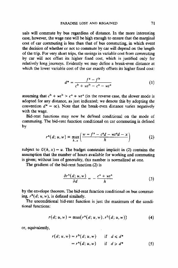
from (3). Thus the bid-rent function has a kink at d*, reflecting the switch to a faster mode of transportation at that location. A typical bid-rent function is drawn as Fig. 1.

3. RESIDENTIAL EQUILIBRIA-ZERO FIXED COSTS

We are now in a position to informally describe equilibrium residential patterns of different income groups and to determine how they vary with the material cost of the faster mode. Assume that two groups differing only in their income compete for housing in the city. Let w, be the wage of the rich and wP (< w,) be the wage of the poor. To illustrate the logic of our model, we first consider the case in which the fixed costs of both modes are zero. In that event, the break-even distance for a group is either zero or infinity, depending on whether the wage of that group is or is not high enough that the lower time cost of the faster mode offsets its higher material cost. Thus, if an income group uses a particular mode at one location, it does so at all locations. Now, suppose that the variable material cost of the faster mode falls steadily over time with respect to the wages of both groups. This assumption generates three different eras. In the first, the variable material cost of the car ca is so high that neither rich nor poor commute by car. In the second, ca is low enough to justify car commuting for the rich,

d’ d

FIG. 1. The bid-rent function.


but not for the poor. Finally, the third period is defined to occur when ca is so low that both the rich and the poor commute by car.

We now consider the equilibrium residential locations of the rich and poor in each of these three cases. Equilibrium locations will be the outcome of competition for housing among individuals in the same group and between groups. Competition for housing within either group will ensure that all individuals in that group have the same utility level regardless of location. Thus, the rents paid by either group will be consistent with the bid-rent function evaluated at one particular utility level, and competition among the groups and some alternative users such as farmers will determine the utility level for each group. Housing at any location will go to the group with the highest bid rent at that location, and the utility level for each group must be such that demand for housing per individual in each group is consistent with the number of individuals in that group and the supply of housing allocated to that group. When evaluated at equilibrium utility levels, the bid-rent functions of rich and poor will intersect at the boundary of the areas in which each income group lives. The group that lives on the side of that boundary closer to the CBD must have the steeper bid-rent function at that intersection. From (3) the poor will live on the CBD side of the boundary if and only if

cP + WP% c, + w,t,

h, ’ hr

where h, and h, are the housing consumptions of the poor and the rich, respectively, at the boundary. Here cp and t, are the variable material costs and travel times of whichever mode is taken by the poor, and c, and I, are the comparable parameters for the rich. The numerators of the fractions in (7) are the marginal commuting costs of the rich and the poor. Inequality (7) will therefore be satisfied if and only if the arc elasticity of housing consumption with respect to income q, exceeds the arc income elasticity of marginal commuting costs vlc.

Polinsky [ 171 and Polinsky and Ellwood [ 181 provided convincing evidence that the income elasticity of housing consumption is less than unity. The income elasticity of marginal commuting costs will depend on the modes used by both groups. When the variable material cost of car transportation is so high that both groups commute by bus, the cost of time spent commuting constitutes the major portion of marginal commuting costs. Accordingly, t is close to unity since the value of time rises proportionally with income. Thus, it is likely that TIN > TIN, so that the rich live on the CBD side of the boundary between rich and poor. We have the paradise era referred to in the introduction.


In the second period, ca is assumed to have fallen sufficiently that the rich commute by car, but not so much that the poor do so also. For the rich to live on the CBD side of a boundary between rich and poor, it is necessary and sufficient that

ca + w,t” hr ’

Cb + wprb h,

from inequality (7). Now, if both groups were commuting by the same mode at that intersection the corresponding condition would be satisfied by assumption. But by definition the poor commute by bus while the rich commute by car, and since for the rich the marginal commuting cost for the car is by assumption less than that for the bus, it is possible that at the boundary the bid-rent function of the rich is flatter than that of the poor even under the assumption of the preceding paragraph. In that event, which we suppose to obtain, the rich have a comparative advantage living on the suburban side of the boundary.

Finally, assume that ca falls further, so that the poor also commute by car. The income elasticity of marginal commuting cost again depends on the relative weights of time and material costs in commuting. As in the first period, we assume that the weight on time is high enough to ensure that 77, exceeds qi,, although that assumption is problematic in the present case because the car has higher material cost than the bus. Nevertheless, if the assumption is invoked the rich again live on the CBD side of a boundary between rich and poor, and we have the paradise regained era in which the rich return to downtowns.

4. RESIDENTIAL EQUILIBRIA-POSITIVE FIXED COSTS

The zero fixed costs assumed in the preceding section helped us to present a simple version of our model, but it is highly unrealistic. Especially for cars, such fixed costs as time-related depreciation, parking, and insurance are at least as great as use-related depreciation and gasoline, the major variable material costs. We therefore combine the analysis of mode choice in the presence of fixed as well as variable costs conducted in Section 2 with the theory of equilibrium residential locations of different income groups presented in Section 3. It will be seen that a much richer set of residential equilibria can be generated when fixed costs are reintroduced; also, some of the equilibria that are generated only under positive fixed costs-such as the regentrification equilibrium-are indispensable in thinking about real- world residential patterns.

Suppose that at firstfa and ca are high enough that d: = dc = 00. In this case, both the rich and the poor commute by bus, and the rich will live in


the downtown residential area under exactly those conditions analyzed in the preceding section (see Fig. 2). Assume now that f” and ca drop enough relative to incomes that the rich can economically commute by car, at least for sufficiently long commuting distances, but not so much that the poor also find car travel economical for commutes of any length. In terms of our model we are assuming that the relative costs of car commuting have fallen enough that d: lies well inside the boundary of the city, but that dp* is still either infinite or very high. The city can then be divided into two zones. In zone 1, defined by 0 < d < d:, both groups commute by bus, while in zone 2, defined by d > d :, the poor commute by bus but the rich by car. Of course, this classification does not tell us which income group lives at a particular location; it only describes the mode of transportation used by whichever group lives there. A boundary between the residential areas of the rich and the poor is possible in either zone 1 or 2. If the only boundary occurs in zone 1, as in the paradise equilibrium, the rich will live on the CBD side of that boundary under the maintained assumptions. But as f” and ca drop relative to wages, d: decreases and the supply of land available in zone 1 diminishes. At some point not enough land will remain to accommodate the housing demands of the rich; consequently, there must come into existence a boundary in zone 2. At such a boundary the rich will commute by car and the poor by bus, and therefore, as pointed out above, the bid-rent function of the rich may be flatter than that of the poor. In that event the rich will have a comparative advantage living on the suburban side of the boundary. We see that the decline in the material costs of car commuting will sooner or later lead some of the rich to buy cars and move

FIG. 2. Paradise.


to the suburbs (Fig. 3a). Note that the residential equilibrium just described, in which some of the rich commute by bus and some by car, and in which the downtown and far-suburban residential areas of the rich are separated by a near-suburban area populated by poor bus commuters, depends essentially on the presence of fixed costs, since we have the rich using different modes at different locations. Depending on parameter values, however, it may or may not be the case that all the rich will eventually move to the suburbs (as illustrated in Fig. 3b). Any residential equilibrium in which the outermost residential area is occupied by the rich using cars will be termed a paradise lost equilibrium, although the term evidently applies better to equilibria of the type indicated in Fig. 3b than to that shown in Fig. 3a.

But now assume that in the fixed and variable material cost of car transportation drops further. Evidently the comparative advantage of the rich in bearing high material cost is diminished. At some point the poor, commuting by car, will become the high bidders for land for suburban homes, again by virtue of the maintained assumption that the income elasticity of marginal commuting cost is greater than the income elasticity of housing demand when both groups use the same mode. Accordingly, a new boundary between the rich and the poor will occur in the region in which both groups commute by car. When this occurs, the paradise lost era will have ended, since the rich no longer occupy the urban periphery. With the rich becoming less effective in competing for housing in the suburbs, due to the decline in the material cost of car ownership, they must be competing

FIG. 3. Paradise lost.


relatively more effectively elsewhere, comparative advantage being what it is. The indicated area is, of course, the innermost urban residential area, where the rich also have a comparative advantage, since there both groups would commute by the same mode. This improvement in the competitive position of the rich in bidding for land in the innermost residential area will eventually establish them as dominant bidders (if they were not at the outset). Thus, the advent of the poor as car commuters in the outermost residential areas will be accompanied by a return of some of the rich to the downtown areas. We have the regentrification equilibrium depicted in Fig. 4. Again, a qualification is in order. Depending on the relative populations of rich and poor, the rich may not ever entirely evacuate the downtown under the paradise lost equilibrium, in which event regentrification would refer to an increase in the size of the innermost residential area occupied by the rich, rather than to the creation of such a region. It may seem puzzling that a decrease in the cost of car transportation induces some of the rich to give up their cars and move to the city. It is less so if one recalls that mode choice depends on location, which in turn depends on comparative and not absolute advantage. With this in mind, it is not surprising that a decrease in material transportation cost will induce some of the poor to buy cars and displace some of the rich in the suburbs, with the reverse occurring in the city center.

In choosing where to live, the rich and the poor do not think in terms of comparative advantage, of course, but simply do the best they can for themselves subject to incomes and prices. The poor see that a decrease in the variable material cost of car commuting means that they can get a car

4 db d

FIG. 4. Regentrification.


d; d; d

FIG. 5. Paradise regained.

and move to the suburbs where housing is cheaper. The rich, on the other hand, who were willing to commute long distances when suburban real estate was very inexpensive, now see that (because the poor are bidding for suburban housing) suburban housing prices have risen to the point that the differential between suburban and urban housing prices no longer justifies the high time cost of commuting. Some, therefore, move downtown, where the short commuting time offsets the somewhat higher cost of housing.

As the material cost of car transportation declines, the rich using cars will become increasingly effective bidders for the land occupied during the regentrification era by poor bus commuters; the latter, in turn, find it increasingly attractive to acquire a car and move to the distant suburbs. Eventually the poor will be entirely displaced in the intermediate region, resulting in a pattern in which the innermost residential area is occupied by rich bus commuters (as in the regentrification equilibrium), the intermediate region is occupied by rich car commuters, and the suburbs by poor car commuters. This new equilibrium, paradise regained, resembles the original paradise pattern in that all the rich reside in the area closest to the CBD, whereas all the poor live in the more distant areas of the city (Fig. 5).

5. THE HISTORICAL RECORD

We have presented a model that relates urban residential patterns to the availability of a fast mode of transportation that is cheap enough to be used economically by the rich but is too costly for the poor. To simplify drastically, when such a mode exists (paradise lost), the rich live in the suburbs and the poor downtown. When such a mode is not available, either


because the faster mode is too expensive even for the rich (paradise), or is cheap enough even for the poor (paradise regained), then the rich live downtown and the poor in the suburbs. In this section we demonstrate that to a striking extent the changes in residential patterns that actually occurred in American cities can be explained in the terms just set forth.

In the 18th and first half of the 19th centuries, almost all American city dwellers worked near the center of the city and walked to work; carriages were available, but only to the very rich. Cities in this era conformed to our paradise scenario, with carriages representing the rapid mode of transportation which is available, but which is too expensive for commuting except by a negligible minority. Since the variable material cost of walking to work is zero, the income elasticity of marginal commuting cost is unity, thus exceeding the income elasticity of housing demand. In this case our model predicts that the rich will live on the CBD side of the boundary. The historical records from that period indicate that, as predicted, household income declined with distance from the center. In 1849, for example, an observer wrote that “nine-tenths of those whose rascalities have made Philadelphia so unjustly notorious live in the dens and shanties of the suburbs.” 3

This contemporary characterization has been verified by modem historians. Using federal manuscript censuses and other data, Conzen [2] reconstructed the socioeconomic landscape of Milwaukee in 1850 and 1860. In Table 1 four indicators of income or wealth are presented by quarter-mile rings radiating outward from the Milwaukee CBD. For every index in both years income generally declined with distance from the CBD. Tarr [24] found the same pattern for Pittsburgh in 1850. The bulk of the economic activity of Pittsburgh (72% of the employees) was located in Wards One through Four, which were also the most prestigious residential areas. Seventy-eight percent of the bankers, merchants, manufacturers, and professionals of the city lived in this area, while only 48% of its skilled workers and 36% of its unskilled workers did so. Goheen’s [7] study of Victorian Toronto also confirmed this pattern. Using factor analysis, Goheen reduced a large body of data contained in the Toronto Assessment Roles to several significant factors and determined the variation in factor scores by location within Toronto. Since his statistical results are not easily summarized, we merely repeat his conclusions based on the analysis of the factor most closely related to economic status:

the center of the city was still, in 1860, an area of high prestige. This meant that not only was the city core still inhabited by businessmen enjoying high status but that the lowest economic class, the unskilled workers, were absent from it. These were

3This passage is quoted in Jackson [ 11, p. 1981.

80 LEROY AND SONSTBLIE

TABLE I

Socioeconomic Status in Milwaukee

Real Without Miles from property per servants

Year CBD household m ____--

1850 O-l/4 191.25 59.19 l/4-1/2 119.18 72.10 l/2-3/4 113.80 82.45 3/4-l 280.33 87.22

l-5/4 40.36 89.95 5/4-3/2 18.44 100.00

1860 o-1/4 487. I 1 61.17 l/4-1/2 532.03 71.82 l/2-3/4 655.12 72.73 3/4-I 247.64 78.24

l-5/4 85.33 93.49 5/4-3/2 65.98 94.82 3/2-7/4 43.85 96.99 7/4-2 36.44 95.00

2-9/4 34.08 97.43

_.- Professional and business

(W

13.94 13.22 10.10 6.38 3.66 0.00

19.57 16.87 16.34 7.84 3.85 2.57 2.49 1.33 2.56

Source. Conzen [2].

Laborers

m

11.90 15.03 24.09 36.54 3556 45.13

6.59 15.81 25.53 21.96 26.42 36.72 47.36 53.01 66.41

dispersed into the less accessible and, so it seems, less desirable districts of the city (P. 122)

These three studies support the prediction of our paradise scenario that when all workers commute by the same slow but inexpensive mode, walking in this case, the rich live closer to the CBD than the poor.

The first real alternative to walking as a mode of commuting was the omnibus, a horse-drawn vehicle carrying twelve passengers.4 The omnibus had its heyday from about 1830 to 1850. It was never cheap to ride, with fares ranging from 124 to as high as 5Oe at a time when a laborer might earn $1.00 a day. Further, the omnibus probably did not travel faster than 6 mi/hr. Its use as a means of commuting was therefore limited even among the wealthy. Nevertheless, historical reports indicate that it did have some effect on residential patterns. One observer of New York in 1846 reported that since his last visit to the city

whole streets had been built, and several squares finished in the northern or fashionable end of town, to which the merchants are now resorting, leaving the business end, near the Battery, where they formerly lived. Hence there was a

4The following account of the omnibus, the commuter railroad, and the streetcar is based on Taylor [25].


constant increase of omnibuses passing through Broadway, and other streets running north and ~outh.~

Commuter railroads also began operating in the 1830s. The noise and smoke of the steam locomotive made these railroads very unpopular, however, causing many cities to enact ordinances severely restricting their operation. This was particularly true in Philadelphia and New York, although Boston did have several lines by 1850. As with the omnibus, railroad fares were generally expensive; thus, the suburban communities spawned by the railroads were primarily havens for the very rich.6

When introduced, both the omnibus and the commuter railroad played the role of the faster mode in our model, and as the model predicts their introduction was quickly followed by some movement of the rich to the suburbs. This movement was very limited, however, at least in comparison with that engendered by the streetcar, which was introduced in American cities in the 1850s and 1860s. Streetcars were pulled by horses at first, but unlike the omnibus they ran on rails laid on city streets, making them both faster and more efficient than the omnibus. Whereas an omnibus required two horses to carry 12 passengers, a two-horse streetcar could easily carry 40 passengers at speeds at least one-third greater than that of the omnibus. Streetcar fares were generally 5e a trip, which was lower than the omnibus but still expensive for workers of that day.

Historians such as Warner [32] and Ward [31] take the view that the introduction of the streetcar caused the first major flight of the affluent to the suburbs. A recent study of the journey to work for Philadelphians in 1850 and 1880 supports that view.’ Law and bookbinding, occupations for which the workplaces were centrally located (as assumed for all occupations in our model), exemplified this pattern. In 1850, according to the study, 52% of the lawyers lived at their place of work and the median journey to work for those who did not combine work and residence was 0.2 mi. In contrast, only 30% of the bookbinders combined home and work, and the median distance of the journey to work for those who did not was 0.7 mi. By 1880, after the introduction of the streetcar, the number of lawyers that combined home and work had fallen to 188, while 9% of the bookbinders continued to do so. For our purpose, however, the significant fact is that the median length of the journey to work for lawyers was now greater than that for bookbinders: 1.3 as opposed to 1.1 mi. Thus the length of the journey to work increased for both bookbinders and lawyers, but that increase was much more dramatic for lawyers, suggesting that lawyers made more use of the streetcar to move to the suburbs than did the less affluent bookbinders.

‘Quoted in Taylor [25, Part I, p. 481. 6Tbe character of these railroad suburbs is described in Warner 132, pp. 58-601. ‘See Hershberg et al. [9].


TABLE 2 Commuting Mode of Male Workers in Lower Manhattan, 1907

Weekly wage

Walking Paying 106 carfare Paying more than to work or less per day 1 OC carfare per day

6) 6%) 6)

$8.00-$9.99 51.9 37.5 10.6 10.00-11.99 41.0 45.1 13.9 12.00-13.99 36.8 51.1 12.1 14.00-15.99 30.2 48.0 21.8 16.00-17.99 21.3 57.4 21.3 18.00-19.99 23.1 48.3 28.6 20.00-21.99 12.1 60.5 27.4 22.00-23.99 18.6 47.2 24.2 24.00-25.99 15.3 51.2 33.5

_ Source. Pratt [ 191.

-

The most convincing evidence for our paradise lost scenario comes from a 1907 survey of manufacturing workers in Manhattan.* Reported in Table 2 is the mode of commuting for men employed in manufacturing firms located below 14th Street in Manhattan. Note that the proportion that walked to work falls from 52% for those earning between $8 and $lO/week to 15% for those making between $24 and $26/week. There is also a steady increase in the proportion of those paying more than lOe/day in carfare as income increases. For the intermediate category, those paying lOC/day or less in carfare, there is no clear trend. The information in Table 3 indicates that higher-paid workers also generally lived farther from work. The proportion working in lower Manhattan who also lived there declined from 54% in the lowest wage group to 14% in the highest wage group. The higher-paid workers generally lived in the boroughs of New York other than Manhattan, and in New Jersey. Both tables indicate that lower-paid workers lived close to their place of employment and frequently walked to work, while higher- paid workers generally lived farther from work and commuted by streetcar. That is precisely the pattern of our paradise lost equilibrium.

The streetcar fare generally remained at the traditional 5t throughout the first decades of the 20th century. Consequently, as wages rose the streetcar became available to lower and lower income groups, If no new mode had been introduced, our theory would lead us confidently to expect a paradise regained era, perhaps in the 192Os, when the decline in carfare relative to wages had progressed to the point at which the streetcar had become practicable for all groups. As is well known, this did not occur, and the reason is equally well known: the introduction of the car.

‘See Pratt [ 191


TABLE 3 Residences of Male Workers Employed in Lower Manhattan, 1907

Weekly wage

$ 8.00-$9.99 10.00-11.99 12.00-13.99 14.00-15.99 16.00-17.99 18.00- 19.99 20.00-2 1.99 22.00-23.99 24.00-25.99

Manhattan Manhattan below 14th St. above 14th St.

cw (W

53.8 15.0 45.1 21.4 42. I 24.5 33.6 27.3 24.5 20.4 27.2 23.3 11.6 25.8 16.9 25.8 14.4 18.1

Other New boroughs Jersey

(W m

26.8 4.4 26.6 6.9 36.4 7.0 28.2 10.9 45.4 9.7 39.2 10.2 48.0 14.6 41.2 16.1 51.7 15.8

Source. Pratt [ 191.

The first homeless carriages were invented before the turn of the century, but car ownership did not become widespread until after Henry Ford introduced the Model T in 1908. Although the streetcar, which caused the first major wave of suburbanization by the affluent, was now within reach of every working family, the car surely was not. Accordingly, we speculate that the introduction of the car forestalled the shift to the paradise regained regime that would otherwise have occurred; instead it reinforced and renewed the paradise lost era. Now, however, the streetcar played the role of the slower mode with low material cost rather than of the rapid mode with high material cost, as it did in the initial period of suburbanization.

A committee commissioned by President Hoover to investigate current social trends characterized the effect of the car in this way.

The motor car, bringing the country nearer in time, has caused an unprecedented development of outlying and suburban residential subdivisions. While this development pertains to families of a wide range of income, special attention has been given in the past decade to the promotion of exclusive residential districts designed for occupancy by the higher income classes.9

The most comprehensive study of urban residential areas during the Depres- sion was that of Hoyt [lo] who found that in all but two of nineteen selected cities the high-income areas were located on the periphery.”

‘President’s Research Committee on Social Trends [20]. “We have assumed competitive conditions in discussing the choice of mode, but that

assumption may be subject to question. For the role of the General Motors Corporation in dismantling the streetcar systems of Los Angeles, New York, Philadelphia, Baltimore, St. Louis, Oakland, Salt Lake City, and other cities, see Snell [22].


6. REGENTRIFICATION

It is well known that the flight of the rich to the suburbs, generated, we contend, by the increasing ownership of cars, accelerated in the 1950s and 1960s. The much publicized urban crisis of the 1960s resulted from the nearly complete evacuation by the rich of the downtown areas of the large eastern and midwestem cities especially. But in the 1970s the pace of the outward movement of the rich slowed sharply, in some cases stopping altogether. The groups moving to the suburbs have increasingly been lower-income groups, rather than the rich as in the early stages of suburbanization. Also, a new phenomenon, the return of the rich to downtown residential areas, has become increasingly evident in the last few years. Although the trend began in the early 1970s it became sufficiently widespread to attract the attention of the media only relatively recently (see the articles in Newsweek [ 161 and Harper’s [8], and also Gale [5, 61.

All of this is, of course, exactly as would be expected during the transition from a paradise lost equilibrium to a regentrification equilibrium in the model of this paper. As the material cost of commuting by car declines beyond the interval consistent with a paradise lost equilibrium, increases in the incidence of car ownership are greatest in the lower income groups. These groups increasingly move to the suburbs and commute by car. Concomitantly, some rich suburbanites move downtown, making much less use of the car than those of comparable income who stay in the suburbs. The Washington, D.C., metropolitan area provides the most dramatic example of this regentrification pattern, with the downtown residential areas increasingly populated by rich professionals who walk or bicycle to work, while such suburban areas as Prince George’s County, Maryland, are receiving an influx of the poorer former residents of downtown Washington, DC., who, despite their low income, rely primarily on transportation by cars. Regentrification on a widespread scale is also evident in Boston, Philadelphia, Baltimore, Atlanta, Chicago, Detroit, and other cities.

Changes in commuting costs in the postwar era are consistent with our explanation for changes in residential equilibria. Measures of these costs are presented in Table 4 for the years 1950, 1960, 1970, and 1977. The variable material cost of car commuting is assumed to consist of expenses for gas, oil, and repairs and maintenance. Our estimates of these costs are based on a 1970 study of the costs of operating a car (U.S. Department of Transpor- tation [29]); data on gasoline prices, fuel efficiency, oil prices, and the CPI index for repairs and maintenance were used to adjust the 1970 figure for 1950, 1960, and 1977 (U.S. Department of Labor [28] and U.S. Department of Transportation [30]). We assumed that a single fare is charged for a bus ride regardless of distance, so that the variable material cost of the bus is zero.


TABLE 4 Parameter Values

Variable material cost BUS CX

Fixed cost Bus CX

Annual income Rich Poor

Variable time cost Rich

Bus Car

Poor Bus CLU

Break-even distance Rich

1950

0 2.08C/mi

$0.24/day $O.S8/day

$4896 $1855

8.07Q/mi 3.13c/mi

3.06Q/mi I.l9C/mi

5.9 mi 03

1960

0 2.61 t/mi

$0.43/day $0.73/day

$8257 $3265

13.614/mi 5.28Q/mi

5.38Q/mi 2.09b/mi

2.6 mi 22.1 mi

1970

0 3.24$/mi

$0.75/day $l.l3/day

$14,386 $5970

23.7lQ/mi 9.2lO/mi

9.84O/mi 3.82e/mi

1.7 mi 8.3 mi

1977

0 5.52e/mi

$l.OO/day $ I .5O/day

$23,993 $9278

39.54c/mi 15.36e/mi

15.29e/mi 5.94e/mi

1.3 mi 6.5 mi

Sources. U.S. Department of Transportation, Cost of Operating an Automobile, February 1970 [29]; U.S. Department of Transportation, National Transportation Statistics, Annual Report, August 1979 [30]; U.S. Bureau of the Census, Statistical Abstract of the United States, 1980 [26]; U.S. Department of Labor, Handbook of Labor Statistics, 1978 [28].

The fixed cost of car transportation includes time-related depreciation, interest, and insurance. But only a part of this cost can properly be charged against commuting, since personal cars have other important uses. Rather than attempt to deal with the formidable problem of determining what portion of fixed cost to impute to commuting, we simply chose an arbitrary value of $1.5O/day for the fixed cost of car transportation in 1977. That figure we then revised for 1950, 1960, and 1970 by applying the CPI index for new car prices. The fixed cost of bus transportation is the amount of busfare, which we set arbitrarily at 5Ot/ride in 1977 and adjusted for 1950, 1960, and 1970 by the CPI index for local transit fares. Thus, although the relative values of fixed transportation costs between 1950, 1960, 1970, and 1977 are measured, the scale in the level of these costs has been selected arbitrarily.

The change in these costs relative to the value of time is the key to our explanation. Commuters are assumed to value their time at 32% of their


wage, a value estimated by McFadden [ 141.’ ’ The time cost of car transportation in all four years was assumed to be 0.04 hr/mi, while the corresponding figure for the bus was 0.103 hr/mi.12 The wage rate of the rich and poor in each of the four years was determined by the income of families in the 75th and 25th percentile of the income distribution for that year (U.S. Bureau of the Census [26]), respectively. Using those parameter values, we calculated the cost of time per mile traveled for each mode and each income class. These calculations are presented in Table 4. Also shown in Table 4 are the break-even distances implied by these costs.

In 1950 the rich would have commuted by car for all distances greater than 5.9 mi, but the poor would not have done so for any distance. Given that the poor commute by bus and the rich by car, the arc elasticity of marginal commuting costs is 0.58. Polinsky and Ellwood [18] estimated the income elasticity of housing demand to be 0.57, with a standard error of 0.11. Because of certain peculiarities of their data, however, they expressed the view that this estimate should be increased by 40 to 50% which leads to a range of 0.80 to 0.87. Expanding this range by one standard error yields an interval of 0.69 to 0.98, which we take to be a reasonable interval for the income elasticity of housing demand. Since the arc elasticity of marginal commuting costs falls well below this range, the 1950 data clearly generate the paradise lost equilibrium that we have attributed to the early postwar era.

The same is true for the 1960 parameter values. The rich commute by car for all distances greater than 2.6 mi, while the break-even distance for the poor is 22.1 mi. Consequently, the rich will be predominantly car commuters and the poor will be bus commuters, just as in 1950. In this case the arc elasticity of marginal commuting cost is 0.44, which is well below the probable value for the income elasticity of housing demand. Thus the parameter values for 1960 lead to a similar equilibrium as those for 1950.

The parameter values for 1970 point to a different pattern, however. The break-even distance for the poor is now 8.3 mi, which means that the poor

“For simplicity in developing our model we have assumed that neither time spent commuting nor time spent working enters the utility function, implying that the opportunity cost of time spent commuting equals the wage. If either does enter the utility function, the value of time spent in commuting will in general differ from the wage. McFadden [14] and others found that empirically the opportunity cost of commuting appears to be less than the wage, and we have incorporated this fact in our calculations. Of course, there is no theoretical reason why commuting time should be valued at the same proportion of the wage for different incomes, although we have made that assumption. Recent work by Diamond [3] suggests that in fact the value of commuting time rises more than proportionally with the wage, in which case the income elasticity of marginal commuting cost would be higher than assumed in the following simulations, and thus the tendency for regentrification to occur would be more pronounced than our calculations indicate.

“These figures are based on data for commuting times and distances in U.S. Bureau of the Census, “Selected Characteristics of Travel to Work in 20 Metropolitan Areas: 1976” [27].


TABLE 5

Percentage of Households Owning Cars, by Income Quintile

Quintile

Year Lowest Second Third Fourth Highest

1952 26 44 64 19 89 1957 33 62 82 89 95 1962 32 65 16 91 94 1969 45 19 93 95 97 1977 61 89 95 97 97

Sources. 1962 Survey of Consumer Finances [ 121, 1970 Survey of Consumer Finances [ 131, Federal Reserve Board, 1977 [4].

would commute by car for distances typical of suburban locations. If both rich and poor commute by car, as would be true for such locations, the arc elasticity of commuting costs is 0.67. Since this is quite close to the likely range for the income elasticity of housing demand, the poor would have been in a position in 1970 to compete on roughly equal terms with the rich for suburban residential locations. Of course, this is the condition necessary for regentrification. The same conclusion applies for 1977. The break-even distances are even less, and the arc elasticity of marginal commuting cost is 0.66.

These results confirm the finding of Wheaton [33] that when both rich and poor commute by car, as in 1970 and 1977 in our calculations, the bid-rent functions of each are very close. No one group has a strong comparative advantage in either suburban or downtown locations. Where we differ with Wheaton, however, is in noting that in 1950 and 1960, when the poor did not find car commuting economical, the rich had a clear comparative advantage in suburban locations. The regentrification period marks the end of that pattern, due to the now widespread use of the car by the poor (see Table 5) and their consequent movement to suburban locations.

7. CONCLUSIONS

The present circumstance of American cities is historically anomalous. In the 150 years prior to the 1970s a clear pattern can be seen in the evolution of transportation technology and the associated equilibrium residential patterns. Successive innovations were always expensive at the time of their introduction, therefore giving the rich a comparative advantage in the suburbs, but these newer modes always ultimately became cheap enough for use by the poor. Before this decrease in the price of the newest mode of transportation could generate the reversal of residential patterns that would


otherwise have taken place, however, a new innovation in transportation would occur, resulting in a continuation (or, in the event, generally an intensification) of the tendency of the rich to live in the suburbs. As we have seen, the mode formerly used by the rich and subsequently superseded was then adopted by the poor. The present period is anomalous because the new mode to replace the car as the mode used by the rich called for in the preceding script has not yet emerged, although by historical comparison it is long overdue, so the reversal in residential housing patterns that has always been forestalled by the adoption of the new mode is now in fact happening.

Will the regentrification of American cities continue? Our model suggests an affirmative answer if (1) no new, faster mode of commuting appears, and (2) the real material cost of car commuting continues to decline. With regard to the latter, the outlook is not clear. On the basis of such casual evidence as the recent increases in nominal car prices due to the mandating of safety equipment and pollution controls, it appears unlikely that the pronounced decline in the fixed (private) cost of cars relative to incomes noted in Table 4 can continue. The real variable material cost of car transportation-that is, principally the real price of gasoline-has, of course, risen dramatically. l3 It is widely supposed that this change is good for the downtown areas of cities and bad for their suburbs. This is true in the sense that high gasoline prices lead to greater concentration of the entire urban population near the CBD, implying increases in downtown rents and decreases in suburban rents. But high gasoline prices also increase the comparative advantage of the rich in the suburbs, since the rich are better able to bear high material costs than the poor. In terms of our model, an increase in variable material cost decreases the income elasticity of marginal cost of car commuting which, as we have seen above, is associated with the movement of the rich to the suburbs. Thus our model suggests that increases in gasoline prices discourage regentrification, rather than encourage it as is widely believed.

REFERENCES 1. W. Alonso, “Location and Land Use,” Harvard Univ. Press, Cambridge, Mass. (1964). 2. K. N. Conzen, Patterns of residence in early Milwaukee, In “The New Urban History:

Quantitative Explorations by American Historians,” (L. F. Schnore, Ed.), Princeton, Univ. Press, Princeton N.J. (1975).

3. D. B. Diamond, Jr., Income and residential location: Muth revisited, Z/&n Studies, 17, 1-12 (1980).

4. Federal Reserve Board, “1977 Consumer Credit Survey” Washington, D.C. (1978). 5. D. E. Gale, “The Back to the City Movement,” Occasional Paper Series, Department of

Urban and Regional Planning, The George Washington Univ., Washington, D.C. (September 1976).

6. D. E. Gale, “The Back to the City Movement Revisited,” Occasional Paper Series,

130f course, the impact of higher gasoline prices might be largely offset by increased fuel efficiency.


Department of Urban and Regional Planning, George Washington Univ., Washington, D. C. (September 1977).

7. P. G. Goheen, “Victorian Toronto, 1850 to 1900: Patterns and Process of Growth,” Research Paper 127, Dept. of Geography, Univ. of Chicago, Chicago (1970).

8. Harper’s (December 1978). 9. T. Hershberg, H. Cox, D. Light, Jr., and R. R. Greenfield, “The Journey-to-Work: An

Empirical Investigation of Work, Residence and Transportation in Philadelphia between 1850 and 1880,” Philadelphia Social History Project, Univ. of Pennsylvania, Philadelphia (March 1979).

10. H. Hoyt, “The Structure and Growth of Residential Neighborhoods in American Cities,” U.S. Gov. Printing Office, Washington, D.C. (1939).

I 1. K. T. Jackson, The crabgrass frontier: 150 years of suburban growth in America, In “The Urban Experience: Themes in American History” (R. A. Mohl and J. F. Richardson, Eds.), Wadsworth, Belmont, Calif. (1973).

12. G. Katona, C. A. Lininger, and R. F. Kosobud, “1962 Survey of Consumer Finances,” Univ. of Michigan Survey Research Center, Ann Arbor, Mich. (I 963).

13. G. Katona, L. Mandel, and J. Schmiedeskamp, “1970 Survey of Consumer Finances,” Univ. of Michigan Survey Research Center, Ann Arbor, Mich. (1971).

14. D. McFadden, “The measurement of urban travel demand,” J. Public Econ., 3, 303-328 (1974).

15. R. F. Muth, “Cities and Housing,” Univ. of Chicago Press, Chicago (1969). 16. Newsweek (January 15, 1979). 17. A. M. Polinsky, The demand for housing: A study in specification and grouping,

Econometrica, 45, 447-461 (1977). 18. A. M. Polinsky, and D. T. Ellwood, Empirical reconciliation of micro and grouped

estimates of the demand for housing, Rev. Econ. Statist., 61, 199-205 (1979). 19. E. E. Pratt, “Industrial Causes of Congestion of Population in New York City,” Ph.D.

Dissertation, Columbia Univ. (1911). 20. “Recent Social Trends in the United States: Report of the President’s Research Committee

on Social Trends,” McGraw-Hill, New York (1934). 21. M. G. Reid, “Housing and Income,” Univ. of Chicago Press, Chicago ( 1%2). 22. B. C. Snell, “American Ground Transportation: A Proposal for Restructuring the Automo-

bile, Truck, Bus and Rail Industries,” U.S. Gov. Printing Office, Washington, D.C. (1974).

23. G. J. Stigler, and G. S. Becker, De gustibus non est disputandum, Amer. Econ. Reu., 67, 76-90(1972x

24. J. A. Tarr, “Transportation Innovation and Changing Spatial Patterns in Pittsburg 1850-1934,” Public Works Historical Society, Chicago (1978).

25. G. R. Taylor, The Beginnings of Mass Transportation in Urban America, Parts I and II,” Smithsonian Journal of History I (Summer and Autumn, 1966): 35-50 and 31-54.

26. U.S. Bureau of the Census, “Statistical Abstract, 1980.” 27. U.S. Bureau of the Census, “Selected Characteristics of Travel to Work in 20 Metropolitan

Areas: 1976.” 28. U.S. Department of Labor, “Handbook of Labor Statistics, 1972, 1977, 1978.” 29. U.S. Department of Transportation, “Cost of Operating an Automobile (February 1970).” 30. U.S. Department of Transportation, “National Transportation Statistics, Annual Report,

August 1979.” 31. D. Ward, “Cities and Immigrants: A Geography of Change in Nineteenth-Century

America,” Oxford Univ. Press, New York (1971). 32. S. B. Warner, Jr., “Streetcar Suburbs: The Process of Growth in Boston, 1870-1900,”

Harvard Univ. Press, Cambridge, Mass. (1962). 33. W. C. Wheaton, Income and urban residence: An analysis of consumer demand for

location, Amer. Econ. Rev., 67, 620-63 I (1977).

Paradise Lost and Regained: Transportation Innovation...

Documents

Transcript of Paradise Lost and Regained: Transportation Innovation...