paper2col - Semantic Scholar · Develop an aeroelastic analysis for a double wedge airfoil in...

July 31, 2002 11:56

Proceedings of IMECE’022002 ASME International Mechanical Engineering Congress and Exposition

November 17-22, 2002, New Orleans, Louisiana, USA

IMECE/2002-32943

MODELING APPROACHES TO HYPERSONIC AEROELASTICITY

B.J. Thuruthimattam, P.P. Friedmann�, J.J. McNamara and K.G. Powell

Department of Aerospace EngineeringUniversity of Michigan

Ann Arbor, Michigan 48109-2140Email: [email protected]

ABSTRACTThe hypersonic aeroelastic problem of a double wedge air-

foil typical cross-section is studied using three different unsteadyaerodynamic loads: (1) third order piston theory, (2) Euler solu-tion, and (3) unsteady Navier-Stokes aerodynamics. Computa-tional aeroelastic response results are obtained, and comparedwith piston theory solutions for a variety of flight conditions.Aeroelastic behavior is studied for 7 � M � 15 at an altitude of70,000 feet. A parametric study of offsets and wedge angles isconducted. Piston theory and Euler solutions are fairly close be-low the flutter boundary, and differences increase with increase inMach number, close to the flutter boundary. Differences betweenviscous and inviscid aeroelastic behavior can be substantial. Theresults presented serve as a partial validation of the CFL3D codefor the hypersonic flight regime.

NOMENCLATUREa Nondimensional offset between the elastic axis and the mid-

chorda∞ Speed of soundb Semi-chordc Reference length, chord length of double wedge airfoilCL � CD � CMy Coefficients of lift, drag and moment about the y-

axisCp � PT � Cp � NS Piston theory pressure coefficient, and CFD

Navier-Stokes pressure coefficient respectivelyf � x � Function describing airfoil surfaceh Airfoil vertical displacement at elastic axis

�Address all correspondence to this author.

Iα Mass moment of inertia about the elastic axisKα � Kh Spring constants in pitch and plunge respectively; Kα �

Iαω2α � Kh � mω2

hL Lift per unit spanM Free stream Mach numberM � K Generalized mass and stiffness matrices of the structurem Mass per unit spanMEA Moment per unit span about the elastic axisnm Number of modes usedp PressureQ Generalized force vector for the structureQi Generalized force corresponding to mode iq∞ Dynamic pressureqi Modal amplitude of mode irα Nondimensional radius of gyrationS Surface area of the structureSα Static mass moment of wing section about elastic axisT Kinetic energy of the structuret Timeth Airfoil half thicknessU Potential energy of the structureV Free stream velocityvn Normal velocity of airfoil surfacexα Nondimensional offset between the elastic axis and the

cross-sectional center of gravityx � y � z Spatial CoordinatesZ � x � y � t � Position of structural surfaceα Airfoil pitch displacement about the elastic axisγ Ratio of specific heatsµm Mass ratio

1 Copyright 2002 by ASME

ρ Air densityωα � ωh Natural frequencies of uncoupled pitch and plunge mo-

tionsω1 � ω2 Natural frequencies of double wedged airfoilφi Mode shape for mode i

τ Thickness ratio; τ � thb

˙� � � ¨� � First and second derivatives with respect to time� � u � � � l Of the upper and lower surface, respectively

INTRODUCTION AND PROBLEM STATEMENTIn recent years, renewed activity in hypersonic flight re-

search has been stimulated by the current need for a lowcost, single-stage-to-orbit (SSTO) or two-stage-to-orbit (TSTO)reusable launch vehicle (RLV) and the long term design goalof incorporating air breathing propulsion devices in this classof vehicles. The X-33, an example of the former vehicle type,was a 1/2 scale, fully functional technology demonstrator for thefull scale VentureStar. Another ongoing hypersonic vehicle re-search program is the NASA Hyper-X experimental vehicle ef-fort. Other activities are focused on the design of unmanned hy-personic vehicles that meet the needs of the US Air Force. Thepresent study is aimed at enhancing the fundamental understand-ing of the aeroelastic behavior of vehicles that belong to this cat-egory and operate in a typical hypersonic flight envelope.

Vehicles in this category are based on a lifting body design.However, stringent minimum-weight requirements imply a de-gree of fuselage flexibility. Aerodynamic surfaces, needed forcontrol, are also flexible. Furthermore, to meet the requirementof a flight profile that spans the Mach number range from 0 to 15,the vehicle must withstand severe aerodynamic heating. Thesefactors combine to produce unusual aeroelastic problems thathave received only limited attention in the past. Furthermore,it is important to emphasize that testing of aeroelastically scaledwind tunnel models, a conventional practice in subsonic and su-personic flow, is not feasible in the hypersonic regime. Thus, therole of aeroelastic simulations is more important for this flightregime than in any other flight regime.

Previous studies in this area can be separated into severalgroups. The first group consists of studies focusing on panelflutter, which is a localized aeroelastic problem representing asmall portion of the skin on the surface of the hypersonic vehi-cle. Hypersonic panel flutter has been studied by a number ofresearchers, focusing on important effects such as aerodynamicheating [1], composite [2,3] and nonlinear structural models [4],and initial panel curvature [5]. A comprehensive review of thisresearch can be found in a recent survey paper [6]. A funda-mental question associated with these studies, is whether pistontheory, which has been widely used in the Mach number range,1.8 � M � 5.0 is an appropriate tool for modeling unsteady aero-dynamic loads on the surface of a hypersonic vehicle. This was

considered in Ref. [5], where the unsteady pressure coefficienton the surface of a typical panel, undergoing prescribed oscil-lations at frequencies representative of a typical panel in hyper-sonic flow, was computed using: third-order piston theory, anexact solution of the nonlinear Euler equations, and a numericalsolution of the unsteady Navier-Stokes equations. At a typicalhypersonic Mach number (M=10), results from the third-orderpiston theory are within 5% of the exact solution of the Eulerequations. However, a difference of approximately 60% existsbetween the Euler solution and the solution based on the Navier-Stokes equations. This implies that the accurate representationof the unsteady aerodynamic loading, at certain flight conditions,will require the solution of the Navier-Stokes equations. Anotherimplication of this statement is that the heat transfer problem mayhave to be coupled with the aeroelastic analysis of a hypersonicvehicle for certain portions of the flight envelope.

The second group of studies in this area was motivated bya previous hypersonic vehicle, namely the National AerospacePlane (NASP). Representative studies in this category are Refs.[7-11]. However, some of these studies dealt with the transonicregime, because it was perceived to be a critical region and theNASA Langley facilities (the Transonic Dynamics Wind Tunnel)were appropriate for testing vehicle behavior in this Mach num-ber range. In Ref. [9], Spain et al. carried out a flutter analysisof all-moveable NASP-like wings with slab and double wedgeairfoils. They found that using effective shapes for the airfoilsobtained by adding the boundary layer displacement thickness tothe airfoil thickness improved the overall agreement with exper-iments.

The third group of studies is restricted to recent papers thatdeal with the newer hypersonic configurations such as the X-33or the X-34. Reference [12] considered the X-34 launch vehi-cle in free flight at M=8.0, and then reinterpreted these resultsat different flight conditions using dynamic pressure and altitudecorrections. The aeroelastic instability of a generic hypersonicvehicle, resembling the X-33, was considered in Ref. [13]. Itwas found that at high hypersonic speeds and high altitudes, thehypersonic vehicle is stable, when piston theory is used to repre-sent the aerodynamic loads. Sensitivity of the flutter boundariesto vehicle flexibility and trim state were also considered [13]. Inanother reference [14], CFD-based flutter analysis was used forthe aeroelastic analysis of the X-43 configuration, using systemidentification based order reduction of the aerodynamic degreesof freedom. Both the structure and the fluid were discretizedusing the finite element approach. It was shown that piston the-ory and ARMA Euler calculations predicted somewhat similarresults.

From the studies on various hypersonic vehicles (Refs.[7, 14–16]), one can identify operating envelopes for each ve-hicle. One can obtain a convenient graphical representation ofoperating conditions for this class of vehicles, shown in Fig. 1,by combining these envelopes.


0

50,000

100,000

150,000

200,000

250,000

300,000

0 5 10 15 20 25 30Mach Number

Alt

itu

de

(ft)

NASP

X-33

X-34

X-43A

Figure 1. OPERATING ENVELOPES FOR SEVERAL MODERN HY-

PERSONIC VEHICLES.

In a recent study [17], the authors of this paper developedan aeroelastic analysis capability for generic hypersonic vehi-cles in the Mach number range 0 � 5 � M � 15, using compu-tational aeroelasticity. The computational tool consisted of theCFL3D code, developed by NASA Langley, combined with afinite element model of a generic hypersonic vehicle utilizingNASTRAN. During the validation process of the analysis [17],the authors studied the aeroelastic behavior of a two dimensionaldouble wedge airfoil, operating in the Mach number range of2 � 0 �

M� 15 � 0. It was found that the double wedge airfoil is

an excellent vehicle for studying aeroelastic behavior in hyper-sonic flow. Therefore, the current paper is aimed at studyingseveral important aspects of computational hypersonic aeroelas-ticity based on the double wedge airfoil. The specific objectivesof this paper are:

1. Develop an aeroelastic analysis for a double wedge airfoil inhypersonic flow using third-order piston theory.

2. Determine the time-step requirements for the reliable com-putation of the unsteady airloads for this particular problemwhen using the Euler and Navier-Stokes options of CFL3D.

3. Compare the aeroelastic behavior predicted by the simplepiston theory analysis with refined solutions for the sameproblem, using CFL3D, with both Euler and Navier-Stokessolutions for the unsteady aerodynamic loads.

4. Compare the exact solutions for aeroelastic behavior usingthe Navier-Stokes-based unsteady airloads, with approxi-mate solutions based on an airfoil shape modified by thepresence of a boundary layer.

5. Conduct a parametric study that illustrates the effect of off-sets between elastic axis, aerodynamic center and wedge an-gle of the airfoil.

Finally, it is important to note that these objectives not

only enhance our understanding of hypersonic aeroelasticity, butalso make a valuable contribution towards the validation of theCFL3D code for hypersonic flight conditions.

METHOD OF SOLUTIONAn overview of the solution of the computational aeroelas-

ticity problem is shown in Fig. 2. First, the vehicle geometryis created using CAD software, and from this geometry a meshgenerator is used to create a structured mesh for the flow domainaround the body. In parallel, an unstructured mesh is created forthe finite element model of the structure using the same nodes onthe vehicle surface that were used to generate for the fluid mesh.Subsequently, the fluid mesh is used to compute the flow aroundthe rigid body using a CFD solver, while the structural mesh isused to obtain the free vibration modes of the structure by fi-nite element analysis. Matching surface nodes in both meshesby their coordinates, the modal displacements at each fluid nodeare set to those of the appropriate node on the structural mesh,and thus the mode shape data for CFL3D is generated. Using theflow solution as an initial condition, and the modal information,an aeroelastic steady state is obtained. Next, the structure is per-turbed in one or more of its modes by an initial modal velocitycondition, and the transient response of the structure is obtained.To determine the flutter conditions at a given altitude, aeroelastictransients are computed at several Mach numbers and the corre-sponding dynamic pressures. The frequency and damping char-acteristics of the transient response at each Mach number can bedetermined from a moving block approach [18], and the flutterMach number associated with this altitude can be estimated byinterpolation.

Euler/Navier-Stokes Aeroelastic Option in CFL3DThe aeroelastic analysis of the double wedge airfoil is car-

ried out using the CFL3D code [19]. The code uses an implicit,finite-volume algorithm based on upwind-biased spatial differ-encing to solve the time-dependent Euler and Reynolds-averagedNavier-Stokes equations. Multigrid and mesh-sequencing areavailable for convergence acceleration. The algorithm, which isbased on a cell-centered scheme, uses upwind-differencing basedon either flux-vector splitting or flux-difference splitting, and cansharply capture shock waves. For applications utilizing the thin-layer Navier-Stokes equations, different turbulence models areavailable. For time-accurate problems using a deforming mesh,an additional term accounting for the change in cell-volume isincluded in the time-discretization of the governing equations.Since CFL3D is an implicit code using approximate factoriza-tion, linearization and factorization errors are introduced at ev-ery time-step. Hence, intermediate calculations referred to as“subiterations” are used to reduce these errors. Increasing thesesubiterations improves the accuracy of the simulation, albeit at


Geometry ( CAD software)

Mesh Generator

structuraldomain mesh

flow domainmesh

Finite elementanalysis

AeroelasticSolver

Postprocessing(flutter boundary)

Aeroelastictransientresponse

modes,frequency

flow overrigid body

CFDsolver

Figure 2. A FLOW DIAGRAM OF THE COMPUTATIONAL AEROELAS-

TIC SOLUTION PROCEDURE.

increased computational cost.The aeroelastic approach underlying the CFL3D code is

similar to that described in Refs. [20, 21]. In this formulation,the equations are derived by assuming that the general motionw � x � y � t � of the structure is described by a separation of time andspace variables in a finite modal series. The free vibration modesin this study were obtained from a finite element model of thevehicle. The displacements on the vehicle are obtained from amodal series, given next.

Z � x � y � t � �nm

∑i � 1

qi � t � φi � x � y � (1)

The equations of motion are based on Lagrange’s equations,

ddt

�∂T∂qi �� ∂T

∂qi � ∂U∂qi

� Qi � i � 1 � 2 � � � � (2)

The resulting set of equations of motion is

Mq � Kq � Q � q � q � q � � qT �� q1 q2 � � � � (3)

where the elements of the generalized force vector are given by,

Qi � ρV 2

2c2

Sφi

∆p dSρV 2 2 c2 (4)

From Eq. (3),

q � � M � 1Kq � M � 1Q (5)

The aeroelastic equations are written in terms of a lin-ear state-space equation (using a state vector of the form� � � � qi � 1 qi qi qi � 1 � � � � T ) such that a modified state-transition-matrix integrator can be used to march the coupled fluid-structural system forward in time. The fluid forces are coupledwith the structural equations of motion through the generalizedaerodynamic forces. Thus, a time-history of the modal displace-ments, modal velocities and generalized forces is obtained.

The aeroelastic capabilities of CFL3D, based on this modalresponse approach for obtaining the flutter boundary, have beenpartially validated for the transonic regime for the first AGARDstandard aeroelastic configuration for dynamic response, Wing445.6. The results of flutter calculations using Euler aerodynam-ics are given in Ref. [22] and those using Navier-Stokes aerody-namics are given in Ref. [23].

Computational Model of the Double Wedge AirfoilValidation of the CFL3D code for the hypersonic regime has

never been undertaken. Therefore, reliable results for a fairlysimple configuration for which aeroelastic stability and responseresults could be generated independently, were essential. A typ-ical cross-section based on the double wedge airfoil, shown inFigs. 3 and 4, met these requirements. Generating results for thisconfiguration using Euler and Navier-Stokes unsteady aerody-namic loads, and comparing them with results obtained using anindependently developed aeroelastic code based on third-orderpiston theory, provides a reliable means for validating CFL3D inthe hypersonic regime.

The Euler and Navier-Stokes computations are carried outusing a 225 65 C-grid with 225 points around the wing andits wake (145 points wrapped around the airfoil itself), and 65points extending radially outward from the airfoil surface. Thecomputational domain extends one chord-length upstream andsix chord lengths downstream, and one chord length to the up-per and lower boundaries. For the Navier-Stokes simulations,the Spalart-Allmaras turbulence model was used, along with anadiabatic wall temperature condition. The double wedge airfoiland a portion of the surrounding computational grid are shownin Fig. 3.

Aeroelastic Model for a Double Wedge Airfoil UsingHigher Order Piston Theory

Piston theory is an inviscid unsteady aerodynamic the-ory, used extensively in supersonic and hypersonic aeroelasticity,which provides a point-function relationship between the localpressure on the surface of the vehicle and the component of fluid


X

Y

-5 0-5

-4

-3

-2

-1

0

1

2

3

4

5

Figure 3. DOUBLE WEDGE AIRFOIL SECTION, AND SURROUNDNIG

GRID, TO SCALE.

a

ba

h

bxa

Kh

Ka

V

2th

2b

z

x

b

Figure 4. TWO DEGREE-OF-FREEDOM TYPICAL AIRFOIL GEOME-

TRY.

velocity normal to the moving surface [24, 25]. The derivationutilizes the isentropic ”simple wave” expression for the pressureon the surface of a moving piston,

p � x � t �p∞

��

1 � γ � 12

vn

a∞ �2γ�

γ � 1 �(6)

where

vn � ∂Z � x � t �∂t � V

∂Z � x � t �∂x

(7)

The expression for piston theory is based on a binomial ex-pansion of Eq. (6), where the order of the expansion is deter-

mined by the ratio ofvn

a∞. Reference [25] suggested a third-order

expansion, since it produced the smallest error of the various or-ders of expansion used when compared to the limiting values ofpressure, namely the ”simple wave” and ”shock expansion” so-lutions. The third-order expansion of Eq. (6) yields

p � x � t � � p∞ � p∞

�γ

vn

a∞ � γ � γ � 1 �4

�vn

a∞ � 2 � γ � γ � 1 �12

�vn

a∞ � 3 �(8)

An aeroelastic analysis for a typical cross-section for a dou-ble wedge airfoil was developed using Eq. (8) for the unsteadypressure loading. A typical cross-section, with the usual pitchand plunge degrees of freedom, shown in Fig. 4, was used toobtain the equations of motion from Lagrange’s equations.

mh � Sαα � Khh � � L � t �

Sαh � Iαα � Kαα � MEA � t �(9)

From Fig. 4, it is evident that for small displacements,

Z � x � t � � �� h � t � � � x � ba � α � t �� f � x � (10)

and

vn � u � �� h � � x � ba � α � � V � α � ∂ f � x �∂x �

vn � l � � h � � x � ba � α � � V � α � ∂ f � x �∂x � (11)

where

∂ fu � x �∂x � τ : � b � x � 0

∂ fu � x �∂x � � τ : 0 �

x�

b

∂ fl � x �∂x � � τ : � b

�x

� 0

∂ fl � x �∂x � τ : 0 � x � b

(12)

From Eqs. (8), (11), and (12) the unsteady pressure distributionwas determined. The unsteady lift and moment due to this pres-sure distribution was determined from

L � t � � � b� b � pl � x � t � � pu � x � t � � dx

MEA � t � � � � b� b � x � ba � � pl � x � t � � pu � x � t � � dx

(13)


The unsteady lift is given by

L � t � � L1 � t � � L2 � t � � L3 � t � (14)

where,

L1 � t � � 4P∞γMb � hV � ba α

V � α �L2 � t � � � P∞γ � γ � 1 � M2b2τ � α

V �L3 � t � � 1

3 P∞γ � γ � 1 � M3b �� hV � ba α

V � α �� hV � ba α

V � α � 2 � 3τ2 � � b αV � 2 � �

(15)

Note that L1 � t � , L2 � t � , and L3 � t � represent the first, second, andthird-order piston theory lift components respectively. Similarly,the unsteady moment is given by,

MEA � t � � M1 � t � � M2 � t � � M3 � t � (16)

where

M1 � t � � 4P∞γMb2 � a hV � � b

3 � ba2 � αV � aα �

M2 � t � � P∞γ � γ � 1 � M2b2τ � hV � 2ba α

V � α �M3 � t � � � 1

3 P∞γ � γ � 1 � M3b2 � 15 � b α

V � 3

� a � hV � ba α

V � α � � � hV � ba α

V � α � 2 � 3τ2 �� b α

V

� � hV � ba α

V � α � 2 � τ2

� ba αV � h

V � ba αV � α ��

(17)

Again, M1 � t � , M2 � t � , and M3 � t � represent the first, second, andthird-order piston theory moment components respectively.

For comparison with CFL3D, it is convenient to representEq. (9) in terms generalized coordinates and forces. Therefore, anormal mode transformation is used such that:

h � t �α � t � � � � φ1 φ2 � q1 � t �

q2 � t � � (18)

Substituting Eq. (18) into Eq. (9), and premultiplying by thetranspose of the modal matrix yields

q1 � t �q2 � t � � � � φ1 φ2 � T L � t �

MEA � t � � � �ω2

1 00 ω2

2 q1 � t �q2 � t � �

(19)for mass normalized modes.

Note that the modal amplitudes are coupled through the gen-eralized forces. Equation (19) was solved using the subroutineODE45 in MATLAB.

Calculation of Effective Shape of the Double WedgeAirfoil

As indicated in Ref. [26], the thick boundary layer in hy-personic flow can exert a major displacement effect on the outerinviscid flow, causing a given body shape to appear much thicker.This influences the surface pressure distribution, and it also ef-fects vehicle aeroelastic stability. To incorporate this effect inan approximate manner, a static boundary layer displacementthickness is used in conjunction with piston theory. A similarapproach was considered in Ref. [9], where a flat-plate bound-ary layer thickness was used. In order to improve the level ofaccuracy in the displacement thickness, the steady pressure dis-tribution calculated from a CFD based Navier-Stokes solution isused to generate the effective airfoil shape. The steady compo-nent of the piston theory pressure can be obtained from Eq.(8)by neglecting all time dependent terms. For zero angle of attack,this is given by:

Cp � PT � x � � p∞

q∞ γM

dZdx � γ � γ � 1 �

4M2 dZ

dx

2 � γ � γ � 1 �12

M3 dZdx

3 �(20)

Equating the steady CFD Navier-Stokes coefficient of pressure

with Eq.(20) yields a third order polynomial fordZdx

,

Cp � PT � x � � Cp � NS � x � � 0 (21)

Solving this equation at each surface grid point results in twocomplex roots and one real root, which represents the slope of theeffective airfoil shape at that grid point. The effective shape canthen be obtained by integrating the slope along the length of theairfoil.

RESULTS AND DISCUSSIONThe results presented in this section provide a validation of

CFL3D for the hypersonic regime, and also contribute to the fun-damental understanding of hypersonic aeroelasticity. By com-paring results for Euler, Navier-Stokes and piston theory, one canidentify the importance of viscosity, and the effectiveness of pis-ton theory in approximating the aeroelastic behavior of a doublewedge airfoil in inviscid flow.

The double wedge airfoil is characterized by the followingparameters: th b � 0 � 025; m � 51 � 833 kg/m; ωh � 50 rad/sec;and ωα � 125 rad/sec. Figure 5 depicts the flutter boundaries ofa double wedge airfoil at various altitudes, as a function of theoffset a, for the operating envelope of a typical hypersonic ve-hicle, at zero angle of attack, based on piston theory. The massratios for the various altitudes are given in Table 1. Two dif-ferent configurations of the double wedge airfoil, given in Table2, were selected for calculations using CFL3D. For flight in the


Mach number range of 5-15, the height selected for the fluttercalculations of the two configurations was 70,000 feet. At thisaltitude, the flutter boundaries are at M=9.21 for configuration Aand at M=14.55 for configuration B. Hence, appropriate compu-tational points selected for this study were Mach numbers 7, 10and 15 at 70,000 feet, with Reynolds numbers of 5 � 058 106,7 � 226 106 and 1 � 084 107, respectively.

a

Mac

hnu

mbe

r

-0.4 -0.2 0 0.2 0.40

5

10

15

20

25

30

35

40sea level5000 feet50,000 feet70,000 feet100,000 feet

Figure 5. FLUTTER BOUNDARIES OF A DOUBLE WEDGE AIRFOIL

AT ZERO ANGLE OF ATTACK, WITH xα � 0 � 2.

Table 1. MASS RATIOS AT VARIOUS ALTITUDES.

Altitude (ft) Mass Ratio (µm)

0 13.47

5,000 15 � 63

50,000 88 � 37

70,000 232.68

100,000 942 � 60

Selection of Time-step SizeThe time-step required for accurate prediction of the aeroe-

lastic response is important in computational aeroelasticity stud-ies. However, selection of an extremely small time-step alsorequires significant computational resources. Therefore the op-timal time-step, determined by a trade-off between accuracyand practical feasibility, was established by a concise numericalstudy.

Table 2. NONDIMENSIONAL GEOMETRIC AND STRUCTURAL PA-

RAMETERS.

Parameter Configuration A Configuration Bωh

ωα0 � 4 0 � 4

xα 0 � 2 0 � 2

rα 0 � 5 0 � 5

a 0 � 1 � 0 � 2

In an aeroelastic system with a linear structural operator, thetime-step limitation is mainly governed by the unsteady fluid cal-culations. Therefore, a simulation based on prescribed motionwas used to select an appropriate time-step size for each of theflight conditions. To determine the proper step size, the unsteadylift, moment and drag coefficients (CL � t � , CMy � t � and CD � t � ), dueto prescribed motion were computed, and the time-step selectedwas based on the convergence of these unsteady aerodynamiccoefficients. In studying the behavior of these coefficients whilevarying the step size, it was found that the lift coefficient CL hasthe smallest degree of sensitivity to the time-step. For aeroelas-tic simulations, the lift is the dominant quantity (since drag doesnot appear in the aeroelastic calculations for the double wedgeairfoil). Therefore, it might be expected that the time-step sizeshould be determined primarily based on the behavior of the CL

curves. For the double wedge airfoil geometry, the moment dueto lift (CL � xα) has the same order of magnitude as the momentcoefficient, and hence the accuracy of CMy is comparable in im-portance to the accuracy in CL.

For simulations using Euler aerodynamics, the responseswere found to be independent of time-step size when the time-step was smaller than 0.001 sec. To identify the maximum time-step for a viscous aeroelastic simulation, a maximum time-stepfor a viscous forced-motion simulation was found. This valueset an upper limit for the time-step size used in the aeroelasticsimulations. Simulations were carried out at 10, 20 and 30 Hz,with a maximum rotation of 1

�and 2

�, at various altitudes. Re-

sults from simulations carried out at 70,000 feet and Mach 10,with maximum rotation of 2

�at 20 Hz, are shown in Fig.6. In an

aeroelastic simulation, the phase difference between the oscilla-tions in CL � t � and CMy � t � plays a very important role in the stabil-ity of the system. A phase difference in the oscillations in CL � t � ,CMy � t � and CD � t � in a forced-motion simulation would lead toincorrect aeroelastic behavior at those flight conditions. Hence,when viscosity is considered, CD is a better indicator of conver-gence than CL, even though CD plays no role in this particularaeroelastic problem. This is because CD is the best indicator of aphase difference between the various coefficients in a prescribedmotion simulation. It was found that the errors in magnitude andphase were not strongly affected by the frequency or magnitude


of the oscillations at a given altitude. The results of this study aresummarized in Table 3.

Time(10-3 sec)

CM

y

0 10 20 30 40 50-1E-05

-5E-06

0

5E-06

1E-05

CL

0 10 20 30 40 50-0.00015

-0.0001

-5E-05

0

5E-05

0.0001

0.00015 dt=10-5 sec, 10 subiterationsdt=10-4 sec, 10 subiterationsdt=3x10-4 sec, 40 subiterationsdt=10-3 sec, 40 subiterations

CD

0 10 20 30 40 50

9E-06

1E-05

1.1E-05

1.2E-05

1.3E-05

Figure 6. RESULTS FOR FORCED MOTION AT MACH 10 AND 70,000

FEET, WITH θmax � 2�

AT 20 HZ.

Table 3. SUGGESTED TIME-STEP SIZES AND CORRESPONDING

NUMBER OF SUBITERATIONS FOR VISCOUS AEROELASTIC SIMU-

LATIONS.

Altitude (ft) Mach no. Time-step (sec) Subiterations

50,000 5.0 0.001 10

70,000 10.0 0.0003 40

100,000 10.0 0.0001 40

Aeroelastic Behavior of the Double Wedge AirfoilThe results for the aeroelastic response of the double wedge

airfoil with 2.86�wedge angle using different aerodynamic mod-

els, is shown in Figs. 7-10. In some of the figures, time historiesend abruptly, due to the inability of the mesh deformation algo-rithm in CFL3D to track the increasingly large displacements ofan unstable system. Figure 7 shows the responses of configura-tion A at M=7.0. From this figure, it is evident that while piston

theory predicts a stable system, both the Euler and Navier-Stokessolutions are unstable. This implies that both Euler and Navier-Stokes aerodynamic models produce aeroelastic results that aremore conservative than piston theory for this particular case.

Am

plitu

de,M

ode

1

0 0.25 0.5 0.75 1

-2

-1

0

1

2

3

EulerNavier-StokesPiston Theory

Time(sec)

Am

plitu

de,M

ode

20 0.25 0.5 0.75 1

-0.5

0

0.5

1

Figure 7. AEROELASTIC RESULTS FOR THE DOUBLE WEDGE AIR-

FOIL, AT M=7.0 AND AN ALTITUDE OF 70,000 FEET, CONFIGURA-

TION A.

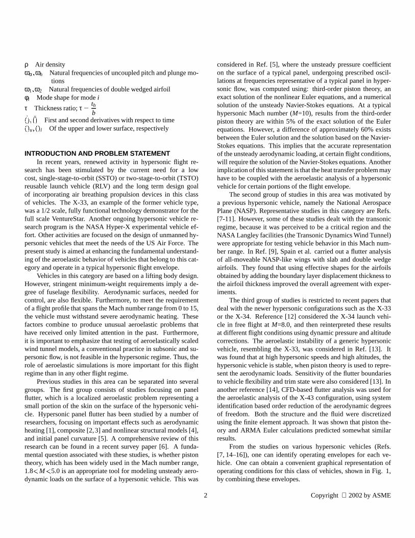
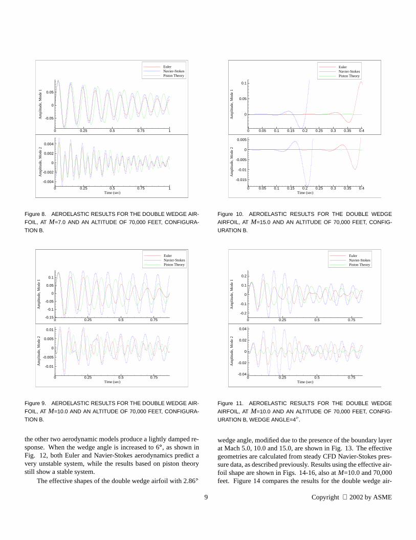
For configuration B, Figs. 8-10 indicate that differences insystem responses from the three aerodynamic models are minorat Mach numbers well below the piston theory flutter boundary,but the differences increase with Mach number. At M � 7 � 0,all three aerodynamic models show comparable responses. Fur-thermore, when the Mach number is increased to M � 10 � 0, theNavier-Stokes response is near critical, while the other two aremore stable. However, Euler and piston theory responses are stillcomparable. When the Mach number is increased to M � 15 � 0,all three aerodynamic models predict unstable responses, withdifferent levels of damping. The increases in differences empha-size the important role of aerodynamic nonlinearities and viscos-ity with increasing Mach numbers.

These results also illustrate that inspection of the aeroelasticresponse curves provides only a partial answer. To better under-stand the differences between aeroelastic results based on pis-ton theory, Euler and Navier-Stokes solutions, actual aeroelasticstability boundaries based on system damping need to be estab-lished.

The effect of increasing the wedge angle (or thickness) ofthe airfoil is depicted in Figs. 11 and 12, at M=10.0 and 70,000feet. For a wedge angle of 4

�, it is shown in Fig. 11 that using

Navier-Stokes aerodynamics produces an unstable system, while


Am

plitu

de,M

ode

1

0 0.25 0.5 0.75 1

-0.05

0

0.05


Time(sec)

Am

plitu

de,M

ode

2

0 0.25 0.5 0.75 1

-0.004

-0.002

0

0.002

0.004



TION B.

Time(sec)

Am

plitu

de,M

ode

2

0 0.25 0.5 0.75

-0.01

-0.005

0

0.005

0.01

Am

plitu

de,M

ode

1

0 0.25 0.5 0.75-0.15

-0.1

-0.05

0

0.05

0.1




TION B.

the other two aerodynamic models produce a lightly damped re-sponse. When the wedge angle is increased to 6

�, as shown in

Fig. 12, both Euler and Navier-Stokes aerodynamics predict avery unstable system, while the results based on piston theorystill show a stable system.

The effective shapes of the double wedge airfoil with 2.86�

Time(sec)

Am

plitu

de,M

ode

2

0 0.05 0.1 0.15 0.2 0.25 0.3 0.35 0.4

-0.015

-0.01

-0.005

0

0.005

Am

plitu

de,M

ode

1

0 0.05 0.1 0.15 0.2 0.25 0.3 0.35 0.4

0

0.05

0.1


Figure 10. AEROELASTIC RESULTS FOR THE DOUBLE WEDGE

AIRFOIL, AT M=15.0 AND AN ALTITUDE OF 70,000 FEET, CONFIG-

URATION B.A

mpl

itude

,Mod

e1

0 0.25 0.5 0.75

-0.2

-0.1

0

0.1

0.2


Time(sec)

Am

plitu

de,M

ode

2

0 0.25 0.5 0.75-0.04

-0.02

0

0.02

0.04



URATION B, WEDGE ANGLE=4�.

wedge angle, modified due to the presence of the boundary layerat Mach 5.0, 10.0 and 15.0, are shown in Fig. 13. The effectivegeometries are calculated from steady CFD Navier-Stokes pres-sure data, as described previously. Results using the effective air-foil shape are shown in Figs. 14-16, also at M=10.0 and 70,000feet. Figure 14 compares the results for the double wedge air-


Time(sec)

Am

plitu

de,M

ode

2

0 0.1 0.2 0.3 0.4 0.5 0.6

-4

-2

0

2

Am

plitu

de,M

ode

1

0 0.1 0.2 0.3 0.4 0.5 0.6-4

-2

0

2

4

6

8




URATION B, WEDGE ANGLE=6�.

x-coordinate (feet)

thic

knes

s(f

eet)

-3 -2 -1 0 1 2 3

-0.25

-0.2

-0.15

-0.1

-0.05

0

0.05

0.1

0.15

0.2

0.25

doublewedgeairfoil, 2.86o

Effectiveshape, Mach 7.0Effectiveshape, Mach 10.0Effectiveshape, Mach 15.0

Figure 13. EFFECTIVE SHAPES OF THE DOUBLE WEDGE AIRFOIL

WITH 2.86�WEDGE ANGLE.

foil with 2.86�

wedge angle (standard geometry), while Fig. 15compares the results for a 4

�wedge angle, and Fig. 16 shows the

results for a 6�wedge angle. In all three cases, the Navier-Stokes

model predicts larger modal amplitudes than piston theory withthe effective shape. Furthermore, at the smallest wedge angle,the piston theory model has a higher level of damping than theNavier-Stokes model. When the wedge angle is increased to 4

�,

the Navier-Stokes model predicts a response with a beat phe-nomenon, therefore it is difficult to identify the degree of damp-ing. However, the piston theory model predicts stable system be-havior. At the 6

�wedge angle, both models predict unstable be-

havior. It should also be noted that at the 6�wedge angle, piston

theory without the effective shape predicted a stable response.

Time(sec)

Am

plitu

de,M

ode

2

0 0.25 0.5 0.75

-0.01

-0.005

0

0.005

0.01

Am

plitu

de,M

ode

1

0 0.25 0.5 0.75-0.15

-0.1

-0.05

0

0.05

0.1

Navier-StokesPT, effectiveshape


AIRFOIL, AT M=10.0 AND AN ALTITUDE OF 70,000 FEET, CON-

FIGURATION B, WEDGE ANGLE=2.86�. COMPARISON OF NAVIER-

STOKES RESULTS WITH EFFECTIVE SHAPE USING PISTON THE-

ORY.

Due to these differences, and limitation of results generated,it is apparent that more study is needed to fully understand thecapability of piston theory with an effective shape in accuratelycapturing viscous effects.

CONCLUSIONSBased on the limited amount of numerical results presented

in this paper, the following conclusions can be stated.

1. The time steps to be used in computational aeroelastic-ity studies are strongly dependent on the unsteady aero-dynamic model used. Using a viscous flow based on theNavier-Stokes equations requires substantially smaller time-step sizes than those used for an Euler solution.

2. Aeroelastic behavior is sensitive to the unsteady aerody-namic model used. For the cases considered, results basedon piston theory are more stable than those from Euler andNavier-Stokes based aerodynamic loads.


Am

plitu

de,M

ode

1

0 0.25 0.5 0.75

-0.2

-0.1

0

0.1

0.2

Navier-StokesPT, effectiveshape

Time(sec)

Am

plitu

de,M

ode

2

0 0.25 0.5 0.75-0.04

-0.02

0

0.02

0.04



URATION B, WEDGE ANGLE=4�. COMPARISON OF NAVIER-STOKES

RESULTS WITH EFFECTIVE SHAPE USING PISTON THEORY.

3. Aeroelastic response results using third order piston theoryand exact Euler solutions are fairly close, and predict similarresponse.

4. Airfoil shapes modified by the presence of a static boundarylayer produce an aeroelastic response that differs substan-tially from that based on the solution of the Navier-Stokesequations.

5. The results presented can be considered to provide a par-tial validation of the CFL3D code for the hypersonic flowregime.

ACKNOWLEDGEMENTThe authors wish to express their gratitude to NASA Lan-

gley Research Center for the CFL3D code and thank Drs. R.Bartels and R. Biedron for their help in using this code. Thisresearch is funded by AFOSR under grant number F49620-01-1-0158 with Dr. D. Mook as program manager.

REFERENCES[1] Xue, D.Y. and Mei, C., “Finite Element Two-Dimensional

Panel Flutter at High Supersonic Speeds and ElevatedTemperature,” AIAA Paper No. 90-0982, Proc. 31stAIAA/ASME/ASCE/AHS/ASC Structures, Structural Dy-namics and Materials Conference, 1990, pp. 1464–1475.

[2] Gray, E.G. and Mei, C., “Large-Amplitude Finite El-ement Flutter Analysis of Composite Panels in Hyper-

Am

plitu

de,M

ode

1

0 0.05 0.1 0.15 0.2 0.25 0.3 0.35 0.4 0.45 0.5 0.55 0.6 0.65-6

-4

-2

0

2

4

6

8

Navier-StokesPt, effectiveshape

Time(sec)

Am

plitu

de,M

ode

2

0 0.05 0.1 0.15 0.2 0.25 0.3 0.35 0.4 0.45 0.5 0.55 0.6 0.65

-1

0

1



URATION B, WEDGE ANGLE=6�. COMPARISON OF NAVIER-STOKES

RESULTS WITH EFFECTIVE SHAPE USING PISTON THEORY.

sonic Flow,” AIAA Paper No. 92-2130, Proc. 33rdAIAA/ASME/ASCE/AHS/ASC Structures, Structural Dy-namics and Materials Conference, Dallas, TX, April 16-171992, pp. 492–512.

[3] Abbas, J.F. and Ibrahim,R.A., “Nonlinear Flutter of Or-thotropic Composite Panel Under Aerodynamic Heating,”AIAA J., Vol. 31, No. 8, No. 8, 1993, pp. 1478–1488.

[4] Bein, T., Friedmann, P., Zhong, X., and Nydick, I., “Hy-personic Flutter of a Curved Shallow Panel with Aero-dynamic Heating,” AIAA Paper No. 93-1318, Proc. 34thAIAA/ASME/ASCE/AHS/ASC Structures, Structural Dy-namics and Materials Conference, La Jolla, CA, April 19-22 1993.

[5] Nydick, I., Friedmann, P.P., and Zhong, X., “HypersonicPanel Flutter Studies on Curved Panels,” AIAA Paper no.95-1485, Proc. 36th AIAA/ASME/ASCE/AHS/ASC Struc-tures, Structural Dynamics and Materials Conference, NewOrleans, LA, April 1995, pp. 2995–3011.

[6] Mei, C., Abdel-Motagly, K., and Chen, R., “Review ofNonlinear Panel Flutter at Supersonic and HypersonicSpeeds,” Applied Mechanics Reviews, 1998.

[7] Ricketts, R., Noll, T., Whitlow, W., and Huttsell,L.,“An Overview of Aeroelasticity Studies for the NationalAerospace Plane,” AIAA Paper No. 93-1313, Proc. 34thAIAA/ASME/ASCE/AHS/ASC Structures, Structural Dy-namics and Materials Conference, La Jolla, CA, April 19-22 1993, pp. 152 – 162.

[8] Scott, R.C. and Pototzky, A.S., “A Method of


Predicting Quasi-Steady Aerodynamics for Flut-ter Analysis of High Speed Vehicles Using SteadyCFD Calculations,” AIAA Paper No. 93-1364,Proc. 34th AIAA/ASME/ASCE/AHS/ASC Struc-tures, Structural Dynamics and Materials Conference, LaJolla, CA, April 19-22 1993, pp. 595–603.

[9] Spain, C., Zeiler, T.A., Bullock, E., and Hodge, J.S., “AFlutter Investigation of All-Moveable NASP-Like Wingsat Hypersonic Speeds,” AIAA Paper No. 93-1315, Proc.34th AIAA/ASME/ASCE/AHS/ ASC Structures, StructuralDynamics and Materials Conference, La Jolla, CA, April19-22 1993.

[10] Spain, C., Zeiler, T.A., Gibbons, M.D., Soistmann, D.L.,Pozefsky, P., DeJesus, R.O., and Brannon,C.P., “Aeroelas-tic Character of a National Aerospace Plane DemonstratorConcept,” Proc. 34th AIAA/ASME/ASCE/AHS/ ASC Struc-tures, Structural Dynamics and Materials Conference, LaJolla, CA, April 19-22 1993, pp. 163–170.

[11] Heeg, J., Zeiler, T., Pototzky, A., Spain, C., and Engelund,W., “Aerothermoelastic Analysis of a NASP Demon-strator Model,” AIAA Paper No. 93-1366, Proc. 34thAIAA/ASME/ASCE/AHS/ ASC Structures, Structural Dy-namics and Materials Conference, La Jolla, CA, April 19-22 1993, pp. 617–627.

[12] Blades, E., Ruth, M., and Fuhrman, D., “Aeroelastic Analy-sis of the X-34 Launch Vehicle,” AIAA Paper No. 99-1352,Proc. 40th AIAA/ASME/ASCE/AHS/ ASC Structures, Struc-tural Dynamics and Materials Conference, St. Louis, MO,1999, pp. 1321–1331.

[13] Nydick, I. and Friedmann, P.P., “Aeroelastic Analy-sis of a Generic Hypersonic Vehicle,” NASA/CP-1999-209136/PT2, Proc. CEAS/AIAA/ICASE/NASA Langley In-ternational Forum on Aeroelasticity and Structural Dynam-ics, Williamsburg, VA, June 22-25 1999, pp. 777–810.

[14] Gupta, K.K., Voelker, L.S., Bach, C., Doyle, T., andHahn, E., “CFD-Based Aeroelastic Analysis of the X-43Hypersonic Flight Vehicle,” AIAA Paper No. 2001-0712,39th Aerospace Sciences Meeting & Exhibit, 2001.

[15] Berry, S.A., Horvath, T.J., Hollis, B.R., Thompson, R.A.,and Hamilton, H.H., “X-33 Hypersonic Boundary LayerTransition,” AIAA Paper No. 99-3560, 33rd AIAA Thermo-physics Conference, Norfolk, VA, June 28 - July 1 1999.

[16] Riley, C.J., Kleb, W.L., and Alter, S.J., “AeroheatingPredictions for X-34 Using An Inviscid-Boundary LayerMethod,” AIAA 98-0880, 36th Aerospace Sciences Meet-ing & Exhibit, Reno, NV, January 1998.

[17] Thuruthimattam, B.J., Friedmann, P.P., McNamara, J.J.,and Powell, K.G., “Aeroelasticity of a Generic Hyper-sonic Vehicle,” AIAA Paper No. 2002-1209, Proc. 43rdAIAA/ASME/ASCE/AHS Structures, Structural Dynamicsand Materials Conference, Denver, CO, April 2002.

[18] Bousman, W.G. and Winkler, D.J., “Application of the

Moving-Block Analysis,” AIAA 81-0653, Proceedings ofthe AIAA Dynamics Specialist Conference, Atlanta, GA,April 1981, pp. 755–763.

[19] Krist, S.L., Biedron, R.T., and Rumsey, C.L., “CFL3DUser’s Manual (Version 5.0),” NASA, TM 1998-208444,1997.

[20] Robinson, B.A., Batina, J.T., and Yang, H.T., “Aeroelas-tic Analysis of Wings Using the Euler Equations with aDeforming Mesh,” Journal of Aircraft, Vol. 28, November1991, pp. 778–788.

[21] Cunningham, H.J., Batina, J.T., and Bennett, R.M., “Mod-ern Wing Flutter Analysis by Computational Fluid Dy-namic Methods,” Journal of Aircraft, Vol. 25, No. 10,No. 10, 1989, pp. 962–968.

[22] Lee-Rausch, E.M. and Batina, J.T., “Wing FlutterBoundary Prediction Using Unsteady Euler Aerody-namic Method,” AIAA Paper No. 93-1422, Proc. 34thAIAA/ASME/ASCE/AHS Structures, Structural Dynamicsand Materials Conference, 1993, pp. 1019–1029.

[23] Lee-Rausch, E.M. and Batina, J.T., “Calculation ofAGARD Wing 445.6 Flutter Using Navier-Stokes Aerody-namics,” AIAA Paper No. 93-3476, Proc. AIAA 11th Ap-plied Aerodynamics Conference, Hampton, VA, August 9-11 1993.

[24] Ashley, H. and Zartarian, G., “Piston Theory - A New Aero-dynamic Tool for the Aeroelastician,” Journal of the Aero-nautical Sciences, Vol. 23, No. 12, No. 12, 1956, pp. 1109–1118.

[25] Lighthill, M.J., “Oscillating Airfoils at High Mach Num-bers,” Journal of the Aeronautical Sciences, Vol. 20, No. 6,June 1953.

[26] Anderson, J.D., Hypersonic and High Temperature GasDynamics, New York, McGraw-Hill, 1989.


paper2col - Semantic Scholar · Develop an aeroelastic analysis for a double wedge airfoil in...

Documents

Transcript of paper2col - Semantic Scholar · Develop an aeroelastic analysis for a double wedge airfoil in...