AIR FORCE INSTITUTE OF TECHNOLOGY · and hypersonic airfoil designs and materials sponsored by...
114
ExFiT Flight Design and Structural Modeling for FalconLAUNCH VIII Sounding Rocket THESIS Michael J. Vinacco, Second Lieutenant, USAF AFIT/GAE/ENY/10-M27 DEPARTMENT OF THE AIR FORCE AIR UNIVERSITY AIR FORCE INSTITUTE OF TECHNOLOGY Wright-Patterson Air Force Base, Ohio APPROVED FOR PUBLIC RELEASE; DISTRIBUTION UNLIMITED
Transcript of AIR FORCE INSTITUTE OF TECHNOLOGY · and hypersonic airfoil designs and materials sponsored by...

ExFiT Flight Design and Structural Modeling for
FalconLAUNCH VIII Sounding Rocket
THESIS
Michael J. Vinacco, Second Lieutenant, USAF
AFIT/GAE/ENY/10-M27
DEPARTMENT OF THE AIR FORCEAIR UNIVERSITY
AIR FORCE INSTITUTE OF TECHNOLOGY
Wright-Patterson Air Force Base, Ohio
APPROVED FOR PUBLIC RELEASE; DISTRIBUTION UNLIMITED

The views expressed in this thesis are those of the author and do not reflect the official
policy or position of the United States Air Force, Department of Defense,
or the United States Government.
This material is declared a work of the U.S. Government and is not subject
to copyright protection in the United States.

AFIT/GAE/ENY/10-M27
ExFiT Flight Design and Structural Modeling for FalconLAUNCH
VIII Sounding Rocket
THESIS
Presented to the Faculty
Department of Aeronautics and Astronautics
Graduate School of Engineering and Management
Air Force Institute of Technology
Air University
Air Education and Training Command
In Partial Fulfillment of the Requirements for the
Degree of Master of Science in Aeronautical Engineering
Michael J. Vinacco, B.S.
Second Lieutenant, USAF
March, 2010
APPROVED FOR PUBLIC RELEASE; DISTRIBUTION UNLIMITED

AFIT/GAE/ENY/10-M27
Abstract
This research effort furthers the Air Force’s study of reusable launch vehicles and
hypersonic airfoils by conducting a hypersonic flight test using the US Air Force Academy’s
FalconLAUNCH VIII sounding rocket. In this study, two experimental fin tips were designed
and attached to the sounding rocket in place of two stabilizer fins in order to collect data
throughout the rocket’s hypersonic flight profile. The desire to research, study, and test
experimental fin tips was driven by the Air Force Research Laboratory’s Future responsive
Access to Space Technologies (FAST) program and their desire to include vertical stabilizers
on the wing tips of reusable launch vehicles (RLVs). In this research study, finite element
models of the experimental fin tips were developed and used to predict the flight data
collected by the strain and temperature gages attached to the test specimen. The results
of these flight prediction tests showed that the test specimen will undergo the greatest
deflection and strain during the acceleration of the rocket. Maximum deflection and strain
gage readings were obtained at a speed of Mach 2.5 at an altitude of 9k feet. Ultimately,
the payload will undergo a maximum deflection of 0.6 inches at the fin tip and a maximum
strain gage reading of 0.00122 on the main wing section of the payload.
iv

Acknowledgements
First off, I’d like to thank God for the countless blessings he continues to bestow upon
me and my family. I am reminded time and time again how very lucky I am.
Second, I’d like to thank my beautiful wife for her constant love and understanding
while I spent countless hours working, studying, and complaining here at AFIT. You remain
my constant source of happiness and I just can’t thank you enough. I love you.
Next, I’d like to thank the rest of my family. You guys have seen me through a lot
of hard times throughout the past few years. I love you all so much and thank you for the
support you have given me.
To my committee, your constant help and direction with this paper proved absolutely
vital. Thanks for the guidance and understanding you have given me for the past year and
a half.
Air Force Academy professors and FalconLAUNCH VIII design team, thank you for
including me in your project and for constantly working with me throughout the year. I’m
excited for the upcoming launch, and greatful that I could be of assitance!
Now, I have to thank all the guys in the Lair of Despair. You’ve somehow made this
painful process slightly enjoyable. Thanks for the Qdoba runs and the Foosball tournaments;
it kept me sane.
Furthermore, I’d like to thank my best-man from the Tribe of W&M. Thanks for all
the Halo and Resident Evil gaming sessions as well as putting up with my complaining and
crazy cleaning habits before I got married. Enjoy your time in China my friend, but come
home soon.
Finally, I want to give a shout-out to all my Brother Rats from the Mother-I. You
guys have and will always be there to help me out. I love you guys and I want you to know
I’ll always have your backs. Rah Virginia Mil and the Class of 2008.
Michael J. Vinacco
v

Table of Contents
Page
Abstract . . . . . . . . . . . . . . . . . . . . . . . . . . . . . . . . . . . . . . . . . iv
Acknowledgements . . . . . . . . . . . . . . . . . . . . . . . . . . . . . . . . . . . v
Nomenclature . . . . . . . . . . . . . . . . . . . . . . . . . . . . . . . . . . . . . . ix
List of Tables . . . . . . . . . . . . . . . . . . . . . . . . . . . . . . . . . . . . . . x
List of Figures . . . . . . . . . . . . . . . . . . . . . . . . . . . . . . . . . . . . . xi
I. Introduction . . . . . . . . . . . . . . . . . . . . . . . . . . . . . . . . . . . . 1
1.1 Purpose of Research . . . . . . . . . . . . . . . . . . . . . . . . . . . 1
1.2 Research Approach . . . . . . . . . . . . . . . . . . . . . . . . . . . . 2
1.3 Thesis Overview . . . . . . . . . . . . . . . . . . . . . . . . . . . . . 5
II. Literature Review . . . . . . . . . . . . . . . . . . . . . . . . . . . . . . . . . 7
2.1 Chapter Overview . . . . . . . . . . . . . . . . . . . . . . . . . . . . 7
2.2 The Dyna-Soar X-20 Program (1957-1963) . . . . . . . . . . . . . . . 7
2.3 NASAs Lifting Body Program and the HL-10 (1958-1970) . . . . . . 10
2.4 DARPAs HTV-3X Blackswift . . . . . . . . . . . . . . . . . . . . . . 12
2.5 HIFiRE Hypersonic Research Program . . . . . . . . . . . . . . . . . 14
2.6 Current Research under the FAST program . . . . . . . . . . . . . . 17
2.7 US Air Force Academy Partnership with AFIT . . . . . . . . . . . . 18
2.8 Summary . . . . . . . . . . . . . . . . . . . . . . . . . . . . . . . . . 21
III. Methodology . . . . . . . . . . . . . . . . . . . . . . . . . . . . . . . . . . . . 24
3.1 Chapter Overview . . . . . . . . . . . . . . . . . . . . . . . . . . . . 24
3.2 Software used in this research . . . . . . . . . . . . . . . . . . . . . . 24
vi

Page
3.2.1 FEMAP v9.31 . . . . . . . . . . . . . . . . . . . . . . 24
3.2.2 AeroFinSim v4.0 . . . . . . . . . . . . . . . . . . . . . 26
3.3 Design Criteria for FalconLAUNCH VIII Experiment . . . . . . . . . 27
3.3.1 Experiment Geometry Selection . . . . . . . . . . . . . 27
3.3.2 Experimental Size and Location . . . . . . . . . . . . . 28
3.3.3 Material Selection for the Experiment . . . . . . . . . 29
3.3.4 Sensor Selection and Placement . . . . . . . . . . . . . 33
3.4 Flutter Analysis . . . . . . . . . . . . . . . . . . . . . . . . . . . . . 34
3.5 FEM Progression and Initial Analysis . . . . . . . . . . . . . . . . . 35
3.5.1 Flat Plate Models . . . . . . . . . . . . . . . . . . . . 35
3.5.2 Meshing Complex Geometries . . . . . . . . . . . . . . 36
3.5.3 Full Wing Models . . . . . . . . . . . . . . . . . . . . 39
3.5.4 Modal Analysis of FE Models . . . . . . . . . . . . . . 43
3.5.5 Material Property Comparison . . . . . . . . . . . . . 43
3.5.6 Mesh Refinement . . . . . . . . . . . . . . . . . . . . . 45
3.6 Ping Test Validation . . . . . . . . . . . . . . . . . . . . . . . . . . . 46
3.7 Flight Prediction using FEMs . . . . . . . . . . . . . . . . . . . . . . 48
3.7.1 FEM Modifications . . . . . . . . . . . . . . . . . . . . 48
3.7.2 Flight Profile Test Points . . . . . . . . . . . . . . . . 49
3.7.3 CFD Analysis . . . . . . . . . . . . . . . . . . . . . . . 50
3.7.4 Heating Effect . . . . . . . . . . . . . . . . . . . . . . 52
3.8 Chapter Summary . . . . . . . . . . . . . . . . . . . . . . . . . . . . 53
IV. Results for FalconLAUNCH VIII Flight Prediction Experiments and Future
Models . . . . . . . . . . . . . . . . . . . . . . . . . . . . . . . . . . . . . . . 54
4.1 Chapter Overview . . . . . . . . . . . . . . . . . . . . . . . . . . . . 54
4.2 AeroFinSim Results . . . . . . . . . . . . . . . . . . . . . . . . . . . 54
4.3 Ping Test Results and Comparisons . . . . . . . . . . . . . . . . . . 56
vii

Page
4.4 Flight Prediction Test Loading Setup . . . . . . . . . . . . . . . . . . 60
4.5 Flight Prediction Results . . . . . . . . . . . . . . . . . . . . . . . . 62
4.5.1 CFD Results . . . . . . . . . . . . . . . . . . . . . . . 62
4.5.2 Final Loading Configurations . . . . . . . . . . . . . . 65
4.5.3 Strain Gage Predictions . . . . . . . . . . . . . . . . . 65
4.5.4 Test Specimen Deflections . . . . . . . . . . . . . . . . 69
4.6 Heating Analysis Results . . . . . . . . . . . . . . . . . . . . . . . . 72
4.7 Carbon-Fiber Composite Study . . . . . . . . . . . . . . . . . . . . . 74
4.7.1 Material Property Changes . . . . . . . . . . . . . . . 74
4.7.2 Modal Analysis . . . . . . . . . . . . . . . . . . . . . . 76
4.7.3 Strain Gage Predictions . . . . . . . . . . . . . . . . . 78
4.7.4 Test Specimen Deflections . . . . . . . . . . . . . . . . 82
4.8 Chapter Summary . . . . . . . . . . . . . . . . . . . . . . . . . . . . 84
V. Conclusions and Recommendations for Future Work . . . . . . . . . . . . . . 88
5.1 Chapter Overview . . . . . . . . . . . . . . . . . . . . . . . . . . . . 88
5.2 Conclusions . . . . . . . . . . . . . . . . . . . . . . . . . . . . . . . . 88
5.3 Recommendations for Future FalconLAUNCH and AFRL FAST Work 90
5.3.1 Future Flutter Prediction Tests . . . . . . . . . . . . . 90
5.3.2 Rocket Vibration and Dynamic Loading for FEMs . . 91
5.3.3 Validating and Tuning the FEMs Created for Flight
Prediction . . . . . . . . . . . . . . . . . . . . . . . . . 92
5.3.4 Sensor Locations for Future Experiments . . . . . . . 93
5.3.5 Material Selection and Heating Profile Studies . . . . . 95
5.3.6 Shape and Location of Next Year’s Experiment . . . . 96
5.3.7 Scaling Results to a Full-Size Vehicle . . . . . . . . . . 97
Bibliography . . . . . . . . . . . . . . . . . . . . . . . . . . . . . . . . . . . . . . 98
Vita . . . . . . . . . . . . . . . . . . . . . . . . . . . . . . . . . . . . . . . . . . . 100
viii
Nomenclature
Abbreviations
AFIT Air Force Institute of Technology
AFRL/RB Air Force Research Laboratory Air Vehicles Directorate
CFD Computational Fluid Dynamics
CRADA Cooperative Research and Development Agreement
DARPA Defense Advanced Research Project Agency
DSTO Australian Defence Science and Technology Organisation
ExFiT Experimental Fin Tip - AFIT Program
FALCON Force Application and Launch from CONUS
FAST Future Responsive Access to Space Technologies
FE Finite Element
FEMs Finite Element Models
HCV Hypersonic Cruise Vehicle
HIFiRE Hypersonic International Flight Research and Experimentation
HTVs Hypersonic Technology Vehicles
HWS Hypersonic Weapons System
ICBMs Intercontinental Ballistic Missiles
NACA National Advisory Committee for Aeronautics
NASA National Aeronautics and Space Administration
RBS Reusable Booster System
RFS Reference Flight System
RLVs Reusable Launch Vehicles
RTLS Return to Launch Site
SBIR Small Business Innovative Research
SLV Small Launch Vehicle
ix

List of TablesTable Page
1. First three natural frequencies(Hz) of FE models using Al6061-T6 . . 43
2. Natural Frequencies (Hz) of Different Materials . . . . . . . . . . . . . 45
3. Mesh Refinement Study . . . . . . . . . . . . . . . . . . . . . . . . . . 45
4. Flight Profile Data Points for FE Testing . . . . . . . . . . . . . . . . 51
5. Young’s Modulus Variation for Heating Effect . . . . . . . . . . . . . 53
6. Dimensions of Test Specimen Sections Used in AeroFinSim (in.) . . . 54
7. AeroFinSim Flutter Results . . . . . . . . . . . . . . . . . . . . . . . . 55
8. Natural Frequency Comparison (Hz) . . . . . . . . . . . . . . . . . . . 60
9. 5k, Mach 1.0 Test Configuration . . . . . . . . . . . . . . . . . . . . . 63
10. 9k, Mach 2.5 Test Configuration . . . . . . . . . . . . . . . . . . . . . 63
11. 30k, Mach 4.5 Test Configuration . . . . . . . . . . . . . . . . . . . . 63
12. 60k, Mach 2.5 Test Configuration . . . . . . . . . . . . . . . . . . . . 64
13. 100k, Mach 1.0 Test Configuration . . . . . . . . . . . . . . . . . . . . 64
14. Aluminum Model Strain Readings . . . . . . . . . . . . . . . . . . . . 67
15. Aluminum Model Deflection Predictions . . . . . . . . . . . . . . . . . 70
16. First Three Natural Frequencies (Hz) of Aluminum Model with Re-
duced Young’s Modulus due to Heating . . . . . . . . . . . . . . . . . 72
17. Carbon-Fiber Modal Analysis . . . . . . . . . . . . . . . . . . . . . . 76
18. Carbon-Fiber Model Strain Readings . . . . . . . . . . . . . . . . . . 78
19. Carbon-Fiber Model Deflection Predictions . . . . . . . . . . . . . . . 83
x
List of FiguresFigure Page
1. Potential FAST Reusable Booster System with an Upper Stage [1] . . 2
2. FAST Reference Flight System (RFS)[1] . . . . . . . . . . . . . . . . 3
3. Experimental Fin Tip for FalconLAUNCH VIII . . . . . . . . . . . . 3
4. Design of FalconLAUNCH VIII Sounding Rocket with ExFiT attached 4
5. Model of ExFiT Sensor Placement for FalconLAUNCH VIII . . . . . 5
6. Dyna-Soar X-20 Hypersonic Vehicle Mock Up[2] . . . . . . . . . . . . 8
7. Dyna-Soar X-20 Hypersonic Vehicle with Booster[3] . . . . . . . . . . 8
8. NASA M2-F1 Vehicle[4] . . . . . . . . . . . . . . . . . . . . . . . . . 11
9. NASA HL-10 Lifting Body Vehicle[5] . . . . . . . . . . . . . . . . . . 11
10. Model of the HTV-3X Blackswift[6] . . . . . . . . . . . . . . . . . . . 13
11. Artist Rendering of the HTV-3X Blackswift[7] . . . . . . . . . . . . . 14
12. Picture of the HIFiRE-0 Launch in May 2009 [8] . . . . . . . . . . . 16
13. XCOR Aerospace Lynx Vehicle Model[9] . . . . . . . . . . . . . . . . 18
14. Experimental Fin Tip attached to FalconLAUNCH VII (2008-2009) . 20
15. Flight Profile of FalconLAUNCH VII (2008-2009) . . . . . . . . . . . 21
16. Screenshot of FEMAP v9.31 Interface . . . . . . . . . . . . . . . . . . 25
17. Screenshot of AeroFinSim v4.0 Results . . . . . . . . . . . . . . . . . 27
18. Casting Test Specimen Top View . . . . . . . . . . . . . . . . . . . . 31
19. Casting Test Specimen Angled View . . . . . . . . . . . . . . . . . . . 32
20. Sensor Gages on Experiment . . . . . . . . . . . . . . . . . . . . . . . 34
21. First Flat Plate Model . . . . . . . . . . . . . . . . . . . . . . . . . . 36
22. Second Flat Plate Model . . . . . . . . . . . . . . . . . . . . . . . . . 37
23. Surface Hole . . . . . . . . . . . . . . . . . . . . . . . . . . . . . . . . 38
24. New Surface Node . . . . . . . . . . . . . . . . . . . . . . . . . . . . . 38
25. New Fixed Surface - No Hole . . . . . . . . . . . . . . . . . . . . . . . 39
xi

Figure Page
26. First Full Wing Model . . . . . . . . . . . . . . . . . . . . . . . . . . 40
27. Final Full Wing Model . . . . . . . . . . . . . . . . . . . . . . . . . . 40
28. Additional View of Model . . . . . . . . . . . . . . . . . . . . . . . . . 41
29. Mesh Refinement Model . . . . . . . . . . . . . . . . . . . . . . . . . 42
30. Al A357-T6 Property Card Creation . . . . . . . . . . . . . . . . . . . 44
31. Ping Test Experimental Setup . . . . . . . . . . . . . . . . . . . . . . 47
32. FEM Slicing Progression from Top Left to Bottom Right . . . . . . . 50
33. Flight Profile for FalconLAUNCH VIII . . . . . . . . . . . . . . . . . 51
34. AeroFinSim Flutter Results . . . . . . . . . . . . . . . . . . . . . . . . 56
35. Results from 1st Ping test . . . . . . . . . . . . . . . . . . . . . . . . 57
36. Results from 2nd Ping test . . . . . . . . . . . . . . . . . . . . . . . . 58
37. Results from 3rd Ping test . . . . . . . . . . . . . . . . . . . . . . . . 59
38. Point Created in Surface Centroid . . . . . . . . . . . . . . . . . . . . 61
39. Final Loading Configuration for Flight Prediction Tests . . . . . . . . 65
40. Strain Contours for Flight Test Points . . . . . . . . . . . . . . . . . . 66
41. Plot of Aluminum Model Strain Results . . . . . . . . . . . . . . . . . 68
42. Deflection Contours for Flight Test Points . . . . . . . . . . . . . . . 69
43. Plot of Aluminum Model Deflection Results . . . . . . . . . . . . . . 71
44. AGP370-5H Carbon Fiber Property Card . . . . . . . . . . . . . . . . 75
45. Strain Contours for Carbon-Fiber Flight Test Points . . . . . . . . . . 79
46. Plot of Carbon-Fiber Model Strain Results . . . . . . . . . . . . . . . 81
47. Deflection Contours for Carbon-Fiber Flight Test Points . . . . . . . 82
48. Plot of Carbon-Fiber Model Deflection Results . . . . . . . . . . . . . 84
49. First Three Natural Mode Shapes of the FEM . . . . . . . . . . . . . 94
50. Location of Future Strain Gage Placement . . . . . . . . . . . . . . . 95
xii

ExFiT Flight Design and Structural Modeling for FalconLAUNCH
VIII Sounding Rocket
I. Introduction
The intent of this research is to further the Air Force’s study of reusable launch vehicles
and hypersonic airfoil designs and materials sponsored by ARFL/RB in conjunction with
the US Air Force Academy’s FalconLAUNCH program. In order to accomplish this task, two
seperate experimental fin tips were designed to fly on the FalconLAUNCH VIII sounding
rocket in order to collect strain gage and temperature flight data during the supersonic and
low hypersonic flight regime experienced by the rocket. The vertically mounted wing tips in
this experiment are scaled down airfoils resembling current AFRL/RB concept vehicles. In
accordance with this goal, several computational finite element models (FEMs) were created
and validated in order to aid in flight data prediction along with laying the ground work for
future research and study in the field of experimental fin tip design and behavior.
1.1 Purpose of Research
Presently, AFRL/RB, through its FAST program, is studying a Reusable Booster
System (RBS) to meet the Air Force’s future space launch requirements. Expanding on
the requirements for the RBS, the Air Force wants a platform that can be launched tens
of times a year with the most cost effective reusable first stage and an expendable upper
stage. Furthermore, AFRL/RB’s concept calls for seperation anywhere from 80-100 kft with
speeds approaching Mach 5.0 [1]. An example of a potential RBS is shown in Figure 1 with
an upper stage mounted on top.
The Air Force’s RBS concept incorporates the usage of wing tip mounted vertical
stabilizers in its design. That being the case, it will be necessary to design the wing tips
so that they are capable of withstanding the hypersonic flight regime they will experience.
The RBS will use the verical fins for a variety of reasons. First, the vertical wing tips
1

Figure 1 Potential FAST Reusable Booster System with an Upper Stage [1]
have more exposure to the freestream at the supersonic and hypersonic speeds experienced
in flight. In this arrangement, the fuselage will not shield the vertical stabilizers during
reentry. Secondly, the vertically-mounted wing tips will reduce the amount of structural
support required in the back of the vehicle and will allow much easier access to critical
engine components located in the aft section for maintenance between flights. This fact
alone will serve to increase the operability of the aircraft. Lastly, this design will provide
for easier upper stage integration on the leeward side of the vehicle [1].
For these reasons, the Experimental Fin Tip (ExFiT) program has been established
to conduct further research on the vertically mounted wing tips incorporated into the RBS.
This body of work intends to set up an experiment designed to collect data on geometrically-
scaled veritcally mounted wing tips throughout its intended supersonic and low hypersonic
flight regime as well as develop the necessary computer models to replicate the data and
give insight into the behavior and performance of the full-scale concept vehicle.
1.2 Research Approach
In order to perform a study on the experimental wing tips that would be relevant to
the FAST concept vehicle shown in Figure 2, a geometry was selected that closely resembles
this configuration.
The wing and geometry used for this study resembles the FAST vehicle in that they
both contain the double-delta airfoil shape with vertical stabilizers mounted on each wing
2

Figure 2 FAST Reference Flight System (RFS)[1]
Figure 3 Experimental Fin Tip for FalconLAUNCH VIII
tip. However, in this research study the geometry selected will be scaled down by a factor
of 10 and attached to a sounding rocket in order to obtain the desired supersonic and low
hypersonic flight regime. Figure 3 shows the dimensions and configuration of the experiment
to be attached to US Air Force Academy’s FalconLAUNCH VIII sounding rocket in order
to collect data that would closely resemble the FAST vehicle’s intended flight profile.
As an overview, the US Air Force Academy’s FalconLAUNCH program is a senior
design project whereby the cadets design, build and fly a sounding rocket over the course of
one academic year. For the 2010 flight, two of the rocket’s stablizer fins have been replaced
with the ExFiT fins cast from Aluminum A357-T6 material. Shown in Figure 4 is the
intended design of the FalconLAUNCH VIII sounding rocket reflecting the experimental
setup of academic year 2009-2010.
3

Figure 4 Design of FalconLAUNCH VIII Sounding Rocket with ExFiT attached
In order to study the behavior of the ExFiT fins on the rocket during its flight, several
different informational gages have been attached to the experiment in order to collect flight
data while the data will be streamed to the ground during the actual flight. Figure 5
represents the two strain gages and two temperature gages attached to the main wing and
wing-tip portions of the experiment. Once flown, the data collected by the rocket can then
be compared to analytical models.
In addition to designing flight data collection, several finite element models have also
been created in this study. These models advance through various stages of complexity
and accuracy and culminate with a final model that very closely resembles the flight-ready
experiment. These models have been validated through mesh refinement studies, material
property adjustments, and a laser-vibrometer ping test of the flight-ready ExFiT fin itself.
The purpose behind these validated finite element models will be to continue ExFiT research
with the hopes of predicting flight behavior for experimental launches in future years and
full-scale hypersonic and reusable launch vehicle airfoils.
4

Figure 5 Model of ExFiT Sensor Placement for FalconLAUNCH VIII
1.3 Thesis Overview
There are many facets to this research project and experiment. In order to provide a
logical progression of ideas and work, the following outline can be used as a quick reference
for each topic discussed.
1. Chapter 1: Introduction provided the background of the work on experimental fin tips
as well as the purpose and approach of the research conducted.
2. Chapter 2: The Literature Review will highlight the Air Force’s continued interest
in hypersonic flight as well as discussing the progression of work related to this topic
culminating in the present experiment with the ExFiT program.
3. Chapter 3: The Methodology section will discuss in detail the specifics of all computer
programs used, the details of the current experiment, the progression of finite element
models, and laser vibrometer testing.
4. Chapter 4: This chapter will discuss the results of the finite element models, laser
vibrometer test, and deflection results from the validated models for the current
experiment.
5. Chapter 5: This chapter will outline in detail the recommendations for the continued
work in the ExFiT program in conjunction with the US Air Force Academy and the
5

necessary changes to be made in succeeding years. It will also serve as a conclusions
chapter and will summarize the body of work as well as discuss the overall success of
the program.
6

II. Literature Review
2.1 Chapter Overview
Hypersonic research and development has been at the forefront of past and present
experiments conducted by the Air Force since its inception. Though its goals have changed
throughout the years, it is important to take note of the work conducted in this field up to
this point in order to further understand the full implications of the study at hand. This
chapter will serve as a brief chronological look at hypersonic research projects conducted
by the Air Force, the National Aeronautics and Space Administration (NASA), the Defense
Advance Research Projects Agency (DARPA), and the Hypersonic International Flight
Research and Experimentation (HIFiRE) program throughout the years and ultimately
concluding with the current work on the ExFiT program in conjunction with the the US
Air Force Academy supported by the AFRL/RB FAST program.
2.2 The Dyna-Soar X-20 Program (1957-1963)
The Dyna-Soar boost-glider program was conceived in 1957 as a hypersonic test and
flight vehicle capable of performing a variety of missions. Developed by the Air Force,
the Dyna-Soar was designed to be a hypersonic weapon system flying at an altitude of
90 km while performing its role as manned, hypersonic, global, strategic bombardment
and reconnaissance system [10]. The purpose behind this weapon system was to allow
for global bombing and reconnaissance with greater accuracy and precision then current
intercontinental ballistic missiles (ICBMs). The X-20 would allow for targeting of not only
far stationary but also moving targets with the option to abort at any stage of attack.
Although the X-20 was never actually completed, several mock-ups and artist renderings
had been created to reflect the final design specifications to be incorporated into the final
vehicle. Figures 6 and 7 below reflect the final designs of the X-20.
In addition to its role as a global strike and recon vehicle, the X-20 would also serve a
variety of other purposes. As for its ability to perform experimental tests, the X-20 would
allow for tests of complete missions systems in possible future reconnaissance programs and
other military subsystems while operating in its hypersonic flight regime[10]. The X-20 was
7

Figure 6 Dyna-Soar X-20 Hypersonic Vehicle Mock Up[2]
Figure 7 Dyna-Soar X-20 Hypersonic Vehicle with Booster[3]
8

also very cost-effective in that the vehicle could control its re-entry and glide to its final
destination, whereby the components could be examined and even reused, very similar to
the FAST RBS. Similarly, the production of the X-20 would lend itself to the future study
of hypersonic maneuvering and re-entry spacecraft. In his letter to Secretary of Defense
Robert S. McNamara, assistant secretary for research and development for Major General
Osmond Ritland of the Ballistic Missile Division B. McMillan summarized the importance
of the X-20:
The existing X-20 program will provide techniques for manned maneuverable re-entry and recovery, with the ability to initiate recovery at will, to land at a pre-selectedbase, to recover self-contained payloads for immediate examination and reuse, and torefurbish and reuse the spacecraft itself; all of which are essential to an economicand militarily sound space posture...The reconnaissance mission area offers the mostlikely prospects for operational use of the growth version of the X-20, due to the X-20’s operationally desirable de-orbit, re-entry, and landing characteristics. The flightoptions afforded the pilot by the great lateral range of the X-20 type craft enhances theprobability of mission success during peace time by reducing dependence upon weatherand upon reaching a fixed safe landing spot [like the Gemini capsule required]...Duringwar time the ability to terminate a flight quickly in order to minimize on-orbit exposureto enemy actions and the ability to maneuver to a base with a preferred security,survival, or command posture could be of inestimable value[11].
Sadly, the X-20 was cancelled at McNamara’s bequest in 1963 before completion. He
offered the following somewhat inaccurate statement as his reasons:
The X-20 [Dyna-Soar] was not contemplated as a weapon system or even as aprototype of a weapon system...it was a narrowly defined program, limited primarilyto developing the techniques of controlled re-entry at a time when the broader questionof ‘Do we need to operate in near-earth orbit?’ has not yet been answered...I don’tthink we should start out on a billion dollar program until we lay down very clearlywhat we will do with the product, if and when it proves successful[12].
Although its goals of becoming an operational hypersonic weapons system were never
fully attained, the X-20 was still able to lay the ground work for much of the hypersonic
research continuing today, to include re-usable entry vehicles like FAST’s RSB.
9

2.3 NASAs Lifting Body Program and the HL-10 (1958-1970)
Looking at other venues, the National Advisory Committee for Aeronautics (NACA)
envisioned a lifting body approach to reentry with a horizontal landing in the early 1950s
much like the concept behind FASTs RBS. Basically, a lifting body generates the required
aerodynamic lift necessary for flight from the shape of the craft rather than the use of wings
attached to the body.
From the work of two engineers, H. Julian “Harvey” Allen and Alfred Eggers, NACA
deduced that blunting the nose of a body would better dissipate the energy due to reentry
by means of the large shock generated in front of the nose rather than the shock developed
off a sharp nose which would absorb more heat energy. Ultimately, they concluded that a
blunt-nosed vehicle had a higher chance of survivability than did a sharp nosed vehicle due
to the high heating conditions of reentry. From these simple conclusions came the birth
of NASA’s lifting body program established shortly after the demise of NACA due to the
National Aeronautics and Space Act in October of 1958[13].
In 1963, the first lifting body flight test was conducted with NASA’s M2-F1, nick-
named “the flying bathtub” shown in Figure 8. After achieving some initial success, the
designs of the M2-F1, and later M2-F2, led to the final lifting body geometry tested, the
HL-10, depicted in Figure 9.
The HL-10 was NASA’s final test vehicle for a lifting body reentry vehicle. Flight
tests conducted with this vehicle yielded great results and culminated in a maximum speed
test at Mach 1.86 on February 18, 1970. Although no hypersonic flight tests were ever
conducted, these low supersonic tests were able to prove exactly what NASA scientists
and engineers wanted. Conclusively, this program proved that a lifting body can execute
steep, high-energy, horizontal landings that would later be incorporated into the founding
research of NASAs Space Shuttle. Many of the concepts proved in this program indicated
that FASTs RBS is very plausible, and with actual hypersonic testing, the RBS can become
an operationally effective vehicle.
10

Figure 8 NASA M2-F1 Vehicle[4]
Figure 9 NASA HL-10 Lifting Body Vehicle[5]
11

2.4 DARPAs HTV-3X Blackswift
Jumping forward to the new millenium, the Air Force has once again focused its
attention to a hypersonic cruise weapons platform. In conjunction with DARPA, the
Air Force funded the Force Application and Launch from CONUS (FALCON) program
to develop a way for the Air Force to meet its needs.
In a 2003 publication from DARPA, the following statement summarized the goals for
the joint DARPA/Air Force FALCON program:
The goal of the joint DARPA/Air Force FALCON program is to develop andvalidate, in-flight, technologies that will enable both a near-term and far-term ca-pability to execute time-critical, prompt global reach missions while at the sametime, demonstrating affordable and responsive space lift...while also enabling futuredevelopment of a reusable Hypersonic Cruise Vehicle (HCV) for the far-term[14].
Fueled by the military engagements in Bosnia, Afghanistan, and Iraq, the Air Force
has realized a need to be able to engage and strike time-critical, high value, hard and
deeply-buried targets. Furthermore, the U.S. Strategic Command has realized that it would
be politically advantageous to enable global strike technology from inside the continental
U.S. or alternative U.S. basing within minutes or hours from launch[14].
Broken into three phases, the FALCON program was defined as follows. Phase 1:
A systems definition phase whereby research into a Small Launch Vehicle (SLV) and a
Hypersonic Weapons System (HWS) was conceptually designed, planned, and developed.
Phase 2: A design and development phase whereby the SLV would have been demonstrated
and flown, and the HWS would have been further developed and designed. Phase 3: A
weapon systems demonstration whereby contractors would have conducted flight tests of
the HCV[14].
In its outlines, the developed HCV would be capable of taking off from a conventional
runway, striking targets up to 9000 nautical miles away in less than two hours, and carrying
up to 12000 pounds of payload of either cruise missiles, small diameter bombs, or other
unmanned air vehicles[14].
In order to address the feasability of hypersonic flight and reusability, the FALCON
program developed a series of hypersonic technology vehicles (HTVs) to demonstrate the
12

technological advances required to fulfill its goals. The first vehicle produced in this line
of work was the HTV-1 developed by Lockheed Martin Aeronautics Corporation. This
vehicle was designed to test materials and fabrication challenges involved with the vehicle.
Through various ground tests, the vehicle’s aerodynamic, aero-thermal, thermal-structural
performance, and advanced carbon-carbon manufacturing were validated. The second vehi-
cle, HTV-2, was supposed to incorporate an advanced aerodynamic configuration, thermal
protection systems, and navigational and control systems. The third and final test platform,
HTV-3X, was intended to take off from a conventional runway, cruise at Mach 6.0 under
the combined power of turbojet and scramjet propulsion, and land back on a runway. This
third test bed vehicle was nicknamed Blackswift[15]. Figures 10 and 11 are two depictions
of the intended design of the HTV-3X Blackswift hypersonic vehicle.
However, before HTV-3X could be tested and in its intended hypersonic flight regime,
the program ran into a brick wall. Following the precedence set 50 years ago with the
Dyna-Soar program, Congress scrapped the funding, experimentation, and study of the
HWS before its full potential could be realized.
Figure 10 Model of the HTV-3X Blackswift[6]
13

Figure 11 Artist Rendering of the HTV-3X Blackswift[7]
2.5 HIFiRE Hypersonic Research Program
Currently, the Air Force has funded a new joint-international program to continue
the study of hypersonic flight. The Hypersonic International Flight Research and Exper-
imentation (HIFiRE) program is an ongoing program between the US Air Force’s AFRL
and the Australian Defence Science and Technology Organisation (DSTO) to “develop and
validate fundamental technologies deemed critical to the realization of next generation
hypersonic aerospace systems [16].” Partnering with the Australian government, the Air
Force aims to study and resolve many technological obstacles involved with flight at speeds
above Mach 5.0. For example, the areas of study in this program include topics devoted
to aeropropulsion, aerodynamics, aerothermodynamics, high temperature materials and
structures, thermal management strategies, guidance, navigation and control, sensors, and
weapon system components. While this program is not trying to produce an operational
hypersonic vehicle, it is devoted to developing the technologies necessary for the design of
future hypersonic vehicles.
In order to accomplish the goals established by this program, HiFiRE will use existing
technologies and research tools such as computational fluid dynamics, systems modeling and
analysis, ground simulation and experimentation, and flight tests to develop hypersonic sys-
tems. The HIFire program will test their experimental payloads through a series of sounding
14

rocket launches whereby the tested components will be accelerated to the hypersonic regime
whereby their performance will be studied through actual flight testing. The program will
fund up to 10 research projects each devoted to developing one of the areas of study above,
and will ultimately conclude in a test launch at the Woomera Prohibited Test Range in
South Australia [16]. Beginning with its first launch in May of 2009 with HIFiRE-0 Flight
Test [17], this program intends to continue launching sounding rockets until 2012. Figure
12 shows a picture of the first test launch in South Australia.
One of the more interesting features of this program is the way it conducts its flight
tests. By using sounding rockets to test the experimental payloads, the program can afford to
launch many tests at more affordable costs without the high risks associated with launching
full-scale experimental vehicles. Payloads are expected to include different technological
components, sensors, materials, engines, and lifting geometries[16]. After each launch, the
rocket and payload will then be recovered in order to provide post-experimental study and
data aquisition. Similarily, a seperate AFRL funded program, FAST, will employ the same
testing procedure in order to conduct similar hypersonic flight tests with a slightly different
goal in mind: develop a reusable booster system for space launch.
15

Figure 12 Picture of the HIFiRE-0 Launch in May 2009 [8]
16
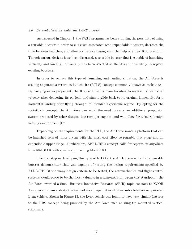
2.6 Current Research under the FAST program
As discussed in Chapter 1, the FAST program has been studying the possibilty of using
a reusable booster in order to cut costs associated with expendable boosters, decrease the
time between launches, and allow for flexible basing with the help of a new RBS platform.
Though various designs have been discussed, a reusable booster that is capable of launching
vertically and landing horizontally has been selected as the design most likely to replace
existing boosters.
In order to achieve this type of launching and landing situation, the Air Force is
seeking to pursue a return to launch site (RTLS) concept commonly known as rocketback.
By carrying extra propellant, the RBS will use its main boosters to reverse its horizontal
velocity after delivering its payload and simply glide back to its original launch site for a
horizontal landing after flying through its intended hypersonic regime. By opting for the
rocketback concept, the Air Force can avoid the need to carry an additional propulsion
system proposed by other designs, like turbojet engines, and will allow for a “more benign
heating environment.[1]”
Expanding on the requirements for the RBS, the Air Force wants a platform that can
be launched tens of times a year with the most cost effective reusable first stage and an
expendable upper stage. Furthermore, AFRL/RB’s concept calls for seperation anywhere
from 80-100 kft with speeds approaching Mach 5.0[1].
The first step in developing this type of RBS for the Air Force was to find a reusable
booster demonstrator that was capable of testing the design requirements specified by
AFRL/RB. Of the many design criteria to be tested, the aeromechanics and flight control
systems would prove to be the most valuable in a demonstrator. From this standpoint, the
Air Force awarded a Small Business Innovative Research (SBIR) topic contract to XCOR
Aerospace to demonstrate the technological capabilities of their suborbital rocket powered
Lynx vehicle. Shown in Figure 13, the Lynx vehicle was found to have very similar features
to the RBS concept being pursued by the Air Force such as wing tip mounted vertical
stabilizers.
17

Figure 13 XCOR Aerospace Lynx Vehicle Model[9]
The incorporation of similar flight conditions and vertical stabilizers mounted on the
wing tips make the Lynx vehicle a very good candidate for demonstration. In fact, of the
total twenty-nine technologies the Air Force was seeking to have demonstrated, the Lynx
vehicle alone was determined to provide nineteen of them. AFRL/RB and XCOR have
since established a cooperative research agreement (CRADA) that will allow both parties
to work together in order to develop their designs[1].
It is in this aspect that the work in this thesis takes shape. The ExFiT program has
been established to study and test the behavior of vertically-mounted wing tip stabilizers
incorporated in the design of the RBS in a hypersonic flight profile. Focusing on the
aeroelastic behavior of the wing tips, the geometry selected for this experiment very closely
resembled the geometry of the Lynx vehicle airfoil.
2.7 US Air Force Academy Partnership with AFIT
One of the final tasks left to setup this experiment was finding a platform with the
ability to allow testing of the wing and wing tip geometry selected in its proper flight regime.
With this in mind, the Air Force Institute of Technology (AFIT) has thus established a
working partnership with the US Air Force Academy and their FalconLAUNCH program.
18

This program was founded as a senior design project whereby senior cadets design, build,
and fly a sounding rocket over the course of one academic year.
Over the course of several years, AFIT has established a good working relationship
with the FalconLAUNCH program beginning with the aeroelastic fin optimization tool
developed by Joseph R. Simmons III for the cadets in order to prevent flutter with their
stabilizer fins. During the Spring of 2007, the Air Force Academy experienced a huge loss
when three of their four stabilizer fins sheared off of FalcoLAUNCH V due to flutter during
the launch. In his work, Simmons sought to avoid future flutter problems in the future by
developing a way to optimize fin design by varying the overall geometry, mass and material
of the stabilizer fins while still avoiding the onset of self-sustaining oscillations which lead to
flutter. By using various geometry optimization tools and flutter validation tools, Simmons
developed a cyclical design/iteration process to be followed for the design of stabilizer fins
used on successive FalconLAUNCH rockets [18].
Looking to widen the capabilities of FalconLAUNCH, the Academy has recently agreed
to attach experimental specimens to their rocket in order to collect data during the launch.
During the academic year 2008-2009, the design team of FalconLAUNCH VII attached a
small wing tip to the fuselage of the rocket. The shape of the fin tab is depicted in Figure
14. The overall size of the fin tab two and a quarter inches long.
In April of 2009, the FalconLAUNCH VII sounding rocket was successfully launched
and flew to an altitude of over 228000 feet at a max speed of Mach 4.8. Sadly, due to
computer malfunctions, data for this fin tip was unable to be collected or recorded. Although
no experimental data was returned, it was still impressive to note the performance of the
sounding rocket and the promise it would allow for future testing. Figure 15 shows the flight
profile of FalconLAUNCH VII.
For the academic year of 2009-2010, the new wing and wing tip geometry resembling
the XCOR Lynx vehicle has been selected to be attached to the next sounding rocket,
FalconLAUNCH VIII. However, because of the setbacks of last year, the design of this year’s
experiment was given top priority in terms of the Academy’s ability to return experimental
data. Due to the increase in size and complexity, the current experiment underwent a series
19
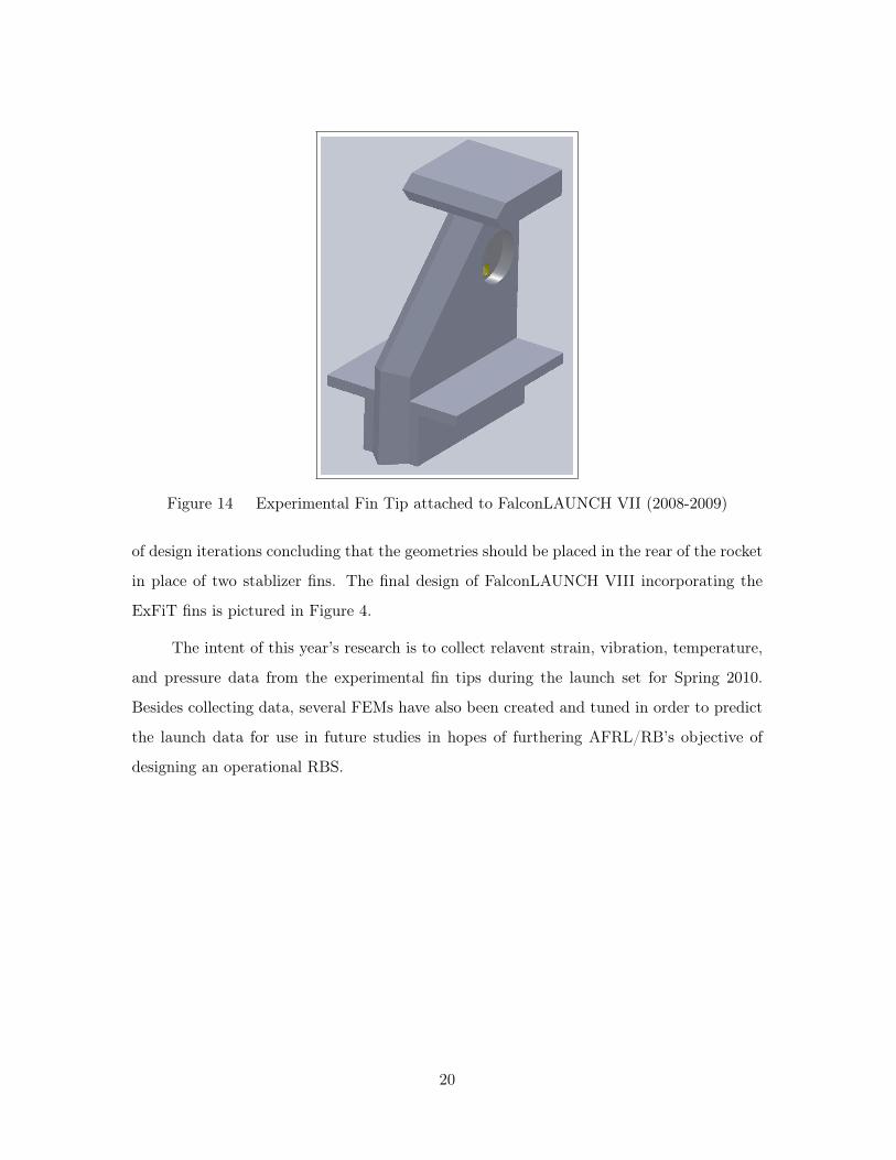
Figure 14 Experimental Fin Tip attached to FalconLAUNCH VII (2008-2009)
of design iterations concluding that the geometries should be placed in the rear of the rocket
in place of two stablizer fins. The final design of FalconLAUNCH VIII incorporating the
ExFiT fins is pictured in Figure 4.
The intent of this year’s research is to collect relavent strain, vibration, temperature,
and pressure data from the experimental fin tips during the launch set for Spring 2010.
Besides collecting data, several FEMs have also been created and tuned in order to predict
the launch data for use in future studies in hopes of furthering AFRL/RB’s objective of
designing an operational RBS.
20
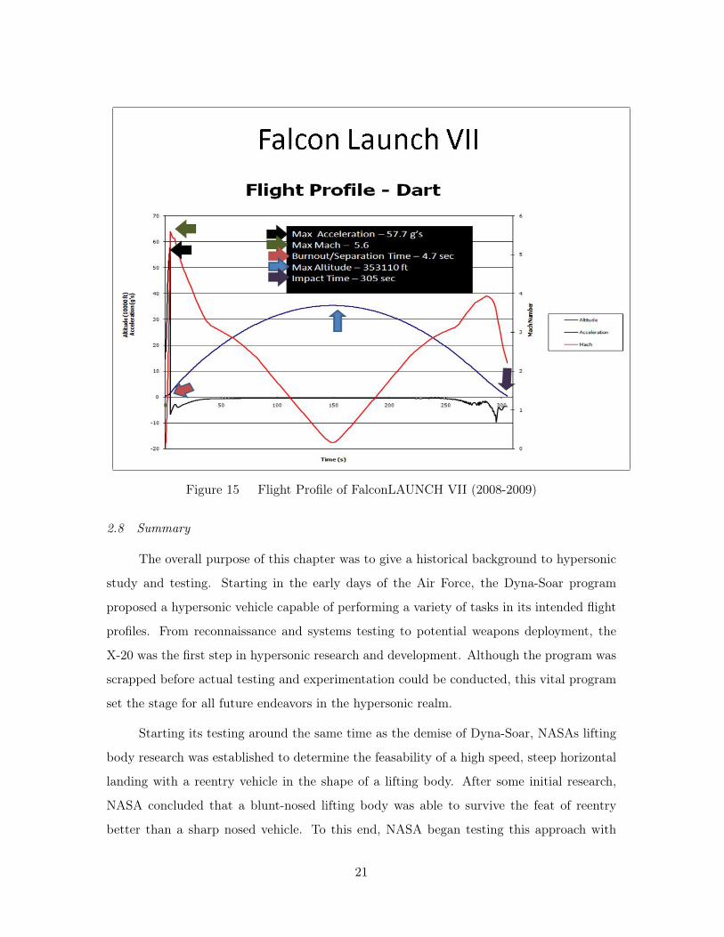
Figure 15 Flight Profile of FalconLAUNCH VII (2008-2009)
2.8 Summary
The overall purpose of this chapter was to give a historical background to hypersonic
study and testing. Starting in the early days of the Air Force, the Dyna-Soar program
proposed a hypersonic vehicle capable of performing a variety of tasks in its intended flight
profiles. From reconnaissance and systems testing to potential weapons deployment, the
X-20 was the first step in hypersonic research and development. Although the program was
scrapped before actual testing and experimentation could be conducted, this vital program
set the stage for all future endeavors in the hypersonic realm.
Starting its testing around the same time as the demise of Dyna-Soar, NASAs lifting
body research was established to determine the feasability of a high speed, steep horizontal
landing with a reentry vehicle in the shape of a lifting body. After some initial research,
NASA concluded that a blunt-nosed lifting body was able to survive the feat of reentry
better than a sharp nosed vehicle. To this end, NASA began testing this approach with
21

the M2-F1 and M2-F2 flight vehicles. After analyzing the results of these two vehicles,
NASA designed its final lifting body vehicle the HL-10 which underwent a series of subsonic
and low supersonic flight tests. After successfully completing all tasks required, the NASA
was able to confidently say that a lifting body was more than capable of surviving reentry
and performing the required horizontal landing. Although no actual hypersonic testing was
conducted, this program was able to provide crucial information and knowledge during the
development of NASA’s space shuttle orbital entry landing concept[13].
Next, the focus was shifted to more modern approaches of hypersonic study with
DARPA’s FALCON program and its hypersonic test bed the HTV-3X Blackswift. Revisiting
many of the goals and aspirations set forth with the X-20, DARPA’s Blackswift was another
proposed oppurtunity for designing an operational hypersonic weapons system. Fueled
by current military engagements, the HTV-3X was expected to carry out global bombing
missions within two hours of launch from inside the continental United States. However,
this program too was denied further funding before it could complete its testing.
Taking a look at current research studies, the internationally funded HIFiRE program
has been established to study the technologies necessary for hypersonic aerospace vehicles.
This program was started as a joint program between the Australian DSTO and AFRL
and continues to study and test various facets of hypersonic flight through sounding rocket
launches. The ultimate goal of this ongoing project is to continue to advance state-of-the-
art technologies and further the knowledge base of hypersonic flight. The lessons learned
from this cooperative research study can then be applied to future hypersonic vehicles or
reusable launch vehicles.
In the study at hand, the Air Force has deemed it necessary to fund the design of a
new booster system for its space launches. Through AFRL/RB and the FAST program,
the Air Force will begin to conduct hypersonic testing and experimentation in order to
design the new RBS. In conjunction with the Air Force Academy, this study will gather
experimental data on vertically mounted wing tips flown through a hypersonic regime by
means of a cadet-built sounding rocket, FalconLAUNCH VIII, in academic year 2009-2010.
The results of this study and future research in the ExFiT program intend to add to the
22

cumulative knowledge base regarding the design of the new RBS and hypersonic research
and development in general.
23

III. Methodology
3.1 Chapter Overview
This chapter will cover the progression of work on the experimental wing tips analyzed
for this experiment. First, a brief outline of the computational software used will be
discussed. From there, the pertinent design specifications for this experiment will be
discussed to include material properties and casting, sensor selection and location, and
placement on the rocket. From the final design specifications for FalconLAUNCH VIII, a
progression of computational finite element models will be discussed in terms of complexity
and mesh refinement. Validation of the finite element models was then conducted using
a ping test to validate computer calculated natural frequencies. Following this procedure,
an overview of the flutter analysis conducted by the Air Force Academy will be discussed.
This chapter will then conclude with an overview of the flight prediction tests conducted to
predict the strain, deflection, and heating effects experienced by the ExFiT fins during the
launch using the computational models.
3.2 Software used in this research
3.2.1 FEMAP v9.31. FEMAP, produced by Siemens PLM Software, is a pre
and post-processor of finite element models that comes paired with NX Nastran. FEMAP
can be used to create a variety of finite element models on which the desired analysis
can be performed. Results from FEMAP can include static, modal, thermal, buckling, and
stress/strain analyses. Apart from building models in FEMAP, this program can also import
various geometries created in other programs such as CAD and SolidWorks. This importing
feature gives the user the option to create the intended geometry in a way most familiar to
the operator. Once imported, the geometry can be given material properties, boundary
conditions, loading conditions and a finite element discretization before the analysis is
performed. When the finite element model is ready for analysis, the user can have FEMAP
run the analysis using the paired NX Nastran software. The program will then read the
results back into FEMAP whereby they can be displayed visually. FEMAP was used in this
research to find natural modes and frequencies, test various material properties and mesh
24
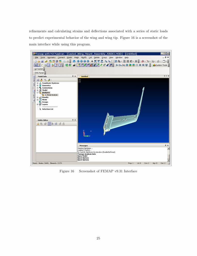
refinements and calculating strains and deflections associated with a series of static loads
to predict experimental behavior of the wing and wing tip. Figure 16 is a screenshot of the
main interface while using this program.
Figure 16 Screenshot of FEMAP v9.31 Interface
25

3.2.2 AeroFinSim v4.0. Classically, flutter is defined by the NASA Space Vehicle
Design Criteria as “a self-excited oscillation of a vehicle surface or component caused and
maintained by the aerodynamic, inertia, and elastic forces in the system [19].” Influenced
by a variety of variables including dynamic pressure, Mach number, mass distribution, total
mass, structural stiffness, and system dynamics, once flutter is initiated on a wing or fin it
usually leads to failure.
Although flutter can take on various forms, the most common form on a rocket is said
to be the two-dimensional, or bending-torsion, flutter manifested in the stabilizing fins in
the rear of the vessel. This occurs when the bending and torsional natural frequencies of the
wing or fin converge [20]. In order to avoid flutter, various equations have been developed to
predict the conditions that lead to its onset. Usually, the flutter velocity, Vf , and the flutter
dynamic pressure, Qf , are used to calculate the maximum velocity and pressure allowed
before a small disturbance in flight conditions would lead to the onset of flutter [21].
AeroFinSim v4.0, produced by AeroRocket, is a rocket fin aeroelastic analysis software
program that predicts both flutter and divergence velocity. This code uses a Theodorsen
method and U-g method dealing with structural damping and flight velocity to calculate
flutter velocity. Furthermore, this program also requires user inputs regarding the geometric
design, material property and mounting structure of the fin to accurately predict flutter
velocity, divergence velocity, and maximum allowable rocket velocity to ensure survivability
of the fins. The cadets at the Air Force Academy used this program in order to ensure
that the two stabilizing fins on the rocket as well as the experimental wing and wing tip
structures will not succumb to flutter or divergence. A more detailed look at the analysis
as well as the results from this program will be discussed later in this chapter. A screenshot
from the Users Manual of the results of a validation case for the program is presented below
[22]. From Figure 17, both the flutter velocity and divergence velocity were calculated and
graphed as a function of Mach number.
26

Figure 17 Screenshot of AeroFinSim v4.0 Results
3.3 Design Criteria for FalconLAUNCH VIII Experiment
Compared to the final design of the experiment attached to FalconLAUNCH VII
depicted in Figure 14, the current wing and wing tip geometry attached to FalconLAUNCH
VIII was much larger and more complex. In this section, a brief overview of the design
process will be discussed in order to highlight the key features of this year’s experiment to
include size and location of the experiment, materials proposed for the geometry, and sensor
types and locations.
3.3.1 Experiment Geometry Selection. Starting in the Summer of 2009, the initial
design specifications for this year’s experiment were discussed in great detail. The first
aspect acknowledged was that the design of the new experiment would have to be much
larger and more relevant to the design of the RBS that AFRL/RB was pursuing than
the fin tab attached to FalconLAUNCH VII (See Figure 14). From here, several new
geometries were analyzed, but ultimately, a geometry that closely resembles the XCOR Lynx
vehicle would be the goal seeing as XCOR and AFRL/RB had already developed a working
CRADA. After looking at the Lynx vehicle, it was decided that the geometry selected
27

would contain a delta wing configuration with a vertically mounted wing tip stabilizer.
This arrangement closely resembles the design of the FAST concept vehicle ensuring that
data collected on this experiment could be used to further research on the RBS.
3.3.2 Experimental Size and Location. Now that the geometry and overall shape
had been determined, location and size would prove to be critical in producing a successful
launch due to the aerodynamic impact this new geometry would impose on the sounding
rocket. Aerodynamically, the size and location determination process would have to go hand
in hand.
The first concept put forth by the Academy suggested including the experiment as an
attachment to the nose cone of the rocket. Essentially, the FalconLAUNCH team thought
that by keeping the size of the experiment to approximately 3 inches, the addition of two
experimental attachments to the nose cone could prove to be useful. The advantages and
disadvantages of this configuration were then considered in order to assess the viability of this
setup. As far as advantages were concerned, the two experiments would be exposed to clean
freestream air without being interrupted by the shock waves developing at the tip of the cone.
The data taken using this configuration would then closely resemble the arrangement of the
new RBS. However, the disadvantages of using this arrangement outweighed the usefullness
of this setup. With the addition of two experiments to the nose cone, the rocket’s stability
became a growing concern. In order to launch the rocket, the FalconLAUNCH team would
have to prove to the launch site that the rocket was stable and would not succumb to erratic
flight. Unable to do this in the allotted time, the FalconLAUNCH team scratched this idea.
The next concept proposed was to include two experimental attachments to the rear
of the rocket in place of two stabilizer fins. Once again, the advantages and disadvantages
were assessed. As far as the advantages were concerned, this configuration would allow a
simple attachment process similar to the mounting procedure already used on the stablizing
fins. Using a curved mount to match the curvature of the rocket, the experiment would
have to be cut or cast with this in mind so that it could simply slip into the mount and
be bolted in place. Second, the rear location of the experiment would allow for a test size
much greater than 3 inches. In this case, a simple a 1/10 scale of the original geometry
28

would allow for a test specimen size of approximately nine inches. This alone will enhance
the ability to collect relevant data. As an added benefit, the larger test specimen size will
also decrease the effect the actual rocket body will have on the behavior of each test section.
As far as disadvantages were concerned, the aerodynamic effects of the attachments
would have to be calculated using either wind tunnel or CFD simulations in order to account
for their effect on the rocket’s performance. Fortunately, the Academy has been able to
aquire both sets of simulations in order to address these questions. The Academy conducted
a set of wind tunnel tests on their own, and Second Lietenant Benjamin Switzer of AFIT
set up and ran CFD simulations as part of his thesis research [23]. From these two sources,
the Academy has been able to address the challenge of mounting the experiments at the
correct angle of attack as well as predicting their impact on the rocket’s flight to ensure
stability.
However, a second concern discussed was the fact that the experiments would not be
experiencing completely freestream conditions. However, it was established that the air will
travel through a shock cone and an expansion fan caused by the nosecone which will still
yield the hypersonic flight conditions intended for the experiment.
After discussing all of these points, the final location and size of the attachments were
decided upon. The experimental attachments would reflect the dimensions given in Figure
3 and located in place of two stabilizer fins as pictured in Figure 4.
3.3.3 Material Selection for the Experiment. After the size and shape of the
test specimen were decided upon, the material selection and production of the experiments
needed to be addressed. To begin, it was assumed that both the rocket and experiments were
to be made of the same material for ease of production and simplicity in design. Looking at
previous rockets, Aluminum 6061-T6 was selected due to its common usage in aircraft, its
high strength, and its availability. Similarly, this material was also common in most finite
element models in terms of material property cards.
However, the ability to cut the experiments in time for launch and cost of generating
the required number of attachments came into question. In order to get the parts in time for
testing and mounting, the design team at the Academy selected an independent company
29

to do the job. Located in Denver, Colorado, Prototype Casting, Inc. [24] was selected to
cast the fins in the proper time and within the allotted budget. In order to generate the
attachments, the company required a computer CAD model of the part. From here, they
used this model to perform various tasks to create a mold with which to use in the casting
process. To start, a Stereo Lithography Apparatus machine was used to build a plastic part
from the 3D file. In this process, a laser was used to solidify resin in layers to create the
part. Next, half of the stereo lithography apparatus model is put in clay while the other has
liquid rubber poured onto it. When the rubber is cured, they remove the mold and repeat
the process for the other half of the part. From here, they create a plaster mold using a
similar process. Lastly, molten aluminum is poured to create the finished part.
However, the disadvantage of using this company for the experiment was the fact that
they could not use Aluminum 6061-T6 as selected earlier in the design process. Instead,
they advertised the use of another material, Aluminum A357-T6, in its place. This material
was chosen because the company believed it was easier to perform the casting procedure
with this material as opposed to the original Al 6061-T6. In later sections, a comparison
between finite element natural frequencies with Al 6061-T6 and Al A356-T6 will show that
although there are slight differences in results, the material differences will not play a large
factor in the overall experiment. From here, Prototype Casting, Inc. then generated six
copies of the experiment with a set of two to be attached to the actual rocket, two for testing
at the Air Force Academy and two for use at AFIT. Shown in Figures 18 and 19 are pictures
of the actual casted wing and wing tip to be included in the launch of FalconLAUNCH VIII.
These pictures depict the model directly after production.
30

Figure 18 Casting Test Specimen Top View
31

Figure 19 Casting Test Specimen Angled View
32

3.3.4 Sensor Selection and Placement. Once the final designs for the size and
shape were selected, the type of sensors included on the experiment were then discussed.
After a few meetings, it was decided that strain and temperature gages would be included
on this year’s test in order to capture adequate temperature profiles and vibration data
that were desired from the launch. With these two parameters in mind, the inclusion of the
thermistors seemed intuitive. However, in order to capture the vibration data, strain gages
with a high sampling rate were chosen over competitive accelerometers for ease of mounting
due to size constraints and data collection.
In order to capture the behavior of both the wing and wing tip, both sensors were
included on the main wing portion and fin tip section as depicted earlier in Figure 5. In this
fashion, the data from the strain gages will then be used to capture the deflection of the test
specimen and the temperature gages will provide a heating profile. The flight prediction
tests conducted in Chapter 4 of this thesis will attempt to predict strain, deflection, and
heating effects incurred during the actual launch.
In order to accommodate the wiring necessary to include the gages, a sensor placement
patch and wire trough were cut into the experiment (see Figures 18 and 19 from previous
section). Once the gages and wires are in place, a ResinlabŹ EP 1200 black epoxy coating
will be applied to fill in and enclose the gages and wire trough to create a smooth surface
on the experiment. The epoxy has an approximate melting temperature of 400 degrees
Fahrenheit. However, due to an early setback in computational modeling, tests could not
be conducted to confirm the optimum placement of the gages. Therefore, it was decided that
they would be placed in the middle of both wing and wing tip sections of the test specimen.
However, it should be noted that in Chapter 5 of this report, a different location for the
strain and temperature gages will be recommended for future experiments. These decisions
were based on a modal analysis conducted to verify the mode shapes and deflections of the
fin.
Once the layout was decided, the Air Force Academy selected exact models for both
the strain and temperature gages. For the two strain gages, an Omega Karma brand SGK
SD3A-K350U shear gage was selected measuring approximately 8.5 x 9.8 mm. For the two
33

temperature gages, a Selco DT-A010K-1 thermistor was selected. Figure 20 depicts the two
specified gages as well as their individual make and model numbers.
(a) Omega Karma SGK SD3A-K350UStrain Gage
(b) Selco DT-A010K-1 Thermistor
Figure 20 Sensor Gages on Experiment
Overall, these gages were selected due to their ability to withstand the initial forces due
to rocket acceleration and their relative small sizes which made it easier for mounting to the
experiment. The Omega Karma SGK SD3A-K35OU strain gage has a nominal resistance
of 350 Ohms with a maximum permitted voltage of 15 Vrms. This specific gage has been
designed for usage on aluminum test specimens. The Selco thermistor has a resistance of
10000 Ohms at 25 Celsius, and a temperature range of -50 to 250 Celsius.
3.4 Flutter Analysis
Although flutter can take on various forms, the most common form on a rocket is said
to be the two-dimensional, or bending-torsion, flutter manifested in the stabilizing fins in
the rear of the vessel. This occurs when the bending and torsional natural frequencies of the
wing or fin converge[20]. In order to avoid this phenomenon, various equations have been
developed to predict the conditions that lead to its onset. After prediction, the flight profile
of the rocket can then be varied to avoid a flight scenario that could lead to its failure.
For the test specimen attached to FalconLAUNCH VIII, the cadets in the design
team used AeroRocket’s AeroFinSim v4.0 to conduct a flutter analysis. The cadets used
this program with a built in Theodorsen calculation to predict the flutter velocity of the
part. However, because AeroFinSim was developed as a rocket fin flutter tool, the cadets
34

were not able to conduct a flutter analysis on the entire test specimen as a single piece.
Instead, the cadets opted to divide the geometry into two seperate pieces: the main wing
section and the fin tip section. After giving the program the specifications and dimensions
of each piece of the payload, they used the program to calculate the flutter velocities of each
seperate piece. The results from these tests are presented in Chapter 4.
3.5 FEM Progression and Initial Analysis
Now that all the design specifications of the test specimen had been determined,
accurate finite element models were produced using FEMAP v9.31. In this section of the
chapter, the progression of finite element models will be discussed in detail in order to
highlight the attributes of each successive model. As an overview, the models created
increase in complexity and accuracy. The first few models are the earliest attempts and are
therefore the least accurate. The later models will demonstrate a higher level of knowledge
of FEMAP and will include a more detailed meshing.
3.5.1 Flat Plate Models. As a first attempt at creating the finite element models,
flat plate models were created using plate elements with a specified thickness representing
the average thickness of the test specimen. The flat plate models reflect the overall shape
of the test specimen, but lack the detailed wing shape and curvature of the actual geometry
and are inherently inaccurate. However, these first iteration models were only truly intended
to provide back of the envelope approximations of modal frequencies and shapes in order
to help the Academy’s avionics team determine the sampling rate of the strain gages early
in the design process.
The first model created was a 1/10 scale model measuring approximately nine inches
in length and was made up of three flat plates representing each section of the test specimen:
the main wing portion, the connecting elbow, and the vertical wing tip. From here, the flat
plates were given the material properties of Aluminum 6061-T6 as depicted by the original
design specifications of the test specimen. Next, the plates were divided into 10 simple
elements from 18 nodes defined in the geometry. Figure 21 depicts a screenshot of the first
flat plate model.
35

Figure 21 First Flat Plate Model
The second model created was basically an extension of the first model in terms of
overall geometry. The only difference between the second model and the first is the more
accurate mesh on the flat plates. In order to generate this mesh, the program’s automesh
feature was used to add more accuracy and definition to the model. After the automesh
feature was utilized, more elements were added to the section thought to have the most strain
associated with it: the union of between the main wing and the vertical wing tip stabilizer.
Depicted in Figure 22, the second flat plate model contains 269 generated elements and 270
nodes. Once again, the purpose of the flat plate models was to provide back of the envelope
approximations of the natural frequencies and mode shapes to provide adequate sampling
rates for the avionics team.
3.5.2 Meshing Complex Geometries. After the flat plate models had been ana-
lyzed, more accurate models needed to be created for more accurate analysis. However,
one of the reasons a full wing geometry was not originally modeled was due to a failure
in the automesh feature in FEMAP which needed to be riddled out. Essentially, when the
36

Figure 22 Second Flat Plate Model
automesh feature was utilized, an error would occur stating that the mesher was aborted
and that the surface contained at least one hole. Figure 23 depicts the mesh abort message
as well as one of the holes visable in the surface. In order to generate an appropriate solid
mesh, the surface would have to be patched before the program could generate a solid mesh
from the watertight surface.
For a few weeks, a solution to this problem could not be found. However, after detailed
troubleshooting a solution was discovered whereby new nodes had be created from existing
ones nearby in order to fill in the empty spaces in the surface. These errors were believed
to originate from the lack of detail in the geometry that defined the surface of the test
specimen. Rather than specifying the exact coordinates for the new nodes that made up
the surface, the vector between a set of similar nearby nodes was copied and used to offset
the new node from the copied one. Figure 24 shows the new node created from the pair
indicated by the red circle.
37

Figure 23 Surface Hole
Figure 24 New Surface Node
Once the new node was created, the existing elements surrounding the hole were
deleted and new ones were manually created and connected to create the ”watertight” mesh
required. Figure 25 depicts the fixed mesh that was then used for further analysis. Finally,
the entire process was repeated three more times to fix all the holes in the surface. Once
this was done, the program was able to generate a solid mesh of the entire part from the
newly closed surface.
38

Figure 25 New Fixed Surface - No Hole
3.5.3 Full Wing Models. Now that the problem with the full wing surface was
solved, new models were created to increase the accuracy and relevancy of the results
obtained from them. Using the automesh feature on the closed surfaces, the solid mesh
was generated on the model. Once again, these models were originally made of the Al
6061-T6 material specified early on in the design process. Later sections will discuss the
changing of the material properties from Al 6061-T6 to Al A357-T6 and the implications
associated with the change.
The first full wing geometry modeled is shown in Figure 26. This model contained
1326 elements and 2837 nodes that made up the actual geometry.
Although the first full wing model was able to improve the accuracy of the results from
the original flat plate models, it was still lacking the additional effects from the mounting
structure and the grooves cut into the test speciment. The next model was created to
simulate these two characteristics of the exact test specimen. In that light, the results
obtained from this model will accurately reflect the true launch conditions and experimental
setup. This model will later be used to conduct the flight prediction tests using loads
predicted from CFD outputs and a static loading analysis run with NX Nastran. The
model also contains a more detailed mesh containing 21372 elements from 36481 nodes that
comprise the geometry of the wing and mounting bracket. Figures 27 and 28 show two
views of the new model with the mounting bracket attached.
39

Figure 26 First Full Wing Model
Figure 27 Final Full Wing Model
40

Figure 28 Additional View of Model
41
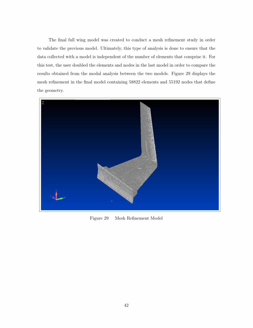
The final full wing model was created to conduct a mesh refinement study in order
to validate the previous model. Ultimately, this type of analysis is done to ensure that the
data collected with a model is independent of the number of elements that comprise it. For
this test, the user doubled the elements and nodes in the last model in order to compare the
results obtained from the modal analysis between the two models. Figure 29 displays the
mesh refinement in the final model containing 58822 elements and 55192 nodes that define
the geometry.
Figure 29 Mesh Refinement Model
42

3.5.4 Modal Analysis of FE Models. In this section, the first three natural
frequencies and mode shapes of each finite element model were calculated using the NX
NASTRAN Normal Modes/Eigenvalues analysis feature included in FEMAP v9.31. In the
program, the user set the boundary conditions such that the ends of each model were fixed
and could not move in any direction. The intent here was to simulate the experiment being
attached to the rocket or fixed bench mount much like a cantilevered beam. The results of
this analysis are presented in Table 1. In this table, the results are broken down between
each flat plate model and the two full wing models.
Table 1 First three natural frequencies(Hz) of FE models using Al6061-T6Mode Flat Plate 1 Flat Plate 2 Full Wing 1 Final Model1 75.1 78.4 103.4 103.72 175.5 185.6 201.6 194.33 233.9 245.9 338.8 360.6
It is evident from this analysis that the flat plate models were not as accurate as
originally thought. When compared to the full wing models, it is clear that there are large
differences in calculated natural frequencies. In their defense, however, their intent was not
accuracy but rather a way to provide the avionics team an order of magnitude estimate for
the sampling rate of the strain gages. In that regard, they were able to serve their purpose.
The sampling rate for the strain gages was set to 500Hz. For actual flight prediction,
however, a full wing model must be used.
The next piece of information to take away from this modal analysis was the com-
parison between the two full wing models. Looking at the first mode, there was only a
0.3% difference. However, the next two modes result in a 3.7% and 6.2% difference in their
frequencies, respectively. Although the differences are not extreme, it is clear that adding
the mounting bracket and cuts into the geometry for the gages and wires does indeed make
a difference in the results. For this reason, the flight prediction tests will be done with the
final full wing model presented in Figure 27.
3.5.5 Material Property Comparison. This section will address the effect of
changing the material property of the full wing models after it was determined that the
43

test specimens were to be cast out of Aluminum A357-T6 instead of Aluminum 6061-T6 as
originally thought.
Once the different FE models were created, changing the material property cards in
FEMAP was relatively simple. With the model open in FEMAP, a new material property
card was created and titled Al A357-T6. Next, the material properties were referenced via
the published data on Matweb [25]. In the new material card, the Young’s Modulus, Shear
Modulus, Poisson’s Ratio, Limit Stress Tension, Compression, Shear, and Mass Density
were adjusted. Figure 30 depicts the new material card used by FEMAP to simulate Al
A357-T6. Once this new card was created, it was activated so that the model was entirely
composed of the new cast material. This process was repeated twice in order to update
both full wing models.
Figure 30 Al A357-T6 Property Card Creation
The results from the new modal analysis tests are presented in Table 2. In the table,
the results are broken down by model with the natural frequencies corresponding to each
mode presented side by side for easier comparison. From the results, the percent difference
44

between the calculated natural frequency in the new material and the original material never
rises higher than 3.7%. This indicates that using the new Al A357-T6 material will not have
a drastic effect on the results obtained with it. From this point on, the flight prediction
tests for FalconLAUNCH VIII will be conducted using the model composed of Al A357-T6.
Table 2 Natural Frequencies (Hz) of Different MaterialsFull Wing 1 Final Model
Mode Al6061-T6 Al357-T6 % Diff Mode Al6061-T6 Al357-T6 % Diff1 103.4 107.3 3.7 1 103.7 107.6 3.72 201.6 209.2 3.6 2 194.3 201.6 3.73 338.8 351.7 3.7 3 360.6 374.3 3.7
3.5.6 Mesh Refinement. The final aspect covered regarding FE model generation
was a simple mesh refinement study. This test was conducted to ensure that the results
obtained using the final full wing model were not subject to a lack of accuracy due to the
number of elements in the model. For this test, the models depicted in Figures 27 and 29
were used and the natural frequencies for each mode were compared. Table 3 displays the
results of the mesh refinement study. It is important to note that the new Al A357-T6
material card was used for this study and for all future tests.
Table 3 Mesh Refinement StudyMode Final Model(Hz) Mesh Refined Model(Hz)1 107.6 107.62 201.6 201.63 374.3 374.3
From these results, there were no differences in the natural frequencies calculated in
FEMAP between the final model and the mesh refined model. This indicates that doubling
the number of elements had no effect on the results of this test. However, the only difference
between the two models came in computational time required to calculate the results. The
mesh refined model took twice the time to process than the final model. Therefore, because
there was no change in results and because the final model takes less computational time
to process, the final full wing model will be used for all flight prediction testing.
45
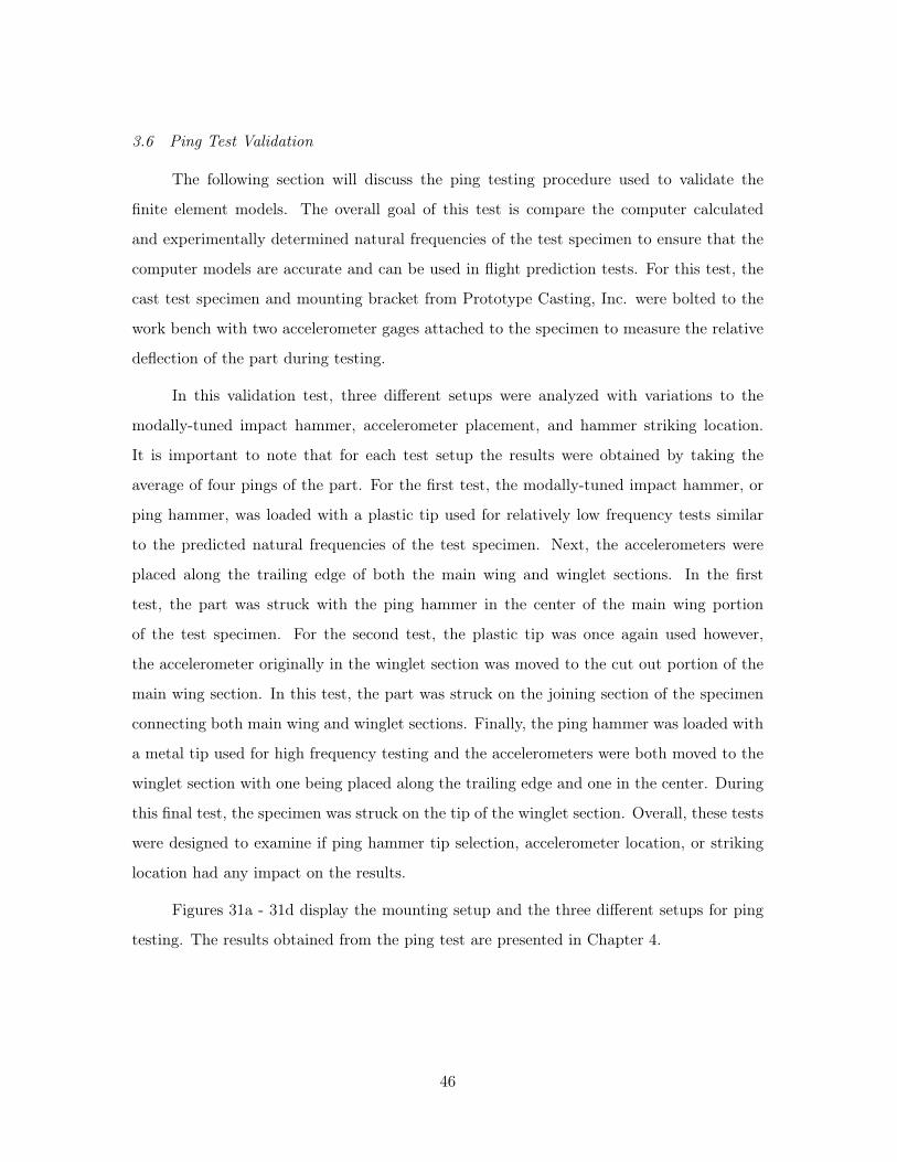
3.6 Ping Test Validation
The following section will discuss the ping testing procedure used to validate the
finite element models. The overall goal of this test is compare the computer calculated
and experimentally determined natural frequencies of the test specimen to ensure that the
computer models are accurate and can be used in flight prediction tests. For this test, the
cast test specimen and mounting bracket from Prototype Casting, Inc. were bolted to the
work bench with two accelerometer gages attached to the specimen to measure the relative
deflection of the part during testing.
In this validation test, three different setups were analyzed with variations to the
modally-tuned impact hammer, accelerometer placement, and hammer striking location.
It is important to note that for each test setup the results were obtained by taking the
average of four pings of the part. For the first test, the modally-tuned impact hammer, or
ping hammer, was loaded with a plastic tip used for relatively low frequency tests similar
to the predicted natural frequencies of the test specimen. Next, the accelerometers were
placed along the trailing edge of both the main wing and winglet sections. In the first
test, the part was struck with the ping hammer in the center of the main wing portion
of the test specimen. For the second test, the plastic tip was once again used however,
the accelerometer originally in the winglet section was moved to the cut out portion of the
main wing section. In this test, the part was struck on the joining section of the specimen
connecting both main wing and winglet sections. Finally, the ping hammer was loaded with
a metal tip used for high frequency testing and the accelerometers were both moved to the
winglet section with one being placed along the trailing edge and one in the center. During
this final test, the specimen was struck on the tip of the winglet section. Overall, these tests
were designed to examine if ping hammer tip selection, accelerometer location, or striking
location had any impact on the results.
Figures 31a - 31d display the mounting setup and the three different setups for ping
testing. The results obtained from the ping test are presented in Chapter 4.
46

(a) Mounting Setup and Ping Hammer (b) 1st Test Setup
(c) 2nd Test Setup (d) 3rd Test Setup
Figure 31 Ping Test Experimental Setup
47

3.7 Flight Prediction using FEMs
Now that the FE models have been tested and validated, they were then modified to
predict the strain data collected by the strain gages as well as provide deflection data and
heating effects of the flight on the actual test specimen. As an overview, the final FEM
presented in Figure 27 has been sliced into several different surfaces to have the predicted
pressure loads applied to it. In order to estimate these pressure loads, several computational
fluid dynamic(CFD) simulations have been analyzed to attain the correct distribution of
pressure over the wing and wing tip sections of the experiment. This section will conclude
with a brief description of how the loads were placed on the model, how the static analysis
was conducted to obtain strain and deflection data in FEMAP, and how heating will affect
the results obtained.
3.7.1 FEM Modifications. To place the pressure loads on the FE model, the top
surface of the final full wing model had to be cut into several different surfaces. Basically,
there are two ways to apply loads to a model in FEMAP: node by node or onto an entire
surface. In order to eliminate a painstaking process of clicking thousands of different nodes
and applying the forces, these surfaces can be used to represent each node within the
surface. From here the predicted CFD pressure loads will then be placed on these newly
sliced surfaces of the model. By creating eight surfaces on the main wing section and two on
the vertical stabilizer, ten different pressure distributions can now be placed on the model.
To illustrate this process, a series of figures were created to highlight the steps taken
to slice the model into the desired surface configuration. Figure 32a shows the untouched
model before the slicing process began. Figure 32b in the series shows how the first cut
was made by using the points already in the model used to cut out a location for the strain
gage and wire trough. In this manner, it was necessary to include three points to properly
dictate how to cut the solid. The first two points selected were oriented on the top surface
of the wing which dictated the location of the cutting plane. The third point was located
at the base of the recessed region of the model which indicated how to orient the cutting
plane. Using this arrangement, FEMAP sliced the model from leading to trailing edge and
48

resulted in two new surfaces. Figure 32c in the series displays the two new surfaces. In the
figure, one surface has been selected and the second is highlighted by the cursor.
From here, three new points were placed on the desired curves of the model. Figure
32d indicates that one point was placed on the back of the wire trough channel and two
others were placed along the midpoint of the curves defining the trailing edge of the wing.
Also displayed in this figure is the resulting cutting plane that has been defined by the three
new points. Figure 32e shows the two new created surfaces from the slice; both have been
highlighted for better viewing.
In this fashion, the finite element model has been sliced several more times resulting in
8 surfaces that define the main wing portion of the specimen and two surfaces that define the
wing tip portion. The final figure in the series, Figure 32f shows the resulting configuration
of the model after all necessary cuts were made.
3.7.2 Flight Profile Test Points. Once the FE model was ready to have pressure
loads applied to the surfaces, it was necessary to decide which points during the flight profile
to analyze. To begin this process, the flight profile for the current launch was provided by
the Air Force Academy and studied. Figure 33 depicts the proposed profile.
After viewing this profile, it was decided that a total of five points from the profile
would be included for further studying. These five points were selected to cover a wide
range of flight conditions that sample the acceleration and deceleration of the rocket as it
continues to gain altitude. The first three points cover the acceleration of the rocket starting
at Mach 1.0 and leading up to Mach 4.5. The last two points occur during deceleration and
conclude with a final speed of Mach 1.0. The five test points have been highlighted on the
flight profile as depicted in Figure 33 with an arrow pointing to each respective test case.
Although some of the test points occur at similar Mach numbers, the difference in
altitude and ambient pressure with each test point resulted in differing Reynolds numbers
for each respective test. The points selected for study have been chosen for their various
implications on the test specimen during the flight. The first two points should capture the
erratic nature of the rocket during its acceleration. The next three points should capture the
loading of the payload close to its highest anticipated speed and the loading at the highest
49

(a) Pre-Slicing Geometry (b) Step 1
(c) Step 2 (d) Step 3
(e) Step 4 (f) Post-Slicing Geometry
Figure 32 FEM Slicing Progression from Top Left to Bottom Right
altitudes. Table 4 presents the data points to be studied from the published FalconLAUNCH
VIII profile. In this table, the Mach number, altitude,ambient pressure, and the Reynolds
number associated with each test point is included.
3.7.3 CFD Analysis. In order to calculate the pressure distribution over the main
wing and wing tip sections of the test specimen at the five test points, Second Lieutenant
Benjamin Switzer conducted a CFD analysis using an AFRL code called AVUS [23]. In his
work, Lieutenant Switzer catagorized the performance of the test specimen throughout its
intended flight profile for a variety of angles of attack. After conducting his simulations,
50

Figure 33 Flight Profile for FalconLAUNCH VIII
Table 4 Flight Profile Data Points for FE TestingTest Number Mach Number Altitude (kft) Pressure (kPa) Reynold’s #
1 1.0 5 84.312 3.369E62 2.5 9 72.428 7.509E63 4.5 30 30.148 6.996E64 2.5 60 7.231 1.003E65 1.0 100 1.105 5.580E4
the results of his runs were then used to generate lift and drag versus angle of attack curves
(Cl vs. α and Cd vs. α).
Aside from these generated lift and drag curves, the output files from the AVUS code
were then used to calculate the flight pressure loads on the test specimen for the selected
points presented in Table 4. From here, the calculated loading pressures were then used on
51

each FE model in the flight prediction analysis. The actual results obtained from the CFD
analysis are located in Chapter 4 of the report.
3.7.4 Heating Effect. In this subsection, the effect of heating will be discussed.
During the launch, the test specimen will incur a great deal of heating due to the hypersonic
speeds the rocket will reach. That being said, the material properties of the test specimen
will vary accordingly. In order to predict some of the changes that may occur to the test
specimen, a series of modal analyses will be conducted in order to see the general effect
of heat on the calculated natural frequencies of the part. Ultimately, the purpose of these
tests will be to see how decreasing the Young’s Modulus affects the first and second natural
frequencies. In terms of flutter, the first and second natural frequencies should remain as
far from each other as possible[18]. However, it is expected that by lowering the Young’s
Modulus, the two values will actually grow closer together. In future experiments, different
materials should be tested in order to avoid this phenomenon.
In general the Young’s Modulus, or Modulus of Elasticity, of aluminum will decrease
as the testing temperature of aluminum increases [26]. In order to conduct this test, the
modulus of elasticity was varied from its intial reference value of 10.5 E6 psi to a value that
is 20% lower corresponding to a temperature increase to 600 degrees Celsius. This was done
to approximate the effect the increasing temperature will have on the part. Ultimately, the
heating profile of the part is still unknown, so by approximating the effect of heating up
to 600 degrees Celsius the test will capture the results on the specimen up to the melting
point of the material. Overall, this test will demonstrate the general effect that the lower
values will have on the calculated natural frequencies up until the failure of the material.
Specifically for this test, the material card for Al A357-T6 was modified so that the
Young’s Modulus was lowered by intervals of 5% down to its final value of 20%. The model
was then regenerated to reflect the changes in the properties of the elements that comprise
it. From here, NX Nastran was used to calculate the natural frequencies in a modal analysis
in FEMAP. Table 5 displays the different values of Young’s Modulus tested. The results
from these tests will be presented in Chapter 4.
52

Table 5 Young’s Modulus Variation for Heating EffectTest Number Reduction Value (%) Young’s Modulus (psi)
1 0.0 10.5 E62 5.0 9.975 E63 10.0 9.45 E64 15.0 8.925 E65 20.0 8.4 E6
3.8 Chapter Summary
In this chapter, the methodology done to setup the various flight prediction tests using
the finite element models was discussed. Beginning with a brief description of the software
programs used in this thesis and overall an description of flutter on rocket fins, this chapter
then discussed the design process undertaken to setup the actual payload that is going to
be attached to body of the sounding rocket. Following this, the progression of finite element
models built in FEMAP and the problems encountered in their construction were outlined.
Next, obstacles in the automesh feature in FEMAP were described as well as their solutions.
By fixing the surface mesh in the full wing models, more accurate and detailed finite element
models and meshes were then created for further testing to include a mesh refinement study,
heating analysis and flight prediction tests. In order to validate the finite element models, a
ping test was conducted in order to compare the experimentally determined and computer
calculated natural frequencies to ensure the computer models were accurate and valid for
use in the flight prediction tests. In these prediction tests, results for strain gage prediction,
test specimen deflection, and heating effects were analyzed with the results presented in the
next chapter. Overall, the finite element models are looking to predict the data collected by
the test specimens attached to the rocket in order to validate the results collected through
these tests.
53

IV. Results for FalconLAUNCH VIII Flight Prediction Experiments and Future
Models
4.1 Chapter Overview
This chapter will be broken into several different sections regarding the results from
this year’s tests. The first section will discuss the results obtained from the AeroFinSim
flutter analysis program used by the cadets at the Air Force Academy. Next, the results from
the ping validation test will be presented along with a comparison between the computer
and experimental models. The next section will address the challenges associated with the
set-up of the flight prediction tests in FEMAP stemming from the surface loads applied to
the model. The following section will then describe the solution to this problem and the
final procedure used to conduct the tests. The fifth section will present the results from the
FE analysis to include strain gage predictions, test specimen deflections, and heating test
results. The final section will describe a potential carbon-fiber model created to anticipate
next year’s experiment along with some initial results obtained with the new model to
include strain gage prediction and test specimen deflections.
4.2 AeroFinSim Results
Using the AeroFinSim rocket fin flutter analysis program, the cadets at the Academy
obtained promising results. Overall, the program projected that neither piece of the payload
would reach its respective flutter velocity. Due to the limitations of AeroFinSim, the cadets
could not model the test specimen as a single piece and have therefore conducted two
seperate analyses on each respective part. The dimensions input into the program are
shown in Table 6.
Table 6 Dimensions of Test Specimen Sections Used in AeroFinSim (in.)Main Wing Section Winglet Section
Root Chord 9.2 4.0Tip Chord 3.5 2.5Semi Span 7.0 6.0Sweep 6.5 3.5
Body Diameter 7.1 7.1Thickness 0.75 0.25
54

Using these dimensions for each part of the test specimen, the program produced the
following flutter results presented in Table 7. The table shows the flutter velocity as a
function of Mach number for each altitude in the flight profile of the rocket. From these
results, neither section of the test specimen would undergo flutter.
Table 7 AeroFinSim Flutter ResultsAltitude Main Wing Section Winglet Section[kft] [Mach Number] [Mach Number]0 12.28 4.695 13.4 5.1410 14.26 5.4815 16.11 2.520 17.76 6.8825 19.66 7.6430 21.85 8.5335 24.42 9.5740 27.39 10.7845 30.64 12.1450 34.57 13.66
Figure 34 has been produced by the cadets to visually display the results obtained
from AeroFinSim. The flutter velocity of both the main wing section and the wintip section
has been plotted. In the same manner, the relevant portion of the flight profile has also
been graphed to show that the flutter velocities of each respective section are not within the
intended launch profile. Overall, the results calculated using AeroFinSim suggest that the
test specimen attached to FalconLAUNCH VIII will not fail due to fluttering. However, the
assumptions made to conduct this analysis are somewhat questionable. The full implications
of these results are discussed in Chapter 5.
55

Figure 34 AeroFinSim Flutter Results
4.3 Ping Test Results and Comparisons
The results from the ping tests on the experimental part are presented with respect to
each different testing setup. Important to note is the fact that the results are presented as
an average of four different tests, or pings, for each different experimental setup. The first
set of results deals with the first test setup with a plastic tipped ping hammer striking the
center of the main wing section and accelerometers located on the trailing edges of both main
wing and winglet sections. The second set of results was obtained using the same plastic
tipped ping hammer striking the elbow of the test specimen with accelerometers located on
the trailing edge and center of the main wing section. The final test was conducted using
a metal tip mounted on the ping hammer which struck the part on the tip of the winglet.
The accelerometers for this test were located on the trailing edge and center of the winglet
section of the payload. The results from these three tests are presented in Figures 35-37
which display the natural frequencies of the payload as well as each corresponding phase
56

and cohesion plot. Along with these plots, the input and time history of each test are also
presented.
(a) Natural Frequency, Phase and Coherence
(b) Hammer Input (c) Time History
Figure 35 Results from 1st Ping test
57
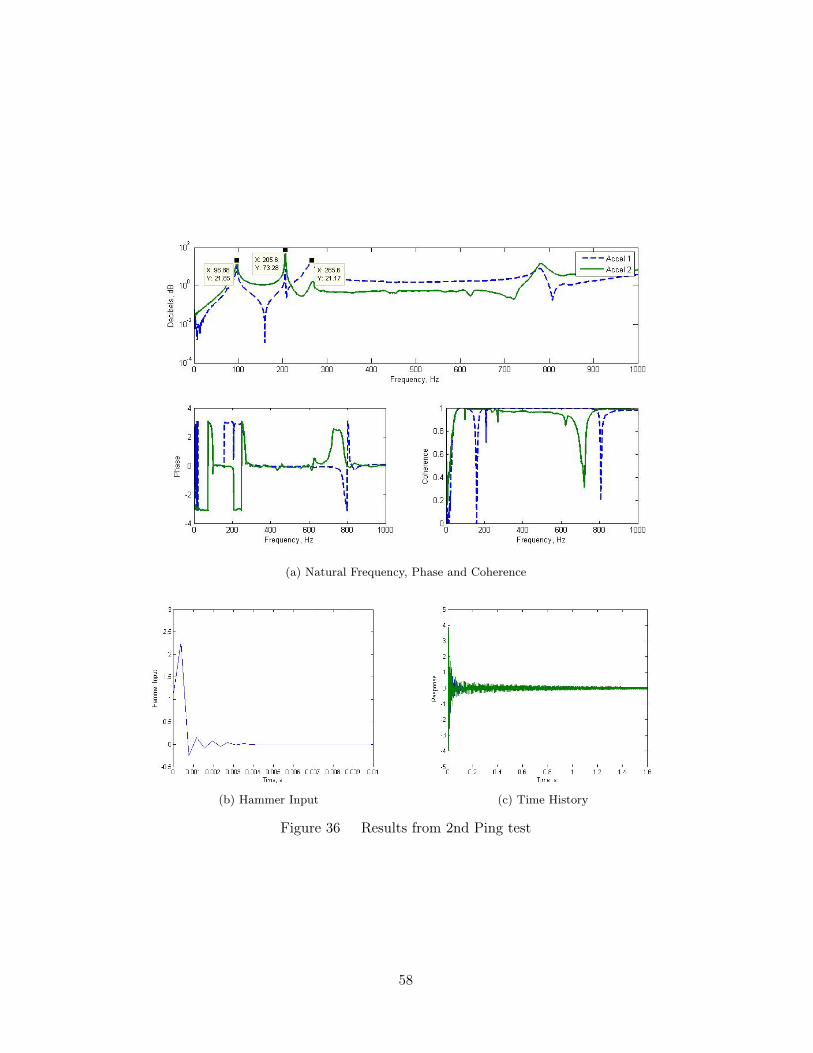
(a) Natural Frequency, Phase and Coherence
(b) Hammer Input (c) Time History
Figure 36 Results from 2nd Ping test
58

(a) Natural Frequency, Phase and Coherence
(b) Hammer Input (c) Time History
Figure 37 Results from 3rd Ping test
59
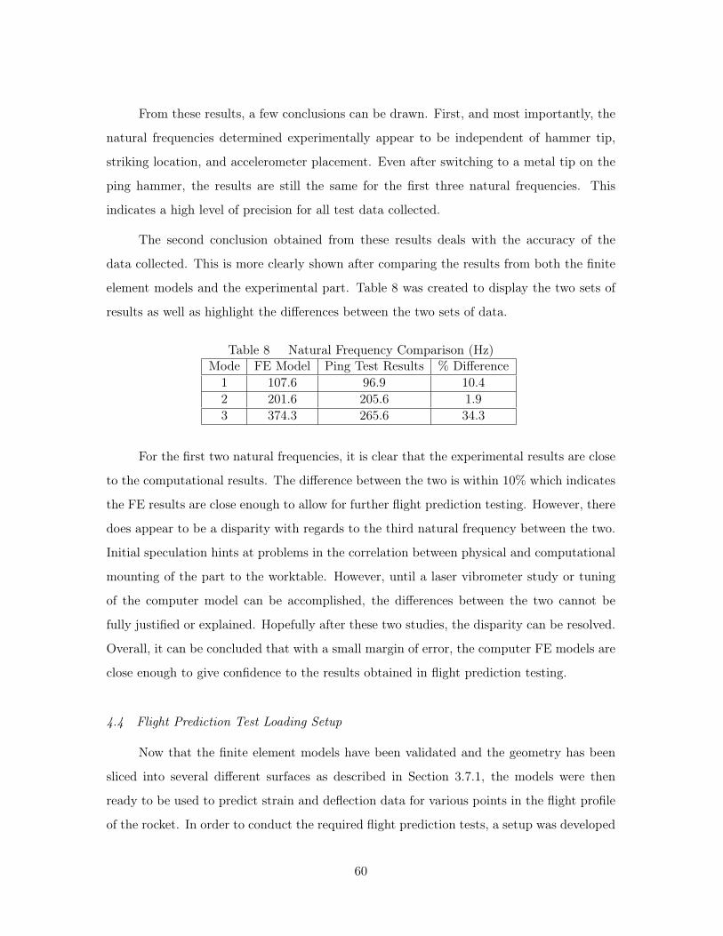
From these results, a few conclusions can be drawn. First, and most importantly, the
natural frequencies determined experimentally appear to be independent of hammer tip,
striking location, and accelerometer placement. Even after switching to a metal tip on the
ping hammer, the results are still the same for the first three natural frequencies. This
indicates a high level of precision for all test data collected.
The second conclusion obtained from these results deals with the accuracy of the
data collected. This is more clearly shown after comparing the results from both the finite
element models and the experimental part. Table 8 was created to display the two sets of
results as well as highlight the differences between the two sets of data.
Table 8 Natural Frequency Comparison (Hz)Mode FE Model Ping Test Results % Difference1 107.6 96.9 10.42 201.6 205.6 1.93 374.3 265.6 34.3
For the first two natural frequencies, it is clear that the experimental results are close
to the computational results. The difference between the two is within 10% which indicates
the FE results are close enough to allow for further flight prediction testing. However, there
does appear to be a disparity with regards to the third natural frequency between the two.
Initial speculation hints at problems in the correlation between physical and computational
mounting of the part to the worktable. However, until a laser vibrometer study or tuning
of the computer model can be accomplished, the differences between the two cannot be
fully justified or explained. Hopefully after these two studies, the disparity can be resolved.
Overall, it can be concluded that with a small margin of error, the computer FE models are
close enough to give confidence to the results obtained in flight prediction testing.
4.4 Flight Prediction Test Loading Setup
Now that the finite element models have been validated and the geometry has been
sliced into several different surfaces as described in Section 3.7.1, the models were then
ready to be used to predict strain and deflection data for various points in the flight profile
of the rocket. In order to conduct the required flight prediction tests, a setup was developed
60

to convert the distributed loads on the sliced surfaces to resultant forces located in the
centroid of each newly sliced surface. Using the “Section Properties” command under the
“Tools” menu, the location of the centroid and area of each surface were calculated. Using
the coordinates of the centroid, a point was then created at that location using a series of
workplane orientations for each new surface. Figure 38 shows a few of the created points in
the centroid of three of the sliced surfaces.
Figure 38 Point Created in Surface Centroid
After the centroidal points were created in all 10 surfaces, a force was then placed on
the node lying closest to each centroid. From here, the calculated area of each surface was
multiplied by the pressure force specified by the CFD analysis at that point to calculate
the resultant force for each surface. In other words, this method simply converted the
distributed pressure loads on each surface into resultant point forces that FEMAP was able
to use in the NX Nastran static analysis feature.
In summary, by applying resultant forces to the centroid of each surface, the static
analysis was able to calculate the resulting strain and deflection at each node on the payload.
61

4.5 Flight Prediction Results
In this section, the results from the flight prediction tests will be presented to highlight
strain gage predictions and part deflections for each test point in the flight profile. However,
to start these tests, the results of the CFD analysis were used to calculate the resultant forces
that were applied to the centroid of each surface on the model. This section will discuss
each necessary step in obtaining these flight prediction results.
4.5.1 CFD Results. Using AFRL’s AVUS code, 2Lt Switzer ran many CFD
simulations that encompassed the flight profile of the test specimen as depicted in Figure
33 [23]. By analyzing his results, Switzer was able to recommend mounting the payload at
an angle of attack of three degrees in order to meet the requirements put forth by the Air
Force Academy for their flight profile calculations. Namely, the cadets had to ensure the
sounding rocket would spin at a rate 4 Hz by using the predicted lift and drag coefficients
produced by Switzer. By establishing this setup, Switzer was able to properly model the
flight profile of this year’s launch.
Next, the CFD output for each flight test point was analyzed. Using the output file
from the code, the pressure at each centroidal point in the 10 surfaces was found in units of
dynes/cm2 for each of the five test cases corresponding to Table 4. From here, the pressure
was converted to psi and then multiplied by the area associated with each surface to calculate
the resultant forces. Tables 9-13 show the pressures and areas associated with each surface
of the model for the five test cases analyzed. These five test cases have been selected to
cover the acceleration and deceleration of the rocket and are further outlined in Section
3.7.2 and in Table 4. Looking at the resultant forces, it is clear that the acceleration of the
rocket up to its top speed will generate the largest forces on the test payload. Similarly,
these acceleration test points are expected to generate the largest deflections and strain
readings calculated in FEMAP.
62

Table 9 5k, Mach 1.0 Test ConfigurationSurface Number Area of Surface (in2) Pressure Load (psi) Centroidal Force (lbf)
1 10.06 8.62 86.662 15.19 9.75 148.13 3.36 8.42 28.284 2.43 8.98 21.835 1.45 9.10 13.236 1.06 8.47 9.007 1.49 7.31 10.928 1.70 8.37 14.249 11.48 4.62 53.0310 10.13 8.32 84.28
Table 10 9k, Mach 2.5 Test ConfigurationSurface Number Area of Surface (in2) Pressure Load (psi) Centroidal Force (lbf)
1 10.06 6.15 61.902 15.19 8.54 129.803 3.36 6.35 21.324 2.43 10.68 25.965 1.45 7.26 10.566 1.06 11.52 12.237 1.49 11.60 17.328 1.70 12.08 20.569 11.48 7.84 90.0010 10.13 22.26 225.51
Table 11 30k, Mach 4.5 Test ConfigurationSurface Number Area of Surface (in2) Pressure Load (psi) Centroidal Force (lbf)
1 10.06 2.1 21.192 15.19 4.36 66.313 3.36 2.79 9.384 2.43 5.89 14.315 1.45 3.27 4.766 1.06 6.51 6.927 1.49 5.17 7.738 1.70 7.09 12.079 11.48 4.41 50.6810 10.13 14.92 151.11
63

Table 12 60k, Mach 2.5 Test ConfigurationSurface Number Area of Surface (in2) Pressure Load (psi) Centroidal Force (lbf)
1 10.06 0.63 6.362 15.19 0.87 13.283 3.36 0.65 2.184 2.43 1.09 2.645 1.45 0.74 1.086 1.06 1.17 1.247 1.49 1.15 1.718 1.70 1.54 2.639 11.48 0.80 9.1710 10.13 2.26 22.85
Table 13 100k, Mach 1.0 Test ConfigurationSurface Number Area of Surface (in2) Pressure Load (psi) Centroidal Force (lbf)
1 10.06 0.12 1.172 15.19 0.13 1.953 3.36 0.12 0.394 2.43 0.12 0.295 1.45 0.12 0.176 1.06 0.11 0.127 1.49 0.10 0.158 1.70 0.12 0.209 11.48 0.08 0.9410 10.13 0.11 1.13
64

4.5.2 Final Loading Configurations. After obtaining the CFD results and using
them to calculate the resultant forces, the model was loaded to reflect each configuration.
For this test, the loads added to the finite element model represent the average static lifting
loads on the model. Figure 39 depicts the loading of the model for the Mach 1.0 test case
at 100k ft. altitude. In the same manner, the loads associated with the other four test cases
were added to the finite element model to run the static analysis to generate strain gage
and specimen deflection data. From here, the static analysis was run using NX Nastran in
FEMAP.
Figure 39 Final Loading Configuration for Flight Prediction Tests
4.5.3 Strain Gage Predictions. After loading the models appropriately for each
test case, the static analysis was conducted and the results were then read back into FEMAP
to produce various contour plots. Figure 40 displays the strain contour plots produced in
FEMAP for each different test case. In each plot, the color scales vary from purple indicating
the lowest levels of strain to red which indicate the highest levels of strain. From the various
65

plots, it was clear that the highest levels of strain were found in the section joining the main
wing and winglet sections of the payload.
(a) Mach 1.0 - 5 kft. (b) Mach 2.5 - 9 kft.
(c) Mach 4.5 - 30 kft. (d) Mach 2.5 - 60 kft.
(e) Mach 1.0 - 100 kft.
Figure 40 Strain Contours for Flight Test Points
Next, Table 14 was created to display the results for each test case corresponding the
specific altitute and Mach number of each point in the flight profile. For these tests, the
strain at the nodes reflecting the placement of the actual gages on the payload were used.
66

The results were broken into three categories and present the strain associated with the
strain gages placed on the main wing and winglet section of the specimen as well as the
highest recorded strain reading of each test case in the joining of the two sections.
Table 14 Aluminum Model Strain ReadingsAltitude(ft.)/Mach Number Main Wing Gage Winglet Gage Highest Strain
5k/1.0 5.70E-04 3.48E-04 1.30E-039k/2.5 1.22E-03 7.48E-04 3.03E-0330k/4.5 7.66E-04 4.68E-04 1.94E-0360k/2.5 1.24E-04 7.60E-05 3.08E-04100k/1.0 8.36E-06 5.06E-06 1.97E-05
From these results, a few different conclusions can be drawn. First, it appears that
the highest levels of strain will be found during the acceleration of the rocket. This is due
to the fact that the vehicle will be accelerating rapidly to speeds above Mach 2.0 while still
very low in the atmosphere. In these conditions, the higher density and pressure will cause
higher values of both strain and deflection. Knowing the nature of the behavior during this
portion of the flight, it is anticipated that the data collected will be very erratic and difficult
to replicate after data collection due to the vibration in both the rocket and the payload.
The next point of interest taken from these results deals with the different levels
of strain associated with each location of the test specimen. It appears that the main
wing section will experience higher levels of strain than the winglet section for most of the
flight profile. This indicates that the main wing section is actually deforming more than
the winglet section of the payload. Further, the highest levels of strain recorded on the
specimen occur at the intersection of the two pieces. This location will experience more
than twice the strain recorded at the main wing section, but without actual strain gages
at this location the data can not be completely experimentally verified. For a better visual
representation of these results, Figure 41 was created. This figure displays the different
strain readings on the model for the different altitudes associated with the current flight
profile. As discussed, the largest values appear during the first three data points which to
correspond to the acceleration of the rocket. After the payload climbs above 10k feet, the
67

strain readings begin to drop which coincides with the decrease in pressure and density at
those altitudes.
Figure 41 Plot of Aluminum Model Strain Results
68

4.5.4 Test Specimen Deflections. The next section of results deals with the
deflection of the test specimen for the various test cases in the flight profile. Again, FEMAP
was used to create the contour plots that visually display the deflection of the part. Figure
42 displays the contour plots for each different test case. In these plots, the areas of large
deflection are colored red whereas the areas of little or no deflection are purple or blue.
(a) Mach 1.0 - 5 kft. (b) Mach 2.5 - 9 kft.
(c) Mach 4.5 - 30 kft. (d) Mach 2.5 - 60 kft.
(e) Mach 1.0 - 100 kft.
Figure 42 Deflection Contours for Flight Test Points
69

From these contour plots, it appears that the winglet section of the test specimen will
result in the most deflection. In fact, it appears that the main wing section hardly moving
in comparison to the winglet portion. However, in order to obtain a quantitative look at
these results, various nodes corresponding to the geometry and the mesh of the part were
selected and studied. For these test cases, the two nodes analyzed corresponded with the
trailing edge of the main wing and winglet sections. Because these two locations resulted
the largest displacements for each respective part, they have been chosed for this study.
Table 15 shows the deflections calculated for the trailing edge of the main wing and winglet
sections of the payload. The displacement results are given in inches of deflection.
Table 15 Aluminum Model Deflection PredictionsAltitude(ft)/Mach Main Wing Section(in) Winglet Tip(in)
5k/1.0 0.05860 0.287369k/2.5 0.11497 0.6122930k/4.5 0.07110 0.3848660k/2.5 0.01175 0.06235100k/1.0 0.00084 0.00428
Similar to the strain results, it was found that the test specimen will undergo the
largest amount of deflection during the acceleration of the rocket. The peak deflection occurs
during the Mach 2.5 case at an altitude of approximately 9k feet which also corresponds
to the part’s peak strain readings presented in the previous section. Aside from this
observation, it appears that the winglet section of the test specimen will deflect up to
six times the amount of the main wing section for each test point studied. The winglet
reaches a maximum displacement of 0.612 inches during the Mach 2.5 test case at 9k feet
altitude. Interestingly, this finding reinforces the fact the the winglet section of the test
specimen is highly dependent on the main wing section. The full implications of this main
wing section dependence are discussed in Chapter 5 with respect to the calculation of flutter
for the various parts.
Finally, Figure 43 was plotted to visually display the deflection results for both the
main wing and winglet sections of the part for each test case as a function of altitude.
This figure fully reinforces the fact that the part will deflect the most during its initial
70

acceleration up to the Mach 2.5 case at an altitude of approximately 9k feet. From this
point, test specimen delfection drops off in conjunction with a drop in pressure and density
associated with higher altitudes.
Figure 43 Plot of Aluminum Model Deflection Results
Looking at the results for both strain and deflection of this year’s payload, it seems that
the acceleration of the sounding rocket will have the largest probability of failure associated
with it. According to the material properties of Al A357-T6, the maximum allowable strain
before permanent deformation is 0.0043. In the Mach 2.5 test case at 9k feet, the maximum
strain on the part occurs in the section joining the wing and winglet and results in a reading
of 0.003. This represents 75% of the maximum allowable strain on the payload. One of the
biggest suggestions to alleviate both strain and deflection would be to slow the rate of climb
for successive launches so that the rocket will attain these higher speeds at much greater
altitudes.
71

4.6 Heating Analysis Results
The next set of results display the effect of lowering the Young’s Modulus of the finite
element models in order to anticipate the heating effect on the natural frequencies of the
test payload. As expected in Section 3.7.4, lowering the Young’s Modulus for the aluminum
models lowered the calculated natural frequencies of the model. Table 16 shows the variation
in natural frequencies in terms of the lowering of the Young’s Modulus by the percentage
of decrease in the value. From these results, various conclusions can be drawn.
Table 16 First Three Natural Frequencies (Hz) of Aluminum Model with ReducedYoung’s Modulus due to Heating
Mode Unchanged 5% Lower 10% Lower 15% Lower 20% Lower1 107.6 104.9 102.1 99.2 96.32 201.6 196.5 191.3 185.9 180.43 374.3 364.8 355.1 345.0 334.7
First, with each successive decrease in Young’s modulus the calculated natural frequen-
cies drop by increasing percentages. By lowering the value of E by 5%, all three natural
frequencies dropped by a little more than 2.5%. By lowering E by the remaining 10%, 15%,
and 20%, the values of natural frequency dropped by a calculated 5.2%, 8.1%, and 11.1%
respectively. Overall, this result was expected. By lowering the value of E, the model is
effectively becoming less and less rigid which results in lower values of natural frequency.
On the contrary, if the value of E were to be increased, the natural frequencies would also
then increase. In fact, it follows that the variation in natural frequency due to changes in
the Young’s Modulus can be approximated by the following equation for a uniform fixed-free
beam [27].
In fact, it follows that the variation in natural frequency due to changes in the Young’s
Modulus can be approximated by the following equation for a uniform fixed-free beam [27].
fi =λ2
i
2πL2
(EI
ρ
) 12
(1)
72

In this equation, fi is the natural frequency in Hz, L is the length of the beam, E is
the Young’s Modulus, I is the moment of inertia, and ρ is the mass per unit length of the
beam. Holding every other variable constant, it shows that frequency is proportional to the
square root of the Young’s Modulus.
f = E12 (2)
Using this relationship, the results obtained from FEMAP were verified for each
successive reduction in value for E to obtain the 2.5%, 5.2%, 8.1%, and 11.1% drop in
natural frequency due to the effects of heating approximated in this study.
The second major conclusion drawn from these results deals with the differences
between the first bending and first torsional mode natural frequencies. Ultimately, by
decreasing the Young’s Modulus as a direct result of heating, the two mentioned natural
frequencies actually begin to converge. The difference between the first and second natural
frequency with the reference value of Young’s Modulus was calculated as 94 Hz. However,
each successive decrease in E resulted in lower differences: 91.6 Hz, 89.2 Hz, 86.7 Hz, and 84.1
Hz respectively. In this study, by decreasing the Young’s Modulus by 20%, the difference
between the two targeted frequencies was reduced by approximately 11.1%. This converging
of the first two natural frequencies is noteworthy because this phenomenon will effectively
decrease the flutter speed and increase the onset of the self-sustaining oscillations[18].
However, it is important to note that although this converging of the first two natural
frequencies is ocurring, it is still not expected to induce flutter throughout the current flight
profile.
In conclusion, it should be understood that the heated surface temperatures of the
payload will effectively reduce the Young’s Modulus of the aluminum model. In turn,
by reducing this material property, we should see a softening of the test specimen which
could make the predicted deflections larger than originally expected. By anaylzing the data
collected during the launch, the exact effect of heating can be studied by using the analysis
presented as a baseline without heating effects.
73

4.7 Carbon-Fiber Composite Study
Looking forward to future experiments, this section has been developed as a way to
anticipate next year’s work. Hoping for a test specimen wrapped in a carbon-fiber composite
to more realistically approximate the RBS designs, the material properties for the Final
Model have again been adjusted to approximate the properties of a woven carbon-fiber
fabric. This section will highlight the changes made to the Final Model created in Section
3.5.3 in terms of material properties and will provide a comparison of the calculated natural
frequencies associated with the first three modes of this new carbon-fiber model and the
aluminum model used in this year’s launch. Furthermore, the results of the flight prediction
tests with the new carbon-fiber model will also be presented in the same manner as the
aluminum model.
4.7.1 Material Property Changes. The first step in modeling a carbon-fiber
material was deciding which one to choose. For this test, a carbon-epoxy woven fabric
was picked. Specifically, this model will emmulate the properties of a AGP370-5H carbon-
fiber wrapping. Although this exact material will not actually be incorporated into the
RBS, testing still represents a step in that direction. In order to update the model in
FEMAP to reflect these changes, a new material property card was created. Unlike the
isotropic aluminum property cards, this material property card was set as “2D orthotropic.”
These inputs vary from the isotropic material property card with respect to the different
properties associated with carbon-fibers in each axial direction. For example, this material
property card required two values of Young’s Modulus and three values of Shear Modulus
corresponding to the x, y, and z axis. In an isotropic material, this is not required because
the material behaves the same in each direction. The required inputs are pictured in Figure
44, and were found in a reference text [28].
Once the new property card was created, the elements that comprise the model were
updated with the new properties. From this point, the modal analysis and flight prediction
tests were conducted in the same manner as the aluminum models. However, it is important
to note that for all tests conducted using the carbon-fiber model, only the wing and winglet
sections of the model were modified to reflect the carbon-fiber properties. The mounting
74
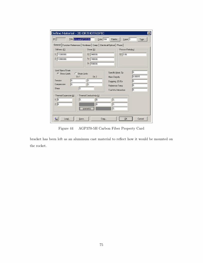
Figure 44 AGP370-5H Carbon Fiber Property Card
bracket has been left as an aluminum cast material to reflect how it would be mounted on
the rocket.
75

4.7.2 Modal Analysis. The first analysis conducted with the carbon-fiber model
was a modal analysis test whereby the natural frequencies associated with each mode were
calculated. The results from this test are displayed in Table 17. From the results, it appears
that the difference between the two materials is most noticable in the first two natural
frequencies. The carbon-fiber material has lower values associated with both the first and
second calcualted natural frequencies when compared to the aluminum model. This resulted
in a 29.9 and 18.8 percent difference, respectively. The second notable result from this data
table is the fact that the first and second natural frequency of the carbon-fiber model have
moved closer together by about 7 Hz.
Table 17 Carbon-Fiber Modal AnalysisMode Al A357-T6 (Hz) Carbon-Fiber (Hz) % Diff1 107.6 79.6 29.92 201.6 166.9 18.83 374.3 354.9 5.3
From these two aspects of the results, the following can be deduced. First, having
lower values of the natural frequencies means that future design teams could have lower
sampling rates for data collection with the strain gages. However, the lower values also
represent a less rigid structure that will probably result in higher specimen deflections
during the actual launch. This could possibly result in payload failure. Furthermore, the
fact that the first and second natural frequencies are closer together could result in further
negative repercussions for the payload. As far as flutter is concerned, this is not a enviable
feature. In most cases, you want to have the first bending and first torsion modes as far
away from each other as possible. Although the two frequencies have not come significantly
closer together, it is still something to take into account in the flutter analysis of future
experiments.
Interesting to note, it was originally anticipated that the carbon-fiber model would
have higher natural frequencies than the aluminum model. Essentially, it was thought that
by decreasing the mass and keeping the overall stiffness the same, the result would be higher
nautral frequencies. However, when dealing with carbon-fiber composites, it is important
to realize that there are many complex interactions in the material properties. The stiffness
76

of this material is a function of not only Young’s Modulus, but also of Poisson’s ratio and
direction. Ultimately, these complex contributing factors are believed to have caused this
unanticipated lower values of natural frequency. In future testing, it is highly recommended
to perform actual experimental tests to verify any and all finite element models before
arriving at any final conclusions.
Overall, the results of the carbon-fiber modal analysis indicate a less rigid structure
that is actually more prone to flutter. If this type of test specimen is going to be used in
future years, these types of concerns need to be addressed before an actual launch by means
of lab testing and material property analysis in order to obtain actual values of natural
frequencies, Young’s moduli, Poisson’s ratios, and shear moduli.
77

4.7.3 Strain Gage Predictions. The next set of tests conducted with the carbon-
fiber model analyze strain using the same flight profile and CFD predicted loads as the
aluminum model. For reference purposes, Tables 9 - 13 display the resultant forces and
loading configurations for each test case studied. Overall, this test was conducted in
anticipation of future test payloads in the FalconLAUNCH program.
Following the same setup and analysis as the aluminum model, strain contours of the
model were produced in FEMAP for a static analysis of the CFD predicted flight loads.
Figure 45 displays the contours produced for the same flight test points presented earlier in
Section 3.7.2 and in Table 4. Once again, the colors in the contour plots range from purple
indicating the lowest levels of strain to red indicating the highest levels of strain.
From these contour plots, it is once again evident that the highest strain concentrations
occur in the section joining the main wing and winglet portions of the test specimen. In
order to obtain specific strain readings, various nodes were studied in the pertinent sections
of the part. Table 18 was produced to display the calculated strain in the strain gage
locations of both the main wing and winglet sections and the readings at the highest strain
location.
Table 18 Carbon-Fiber Model Strain ReadingsAltitude(ft)/Mach Main Wing Gage Winglet Gage Highest Strain
5k/1.0 1.27E-03 1.35E-03 3.80E-039k/2.5 2.65E-03 2.81E-03 8.58E-0330k/4.5 1.66E-03 1.74E-03 5.46E-0360k/2.5 2.70E-04 2.86E-04 8.71E-04100k/1.0 1.84E-05 2.15E-05 5.76E-05
From these results, a few different conclusions can be drawn. Similar to the aluminum
model, the highest levels of strain occur during the acceleration of the rocket. Again, this
is due to the fact that the rocket is accelerating to high speeds in excess of Mach 2.0 at
low altitudes. The high pressure and density associated with these test points in the flight
profile cause this type of behavior. The second conclusion based on these results is somewhat
different than those of the aluminum model. Using the carbon-fiber material, it appears
78
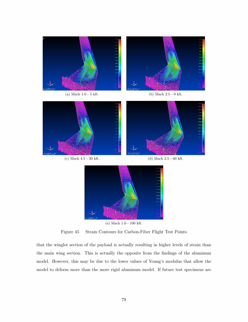
(a) Mach 1.0 - 5 kft. (b) Mach 2.5 - 9 kft.
(c) Mach 4.5 - 30 kft. (d) Mach 2.5 - 60 kft.
(e) Mach 1.0 - 100 kft.
Figure 45 Strain Contours for Carbon-Fiber Flight Test Points
that the winglet section of the payload is actually resulting in higher levels of strain than
the main wing section. This is actually the opposite from the findings of the aluminum
model. However, this may be due to the lower values of Young’s modulus that allow the
model to deform more than the more rigid aluminum model. If future test specimens are
79
to be comprised of carbon-fiber, then these results should be expanded upon to see the full
effect.
Another interesting note worth mentioning is the ultimate allowable strain for this
material. Using the longitudinal modulus and longitudinal tensile strength, the calculated
maximum allowable strain was found to be 0.0125. Comparing this maximum allowable
value to those calculated using the static lifting loads, it is evident that the part is not
expected to fail. The highest value of strain located in the section joining the main wing
and winglet section at Mach 2.5 at 9k feet was found to be 0.00858. This represents 68% of
the maximum allowable strain.
The last bit of information taken from this set of data once again follows the patterns
established by the aluminum model. Essentially, the strain readings lower dramatically as
the altitude increases. Looking at the main wing section and the area with the highest strain,
the strain drops off by two orders of magnitude. For a more visual display of the results
presented in Table 18, Figure 46 was created to plot the change in strain gage readings
versus the altitude of the rocket.
80

Figure 46 Plot of Carbon-Fiber Model Strain Results
81

4.7.4 Test Specimen Deflections. The next test conducted with the carbon-fiber
model was a deflection analysis. Again, using the same setup as described in Section 4.5.4,
FEMAP was used to analyze the static analysis and produce contour plots for each flight
test point shown in Figure 47. The contour colors range from purple representing the lowest
levels of deflection to red indicating the highest.
(a) Mach 1.0 - 5 kft. (b) Mach 2.5 - 9 kft.
(c) Mach 4.5 - 30 kft. (d) Mach 2.5 - 60 kft.
(e) Mach 1.0 - 100 kft.
Figure 47 Deflection Contours for Carbon-Fiber Flight Test Points
82
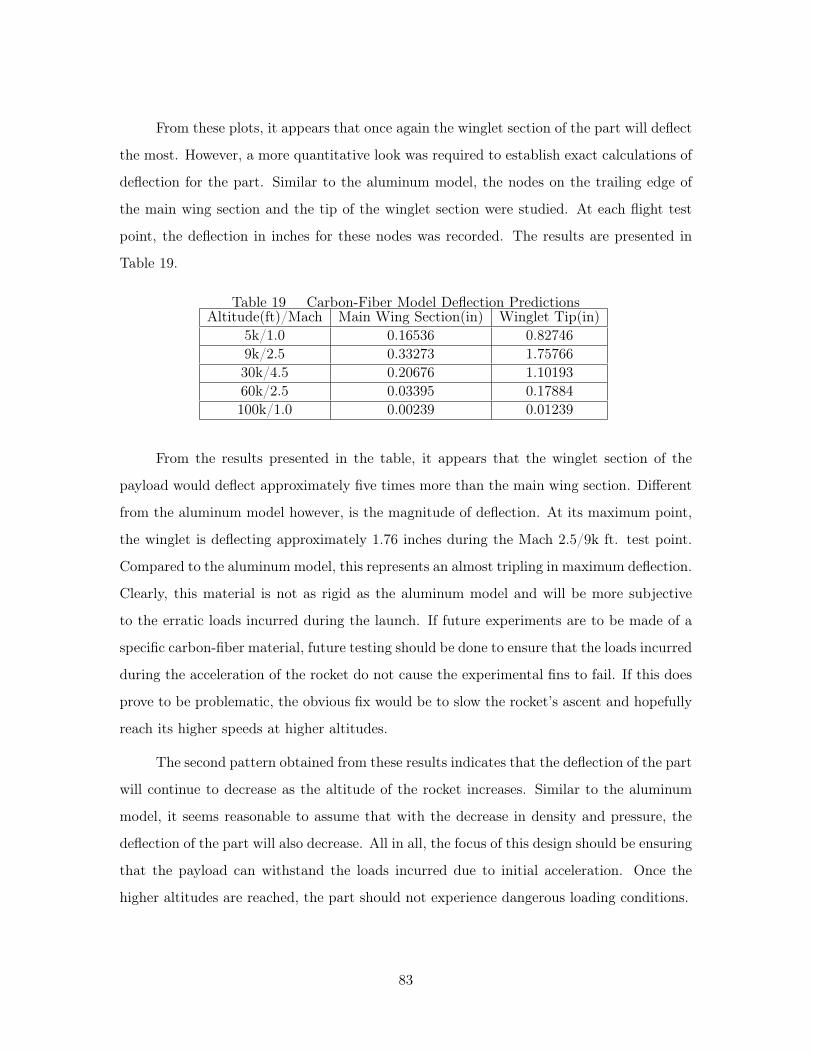
From these plots, it appears that once again the winglet section of the part will deflect
the most. However, a more quantitative look was required to establish exact calculations of
deflection for the part. Similar to the aluminum model, the nodes on the trailing edge of
the main wing section and the tip of the winglet section were studied. At each flight test
point, the deflection in inches for these nodes was recorded. The results are presented in
Table 19.
Table 19 Carbon-Fiber Model Deflection PredictionsAltitude(ft)/Mach Main Wing Section(in) Winglet Tip(in)
5k/1.0 0.16536 0.827469k/2.5 0.33273 1.7576630k/4.5 0.20676 1.1019360k/2.5 0.03395 0.17884100k/1.0 0.00239 0.01239
From the results presented in the table, it appears that the winglet section of the
payload would deflect approximately five times more than the main wing section. Different
from the aluminum model however, is the magnitude of deflection. At its maximum point,
the winglet is deflecting approximately 1.76 inches during the Mach 2.5/9k ft. test point.
Compared to the aluminum model, this represents an almost tripling in maximum deflection.
Clearly, this material is not as rigid as the aluminum model and will be more subjective
to the erratic loads incurred during the launch. If future experiments are to be made of a
specific carbon-fiber material, future testing should be done to ensure that the loads incurred
during the acceleration of the rocket do not cause the experimental fins to fail. If this does
prove to be problematic, the obvious fix would be to slow the rocket’s ascent and hopefully
reach its higher speeds at higher altitudes.
The second pattern obtained from these results indicates that the deflection of the part
will continue to decrease as the altitude of the rocket increases. Similar to the aluminum
model, it seems reasonable to assume that with the decrease in density and pressure, the
deflection of the part will also decrease. All in all, the focus of this design should be ensuring
that the payload can withstand the loads incurred due to initial acceleration. Once the
higher altitudes are reached, the part should not experience dangerous loading conditions.
83

As a final note, the results of Table 19 were graphed to visually show the deflection of
the carbon-fiber model as a function of increasing altitude. Figure 48 is able to display the
vast difference in deflection between the two parts of the payload. Although the differences
are great, the results are not unexpected. The less rigid carbon-fiber model was expected to
have a greater deflection than the aluminum part due to the results obtained in the modal
analysis in Section 4.7.2 which indicate a less rigid sturcture with lower values of natural
frequency. However, experimental tests should be conducted in the future to ensure that
the predicted loads do not cause the payload to fail.
Figure 48 Plot of Carbon-Fiber Model Deflection Results
4.8 Chapter Summary
In this chapter, the results for the various flight prediction tests were presented.
Starting with the flutter analysis conducted by the cadets at the Air Force Academy, this
84
analysis showed that the test specimen would not succomb to flutter. In order to perform
this test, the cadets sliced the geometry into two seperate pieces consisting of the main wing
and winglet sections. By conducting independent tests on each part, the flutter analysis
program, AeroFinSim showed that neither piece would reach the flutter velocity throughout
the entire flight profile.
By conducting a validation ping test, the calculated natural frequencies in FEMAP
were compared to experimentally obtained results. Overall, there was a high degree of
precision and accuracy associated with the first two natural frequencies with a maximum
difference of only 10% between the two. However, there was a discrepancy found with the
data obtained for the third natural frequency. The finite element model differs from the
experimental part by approximately 30%. Until a laser vibrometer test can be conducted,
the full justification for this disparity cannot be fully explained. However, after further
testing and possible tuning, this difference can hopefully be resolved. Overall, the successful
correlation of the first two natural frequencies indicate that there is a strong link between
both the finite element models and the actual cast part which allows for further flight
prediction testing.
The next set of test results presented were the strain gage and deflection data calcu-
lations done using FEMAP and the Al A357-T6 finite element model. In the strain gage
prediction tests, the results showed that the accleration of the rocket would result in the
largest strain readings culminating with maximum strain conditions during the Mach 2.5 /
9k feet altitude test point. Ultimately, the strain gages will record a considerable amount
of strain gage readings which will then be used to calculate vibrational data in order to
match the predicted modes and natural frequencies calculated with FEMAP. Furthermore,
the strain readings are predicted to drop off as the rocket reaches higher altitudes due to
the decrease in pressure and density. Table 14 in Section 4.5.3 presents the strain gage
readings for both the main wing and winglet sections of the test payload for static lifting
load deflections.
Next, the results for the static deflection test were presented for the Al A357-T6
model. Similar to the results in the strain gage tests, these results also show a maximum
deflection occurring during the acceleration of the rocket at the Mach 2.5 / 9k feet altitude
85

test point. During this test, the winglet section of the payload was found to deflect up to
six times more than the main wing section with a maximum deflection of approximately 0.6
inches. This analysis was conducted using the CFD predicted pressure loads at each of the
five test points analyzed throughout the flight profile of the rocket. More detailed results
are found in Table 15 of Section 4.5.4.
Pressing on, the effect of heating on the payload was then presented. In this test, the
Young’s Modulus of the aluminum model was decreased by increments of 5% from 10.5E6
psi to 8.4E6 psi representing a 20% reduction. The value of E was reduced to simulate the
effect heating has on an aluminum which resulted in a significant decrease in the natural
frequencies of the payload. By lowering the Young’s Modulus by 20%, the resulting natural
frequencies dropped by approximately 11%. Furthermore, it was determined that heating
the payload will also bring about the converging of the first bending and torsional mode
natural frequenceis which will effectively reduce the flutter speed. The results of this test
were presented in Table 16 of Section 4.6.
The last set of tests performed in this chapter dealt with the strain and deflection
calculations of a new carbon-fiber finite element model in order to anticipate the designs of
future FalconLAUNCH payloads. Using this new model, the same set of tests performed
on the aluminum model were conducted in order to highlight the differences between the
two materials. During the strain gage prediction tests, the results showed that the winglet
section of the payload was deflecting more than the main wing section. This result was
different from the aluminum models and is believed to be caused by the lower values of
Young’s Modulus resulting in a less rigid structure. Despite this difference, the same pattern
of decreasing strain readinsg with increasing altitude was observed. The full results of this
test are shown in Table 18 in Section 4.7.3.
The final carbon-fiber flight prediction test conducted was a static deflection test. In
this analysis, the results showed that once again the the wing tip section would deflect
more than the main wing section of the payload. However, the main difference between
the carbon-fiber model and the aluminum model was magnitude of deflection. The carbon-
fiber winglet was found to deflect three times more than the aluminum winglet resulting
in a maximum deflection of 1.76 inches during the Mach 2.5 / 9k feet altitude test case.
86

Ultimately, the less rigid carbon-fiber model will undergo a great deal of deflection. If
future models are to be wrapped in carbon-fiber, further testing should be done to assure
that failure will not occur during the flight profile of the rocket. These results are presented
in Table 19 of Section 4.7.4.
87

V. Conclusions and Recommendations for Future Work
5.1 Chapter Overview
The final chapter of this thesis will be broken into two different sections. The first
will serve as a conclusions section for the work done for this thesis and the next section will
discuss recommendations for future work with FalconLAUNCH and the ExFiT program.
5.2 Conclusions
In this thesis, the design and structural modeling of the payload for FalconLAUNCH
VIII was conducted in order to further the Air Force’s study of hypersonic flight and to
aid in the design of AFRL’s next space launch vehicle. Beginning with a historical look
at hypersonic research conducted by the Air Force, Chapter 2 of this paper was written to
provide a detailed look at past and present research attempts to conquer the technological
hurdles associated with hypersonic flight.
Since its inception, the Air Force has continually struggled to develop a hypersonic
cruise vehicle capable of becoming an operational weapons platform. This pursuit began
with the Dyna-Soar program and continued through DARPA’s Blackswift test bed. Unfor-
tunately, each time these goals came within arms-reach, the funding was scrapped. Looking
to other venues for hypersonic flight, the Air Force began funding a new project dedicated
to providing reliable and reusable means for space launch. In this light, the ExFiT program
began to take shape by studying different airfoil and wing tip configurations to be included
in the concept vehicle. In this research, one possible configuration was examined.
In order to study this wing and wingtip configuration, the model will be attached to
the Air Force Academy’s FalconLAUNCH sounding rocket in order to conduct a hypersonic
flight test. Strain gages and temperature thermistors have been attached to the main wing
and wingtip sections of the model in order to collect data throughout the flight of the rocket
and will be used to validate several finite element models used to conduct flight prediction
tests.
In Chapter 4 of this document, the validation of the finite element model and results
from the flight prediction tests were presented and included strain gage prediction and
88

payload deflection tests with the aluminummodel of this year’s test specimen. From Sections
4.5.3-4.5.4, it appears that the acceleration of the sounding rocket will result in the highest
readings for both strain and deflection of the part at the Mach 2.5 / 9k feet test point.
From here, the values decreased as rocket continued to gain altitude due to the decrease
in density and atmospheric pressure. The last test conducted with the aluminum model
pertained to the effect heating would have on the payload in terms of natural frequencies.
Essentially, while the part increases in temperature as will certainly happen as a result of
very rapid acceleration at low altitudes, the Young’s Modulus will decrease as a result[26].
By decreasing the value of E by 20%, the values of the first three natural frequencies dropped
by approximately 11% indicating a less rigid structure at high temperatures.
Next, a carbon-fiber finite element model was created in order to anticipate future
payloads for work in conjunction with the FalconLAUNCH program. Using this new model,
the same flight prediction tests were conducted with some similar results. Following the
patterns of the aluminum model, the highest values for strain and payload deflection
occurred during the Mach 2.5 / 9k feet test case. However, the differences between the
two models dealt with magnitude of both strain and deflection. In this scenario, the less
rigid carbon-fiber model had higher values of both strain and winglet deflection. According
to the results presented in Sections 4.7.3-4.7.4, the carbon-fiber model will have three times
more strain and deflection than the aluminum model. If this type of material is to be used
in future research pursuits, further testing should be conducted to ensure that the part will
not fail during the intended flight profile.
Overall, this thesis should be viewed as a setup for future experiments and used to
validate the finite element models created for flight prediction purposes. The intent of this
paper was to build the foundation for future research and test specimen designs. At the
very least, the procedure for creating and running the flight prediction tests on the finite
element models can be used for future ExFiT projects. Although this section concludes the
discussion of the research completed for this year’s experiment, the following section will
offer detailed guidelines for further endeavors in the ExFiT program.
89

5.3 Recommendations for Future FalconLAUNCH and AFRL FAST Work
The final section of this paper will discuss several key aspects for inclusion in future
work with the ExFiT program in conjuction with the Air Force Academy’s FalconLAUNCH
program. The first topic discussed deals with the flutter analysis conducted this year and
offers suggestions for successive studies to come. Next, the topic of enhancing the finite
element models to include a dynamic loading is discussed in order to simulate the rocket’s
vibration during the launch. Following this, the topic of FEM validation through the use
of finite element model tuning and actual static loading tests are discussed. After this,
recommendations are offered regarding the design of future payloads for the rocket to include
sensor locations, material selection, heating profiles, shape, and location of the model.
Finally, this chapter will conclude with a discussion regarding the scaling of the results
from this thesis to full-size in order to be relavent to the FAST concept vehicle.
5.3.1 Future Flutter Prediction Tests. Although the flutter analysis presented in
Chapter 4 of this report offered favorable results, the methodology can be improved upon to
increase the accuracy of the findings. For example, if another wing and wingtip geometry is
to be used, then a few steps can be taken to enhance the viability of the results found using
AeroFinSim. Looking at the main wing section first, it is suggested to place an addional
mass concentration at the tip of the section to model the wingtip that will be connected
there in reality. Just by approximating this value, the analysis will reflect a more accurate
scenario to be analyzed.
The next big suggestion would be to consider remodeling the mount of the wingtip
section to simulate a less rigid mount. For example, by placing linear or torsional springs
at the mount, the behavior of the main wing section can be somewhat modeled within
the flutter program. With iterative runs, the behavior of the main wing section could be
decently approximated. Overall, the use of AeroFinSim is limited to its original design:
rocket fins. However, with these suggested ways to manipulate this program, more accurate
results can then be obtained.
Aside from using the AeroFinSim program, another flutter program could be used for
future experiments in order to add a significant amount of accuracy to the calculations.
90

For example, ZONA Technology’s ZAERO program uses a P-K method, referred to as the
g method in the program, that calculates the flutter velocity for a user input geometry.
Breaking away from the fin geometry required by AeroFinSim, ZAERO allows the user to
create a seperate model of the structure before being read into ZAERO. In this case, the
finite element models created in this thesis could be used if similar geometries are considered
in future experiments. Using the NX Nastran analysis software included in FEMAP, the
results from the modal analysis of the model could then be read into ZAERO along with
the other variables to include altitude and velocity information from the flight profile of the
rocket [29]. From here, an accurate flutter study could be conducted that is reflective of the
entire test geometry as a whole that more closely resembles the actual rocket payload.
Looking at other flutter studies conducted for the Academy in previous years, J.
Simmons created a flutter optimization tool to use for rocket fin designs [18]. In his
analysis, Simmons originally planned on using ZAERO for his calculations, but decided
against it due to the iterations he would have to perform for various changes in design to
the fins in his optimization process. Specifically, changes in chord, span, or thickness meant
adjusting both the ZAERO models and the finite element models and conducting seperate
grid independence tests to ensure the validity of the results. However, in the circumstance
that a test specimen has already been designed, ZAERO could be used to ensure that the
part will not flutter.
5.3.2 Rocket Vibration and Dynamic Loading for FEMs. The next topic discussed
for future research deals with the creation and usage of finite element models for flight
prediction studies. For this thesis, a static analysis of the CFD calculated flight pressure
loads was used to predict static deflections and frequencies. However, for future work, these
models should be expanded upon to include a variety of items to enhance the fidelity of the
models. To start, the actual behavior of the rocket should be considered seeing as it is not
a rigidly fixed body in flight. Furthermore, these transient loads during acceleration could
very well exceed steady state predicted loads. In order to model the rocket’s vibration, one
possible suggestion would be to include linear and torsional springs attached to the model
at the mounting bracket. The user could then tune the rigidity of the springs to correlate
91

the data collected during the launch. This type of analysis must be done first in order
to compare the data recorded from the rocket launch to the results found in Chapter 4.
Essentially, the data will have to be filtered in order to take out the transient vibrations
of the rocket. Simply put, the analysis conducted in Chatper 4 was purely static and did
not include the transient behavior of the actual vehicle. Therefore, one of the first steps in
future work will be to post-process the data collected from FalconLAUNCH VIII to compare
with the finite element tests conducted as flight prediction experiments.
Another suggestion to improve FEM accuracy would be to incorporate a dynamic
loading analysis into the flight prediction experiments. This time-varient analysis could
actually be used to expand upon the test points used for this research paper. One approach
would be to vary the pressure loads on the test specimen in time in conjunction with the
flight of the actual rocket to encompass more of the flight profile. By modeling both the
transient nature of the rocket as well as adding a time-varying loading configuration, the
fidelity of the results could be further enhanced. This increase in accuracy will help future
endeavors in payload design.
5.3.3 Validating and Tuning the FEMs Created for Flight Prediction. Originally,
it was expected that AFIT would have received two of the test specimens in early December
of 2009 for physical testing purposes. However, due to setbacks in production, they were
not received until late February of 2010. With the time remaining, only a ping test could
be conducted and included in this body of work as a way to validate the finite element
models. However, from the results obtained in Chapter 4, there are a few more tests that
are recommended for full finite element model validation.
The first suggested test would be a laser vibrometer scan to conclusively determine
both natural frequencies and mode shapes of the cast part. From here, the disparity
regarding the third natural frequency could be more fully examined and possibly resolved.
With the laser scan, the shape of this mysterious mode could be compared to the results
obtained in FEMAP as a way to track down the reason for the difference in results.
Furthermore, model tuning is also recommended as a way to further bring the results
between the computational and experimental results together. In this procedure, the
92

Young’s Modulus of the finite element model is iteratively changed in order to reflect the
results obtained experimentally. In this light, the finite element models could be validated
to more fully capture the behavior of the part.
The next validation test planned for the part was intended to compare deflection data
between the actual part and FEMAP using the static loads projected by the CFD analysis.
It had been hypothesized that by hanging the part upside down and attaching weights or
sandbags to the main wing section of the test specimen, sensors could have been used to
verify the static deflections on that specific section. This test may have taken a bit more
time, but would have validated the performance of the part using 2Lt Switzer’s calculated
pressure loads.
Although these tests were not able to be completed in time, the ultimate FEM
validation test is forthcoming in the launch later this Spring. After filtering the transient
behavior of the rocket, the results of the recorded data can be directly compared to the flight
prediction tests conducted in Chapter 4. If the two sets of data are equivalent, than it can
be safely assumed that the FEMs are accurate and can be used in future research pursuits.
Otherwise, hopefully the two projected tests above can find the discrepancies between the
models and the physical specimens and the differences can be corrected.
5.3.4 Sensor Locations for Future Experiments. In this subsection, the location
of the sensors for future experiments will be discussed. If the current design for Falcon-
LAUNCH VIII is used again, then it will prove beneficial to analyze the mode shapes of
the current test specimen to determine where to place next year’s gages. Optimally, strain
gages should be placed in the area of the test specimen that will deform the most and that
will avoid the node lines associated with each mode. For the current design, Figure 49 has
been presented to display the shapes of the first three modes to be captured in this year’s
launch. These results were obtained during the modal analysis conducted in Chapter 3.
Looking at the resulting mode shapes for the first three natural frequencies, two
seperate conclusions can be drawn. First, it appears that the trailing edge of the main
wing section closest to the joining of the main wing and winglet sections should be the new
target area for the strain gages. This conclusion was reached based on the observation that
93

(a) Un-Deformed Model (b) First Mode Shape
(c) Second Mode Shape (d) Third Mode Shape
Figure 49 First Three Natural Mode Shapes of the FEM
this targeted region is undergoing a significant amount of deflection for each resulting mode
shape. Similarly, this region of the wing does not fall on a node line for any of the targeted
modes. Second, it appears that the location selected for the winglet was appropriate and
that no significant changes should be made to this location. The location pre-selected for
this year is deflecting with each natural frequency and there does not appear to be an area
that performs any better than the location selected. Figure 50 shows the targeted strain
gage region for the main wing section of future experiments of this shape.
In general, the location of strain gages for future experiments should follow a similar
process of analyzing mode shapes to determine test locations. If a different geometry is
used, a new finite element model should be generated and analyzed. From the resultant
modal anlaysis, the location of the strain gages should be determined up front rather than
after a design has been decided upon as was done for this experiment.
94

Figure 50 Location of Future Strain Gage Placement
5.3.5 Material Selection and Heating Profile Studies. FalconLAUNCH VIII in-
cluded a test specimen cast from Aluminum A357-T6 attached to its body. For future
experiments, however, other materials should be discussed to more closely resemble the
concept FAST vehicle. Therefore, a future experiment should include a carbon-fiber test
specimen. Seeing as the FAST vehicle is to be composed of carbon-fiber materials, it would
be beneficial to at least include a patch of this material to one of the experiments. With
any luck, the design team could wrap an entire test specimen in a carbon-fiber composite
like the model analyzed in Chapter 4. With this type of arrangement, the inclusion of
thermistors and strain gages could then be used to provide necessary heating profiles and
deflection data during the launch which would be very beneficial to AFRL and the FAST
program.
Looking at the results from the heating study conducted with the aluminum model
in Section 4.6, it was evident that the first and second natural frequencies grew closer
together as the temperature increased and the Young’s Modulus decreased. In future work
95

with carbon-fiber models, a more complex heating study should be conducted to establish
the general effect of heating on future test specimens and its correlation to the specimen’s
flutter. After testing and establishing a heating profile across the wing in successive launches,
hopefully future research can find a material that is able to best withstand the converging of
the first two natural frequencies and manage the large amount of heat generated from flight
at hypersonic speeds. If necessary, new airoils should also be considered in order to achieve
these goals. Overall, future heating studies with carbon-fiber test specimens should receive
a large portion of research time due to its direct correlation to FAST’s concept vehicle.
5.3.6 Shape and Location of Next Year’s Experiment. Ultimately, the size and
placement of next year’s experiment will depend heavily on the success or failure of Fal-
conLAUNCH VIII. If the rocket can ensure data collection and stable flight throughout its
profile, then there really should not be a lot of change in successive designs. From this point,
the next step in design would ultimately come from changes in material and geometry.
However, if the rocket flight becomes unstable or erratic due to the inclusion of the two
test specimens, then changes in the shape and placement of future experimental payloads
must be made. First, a less complex design should be analyzed. For example, a carbon-fiber
wrap of a less complex test specimen, such as a wing geometry, would still prove beneficial
to FAST. In this setup, a heating profile of a carbon-fiber wrapped wing would directly aid
the design of the concept RBS. By conducting this type of experiment, the wing section
would still undergo a hypersonic flight profile and as a benefit, the carbon-fiber wrap could
also be tested.
If the inclusion of a simple wing shape is still deemed too risky, then a vertical stabilizer
wrapped in carbon-fiber would still prove useful to the research done with FAST. By using
a set of thermistors, a decent heating profile could still be tested and stable flight would be
ensured by resorting to the design of FalconLAUNCH VII.
As far as location is concerned, the rear of the rocket would still provide the best flight
stability. As determined early in the design process for FalconLAUNCH VIII, anything
placed on the nose cone of the rocket would just create more problems up front than
necessary. Ultimately, this configuration would take up precious time that the cadets do
96

not have. Unless proven otherwise, future payloads should remain at the rear end of the
rocket. This locale works to the benefit of both the designers and the customers hoping for
reliable data collection.
Overall, the success or failure of the upcoming launch will dictate further design
changes to the flight payload. If the launch is successful, new materials should be discussed
without great change to design and location of the experiment. However, if the launch is
unsuccessful, future tests will have to be re-designed. The two possible options discussed
here include reducing the complexity of the test specimen to a wing shape, or going back
to the regular vertical stabilizers composed of a carbon-fiber composite. Either way, the
location of the payload should remain in the rear of the rocket with the stabilizers.
5.3.7 Scaling Results to a Full-Size Vehicle. This subsection will discuss some of
the most important work still to be done for the development of the FAST concept vehicle.
Basically, besides the testing and setup of future FalconLAUNCH experiments, necessary
research must be done to scale the results from this experiment to be relevant to the actual
FAST vehicle. In this experiment, predicted loads have been generated using CFD analysis
and finite element programs of a 1/10 scale model. Aerodynamic and aeroelastic scaling
must still be done to take the results obtained in this experiment and make them useful to
the FAST vehicle in its entirety.
It is important to note, however, that this may prove to be a daunting task. Aeroelastic
and aerodynamic scaling are not perfect, and ultimately, not everything can be accurately
scaled to represent the full-size vehicle. Therefore, it was intented that this research be used
as a foundation upon which future work can build. By outlining the overall design of the
experiment and by building the necessary FEMs, the next student to continue this work
could start from where this research leaves off and hopefully begin to scale the results or
make the minor changes dictated to the design of future experiments to further the work
being done for FASTs RBS.
97

Bibliography
1. Hellman, B., McKee, K., Street, M., and Remillard, C., 2009. “Advancing ORSTechnologies and Capabilities with a Space Tourist Suborbital Vehicle.” In AIAASPACE 2009 Conference and Exposition.
2. Dyna-Soar Mock Up. Internet picture accessed 1 Jan. 2010 fromhttp://en.wikipedia.org/wiki/X-20_Dyna-Soar.
3. Dyna-Soar With Booster. Internet picture accessed 1 Jan. 2010 fromhttp://www.astronautix.com/craft/dynasoar.htm.
4. NASA’s M2-F1 Lifting Body Vehicle. Internet picture accessed 5 Jan. 2010 fromhttp://www.nasa.gov/topics/history/M2_F1.html.
5. NASA’s HL-10 Lifting Body Vehicle. Internet picture accessed 5 Jan. 2010 fromhttp://www.dfrc.nasa.gov/Gallery/photo/HL-10/Medium/ECN-2064.jpg.
6. Blackswift Model. Internet picture accessed 2 Jan. 2010 fromhttp://www.flightglobal.com/blogs/the-dewline/blackswift.jpg.
7. Artist Rendering of Blackswift. Internet picture accessed 2 Jan. 2010 fromhttp://www.flightglobal.com/assets/getAsset.aspx?ItemID=25618.
8. HIFiRE 0 Launch on May 7, 2009. Internet picture accessed 15 Jan. 2010 fromhttp://www.uq.edu.au/hypersonics/?page=19501.
9. XCOR Lynx Vehicle. Internet picture accessed 2 Jan. 2010 fromhttp://www.xcor.com/press-releases/2008/images/lynx_suborbital_ascent.
10. Houchin, R. F., 2006. US Hypersonic Research and Development - The Rise and Fallof Dyna-Soar (1944-1963), First ed. Routledge, 270 Madison Avenue, New York, NY10016.
11. McMillan, B. Review of the Air Force Space Research and development Program. Letterto Secretary of Defense McNamara, June 1963.
12. McNamara, R. Cancellation of the X-20 Program. News Brief - Washington, D.C.,December 1963.
13. Kempel, R., Painter, W., and Thompson, M., 1994. Developing and Flight Testing theHL-10 Lifting Body: A Precursor to the Space Shuttle. Reference Publication 1332,NASA, April.
14. DARPA FALCON(Force Application and Launch from CONUS)Technology Demonstration Program Fact Sheet. On the WWW, athttp://www.darpa.mil/news/2003/falcon_fs.pdf, November 2003 PDF file.
15. DARPA Falcon Technology Demonstration Program HTV-3X Blackswift Test Bed. Onthe WWW, at http://www.darpa.mil/Docs/Falcon-Blackswift%20FS%20Oct08.pdf,October 2008 PDF file.
98

16. Dolvin, D. J., 2008. “Hypersonic International Flight Research and Experimentation(HIFiRE) Fundatmental Sciences and Technology Development Strategy.” In 15thAIAA/AAAF International Conference: Space Planes and Hypersonic Systems andTechnologies.
17. Odam, J., Paull, A., Alesi, H., Hunt, D., Paull, R., and Pietsch, R., 2009. “HIFiRE0 Flight Test Data.” In 16th AIAA/DLR/DGLR International Space Planes andHypersonic Systems and Technologies Conference.
18. Simmons, J. R., 2009. “Aeroelastic Optimization of Sounding Rocket Fins.” MS Thesis,Air Force Institute of Technology Graduate School of Engineering and Management,Wright-Patterson AFB, OH 45431. AFIT/GSS/ENY/09-J02.
19. Nasa Space Vehicle Design Criteria: Flutter, Buzz, and Divergence. Technical ReportNASA SP 8003, NASA, 1964.
20. Martin, D., 1958. Summary of flutter experiences as a guide to the preliminary designof lifting surfaces on missiles. Technical Report NACA TN 4197, NACA.
21. Hodges, D., and Pierce, A., 2002. An Introduction to Structural Dynamics andAeroelasticity John Wiley & Sons, Inc., 605 Third Avenue, New York, NY 10158.
22. AeroRocket, 2006. AeroFinSim v4.0 User Manual, latest ed. See also URLhttp://www.aerorocket.com/finsim.html.
23. Switzer, B. P., 2010. “CFD Analysis of Experimental Wing and Winglet forFalconLAUNCH VIII and the ExFiT Program.” MS Thesis, Air Force Institute ofTechnology Graduate School of Engineering and Management, Wright-Patterson AFB,OH 45431. AFIT/GAE/ENY/10-M25.
24. Prototype Casting Inc.. Internet information and homepage accessed 27 Jan. 2010 fromhttp://www.protcast.com/.
25. Matweb-Material Property Data. Internet information accessed 15 Dec. 2009 fromhttp://www.matweb.com/index.aspx.
26. Callister, W., 2007. Materials Science and Engineering - an Introduction, Seventh ed.John Wiley & Sons, Inc., 605 Third Avenue, New York, NY 10158.
27. Pilkey, W., 1994. Formulas for Stress, Strain, and Structural Matrices John Wiley &Sons, Inc., 605 Third Avenue, New York, NY 10158.
28. Daniel, I., and Ishai, O., 2006. Engineering Mechanics of Composite Materials,Second ed. Oxford University Press, Inc., 198 Madison Avenue, New York, NY 10016.
29. ZAERO User Manual. Zona Technology, Scottsdale, AZ 2007.
99

Vita
Second Lieutenant Michael Vinacco graduated from Poquoson High School in
Virginia in 2004 and pursued an undergraduate degree at the Virginia Military Institute.
Graduating with a Bachelor of Science in Mechanical Engineering, he was commissioned
into the US Air Force in May of 2008. As his first assignment, he was selected to attend
AFIT and arrived in August of the same year. During his time at AFIT, Lt Vinacco was
married to his wife in June of 2009 and went on to complete the Aeronautical Engineering
program in March 2010. Lt Vinacco has since been assigned to the 538th Air Sustainment
Depot located at Hill Air Force Base to begin working in the A-10 directorate in May of
2010. In June of 2010, Lt Vinacco and his wife will be expecting the birth of the couple’s
first child.
100
REPORT DOCUMENTATION PAGE Form Approved OMB No. 074-0188
The public reporting burden for this collection of information is estimated to average 1 hour per response, including the time for reviewing instructions, searching existing data sources, gathering and maintaining the data needed, and completing and reviewing the collection of information. Send comments regarding this burden estimate or any other aspect of the collection of information, including suggestions for reducing this burden to Department of Defense, Washington Headquarters Services, Directorate for Information Operations and Reports (0704-0188), 1215 Jefferson Davis Highway, Suite 1204, Arlington, VA 22202-4302. Respondents should be aware that notwithstanding any other provision of law, no person shall be subject to an penalty for failing to comply with a collection of information if it does not display a currently valid OMB control number. PLEASE DO NOT RETURN YOUR FORM TO THE ABOVE ADDRESS. 1. REPORT DATE
25-03-2010 2. REPORT TYPE
Master’s Thesis 3. DATES COVERED (From – To)
Sept 2008 – Mar 2010 4. TITLE AND SUBTITLE ExFiT Flight Design and Structural Modeling for FalconLAUNCH VIII Sounding Rocket
5a. CONTRACT NUMBER
5b. GRANT NUMBER 5c. PROGRAM ELEMENT NUMBER
6. AUTHOR(S) Vinacco, Michael J., 2LT, USAF
5d. PROJECT NUMBER 5e. TASK NUMBER
5f. WORK UNIT NUMBER
7. PERFORMING ORGANIZATION NAMES(S) AND ADDRESS(S) Air Force Institute of Technology Graduate School of Engineering and Management (AFIT/ENY) 2950 Hobson Way, Building 640 WPAFB OH 45433-8865
8. PERFORMING ORGANIZATION REPORT NUMBER AFIT/GAE/ENY/10-M27
9. SPONSORING/MONITORING AGENCY NAME(S) AND ADDRESS(ES) Mr. Barry Hellman Air Force Research Laboratory Air Vehicles Directorate 2130 8TH ST B20045 R261 Wright-Patterson AFB, OH 45433
10. SPONSOR/MONITOR’S ACRONYM(S) 11. SPONSOR/MONITOR’S REPORT NUMBER(S)
12. DISTRIBUTION/AVAILABILITY STATEMENT APPROVED FOR PUBLIC RELEASE; DISTRIBUTION UNLIMITED.
13. SUPPLEMENTARY NOTES
14. ABSTRACT This research effort furthers the Air Force's study of reusable launch vehicles and hypersonic airfoils by conducting a hypersonic flight test using the US Air Force Academy's FalconLAUNCH VIII sounding rocket. In this study, two experimental fin tips were designed and attached to the sounding rocket in place of two stabilizer fins in order to collect data throughout the rocket's hypersonic flight profile. The desire to research, study, and test experimental fin tips was driven by the Air Force Research Laboratory's Future responsive Access to Space Technologies (FAST) program and their desire to include vertical stabilizers on the wing tips of reusable launch vehicles (RLVs). In this research study, finite element models of the experimental fin tips were developed and used to predict the flight data collected by the strain and temperature gages attached to the test specimen. The results of these flight prediction tests showed that the test specimen will undergo the greatest deflection and strain during the acceleration of the rocket. Maximum deflection and strain gage readings were obtained at a speed of Mach 2.5 at an altitude of 9k feet. Ultimately, the payload will undergo a maximum deflection of 0.6 inches at the fin tip and a maximum strain gage reading of 0.00122 on the main wing section of the payload. 15. SUBJECT TERMS hypersonic flight test; reusable launch vehicles; experimental fin tips; FalconLAUNCH;
16. SECURITY CLASSIFICATION OF:
17. LIMITATION OF ABSTRACT
UU
18. NUMBER OF PAGES
114
19a. NAME OF RESPONSIBLE PERSON Dr. Jonathan T. Black, AFIT/ENY
a. REPORT
U
b. ABSTRACT
U
c. THIS PAGE
U
19b. TELEPHONE NUMBER (Include area code) (937) 785-3636 ext 4578
Standard Form 298 (Rev. 8-98) Prescribed by ANSI Std. Z39-18