Paper No. 5809 - Ohio University

ComparisonofModelPredictionsandFieldData–theCaseofTopoftheLineCorrosion

Ussama Kaewpradap, Marc Singer, Srdjan Nesic, Suchada Punpruk2

Institute for Corrosion and Multiphase Technology, Department of Chemical and Biomolecular Engineering, Ohio University, Athens, OH 45701, USA

2PTT Exploration and Production, Bangkok, 10900, Thailand

ABSTRACT

Top of the Line Corrosion (TLC) is a specific type of corrosion that happens due to internal water condensation in wet gas lines. It is a serious concern for the oil and gas industry and has been the cause of numerous pipeline failures. Many research projects have been executed with the aim to better understand the mechanisms and to develop accurate predictive models of TLC. Irrespective of their complexity, most of the models are based on laboratory experimental data. This makes it important, even in the case of most advanced models to compare and validate the model’s predictions by using field data. Data collected from sweet wet gas lines that experienced TLC issues were analyzed, processed, and then used as an input for a mechanistic TLC predictive model to simulate the evolution of temperature, pressure, water condensation rates and TLC rate along the pipeline. The simulation results were then compared with in-line inspection (ILI) data. Challenges were encountered in the analysis of the field data due to their incompleteness, inaccuracy and variability, as well as with processing of the ILI data. A coherent methodology for comparison with model prediction results was developed and described.

KEY WORDS: Top of the line corrosion (TLC), modeling, field data, magnetic flux leakage (MFL) data

INTRODUCTION

Top of the line corrosion (TLC) is associated with numerous pipeline failures and, is a growing concern for the oil and gas industry1-5. TLC is encountered under water condensing conditions in wet gas pipelines, operated in a stratified flow regime at low gas velocity. Water along with the light hydrocarbons condenses on the top and the sides of the inner pipeline surface due to the temperature difference between the external and internal pipeline environments. Corrosive species, such as carbon dioxide (CO2), hydrogen sulfide (H2S) and volatile organic acids are also present in this condensed water, making it very corrosive11,12. TLC has been intensely studied over the past decade with the aim to better understand the underlying corrosion mechanism and to develop accurate prediction models and successful

1

Paper No.

5809

Government work published by NACE International with permission of the author(s).The material presented and the views expressed in this paper are solely those of the author(s) and are not necessarily endorsed by the Association.

mitigation techniques6-14. A variety of corrosion prediction models has been proposed with varying degrees of complexity and sophistication. In all cases, there is a wide gap between development of corrosion models in academic and research institutions and their application in the field. The corrosion mechanisms implemented in the models are based on laboratory investigations6-10 and researchers are often hesitant to use field data for validation due to their incompleteness, inherent complexity and perceived lack of accuracy. On the other hand, field engineers are also reluctant to use models for corrosion risk assessment due to a level of mistrust in the model’s ability to predict corrosion in complex field conditions and a misunderstanding of model’s validity and limitations. Therefore, field engineers often rely exclusively on inspection data and past experience. In order to bridge this gap, the performances of any model - in this case, a mechanistic TLC prediction model - need to be validated with field experiences involving actual pipeline TLC failures. In 2010, Gunaltun et al. presented a first attempt to compare TLC prediction model results with field data measurements. In theory, a top of the line environment constitutes a prime candidate for comparing field measurement and model predictions, as the chemistry of condensed water is relatively simple and is not altered by the complex brine composition encountered in the bulk liquid phase. However, some considerable challenges still exist when comparing uniform corrosion model predictions to ILI data, which often represent defects in the form of small pits. However, TLC defects, at least in sweet environments, have been reported to be made of many large “mesa attack type” features, which are governed by uniform corrosion mechanisms15. In practice, incomplete and inaccurate field data often still make this exercise very difficult16. While the blame is too often placed on ineffective predictive models, few efforts have been made to develop a method that is truly able to effectively use actual field data. A purely mathematical/statistical approach cannot be used uncritically to process large volumes of field data, as convenient and tempting as that may be. This would lead to inclusion of poor quality data, inaccurate data and ultimately even nonsensical data into the analysis, rendering it all but useless. In any case, the model predictions cannot be expected to be of better quality than the input field data which are used for their validation. Examples of some typical mistakes made when processing field data that should be avoided are listed below:

Decades of production history should not be averaged to get one single set of input data (i.e. one average pressure, one average temperature, one average gas flow rate …). Production data fluctuate far too often for a simple, averaged value to have any meaning.

Often, too much confidence is placed in In Line Inspection (ILI) data. It is understood that these measurements are often the only tools available to assess corrosion during operation, but the inaccuracy of such tools (e.g. those using the magnetic flux leakage, ultrasonic method) must be accounted for. For example, a comparison between two consecutive ILI runs should be made only if the inspection and analysis are performed using the same tool and the same mathematical algorithm for analysis. If not, this exercise cannot be expected to produce meaningful data for validation of prediction models.

As a result, this first attempt to compare field data and model predictions16 served more to highlight the gaps in understanding and the difficulties in interpreting the results, than to provide valuable insights into the validity of TLC mechanisms and predictions made by the model. Consequently, a new methodology is proposed here in order to address these issues. It aims at developing a more representative set of input parameters (based on production data) and output parameters (based on ILI data), with the main objective being to identify gaps in the modeling approach. In the present work, the mechanistic TLC model TOPCORP(†) (referred to as the “model” in the following text) developed by the Institute of Corrosion and Multiphase Technology (ICMT)(1) at Ohio University was used, and its capabilities were validated

† Trade name (1) Institute for Corrosion and Multiphase Technology (ICMT), 342 West State Street, Athens Ohio 45701.

2


against subsea line data from an offshore gas field in the Gulf of Thailand that has been in operation since 1992. A similar effort has been already published by the authors17 presenting very much the same methodology. This paper adds new information about the field and an improved discussion of the results.

A TOP OF THE LINE PREDICTION MODEL

The theory and implementation behind the TLC model used in the current study was developed originally by Zhang et al.9 This model provides a fully mechanistic description of the TLC process. The three major phenomena covered by this model are: Dropwise condensation, used for condensation rate calculation based on heat and mass transfer theory Chemistry of the condensed water, developed from thermodynamic arguments by using chemical

equilibria Corrosion, where the TLC rate was predicted based on the kinetics of the electrochemical reactions

The model was adapted to running line simulations where, in order to obtain predictions along a pipeline, only pipeline inlet parameters and pipeline physical characteristics are required, as listed in Table 1:

Table 1: List of input parameters to the model

Parameter name Inlet temperature and total pressure

CO2, H2S gas content Brine composition (especially bulk water pH and organic acid content)

Gas, water and oil/condensate flow rate in standard conditions Pipeline diameter, roughness, section length, inclination

Thermal insulation (coating concrete …) Burial ratio and depth

The main output parameters are listed in Table 2:

Table 2: List of model’s output parameters

Parameter name pH and chemistry of the condensed water along the line

Water condensation rate along the line Steady state uniform top of the line corrosion rate along the line

The effect of many important factors on TLC, such as gas temperature, CO2 partial pressure, gas velocity, condensation rate and acetic acid concentration were accounted for in the model9. However, the effect of oil/water co-condensation was not taken into account, as the research on this topic was still ongoing at the time this study was performed. Since then, recent experimental work18 has shown that the condensation of light hydrocarbons does not seem to prevent liquid water from reaching the hydrophilic steel surface. It should be noted that the experimental work was performed with only one hydrocarbon (heptane) and that the conclusions may differ if other, heavier hydrocarbons are considered. However, the mere fact that so many wet gas lines suffer extensively for TLC is a good indication that one should not rely solely on the co-condensation of hydrocarbons for corrosion mitigation.

A METHODOLOGY FOR COMPARING MODEL PREDICTIONS WITH FIELD DATA

There are many difficulties that need to be overcome when directly comparing ILI data and model predictions. These problems can be classified into three main groups as follows:

Issues related to the accuracy of field data

3


- Availability, completeness and accuracy of production data. - Significant variations in production data over time. - Availability and accuracy of topographic data, environmental conditions and pipeline properties.

The mechanistic model used in this study is only sensitive to a set of basic input parameters such as production rates, temperature, pressure, etc. These input parameters can vary tremendously over the course of a field’s production life. The level of uncertainty and inaccuracy related to these data can be significant and represents the most difficult challenge in the analysis. In addition, the topography (pipeline inclination), bathymetry (pipeline burial) and information about the outside environment (on/offshore, outside temperature) are essential for calculation of the condensation rate and TLC corrosion evaluation.

Issues related to the model predictions

- Which model prediction data should be compared with the ILI data? - How to incorporate variations in production data over time into the prediction? - How to reflect the change in the conditions and the TLC rate along the pipeline in the model?

Even though the model has been developed to predict transient corrosion, it suggests that a uniform steady state TLC rate is typically obtained in a matter of weeks or months19. While production parameters vary continuously, these variations are also only significant on a monthly basis. It is therefore more appropriate that the model’s steady state corrosion rates are compared to the wall thickness loss data obtained from ILI inspections, as long as the main corrosion mechanism is uniform (large mesa type features) and not pitting (small pits influenced by galvanic coupling). Production data are also often taken on a daily basis, but it is not practical to simulate every single production data entry. In order to address this issue, longer time periods showing similarities in terms of input production parameters can be selected, and time-averaged input parameters can be defined for each time period, and then fed into the model. Consequently, a thorough analysis of the production data needs to be conducted, leading to the identification of these time periods. Changes in operational parameters over time can then be accounted for, provided that a thoughtful identification of the time periods has been performed.

Issues related to the analysis of ILI data

- How to take into account the inherent inaccuracy of TLC feature sizing? - Should the size or spatial distribution of the TLC features be considered in addition to the

maximum depth of attack? - What is the best approach to compare model predictions with complex ILI data?

Magnetic flux leakage testing (MFL) is probably the most widely-used, non-destructive testing (NDT) tool in the oil and gas industry for inspecting pipeline structures. It is crucial to point out that MFL does not directly measure wall thickness loss. Rather, deviations in the magnetic fluxes are translated into defect sizing by proprietary algorithms. These algorithms very from vendor to vendor, and also vary across different tools. In addition, the algorithms are continuously updated and calibrated. As a result not all ILI data are of the same accuracy/quality, although a typical accuracy on the order of 10 to 20% of the nominal wall thickness is often claimed20. Typically, ILI results obtained with the MFL technique are presented in terms of a list of defects along the pipeline. Each defect is associated with a specific circumferential location and a corresponding wall thickness loss. Additional information relating to the merger of small defects into clusters can also be available. The presence of clusters is typical of a TLC attack (at least in sweet environments) and this is where most of the wall loss occurs1-3. Consequently, it

4


is important to be cautious when analyzing ILI data and to consider only the most accurate and representative ILI data before comparing them with model simulations.

The performance of MFL data is strongly affected by velocity of the tool, magnetization values and presence pipe joints. Although issues related to magnetization are reported in the ILI field report, it is the responsibility of the reader to identify field joint or girth welds, since they should not be confused with actual defects. In addition, ILI tools report defects in clockwise location on the pipe, enabling the identification of TLC-specific features between the 10 – 2 O’clock positions. Consequently, the data obtained by ILI often need to be filtered in order to only select results representative of TLC. Methodology for comparing model predictions and field data The following procedure was implemented to compare model predictions with a specific set of field data, which is described later in this paper. However, this general approach is believed to be valid, regardless the selected model or the field data of interest.

Field condition analysis The following procedure is implemented in the current approach: Step 1: The evolution of the operating parameters (inlet temperature and pressure, gas/liquid flow

rates) for a selected line from the start-up to present is divided into a number of time periods where these parameters have relatively stable values. For each of these time periods, a simple time-averaged value is calculated for each operating parameter, although it is acknowledged that more appropriate statistical tools (80 percentile, standard deviation, etc.) could be used in future study.

Step 2: Such values determined for the main operating parameters (inlet temperature, pressure and production flow rates) are used to calculate water condensation rates and temperature profiles using a heat and mass transfer line model.9

Step 3: Simulations are then made to obtain TLC rate predictions for a number of selected points along the pipeline. The simulation at each point is executed until a steady state corrosion rate is obtained (i.e., no significant variation of the corrosion rate with time).

Step 4: Wall thickness losses are calculated for each time period by multiplying the average corrosion rate by the duration of the corresponding time period, assuming uniform corrosion. Cumulative wall thickness (WT) loss is then calculated for the entire operating life of the field (or for any relevant duration) and compared with provided MFL data. Once again, comparisons between model predictions and ILI data are only meaningful if the main corrosion mechanism is the same, i.e. uniform TLC in this case.

In-Line Inspection Data Analysis The following procedure is implemented in the current approach: Step 1: Only the first few kilometers of a pipeline were considered in this study, since it is the section

where the most severe TLC is typically encountered, due to the effect of the temperature drop along the line.

Step 2: Corrosion features in the vertical riser were not included in the analysis because they cannot be categorized as TLC.

Step 3: Only features in the upper section of the pipe (between 9 and 3 o’clock) were analyzed since this is where TLC features are typically observed.

Step 4: ILI data obtained for features close to weld joints are known to be notoriously noisy and consequently unrepresentative. Joints were present every 12 meters along the line and therefore the features located ±0.5 meter around the weld joints were eliminated from the analysis. Although it is

5


not common for the degree of attack to be more significant near weldments, this phenomenon is not TLC-specific and is not predicted by the model. It is therefore filtered out of the analysis.

Step 5: As the model has been developed to predict the most severe TLC rate, the set of data points along the line representing the maximum wall thickness loss was retained for comparison with the simulations. This set is referred to as the “maximum penetration envelope”.

Step 6: Another feature of the model is that it predicts uniform corrosion (as opposed to localized

attack driven by galvanic coupling), therefore it is more representative of the severe corrosion happening in the clusters than in the small pits. This is not a major a limitation, as the mechanism of TLC is believed to be controlled by the chemistry of the condensed water rather than by any galvanic coupling involving corrosion products15. Small-size, isolated features are therefore filtered out, while large clusters are kept for the analysis. Clusters are defined as large corrosion features (where width and depth is at least 3 times the wall thickness), following the classifications developed by the Pipeline Operators Forum(2) (POF)21. The outline of this whole procedure is presented in Figure 1.

Figure 1: Algorithm of the selected procedure for comparison of model predictions with the TLC field data.

COMPARISON OF MODEL PREDICTIONS WITH FIELD DATA

Part I: Detailed analysis of Line A Field conditions Field A is an offshore gas field in the Gulf of Thailand that has been in operation since 1992. Subsea lines in this field have been subjected to TLC since production start-up, due to a highly corrosive environment. The produced gas contains 23 mole% of CO2 on average. The fluid temperature at the inlet of the flowline is typically higher than 80oC. With the low external environmental temperature (26oC on average), the temperature difference between the internal and external pipeline environment is quite high, leading to high condensation rate and consequently severe TLC. The fields are also suspected to produce some volatile organic acid, but no water analysis was available at the time the study was performed.

(2) Pipeline Operator Forum (POF) - http://www.pipelineoperators.org/

6


The general characteristics of Line A are presented in Table 3. Changes in soil burial depth and seabed levels along the line are taken into account. The fluctuations in pipeline inclination also affect predicted flow regimes, which show non-stratified flow in some sections.

Table 3: Line A characteristics

Pipeline Characteristic Line A Pipe length (km) 7.1

Internal diameter (m) 0.34 Pipe wall thickness (mm) 15.9

Insulation type 3LPP*

Insulation Conductivity (W/mK) 0.22 Insulation Thickness (mm) 2

Outside (sea water) temperature (oC) 26 * Three Layer Polypropylene Coating

The chemical composition of the brine is showed in Table 4. A large concentration of acetate species is present in the brine (845 mg/L). However, due to the relatively high pH (6.2), only 52 mg/L of undissociated acetic acid should remain in the brine. This information was not known at the time the simulation work was performed. It consequently does not consider that any amount of acetic acid is present in the brine. This is not believed to have a significant effect on the corrosion prediction considering the low concentration of acetic acid.

Table 4: Brine chemical composition

Water composition / (mg/L)

K+ Na+ Ca2+ Mg2+ Ba2+ Sr2+ Fe2+ Cl- CO32- HCO3

- SO42-

Total acetate

Acetic acid*

pH*

40 1958 13.4 1.6 1.4 0.4 9.8 9.8 968.1 2.4 2813 845 52 6.1 *: Calculated values Chemical inhibition was used as the primary corrosion mitigation technique. Continuous injection and monthly batch treatment was implemented. In addition, a maintenance pig was operated before each batch treatment. For the corrosion simulations performed in this study, the effect of inhibition at the top of the line corrosion is assumed to be nil. Figure 2 presents the topography of flowline A. The line can be considered to be fairly horizontal as the maximum elevation span is 3 meters over the entire two kilometers of line.

Figure 2: Topography of flowline A.

7


Figure 3 shows the production variation for Line A from the start-up year (1998) to the inspection year (2005). The production data were analyzed considering the three main parameters that are believed to affect TLC: gas flow rate, inlet temperature and inlet pressure. Three time periods of similar values were selected, although it is acknowledged that some additional fluctuations in the operating parameters still appear. The selection of each of these time periods is at the discretion of the user, who has to balance data representativeness with calculation practicality. The average values for each time period were calculated and are presented in Figure 4. These averaged values were used as inputs for the TLC model to predict the severity of TLC attack for each time period.

Figure 3: Input parameter variation over time for the inlet of flowline A.

Figure 4: Averaged input parameters for the inlet of flowline A using three time periods.

In-line inspection analysis The raw MFL data reported many defects mostly located in the first 1.5 kilometer, as illustrated in Figure 5a. Following the procedure described above, representative ILI data were obtained by filtering the raw data. Only features located at 10-2 o’clock position were retained and any defect located at ±1m of a pipe joint was automatically discarded (Figure 5b). In addition, uniformly corroded clusters were identified following the classifications developed by the Pipeline Operators Forum (POF)(3) 21. Those features are

(3) Pipeline Operator Forum (POF) - http://www.pipelineoperators.org/

8


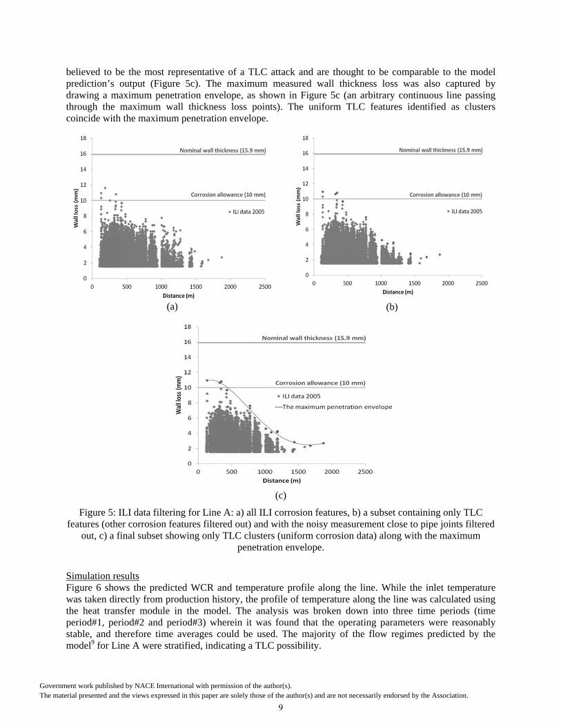
believed to be the most representative of a TLC attack and are thought to be comparable to the model prediction’s output (Figure 5c). The maximum measured wall thickness loss was also captured by drawing a maximum penetration envelope, as shown in Figure 5c (an arbitrary continuous line passing through the maximum wall thickness loss points). The uniform TLC features identified as clusters coincide with the maximum penetration envelope.

(a) (b)

(c)

Figure 5: ILI data filtering for Line A: a) all ILI corrosion features, b) a subset containing only TLC features (other corrosion features filtered out) and with the noisy measurement close to pipe joints filtered

out, c) a final subset showing only TLC clusters (uniform corrosion data) along with the maximum penetration envelope.

Simulation results Figure 6 shows the predicted WCR and temperature profile along the line. While the inlet temperature was taken directly from production history, the profile of temperature along the line was calculated using the heat transfer module in the model. The analysis was broken down into three time periods (time period#1, period#2 and period#3) wherein it was found that the operating parameters were reasonably stable, and therefore time averages could be used. The majority of the flow regimes predicted by the model9 for Line A were stratified, indicating a TLC possibility.

9


For the 1st time period, high values of WCR were calculated at the beginning of the pipeline, due to the higher temperature gradient between the inside and outside of the pipe wall. The predicted WCR values are naturally lower when the pipeline is buried and decrease along the pipeline because of the reduction of internal fluid temperature. For the 2nd time period, the values of WCR were higher than for the 1st time period at the same locations; however, on many other locations the increase in gas velocity led to a change in flow regime prediction to non-stratified, thus eliminating the risk from TLC. This change is flow regime only affected some sections of the entire line but not the entire line. For the 3rd time period, the predicted WCR is clearly lower than for the first two time periods, mostly because of the lower fluid temperature and lower heat exchange between the pipeline fluids and the environment. In summary, the inlet temperature appeared to be the main parameter affecting to WCR in this case. It is consequently crucial to obtain accurate inlet temperature data in order to maximize the accuracy of the predictions.

(a) (b)

(c)

Figure 6: WCR and temperature profile along the length of the pipeline predicted from heat and mass transfer line model simulation: a) First time period, b) Second time period, c) Third time period.

10


Figure 7 shows the predicted TLC rate. High severity of TLC was predicted for the 2nd time period on sections of pipe experiencing stratified flow. This is due to the fact that this time period experienced the most severe combination of high inlet temperature and high inlet pressure. These parameters all contribute to making the environment very corrosive. Cumulative wall thickness loss data are presented in Figure 8 and indicate a high overall risk for TLC in this pipeline. These cumulative values are back-calculated from the predicted corrosion rates obtained for each period and the durations of each period.

Figure 7: Predicted TLC rate for Line A.

Figure 8: Calculated wall thickness loss values for the three time periods and the total cumulative wall thickness loss value.

Comparison between the model prediction and field data In Figure 9, the analyzed ILI data (including error bars equivalent to ±10% wall thickness stemming from instrument accuracy), are compared with the cumulative wall thickness loss predicted by the TLC model. Overall, the predicted TLC line is in good agreement with the maximum wall thickness loss ILI data (i.e. the maximum penetration envelope). It is worth stressing that these model predictions do not consider chemical inhibition while the line itself was batch treated on a monthly basis. The reasonable agreement of the predictions and the ILI measurements is most likely an indication of a fairly ineffective TLC

11


mitigation method, since the model has been successfully validated for a number of other uninhibited environments.9 Over-prediction is noted at the beginning of the line (first 200 meters), but the remainder of the predicted results follows the trend outlined by the maximum penetration envelope and is within the margin of error of the ILI measurements. The discrepancy encountered at the beginning of the line is a recurrent feature of comparison between the model and field data. Our current understanding of the mechanisms tells us that TLC should be more severe when the fluid temperature and the condensation rate are higher. This is the case at the beginning of the line. The reason why the TLC rate does not exactly follow that trend in the first few hundred meters of line is not entirely clear. This discrepancy represents a gap in the understanding of the TLC mechanisms and influential factors as it appears quite consistently, and the model is only a faithful reflection of the current understanding. Although no definitive answer can be given at this stage, the effect of co-condensation of hydrocarbons, which should be quite important at the beginning of the line, could influence the TLC rates. This is despite recent experimental data that seem to suggest otherwise18. Partial transport of inhibitor through droplets that are atomized in the highly turbulent section of pipe following the dogleg could play a role as well.

Figure 9: Comparison between filtered MFL data (with error bars equivalent to ±10% wall thickness due to instrument accuracy) and the TLC model predictions.

Part II: Analysis of other lines In order to determine the validity of the newly-developed methodology and the accuracy of the TLC model, a similar analysis was done for another seven lines for which complete data sets were available. A summary of that work is presented in Figure 10 for another four lines. In all cases, the maximum penetration envelope for the ILI data agrees well with the clustered data (representing uniform TLC) suggesting that the mode of corrosion was not the typical pitting mode but was rather representative of a situation where fairly large local spots on the metal surface are suffering from uniform corrosion. The performance of the TLC model can be considered reasonable for Lines B, D and E, as the predictions agree well with the maximum penetration envelope, with the exception of the first few hundred meters of line where TLC rates are over-predicted. This discrepancy relates to the same gap in the understanding highlighted in the previous section, which is important, as the first sections of the line are commonly a major concern in terms of TLC. For Line C, the model slightly under-predicts the rate of TLC attack along the entire line. However, when error bars are taken into account, this difference does not seem to be statistically significant. This is summarized in Figure 11 where a parity plot is shown for all eight lines that were analyzed. Only the maximum wall thickness loss ILI data for an entire line was used here, and

12


this was compared with the prediction for the same location in the line. A reasonable agreement is obtained in six of the eight cases, which is within the margins of measurement error. In the other two cases the error was more than ±10%.

Figure 10: Comparison between TLC model prediction and reprehensive corrosion features filtered from MFL data. (a) Line B (b) Line C (c) Line D (d) Line E.

Line B Line C

Line D Line E

13


Figure 11: Parity plot between maximum wall thickness loss obtained from the ILI data and the predicted TLC data for eight different lines.

DISCUSSION

The purpose of this paper was in part to validate a mechanistic TLC model, but even more so to propose a procedure that takes into account the intricacy of field data for an effective comparison with model predictions. In this sense, the steps proposed for performing a thorough analysis of the operating conditions and ILI results constitute a clear improvement compared to what has been done in the past16.

It is crucial to ensure that the input parameters “fed” to any model are, as much as possible, an accurate representation of the changing conditions (temperature, pressure, flow rate) encountered in the field.

ILI data should also be thoroughly analyzed in order to extract relevant data that the model was designed to predict.

Overall, in this exercise, the mechanistic TLC model predictions show a reasonably good agreement with the ILI data. However, the comparisons are obviously not “spot-on”, nor should they be expected to be. The procedure cannot fully account for all the inherent complexities of field measurement or account for any lack of understanding in the modeling approach. Since the TLC prediction model used in this study is mechanistic, it is only a reflection of the current knowledge and cannot be expected to predict phenomena which are not yet understood. A clear gap between model prediction and ILI results exists in the first few hundred meters of line. The model predicts the highest TLC rates at the inlet of the line (due to high temperature and water condensation rates), while the ILI data consistently show a maximum in TLC rates a few hundred meters from the inlet. The reason for this specific behavior of the TLC rate at the inlet of the pipe is unknown and should be subject to further investigation in order to verify whether this represents a TLC-specific mechanism or something else (co-condensation, inhibited droplet deposition, protectiveness of corrosion product layer, etc.). In any case, results of model simulation when carefully used in conjunction with field experience significantly improve our ability to understand the main causes of corrosion and implement suitable methods to mitigate them in the future. In the case of the mechanistic TLC model used in the study, the results show that it can be used to evaluate the risk levels for TLC in various pipelines and to prioritize TLC mitigation programs and pipeline corrosion inspection strategies.

SUMMARY

An effective methodology was developed to analyze and validate the field data prior to any comparison with model predication. This included the processing of key operating parameters (inlet temperature, pressure, flow rate), which are known to vary over time, as well as line topography and ILI data, which are inherently complicated and not always reliable. These steps are seen to be crucial for enabling an effective comparison with model predictions.

The mechanistic TLC prediction model used in this study showed a reasonable agreement with the ILI data for most of the lines analyzed, and predicted results within the margins of ILI measurement error. Faults in model performance caused by our lack of understanding were nevertheless identified, especially pertaining to the first few hundred meters of line where the gap between predictions and ILI data was the greatest.

ACKNOWLEDGEMENTS

The authors would like to acknowledge the technical guidance and financial support provided by the sponsoring companies of the Top of the Line Corrosion Joint Industry Project at Ohio University: BP, ConocoPhillips, Chevron, ENI, Occidental Oil Company, PTTEP, Saudi Aramco and Total.

14


REFERENCES

1. Y. Gunaltun, D. Supriyataman and A. Jumakludin, “Top of the line corrosion in multiphase gas line. A case history”, CORROSION/99, paper no. 36 (Houston, TX, 1999). 2. Y. Gunaltun and D. Larrey, “Correlation of cases of top of the line corrosion with calculated water condensation rates”, CORROSION/900, paper no. 71 (Houston, TX, 2000). 3. M. Thammachart, Y. Gunaltun and S. Punpruk, “The use of inspection results for the evaluation of batch treatment efficiency and the remaining life of the pipelines subjected to top of line corrosion”, CORROSION/08, paper no. 8471 (Houston, TX, 2008). 4. Y. Gunaltun, S. Punpruk, M. Thammachart, T. Pornthep, “Worst-case TLC: Cold spot corrosion”, CORROSION/10, paper no. 10097 (Houston, TX, 2010). 5. M. Joosten, D. Owens, A. Hobbins, H. Sun, M. Achour, D. Lanktree, “Top-of-line corrosion – A field failure”, EUROCORR/10, paper no. 9524 (Moscow, Russia, 2010). 6. C. de Waard, U. Lotz, D.E. Milliams, “Predictive model for CO2 corrosion engineering in wet natural gas pipelines”, Corrosion 47, 12 (1991): pp. 976-985. 7. F. Vitse, S. Nesic, Y. Gunaltun, D. Larrey de Torreben, P. Duchet-Suchaux, “Mechanistic model for the prediction of Top-of-the-Line corrosion risk”, Corrosion 59, 12 (2003): pp. 1075-1084. 8. R. Nyborg and A. Dugstad, “Top of the line corrosion and water condensation rates in wet gas pipelines”, CORROSION, paper no. 7555 (Nashville, TN, 2007). 9. Z. Zhang, D. Hinkson, M. Singer, H. Wang, S. Nesic, “A mechanistic model of Top-of-the-Line corrosion”, Corrosion 63, 11 (2007): pp. 1051-1062. 10. S.L. Asher, W. Sun, R.A. Ojifinni, S. Ling, C. Li, J.L. Pacheco and J.L. Nelson, “Top of the line corrosion modeling in wet gas pipelines”, 18th INTERNATIONAL CORROSION CONGRESS, Paper no. 303 (Perth, Australia, 2011) 11. D. Hinkson, Z. Zhang, M. Singer, S. Nesic, “Chemical composition and corrosiveness of the condensate in Top-of-the-Line corrosion”, Corrosion 66, 4 (2010): pp. 045002-045002-8. 12. M. Singer, A. Camacho, B. Brown, S. Nesic, “Sour Top-of-the-Line Corrosion in the presence of acetic acid”, Corrosion 67, 8 (2011): pp. 085003-1-085003-16. 13. J. Amri, E. Gulbrandsen, R.P, Nogueira, “Propagation and arrest of localized attacks in carbon dioxide corrosion of carbon steel in the presence of acetic acid”, Corrosion 66, 3 (2010): pp. 035001-035001-7. 14. Y. Sun, T. Hong, C. Bosch, “Carbon dioxide corrosion in wet gas annular flow at elevated temperature”, Corrosion 59, 8 (2003): pp. 733-740. 15. M. Singer, “Study and Modeling of the Localized Nature of Top of the Line Corrosion”, PhD Dissertation, Ohio University, 2013. 16. Y. Gunaltun, U. Kaewpradap, M. Singer, S. Nesic, S. Punpruk and M. Thammachart, “Progress in the prediction of top of the line corrosion and challenges to predict corrosion rates measured in gas pipelines,” CORROSION/10, paper no. 10093 (San Antonio, TX, 2010). 17. U. Kaewpradap, M. Singer, S. Nesic, S. Punpruk, “Top of the line corrosion – Comparison of model predictions with field data”, CORROSION/12, paper no. 1449 (Salt Lake City, UT, 2012). 18. T. Pojtanabuntoeng, M. Singer, S. Nesic, “Water/Hydrocarbon co-condensation and the influence on top-of-the-line corrosion”, CORROSION/11, paper no. 11330 (Houston TX, 2011). 19. M. Singer, D. Hinkson, Z. Zhang, H. Wang, and S. Nesic, "CO2 Top-of-the-Line Corrosion in Presence of Acetic Acid: A Parametric Study", Corrosion 69, 7 (2013): pp. 719. 20. R. Hall, M. McMahon, “Report on the use of in-line inspection tools for the assessment of pipeline integrity”, US Department of Transportation, Report No. DTRS56-96-C-0002-008, 2002. 21. Pipeline Operators Forum (POF) document, “Specifications and requirements for intelligent pig inspection of pipelines”, 2009.

15


Paper No. 5809 - Ohio University

Documents

Transcript of Paper No. 5809 - Ohio University